Recurrent Neural Network-based Anti-jamming Framework for Defense Against Multiple Jamming Policies

Abstract

Conventional anti-jamming methods mainly focus on preventing single jammer attacks with an invariant jamming policy or jamming attacks from multiple jammers with similar jamming policies. These anti-jamming methods are ineffective against single jammer following several different jamming policies or multiple jammers with distinct policies. Therefore, this paper proposes an anti-jamming method that can adapt its policy to current jamming attack. Moreover, for the multiple jammers scenario, an anti-jamming method that estimates the future occupied channels using the jammers’ occupied channels in previous time slots is proposed. In both single and multiple jammers scenarios, the interaction between the users and jammers is modeled using recurrent neural networks (RNN)s. The performance of the proposed anti-jamming methods is evaluated by calculating the users’ successful transmission rate (STR) and ergodic rate (ER), and compared to a baseline based on Q-learning (DQL). Simulation results show that for the single jammer scenario, all the considered jamming policies are perfectly detected and high STR and ER are maintained. Moreover, when $70\%$ of the spectrum is under jamming attacks from multiple jammers, the proposed method achieves a STR and ER greater than $75\%$ and $80\%$, respectively. These values rise to $90\%$ when $30\%$ of the spectrum is under jamming attacks. In addition, the proposed anti-jamming methods significantly outperform the DQL method for all the considered cases and jamming scenarios.

I Introduction

Wireless communication networks are susceptible to jamming attacks due to their shared and open nature. Jamming attacks cause performance degradation or denial of service by disrupting communication links in wireless networks. Therefore, it is necessary to adopt anti-jamming methods to mitigate such attacks. Various anti-jamming techniques have been proposed in the literature; however, the majority of available techniques is focused on preventing a single type of jamming attack. For instance, the authors in [2, 3, 4, 5] mainly focus on mitigating reactive jammer attacks while [6] and [7] perform anti-jamming against sweeping jammers. Some machine learning-based anti-jamming techniques that can work against several jammer types, such as [8], assume that during interactions between legitimate users and jammers, the policies of the jammers remain unchanged. Thus, if the policy of a jammer changes, legitimate nodes must be retrained, resulting in a performance loss. Therefore, there is a pressing need for an anti-jamming method capable of mitigating multi-type jammer attacks.

When confronted with a single jammer that can adopt different jamming policies, it is necessary to first recognize the jammer’s policy, and then select an appropriate countermeasure. Jamming recognition techniques are mainly studied in the context of radar [9, 10, 11, 12], with a focus on detecting the jammer’s type utilizing the jamming signals. In [9], the power spectrum of the jamming signal is used to determine the type the jammer. In [10], the authors utilize the fast Fourier transform (FFT) of the jamming signal to recognize the jamming policy while in [11] and [12] the time domain signal is used. The authors in [13] employ convolutional neural networks (CNNs) to recognize the jamming type using a waterfall plot of the spectrum.

From a practical perspective, implementing the recognition techniques from [10, 11, 12, 9] requires accurate samples from the jamming signal. Moreover, the recognition technique in [13] is limited to simple jamming policies and requires a large data set for training. Thus, it is necessary to develop an anti-jamming technique that can work with a small data set for training and can be extended to different types of jamming.

In addition, the presence of multiple jammers with different jamming policies gives rise to additional challenges in wireless networks. However, most previous works, such as [2, 3, 4, 5, 6, 7], consider the single jammer case. Some works, such as [14, 15, 16, 17] consider multiple jammers with similar jamming policies. Specifically, the authors in [14] and [15] formulate the interaction between a user and several jammers as a non-cooperative game where the utility functions of the jammers are the same. In [14] the latency is considered as the utility function of the jammers while in [15] the SINR is set as the jammers’ utility function. The authors in [16] propose to harvest the reactive jammers’ energy and use backscatter to relay the user’s data. Similarly, the work in [17] considers a multi-function wireless system and employs a backscatter as a redundant communication path when the main path is under threat from reactive jammers. Moreover, the works in [18, 19, 20] focus on the localization of the multiple jammers and do not propose any anti-jamming methods. In the context of Unmanned aerial vehicles (UAVs), the works in [21, 22, 23] attempt to determine the trajectory for UAVs that are under attack by multiple jammers to avoid jamming attacks. In [24] and [25], the authors propose a channel allocation method based on spectrum sensing. In this context, the users share their local spectrum sensing with each other to select the channels that are less probable to be jammed.

Although the works in [16, 14, 15, 17, 18, 19, 20, 21, 22, 23, 25, 24] study scenarios with multiple jammers, they suffer from several drawbacks, which make them impractical against multiple jammers with different jamming policies. The assumption of similar policies at the jammers is a major drawback in all the above mentioned works. Moreover, some of these works such as [14] and [15], assume the availability of the channel gains between the user and jammers, which is not practical. The considered schemes in [16] and [17] are restricted to specific system models because a backscatter is employed to relay the users’ data in case of jamming attacks. The proposed solutions in [21, 22, 23] can only be applied to UAVs, and therefore is unsuited for a wider range of applications. The authors in [24] and [25] propose to monitor the jammers’ occupied channels in previous time slots to allocate free channels to the users in future time slots. This approach is practical against multiple jammers with multiple jamming policies since they focus on determining free channels in future time slots instead of selecting a countermeasure for a specific type of jamming attack. However, the exploitation of the obtained knowledge is inefficient since these methods only utilize the information of the spectrum in the last time slot while the information of the spectrum occupancy in previous time slots can be utilized to better understand the spectrum occupancy pattern.

In light of the above discussion, it is obvious that the problem of a wireless network under jamming attacks from multiple jammers with multiple jamming policies needs to be investigated. Thus, in the second part of the paper, we propose an anti-jamming technique for multiple jammers with different jamming policies.

The main contribution of this paper is to propose two novel anti-jamming methods against a single jammer capable of launching attacks with different jamming policies and multiple jammers with different jamming policies. In order to defend the single jammer, we develop an anti-jamming method that requires a small data set for training and is practical against several jamming types. In this context, the jammer’s type is first detected, and then an appropriate countermeasure is selected. For multiple jammers with different jamming policies, we propose to estimate the jammers’ future behavior from their occupied channels in previous time slots. In both of the proposed anti-jamming techniques, the occupied channels of the jammers in previous time slots are stored, and based on the obtained information, the jamming policy or jammers’ future occupied channels will be estimated. Due to the sequential nature of the interaction between users and jammers, we propose the use of recurrent neural networks (RNNs) in both cases. To evaluate our methods, we calculate the ergodic rate (ER) and perform different simulations considering different jamming policies. Our results show that in the single jammer scenario, the jamming policies are detected perfectly with high accuracy within a short period, and as a result, the best countermeasure is employed, leading to a high successful transmission rate (STR) and ER for the user. Moreover, against multiple jammers, the proposed anti-jamming technique achieves a STR and ER higher than $75\%$ when $70\%$ of the spectrum is being jammed. This value rises to $90\%$ when $30\%$ of the spectrum is being jammed.

The rest of this paper is organized as follows. Section II presents the system model and problem formulation. In sections IV and V, we present the proposed anti-jamming methods for single and multiple jammer scenarios, respectively. Simulation results are shown in Section VI and conclusions are drawn in Section VII.

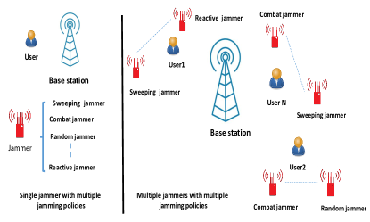
Figure 1: Considered system model.

II System Model and Problem Formulation

II-A System model

We consider a wireless network composed of a BS, $N$ users, and $J$ jammers. We study two distinct scenarios based on the number of jammers in the network. In the first scenario (SC1), the network includes a user and a jammer capable of attacking with various jamming policies, while in the second scenario (SC2), we assume that multiple users are attacked by multiple jammers with different jamming policies. In both scenarios, the BS is located at the center of the network while users and jammers are randomly distributed in the network, as shown in Fig. 1. In both scenarios, we assume that the network is constantly under jamming attacks. In SC2, each user is assumed to be located within the communication range of at least one jammer. Time is divided into time slots, where at each time-slot, each user is served using a channel selected from $L$ channels. The packet transmitted by a user over a frequency channel is successfully received when that channel is not jammed or interfered by other users. Four types of jamming policies are considered, where in each time slot, each jammer can jam several frequency channels. The considered jamming policies are:

• Random jammer, which chooses its channels randomly.

• Sweeping jammer, which periodically shifts its full energy over multiple frequency channels.

• Reactive jammer, which listens to channels repeatedly and jams channels after a single time slot from sensing an activity.

• Combat jammer, which chooses a number of channels randomly and jams them for a number of consecutive time slots.

In SC1, the jammer selects a policy from the above-mentioned policies while in SC2, we assume that each user is attacked by a group of jammers employing all of the above-mentioned jamming policies. In both scenarios, we assume that each user can sense the jamming signals in the frequency channels to detect occupancy. In this context, if the sensed amplitude of the base-band signal of a channel is higher than a specific threshold, the channel is counted as an occupied channel, otherwise, it is assumed to be free.

II-B Problem formulation

We now formally formulate the interaction between users and the jammers as an optimization problem. To this end, assuming that the vector of the indices of all frequency channels allocated to users under policy $\pi$ is given by

$$\boldsymbol{c}^{\pi}=[c^{\pi}_{1},c^{\pi}_{2},...,c^{\pi}_{N}],$$ (1)

where $c^{\pi}_{N}$ denotes the index of the $i^{th}$ user’s selected channel under policy $\pi$, the instantaneous sum rate of the network at time slot $t$ is defined as

$$R=\sum_{k=1}^{N}\mathbb{I}(c^{\pi}_{k})\log_{2}\left(1+\frac{\Omega_{k}|h_{kc_{k}}|^{2}}{\delta^{2}}\right),$$ (2)

where $t$ denotes the time slot index, $h_{kc_{k}}$ is the channel gain between the $k^{th}$ user and the BS in frequency channel $c_{k}$, $\Omega_{k}$ is the $k^{th}$ user’s power, $\delta^{2}$ is the noise power, and $\mathbb{I}(\cdot)$ is an indicator function given by

$$\mathbb{I}(c^{\pi}_{k})=\left\{\begin{array}[]{ll}0,&\mbox{if }c^{\pi}_{k}\mbox{ is jamming and collision free.}\\ 1,&\mbox{otherwise,}\end{array}\right.$$ (3)

Our goal is to obtain a channel allocation strategy $\pi$ that allocates free frequency channels to the users at each time slot. Hence, we set the instantaneous sum rate of the network as the objective function of the optimization problem. As a result, the design of the optimal strategy $\pi^{*}$ for the users’ channel allocation can be formulated as the following optimization problem:

$$\underset{\pi}{\textnormal{maximize}}{\hskip 14.22636ptR},$$ (4)

$$\textnormal{s.t.}\hskip 14.22636pt\textnormal{ }|\mathbb{A}|\geq{J}\textnormal{ and }|\boldsymbol{c}^{\pi}|=N\hskip 2.84544pt\forall t,$$

where $\mathbb{A}=\{\boldsymbol{u}_{1},\boldsymbol{u}_{2},...,\boldsymbol{u}_{J}\}$ denotes the selected frequency channels by the jammers and $\boldsymbol{u}_{i}$ is a vector containing the indices vector of the $i^{th}$ jammer’s selected frequencies. The constraints $|\mathbb{A}|\geq{J}$ and $|\boldsymbol{c}^{\pi}|=N$ imply that each jammer jams at least one channel and one frequency channel is assigned to each user at each time slot, respectively.

In each iteration of the interaction between the users and the jammers, the users must find the optimal channels. Problem (LABEL:opt) is a discrete optimization problem aiming to maximize the users rate by selecting the optimal channel between the users and the BS. In this context, the optimal choice for each user is to select the channel that has the highest channel gain between the user and the BS among free channels. In order to characterize the maximum achievable ER, we consider an ideal case each user knows the jammed channels in the next time slot. We use a Nakagami $m$-fading distribution with average channel power gain $\lambda$ to model the channel gain between each user and the BS. The total number of jammed channels around the $k^{th}$ user is $\boldsymbol{\upsilon}_{k}$, the ER of the $k^{th}$ user is obtained using Proposition 1.

Figure 2: GRU network.

Proposition 1.

The ER of the $k^{th}$ user when the highest channel gain between this user and the BS is selected will be:

$$R_{ek}=\frac{\Omega_{k}}{\delta^{2}\ln{(2)}}\int_{0}^{\infty}\frac{1-(\frac{\gamma(m,\frac{mx}{\lambda})}{\Gamma(m)})^{(L-\upsilon_{k})}}{1+\frac{\Omega_{k}x}{\delta^{2}}}dx$$ (5)

Proof.

See Appendix A. ∎

When the users interfere with each other, the ER of each user can be obtained by slightly modifying (LABEL:erg1). In this context, the number of free channels for each user reduces to $L-N-\upsilon_{k}+1$. Thus, the ER of the $k^{th}$ user will be:

$$R_{e\zeta_{1}}=\frac{\Omega_{k}}{\delta^{2}\ln{(2)}}\int_{0}^{\infty}\frac{1-(\frac{\gamma(m,\frac{mx}{\lambda})}{\Gamma(m)})^{(L-N-1-\upsilon_{k})}}{1+\frac{\Omega_{k}x}{\delta^{2}}}dx.$$ (6)

In some cases, it is recommended to select the users’ channels by following a random policy that can minimize the probability of being traced by the jammers. In this context, the ER of the $k^{th}$ user will be obtained using Proposition 2.

Proposition 2.

The ER of the $k^{th}$ user when the user selects its channels randomly is given as

$$R^{\prime}_{ek}=\frac{1}{\Gamma({m})\ln({2})}G_{2,3}^{3,1}\left(\frac{\delta^{2}m}{\Omega_{k}\lambda}\bigg{|}\begin{matrix}0,1\\ 0,0,m\end{matrix}\right)$$ (7)

Proof.

See Appendix B. ∎

The equation in (7) is valid for both the ideal and interference scenarios. For all the aforementioned scenarios, the ergodic sum rate can be obtained by taking the sum of all the users’ rates. We note that the obtained ER using (LABEL:erg1) and (7) are the maximum achievable ERs since they are calculated assuming that each user knows the other users’ and jammers’ occupied channels in future time slots.

In order to solve (LABEL:opt), the jammers’ selected channels at the next time slot, i.e, $\mathbb{A}$, must be known; however, in realistic scenarios, this information is not available. Therefore, next, we propose RNN-based anti-jamming methods to predict the occupied channels by the jammers in the next time slot.

III Proposed anti-jamming method against single-jammer

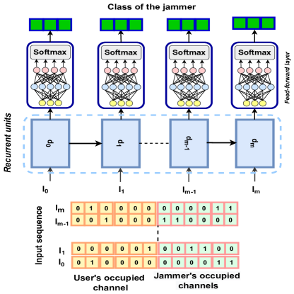
Figure 3: Proposed RNN for single jammer scenarios.

We now introduce the proposed anti-jamming method in SC1. Since the user is attacked by a jammer that can jam with different jamming policies, we propose to first recognize the jamming policy, and then select an appropriate countermeasure against the jammer. In this context, the interaction between the user and the jammer is sequential. We thus employ RNNs because of their ability to process data with a sequential nature. RNNs are artificial neural networks that can learn patterns and long-term relationships from time series and sequential data. At each time slot, an RNN takes the previous hidden state and the input, and generates the updated hidden state and output as follows [26]

(8)

$$\boldsymbol{d}_{t}=\sigma(\boldsymbol{K}_{d}\boldsymbol{d}_{t-1}+\boldsymbol{V}_{\boldsymbol{d}}\boldsymbol{l}_{t}+\boldsymbol{g}_{\boldsymbol{d}})$$

$$\boldsymbol{y}_{t}=\sigma(\boldsymbol{K}_{y}\boldsymbol{d}_{t}+\boldsymbol{g}_{\boldsymbol{y}}),$$

where $\boldsymbol{l}$ is the input, $\boldsymbol{d}_{t}$ is the hidden state at time slot $t$, $\sigma$ is an activation function, $\boldsymbol{V}_{\boldsymbol{d}}$ is the weight of the input vector, $\boldsymbol{g}_{\boldsymbol{d}}$ and $\boldsymbol{g}_{y}$ are the bias terms, and $\boldsymbol{K}_{\boldsymbol{d}}$ and $\boldsymbol{K}_{y}$ denote the weights of the hidden layer and the output, respectively. High depth and recurrent connections in conventional RNNs cause a vanishing gradients problem. This vanishing gradient challenge is addressed in gated recurrent unit (GRU)[27] models by controlling the inputs using multiple gates in a hidden layer.

In this context, based on the conditions of the input and previous hidden layer, the controller gate $r_{t}$ is set to one or zero to update the hidden layer. The overall process is shown in Fig. 2. At time slot $t$, the GRU states are updated as follows:

(9)

$$\boldsymbol{r}_{t}=S(\boldsymbol{W}_{r}\boldsymbol{l}_{t}+\boldsymbol{U}_{z}\boldsymbol{d}_{t-1}+\boldsymbol{g}_{r})$$

$$\boldsymbol{z}_{t}=S(\boldsymbol{W}_{z}\boldsymbol{l}_{t}+\boldsymbol{U}_{z}\boldsymbol{d}_{t-1}+\boldsymbol{g}_{z})$$

$$\hat{\boldsymbol{d}_{t}}=\tanh(\boldsymbol{W}_{{\boldsymbol{d}}}.\boldsymbol{l}_{t}+\boldsymbol{U}_{\boldsymbol{d}}.(\boldsymbol{z}_{t}\odot\boldsymbol{d}_{t-1})+\boldsymbol{g}_{{\boldsymbol{d}}})$$

$$\boldsymbol{d}_{t}=(1-\boldsymbol{r}_{t})\odot\boldsymbol{d}_{t-1}+\boldsymbol{r}_{t}\odot\hat{\boldsymbol{d}_{t}},$$

where $\boldsymbol{W}_{\boldsymbol{r}}$, $\boldsymbol{U}_{\boldsymbol{r}}$, $\boldsymbol{W}_{l\boldsymbol{z}}$, $\boldsymbol{W}_{\boldsymbol{z}}$, $\boldsymbol{W}_{\boldsymbol{d}}$, $\boldsymbol{U}_{\boldsymbol{d}}$, $\boldsymbol{g}_{\boldsymbol{r}}$, $\boldsymbol{g}_{\boldsymbol{z}}$, and $\boldsymbol{g}_{\boldsymbol{d}}$ are learning parameter matrices and vectors. Here the operator $\odot$ represents the Hadamard product, and $S$ is the Sigmoid function.

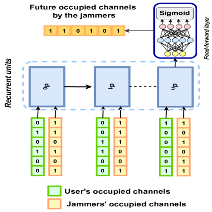
Figure 4: Proposed RNN for multiple jammers scenarios.

A feed-forward layer with an output size equal to the number of considered jamming classes is considered after each GRU hidden state. Then, the output of the feed-forward layer is passed through a SoftMax layer to generate a probability distribution vector for the jamming type classes. It is noted that the predicted class is obtained by the index of the output array that has the highest probability value. In Fig. 3, we show the proposed network.

We divide the proposed recognition technique into training and testing. In the training phase, which is an offline process, the interaction between the user and the jammer is simulated. In contrast, the testing is an online process that takes place during the interaction between the user and the jammer.

The interaction between the user and the jammer is simulated for $T$ consecutive time slots. During the simulation, a channel is randomly assigned to the user and the jammer’s responses for all of the considered jamming policies, i.e, random, sweeping, reactive, and combat, are simulated and the channels of the users, the jammer, and corresponding jamming policies are saved. At each time slot, a vector with $2L+1$ elements is considered. The first and second $L$ elements are used to save the user’s and jammer’s utilized channels, respectively. Specifically, the $i^{th}$ element of the vector is set to one if the $i^{th}$ channel is occupied by the user, otherwise it is set to zero. The same procedure is used to denote the jammer’s occupied channels. Finally, the jamming policy class is stored in the $(2L+1)^{th}$ element. Given that the number of channels jammed in each time slot, in addition to the jammers’ channel selection policies, is crucial, a distinct class is assigned to each combination of jamming policy and number of jammed channels. For instance, a sweeping jammer that jams two channels per time slot is not in the same class as one that jams one channel. As a result, a sweeping jammer with one to four channels must have four classes assigned to it.

The collected data from the simulations is then used to train the proposed RNN. Here, the elements with column indices from $1$ to $2L$ are the inputs while elements in the $2L+1^{th}$ column are the corresponding class targets. During every step of the training, a matrix consisting of $a$ consecutive vectors is fed to the RNN and a vector with the same number of elements as the number of classes is generated by the network. We employ the cross-entropy as the loss function to train the network.

In the testing phase, similar to the training process, the user’s and jammer’s occupied channels in the last $b$ time slots are saved. In this context, the selected channels by the user and jammer during the last $b$ time-slots are given to the trained network, and the network then generates a vector. The class of the jammer is determined by the index of the highest value in the output vector. Anti-jamming can be easily selected once the jamming policy and corresponding number of jammed channels are identified. In this context, the future behavior of the combat, sweeping, and reactive jammers can be predicted from the detected class of the jammer and the jammer’s selected channels in previous time slots. Thus, the user can find the best channel that maximizes its rate among free channels. For instance, if the trained network detects that the channels are jammed by a sweeping jammer in which jams three channels per time slot, users predict that the sweeping jammer will jam channels with indices $5$ to $7$ in the coming time slot when the indices of jammed channels in previous time slot are $2$ to $4$. Thus, users will select channels other than channels with indices $5$ to $7$. For the random jammers, the future channels that the jammer will select cannot be determined. In this case, the user selects a channel randomly among all channels.

IV Proposed anti-jamming method against multiple jammers

In SC2, users are simultaneously attacked by multiple jammers with different jamming policies. In this context, users cannot differentiate between the jamming policies of each jammed channel, and thus the proposed anti-jamming method in SC1 cannot be employed. We propose to estimate the channels that will be jammed in the next time slot using the jammers’ occupied channels in previous time slots. Once more, the interaction between the users and the jammers has a sequential nature, and therefore we also use RNNs in SC2. We consider two scenarios depending on whether or not users interfere with each other. Since we assume that the status of a frequency channel is solely determined by sensing the signal amplitude of that channel and no signal processing is performed, the users cannot distinguish between a jammed and an interfered channel.

In SC2, we consider an RNN for each user. In this context, after each GRU hidden layer, we use a feed-forward layer with output size equal to the number of channels, as depicted in Fig. 4. Next, the output of the fully connected layer is fed into a Sigmoid function to normalize the output elements between zero and one. Afterwards, the values that are higher than $0.5$ are set to one and the ones lower than $0.5$ to zero.

Similarly, the proposed anti-jamming method is divided into two phases, i.e. training and testing. In each time slot of the training phase, each user considers a vector with $2L$ elements, and saves its utilized channel in the first $L$ elements while the occupied channels by jammers are saved in the second $L$ elements (and other users in case of interference). Particularly, the $i^{th}$ element is set to one if the $i^{th}$ channel is occupied, otherwise it is set to zero. During training, we use a random channel selection policy for the users so as to generalize the results. However, the proposed training scheme can work with any other channel allocation methods. To provide the target data, the vector containing the occupied channels in the current time slot is used as the target of the previous time slots because we want to estimate the occupied channels in the next time slot.

During every step of the training, a matrix consisting of $a$ consecutive vectors is fed to the RNN, and a vector with $L$ elements is generated by the network. The binary cross-entropy is utilized as the loss function to train the network. The testing process of SC2 is similar to that in SC1 with a slight change that estimated occupied channels in the next time slot is outputted from the trained network.

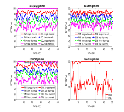
Figure 5: STR of the proposed anti-jamming method.

In the two anti-jamming techniques proposed in this work, the information about the jammed channels is required. To extract this information, each user senses all the frequency channels and flags channels where the amplitude of the base-band signal is higher than a specific threshold. In this context, the received jamming signal in a frequency channel is given as:

$$\chi_{k}=\Upsilon_{k}+n,$$ (10)

where $\Upsilon_{k}$ is the amplitude of the jamming signal at the $k^{th}$ user’s side and $n$ is the white Gaussian noise with power $\delta^{2}$. Assuming that the detection threshold is $\Gamma$, a miss-detection happens when the noise amplitude is lower than $n\leq(\Gamma-\Upsilon_{k})$ and a false alarm happens when $n\geq\Gamma$. Thus, the probability of miss-detection $P_{\textnormal{md}}$ and false alarm $P_{\textnormal{fa}}$ are given as

$$P_{\textnormal{md}}=Q\left(\frac{\Upsilon_{k}-\Gamma}{\delta}\right),$$ (11)

$$P_{\textnormal{fa}}=Q\left(\frac{\Gamma}{\delta}\right),$$ (12)

respectively. $P_{\textnormal{fa}}$ shows that the probability of false alarm only depends on the value of the threshold and noise power while $P_{\textnormal{md}}$ depends on the jamming signal power at the users’ side.

$\Gamma$ must be high enough to minimize $P_{\textnormal{fa}}$, and should not be too high since increasing $\Gamma$ increases $P_{\textnormal{md}}$. The value of $\Gamma$ can be selected based on the desired values for $P_{\textnormal{md}}$ and $P_{\textnormal{fa}}$, and the jamming- to-noise-ratio (JNR). For instance, $\Gamma$ should satisfy $\frac{\Gamma}{\delta}=2.32$ to have $P_{\textnormal{fa}}=0.01$. Here, $P_{\textnormal{md}}=0.01$ for a JNR of $\frac{||\Upsilon_{k}||^{2}}{\sigma^{2}}=13.35$ dB. For both of the considered scenarios, we set $\frac{\Gamma}{\delta}=2.8117$ and JNR $=15$ dB.

V Simulation Results

We now assess the proposed anti-jamming methods in both considered scenarios using extensive simulations. To this end, we define an evaluation metric, named STR, which quantifies the ratio of the number of successfully delivered packets to all the transmitted packets. For the first scenario, the proposed anti-jamming method is assessed by evaluating the STR and detection accuracy for the different jamming policies as a function of the elapsed time. We consider that random, combat, and sweeping jammers can simultaneously jam one to four channels. Moreover, we compare the output of the proposed anti-jamming method to the case in which the user employs deep Q-learning (DQL) for its anti-jamming and channel allocation policy. In addition, we compare the ER obtained by the proposed anti-jamming techniques to the calculated ER in (LABEL:erg1) and (7). In SC1, simulation results are obtained using $12$ channels. For SC2, we assume that each user is surrounded by a random, a combat, a sweeping, and a reactive jammer. The jammers’ specifications are provided in Table I. The proposed anti-jamming method is evaluated by illustrating the STR of one to four users when $30\%$ to $70\%$ of the spectrum is under jamming attacks. Moreover, results are compared to the case where DQL is employed for the users’ channel allocation. In addition, we show the performance of each jammer in terms of successful jamming attacks to clarify the impact of each jamming type separately. In SC2, simulation results are obtained by considering $20$ channels. Moreover, we choose $a$ and $b$ as $20$, and channels are assumed to follow Rayleigh fading, i.e. $m=1$.

TABLE I: Number of jammed channels by jammers.

	Jamming ratio
Jammer type	30%	40 %	50%	60%	70%
Sweeping jammer	2	3	4	4	5
Reactive jammer	1	1	1	1	1
Random jammer	1	2	2	3	3
Combat jammer	2	2	3	4	5

V-A Anti-jamming in SC1 scenario

In Fig. 5, we show the STR resulting from the proposed anti-jamming method for all the considered types of the jammers. From this figure, we observe that after a few time slots, except for the random case, the obtained STR surpasses $90\%$ and STRs of almost $100\%$ are obtained after $20$ time slots. The STR increases with time since the users are provided with more information from the jammers, which leads to jamming policy detection with a higher accuracy. As a result of a precise jamming policy detection, an appropriate countermeasure against the detected jammer is taken, resulting in a high STR. Lower STR is obtained in the context of random jammers since future channels cannot be estimated even for perfect jamming policy detection. As a result, users have to select their future channels randomly. In this context, increasing the number of jammed channels by the random jammer increases the probability of getting jammed by the jammer. In addition, Fig. 5 shows that the proposed anti-jamming method outperforms the DQL-based anti-jamming method for all the considered cases, except for the Random jammer. Specifically , the proposed method converges within a few time slots while DQL needs more time slots to train the users.

Fig. 6 presents the detection accuracy rate for all the considered jamming policies. From this figure, we observe that, after just five time slots, the sweeping and combat jamming polices are detected perfectly. Detecting the policy of the random and reactive jammers requires more time slots due to the similarity between these jammers’ behavior in initial time slots.

In Fig. 7, we verify the ERs derived is (LABEL:erg1) and (7) using simulations. Here, we consider the number of jammed channels to vary between one to four. The obtained ERs by the proposed anti-jamming method for all the considered jamming scenarios are shown. The The presented graphs in order are: 1) ERs obtained by (LABEL:erg1) with legend of TM, 2) simulation to verify (LABEL:erg1) with legend of SM, 3) proposed anti-jamming method against sweeping and combat jammers with legend of PM-SC, 4) ERs obtained by (7) with legend of TR, 5) simulation to verify (7) with legend of SR, 6) proposed anti-jamming method against random jammer by assigning the channel with the highest channel gain to the user with legend of PM-R-M, and 7) proposed anti-jamming method against random jammer with random channel selection with legend of PM-R-R. Moreover, in Fig. 7, we present the ER resulting from proposed anti-jamming method when the number of jammed channels is one by the legend of PM-RE.

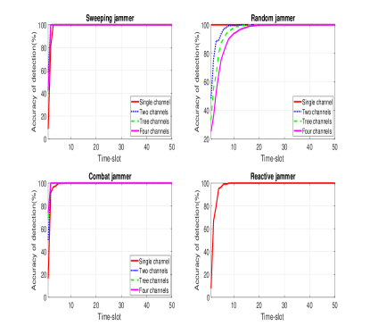
Figure 6: Detection accuracy of the jamming policies as a function of the elapsed time.

The results in Fig. 7 demonstrate that the calculated ERs match perfectly with the simulation results, which proves the accuracy of the derivations. From this figure, we can also see that the ERs in the presence of reactive, sweeping, and combat jammers are close to the maximum achievable ERs. This, in turn, shows the effectiveness of the proposed anti-jamming method in recognizing the jamming policies and assigning high-quality channels to the user. Against the random jammer, the ER is less than the other jammers since the random jammer’s occupied channels in the next time slot are not predictable. Moreover, for all the considered numbers of jammed channels by the random jammer, assigning the channel with the highest channel gain to the user provides a higher ER than the case in which the channel assignment is random.

Figure 7: ER for SC1.

V-B Anti-jamming in SC2 scenario

Fig. 8 presents the users’ STR as a function of the elapsed time slots. From Fig. 8, we can see that the users achieve a STR higher than $90\%$ when $30\%$ of the spectrum is under jamming attacks. This value decreases to $80\%$ when jammers jam $70\%$ of the spectrum. The reason behind this performance degradation is that the users have less free channels to utilize. Moreover, for all the considered scenarios, the proposed method outperforms the DQL-based method with a significant gap.

The STR of the users case of interference is shown in Fig. 9. The performance of the proposed anti-jamming method decreases compared to the interference-free case. This is because the RNN is trained assuming that users choose their channels at random. As a result, each user randomly estimates the future behaviour of other users during the testing process. Moreover, when users interfere with each other, fewer available channels remain for channel selection. For instance, in the four users scenario with $70\%$ of the channels jammed, four users must select their channels out of six available channels while for the case in which the users do not interfere, each user has six available channels.

In Fig. 10, we present each jammer’s success rate individually. These results show that the reactive and sweeping jammers have constant jamming success rates for all the considered jamming ratios. Meanwhile, the random jammer’s success rate increases by increasing the jamming ratio. This is because the reactive jammer has a fixed number of jammed channels for all the considered jamming ratios. Moreover, the future behaviour of sweeping jammer is expectable and as a result, increasing the number of jammed channels in this type of jammer does not impact the success rate. However, it is impossible to predict the channels that the random jammer will choose in the following time slot. Therefore, increasing the number of jammed channels increases the random jammer’s success rate. Similar to random jammers, increasing the number of jammed channels by the combat jammer increases the success rate of the jammer due to randomness in the channel selection of the combat jammer. However, since the combat jammer jams the selected channels for a number of consecutive time slots, the increase in the success rate is lower than that of the random jammers.

Figure 8: STR of the proposed anti-jamming method when users interfere each other.

Fig. 11 compares between the ERs of each user obtained by the proposed method, (LABEL:erg1), and (LABEL:erg2), for both cases with and without interference. Drawn graphs in order are related ERs obtained by: 1) (LABEL:erg1), denoted as TM, 2) (LABEL:erg2) for two users, denoted as TIM-2, 3) (LABEL:erg2) for three users, referred to as TIM-3, 4) (LABEL:erg2) for four users, denoted as TIM-4, 5) proposed method for the case where users do not interfere each other denoted as PM, 6) proposed method for two users scenario while users interfere each other specified with legend PMI-2, 7) proposed method for three users scenario while users interfere each other, denoted as PMI-3, and 8) proposed method for four users scenarios considering users interfere each other, denoted as PMI-4. When users do not interfere with each other, the ER of each user is similar over the different scenarios with different numbers of users. Hence, only the ER of the single-user scenario is plotted. The TM graph shows that the ER is higher when there is no interference. Moreover, when users interfere with each other, increasing the number of users and channels decreases the ER since increasing the number of users and jammed channels decreases the number of available channels for each user. The same trend holds for increasing the number of users and channels in the obtained results by the proposed method, i.e. PM, and PMI-2 to PMI-4. In the case where users do not interfere with each other, results show that the proposed method achieves ERs higher than $80\%$ of the maximum achievable ER for all the considered numbers of jammed channels. Moreover, when $30\%$ of the spectrum is being jammed, the ER is close to $90\%$ of the maximum achievable ER. In the case where users interfere with each other, the discrepancy between the maximum achievable ER and the obtained ER by the proposed method is higher than the case of no interference since fewer free channels are available for the channel selection of each user.

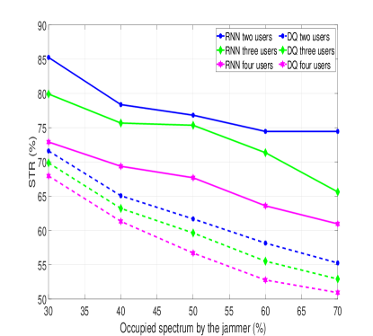
Figure 9: STR of the proposed anti-jamming method when users interfere with each other.

VI Conclusion

In this paper, we proposed RNN-based anti-jamming techniques against single jammer and multiple jammers. Two distinct scenarios based on the number of jammers in the network have been considered. In the first scenario, the network includes a user and a jammer capable of attacking with various jamming policies, while in the second scenario, we have assumed that multiple jammers attack multiple users with different jamming policies. Moreover, we have studied two different cases based on whether users interfere with each other or not. For both of the considered cases, we have calculated the maximum achievable ER. To evaluate the proposed anti-jamming methods, we have performed extensive simulations assuming four jamming policies. Moreover, we have compared the obtained results with the case where DQL is employed. The results show that against a single jammer, all the considered jamming policies are detected with high accuracy within a short period, and as a result of an accurate jamming type detection, high STRs and ERs are obtained. Against multiple jammers, STRs and ERs near $80\%$ are obtained when $70\%$ of the spectrum is under jamming attacks. These values rise to $90\%$ when $30\%$ of the spectrum is under jamming attacks. Moreover, for all the considered numbers of users and jamming ratios, the proposed anti-jamming technique outperforms the DQL algorithm with significant gaps.

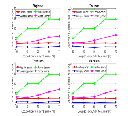
Figure 10: Jammers’ success rate.

Appendix A Proof of Proposition 1

The ER of the $k^{th}$ user is

$$R_{ek}=\mathbb{E}(\mathbb{I}(c^{\pi}_{k})\log_{2}(1+\frac{\Omega_{k}|h_{kc_{k}}|^{2}}{\delta^{2}})).$$ (13)

Assuming that the jammed channels and occupied channels by other users are known, then $k^{th}$ user selects its channels among free channels, and given $x=|h_{kc_{k}}|^{2}$, we can rewrite (13) as follows:

$$R_{ek} =\mathbb{E}(\log_{2}(1+\frac{\Omega_{k}x}{\delta^{2}}))$$ (14)

$$=\frac{1}{\ln{2}}\int_{0}^{\infty}\ln{(1+\frac{\Omega_{k}x}{\delta^{2}})}f_{h_{kc_{k}}}(x)dx,$$

where $f_{h_{kc_{k}}}(x)$ is the probability distribution function (PDF) of $x$. The channel $h_{kc_{k}}$ is selected among $L-\upsilon$ channels, where the power gain of each of the channels is a random variable with PDF

$$f(x)=(\frac{m}{\lambda})^{m}\frac{x^{m-1}}{\Gamma(m)}exp[\frac{-mx}{\lambda}],$$ (15)

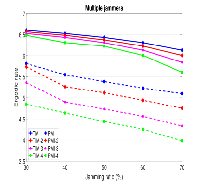
Figure 11: ER against multiple jammers.

and cumulative distribution function (CDF)

$$F(x)=\frac{1}{\Gamma(m)}\gamma(m,\frac{mx}{\lambda})=1-\frac{1}{\Gamma(m)}\Gamma(m,\frac{mx}{\lambda}),$$ (16)

where $\gamma(\cdot,\cdot)$ and $\Gamma(\cdot,\cdot)$ are the lower incomplete gamma and upper incomplete gamma functions, respectively. Since $|h_{kc_{k}}|^{2}$ has the highest channel gain among all the $L-\upsilon$ channels, the CDF of $|h_{kc_{k}}|^{2}$ is given by

$$F_{h_{kc_{k}}}(x)=\left(\frac{1}{\Gamma(m)}\gamma(m,\frac{mx}{\lambda})\right)^{(L-\upsilon)}.$$ (17)

Integrating by parts, (14) becomes

$$R_{ek}=\frac{\Omega_{k}}{\delta^{2}\ln{2}}\int_{0}^{\infty}\frac{1-F_{h_{kc_{k}}}}{1+\frac{\Omega_{k}x}{\delta^{2}}}dx.$$ (18)

Substituting $\left(\frac{1}{\Gamma(m)}\gamma(m,\frac{mx}{\lambda})\right)^{(L-\upsilon)}$ into $F_{h_{kc_{k}}}$ in (LABEL:eq51) completes the proof.

Appendix B Proof of Proposition 2

The proof of Proposition 2 is similar to that of Proposition 1 with the only difference that the channel $h_{kc_{k}}$ is chosen randomly. Thus, the PDF and CDF of $x=|h_{kc_{k}}|^{2}$ follow (15) and (16), respectively. Substitution the CDF of $x$ into (LABEL:eq5) leads to

$$R^{\prime}_{ek}=\frac{\Omega_{k}}{\delta^{2}\Gamma(m)\ln{2}}\int_{0}^{\infty}\frac{\Gamma(m,\frac{mx}{\lambda})}{1+\frac{\Omega_{k}x}{\delta^{2}}}dx,$$ (19)

and since $\frac{1}{1+\frac{\Omega_{k}x}{\delta^{2}}}=G_{1,1}^{1,1}\left(\frac{\Omega_{k}x}{\delta^{2}}\bigg{|}\begin{matrix}0\\ 0\end{matrix}\right)$ [28, Eq. (8.4.2.5)] and $\Gamma(m,\frac{mx}{\lambda})=G_{2,0}^{1,2}\left(\frac{m}{\lambda}x\bigg{|}\begin{matrix}1\\ 0,m\end{matrix}\right)$ [28, Eq. (8.4.16.2)], (LABEL:eq5) can be rewritten as

$$R^{\prime}_{ek}=\frac{\Omega_{k}\int_{0}^{\infty}G_{1,1}^{1,1}\left(\frac{\Omega_{k}x}{\delta^{2}}\bigg{|}\begin{matrix}0\\ 0\end{matrix}\right)G_{1,2}^{2,0}\left(\frac{m}{\lambda}x\bigg{|}\begin{matrix}1\\ 0,m\end{matrix}\right)dx}{\delta^{2}\Gamma(m)\ln{(2)}}.$$ (20)

By using the relationship in [29, Eq. (7.811)], (7) can be obtained, which completes the proof of Proposition 2.

References

- [1] A. Pourranjbar, G. Kaddoum, and W. Saad, “Jamming pattern recognition over multi-channel networks: A deep learning approach,” arXiv preprint arXiv:2112.11222, 2021.
- [2] Y. Xuan, Y. Shen, N. P. Nguyen, and M. T. Thai, “A trigger identification service for defending reactive jammers in WSN,” IEEE Trans Mob Comput, vol. 11, no. 5, pp. 793–806, May. 2011.
- [3] S. Nan, S. Brahma, C. A. Kamhoua, and N. O. Leslie, “Mitigation of jamming attacks via deception,” in Proc. of IEEE International Symposium on Personal, Indoor and Mobile Radio Communications. London, United Kingdom, Aug., pp. 1–6.
- [4] A. Pourranjbar, G. Kaddoum, A. Ferdowsi, and W. Saad, “Reinforcement learning for deceiving reactive jammers in wireless networks,” IEEE Trans. Commun., pp. 1–1, Mar. 2021.
- [5] S. d’Oro, L. Galluccio, G. Morabito, S. Palazzo, L. Chen, and F. Martignon, “Defeating jamming with the power of silence: A game-theoretic analysis,” IEEE Trans. Wireless Commun., vol. 14, no. 5, pp. 2337–2352, Dec. 2014.
- [6] F. Slimeni, B. Scheers, Z. Chtourou, V. L. Nir, and R. Attia, “A modified q-learning algorithm to solve cognitive radio jamming attack,” International Journal of Embedded Systems, vol. 10, no. 1, pp. 41–51, 2018.
- [7] F. Yao and L. Jia, “A collaborative multi-agent reinforcement learning anti-jamming algorithm in wireless networks,” IEEE Wireless Commun. Lett., vol. 8, no. 4, pp. 1024–1027, 2019.
- [8] I. Elleuch, A. Pourranjbar, and G. Kaddoum, “A novel distributed multi-agent reinforcement learning algorithm against jamming attacks,” IEEE Commun. Lett., 2021.
- [9] Q. Qu, S. Wei, S. Liu, J. Liang, and J. Shi, “Jrnet: Jamming recognition networks for radar compound suppression jamming signals,” IEEE Transactions on Vehicular Technology, vol. 69, no. 12, pp. 15 035–15 045, 2020.
- [10] G. Shao, Y. Chen, and Y. Wei, “Convolutional neural network-based radar jamming signal classification with sufficient and limited samples,” IEEE Access, vol. 8, pp. 80 588–80 598, Dec. 2020.
- [11] Z. Wu, Y. Zhao, Z. Yin, and H. Luo, “Jamming signals classification using convolutional neural network,” in Proc. IEEE International Symposium on Signal Processing and Information Technology (ISSPIT). Bilbao, Spain, June. 2017, pp. 062–067.
- [12] Y. Wang, B. Sun, and N. Wang, “Recognition of radar active-jamming through convolutional neural networks,” The Journal of Engineering, vol. 2019, no. 21, pp. 7695–7697, 2019.
- [13] Y. Cai, K. Shi, F. Song, Y. Xu, X. Wang, and H. Luan, “Jamming pattern recognition using spectrum waterfall: A deep learning method,” in 2019 IEEE 5th International Conference on Computer and Communications (ICCC). Chengdu, China, Dec. 2019, pp. 2113–2117.
- [14] A. Garnaev, A. Petropulu, W. Trappe, and H. V. Poor, “A multi-jammer game with latency as the user’s communication utility,” IEEE Commun. Lett., vol. 24, no. 9, pp. 1899–1903, 2020.
- [15] ——, “A multi-jammer power control game,” IEEE Commun. Lett., vol. 25, no. 9, pp. 3031–3035, 2021.
- [16] N. Van Huynh, D. T. Hoang, D. N. Nguyen, E. Dutkiewicz, and M. Mueck, “Defeating smart and reactive jammers with unlimited power,” in Proc. of IEEE Wireless Communications and Networking Conference. Seoul, South Korea, May 2020, pp. 1–6.
- [17] I. Lotfi, D. Niyato, S. Sun, H. T. Dinh, Y. Li, and D. I. Kim, “Protecting multi-function wireless systems from jammers with backscatter assistance: An intelligent strategy,” IEEE Trans. Veh. Technol., vol. 70, no. 11, pp. 11 812–11 826, 2021.
- [18] V. Le Nir and B. Scheers, “Multiple jammer localization and transmission power estimation for radio environment map,” in International Conference on Military Communications and Information Systems (ICMCIS). Warsaw, Poland, May. 2018, pp. 1–5.
- [19] S. Bhamidipati and G. X. Gao, “Simultaneous localization of multiple jammers and receivers using probability hypothesis density,” in 2018 IEEE/ION Position, Location and Navigation Symposium (PLANS). Monterey, CA, USA, Apr. 2018, pp. 940–944.
- [20] M. Juhlin and A. Jakobsson, “Localization of multiple jammers in wireless sensor networks,” in 2021 29th European Signal Processing Conference (EUSIPCO). Dublin, Ireland, Aug 2021, pp. 1596–1600.
- [21] Z. Li, Y. Lu, X. Li, Z. Wang, W. Qiao, and Y. Liu, “Uav networks against multiple maneuvering smart jamming with knowledge-based reinforcement learning,” IEEE Internet Things J., 2021.
- [22] Y. Wu, W. Yang, X. Guan, and Q. Wu, “Energy-efficient trajectory design for uav-enabled communication under malicious jamming,” IEEE Wireless Commun. Lett., vol. 10, no. 2, pp. 206–210, 2020.
- [23] Y. Wu, X. Guan, W. Yang, and Q. Wu, “Uav swarm communication under malicious jamming: Joint trajectory and clustering design,” IEEE Wireless Commun. Lett., vol. 10, no. 10, pp. 2264–2268, 2021.
- [24] B. Gingras, A. Pourranjbar, and G. Kaddoum, “Collaborative spectrum sensing in tactical wireless networks,” in 2020 IEEE ICC. Dublin, Ireland, Jun. 2020, pp. 1–6.
- [25] J. Lundén, M. Motani, and H. V. Poor, “Distributed algorithms for sharing spectrum sensing information in cognitive radio networks,” IEEE Trans. Wireless Commun., vol. 14, no. 8, pp. 4667–4678, 2015.
- [26] K. Cho, B. Van Merriënboer, C. Gulcehre, D. Bahdanau, F. Bougares, H. Schwenk, and Y. Bengio, “Learning phrase representations using rnn encoder-decoder for statistical machine translation,” arXiv preprint arXiv:1406.1078, 2014.
- [27] J. Chung, C. Gulcehre, K. Cho, and Y. Bengio, “Empirical evaluation of gated recurrent neural networks on sequence modeling,” arXiv preprint arXiv:1412.3555, 2014.
- [28] A. Prudnikov, Y. Brychkov, and O. Marichev, Integrals and Series, Volume 3: More Special Functions. Boca Raton, FL, USA: CRC Press, 1999.
- [29] I. S. Gradshteyn and I. M. Ryzhik, Tables of Integrals, Series, and Products, 7th ed. New York, NY, USA: Academic Press, 2007.