Sampling-Dependent Transition Paths of Iceland–Scotland Overflow Water

Abstract

In this note, we apply Transition Path Theory (TPT) from Markov chains to shed light on the problem of Iceland–Scotland Overflow Water (ISOW) equatorward export. A recent analysis of observed trajectories of submerged floats demanded revision of the traditional abyssal circulation theory, which postulates that ISOW should steadily flow along a deep boundary current (DBC) around the subpolar North Atlantic prior to exiting it. The TPT analyses carried out here allow to focus the attention on the portions of flow from the origin of ISOW to the region where ISOW exits the subpolar North Atlantic and suggest that insufficient sampling may be biasing the aforementioned demand. The analyses, appropriately adapted to represent a continuous input of ISOW, are carried out on three time-homogeneous Markov chains modeling the ISOW flow. One is constructed using a high number of simulated trajectories homogeneously covering the flow domain. The other two use much fewer trajectories which heterogeneously cover the domain. The trajectories in the latter two chains are observed trajectories or simulated trajectories subsampled at the observed frequency. While the densely sampled chain supports a well-defined DBC, the more heterogeneously sampled chains do not, irrespective of whether observed or simulated trajectories are used. Studying the sampling sensitivity of the Markov chains, we can give recommendations for enlarging the existing float dataset to improve the significance of conclusions about time-asymptotic aspects of the ISOW circulation.

1 Introduction

The strength of the Atlantic Meridional Overturning Circulation (AMOC) and its impact on global climate through heat and freshwater transport is linked to the rates of formation of North Atlantic Deep Water (NADW) (Buckley and Marshall, 2016). Representing the lower limb of the AMOC, the NADW flows southward.

The Greenland–Scotland Ridge is a region shallower than 500 m, which separates the Nordic seas from the subpolar North Atlantic (Fig. 1). The overflow of dense water across that ridge entrains the thermocline and mid-depth water, representing one deep-water formation process (Daniault et al., 2016). The Iceland–Scotland Overflow Water (ISOW) is the lighter of the two overflow components of NADW. It enters the Iceland Basin mainly through the Faroe Bank Channel and channels across the Iceland–Faroe Ridge, at a volumetric flow rate of about 5 Sv (1 Sv = 10⁶ m³ s^-1). The ISOW is characterized by potential (i.e., with adiabatic heating effects removed) temperature in the range $-1^{\circ}\text{C}<T_{\theta}<2.5^{\circ}\text{C}$ and salinity (salt fraction times $10^{-3}$, approximately) in the tight interval $34.9<S<34.97$. These $T_{\theta}$ and $S$ values roughly correspond to potential sigma-density (density in kg m^-3 minus $10^{3}$, as is most commonly used in oceanography) in the narrow range $27.8\text{ kg\,m}^{-3}<\sigma_{\theta}<27.9\text{ kg\,m}^{-3}$, which is typically found within 1600–2600 m. This characterization of ISOW follows Johns et al. (2021), and is supported by in-situ data collected during the Overturning in the Subpolar North Atlantic Program (OSNAP) (Lozier et al., 2017). In-situ observations of the ISOW plume date back to at least the mid 20th century (Steele et al., 1962); cf. Johns et al. (2021) for a quite detailed account on the observational efforts that followed.

The heavier overflow component of NADW is the Denmark Strait Overflow Water (DSOW), which enters the Irminger Basin between Greenland and Iceland. This component is not of our interest here.

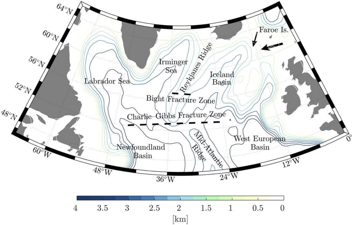
Figure 1: The subpolar North Atlantic domain of interest with main geographic features indicated. The ISOW enters the Iceland Basin primarily through the Faroe Bank Channel (thick arrow) and channels across the Iceland–Faroe Ridge (thin arrow). In blue tones, selected isobaths.

The traditional theory of large-scale abyssal circulation of the ocean postulates that ISOW should steadily flow equatorward, forming a deep boundary current (DBC) around the subpolar North Atlantic (Stommel, 1958). The trajectories of 21 acoustically-tracked isobaric RAFOS (Range and Fixing of Sound) floats (Rossby et al., 1986), deployed at 1800–2800 m depth as part of OSNAP, challenge this traditional view, according to Zou et al. (2020). By contrast, they suggest the existence of multiple equatorward ISOW paths, which represents a puzzle. A similarly puzzling assessment was made by Zou et al. (2020) from the inspection of simulated float trajectories of the same duration (up to 2 years) as, and also longer (10 years) than, the observed trajectories. In arriving at their conclusions, Zou et al. (2020) employed direct inspection of individual observed float trajectories and the construction of probability distributions (histograms) of observed and simulated float positions.

The recent application by Miron et al. (2022) of Transition Path Theory (TPT) (E and Vanden-Eijnden, 2006; Metzner et al., 2009; Helfmann et al., 2020) to the discretized motion of all available submerged floats (over 250, of RAFOS and of other type, with the RAFOS floats corresponding to the totality of those deployed during OSNAP) represents an attempt to resolve the above puzzle. TPT highlights the dominant pathways of fluid parcels connecting a chosen source with a target region of the flow domain. That is, instead of studying the individual complicated paths connecting source with target, TPT concerns their average behaviour and shows their dominant transition channels. Thus TPT leads to a much cleaner picture, and is hence much easier to interpret than probability distributions computed using the raw trajectories as in Zou et al. (2020). Moreover, the framework for TPT is given by a Markov chain model, which is constructed from short-run trajectories. This is advantageous when dealing with observed trajectories, even when records might seem too brief to make long-term transport assessments. Indeed, under a stationarity assumption, which is appropriate to study abyssal circulation due to its slow evolution, asymptotic aspects of the Lagrangian dynamics can be robustly framed by Markov Chains. By contrast, long trajectory integrations of numerically produced velocity data, as carried out in Zou et al. (2020), are sensitively dependent on initial conditions and hence subject to exponential divergence with time, making long-term transport assessments dubious.

Miron et al. (2022) found that transition paths of floats can organize along a DBC, consistent with traditional abyssal circulation theory. However, their results are not strictly conclusive for ISOW as they considered floats in a depth range where the heavier overflow component of NADW (the DSOW) is also present.

We revisit the problem of the ISOW export paths from the subpolar North Atlantic by applying TPT on observed float trajectories restricted to a depth range within which ISOW is expected to be better constrained. We also consider simulated float trajectories, but along an isopycnic (constant density) layer that intersects the ISOW density range. TPT (reviewed in Section 2) is appropriately adapted (in Section 3) to include the effects of a continuous injection of ISOW into the subpolar North Atlantic, which represents a further improvement over Miron et al. (2022). This is done by imposing a mass balance (of ISOW) within the open ocean domain of interest, which requires one to use a recent adaptation of TPT to open dynamical systems (Miron et al., 2021). An important result, among other characterizations of the ISOW problem (cf. Section 4) is that insufficient sampling of the flow domain may mask the presence of a DBC of ISOW. Section 5 is dedicated to investigate the robustness of this result. The paper is finalized with a summary and some concluding remarks with recommendations on how to circumvent the sampling issue (Section 6).

2 Transition path theory

Suppose that the long-term motion of fluid parcels can be described by a stationary stochastic (advection–diffusion) process. Upon an appropriate spatiotemporal discretization of the Lagrangian dynamics, fluid parcels evolve like random walkers of an autonomous, discrete-time Markov chain. That is, conditional on the current location of the fluid parcel, the Markov chain assigns to each possible next location a certain transition probability. Such a discretization into spatial boxes and discrete time steps can be achieved using Ulam’s method (e.g., Koltai, 2010), by projecting probability densities onto a finite-dimensional vector space spanned by indicator functions on boxes, which, covering the flow domain, are normalized by their Lebesgue measure (area) (Miron et al., 2019b). The spatial boxes represent the locations or states of the chain.

Thus, if $X_{n}$ denotes the random position at discrete time $nT$, $n\in\mathbb{Z}$, on a closed two-dimensional flow domain $\mathcal{D}$ covered by $N$ disjoint boxes $\{B_{1},\dotsc,B_{N}\}=:\mathcal{D}_{N}$, then $\operatorname{prob}(X_{n+1}\in B_{j})=\sum_{i:B_{i}\in\mathcal{D}_{N}}P_{ij}\operatorname{prob}(X_{n}\in B_{i})$ where

$$P_{ij}:=\operatorname{prob}(X_{n+1}\in B_{j}\mid X_{n}\in B_{i}),\quad\sum_{j:B_{j}\in\mathcal{D}_{N}}P_{ij}=1,$$ (1)

is the one-step conditional probability of transitioning between $B_{i}$ and $B_{j}$. The row-stochastic matrix (i.e., with nonnegative entries and whose rows sum to one) $\smash{P=(P_{ij})_{i,j:B_{i},B_{j}\in\mathcal{D}_{N}}\in\mathbb{R}^{N\times N}}$ is called the transition matrix of the Markov chain $\{X_{n}\}_{n\in\mathbb{Z}}$.

Let $x(t)$ represent a very long stationary fluid parcel trajectory visiting every box of the covering of $\mathcal{D}$ many times. Then $x_{0}:=x(t)$ and $x_{T}:=x(t+T)$ at any $t>0$ provide observations for $X_{n}$ and $X_{n+1}$, respectively. These can be used to approximate $P_{ij}$ via counting transitions between boxes, viz.,

$$P_{ij}\approx\frac{C_{ij}}{\sum_{l:B_{l}\in\mathcal{D}_{N}}C_{il}}$$ (2a)

where

$$C_{ij}:=\#\big{\{}x(t)\in B_{i},\,x(t+T)\in B_{j},\,t:\text{any}\big{\}}.$$ (2b)

If $P$ is irreducible or ergodic (i.e., all states in the Markov chain communicate) and aperiodic or mixing (i.e., no state is revisited cyclically), its dominant left eigenvector, $\bm{\pi}$, satisfies $\bm{\pi}P=\bm{\pi}$, and can be chosen componentwise positive. Scaled appropriately it represents a (limiting, invariant) stationary distribution, namely, $\bm{\pi}=\smash{\lim_{k\uparrow\infty}\mathbf{f}P^{k}}$ for any probability vector $\mathbf{f}$ (Norris, 1998). We will assume that the Markov chain is in stationarity, meaning that $\operatorname{prob}(X_{n}\in B_{i})=\pi_{i}$ for all $n\in\mathbb{Z}$.

Transition Path Theory (TPT) provides a rigorous characterization of the ensemble of trajectory pieces, which, flowing out last from a region $\mathcal{A}\subset\mathcal{D}_{N}$, next go to a region $\mathcal{B}\subset\mathcal{D}_{N}$, disconnected from $\mathcal{A}$. Such trajectory pieces are called reactive trajectories due to tradition originated in chemistry, which identifies $\mathcal{A}$ resp. $\mathcal{B}$ with the reactant resp. product of a chemical reaction. In fluidic terms, reactive trajectories most effectively contribute to the transport between $\mathcal{A}$ and $\mathcal{B}$, which will herein be referred to as source and target, respectively.

The main objects of TPT are the forward committor probability, $\smash{\mathbf{q}^{+}=(q^{+}_{i})_{i:B_{i}\in\mathcal{D}_{N}}}$, giving the probability of a trajectory initially in box $B_{i}$ to first enter the target $\mathcal{B}$ and not the source $\mathcal{A}$, and the backward committor probability, $\smash{\mathbf{q}^{-}=(q^{-}_{i})_{i:B_{i}\in\mathcal{D}_{N}}}$, giving the probability of a trajectory in box $B_{i}$ to have last exit the source $\mathcal{A}$ and not the target $\mathcal{B}$. The committors are fully computable from $P$ and $\bm{\pi}$, according to (Metzner et al., 2009; Helfmann et al., 2020):

$$\left\{\begin{aligned} &{\left.\kern-1.2pt\mathbf{q}^{\pm}\right|_{\mathcal{D}_{N}\setminus(\mathcal{A}\cup\mathcal{B})}}={\left.\kern-1.2ptP^{\pm}\right|_{\mathcal{D}_{N}\setminus\mathcal{A}\cup\mathcal{B},\mathcal{D}_{N}}}\mathbf{q}^{\pm},\\ &{\left.\kern-1.2pt\mathbf{q}^{+}\right|_{\mathcal{A}}}=\mathbf{0}^{|\mathcal{A}|\times 1},\quad{\left.\kern-1.2pt\mathbf{q}^{-}\right|_{\mathcal{B}}}=\mathbf{0}^{|\mathcal{B}|\times 1},,\\ &{\left.\kern-1.2pt\mathbf{q}^{+}\right|_{\mathcal{B}}}=\mathbf{1}^{|\mathcal{B}|\times 1},\quad{\left.\kern-1.2pt\mathbf{q}^{-}\right|_{\mathcal{A}}}=\mathbf{1}^{|\mathcal{A}|\times 1}.\end{aligned}\right.$$ (3)

Here, ${\left.\kern-1.2pt\right|_{\mathcal{S}}}$ denotes restriction to the set $\mathcal{S}$ while ${\left.\kern-1.2pt\right|_{\mathcal{S},\mathcal{S}^{\prime}}}$ that to rows corresponding to $\mathcal{S}$ and columns to $\mathcal{S}^{\prime}$; $P^{+}=P$; and

$$P^{-}_{ij}:=\operatorname{prob}(X_{n}\in B_{j}\mid X_{n+1}\in B_{i})=\frac{\pi_{j}}{\pi_{i}}P_{ji}$$ (4)

are the entries of the time-reversed transition matrix, i.e., for the original chain traversed in backward time, $\{X_{-n}\}_{n\in\mathbb{Z}}$.

The committor probabilities are used to express several statistics of the ensemble of reactive trajectories as follows (Helfmann et al., 2020):

• The reactive distribution, $\smash{\bm{\pi}^{\mathcal{A}\mathcal{B}}=(\pi^{\mathcal{A}\mathcal{B}}_{i})_{i:B_{i}\in\mathcal{D}_{N}}}$, where $\pi^{\mathcal{A}\mathcal{B}}_{i}$ is defined as the joint probability that a trajectory is in box $B_{i}$ while transitioning from $\mathcal{A}$ to $\mathcal{B}$ and is computable as

  $$\pi^{\mathcal{A}\mathcal{B}}_{i}=q^{-}_{i}\pi_{i}q^{+}_{i}.$$ (5)

• The reactive currents, $\smash{f^{+}=(f^{+}_{ij})_{i,j:B_{i},B_{j}\in\mathcal{D}_{N}}}$, where $f^{+}_{ij}$ gives the net flux of trajectories going through $B_{i}$ at time $nT$ and $B_{j}$ at time $(n+1)T$ on their way from $\mathcal{A}$ to $\mathcal{B}$, indicates the dominant transition channels. This is computable according to

  $$f^{+}_{ij}:=\max\left\{f^{\mathcal{A}\mathcal{B}}_{ij}-f^{\mathcal{A}\mathcal{B}}_{ji},0\right\},\quad f^{\mathcal{A}\mathcal{B}}_{ij}=q^{-}_{i}\pi_{i}P_{ij}q^{+}_{j}.$$ (6)

• The reactive rate of trajectories leaving $\mathcal{A}$ resp. entering $\mathcal{B}$, defined as the probability per time step of a reactive trajectory to leave $\mathcal{A}$ resp. enter $\mathcal{B}$, is computed as

  $$k^{\mathcal{A}\to\mathcal{B}}:=\sum_{\begin{subarray}{c}i:B_{i}\in\mathcal{A},\\ j:B_{j}\in\mathcal{D}_{N}\end{subarray}}f^{\mathcal{A}\mathcal{B}}_{ij}\text{ resp.\ }k^{\mathcal{B}\leftarrow\mathcal{A}}:=\sum_{\begin{subarray}{c}i:B_{i}\in\mathcal{D}_{N},\\ j:B_{j}\in\mathcal{B}\end{subarray}}f^{\mathcal{A}\mathcal{B}}_{ij},$$ (7)

  and gives the proportion of reactive trajectories leaving $\mathcal{A}$ resp. entering $\mathcal{B}$. It turns out that

  $$k^{\mathcal{A}\to\mathcal{B}}\equiv k^{\mathcal{B}\leftarrow\mathcal{A}}=:k^{\mathcal{A}\mathcal{B}}.$$ (8)

  In some situations, as we consider below, it is insightful to further decompose the transition rate

  $$k^{\mathcal{B}\leftarrow\mathcal{A}}=\sum_{j:B_{j}\in\mathcal{B}}k^{B_{j}\leftarrow\mathcal{A}}$$ (9)

  into the individual arrival rates into the disjoint boxes $B_{j}$ that cover $\mathcal{B}$:

  $$k^{B_{j}\leftarrow\mathcal{A}}=\sum_{i:B_{i}\in\mathcal{D}_{N}}f^{AB}_{ij}.$$ (10)

  The same can be done for decomposing $k^{\mathcal{A}\to\mathcal{B}}$.

• Finally, the reaction duration, $t^{\mathcal{A}\mathcal{B}}$, of a transition from $\mathcal{A}$ to $\mathcal{B}$ is obtained by dividing the probability of being reactive by the transition rate interpreted as a frequency, viz.,

  $$t^{\mathcal{A}\mathcal{B}}:=\frac{\sum_{i:B_{i}\in\mathcal{D}_{N}}\pi^{\mathcal{A}\mathcal{B}}_{i}}{k^{\mathcal{A}\mathcal{B}}}.$$ (11)

3 The ISOW problem

For the ISOW problem, we are interested in the source set given by the region where ISOW originates and a target set given by the area where ISOW exits the subpolar North Atlantic. Since the domain $\mathcal{D}$ here represents a subdomain of the subpolar North Atlantic, and thus an open flow domain, $P$ cannot be row-stochastic, which requires an adaptation of TPT. This is proposed in Miron et al. (2021), which we further adapt here to account for the input of ISOW into $\mathcal{D}$.

Specifically, we replace $P$ by a row-stochastic transition matrix $\tilde{P}\in\mathbb{R}^{(N+1)\times(N+1)}$ defined by

$$\tilde{P}:=\begin{pmatrix}P&P^{\mathcal{D}_{N}\to\omega}\\ P^{\mathcal{A}\leftarrow\omega}&0\end{pmatrix}$$ (12)

on the extended domain $\mathcal{D}_{N}\cup\omega.$ Here, $\omega$ denotes a state, called a two-way nirvana state, which is added to the chain defined by $P$. It absorbs probability imbalance from $\mathcal{D}_{N}$, which is sent back to the chain through the source $\mathcal{A}$. More precisely, in (12),

$$P^{\mathcal{D}_{N}\to\omega}=\Big{(}1-\sum\nolimits_{j:B_{j}\in\mathcal{D}_{N}}P_{ij}\Big{)}_{i:B_{i}\in\mathcal{D}_{N}}\in\mathbb{R}^{N\times 1}$$ (13)

gives the outflow from $\mathcal{D}_{N}$ and

$$P^{\mathcal{A}\leftarrow\omega}=\frac{\mathbf{1}_{\mathcal{A}}}{|\mathcal{A}|}\in\mathbb{R}^{1\times N}$$ (14)

is a probability vector that gives the inflow into $\mathcal{D}_{N}$, taken to take place uniformly through $\mathcal{A}$, thereby enforcing a mass balance for ISOW. In other words, this guarantees a continuous inflow of ISOW through $\mathcal{A}$, whose transition paths into the target $\mathcal{B}$, to be placed at the southern edge of the subpolar North Atlantic (sub)domain $\mathcal{D}_{N}$, can be unequivocally tracked.

TPT is adapted in Miron et al. (2021) such that transitions between $\mathcal{A}$ and $\mathcal{B}$ are constrained to take place within $\mathcal{D}_{N}$, i.e., they avoid the artificial state $\omega$. This is shown in Miron et al. (2021) to be accomplished by restricting the committor problem to $\mathcal{D}_{N}$. The restricted committor equations are given by (3) with the substochastic matrix $P^{+}_{ij}=P_{ij}$ on the open domain $\mathcal{D}_{N}$ and the replacement $P^{-}_{ij}=\smash{\frac{\tilde{\pi}_{j}}{\tilde{\pi}_{i}}P_{ji}}$ for $i,j:B_{i},B_{j}\in\mathcal{D}_{N}$. That is, the transition matrix for the open time-reversed Markov chain is computed using the restriction to $\mathcal{D}_{N}$ of $\tilde{\bm{\pi}}$, the stationary distribution of the closed transition matrix $\tilde{P}$. Since the probability imbalance enters the open domain via $\mathcal{A}$, the transition paths that avoid $\omega$ are unaffected by this artificial closure of the system. The rest of the TPT formulae remain the same, except that for computing the statistics, $\bm{\pi}$ is replaced by ${\left.\kern-1.2pt\tilde{\bm{\pi}}\right|_{\mathcal{D}_{N}}}$.

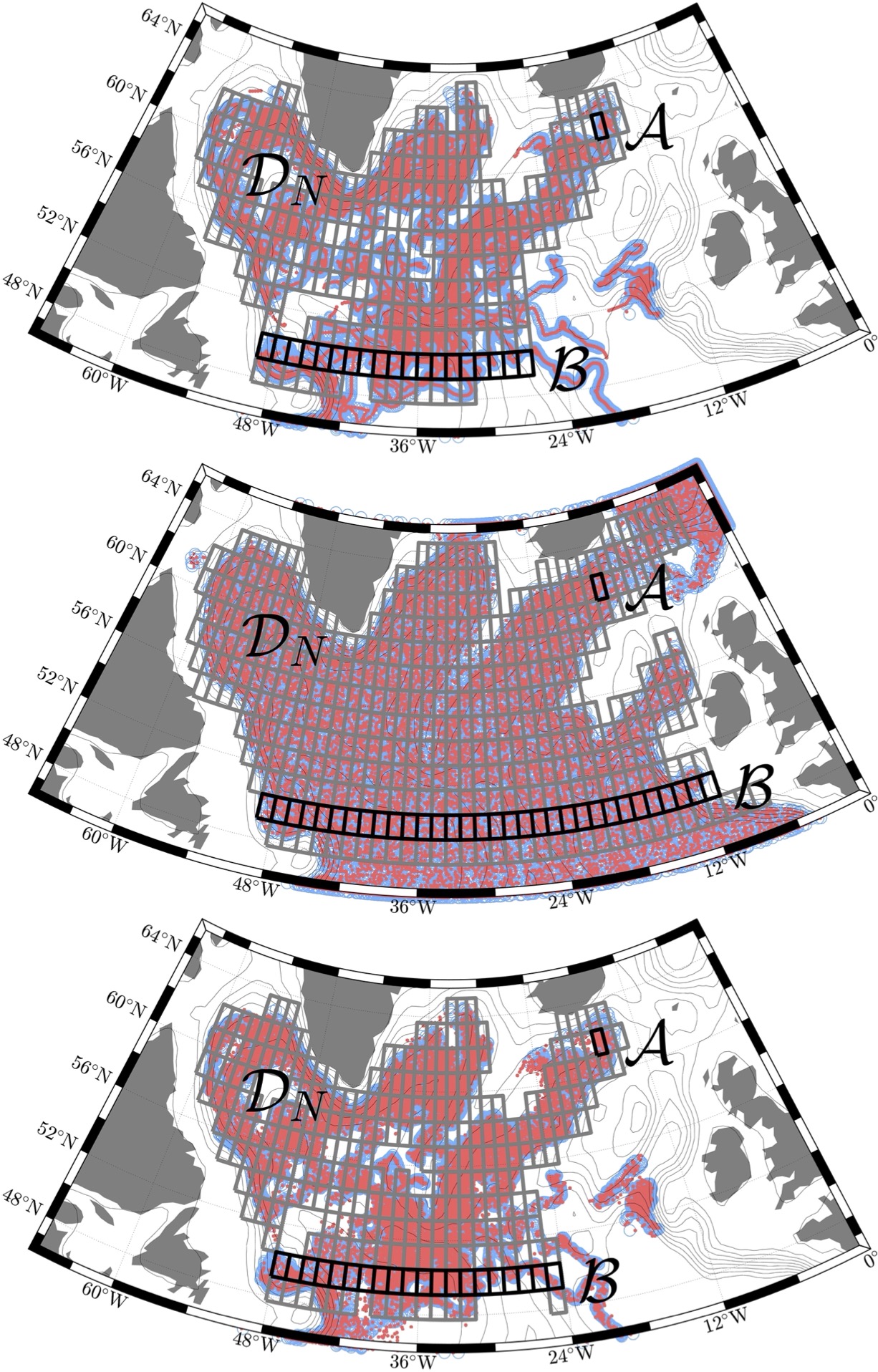
Figure 2: (top panel) Ignoring the start date, initial positions $x_{0}$ (light blue) and positions after 10 days $x_{T}$ (light red) of available acoustically-tracked RAFOS and satellite-tracked profiling Argo floats parked between 1600 and 2600 m, where ISOW is typically found. In thick gray, boxes of the domain covering ($\mathcal{D}_{N}$) used to construct a maximally communicating Markov chain for TPT analysis. In black, source ($\mathcal{A}$) and target ($\mathcal{B}$) used in the TPT analysis. The thin gray curves are selected isobaths. (middle panel) As in the top panel, but based on simulated float trajectories integrated from HYCOM model velocities on an density layer intersecting the typical ISOW density range. Unlike in the top panel, the initial positions $x_{0}$ uniformly cover the flow domain. (bottom panel) As in the middle panel, but only using initial positions $x_{0}$ that lie in closest proximity to those of the observed floats.

To carry out the TPT analysis of the ISOW problem just posed, we will consider two datasets for estimating the transition matrix as in (2b). On the one hand, we have observed trajectories produced by acoustically-tracked RAFOS floats (from OSNAP and earlier experiments) and satellite-tracked profiling Argo floats (Argo, 2000), deployed in the subpolar North Atlantic domain of interest (in the 1990s and mid-2010s), or that simply happened to travel through it (since the 1980s) (cf. Miron et al., 2022, for details of the two types of isobaric floats). Unlike in the TPT analysis of Miron et al. (2022), we restrict to trajectories parked between 1600 and 2600 m, a depth range where ISOW is expected to be found (Zou et al., 2020; Johns et al., 2021). There is a total of 268 float trajectories, with positions interpolated 10-daily. If a given trajectory contains a gap larger than 10 days, then it is split into two separate trajectories. The transition time choice of $T=10$ days and the box size of (roughly) 1^∘-by-1^∘ were found sufficient to allow maximal communication by the application of the Tarjan’s algorithm (Tarjan, 1972) on a time-homogeneous (as we ignore the start day of the trajectories) Markov chain on boxes over $\mathcal{D}$ that covers the largest portion of the subpolar North Atlantic (Fig. 2, top panel). We will refer to this chain as the observed chain.

On the other hand, we consider simulated float trajectories obtained by integrating velocities produced by a 1/12^∘ Atlantic Ocean simulation based on HYCOM (HYbrid-Coordinate Ocean Model), as described in Xu et al. (2013) and considered by Zou et al. (2020). The velocities were extracted (except north of the domain of interest, where interpolation was involved) on the model’s native isopycnic-coordinate level (layer) $k=26$, which intersects the ISOW typical density range. The trajectories were initialized every 5 days for 2 years from a very dense grid over the subpolar North Atlantic domain, each one lasting 60 days. Ignoring the start day and using the same transition time ($T=10$ days) as with the observed trajectories, a maximally communicating Markov chain on boxes (of the same size, 1^∘-by-1^∘, as in the case of observed trajectories) over $\mathcal{D}$ is obtained, which covers the subpolar North Atlantic as shown in the middle panel of Fig. 2. Unlike in the observed trajectory case, in which there are on average about 100 data points per box, the simulated trajectory case contains on average 1500 data points per box. We will refer to this chain as the simulated chain.

A third Markov chain is constructed, with the corresponding box covering shown in the bottom panel of Fig. 2. This uses a subset of the simulated float trajectories with $x_{0}$ chosen to lie closest to those of the observed floats. This is done to test the dependence of the TPT analysis on sampling. We will refer to this chain as the truncated chain.

The source set $\mathcal{A}$ for TPT analysis is chosen to include one box and to be located in the northernmost end of the Iceland Basin, where ISOW enters the subpolar North Atlantic. The nominal geographic location of the box is (16.37^∘W, 62.55^∘N), which slightly varies depending on the Markov chain. The target set $\mathcal{B}$ is placed along 49.25^∘N, to frame export paths of ISOW out of the subpolar North Atlantic. This is the southernmost and longest row of boxes for the three chains considered.

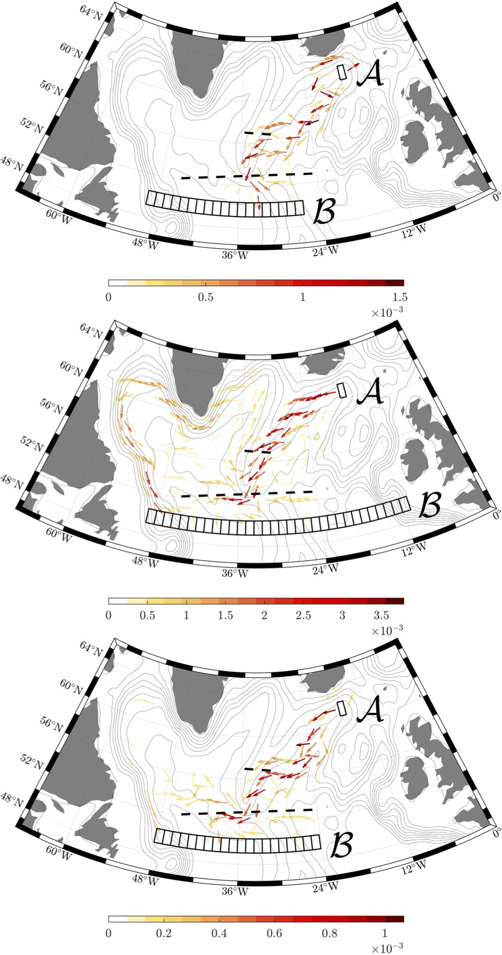
Figure 3: Reactive currents of ISOW as described by observed floats (top panel), simulated floats (middle panel), and simulated floats starting at observed float positions (bottom panel). The thin gray curves are the isobaths shown in Fig. 1. The broken straight lines indicate the Bight Fracture Zone (northern line) and the Charlie–Gibbs Fracture Zone (southern line).

4 TPT analysis of ISOW

We begin by showing in Fig. 3 the resulting reactive currents. To visualize them, we follow Helfmann et al. (2020) and for each box $B_{i}$ of the covering of $\mathcal{D}$, we estimate the vector of the average direction and magnitude of the reactive current ($f^{+}$) to other boxes $B_{j}$, $j\neq i$. In agreement with traditional abyssal circulation theory, the reactive currents out of the source in the simulated chain (Fig. 3, middle panel) organize into a DBC, which turns northward following the bathymetry of the western flank of the Reykjanes Ridge, then continues counter-clockwise around the Irminger Sea, and subsequently around of the Labrador Sea after turning northward around the southern tip of Greenland. This happens before the reactive currents reach the westernmost boxes of the target, in the Newfoundland Basin, which are also reached by reactive currents that shortcut the DBC across the Charlie–Gibbs Fracture Zone. This is in stark contrast to the reactive currents supported by the observed chain (Fig. 3, top panel), which do not reveal a DBC, but rather reach the target east of the Mid-Atlantic Ridge. The picture, however, is not too different than that one drawn by the truncated chain (Fig. 3, bottom panel), suggesting that the absence of a well-defined DBC in the observed chain might be due to insufficient sampling.

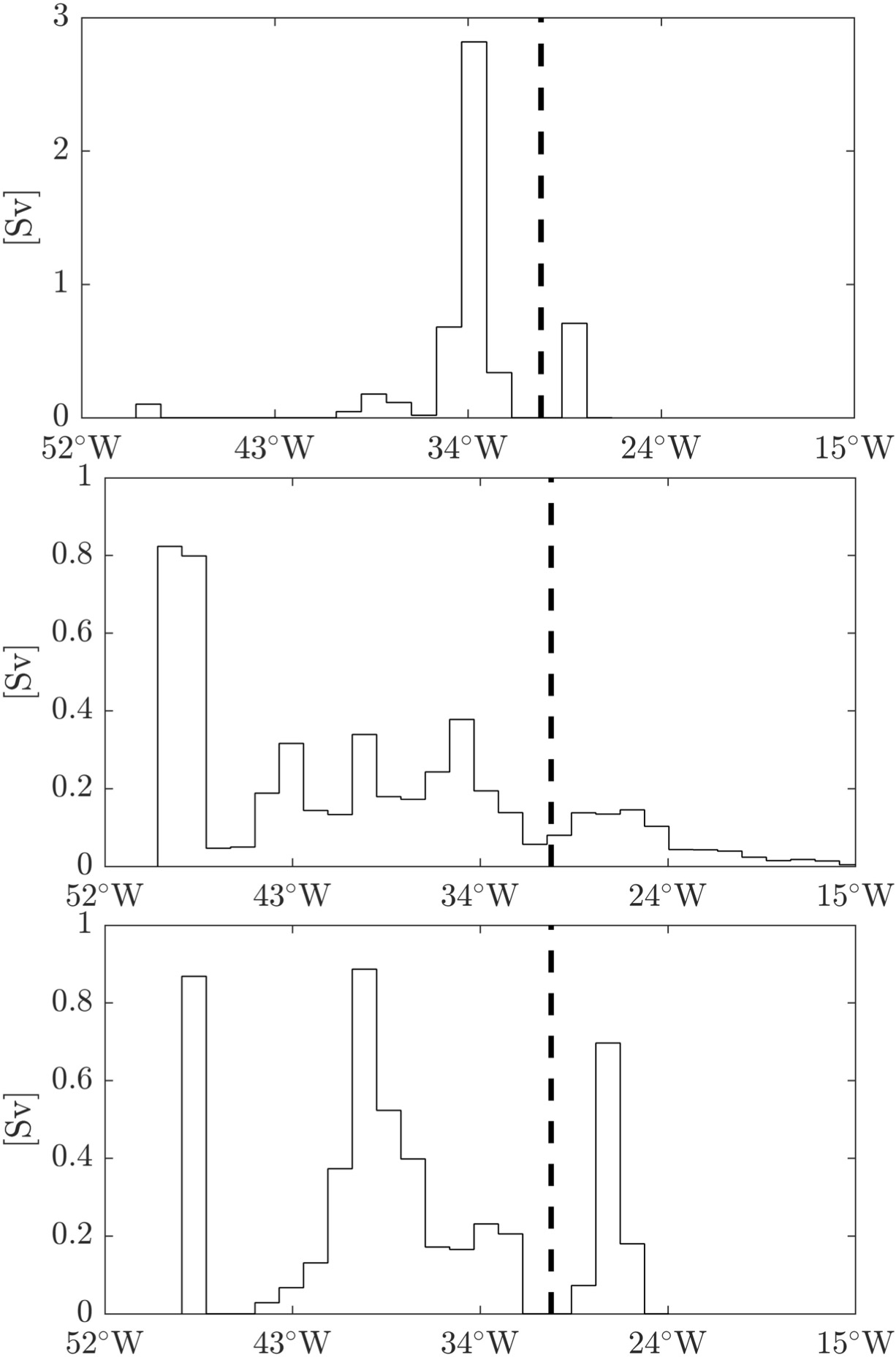
Figure 4: Reactive rates, converted into volumetric fluxes, into each of the target boxes for the Markov chain constructed using observed floats (top panel), simulated floats (middle panel), and simulated floats starting at observed float positions (bottom panel). The dashed line indicates the longitude where the target intersects the Mid-Atlantic ridge.

The reactive rates into each of the target boxes, (10), offer, as expected, a picture consistent with the reactive currents. These are depicted in Fig. 4 as a function of longitude along the target upon transforming them into volumetric flow rates. This is done by first normalizing the reactive rates into each target box by the total reactive rate into the target, and then multiplying them by the volumetric flow rate of ISOW into the subpolar North Atlantic inferred from in-situ observations (5 Sv). While in the simulated chain (Fig. 4, middle panel) the volumetric flow rate peaks in the western end of the target, in the observed chain (Fig. 4, top panel) and truncated chain (Fig. 4, bottom panel) it also peaks east of the Mid-Atlantic Ridge.

Finally, we present in Fig. 5 the domain of influence of each box of the target. This is done by associating to each domain box $B_{i}\in\mathcal{D}_{N}$ the most likely target box $B_{j}\in\mathcal{B}$ to hit according to the probability in $B_{i}\in\mathcal{D}_{N}$ to forward-commit to $B_{j}\in\mathcal{B}$ (and not to any other box in $\mathcal{B}$). This committor probability is computed using (3) for the plus sign with $P^{+}=\tilde{P}$, $\mathcal{A}=\omega\cup(\mathcal{B}\setminus B_{j})$, and $\mathcal{B}$ replaced by $B_{j}\in\mathcal{B}$. This way every box of the covering of $\mathcal{D}$ gets assigned to a target box that it will most likely reach, forming what Miron et al. (2021) have dubbed a forward-committor-based dynamical geography. Each province $\mathcal{P}\subset\mathcal{D}_{N}$ shown in Fig. 5, i.e., each set of boxes that are most likely mapped into a certain target box, is colored according to the expected exit time, $\smash{\frac{T}{1-\lambda_{\mathcal{P}}}}$, where $\lambda_{\mathcal{P}}$ is the dominant eigenvalue of $\smash{{\left.\kern-1.2pt\tilde{P}\right|_{\mathcal{P},\mathcal{P}}}}$ (e.g., Miron et al., 2019a, eq. (10)), which represents a measure of residence time in $\mathcal{P}$. The geographies are consistent with the reactive currents in Fig. 3 and the volumetric volume rates in Fig. 4. The observed chain (Fig. 5, top panel) reveals a marked partition, with the Irminger and Labrador Seas and Newfoundland Basin predominantly forward committing to the westernmost end of the target, and the Iceland Basin to a target box flanking the Mid-Atlantic Ridge on the west. Moreover, the Irminger and Labrador Seas and Newfoundland Basin have a shorter residence time (about 2 yr) compared to that of the Iceland Basin (about 14 yr). Altogether, this suggests that the Irminger and Labrador Seas and Newfoundland Basin are dynamically disconnected from the Iceland Basin. This is consistent with the absence of a DBC for the reactive currents emerging from the northern Iceland Basin. By contrast, in the simulated chain (Fig. 5, middle panel) the Iceland Basin is forward committed to the western side of the target and has a residence time comparable to that of the Irminger and Labrador Seas and Newfoundland Basin (2 to 5 yr, overall). This suggests a dynamical connection of the Iceland Basin with the Irminger and Labrador Seas and Newfoundland Basin, enabling, as a consequence, reactive currents starting in the northern Iceland Basin to develop a DBC. But for the truncated chain (Fig. 5, bottom panel), the Iceland Basin presents a similar lack of communication with the Irminger and Labrador Seas and Newfoundland Basin as in the observed chain, highlighting the possibility that insufficient sampling by floats may be masking the emergence of a DBC of ISOW.

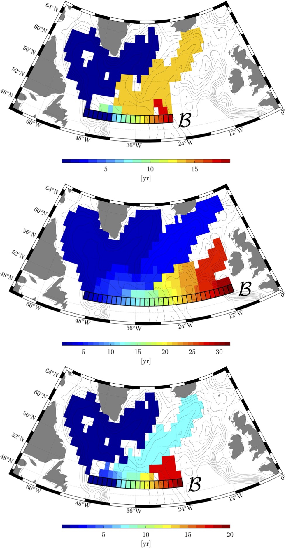
Figure 5: Forward-committor-based dynamical geography revealing domains of influence for each box of the target with the provinces colored according to residence time for the observed (top panel), simulated (middle panel), and truncated (bottom panel) Markov chain. The gray curves are the isobaths shown in Fig. 1.

5 Testing the sampling sensitivity

The conclusion above on insufficient sampling deserves further consideration. In what follows we first test its robustness by considering the results from reducing uniformly at random the number of simulated trajectories $(x_{0},x_{T})$ involved in the construction of the simulated Markov chain until it agrees with the amount in the truncated chain. Figure 6 shows the results for the computation of the reactive rates into the target boxes at the southern edge of the domain. The circles are averages over 100 uniform random reductions of the trajectories by 93%. These averages are accompanied by one-standard-deviation error bars. Overlaid in blue is the reactive rate obtained using the simulated Markov chain computed using all trajectories at disposal. As can be seen, this result is surprisingly very robust, given that only 7% of the trajectories are considered. By contrast, the reactive rates obtained using the truncated Markov chain (red curve in Fig. 6) are quite different and lie nearly everywhere outside of the variability of the rates of the uniformly reduced Markov chain, even though it uses approximately the same amount of trajectories.

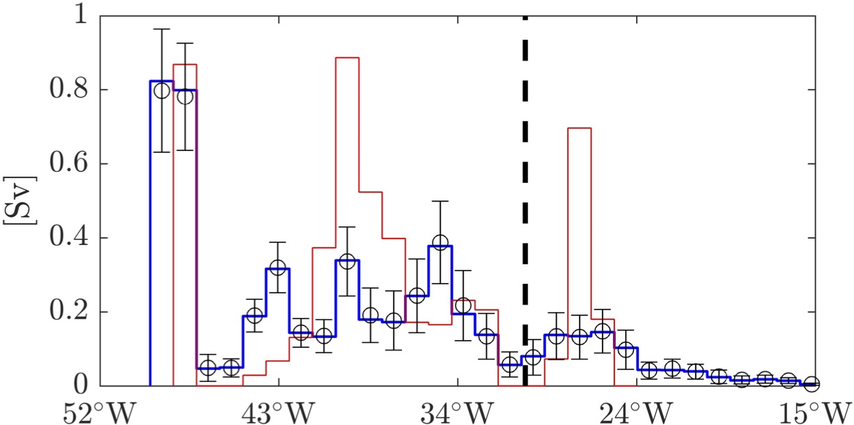
Figure 6: As in Fig. 4, but for the simulated Markov chain after reducing uniformly at random the amount of trajectories involved its construction by 93% , the circles represent averages over 100 uniform random reductions and the error bars correspond to one standard deviation about the mean values. The blue curve is the result obtained using the full (i.e., with no trajectory reduction) simulated Markov chain (Fig. 4, middle panel) while the red curve is that one obtained using the truncated chain (Fig. 4, bottom panel), which uses about 7% of the total simulated trajectories, but starting at the observed float positions.

The reason for this difference in the results between the uniformly reduced chain and the truncated chain is that in the former case the trajectory sampling is uniform, and in the latter case the sampling is nonuniform, as it is shown in Fig. 7. The top panel of this figure shows a histogram of the simulated float initial positions $x_{0}$ keeping only 7% of them, uniformly at random. This contrasts with the distribution in the bottom panel, which shows the initial float positions $x_{0}$ used for constructing the truncated Markov chain. Since the initial positions, in this case, lie closest to those of the observed floats, the lack of homogeneity in the distribution is dictated by the sampling strategy taken during the OSNAP experiment, with most of the floats deployed on the western and eastern flanks of the Reykjanes Ridge. From this experiment, we can also suspect that the TPT results obtained from the observed chain are biased due to the nonuniform sampling of the floats.

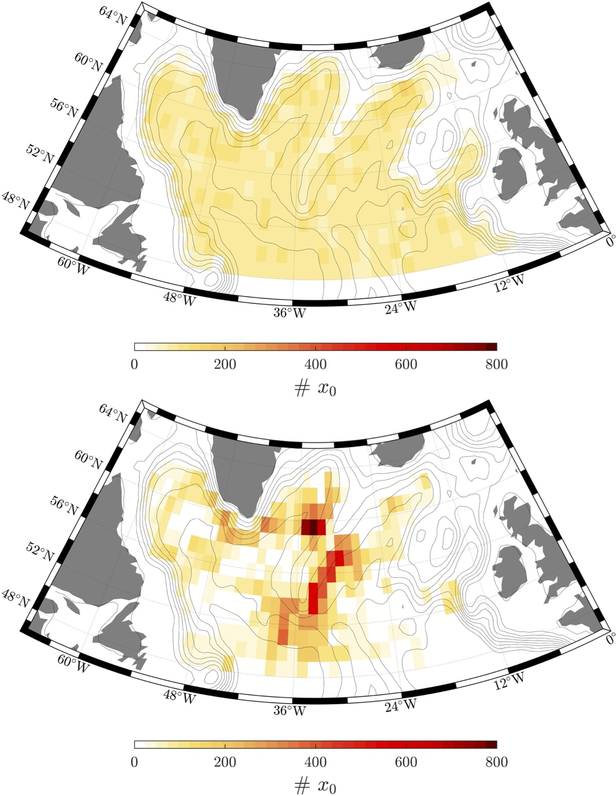
Figure 7: (top panel) Histogram of simulated float initial positions, $x_{0}$, keeping only 7% of them, uniformly at random. The thin gray curves are the isobaths shown in Fig. 1 (bottom panel). As in the top panel, but with $x_{0}$ lying closest to those of the observed float trajectories.

Further support to the need of better sampling for reliable TPT computations is given by studying different realizations of the observed Markov chain constructed with a uniformly at random reduced set of trajectories $(x_{0},x_{T})$. Over these different realizations, we consider the signal-to-noise ratio S/R (mean over standard deviation, also the inverse of the coefficient of variation) as a dimensionless and comparable measure of variability and uncertainty in the data. When S/N is smaller than 1, the standard deviation is larger than the mean, and thus there is large uncertainty and variability in the estimation of the observed chain. In particular, we compute the S/R for each transition probability $P_{ij}$ from box $B_{i}$ to box $B_{j}$ over the different realizations of uniformly at random reduced observed chains. We denote the S/N of each entry $P_{ij}$ by $S_{ij}$. In order to show the resulting ratios on the domain and since the matrix $S$ inherits the sparsity of $P$ and is often zero when $B_{i}$ and $B_{j}$ are not neighbors, we average $S_{ij}$ for each outbound box $B_{i}$ over the set of neighboring boxes. The vector of average ratios is denoted by $\mathbf{s}\in\mathbb{R}^{1\times N}$. The ratio $s_{i}$ of box $B_{i}$ tells us the amount of uncertainty in the estimation of transition probabilities out of box $B_{i}$. A reliable TPT analysis requires a transition matrix $P$ with $\mathbf{s}$ componentwise (sufficiently) greater than 1. The top, middle, and bottom panels of Fig. 8 show estimates of $\mathbf{s}$ for 100 realizations of $P$ obtained by uniformly keeping at random 75, 50, and 25%, respectively, of the available float trajectories. The “noise” consistently masks the “signal” in the majority of the domain. A consistent exception is the eastern flank of the Reykjanes Ridge. This provides reason to distrust the results from the TPT analysis of the observed Markov chain, demanding an improvement of the float data set with more sampling, especially in the western regions where $\mathbf{s}$ is componentwise smaller than $1$.

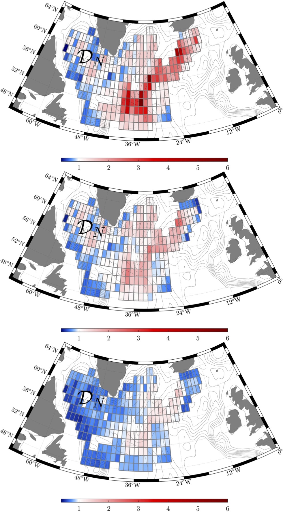
Figure 8: Averaged signal-to-noise ratio of the transition probability between each covering box and neighboring boxes for the observed Markov chain as estimated from 100 realizations thereof constructed using 75 (top panel), 50 (middle panel), and 25 (bottom panel) percent of the available float trajectories, chosen uniformly at random. The thin gray curves are the isobaths shown in Fig. 1.

6 Summary and conclusions

The equatorward export of Iceland–Scotland Overflow Water (ISOW) from the subpolar North Atlantic is a problem that has stirred much debate in recent years. The ISOW is the lighter of the two overflow components of the North Atlantic Deep Water (NADW), which forms the upper limb of Atlantic Meridional Overturning Circulation (AMOC) that flows southward. The AMOC strength and the impacts on the planet’s climate regulation depend on the rates of formation of NADW, and ISOW in particular. Recent analyses of observed deep float trajectories have led investigators to conclude that the traditional abyssal circulation should be revised. Such a theory postulates that ISOW should steadily flow equatorward along a well-organized deep boundary current (DBC) around the subpolar North Atlantic. Unlike those analyses, which involved direct inspection of observed trajectories and the construction of probability distributions from long trajectories integrated using numerically generated velocities, which typically lead to a picture difficult to interpret, here we have applied Transition Path Theory (TPT). TPT is designed to rigorously characterize the ensembles of trajectories that directly connect a source with a target. As such, TPT is very well suited to tackle the ISOW problem as details of individual connecting trajectories are averaged out and instead the average dominant transport channels are found.

TPT was applied on three different time-homogeneous Markov chains on boxes that covered the subpolar North Atlantic, which are useful for framing long-term ISOW motion asymptotics. One was constructed using a high number of simulated trajectories homogeneously covering the flow domain. The other two chains used much fewer trajectories that heterogeneously covered the domain. The trajectories in the latter two chains were observed trajectories or simulated trajectories subsampled at the observed frequency. While the densely sampled chain supported a well-defined DBC, the sparsely sampled chains did not, independent of whether observed or simulated trajectories were involved. By studying the sensitivity of the results to sampling, we conclude that heterogeneous and insufficient sampling might be behind the current debate around the validity of the traditional abyssal circulation theory.

While the required sampling density to unveil, or not, a DBC of ISOW seems beyond the capability of observational platforms at present, the TPT analysis, or any analysis aimed at investigating long-time asymptotics and connectivity, might benefit from a subsurface float dataset enlarged with extra floats deployed in the northern Iceland Basin, where the ISOW enters the subpolar North Atlantic, and in the western flank of the Reykjanes Ridge. The expectation is that trajectories initialized there will reveal any missed communication between the basins west and east of the Reykjanes/Mid-Atlantic Ridge, and also within these basins. The western side, more specifically the Irminger and Labrador Seas, and the Newfoundland Basin, is characterized by transition probabilities with a low signal-to-noise ratio and hence high uncertainty. In turn, the eastern side has a large region, the West European Basin, that is not visited by float trajectories at all. The lack of sampling there attempts against the significance of any transition export paths flanking the Mid-Atlantic Ridge on the east.