30 to 100-kG magnetic fields in the cores of red giant stars

Abstract

A red giant star is an evolved low- or intermediate-mass star that has exhausted its central hydrogen content, leaving a helium core and a hydrogen-burning shell. Oscillations of stars can be observed as periodic dimmings and brightenings in the optical light curves. In red giant stars, non-radial acoustic waves couple to gravity waves and give rise to mixed modes, which behave as pressure (p) modes in the envelope and gravity (g) modes in the core. These modes were previously used to measure the internal rotation of red giants[1, 2], leading to the conclusion that purely hydrodynamical processes of angular momentum transport from the core are too inefficient[3]. Magnetic fields could produce the additional required transport[4, 5, 6]. However, due to the lack of direct measurements of magnetic fields in stellar interiors, very little is currently known about their properties. Asteroseismology can provide direct detection of magnetic fields because, like rotation, the fields induce shifts in the oscillation mode frequencies[7, 8, 9, 10, 11, 12]. Here we report the measurement of magnetic fields in the cores of three red giant stars observed with the Kepler[13] satellite. The fields induce shifts that break the symmetry of dipole mode multiplets. We thus measure field strengths ranging from $\sim$ 30 to $\sim$ 100 kG in the vicinity of the hydrogen-burning shell and place constraints on the field tolopolgy.

Rotation lifts the degeneracy between the angular frequencies $\omega$ of oscillation modes with same degree $l$ and radial order $n$ but different azimuthal order $m$. This produces multiplets with $(2l+1)$ components, which can be used to probe the internal rotation of stars. At first order, rotational multiplets are symmetric with respect to the central ($m=0$) component, as is the case for all red giants studied so far[2]. Magnetic fields are known to break this symmetry [9, 10, 11, 12, 14].

We detected clear asymmetries in the multiplets of three hydrogen-shell burning giants observed with Kepler, namely KIC 8684542, KIC 7518143, and KIC 11515377 (see Fig. 1). We notice several common characteristics for the three stars. First, the asymmetries of dipole multiplets, defined as $\delta_{\rm asym}=\omega_{m=-1}+\omega_{m=+1}-2\omega_{m=0}$[15], consistently have the same sign for each star: they are all positive (or consistent with zero) for KIC 8684542 (Fig. 2) and KIC 7518143, but negative for KIC 11515377. Secondly, the absolute values of the asymmetries are systematically lower for p-dominated modes (dark shaded regions in Fig. 2) than for g-dominated modes (light shaded regions). This indicates that the cause of the asymmetries is located in the core. Finally, the detected asymmetries sharply decrease with frequency.

In the presence of magnetic fields, we showed that, under very general assumptions, the average frequency shift of the components in a dipole multiplet is given by

$$\delta\!\omega_{\rm B}=\frac{\zeta\mathcal{I}}{\mu_{0}\omega^{3}}\int_{r_{\rm i}}^{r_{\rm o}}K(r)\overline{B_{r}^{2}}\,\hbox{d}r,$$ (1)

where $\overline{B_{r}^{2}}$ is a horizontal average of the squared radial field $B_{r}$, $r_{\rm i}$ and $r_{\rm o}$ are the turning points of the g-mode cavity, and $\mathcal{I}$ is a term depending on the core structure[16]. The weight function $K(r)$ sharply peaks near the hydrogen burning shell, so that $\delta\!\omega_{\rm B}$ essentially measures $\overline{B_{r}^{2}}$ near this shell (see Extended Data Fig. 1). The dependence of $\delta\!\omega_{\rm B}$ in $\omega^{-3}$ shows that magnetic perturbations are expected to sharply decrease with frequency. The factor $\zeta$ corresponds to the fraction of the mode kinetic energy that is trapped in the g-mode cavity ($\zeta=1$ for pure gravity modes). Eq. 1 shows that magnetic shifts are expected to be larger for g-dominated modes than for p-dominated modes. The characteristics of magnetic shifts are thus very similar to those of the detected asymmetries.

Asymmetries originate from the dependence of magnetic shifts on $|m|$. The asymmetry of dipole multiplets can be directly related to the average magnetic shift by the expression

$$\delta_{\rm asym}=3a\delta\!\omega_{\rm B}.$$ (2)

The coefficient $a$ involves an average of $B_{r}^{2}$ weighted by the second degree Legendre polynomial $P_{2}(\cos\theta)=(3\cos^{2}\theta-1)/2$, where $\theta$ is the colatitude, and we have shown that $-1/2\leqslant a\leqslant 1$[16]. For instance, a dipole magnetic field ($B_{r}\sim\cos\theta$) yields a positive asymmetry ($a=2/5$). A field that is entirely concentrated on the poles produces maximal asymmetry ($a=1$). Conversely, a field concentrated near the equator gives minimal asymmetry ($a=-1/2$).

We then compared the measured asymmetries to those that would be produced by internal magnetic fields. We fit an expression of $\delta_{\rm asym}$ based on Eq. 1 and 2 to the observed asymmetries. The results are shown in Fig. 2. The agreement with the observed asymmetries is quite good, the overall decrease of the asymmetries with frequency being well reproduced, as well as their modulation with the trapping of the modes in the g- and p-cavities. This confirms that the detected asymmetries are indeed produced by magnetic fields in the cores of these red giants. For completeness, we have also shown that other mechanisms that can produce multiplet asymmetries, such as higher-order rotational effects[17] or near-degeneracy effects[15], cannot account for the observed asymmetries[16].

Eq. 1 can then be used to estimate the squared radial magnetic field $\langle B_{r}^{2}\rangle$ averaged in the horizontal direction, and weighted by the function $K(r)$ in the radial direction, yielding

$$\langle B_{r}^{2}\rangle=\frac{\mu_{0}\delta_{\rm g}\omega_{\rm max}^{3}}{3a\mathcal{I}},$$ (3)

where $\omega_{\mathrm{max}}\equiv 2\pi\nu_{\rm max}$ corresponds to the angular frequency of maximum power of the oscillations and $\delta_{\mathrm{g}}$ is the asymmetry of pure g modes at the frequency of maximum power of the oscillation $\nu_{\rm max}$. The minimal magnetic field that can produce the observed asymmetries is obtained by assuming $a=1$ for stars with positive asymmetries, and $a=-1/2$ for stars with negative asymmetries. To estimate $\mathcal{I}$, we computed models that reproduce the seismic properties of each of the three stars, using the stellar evolution code MESA[18, 16]. We thus obtained minimal magnetic field intensities of 65 kG for KIC 8684542, 26 kG for KIC 7518143, and 70 kG for KIC 11515377.

These fields are expected to produce magnetic shifts in the mode frequencies. We found that magnetic shifts can be detected by their impact on the pattern of pure gravity modes. In the non-magnetic case, the periods of pure g modes with high radial orders $n_{\rm g}$ are given by $P(n_{\rm g})=\Delta\Pi_{1}(n_{\rm g}+\varepsilon_{\rm g})$, where $\Delta\Pi_{1}$ is the asymptotic period spacing. The offset term $\varepsilon_{\rm g}$ is strongly constrained for hydrogen-shell burning giants. From Kepler observations, it was found that $\varepsilon_{\rm g}=0.28\pm 0.08$[19], in agreement with theoretical predictions[20]. We have shown[16] that magnetic shifts are expected to produce an increase in the measured value of $\varepsilon_{\rm g}$.

The two red giants KIC 8684542 and KIC 11515377 have measured values of $\varepsilon_{\rm g}$ that significantly deviate from the expected range ($\varepsilon_{\rm g}=0.50\pm 0.02$ and $0.50\pm 0.03$, respectively). This can be used to directly measure the intensity of magnetic shifts in these stars. For KIC 7518143, the measured $\varepsilon_{\rm g}=0.30\pm 0.03$ is consistent with regular red giants, which can be used to derive an upper limit for the magnetic field intensity.

To retrieve this information, we computed asymptotic expressions of mixed modes including magnetic and rotational perturbations. We optimised the values of the magnetic shift of pure g modes at $\nu_{\rm max}$ ($\delta\!\omega_{\mathrm{g}}$) and the asymmetry coefficient $a$ to reproduce at best the observed mode frequencies. We found an excellent agreement with the observations for the three stars (see Fig. 3). We thus obtained field intensities of $102\pm 12$ kG for KIC 8684542, $98\pm 24$ kG for KIC 11515377, and an upper limit of 41 kG for KIC 7518143. These measurements are fully compatible with the lower limits that were obtained using multiplet asymmetries, which gives further evidence that the oscillation mode perturbations are indeed caused by magnetic fields.

We also obtained measurements of the coefficient $a$ for the three stars, which can be used to place constraints on the geometry of the internal magnetic field. We found $a=0.47\pm 0.12$ for KIC 8684542 and $a=-0.24_{-0.23}^{+0.08}$ for KIC 11515377. These measurements would be consistent with a dipolar field aligned with the rotation axis for the first star ($a=2/5$) and a dipolar field aligned with the equator for the second ($a=-1/5$), although other configurations are naturally possible.

This study provides keys to explore internal magnetic fields along the red giant branch. This type of measurement requires the radial magnetic field to be large enough to produce detectable magnetic splittings, but small enough to remain below a critical value $B_{\rm c}$ above which magnetic tension hampers the propagation of gravity waves[21] (the magnetic fields measured here are indeed below $B_{\rm c}$[16]). The range of field intensities that satisfy both conditions represents about one order of magnitude[16]. Field strengths above $B_{\rm c}$ have been invoked to account for red giants with suppressed dipole modes[21], implying that about 20% of red giants are strongly magnetised[22]. A systematic search for magnetic perturbations in red giants with detected oscillations will give the prevalence of red giants with magnetic fields below $B_{\rm c}$.

The measurement of magnetic fields in the radiative cores of red giants will allow to progress on the origin and evolution of the stellar magnetic field.[23, 24]. The origin of the detected fields could be a convective core dynamo occurring during the main sequence. Our best-fit models indeed indicate that the hydrogen burning shell of the three red giants was convective at the very beginning of the main sequence. The dynamo fields generated at that time may have survived when the core became radiative as they can relax into stable configurations[25] and ohmic diffusion is negligible[26]. Assuming magnetic flux conservation, their strengths should range from 3 to 5 kG to account for the detected fields[16]. This is smaller than the amplitudes predicted by numerical simulations of core convection[27] and dynamo scaling laws[11] by about one order of magnitude, although this could be due to magnetic energy loss during the relaxation process[25] or the post-main sequence evolution[6]. Another possibility is that the detected fields are the remnants of the internal magnetic field of an Ap star. These main sequence intermediate-mass stars possess strong surface oblique dipole[28], whose internal part could have survived the post-main sequence evolution.

Constraints on the field strength and geometry are key to identifying how the redistribution of angular momentum operates inside stars. Our discovery of strong magnetic fields in these red giants first suggests that uniform rotation is enforced in their core up to the hydrogen burning shell. Therefore, the jump in rotation rate between the core and the envelope, which was revealed by asteroseismology[29], must occur at higher radii. Secondly, we show that the Tayler-Spruit dynamo which has been proposed as a possible solution for the angular momentum transport in red giants is not at work in the vicinity of their hydrogen burning shell. Indeed, the predicted amplitude of the radial magnetic field, of the order of 10^-2 G[5], is far too low to account for the 10⁵ G radial fields measured here.

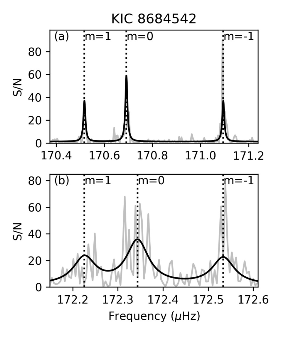
Figure 1: Asymmetric splittings of two mixed modes in KIC 8684542. Panel (a) shows a g-dominated splittings, whereas panel (b) is p-dominated. In each panel, the grey lines show the observed power spectrum and the black lines show the best-fitting model spectrum. The vertical dotted lines mark the locations of the frequencies. Note that the x-axis is re-scaled to align the $m=\pm 1$ modes.

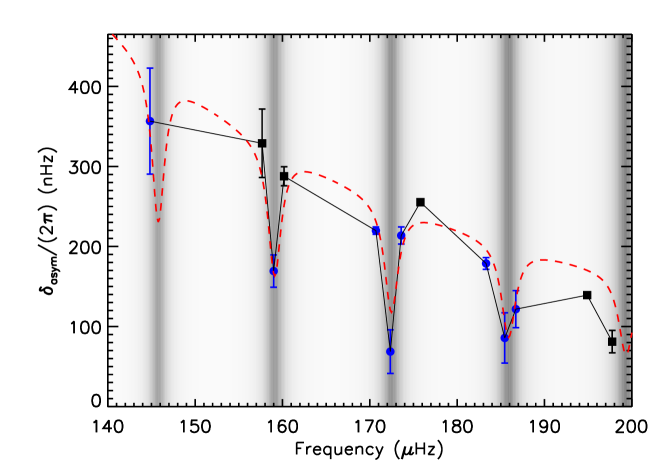
Figure 2: Multiplet asymmetries in KIC 8684542 as a function of mode frequency. Blue circles indicate multiplets with three detected components, and black squares, multiplets with only two. Vertical errorbars indicate 1-$\sigma$ standard deviations. The background shows the $\zeta$ value. Light areas correspond to g-dominated modes and dark ridges show the locations of p-dominated modes. The red dashed curve corresponds to a fit of the theoretical expression of magnetic asymmetries (Eq. 1 and 2) to the observed asymmetries. See also Extended Data Fig. 2 and 3 for KIC 11515377 and KIC 7518143, respectively.

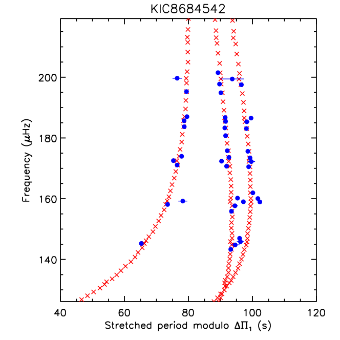
Figure 3: Stretched échelle diagram for KIC 8684542. The periods of dipole mixed modes have been stretched[30] in order to make them regularly spaced in period by the asymptotic period spacing of g modes, $\Delta\Pi_{1}$. Thus, modes with the same azimuthal order $m$ appear nearly vertically aligned in an échelle diagram. Blue circles show the observed frequencies with horizontal errorbars indicating 1-$\sigma$ standard deviations. Red crosses correspond to the best-fit asymptotic mixed mode frequencies obtained by including a magnetic perturbation. See also Extended Data Fig. 4 and 5 for KIC 11515377 and KIC 7518143, respectively.

Data availability

Kepler data are publicly available from the Mikulski Archive for Space Telescopes (MAST) portal at https://archive.stsci.edu. Spectra are available at https://doi.org/10.5281/zenodo.6818371.

Code availability

This study makes use of the stellar evolution code MESA, which is available at https://docs.mesastar.org.

Author contributions statement

G.L. discovered the three stars with asymmetric splittings. G.L. and S.D. measured the asymmetries and rotation rates. S.D. measured the absolute magnetic shifts and supervised the whole project. J.B. and F.L. developed the theoretical framework used to interpret the observations. All the authors contributed to writing the manuscript.

Competing Interest Declaration

The authors declare no competing interests.

Supplementary Information

Supplementary Information is available for this paper.

Author Information

Reprints and permissions information is available at www.nature.com/reprints. Correspondence and requests for materials should be addressed to SD (sebastien.deheuvels@irap.omp.eu).

Extended Data Items

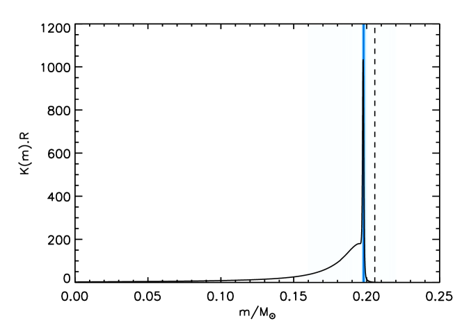
Extended Data Figure 1: Shape of the weight function $K(m)$ as a function of the normalised mass. The function $K(m)$ is shown for the stellar model representative of KIC 11515377. The blue shaded region indicates the hydrogen burning shell. The vertical dashed line corresponds to the maximal extent of the initial convective core at the beginning of the main sequence.

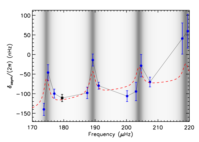
Extended Data Figure 2: Multiplet asymmetries in KIC 11515377 as a function of mode frequency. Symbols have the same meaning as in Figure 2.

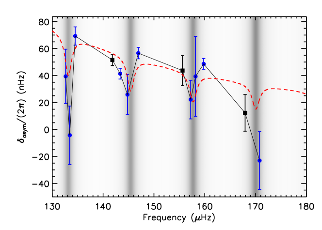
Extended Data Figure 3: Multiplet asymmetries in KIC 7518143 as a function of mode frequency. Symbols have the same meaning as in Figure 2.

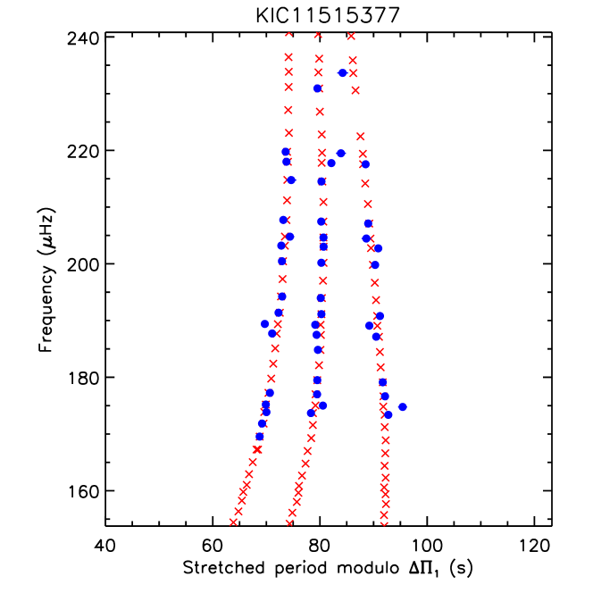
Extended Data Figure 4: Stretched échelle diagram for KIC 11515377. Symbols have the same meaning as in Figure 3.

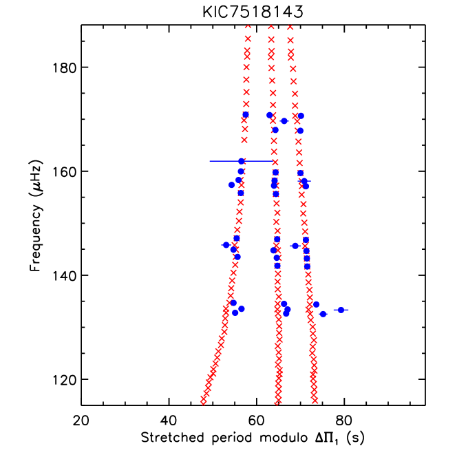
Extended Data Figure 5: Stretched échelle diagram for KIC 7518143. Symbols have the same meaning as in Figure 3.

Supplementary Information

S1 Seismic characterisation and detection of mutliplet asymmetries in three Kepler red giants

We here describe the seismic analysis of the three Kepler red giants KIC 8684542, KIC 11515377, and KIC 7518143, which led us to detect multiplet asymmetries in these stars. Hereafter, ordinary frequencies are denoted as $\nu$. They are related to angular frequencies through $\omega\equiv 2\pi\nu$.

S1.1 Oscillation spectra and global seismic properties

The three stars were selected from the asteroseismic red giant catalogue by Yu et al.[2], which provides the measurements of seismic parameters (such as large separations $\Delta\nu$ and frequencies of maximum power $\nu_{\mathrm{max}}$) and the evolutionary stages (hydrogen-shell burning or core-helium burning) of Kepler red giants with detected oscillations. We downloaded the Kepler long-cadence light curves from the Mikulski Archive for Space Telescopes (MAST, https://archive.stsci.edu), corrected them[3], and calculated the power density spectra (PSD) [4, 5, 6]. Global asteroseismic parameters ($\nu_{\mathrm{max}}$, $\Delta\nu$) and background properties were calculated following the processes used in the SYD pipeline [7, 8].

The radial modes ($l=0$, where $l$ is the angular degree) were identified using an échelle diagram folded with the asymptotic large separation of p modes $\Delta\nu$. The detected peaks were then fit by Lorentzian profiles to estimate the mode parameters (frequencies, linewidths, heights) and their corresponding uncertainties through maximum likelihood estimation[9]. To refine our estimates of p-mode properties, we used a polynomial regression to fit the measured radial mode frequencies to a second-order asymptotic expression of p modes, written as

$$\nu_{l=0}(n)=\left[n+\varepsilon_{\rm p}+\frac{\alpha}{2}(n-n_{\rm max})^{2}\right]\Delta\nu$$ (4)

where $\alpha$ measures the second-order effects in the asymptotic development around $\nu_{\mathrm{max}}$, $\varepsilon_{\rm p}$ is a phase offset, and $n_{\rm max}=\nu_{\rm max}/\Delta\nu$. The results are given in Supplementary Table 1 for the three stars.

S1.2 Identifying dipole mixed modes

Identifying dipole modes in the oscillation spectra is more complicated because these modes show a mixed behaviour and therefore follow neither the asymptotic pattern of p modes, nor the asymptotic pattern of g modes. Representing the oscillation modes in the so-called “stretched” period échelle diagram[30] is particularly helpful to identify the modes. We here only briefly describe this method. It has been shown[30] that the period spacing between consecutive dipole mixed modes can be expressed as $\Delta P=\zeta\Delta\Pi_{1}$, where $\zeta$ is the ratio between the kinetic energy of the mode in the g-mode cavity and the total kinetic energy of the mode ($\zeta$ tends to unity for pure g modes and to zero for pure p modes), and $\Delta\Pi_{1}$ is the asymptotic period spacing of pure g modes. Thus, the so-called “stretched” periods $\tau$, defined by the differential equation $\hbox{d}\tau=\hbox{d}P/\zeta$, are regularly spaced by $\Delta\Pi_{1}$. It is then convenient to show the stretched periods in an échelle diagram folded with $\Delta\Pi_{1}$ because the modes of same azimuthal order $m$ are expected to align nearly vertically in this diagram.

Estimates of $\zeta$ for the detected modes can be obtained from asymptotic relations[10]. Using estimates of $\Delta\Pi_{1}$ from previous studies[2], we were then able to build stretched échelle diagrams for the three red giants under study (Figure 3 and Extended Data Figure 4-5). For each star, three clear ridges are visible, associated with the $m=-1,0,+1$ components of dipole multiplets. It is already visible that the multiplets show significant asymmetries (especially for KIC 8684542), as is further addressed in Sect. S1.3.

In the stretched échelle diagram, the period spacings of modes with the same $m$ value are given by[2]

$$\Delta\tau_{m}=\Delta\Pi_{1}\left(1+mx_{\mathrm{rot}}\right),$$ (5)

with

$$x_{\mathrm{rot}}=2\frac{\mathcal{N}_{\mathrm{max}}}{\mathcal{N}_{\mathrm{max}}+1}\frac{\delta\nu_{\mathrm{R,core}}}{\nu_{\mathrm{max}}},$$ (6)

where $\mathcal{N}_{\mathrm{max}}=\Delta\nu/(\Delta\Pi_{1}\nu_{\mathrm{max}}^{2})$ is the mixed mode density at $\nu_{\mathrm{max}}$, and $\delta\nu_{\mathrm{R,core}}$ is the rotational splitting of pure g modes. Therefore, the identification of the azimuthal order $m$ can be done by comparing the period spacing in the stretched échelle diagram: the larger $m$, the larger $\Delta\tau_{m}$.

S1.3 Detecting multiplet asymmetries

We then extracted the frequencies of the identified dipole modes by fitting Lorentzian profiles to the PSD as described in Sect. S1.1. We note that several codes performing the extraction of oscillation mode properties from the PSD are public[11] and can be used to reproduce our results. We show in Supplementary Figures 1-3 our optimal fits to the PSD for the three stars. The measured mode frequencies are given in Supplementary Table 2. Using the identification from the previous section, we could then compute the asymmetries of the multiplets for which all $m$ components were detected, using the expression

$$\delta_{\rm asym}=\omega_{m=-1}+\omega_{m=+1}-2\omega_{m=0}.$$ (7)

The values of the measured asymmetries are given in Supplementary Tables 3-5. We found very significant asymmetries for all three stars. The measured asymmetries are shown as a function of the mode frequency in Figure 2 and Extended Data Figure 2-3.

S1.4 Refining estimates of g-mode properties

We then used an asymptotic expression of mixed modes[12] to refine our estimates of g-mode properties. For mixed modes, the matching of solutions corresponding to g-modes in the core and to p-modes in the envelope requires that

$$\tan(\theta_{\rm p})=q\tan(\theta_{\rm g}),$$ (8)

where $q$ corresponds to the coupling strength between the two cavities, and $\theta_{\rm p}$, $\theta_{\rm g}$ are phase terms that can be expressed as a function of the asymptotic expressions of p- and g-modes. We have[13]

$$\theta_{\rm p} =\frac{\pi}{\Delta\nu}\left(\nu-\nu_{\rm p}\right),$$ (9)

$$\theta_{\rm g} =\frac{\pi}{\Delta\Pi_{1}}\left(P-P_{\rm g}\right),$$ (10)

where $\nu_{\rm p}$ correspond to the frequencies of $l=1$ pure p modes and $P_{\rm g}$ are the periods of $l=1$ pure g modes. Their asymptotic expressions are given by

$$\nu_{\rm p}(n_{\rm p}) =\nu_{l=0}(n_{\rm p})+\Delta\nu/2-d_{01},$$ (11)

$$P_{\rm g}(n_{\rm g}) =(n_{\rm g}+\varepsilon_{\rm g})\Delta\Pi_{1},$$ (12)

where $d_{01}$ corresponds to the mean small separation built with $l=0$ and 1 pressure modes. Pure g modes are characterised by the asymptotic period spacing $\Delta\Pi_{1}$ and the phase offset $\varepsilon_{\rm g}$.

The parameters $\Delta\nu$, $\alpha$, and $\varepsilon_{\rm p}$ were already measured in Sect. S1.1. For any given set of parameters $(\Delta\Pi_{1},\leavevmode\nobreak\ \varepsilon_{\rm g},\leavevmode\nobreak\ q,\leavevmode\nobreak\ d_{01})$, asymptotic mixed mode frequencies with $m=0$ can be obtained by solving Eq. 8 using the Newton-Raphson algorithm. For each star, we optimised these four parameters to reproduce at best the observed frequencies of $m=0$ dipole modes. For this purpose, we computed grids, exploring wide intervals encompassing reasonable values for the four parameters and we calculated the agreement with the measured frequencies for each grid point. We then computed more refined grids to fine-tune the values of the parameters. The results are given in Supplementary Table 1.

S1.5 Measurement of internal rotation

We then performed a seismic measurement of the internal rotation of the three red giants. Since rotational multiplets are asymmetric in the three stars, the rotational splittings were measured as $\delta\!\omega_{\rm R}=(\omega_{n,m=-1}-\omega_{n,m=+1})/2$ (see Supplementary Tables 3-5). Using asymptotic relations, we have[10]

$$\delta\!\omega_{\rm R}=\frac{\zeta}{2}\langle\Omega\rangle_{\rm g}+(1-\zeta)\langle\Omega\rangle_{\rm p},$$ (13)

where $\langle\Omega\rangle_{\rm g}$ and $\langle\Omega\rangle_{\rm p}$ are the average rotation rates in the g-mode and p-mode cavities, respectively.

The parameter $\zeta$ can be conveniently estimated from the mode frequencies by the relation[10, 14]

$$\zeta=\left[1+q\frac{\nu^{2}\Delta\Pi_{1}}{\Delta\nu}\frac{1}{\sin^{2}\theta_{\rm p}+q^{2}\cos^{2}\theta_{\rm p}}\right]^{-1}.$$ (14)

Using the asymptotic properties of pressure and gravity modes measured in Sect. S1.1 and S1.4, we were able to estimate the value of $\zeta$ for each detected mode.

Supplementary Figure 4 shows the measured rotational splittings as a function of $\zeta$ for the three stars. We recover a linear relation as predicted by Eq. 13. The coefficients of a linear regression of this relation directly provide estimates of the average rotation rates in the g-mode cavity ($\langle\Omega\rangle_{\rm g}$) and in the p-mode cavity ($\langle\Omega\rangle_{\rm p}$). The results are given in Supplementary Table 6. The measurements of $\langle\Omega\rangle_{\rm g}$ for the three stars are in line with the typical core rotation rates of red giants (an average of $\langle\Omega\rangle_{\rm g}/(2\pi)=694$ nHz with a standard deviation of 288 nHz was found for 846 Kepler red giants[2]). The measurements of $\langle\Omega\rangle_{\rm p}$ indicate a slow envelope rotation, in agreement with the expansion of the star as it ascends the red giant branch and in line with the measurements of the average envelope rotation in other red giants[10].

Our measurements of the core and envelope rotation rates can yield estimates of the rotational splitting for all detected multiplets using Eq. 13. Thus, we can derive measurements of the asymmetry for dipole multiplets in which either the $m=-1$ or the $m=+1$ component could not be detected. For instance, if we could measure the frequencies of the $m=0$ and $m=+1$ components, we have

$$\delta_{\rm asym}=2(\omega_{m=1}+\delta\!\omega_{\rm R}-\omega_{m=0}).$$ (15)

This enabled us to obtain a few additional asymmetry measurements for the three stars under study. These data points are shown as black squares in Fig. 2 and Extended Data Fig. 2-3.

S2 Effects of magnetic field: the perturbation method

The effects of magnetic fields on stellar oscillations, treated as a perturbation of the adiabatic oscillations have been studied over the last decades[7, 8]. In recent years, these approaches have been applied to high-order g modes in stars[9], then to mixed modes in red giants considering the simple case of dipolar magnetic fields with different radial profiles, aligned with the rotation axis[10, 11] or possibly inclined[12]. These various works aimed at determining the impact of given magnetic fields on mode frequencies, especially to predict minimal magnetic strengths required to produce detectable asymmetries in red giants for specific field structures[10, 11, 12]. The problem we want to solve here is to deduce properties of stellar magnetic fields from seismic observable quantities. We therefore want to avoid any a priori assumptions on the magnetic field topology and are thus led to develop the perturbation theory for a general magnetic field. This is the purpose of the present section.

S2.1 First-order perturbations

Without magnetic field (or rotation), the equations of oscillations in a spherical star reduce to the eigenvalue problem[7]

$${\cal L}_{0}(\bm{\xi})=\omega^{2}\bm{\xi},$$ (16)

where the operator ${\cal L}_{0}(\bm{\xi})\equiv\rho^{-1}\bm{\nabla}p^{\prime}+\bm{\nabla}\psi^{\prime}+\rho^{-1}\bm{\nabla}\psi\rho^{\prime}$ is a linear functional of the displacement $\bm{\xi}$. The quantities $\rho$ and $\psi$ are the equilibrium density and gravitational potential, $p^{\prime}$, $\rho^{\prime}$ and $\psi^{\prime}$ the perturbations to pressure, density and gravitational potential.

In the presence of a magnetic field, the Lorentz force must be taken into account. The problem becomes[8]

$$[{\cal L}_{0}+{\cal L}_{\mathrm{L}}](\bm{\xi})=\omega^{2}\bm{\xi},$$ (17)

with

$${\cal L}_{\mathrm{L}}(\bm{\xi})=-\frac{1}{\rho\mu_{0}}[(\bm{\nabla}\times\bm{B}^{\prime})\times\bm{B}+(\bm{\nabla}\times\bm{B})\times\bm{B}^{\prime}]-\frac{\bm{\nabla}\cdot(\rho\bm{\xi})}{\rho^{2}\mu_{0}}[(\bm{\nabla}\times\bm{B})\times\bm{B}],$$ (18)

where $\bm{B}$ is the magnetic field, $\bm{B}^{\prime}=\bm{\nabla}\times(\bm{\xi}\times\bm{B})$ is the Eulerian perturbation to $\bm{B}$, and $\mu_{0}$ is the magnetic permeability.

We assume that the perturbation introduced by the Lorentz force is small (${\cal L}_{\mathrm{L}}(\bm{\xi})\equiv{\cal L}_{1}(\bm{\xi})$, $\|{\cal L}_{1}(\bm{\xi})\|\ll\|{\cal L}_{0}(\bm{\xi})\|$), and we thus perform a first-order perturbation analysis[7, 8].

Let us denote as $\bm{\xi}_{m}^{(0)}=\xi_{r}(r)Y_{l}^{m}\bm{e}_{r}+\xi_{h}(r)r\bm{\nabla}Y_{l}^{m}$ the eigenfunction of ${\cal L}_{0}$ associated with the eigenfrequency $\omega^{(0)}$ for a given $m$. Spherical harmonics are denoted as $Y_{l}^{m}$ and are normalised such that $\iint Y_{l}^{m}\sin\theta\,\mathrm{d}\theta\,\mathrm{d}\phi=1$, and ($\bm{e}_{r}$, $\bm{e}_{\theta}$, $\bm{e}_{\phi}$) is the usual spherical base. The functions $\xi_{r}$ and $\xi_{h}$ are independent of $m$.

Due to the degeneracy with $m$, any linear combination

$$\bm{\xi}^{(0)}=\sum_{m^{\prime}=-l}^{l}a_{m^{\prime}}\bm{\xi}_{m^{\prime}}^{(0)}$$ (19)

is an eigenfunction of ${\cal L}_{0}$ associated with $\omega^{(0)}$.

The eigenvalues and eigenvectors of the perturbed operator ${\cal L}_{0}+{\cal L}_{1}$ are written as perturbations of the unperturbed solutions: $\omega=\omega^{(0)}+\omega^{(1)}$ and $\bm{\xi}=\bm{\xi}^{(0)}+\bm{\xi}^{(1)}$, with $\omega^{(1)}\ll\omega^{(0)}$ and $\|\bm{\xi}^{(1)}\|\ll\|\bm{\xi}^{(0)}\|$.

The problem reads

$$\left(\omega^{(0)}+\omega^{(1)}\right)^{2}\left(\bm{\xi}^{(0)}+\bm{\xi}^{(1)}\right)=[{\cal L}_{0}+{\cal L}_{1}]\left(\bm{\xi}^{(0)}+\bm{\xi}^{(1)}\right).$$ (20)

We expand this equation and project it on $\bm{\xi}_{m}^{(0)}$. By keeping first-order terms only, it reads

$$2\omega^{(0)}\omega^{(1)}\left\langle\bm{\xi}_{m}^{(0)},\bm{\xi}^{(0)}\right\rangle=\left\langle\bm{\xi}_{m}^{(0)},{\cal L}_{1}\left(\bm{\xi}^{(0)}\right)\right\rangle\quad\forall m$$ (21)

where we have defined the usual inner product

$$\left\langle\bm{f},\bm{g}\right\rangle=\iiint\bm{f}^{*}\cdot\bm{g}\ \rho r^{2}\sin\theta\,\mathrm{d}r\,\mathrm{d}\theta\,\mathrm{d}\phi,$$ (22)

and taken advantage of the Hermitian character of the operator ${\cal L}_{0}$ [15]. By using Eq. 19 and after some algebra, we obtain

$$2\omega^{(0)}\omega^{(1)}a_{m}\left\langle\bm{\xi}_{m}^{(0)},\bm{\xi}_{m}^{(0)}\right\rangle=\sum_{m^{\prime}=-l}^{l}a_{m^{\prime}}\left\langle\bm{\xi}_{m}^{(0)},{\cal L}_{1}\left(\bm{\xi}^{(0)}_{m^{\prime}}\right)\right\rangle\quad\forall m.$$ (23)

Since the operator ${\cal L}_{1}$ is not axisymmetric, the equations for different $m$ are coupled and must be solved simultaneously. We thus face an algebraic eigenvalue problem[12]:

$$\omega^{(1)}\mathsf{a}=\mathsf{Ma},$$ (24)

where the components of eigenvectors $\mathsf{a}$ are the coefficients $a_{m^{\prime}}$, and the elements of the matrix $\mathsf{M}$ are

$$\mathsf{M}_{m,m^{\prime}}=\frac{\left\langle\bm{\xi}_{m}^{(0)},{\cal L}_{\mathrm{L}}\left(\bm{\xi}^{(0)}_{m^{\prime}}\right)\right\rangle}{2\omega^{(0)}\left\langle\bm{\xi}_{m}^{(0)},\bm{\xi}_{m}^{(0)}\right\rangle}.$$ (25)

We recognise in the denominator the mode inertia

$$\left\langle\bm{\xi}_{m}^{(0)},\bm{\xi}_{m}^{(0)}\right\rangle=\int(|\xi_{r}|^{2}+l(l+1)|\xi_{h}|^{2})\rho r^{2}\,\mathrm{d}r\equiv{I},$$ (26)

which does not depend on $m$.

S2.2 Application to high-order g modes

To go further, we make some simplifying assumptions [9]. We consider from now on high-order pure g modes, that is, short radial wavelengths such that $k_{r}/k_{h}\sim N/\omega\gg 1$, where $k_{r}$ and $k_{h}$ are the radial and horizontal components of the wave vector and $N$ denotes the Brunt-Väisälä frequency. As $\xi_{h}/\xi_{r}\sim k_{r}/k_{h}$, this implies that $\xi_{r}\ll\xi_{h}$ and that the radial derivatives of $\xi_{h}$ and $\xi_{r}$ are dominant terms (e.g. $r\partial_{r}\xi_{h}\sim rk_{r}\xi_{h}\gg\xi_{h}$). Moreover, the magnetic field is supposed to vary over large scales $L$, such that $Lk_{r}\gg 1$, and the anisotropy between its components is also limited, that is, $B_{\phi}/B_{r}\ll k_{r}/k_{h}\sim N/\omega$. In the three studied red giant stars the ratio $N/\omega$ is worth $\sim 10^{2}$.

Under these assumptions, we simplify ${\cal L}_{\mathrm{L}}$ (Eq. 18). Since we consider g modes, the last term related to compressibility may be neglected, and among the two others only the first term is dominant[9, 10, 11, 12], thus

$${\cal L}_{\mathrm{L}}(\bm{\xi})\approx-\frac{1}{\rho\mu_{0}}[(\bm{\nabla}\times\bm{B}^{\prime})\times\bm{B}].$$ (27)

Using this simplified expression, we show after some algebra that

$$\left\langle\bm{\xi}_{m}^{(0)},{\cal L}_{\mathrm{L}}\left(\bm{\xi}^{(0)}_{m^{\prime}}\right)\right\rangle=\frac{1}{\mu_{0}}\iiint{{\bm{B}^{\prime}}_{m}^{(0)}}^{\mbox{*}}\cdot{\bm{B}^{\prime}}_{m^{\prime}}^{(0)}\,r^{2}\sin\theta\,\mathrm{d}r\,\mathrm{d}\theta\,\mathrm{d}\phi,$$ (28)

where ${\bm{B}^{\prime}}_{m}^{(0)}=\bm{\nabla}\times(\bm{\xi}_{m}^{(0)}\times\bm{B})$. We recover the expression obtained for axisymmetric fields[9, 10, 11] when $m^{\prime}=m$. To obtain this expression, we neglected a surface term by assuming that it is negligible with respect to the volume integral term. This is relevant in particular when the field decays towards the outer part of the g-mode cavity[12]. The Eulerian perturbation to the field simplifies to

$${\bm{B}^{\prime}}_{m}^{(0)}=\dfrac{\partial(r\xi_{h})}{\partial r}B_{r}\bm{\nabla}Y_{l}^{m}.$$ (29)

Thus we get

$$\left\langle\bm{\xi}_{m}^{(0)},{\cal L}_{\mathrm{L}}\left(\bm{\xi}^{(0)}_{m^{\prime}}\right)\right\rangle=\\ \frac{1}{\mu_{0}}\int_{r_{\rm i}}^{r_{\rm o}}\left[\frac{\partial(r\xi_{h})}{\partial r}\right]^{2}\int_{0}^{2\pi}\!\!\int_{0}^{\pi}B_{r}^{2}e^{i(m^{\prime}-m)\phi}\left[\frac{\partial{\hat{Y}_{l}^{m}}}{\partial\theta}\frac{\partial{\hat{Y}_{l}^{m^{\prime}}}}{\partial\theta}+\frac{mm^{\prime}}{\sin^{2}\theta}\hat{Y}_{l}^{m}\hat{Y}_{l}^{m^{\prime}}\right]\sin\theta\,\mathrm{d}\theta\,\mathrm{d}\phi\,\mathrm{d}r,$$ (30)

where $r_{\rm i}$ and $r_{\rm o}$ are the inner and outer boundaries of the g-mode cavity, and $\hat{Y}_{l}^{m}(\theta)$ is defined as $Y_{l}^{m}(\theta,\phi)=\hat{Y}_{l}^{m}(\theta)e^{im\phi}$. We notice that, in the limit of short radial wavelengths, g-mode frequencies are only sensitive to the square of the radial component of the magnetic field.

Finally, the inertia (Eq. 26) of high-order g modes is

$${I}\approx l(l+1)\int_{r_{\rm i}}^{r_{\rm o}}|\xi_{h}|^{2}\rho r^{2}\,\mathrm{d}r.$$ (31)

S2.3 Effects of magnetic field on high-order dipole g modes

For clarity we drop in the following sections the superscript “$(0)$” in $\omega^{(0)}$. Using Eqs. 30 and 31, the matrix elements $\mathsf{M}_{m,m^{\prime}}$ (Eq. 25) for $l=1$ high-order g modes read

$$\mathsf{M}_{1,1}=\mathsf{M}_{-1,-1} = \frac{1}{2\mu_{0}\omega{I}}\frac{3}{4}\int_{r_{\rm i}}^{r_{\rm o}}[\partial_{r}(r\xi_{h})]^{2}\int_{0}^{\pi}\left[B_{r}^{2}\right]_{0}(1+\cos^{2}\theta)\sin\theta\,\mathrm{d}\theta\,\mathrm{d}r,$$ (32)

$$\mathsf{M}_{0,0} = \frac{1}{2\mu_{0}\omega{I}}\frac{3}{2}\int_{r_{\rm i}}^{r_{\rm o}}[\partial_{r}(r\xi_{h})]^{2}\int_{0}^{\pi}\left[B_{r}^{2}\right]_{0}(1-\cos^{2}\theta)\sin\theta\,\mathrm{d}\theta\,\mathrm{d}r,$$ (33)

$$\mathsf{M}_{0,1}=-\mathsf{M}_{-1,0} = \frac{1}{2\mu_{0}\omega{I}}\frac{3}{2\sqrt{2}}\int_{r_{\rm i}}^{r_{\rm o}}[\partial_{r}(r\xi_{h})]^{2}\int_{0}^{\pi}\left[B_{r}^{2}\right]_{1}(\sin\theta\cos\theta)\sin\theta\,\mathrm{d}\theta\,\mathrm{d}r,$$ (34)

$$\mathsf{M}_{1,0}=-\mathsf{M}_{0,-1} = \mathsf{M}_{0,1}^{*},$$ (35)

$$\mathsf{M}_{-1,1}=\mathsf{M}_{1,-1}^{*} = \frac{1}{2\mu_{0}\omega{I}}\frac{3}{4}\int_{r_{\rm i}}^{r_{\rm o}}[\partial_{r}(r\xi_{h})]^{2}\int_{0}^{\pi}\left[B_{r}^{2}\right]_{2}(1-\cos^{2}\theta)\sin\theta\,\mathrm{d}\theta\,\mathrm{d}r,$$ (36)

where $\left[B_{r}^{2}\right]_{k}$ are the Fourier coefficients along $\phi$ of $B_{r}^{2}$ defined as

$$\left[B_{r}^{2}\right]_{k}(r,\theta)=\frac{1}{2\pi}\int_{0}^{2\pi}B_{r}^{2}e^{ik\phi}\,\mathrm{d}\phi.$$ (37)

The matrix $\mathsf{M}$ is Hermitian and thus its eigenvalues are real. We detail hereafter some properties of matrix $\mathsf{M}$ that are useful to exploit the observed spectra.

Trace

The trace of $\mathsf{M}$, $\mathrm{Tr}(\mathsf{M})$, is also the sum of its eigenvalues, i.e. $\omega_{m=-1}^{(1)}+\omega_{m=0}^{(1)}+\omega_{m=+1}^{(1)}$. It reads

$$\mathrm{Tr}(\mathsf{M})=3\omega_{\mathrm{B}}\quad\mbox{with}\quad\omega_{\mathrm{B}}=\frac{1}{2\mu_{0}\omega I}\int_{r_{\rm i}}^{r_{\rm o}}[\partial_{r}(r\xi_{h})]^{2}\int_{0}^{\pi}\left[B_{r}^{2}\right]_{0}\sin\theta\,\mathrm{d}\theta\,\mathrm{d}r.$$ (38)

Let us define the horizontal average of the squared radial magnetic field as

$$\overline{B_{r}^{2}}=\frac{1}{4\pi}\iint B_{r}^{2}\sin\theta\,\mathrm{d}\theta\,\mathrm{d}\phi,$$ (39)

then

$$\omega_{\mathrm{B}}=\frac{1}{2\mu_{0}\omega}\frac{\displaystyle\int_{r_{\rm i}}^{r_{\rm o}}[\partial_{r}(r\xi_{h})]^{2}\overline{B_{r}^{2}}\,\mathrm{d}r}{\displaystyle\int_{r_{\rm i}}^{r_{\rm o}}\xi_{h}^{2}\rho r^{2}\,\mathrm{d}r}.$$ (40)

We use the asymptotic expression of the displacement for high-order g modes[7]

$$\xi_{h}\sim\rho^{-1/2}r^{-3/2}N^{1/2}\sin\left[\Phi(r)\right]$$ (41)

with the phase $\displaystyle\Phi(r)=\int_{r_{\rm i}}^{r}k_{r}(r^{\prime})\,\mathrm{d}r^{\prime}-\frac{\pi}{4}$. Thus Eq. 40 reduces to:

$$\omega_{\mathrm{B}}=\frac{1}{\mu_{0}\omega^{3}}\frac{\displaystyle\int_{r_{\rm i}}^{r_{\rm o}}\left(\frac{N}{r}\right)^{3}\frac{\overline{B_{r}^{2}}}{\rho}\,\mathrm{d}r}{\displaystyle\int_{r_{\rm i}}^{r_{\rm o}}\frac{N}{r}\,\mathrm{d}r}.$$ (42)

We have used the Stationary Phase Approximation, which is valid for rapidly oscillating functions such as $\Phi(r)$, to take out the phase terms[14]. This expression we found here to characterise the trace is similar to the equations describing magnetic shifts for axisymmetric fields[26, 14]. We can rewrite $\omega_{\mathrm{B}}$ as

$$\omega_{\mathrm{B}}=\frac{\mathcal{I}}{\mu_{0}\omega^{3}}\int_{r_{\rm i}}^{r_{\rm o}}K(r)\overline{B_{r}^{2}}\,\hbox{d}r\equiv\frac{\mathcal{I}}{\mu_{0}\omega^{3}}\langle B_{r}^{2}\rangle,$$ (43)

where $K(r)$ is a weight function

$$K(r)=\frac{\displaystyle\frac{1}{\rho}\left(\frac{N}{r}\right)^{3}}{\displaystyle\int_{r_{\rm i}}^{r_{\rm o}}\left(\frac{N}{r}\right)^{3}\frac{\hbox{d}r}{\rho}},$$ (44)

and $\cal I$ is a factor depending on the core structure

$$\mathcal{I}=\frac{\displaystyle\int_{r_{\rm i}}^{r_{\rm o}}\left(\frac{N}{r}\right)^{3}\frac{\hbox{d}r}{\rho}}{\displaystyle\int_{r_{\rm i}}^{r_{\rm o}}\left(\frac{N}{r}\right)\,\hbox{d}r}.$$ (45)

Magnetic effects thus vary as $1/\omega^{3}$. This dependency, which was found for dipole fields[9, 10, 11, 12], is generalised here. A typical profile of the function $K$ in red giant stars is plotted in Extended Data Figure 1. Compared to rotation kernels, the function $K$ peaks in a very narrow range located at the hydrogen burning shell due to the cubic dependency of $N/r$.

Range for the matrix elements

Using inequality relations between integrals, and noticing that $|x\sqrt{1-x^{2}}|\leqslant(1+x^{2})/(2\sqrt{2})$ over $[-1,1]$, we show that

$$\frac{3}{4}\omega_{\mathrm{B}}\leqslant\mathsf{M}_{11}\leqslant\frac{3}{2}\omega_{\mathrm{B}},\quad 0\leqslant\mathsf{M}_{00}\leqslant\frac{3}{2}\omega_{\mathrm{B}},\quad|\mathsf{M}_{01}|\leqslant\frac{1}{2}\mathsf{M}_{11}\quad{\mbox{and}}\quad|\mathsf{M}_{-11}|\leqslant\frac{1}{2}\mathsf{M}_{00}.$$ (46)

Asymmetry

As shown in Sect. S2.7, the asymmetry of multiplets $\delta_{\mathrm{asym}}$ corresponds in many cases to the quantity $2(\mathsf{M}_{11}-\mathsf{M}_{00})$. Using Eqs. 32 and 33, it reads

$$2(\mathsf{M}_{11}-\mathsf{M}_{00})=\frac{3}{4\mu_{0}\omega I}\int_{r_{\rm i}}^{r_{\rm o}}[\partial_{r}(r\xi_{h})]^{2}\int_{0}^{\pi}\left[B_{r}^{2}\right]_{0}(3\cos^{2}\theta-1)\sin\theta\,\hbox{d}\theta\,\hbox{d}r$$ (47)

We recognise an average of $B_{r}^{2}$ weighted with the second degree Legendre polynomial $P_{2}(\cos\theta)=(3\cos^{2}\theta-1)/2$. We can rewrite this equation as

$$2(\mathsf{M}_{11}-\mathsf{M}_{00})=3a\omega_{\mathrm{B}}$$ (48)

with the asymmetry parameter $a$ defined as

$$a=\frac{\displaystyle\int_{r_{\rm i}}^{r_{\rm o}}K(r)\iint B_{r}^{2}P_{2}(\cos\theta)\sin\theta\,\hbox{d}\theta\hbox{d}\phi\,\hbox{d}r}{\displaystyle\int_{r_{\rm i}}^{r_{\rm o}}K(r)\iint B_{r}^{2}\sin\theta\,\hbox{d}\theta\hbox{d}\phi\,\hbox{d}r}.$$ (49)

This quantity is a measure of the asymmetry of the azimuthal average of $B_{r}^{2}$ between the poles and the equator, averaged over the resonant cavity with the weight function $K$. Since $-1/2\leqslant P_{2}(\cos\theta)\leqslant 1$, we deduce that the possible range for $a$ is limited to

$$-\frac{1}{2}\leqslant a\leqslant 1.$$ (50)

Extreme values for $a$ are reached when $B_{r}^{2}$ is totally concentrated around the poles ($a=1$) or when it is concentrated along the equator ($a=-1/2$). When $B_{r}$ has an axisymmetric dipolar structure ($B_{r}\propto\cos\theta$), we recover $a=2/5$ as already known[9]. For an inclined dipole, $a$ decreases as the inclination increases. It vanishes for an inclination of $\sim 55^{\circ}$, then becomes negative and reaches $a=-1/5$ when the dipole is aligned with the equator.

S2.4 Effects of magnetic field on mixed modes

Thus far we have described the perturbations induced on the frequencies of pure g modes. The non-radial modes observed in red giants are mixed modes. The magnetic shift of p modes being proportional to the square of the ratio of the Alfvén velocity to the sound speed in the convective envelope[14], it is expected to be negligible. Therefore, we assume that the magnetic field only affects the g-mode cavity. For mixed modes, the matrix is then simply

$$\mathsf{M}^{\mathrm{(mixed)}}=\zeta\mathsf{M}$$ (51)

where $\zeta$ is the ratio between the kinetic energy of the mode in the g-mode cavity and the total kinetic energy of the mode. This result for magnetic fields is derived with the same approach as for rotation[10].

S2.5 Combined effects of rotation and magnetic field on mixed modes

Let us consider a star, with a magnetic field, spinning with the rotation profile $\Omega(r)$. We denote as $\langle\Omega\rangle_{\rm g}$ and $\langle\Omega\rangle_{\rm p}$ the average rotation rates in the g-mode and p-mode cavities, respectively. Let us assume that, in the frame rotating with a rotation rate $\langle\Omega\rangle_{\rm g}$, the magnetic field is steady. In this frame, the rotation profile is $\Omega(r)-\langle\Omega\rangle_{\rm g}$. The first-order perturbations $\omega^{(1)}$ of the frequency $\omega^{(0)}$ of a dipole mixed mode in the rotating frame are calculated by solving

$$\omega^{(1)}\mathsf{a}=(\zeta\mathsf{M}+\mathsf{R})\mathsf{a}.$$ (52)

The first term comes from Eq. 51, and the matrix $\mathsf{R}$ combines the effects of the Coriolis force and of the residual azimuthal flow in the rotating frame. It is a diagonal matrix with elements

$$\mathsf{R}_{m,m}=m\omega_{\mathrm{R}},$$ (53)

where

$$\omega_{\mathrm{R}}=\left(1-\frac{\zeta}{2}\right)\langle\Omega\rangle_{\rm g}-(1-\zeta)\langle\Omega\rangle_{\rm p}.$$ (54)

By defining $b=\zeta\omega_{\mathrm{B}}/\omega_{\mathrm{R}}$, a parameter characterising the effects of the magnetic field relative to those of rotation, we can rewrite the matrix $\zeta\mathsf{M}+\mathsf{R}$ as

$$\zeta\mathsf{M}+\mathsf{R}=\omega_{\mathrm{R}}\begin{bmatrix}b\left(1+\dfrac{a}{2}\right)-1&-bc&bd\\ -bc^{*}&b(1-a)&bc\\ bd^{*}&bc^{*}&b\left(1+\dfrac{a}{2}\right)+1\end{bmatrix},$$ (55)

where $a$ is the asymmetry parameter (Eq. 49), and $c$ and $d$ parameterise the off-diagonal elements generated by non-axisymmetric components of $B_{r}^{2}$. Possible values for $c$ and $d$ are constrained by Eq. 46: $|c|\leqslant 1/2+a/4$ and $|d|\leqslant(1-a)/2$.

By solving Eq. 52, we find three frequencies $\omega_{m}=\omega^{(0)}+\omega_{m}^{(1)}$ ($m=-1,0,1$) in the rotating frame, associated with three vectors $\mathsf{a}_{m}$ describing the decomposition of the eigenfunctions on $\bm{\xi}_{m^{\prime}}^{(0)}$ (see Eq. 19). In the inertial frame, we obtain up to nine frequencies[8, 12]

$$\omega_{m,m^{\prime}}=\omega_{m}-m^{\prime}\langle\Omega\rangle_{\rm g},$$ (56)

each frequency being related to the amplitude $\mathsf{a}_{m,m^{\prime}}$ ($\equiv$ $m^{\prime}$-th component of vector $\mathsf{a}_{m}$). When $\mathsf{M}$ is diagonal, only $\omega_{m,m}=\omega_{m}-m\langle\Omega\rangle_{\rm g}$ are associated with non-zero amplitudes.

S2.6 Average shift of multiplets

In the very general case, a $l=1$ multiplet has nine components. We introduce the frequency shift of a mode relative to its unperturbed frequency: $\delta\!\omega_{m,m^{\prime}}=\omega_{m,m^{\prime}}-\omega^{(0)}$. The average of the frequency shifts of the nine components of a multiplet, denoted as $\delta\!\omega_{\mathrm{B}}$, is

$$\delta\!\omega_{\mathrm{B}}=\frac{1}{9}\sum_{m,m^{\prime}}\delta\!\omega_{m,m^{\prime}}=\frac{1}{9}\sum_{m,m^{\prime}}\omega_{m}^{(1)}-m^{\prime}\langle\Omega\rangle_{\rm g}.$$ (57)

Since the trace of a matrix is the sum of its eigenvalues,

$$\omega_{m=+1}^{(1)}+\omega_{m=0}^{(1)}+\omega_{m=-1}^{(1)}=\mathrm{Tr}(\zeta\mathsf{M+R})=\zeta\mathrm{Tr}(\mathsf{M})=3\zeta\omega_{\mathrm{B}},$$ (58)

by using $\mathrm{Tr}(\mathsf{R})=0$ and Eq. 38. We deduce that the average frequency shift is

$$\delta\!\omega_{\mathrm{B}}=\zeta\omega_{\mathrm{B}}.$$ (59)

In several practical cases, only $m=m^{\prime}$ components are visible. To simplify the notations, we write $\delta\!\omega_{m}\equiv\delta\!\omega_{m,m}$. Thereby, even when only triplets are visible, we still verify

$$\delta\!\omega_{\mathrm{B}}=\frac{1}{3}(\delta\!\omega_{m=+1}+\delta\!\omega_{m=0}+\delta\!\omega_{m=-1})=\zeta\omega_{\mathrm{B}}.$$ (60)

Thus, measuring the average shift $\delta\!\omega_{\mathrm{B}}$ of a multiplet provides a direct measurement of $\zeta\omega_{\mathrm{B}}$. We also show that $\omega_{\mathrm{B}}$  represents the average magnetic shift of pure g modes.

S2.7 Splitting and asymmetry of triplets

Simple analytic expressions of mode frequencies are possible in two cases: (i) when the diagonal elements of the matrix $\zeta\mathsf{M}+\mathsf{R}$ dominate over the other ones; (ii) when $c$ vanishes.

Diagonally dominated matrix

Case (i) is achieved either for small values of $b$, that is, when the rotational effects dominate over the magnetic ones, or for small values of $|c|$ and $|d|$, which occurs for example when $B_{r}^{2}$ is largely axisymmetric. Nevertheless a field does not need to be axisymmetric to nullify $c$ and $d$, it is sufficient that the Fourier coefficients $\left[B_{r}^{2}\right]_{1}$ and $\left[B_{r}^{2}\right]_{2}$ vanish. The frequency shifts are then:

$$\delta\!\omega_{m=0} = \zeta(1-a)\omega_{\mathrm{B}},$$ (61)

$$\delta\!\omega_{m=\pm 1} = \zeta(1+a/2)\omega_{\mathrm{B}}\pm(\omega_{\mathrm{R}}-\langle\Omega\rangle_{\rm g}).$$ (62)

We deduce that the splitting, defined as $\delta\!\omega_{\mathrm{R}}=\frac{1}{2}(\omega_{m=-1}-\omega_{m=+1})$, is

$$\delta\!\omega_{\mathrm{R}}=\langle\Omega\rangle_{\rm g}-\omega_{\mathrm{R}}=\frac{\zeta}{2}\langle\Omega\rangle_{\rm g}+(1-\zeta)\langle\Omega\rangle_{\rm p}.$$ (63)

In this configuration, the splitting depends only on the rotation, and we recover the same expression as for the non-magnetic case[10].

The asymmetry of a triplet, defined as $\delta_{\mathrm{asym}}=\omega_{m=-1}+\omega_{m=+1}-2\omega_{m=0}$, is

$$\delta_{\mathrm{asym}}=3a\zeta\omega_{\mathrm{B}}=3a\delta\!\omega_{\mathrm{B}}.$$ (64)

The asymmetry is proportional to $\omega_{\mathrm{B}}$, hence to $\langle B_{r}^{2}\rangle$, but also directly depends on the asymmetry parameter $a$ that we have introduced in Eq. 49. As a consequence, when $a=0$, $\delta_{\mathrm{asym}}$ also vanishes, even if the magnetic field is not weak: a weak asymmetry does not necessarily mean a weak magnetic field. This relation shows that $\delta_{\mathrm{asym}}$ can be negative, as we observed in one of our three targets. Without any hypothesis on the magnetic field topology, the asymmetry $\delta_{\mathrm{asym}}$ provides a lower limit of $\langle B_{r}^{2}\rangle$. Measuring simultaneously asymmetries $\delta_{\mathrm{asym}}$ and global shifts $\delta\!\omega_{\mathrm{B}}$ provides a measurement of the rms radial magnetic field as well as a measurement of $a$, that is, information on the latitudinal variations of $B_{r}^{2}$.

Non-axisymmetric effects

In case (ii), $c=0$, we find five components with non-null amplitudes. However, we find that in each vector $\mathsf{a}_{m}$, the component $\mathsf{a}_{m,m}$ are always the largest. As a consequence, among possible components, three of them always have dominant amplitudes: $\omega_{m,m}$ ($m=-1,0,+1$). The frequency shifts for these three components are

$$\delta\!\omega_{m=0} = \zeta(1-a)\omega_{\mathrm{B}},$$ (65)

$$\delta\!\omega_{m=\pm 1} = \zeta(1+a/2)\omega_{\mathrm{B}}\pm\left(\alpha\omega_{\mathrm{R}}-\langle\Omega\rangle_{\rm g}\right).$$ (66)

with $\alpha=\sqrt{1+|bd|^{2}}$. We recover the previous case for $\alpha=1$. We notice that the asymmetry remains unchanged ($\delta_{\mathrm{asym}}=3a\zeta\omega_{\mathrm{B}}$) independently of the value of $\alpha$. However the splitting is affected by the magnetic field in this configuration:

$$\delta\!\omega_{\mathrm{R}}=\langle\Omega\rangle_{\rm g}-\alpha\omega_{\mathrm{R}}=(1-\alpha-\alpha\zeta/2)\langle\Omega\rangle_{\rm g}+\alpha(1-\zeta)\langle\Omega\rangle_{\rm p}.$$ (67)

Since $\alpha$ depends on $\omega_{\mathrm{B}}$, which varies as $1/\omega^{3}$, $\delta\!\omega_{\mathrm{R}}$ is not a simple linear function of $\zeta$. The non-axisymmetric terms introduce a spread in this linear relation. As a consequence, when we observe a tight linear relation between $\delta\!\omega_{\mathrm{R}}$ and $\zeta$, the quasi-axisymmetric approach should be valid.

Having non-null $c$ makes the situation more complex. When $|bc|$ becomes large, the expression for the asymmetry is more complicated. However, a parametric study shows us that, as long as $b<1$, only the three components $\mathsf{a}_{m,m}$ are non-negligible. For higher values of $b$, the number of high-amplitude components changes and depends on the values of $c$ and $d$, making the spectrum more difficult to interpret. The reward of a successful spectrum interpretation would be to provide information on the non-axisymmetric components of $B_{r}^{2}$, $\left[B_{r}^{2}\right]_{1}$ and $\left[B_{r}^{2}\right]_{2}$, in addition to $a$ and $\omega_{\mathrm{B}}$.

For test purposes, we applied our expressions to inclined dipolar fields, which have already been studied[12]. The splittings and asymmetries we derived are in agreement with those already published.

For the three stars presented in this paper, we found that the matrix is diagonally dominated (see Sect. S6.3). Therefore Eqs. 61 and 62 derived within case (i) are valid to interpret the observations.

S3 Absolute magnetic shifts

The magnetic perturbation to the mode frequencies are mainly characterised by a frequency shift, whose intensity depends on $|m|$. Stars that show multiplet asymmetries related to magnetic fields should also exhibit the signature of these shifts. To estimate the intensity of magnetic shifts, we calculated asymptotic expressions of mixed modes that include a magnetic perturbation. The procedure is similar as that followed in Sect. S1, except that the frequencies of pure p and g modes now include frequency shifts $\delta\!\omega_{m}$, which are produced by magnetic and rotational perturbations.

For pure g modes, the expressions of frequency shifts produced by rotation and magnetic fields are given by Eq. 61 and 62, in which we set $\zeta=1$, so that

$$\delta\!\omega_{m=0}^{(\rm g)} =\left(1-a\right)\delta\!\omega_{\mathrm{g}}\left(\frac{\omega_{\rm max}}{\omega}\right)^{3}$$ (68)

$$\delta\!\omega_{m=\pm 1}^{(\rm g)} =\left(1+\frac{a}{2}\right)\delta\!\omega_{\mathrm{g}}\left(\frac{\omega_{\rm max}}{\omega}\right)^{3}\mp\frac{\langle\Omega\rangle_{\rm g}}{2},$$ (69)

We thus obtain the perturbed periods of pure gravity modes $P^{\prime}_{\rm g}$ as

$$P^{\prime}_{\rm g}(n_{\rm g},m)=P_{\rm g}(n_{\rm g})\left[1+\frac{P_{\rm g}(n_{\rm g})\delta\!\omega_{m}^{(\rm g)}}{2\pi}\right]^{-1},$$ (70)

which can be substituted to Eq. 12 in the asymptotic development.

Similarly, for pure p modes ($\zeta=0$), we obtain

$$\nu^{\prime}_{\rm p}(n_{\rm p},m)=\nu_{\rm p}(n_{\rm p})+\frac{\delta\!\omega_{m}^{(\rm p)}}{2\pi}$$ (71)

where

$$\delta\!\omega_{m}^{(\rm p)}=-m\langle\Omega\rangle_{\rm p}.$$ (72)

This expression was substituted to Eq. 11 in the asymptotic development.

Knowing the asymptotic parameters of pure p and g modes, we can obtain expressions for the perturbed mixed mode frequencies for any values of $\delta\!\omega_{\mathrm{g}}$ (quantifying the intensity of the magnetic field) and $a$ (quantifying the asymmetry of the multiplets) by solving Eq. 8. For illustration, we computed perturbed mixed mode frequencies assuming an asymmetry coefficient $a=2/5$ (corresponding to a dipole aligned with the rotation axis) and an intensity of the magnetic shift ranging from moderate ($\delta\!\omega_{\mathrm{g}}/(2\pi)=0.2\,\mu$Hz) to strong ($\delta\!\omega_{\mathrm{g}}/(2\pi)=2\,\mu$Hz). We assumed $\Delta\Pi_{1}=80.5$ s, $\varepsilon_{\rm g}=0.28$, and the rest of the parameters were taken from the inferred values of KIC 8684542.

The perturbed frequencies are shown in the shape of stretched échelle diagrams in Supplementary Figure 5. For strong shifts the stretched periods are no longer regularly spaced, and the ridges are strongly curved. For the three stars in which we have detected multiplet asymmetries, the $m=0$ ridge is approximately vertical in the stretched échelle diagram (see Extended Data Figure 4-5), and such strong magnetic shifts are thus ruled out.

For moderate shifts, the ridge associated with the $m=0$ component in the stretched échelle diagram remains nearly vertical in spite of the perturbations. This means that such moderate magnetic shifts cannot be directly detected in red giants when performing a seismic analysis, if asymmetries are not detected (it can be the case if $a=0$ or if only one or two components per multiplet are visible because of geometric factors). However, if the $m=0$ components are used to measure the asymptotic parameters of p- and g-modes without including a magnetic perturbation (as we have done for the three stars in Sect. S1), we obtain $\Delta\Pi_{1}^{\rm mes}=80.1$ s (a value slightly lower than the actual asymptotic period spacing), and $\varepsilon_{\rm g}^{\rm mes}=0.56$ (significantly larger than the actual value). If the intensity of the magnetic shift increases, the measured $\Delta\Pi_{1}^{\rm mes}$ decreases, and the measured $\varepsilon_{\rm g}^{\rm mes}$ increases. It is thus clear that a moderate magnetic shift is capable of significantly modifying the measured value of $\varepsilon_{\rm g}$. This is interesting because the actual value of $\varepsilon_{\rm g}$ is strongly constrained for red giants. From Kepler data, it was found that $\varepsilon_{\rm g}=0.28\pm 0.08$[19], in agreement with theoretical predictions that do not include magnetic perturbations[20]. Therefore, stars that exhibit magnetic shifts can be identified by their measured value of $\varepsilon_{\rm g}$.

The two red giants that show the strongest multiplet asymmetries (KIC 8684542 and KIC 11515377) have measured values of $\varepsilon_{\rm g}$ that significantly deviate from the range of $\varepsilon_{\rm g}$ of typical red giants ($\varepsilon_{\rm g}=0.50\pm 0.02$ and $0.50\pm 0.03$, respectively). This can be interpreted as the signature of a magnetic shift in the g-mode periods, as shown above. The measured $\varepsilon_{\rm g}$ can thus be used to place constraints on the intensity of the magnetic field. For KIC 7518143, the measurement of $\varepsilon_{\rm g}$ is consistent with the typical value of $\varepsilon_{\rm g}$ for red giants, which means that vanishing magnetic shifts cannot be excluded using this measurement alone. However, it can be used to derive an upper limit for the magnetic field intensity.

To retrieve this information, we assumed that the actual value of $\varepsilon_{\rm g}$ for these stars corresponds to the value measured for regular red giants, that is, $\varepsilon_{\rm g}=0.28\pm 0.08$. For any set of parameters $(\Delta\Pi_{1},\delta\!\omega_{\mathrm{g}},a)$, we were then able to compute asymptotic frequencies of mixed modes including magnetic and rotational perturbations using Eq. 8, 70 and 71. These frequencies could be compared to the observed mode frequencies. We thus optimised these three parameters to reproduce at best all the observed mode frequencies using a grid method (see Supplementary Table 7). In Figure 3 and Extended Data Figure 4-5, we overplotted the asymptotic mixed mode frequencies resulting from the best-fit solutions. The agreement with the observations is strikingly good for all three stars.

We could then use the measured values of $\delta\!\omega_{\mathrm{g}}$ to derive estimates of $\langle B_{r}^{2}\rangle$ as

$$\langle B_{r}^{2}\rangle=\frac{\mu_{0}\delta\!\omega_{\mathrm{g}}\omega_{\rm max}^{3}}{\mathcal{I}}$$ (73)

The results are given in Supplementary Table 7. They are fully consistent with the lower limits of the field intensities that were obtained using multiplet asymmetries.

S4 Stellar models

To obtain estimates of the magnetic field intensities using Eq. 1 and 2, we needed to compute stellar models of the three red giants. For this purpose, we computed a grid of models with varying masses, ages, and metallicities covering the range of Kepler red giants using the evolution code MESA[18]. Among this grid, we searched for models that simultaneously reproduce the asymptotic large separation of p modes $\Delta\nu$ and the asymptotic period spacing of dipole g modes $\Delta\Pi_{1}$ of each star. This procedure ensures that the selected models reproduce the observed mode frequencies sufficiently well to produce reliable estimates of the weight function $K(r)$ (Eq. 44) and the term $\mathcal{I}$ (Eq. 45)[1]. For illustration, the function $K(r)$ obtained for KIC 11515377 is shown in Extended Data Figure 1.

One potential explanation for the detected magnetic fields is that they could be the remnants of dynamo-generated fields produced in the convective core during the main sequence. Owing to the weak ohmic diffusion, any layer that was convective at some point during the main sequence can retain a strong field until the red giant phase[26]. The best-fit models of all three stars possess convective cores during the main sequence. We found that the layers corresponding to the current hydrogen burning shell were indeed convective, but only at the very beginning of the main sequence, when the convective core is produced by the burning of ³He and ¹²C outside of equilibrium (regardless of the inclusion or not of core overshooting). Supplementary Figure 6 shows the evolution of the mass of the convective core over the main sequence for KIC 11515377.

The amplitude of the dynamo magnetic fields necessary to account for the fields detected on the red giant branch can be estimated assuming magnetic flux conservation, namely $B_{\rm MS}=r_{\rm RGB}^{2}/r_{\rm MS}^{2}B_{\rm RGB}$, where $r_{\rm RGB}$ is the radius of the hydrogen burning shell at current age and $r_{\rm MS}$ the radius of the same shell traced back to the beginning of the main sequence. From our three magnetic field measurements, we find $B_{\rm MS}$ ranging from 3 to 5 kG.

S5 Critical magnetic field

Using the dispersion relation of magneto-gravity waves[7]

$$\omega^{2}=\frac{k_{h}^{2}}{k^{2}}N^{2}+\omega_{\mathrm{A}}^{2}\quad\mbox{with }\omega_{\mathrm{A}}^{2}=\frac{(\bm{B}\cdot\bm{k})^{2}}{\mu_{0}\rho}=k^{2}v_{\mathrm{A}}^{2}\mu^{2}$$ (74)

where $v_{\mathrm{A}}=B/\sqrt{\mu_{0}\rho}$ is the Alfvén speed and $\mu$ the cosine of the angle between $\bm{B}$ and $\bm{k}$, it is straightforward to show that waves can propagate as long as $\omega^{4}>4v_{\mathrm{A}}^{2}\mu^{2}k_{h}^{2}N^{2}$[21]. Since $k_{r}\gg k_{h}$, $B\mu\approx B_{r}$, so that $\omega^{4}>4B_{r}^{2}k_{h}^{2}N^{2}/(\mu_{0}\rho)$. This inequality defines a critical field[21], which is, for dipole modes,

$$B_{\mathrm{c}}^{2}(r)=\frac{\mu_{0}\rho r^{2}\omega^{4}}{8N^{2}}.$$ (75)

This critical field varies along the radius. It has already been estimated in red giants[21, 26, 11]. In those stars, it reaches its minimal value $B_{\mathrm{c,min}}$ where the Brunt-Väisälä frequency $N$ is maximal, that is, in the hydrogen-burning shell located at $r=r_{\mathrm{hbs}}$. The minimal critical field thus corresponds to

$$B_{\mathrm{c,min}}^{2}=\frac{\mu_{0}\rho_{\mathrm{hbs}}r_{\mathrm{hbs}}^{2}\omega^{4}}{8N_{\mathrm{hbs}}^{2}},$$ (76)

where $N_{\mathrm{hbs}}=N(r_{\mathrm{hbs}})$ and $\rho_{\mathrm{hbs}}=\rho(r_{\mathrm{hbs}})$.

It is convenient to rewrite the expression of the magnetic shift $\omega_{\mathrm{B}}$ as a function of the ratio between the measured field and the minimum critical field $B_{\mathrm{c,min}}$. For this purpose, we plug Eqs. 76 into Eq. 43 and we obtain

$$\omega_{\mathrm{B}}=\frac{\omega}{8}\frac{\langle{B_{r}^{2}}\rangle}{B_{\mathrm{c,min}}^{2}}\widetilde{\cal I},$$ (77)

where $\mathcal{\widetilde{I}}$ corresponds to $\mathcal{I}$ normalised by its value in the hydrogen burning shell, that is

$$\widetilde{\cal I}=\frac{\displaystyle\int_{\widetilde{r}_{\mathrm{i}}}^{\widetilde{r}_{\mathrm{o}}}\left(\frac{\widetilde{N}}{\widetilde{r}}\right)^{3}\,\frac{\mathrm{d}\widetilde{r}}{\widetilde{\rho}}}{\displaystyle\int_{\widetilde{r}_{\mathrm{i}}}^{\widetilde{r}_{\mathrm{o}}}\frac{\widetilde{N}}{\widetilde{r}}\,\mathrm{d}\widetilde{r}}.$$ (78)

The tildes denote dimensionless profiles $\widetilde{X}=X/X(r_{\mathrm{hbs}})$. Using our best-fit models of the three red giants, we find that $\widetilde{\cal I}\approx 0.12$.

From Eq. 77, we derive the ratio between the measured magnetic field and the minimal critical field:

$$\frac{\langle B_{r}^{2}\rangle}{B_{\rm c,min}^{2}}=\frac{8}{\widetilde{\mathcal{I}}}\frac{\delta\!\omega_{\mathrm{g}}}{\omega_{\rm max}},$$ (79)

where $\delta\!\omega_{\mathrm{g}}$ is the magnetic shift of pure g modes at frequency $\omega_{\max}$ (see Supplementary Table 7). We eventually find that the measured magnetic fields are below the critical field for the three stars. It amounts to about 28% of $B_{\rm c,min}$ for KIC 8684542, 25% for KIC 11515377, and less than 12% for KIC 7518143.

Using the stellar models computed in Sect. S4, we can thus estimate the approximate range of field strengths for which magnetic perturbations to oscillation modes are expected to be detectable. Based on the uncertainties reached in our measurements of mode frequencies, we estimate that we should be able to detect magnetic splittings above around 20 nHz. This translates into minimum detectable field strengths ranging from about 25 to 40 kG for the three stars. The upper limit on the detectable field strength is given by the critical field $B_{\rm c,min}$, which ranges from about 300 to 450 kG for the three red giants. The range of detectable fields strength is thus quite narrow, encompassing about one order of magnitude.

S6 Validation of the developed model

S6.1 Validity of perturbation methods

The validity of first-order perturbation treatments for the rotation is well established in red giants, since $2\Omega\ll\omega$ and $\Omega\ll(GM/R^{3})^{1/2}$ for these stars. The first-order perturbation theory developed in Sect. S2 requires that $\omega^{(1)}\ll\omega^{(0)}$, that is $\omega_{\mathrm{B}}\ll\omega_{\rm max}$, since $\omega_{\mathrm{B}}$ and $\omega_{\rm max}$ characterise, respectively, the frequency shift induced by magnetic fields and the mode frequencies. For the three stars studied in this paper, we are indeed in this regime since $\omega_{\mathrm{B}}/\omega_{\rm max}\sim 10^{-3}$. Moreover, the magnetic field needs to be smaller than the critical field, otherwise waves cannot propagate. As discussed in Sect. S5, this condition is well verified for the three stars. Finally, our developments rely on the short wavelength approximation. This approximation has already proved to be justified to treat the rotational effects on red giant modes[10]. Here, it also allows us to simplify the magnetic operator ${\cal L}_{\mathrm{L}}$ (Eq. 27). We note that this simplification has been successfully tested for a particular dipolar field solution involving both poloidal and toroidal components[14].

S6.2 Impact of strong azimuthal fields

To express matrix $\mathsf{M}$, we have assumed that the horizontal magnetic field does not strongly dominate over its radial component: in practice, we have assumed that $B_{\phi}/B_{r}\ll N/\omega\sim 10^{2}$ for these stars. Thus our description is not valid if the field is almost purely toroidal. Models based on a Tayler-Spruit dynamo[5] predict very strong azimuthal fields $B_{\phi}/B_{r}\sim 10^{6}$ in red giant cores. We studied how such fields would impact matrix $\mathsf{M}$.

We determined the dominant term of ${\cal L}_{\mathrm{L}}\left(\bm{\xi}_{m^{\prime}}^{(0)}\right)$, assuming that $B_{\phi}$ is strongly dominant. We deduced that

$$\left\langle\bm{\xi}_{m}^{(0)},{\cal L}_{\mathrm{L}}\left(\bm{\xi}_{m^{\prime}}^{(0)}\right)\right\rangle\approx\frac{1}{\mu_{0}}\int_{r_{\rm i}}^{r_{\rm o}}\xi_{h}^{2}\iint F_{m,m^{\prime}}(r,\theta,\phi)\,\mathrm{d}\theta\,\mathrm{d}\phi\,\mathrm{d}r,$$ (80)

where $F_{m,m^{\prime}}$ are functions that we do not need to explicit here. They contain geometrical terms, $B_{\phi}$, and its spatial derivatives. By using an asymptotic expression for $\xi_{h}$ (Eq. 41) and applying the same method as in Sect. S2.3, we showed that the matrix elements have the form

$$\mathsf{M}_{m,m^{\prime}}\approx\frac{1}{4\mu_{0}\omega}\dfrac{\int_{r_{\rm i}}^{r_{\rm o}}N/(\rho r^{3})\iint F_{m,m^{\prime}}(r,\theta,\phi)\,\mathrm{d}\theta\,\mathrm{d}\phi\,\mathrm{d}r}{\int_{r_{\rm i}}^{r_{\rm o}}(N/r)\,\mathrm{d}r}.$$ (81)

We notice that the frequency dependency is different: if $B_{\phi}$ strongly dominates, magnetic shifts vary as $1/\omega$ instead of $1/\omega^{3}$. We found that this dependency in $1/\omega$ yields very poor fits to the observations, so we can safely exclude such a magnetic topology and validate our initial assumption.

S6.3 Impact of non-axisymmetric elements on the analysis

In this paper, the interpretation of splittings and asymmetries in terms of rotation rates $\langle\Omega\rangle_{\mathrm{p,g}}$ and magnetic field intensities $\langle B_{r}^{2}\rangle$ has been performed by neglecting the off-diagonal elements of the matrix $\zeta\mathsf{M}+\mathsf{R}$ (Eq. 55). We here justify this assumption.

First, the observed splittings $\delta\!\omega_{\mathrm{R}}$ suggest that the off-diagonal elements are negligible. As discussed in Sect. S2.7, these terms should introduce a spread in the linear relation between $\delta\!\omega_{\mathrm{R}}$ and $\zeta$. As shown in Supplementary Figure 4 these relations are very tight, which suggests a weak influence of these terms. Secondly, the global magnetic shifts of g modes (Sect. S3) provide a measurement (or an upper limit) of $\omega_{\mathrm{B}}$, and the splittings yield a measurement of $\omega_{\mathrm{R}}$. By combining both values and taking error bars into account, we find that the parameter $b=\zeta\omega_{\mathrm{B}}/\omega_{\mathrm{R}}$ is smaller than $1$ for the modes observed in the three stars. In this regime, three components always dominate over the others.

Thanks to these constraints, we can explore the possible values of the unknown complex parameters $c$ and $d$ to quantify their impact on asymmetries and splittings. To do so, we fitted for each star all the observed splittings and asymmetries simultaneously with a model in which $a$, $c$, $d$, $\omega_{\mathrm{B}}$, $\langle\Omega\rangle_{\rm g}$ and $\langle\Omega\rangle_{\rm p}$ are free parameters and $\zeta$ is given by its asymptotic expression (Eq. 14).

The fitting method is as follows. For a given set of parameters, the eigenvalue problem described in Sect. S2.5 is solved for each observed mode. For a given mode, among the nine computed components, we select the three ones with the largest amplitudes. From this triplet we compute a modelled splitting and a modelled asymmetry. We compute a $\chi^{2}$ from the modelled and observed values of splittings and asymmetries of all the modes. We explore the parameter space by running a Markov chain Monte Carlo. We set uniform priors for $a$, $c$ and $d$ within the ranges given in Sect. S2.5. Loose uniform priors are set for $\langle\Omega\rangle_{\rm g}$ and $\langle\Omega\rangle_{\rm p}$. For $\omega_{\mathrm{B}}$, we use priors derived from possible ranges for global shifts, deduced from $\varepsilon_{\rm g}$ (see Sect. S3). These informative priors are quite robust since global shifts are reliable measurements of $\omega_{\mathrm{B}}$, even for non-axisymmetric fields (see Sect. S2.6).

Posterior distributions of $c$ and $d$ are generally loosely constrained. The posterior distributions we recover for $a$, $\langle\Omega\rangle_{\rm g}$, $\langle\Omega\rangle_{\rm p}$, and $\langle B_{r}^{2}\rangle$ (computed from $\omega_{\mathrm{B}}$) are fully compatible with the values quoted in the paper, this confirms that omitting off-diagonal elements does not significantly modify the analysis of the three studied red giant stars.

S7 Ruling out other potential sources of multiplet asymmetries

Beside magnetic fields, we also examined other mechanisms that can produce multiplet asymmetries. Such features can arise for fast rotators, owing to higher-order terms in the rotational perturbation[17]. In Sect. S1.5, we obtained measurements of the core rotation for the three red giants under study. The values that we found are consistent with typical red giants[2]. High-order rotational effects are thus expected to be negligible for these stars.

Secondly, asymmetries can be produced by near-degeneracy effects, when the frequency separation between consecutive mixed modes is comparable to the rotational splitting[15]. However, in this case, only p-dominated modes are expected to show significant asymmetries, which is the opposite of what is observed here. Besides, near-degeneracy effects should produce series of alternate positive-negative asymmetries, whereas in our case, all asymmetries have the same sign in each star. We can thus safely rule out these two mechanisms as the source of the observed asymmetries.

Supplementary Figures

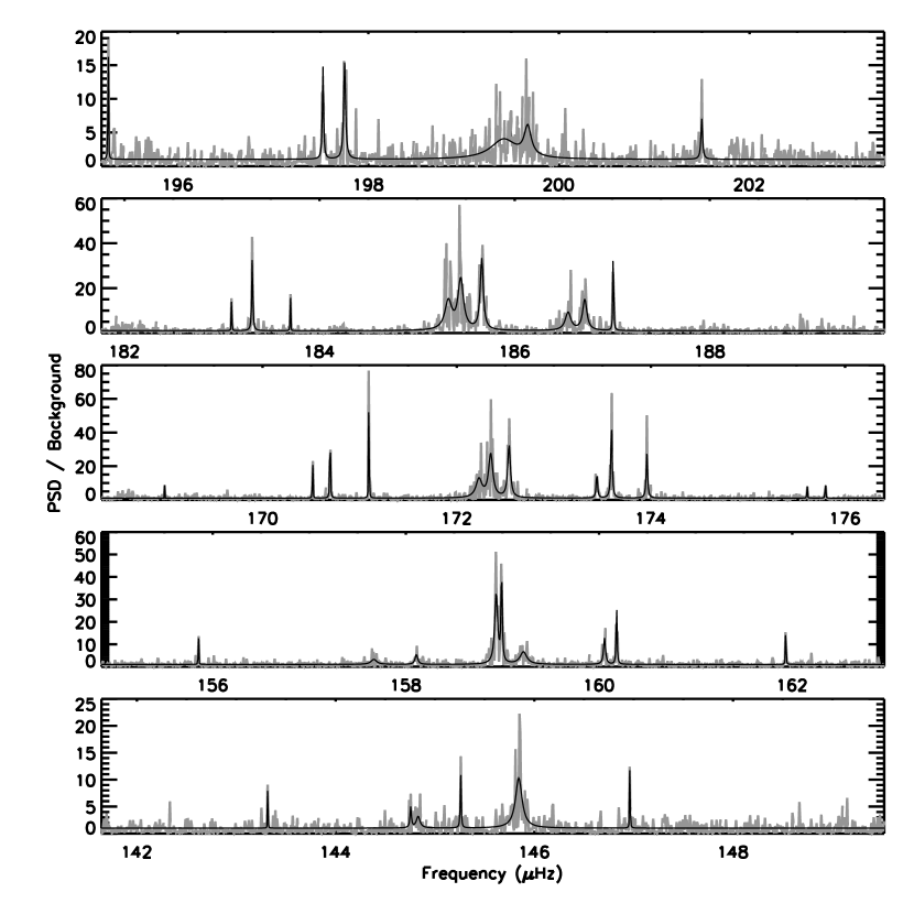
Supplementary Figure 1: Power spectrum density (PSD) of KIC 8684542. The grey curve corresponds to the PSD divided by the background noise. The black curve indicates the optimal fit to the PSD obtained in Sect. S1.

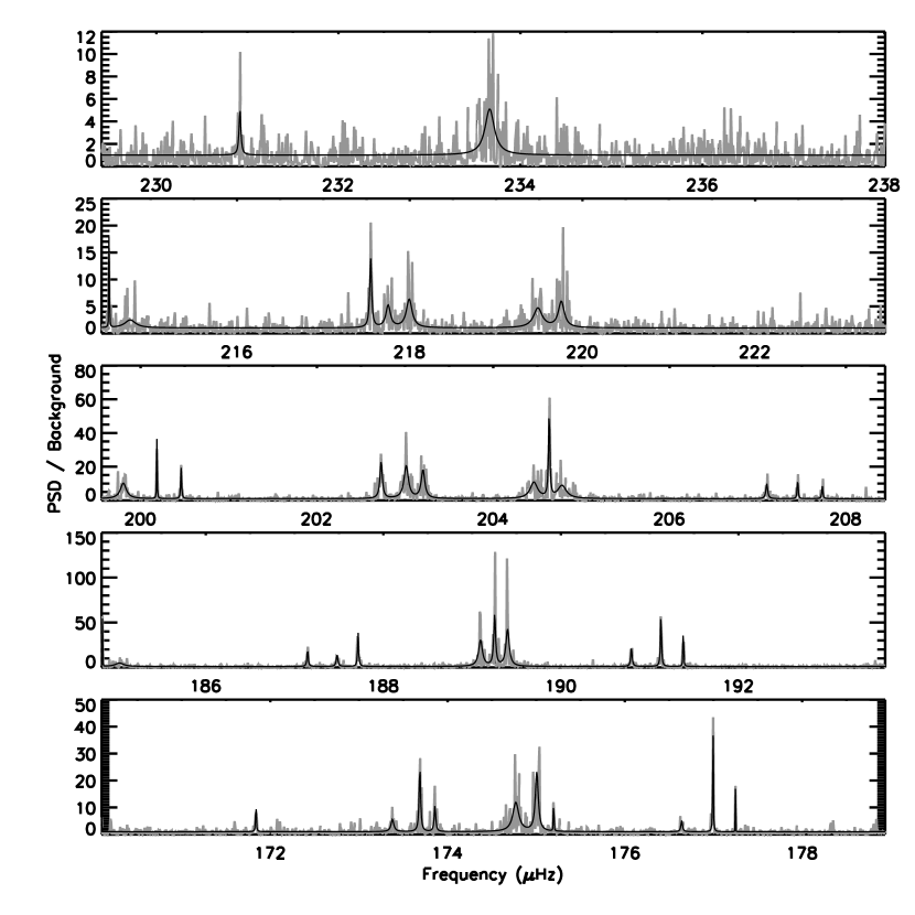
Supplementary Figure 2: Power spectrum density of KIC 11515377. Symbols have the same meaning as in Supplementary Figure 1.

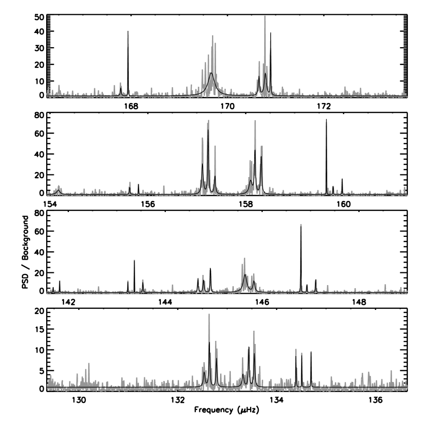
Supplementary Figure 3: Power spectrum density of KIC 7518143. Symbols have the same meaning as in Supplementary Figure 1.

Supplementary Figure 4: Observed rotational splittings as a function of the mode trapping. The mode trapping is measured by the parameter $\zeta$ ($\zeta\rightarrow 0$ for pure p modes, and $\zeta\rightarrow 1$ for pure g modes). The dashed lines correspond to the linear fits.

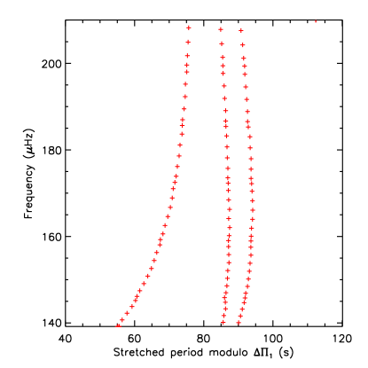
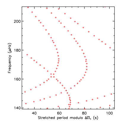
Supplementary Figure 5: Stretched period échelle diagrams of asymptotic mixed mode frequencies for two different field strengths. The left panel corresponds to a moderate magnetic shift ($\delta\!\omega_{\mathrm{g}}/(2\pi)=0.2\,\mathrm{\mu Hz}$) and the right panel to a strong magnetic shift ($\delta\!\omega_{\mathrm{g}}/(2\pi)=2\,\mathrm{\mu Hz}$).

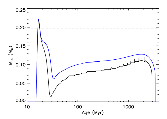
Supplementary Figure 6: Evolution of convective core mass during the main sequence for the best-fit model of KIC 11515377. Models were computed without core overshooting (black curve), or with overshooting extending over $0.2\,H_{p}$, where $H_{p}$ is the pressure scale height (blue curve). The dashed line indicates the layer of the hydrogen burning shell at current age.

Supplementary Tables

Supplementary Table 1: Properties of p and g modes of KIC 8684542, KIC 11515377, and KIC 7518143. These values were obtained by fitting an asymptotic expression of mixed modes to the $m=0$ observed frequencies (magnetic perturbations are not included at this stage). The last two lines give masses and radii derived from seismic scaling relations[2].

parameter	KIC 8684542	KIC 11515377	KIC 7518143
$\nu_{\rm max}$ ($\mu$Hz)	$176.8\pm 1.1$	$191.6\pm 1.0$	$156.3\pm 0.9$
$\Delta\nu$ ($\mu$Hz)	$13.484\pm 0.006$	$14.946\pm 0.008$	$12.374\pm 0.008$
$\alpha$	$(3.2\pm 0.4)\times 10^{-3}$	$(9.1\pm 0.3)\times 10^{-3}$	$(3.1\pm 0.4)\times 10^{-3}$
$\varepsilon_{\rm p}$	$1.275\pm 0.006$	$1.149\pm 0.008$	$1.234\pm 0.009$
$\Delta\Pi_{1}$ (s)	$80.16\pm 0.02$	$83.19\pm 0.04$	$78.49\pm 0.03$
$\varepsilon_{\rm g}$	$0.50\pm 0.02$	$0.50\pm 0.03$	$0.30\pm 0.03$
$q$	$0.122\pm 0.04$	$0.148\pm 0.004$	$0.117\pm 0.004$
$d_{01}$ ($\mu$Hz)	$-0.11\pm 0.02$	$0.09\pm 0.02$	$-0.08\pm 0.02$
$M/M_{\odot}$	$1.43\pm 0.07$	$1.60\pm 0.09$	$1.50\pm 0.08$
$R/R_{\odot}$	$5.23\pm 0.09$	$5.16\pm 0.09$	$5.65\pm 0.11$

Supplementary Table 2: Extracted mode frequencies for KIC 8684542, KIC 11515377 and KIC 7518143.

KIC 8684542
$143.318\pm 0.003$
$144.756\pm 0.009$
$144.829\pm 0.033$
$145.259\pm 0.006$
$145.844\pm 0.012$
$146.963\pm 0.005$
$155.852\pm 0.001$
$157.669\pm 0.020$
$158.110\pm 0.011$
$158.935\pm 0.008$
$158.992\pm 0.005$
$159.217\pm 0.016$
$160.057\pm 0.006$
$160.182\pm 0.004$
$161.934\pm 0.002$
$170.516\pm 0.001$
$170.696\pm 0.002$
$171.095\pm 0.001$
$172.229\pm 0.017$
$172.350\pm 0.010$
$172.539\pm 0.007$
$173.443\pm 0.005$
$173.594\pm 0.004$
$173.958\pm 0.004$
$175.608\pm 0.002$
$175.797\pm 0.001$
$180.760\pm 0.001$
$183.099\pm 0.002$
$183.310\pm 0.004$
$183.700\pm 0.001$
$185.315\pm 0.014$
$185.446\pm 0.013$
$185.663\pm 0.007$
$186.547\pm 0.013$
$186.718\pm 0.009$
$187.011\pm 0.002$
$194.882\pm 0.002$
$195.270\pm 0.001$
$197.524\pm 0.005$
$197.751\pm 0.006$
$199.420\pm 0.051$
$199.672\pm 0.023$
$201.499\pm 0.007$

KIC 11515377
$169.540\pm 0.001$
$171.837\pm 0.003$
$173.377\pm 0.010$
$173.687\pm 0.005$
$173.857\pm 0.006$
$174.770\pm 0.013$
$175.006\pm 0.008$
$175.197\pm 0.002$
$176.641\pm 0.010$
$176.994\pm 0.003$
$177.247\pm 0.001$
$179.111\pm 0.002$
$179.491\pm 0.004$
$184.837\pm 0.001$
$187.146\pm 0.004$
$187.480\pm 0.007$
$187.716\pm 0.004$
$189.094\pm 0.008$
$189.254\pm 0.005$
$189.399\pm 0.007$
$190.795\pm 0.005$
$191.127\pm 0.004$
$191.380\pm 0.002$
$193.974\pm 0.001$
$194.231\pm 0.005$
$199.804\pm 0.012$
$200.185\pm 0.002$
$200.460\pm 0.004$
$202.728\pm 0.007$
$203.013\pm 0.010$
$203.203\pm 0.010$
$204.461\pm 0.018$
$204.634\pm 0.005$
$204.780\pm 0.020$
$207.103\pm 0.007$
$207.453\pm 0.004$
$207.733\pm 0.007$
$214.520\pm 0.002$
$214.763\pm 0.040$
$217.547\pm 0.007$
$217.750\pm 0.018$
$217.994\pm 0.015$
$219.287\pm 0.015$
$219.491\pm 0.018$
$219.753\pm 0.018$
$230.918\pm 0.009$
$233.662\pm 0.019$

KIC 7518143
$132.535\pm 0.013$
$132.640\pm 0.006$
$132.784\pm 0.008$
$133.320\pm 0.015$
$133.437\pm 0.007$
$133.549\pm 0.008$
$134.393\pm 0.003$
$134.511\pm 0.002$
$134.698\pm 0.005$
$141.684\pm 0.002$
$141.823\pm 0.002$
$143.228\pm 0.001$
$143.363\pm 0.001$
$143.539\pm 0.004$
$144.676\pm 0.005$
$144.792\pm 0.007$
$144.933\pm 0.004$
$145.646\pm 0.013$
$145.830\pm 0.014$
$146.800\pm 0.001$
$146.925\pm 0.001$
$147.106\pm 0.003$
$155.630\pm 0.005$
$155.810\pm 0.002$
$157.115\pm 0.007$
$157.232\pm 0.005$
$157.371\pm 0.007$
$158.102\pm 0.026$
$158.189\pm 0.007$
$158.315\pm 0.006$
$159.649\pm 0.002$
$159.786\pm 0.001$
$159.971\pm 0.002$
$161.924\pm 0.184$
$167.786\pm 0.008$
$167.937\pm 0.004$
$169.664\pm 0.016$
$170.653\pm 0.008$
$170.786\pm 0.010$
$170.896\pm 0.004$

Supplementary Table 3: Extracted seismic parameters for KIC 8684542.

$\dfrac{\omega_{m=0}}{2\pi}$ ($\mu$Hz)	$\zeta$	$\dfrac{\delta\!\omega_{\rm R}}{2\pi}$ (nHz)	$\dfrac{\delta_{\rm asym}}{2\pi}$ (nHz)
$144.829\pm 0.033$	$0.781$	$251.6\pm 5.4$	$356.6\pm 66.2$
$157.669\pm 0.020$	$0.839$	-	$328.9\pm 42.7$
$158.992\pm 0.005$	$0.500$	$141.1\pm 9.0$	$169.3\pm 20.2$
$160.182\pm 0.004$	$0.819$	-	$287.8\pm 11.8$
$170.696\pm 0.002$	$0.869$	$289.9\pm 1.8$	$219.8\pm 4.7$
$172.350\pm 0.010$	$0.470$	$154.9\pm 18.1$	$68.7\pm 27.3$
$173.594\pm 0.004$	$0.794$	$257.5\pm 6.8$	$213.7\pm 10.8$
$175.797\pm 0.001$	$0.951$	-	$255.3\pm 3.3$
$183.310\pm 0.004$	$0.915$	$300.7\pm 1.9$	$178.8\pm 7.3$
$185.446\pm 0.013$	$0.518$	$173.7\pm 16.2$	$85.7\pm 31.4$
$186.718\pm 0.009$	$0.687$	$231.7\pm 13.4$	$121.7\pm 23.2$
$194.882\pm 0.002$	$0.956$	-	$139.2\pm 3.7$
$197.751\pm 0.006$	$0.815$	-	$81.1\pm 14.0$

Supplementary Table 4: Extracted seismic parameters for KIC 11515377.

$\dfrac{\omega_{m=0}}{2\pi}$ ($\mu$Hz)	$\zeta$	$\dfrac{\delta\!\omega_{\rm R}}{2\pi}$ (nHz)	$\dfrac{\delta_{\rm asym}}{2\pi}$ (nHz)
$173.687\pm 0.005$	$0.693$	$240.0\pm 12.1$	$-140.0\pm 15.5$
$175.006\pm 0.008$	$0.547$	$213.7\pm 12.7$	$-46.1\pm 20.2$
$176.994\pm 0.003$	$0.907$	$302.8\pm 10.2$	$-99.8\pm 11.5$
$179.491\pm 0.004$	$0.965$	-	$-111.0\pm 9.2$
$187.480\pm 0.007$	$0.834$	$284.9\pm 6.1$	$-97.9\pm 14.6$
$189.254\pm 0.005$	$0.427$	$152.5\pm 10.7$	$-14.1\pm 15.3$
$191.127\pm 0.004$	$0.851$	$292.5\pm 5.4$	$-79.6\pm 8.9$
$200.185\pm 0.002$	$0.940$	$327.9\pm 12.9$	$-106.2\pm 13.8$
$203.013\pm 0.010$	$0.636$	$237.3\pm 11.8$	$-94.3\pm 23.5$
$204.634\pm 0.005$	$0.541$	$159.6\pm 26.8$	$-28.5\pm 28.5$
$207.453\pm 0.004$	$0.927$	$315.4\pm 9.5$	$-70.2\pm 12.4$
$217.750\pm 0.018$	$0.639$	$223.2\pm 16.8$	$40.8\pm 39.8$
$219.491\pm 0.018$	$0.514$	$233.0\pm 11.5$	$59.5\pm 43.1$

Supplementary Table 5: Extracted seismic parameters for KIC 7518143.

$\dfrac{\omega_{m=0}}{2\pi}$ ($\mu$Hz)	$\zeta$	$\dfrac{\delta\!\omega_{\rm R}}{2\pi}$ (nHz)	$\dfrac{\delta_{\rm asym}}{2\pi}$ (nHz)
$132.640\pm 0.006$	$0.705$	$124.4\pm 15.4$	$39.4\pm 20.1$
$133.437\pm 0.007$	$0.629$	$114.3\pm 16.8$	$-4.3\pm 21.6$
$134.511\pm 0.002$	$0.893$	$152.2\pm 5.6$	$69.3\pm 6.8$
$141.823\pm 0.002$	$0.971$	-	$51.5\pm 4.2$
$143.363\pm 0.001$	$0.932$	$155.7\pm 3.8$	$41.4\pm 4.0$
$144.792\pm 0.007$	$0.721$	$128.6\pm 6.3$	$25.9\pm 14.9$
$146.925\pm 0.001$	$0.890$	$153.1\pm 3.0$	$56.6\pm 4.2$
$155.630\pm 0.005$	$0.924$	-	$43.7\pm 11.1$
$157.232\pm 0.005$	$0.638$	$127.9\pm 10.0$	$22.1\pm 14.3$
$158.189\pm 0.007$	$0.614$	$106.1\pm 26.5$	$39.3\pm 29.6$
$159.786\pm 0.001$	$0.918$	$161.1\pm 3.0$	$48.6\pm 4.0$
$167.937\pm 0.004$	$0.915$	-	$12.3\pm 13.6$
$170.786\pm 0.010$	$0.671$	$121.5\pm 9.1$	$-23.1\pm 21.5$

Supplementary Table 6: Average rotation rates in the core $\langle\Omega\rangle_{\rm g}$ and in the envelope $\langle\Omega\rangle_{\rm p}$.

KIC ID	$\langle\Omega\rangle_{\rm g}/(2\pi)$	$\langle\Omega\rangle_{\rm p}/(2\pi)$
	(nHz)	(nHz)
8684542	$667\pm 43$	$-24\pm 15$
11515377	$669\pm 46$	$52\pm 14$
7518143	$338\pm 53$	$31\pm 17$

Supplementary Table 7: Magnetic field properties for the three red giants. These values were obtained by fitting an asymptotic expression of mixed modes that includes a magnetic perturbation to the observed mode frequencies of KIC 8684542, KIC 11515377, and KIC 7518143.

parameter	KIC 8684542	KIC 11515377	KIC 7518143
$\Delta\Pi_{1}$ (s)	$80.47\pm 0.11$	$83.56\pm 0.14$	$78.52\pm 0.08$
$\delta\!\omega_{\mathrm{g}}/(2\pi)$ (nHz)	$195\pm 45$	$126\pm 60$	$<35$
$a$	$0.47\pm 0.12$	$-0.24_{-0.23}^{+0.08}$	$>0.24$
$\langle B_{r}^{2}\rangle^{1/2}$ (kG)	$102\pm 12$	$98\pm 24$	$<41$

References

- [1] Deheuvels, S. et al. Seismic Evidence for a Rapidly Rotating Core in a Lower-giant-branch Star Observed with Kepler. \JournalTitleApJ 756, 19 (2012).
- [2] Gehan, C., Mosser, B., Michel, E., Samadi, R. & Kallinger, T. Core rotation braking on the red giant branch for various mass ranges. \JournalTitleA&A 616, A24 (2018).
- [3] Marques, J. P. et al. Seismic diagnostics for transport of angular momentum in stars. I. Rotational splittings from the pre-main sequence to the red-giant branch. \JournalTitleA&A 549, A74 (2013).
- [4] Gough, D. O. & McIntyre, M. E. Inevitability of a magnetic field in the Sun’s radiative interior. \JournalTitleNature 394, 755–757 (1998).
- [5] Fuller, J., Piro, A. L. & Jermyn, A. S. Slowing the spins of stellar cores. \JournalTitleMNRAS 485, 3661–3680 (2019).
- [6] Gouhier, B., Jouve, L. & Lignières, F. Angular momentum transport in a contracting stellar radiative zone embedded in a large scale magnetic field. \JournalTitlearXiv e-prints arXiv:2201.02645 (2022).
- [7] Unno, W., Osaki, Y., Ando, H., Saio, H. & Shibahashi, H. Nonradial oscillations of stars (University of Tokyo Press, Tokyo, 1989).
- [8] Gough, D. O. & Thompson, M. J. The effect of rotation and a buried magnetic field on stellar oscillations. \JournalTitleMNRAS 242, 25–55 (1990).
- [9] Hasan, S. S., Zahn, J. P. & Christensen-Dalsgaard, J. Probing the internal magnetic field of slowly pulsating B-stars through g modes. \JournalTitleA&A 444, L29–L32 (2005).
- [10] Gomes, P. & Lopes, I. Core magnetic field imprint in the non-radial oscillations of red giant stars. \JournalTitleMNRAS 496, 620–628 (2020).
- [11] Bugnet, L. et al. Magnetic signatures on mixed-mode frequencies. I. An axisymmetric fossil field inside the core of red giants. \JournalTitleA&A 650, A53 (2021).
- [12] Loi, S. T. Topology and obliquity of core magnetic fields in shaping seismic properties of slowly rotating evolved stars. \JournalTitleMNRAS 504, 3711–3729 (2021).
- [13] Borucki, W. J. et al. Kepler Planet-Detection Mission: Introduction and First Results. \JournalTitleScience 327, 977 (2010).
- [14] Mathis, S. et al. Probing the internal magnetism of stars using asymptotic magneto-asteroseismology. \JournalTitleA&A 647, A122 (2021).
- [15] Deheuvels, S., Ouazzani, R. M. & Basu, S. Near-degeneracy effects on the frequencies of rotationally-split mixed modes in red giants. \JournalTitleA&A 605, A75 (2017).
- [16] Supplementary Materials.
- [17] Dziembowski, W. A. & Goode, P. R. Effects of Differential Rotation on Stellar Oscillations: A Second-Order Theory. \JournalTitleApJ 394, 670 (1992).
- [18] Paxton, B. et al. Modules for Experiments in Stellar Astrophysics (MESA). \JournalTitleApJS 192, 3 (2011).
- [19] Mosser, B. et al. Period spacings in red giants. IV. Toward a complete description of the mixed-mode pattern. \JournalTitleA&A 618, A109 (2018).
- [20] Takata, M. Asymptotic analysis of dipolar mixed modes of oscillations in red giant stars. \JournalTitlePASJ 68, 109 (2016).
- [21] Fuller, J., Cantiello, M., Stello, D., Garcia, R. A. & Bildsten, L. Asteroseismology can reveal strong internal magnetic fields in red giant stars. \JournalTitleScience 350, 423–426 (2015).
- [22] Stello, D. et al. A prevalence of dynamo-generated magnetic fields in the cores of intermediate-mass stars. \JournalTitleNature 529, 364–367 (2016).
- [23] Donati, J. F. & Landstreet, J. D. Magnetic Fields of Nondegenerate Stars. \JournalTitleARA&A 47, 333–370 (2009).
- [24] Braithwaite, J. & Spruit, H. C. Magnetic fields in non-convective regions of stars. \JournalTitleRoyal Society Open Science 4, 160271 (2017).
- [25] Becerra, L., Reisenegger, A., Valdivia, J. A. & Gusakov, M. E. Evolution of random initial magnetic fields in stably stratified and barotropic stars. \JournalTitleMNRAS 511, 732–745 (2022).
- [26] Cantiello, M., Fuller, J. & Bildsten, L. Asteroseismic Signatures of Evolving Internal Stellar Magnetic Fields. \JournalTitleApJ 824, 14 (2016).
- [27] Brun, A. S., Browning, M. K. & Toomre, J. Simulations of Core Convection in Rotating A-Type Stars: Magnetic Dynamo Action. \JournalTitleApJ 629, 461–481 (2005).
- [28] Aurière, M. et al. Weak magnetic fields in Ap/Bp stars. Evidence for a dipole field lower limit and a tentative interpretation of the magnetic dichotomy. \JournalTitleA&A 475, 1053–1065 (2007).
- [29] Deheuvels, S. et al. Seismic constraints on the radial dependence of the internal rotation profiles of six Kepler subgiants and young red giants. \JournalTitleA&A 564, A27 (2014).
- [30] Mosser, B., Vrard, M., Belkacem, K., Deheuvels, S. & Goupil, M. J. Period spacings in red giants. I. Disentangling rotation and revealing core structure discontinuities. \JournalTitleA&A 584, A50 (2015).