A New Outlook on the Profitability of Rogue Mining Strategies in the Bitcoin Network

1 Abstract

Many of the recent works on the profitability of rogue mining strategies hinge on a parameter called gamma ($\gamma$) that measures the proportion of the honest network attracted by the attacker to mine on top of his fork. These works, see [GP18a] and [GP18], have surmised conclusions based on premises that erroneously treat $\gamma$ to be constant. In this paper, we treat $\gamma$ as a stochastic process and attempt to find its distribution through a Markov analysis. We begin by making strong assumptions on gamma’s behaviour and proceed to translate them mathematically in order to apply them in a Markov setting. The aforementioned is executed in two separate occasions for two different models. Furthermore, we model the Bitcoin network and numerically derive a limiting distribution whereby the relative accuracy of our models is tested through a likelihood analysis. Finally, we conclude that even with control of 20% of the total hashrate, honest mining is the strongly dominant strategy.

2 Introduction

In this section we aim to explain various fundamental concepts used in our research below and how they are interrelated. To begin with, a description of the three rogue mining strategies investigated in this paper is warranted. Furthermore, the concept of a difficulty adjustment which is exploited in these strategies is of paramount importance. To accompany the aforementioned, it is also essential to explain the importance of $gamma$ in these strategies.

Mining a block entails ”finding” the target cryptographic hash of the block. The target hash is a hash that begins with a predetermined number of zeros. A miner concatenates the version of the current Bitcoin software, the timestamp of the block, the root of its’ transaction’s merkle tree, the difficulty target and the nonce and inputs them in the SHA-256 hashing function to obtain an output. The nonce is the only variable quantity out of these six elements. Hence, the miner only varies the nonce and inputs it in the SHA-256 hashing function in the hopes of obtaining the target hash. ”Obtaining the target hash” does not mean having the identical hash being output from the SHA-256 algorithm; it means obtaining a hash that has the same or more leading zeros. The difficulty is defined as the number of leading zeros contained in the target hash. The Bitcoin network demands a block be mined in 10 minutes and after 2016 blocks the network evaluates whether these blocks have been approximately mined in 20,160 minutes. The difficulty adjustment primarily depends on the number of miners or more precisely the hashing power of the sum of all miners. If the totality of the miners have taken more time to do so than the network adjusts the difficulty by reducing the number of leading zeros and if not the analogous occurs.

In this paper we make use of three rogue strategies. These are: Selfish Mining (SM), Least-Stubborn Mining (LSM) and Equal Fork Stubborn Mining (EFSM). The two latter ones are slight modifications of the popular Selfish Mining attack. SM is a strategy that targets the difficulty adjustment of the protocol by invalidating ”honest” blocks through broadcasting a chain of secretly mined blocks which results in slowing down the network and hence the difficulty becomes easier even though the hashing power has not changed. Henceforth, the revenue of a miner per unit time increases. EFSM and LSM differentiate from SM only in terms of the timing on when the secret chain is revealed as well as the fact that the miner also has the choice to strategically reveal blocks instead of the entire chain when it comes to EFSM and LSM. For a complete a description of the strategies we refer the reader to [GP18a] and [GP18].

The parameter $\gamma$ appears when a fork between a rogue chain and an honest chain occurs (see [Nay+16]). In such scenarios, there exists a fraction of honest miners (in other words $\gamma$) that mine on top of the rogue chain. This parameter is instrumental in the investigation of the optimality of rogue mining strategies; thence, we investigate its behaviour in this paper.

3 Bitcoin Network

We are going to outline and motivate the construction of a Bitcoin network, mirroring many aspects of the existing network. This will be used as a proxy to test the relative fitness of our analytical Markov models for the distribution of $\gamma$.

Tools from graph theory will be used to construct a numerical model that will be used to stochastically simulate the Bitcoin network using a series of increasing times $\tau$ (see code excerpt 2), that represent the real times since the first instance where two nodes ping the network and the response in terms of $\gamma$ is recorded and stored in an array. By sampling from such a sequence, of times, we obtain a time series of values of $\gamma$, whence we compute the transition probabilities between optimal mining strategies in the Markov chain model for gamma, and as a by product, we get its limiting distribution (see code excerpt 1).

The nodes in the network are meant to correspond to mining pools across the world, each in a specific continent. The amount of nodes in each continent is determined by the fraction of the hash rate contributed to the Bitcoin network by each continent respectfully [Aok+19] (see code excerpt 7).

3.1 Construction

The Bitcoin network at any given time $t\geq 0$ will be modelled by a weighted graph

$$\mathcal{G}_{t}=(V_{t},E_{t})$$

with $V_{t}=\{1,2,3\dots,100\}$ vertices corresponding to nodes on the network, and $E_{t}=\left\{\{i,j\}|\forall 1\leq i<j\leq 100\right\}$ edges, with a (stochastic - its precise nature will be explained later) weight function

$$\mathcal{W}_{t}:E_{t}\rightarrow\mathbb{R}$$

that measures the latency of nodes between themselves in microseconds.

Key assumptions on the latencies between the nodes that will be explored further below are:

• network topology

• historical latency

• skew normality of latency distribution

• time separation between the measurements

To account for geographical separation between the nodes, values for the mean latencies between continents in the Bitcoin network in 2019 (see [Aok+19]) were used in the weights of the graph $\mathcal{G}_{t}$.

Additionally, the topology of the network, that is the combinatorial properties of the underlying graph used to model the network itself (see [Tru13], p.76), will have an impact on the connectivity of the nodes therein. More specifically, the notion of eigenvalue centrality plays a crucial role in determining the weights of the network. The utility of this metric lies in that heuristically, nodes with high centrality are connected to proportionately more nodes with high scores [New08]. To make this mathematically precise, one takes the adjacency matrix of the graph upon initialisation of the graph’s weights in the simulation at a given time; some of the weighs may take the value $1E7$, which is to be interpreted that the connection between the nodes is non existent at that moment. Then, one computes the adjacency matrix of the graph, defined by:

$$\bf{A}_{ij}=\left\{\begin{array}[]{ll}1\text{ if }\mathcal{W}({i,j)}<1E7\\ 0\text{ otherwise}\\ \end{array}\right.$$

for $\{i,j\}\in V$. This is then used to compute the centrality score vector $\bf{\Omega}$ which satisfies:

$$\lambda\bf{\Omega}=A.\bf{\Omega}$$

which satisfies $\bf{\Omega}(i)\geq 0$ for all $i$ vertices in the graph and

$$\sum_{i\in V}\bf{\Omega}(i)=1$$

We remark that its existence is guaranteed by the Perron - Frobenius Theorem[New08]. With regards to modelling latencies on the network, we observe that on a mining network following the Bitcoin protocol, the latencies follow a multimodal distribution (see [Gen+18], figure 3). For this reason, it will be assumed that the weights of the network will follow a skew-normal distribution with shape parameter $\alpha$ depending on the combined eigenvector centrality of the nodes comprising an edge.

3.2 Modelling Assumptions

Before diving into the modeling assumptions, it is important to state that mining is a Markov process, see [GP20]. Let $\gamma_{n}$ for $n\in\mathbb{N}$ represent the process modelling $\gamma$ in discrete time, and consider the modified stochastic process indexed by $\mathbb{N}$:

$$X_{n}=\bigcup_{k\in T}\mathbf{1}_{A_{k}}(\gamma_{n}):\mathbb{N}\rightarrow\Xi$$

where

$$\mathbf{1}_{A_{k}}(x)=\begin{cases}A_{k}&\text{if $x\in A_{k}$,}\\ \emptyset&\text{otherwise}\end{cases}$$

and $T\subset\mathbb{N},$ $|T|<\infty$, and $\Xi=\{A_{k}:k\in T\}$ such that

$$A_{i}\bigcap A_{j}=\emptyset\text{ }\forall i\neq j\in T$$

and $\bigcup_{k\in T}A_{k}=[0,1]$ For our following model to predict transition probabilities between strategies we require to satisfy the following ideas:

1. The probability that $\gamma$ jumps to an interval that is further away to be smaller than the probability of it jumping to interval nearby

2. The probability that $\gamma$ jumps to an interval with greater length to be greater than the probability that it jumps to an interval of smaller length.

The intuitive idea behind the above assumptions is the following. As mentioned previously $\gamma$ represents the proportion of people that follow our chain. We want the process of say a change of $\gamma=0.2$ to $\gamma=0.21$ to be more probable than a change from $\gamma=0.2$ to $\gamma=0.6$. In deed, it seems quite improbable that 20% of people following our chain turn to 60% compare to 21%. Furthermore, since we give $\gamma$ a range rather than a fixed value in the Markov models, it also makes sense that if we jump to greater range of $\gamma$ we are giving ourselves more leeway than if we confined ourselves to a very small one. The above assumptions can be mathematically stated as:

$$\mathbb{P}(X_{n_{1}}=[x_{1},x_{2}]|X_{n-1}=[y_{1},y_{2}])\leq\mathbb{P}(X_{n_{2}}=[x_{3},x_{4}]|X_{n-1}=[y_{1},y_{2}]),$$

if

$$d_{p}([x_{3},x_{4}],[y_{1},y_{2}])\leq d_{p}([x_{1},x_{2}],[y_{1},y_{2}])\text{, and }d(x_{1},x_{2})=d(x_{3},x_{4})$$

Where $d_{p}(X,Y)$ is a metric defined in the following way:

$$d_{p}:\mathcal{P}([0,1])\times\mathcal{P}([0,1])\longrightarrow\mathbb{N}$$

$$d_{p}([x_{1},x_{2}],[y_{1},y_{2}])=d\Big{(}x_{1}+\frac{x_{2}-x_{1}}{2},y_{1}+\frac{y_{2}-y_{1}}{2}\Big{)}$$

Where $d(.,.)$ is the standard metric. Moreover, we also require

$$\mathbb{P}(X_{n_{1}}=[x_{1},x_{2}]|X_{n-1}=[y_{1},y_{2}])\leq\mathbb{P}(X_{n_{2}}=[x_{3},x_{4}]|X_{n-1}=[y_{1},y_{2}]),$$

if

$$d_{p}([x_{3},x_{4}],[y_{1},y_{2}])=d_{p}([x_{1},x_{2}],[y_{1},y_{2}])\text{, and }d(x_{1},x_{2})\leq d(x_{3},x_{4})$$

4 Exploration of Models

4.1 1st Markov Model

Based on the above, the following probability model will be used to compute transition probabilities:

$$\mathbb{P}(X_{n}=[x_{1},x_{2}]|X_{n-1}=[y_{1},y_{2}])=\frac{\displaystyle\int_{x_{1}}^{x_{2}}1-d_{p}([x_{1},x_{2}],[y_{1},y_{2}])\;\mathrm{d}x}{\displaystyle\sum_{\xi\in\Xi}\displaystyle\int_{x_{1}}^{x_{2}}1-d_{p}([x_{1},x_{2}],\xi)\;\mathrm{d}x}$$ (1)

The interval $[0,1]$ is partitioned into disjoint intervals as will be explained below which is represented by the set $\Xi$; the denominator is a sum over all such disjoint intervals.
Fixing the collection of nodes applying this strategy at an hashrate of 20%, according to [GP18a], $\gamma$ is partitioned in the following way:

$$\Xi=\{[0,0.675],[0.675,0.76],[0.76,0.761],[0.761,1]\}$$

The set $\Xi$ as mentioned previously is the set encapsulating the way $\gamma$ is partitioned in correspondence with the mining strategies. From left to right we have: honest mining (HM), selfish mining (SM), Lead-Stubborn mining (LSM), Equal Fork Stubborn mining (EFSM). We will compute the transition probabilities. The same process is analogously applied for all other states.

Representing the results in a transition matrix, we obtain

$\mathbf{P_{1}}$ =

$$\begin{bmatrix}&0.81&0.06&0&0.13\\ &0.59&0.12&0.01&0.28\\ &0.57&0.12&0&0.31\\ &0.5&0.11&0&0.39\\ \end{bmatrix}$$

The chain is irreducible therefore the limiting distribution $\mathbf{\pi}$ can be obtained by solving the following equation

$$\mathbf{\pi}=\bf{\pi}\mathbf{P_{1}}$$

The matrix $\mathbf{P_{1}}$ has rank equal to $3$ which signifies that the solution has a dependency on one variable. This variable can be chosen to be unique since we require $\sum_{i=1}^{4}\mathbf{\pi}_{i}=1$. Solving the above equation and taking into consideration the aforementioned we obtain the limiting distribution where each term is rounded to significant figures:

$$\mathbf{\pi_{1}}=\Big{(}0.73\text{ }0.08\text{ }0\text{ }0.19\Big{)}\\$$

4.2 2nd Markov model

Upon exploring the first Markov model, we proceed with another candidate for the distribution of gamma. This will be motivated by choice of ’Gaussian’, or squared exponential kernel

$$\kappa(x,y)=\exp\left(-\frac{1}{2}\left(\frac{x-y}{l}\right)^{2}\right)$$

where $l=\frac{1}{4}$ is chosen to be the characteristic length scale of the process $\gamma_{t}$.

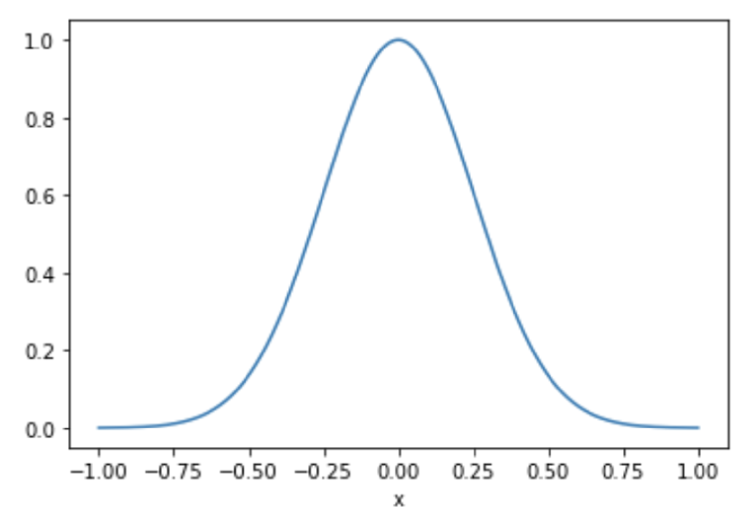
Figure 1: Plot of $\exp(-\frac{1}{2}(\frac{x}{l})^{2})$ on $[-1,1]$, with $l=\frac{1}{4}$.

Once again, pertaining to the above assumptions, the transition probabilities will also be estimated as

$$\mathbb{P}(X_{n}=[x_{1},x_{2}]|X_{n-1}=[y_{1},y_{2}])=\frac{\displaystyle\int_{x_{1}}^{{x_{2}}}\int_{{y_{1}}}^{{y_{2}}}\kappa(x,y)\;\mathrm{d}x\;\mathrm{d}y}{\displaystyle\int_{0}^{1}\int_{{y_{1}}}^{{y_{2}}}\kappa(x,y)\;\mathrm{d}x\;\mathrm{d}y}$$ (2)

Heuristically, this is used to determine how close two points have to be to influence each other significantly. This model allows for interiors of intervals to interfere with each other and make contributions to the total probability of a specific transition. Using figure 1 as a guide, one notices that the length scale $l$ is chosen in a fashion such that if the separation of two points is greater that half the length of the domain of $\gamma$, then, their contribution to the probability becomes minimal.

It is clear that the farther apart two disjoint intervals are, one possible way to gauge this is using their Hausdorff distance, the probability given by the model will be expected to be less than if the intervals were close so that the mean separation between points in the intervals is within the ’support’ of the kernel.

Also, by the mean value theorem for integrals, one obtains up to a constant of proportionality that for intervals $[x_{1},x_{2}]$ and $[x_{1}^{\prime},x_{2}^{\prime}]$

$$\mathbb{P}(X_{n}=[x_{1},x_{2}]|X_{n-1}=[y_{1},y_{2}])\sim(x_{2}-x_{1})\displaystyle\int_{{y_{1}}}^{{y_{2}}}\kappa(\xi_{1},y)\;\mathrm{d}y$$

$$\mathbb{P}(X_{n}=[x_{1}^{\prime},x_{2}^{\prime}]|X_{n-1}=[y_{1},y_{2}])\sim(x_{2}^{\prime}-x_{1}^{\prime})\displaystyle\int_{{y_{1}}}^{{y_{2}}}\kappa(\xi_{2},y)\;\mathrm{d}y$$

where $\xi_{1}=(x_{1},x_{2})$ and $\xi_{2}\in(x_{1}^{\prime},x_{2}^{\prime})$. If now one chooses the above intervals such that $d(\xi_{1},[y_{1},y_{2}])\approx d(\xi_{2},[y_{1},y_{2}])$, then the relative lengths of the intervals drives the relative behaviour of the probabilities of landing in said intervals. Thus, the modelling assumptions laid out above are adequately addressed by this model.

The transition matrix and transition diagram are as follows:

$$\mathbf{P_{2}}=\begin{bmatrix}&0.84&0.07&0&0.09\\ &0.50&0.15&0.002&0.348\\ &0.43&0.16&0.002&0.408\\ &0.32&0.158&0.002&0.52\\ \end{bmatrix}$$

Applying the exact same procedure as we did with the previous stochastic matrix, we obtain the following limiting distribution

$$\mathbf{\pi_{2}}=\Big{(}0.7\text{ }0.1\text{ }0\text{ }0.2\Big{)}$$

5 Numerical Results

In the simulation, the network will be sampled at constant intervals of length one unit of time, staying consistent with the first two Markov Models. Thus, in the above framework, we take $\tau$ to be

$$\mathbf{\tau}=\{0,1,2,\dots,T-1\}$$

where $T$ is some predefined constant. For the transition probabilities, a value of $T=1000$ will be used.

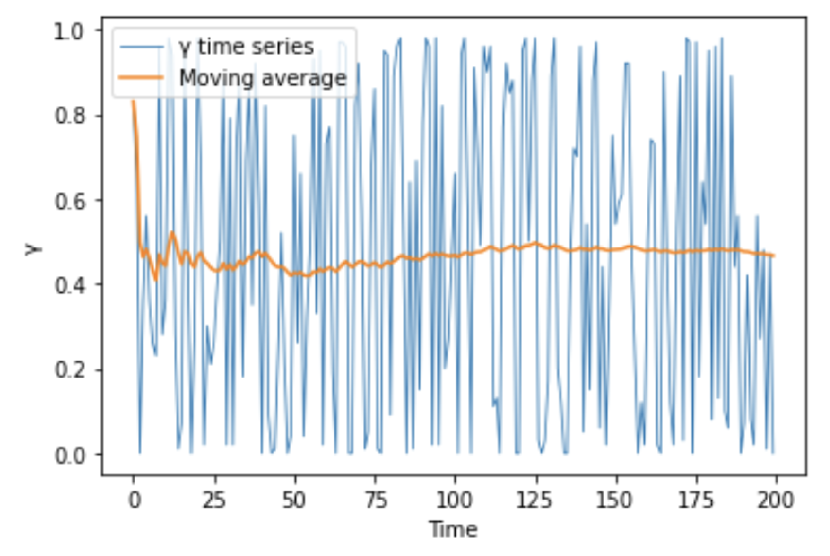
Figure 2: Times series of $\gamma$ from time with $T=200$ uniformly spaced samples, including the moving average

Below are the matrix of frequencies of each transition and the resulting transition probability matrix using $T=5000$ samples; though a time series for $\gamma$ (see figure 2) with $T=200$ is included for convenience.

$$\mathbf{N}=\begin{bmatrix}&2977&205&0&690\\ &213&10&1&34\\ &8&1&0&6\\ &676&42&0&136\\ \end{bmatrix}$$

$$\mathbf{P_{3}}=\begin{bmatrix}&0.77&0.05&0.0&0.18\\ &0.83&0.036&0.004&0.13\\ &0.53&0.07&0.0&0.4\\ &0.79&0.05&0.0&0.16\\ \end{bmatrix}$$

The chain represented by the above matrix is irreducible therefore we can apply the same techniques to derive a limiting distribution as we did for the previous two matrices. We obtain:

$$\mathbf{\pi_{3}}=\Big{(}0.78\text{ }0.05\text{ }0\text{ }0.17\Big{)}$$

6 Likelihood Analysis

Using the numerical model as a proxy for real data $\mathbf{N}$, we will perform a likelihood analysis to compare the Markov models through their transition probability matrices $\mathbf{P_{1}},\mathbf{P_{2}}$.

Formally, we consider the parameter space of Markov models

$$\Theta=\left\{\mathbf{P}\in\mathbb{R}^{4\times 4}_{\geq 0}\bigg{|}\forall 0\leq i\leq 3,\displaystyle\sum_{0\leq j\leq 3}\mathbf{P}_{ij}=1\right\}$$

Now, the likelihoods of the models $\mathbf{P_{1}},\mathbf{P_{2}}$ given the time series for $\mathbf{\gamma}$, yielding $\mathbf{N}$ are computed using the Markov Property:

$$\mathcal{L}(\theta|N)=\displaystyle\prod_{0\leq i,j\leq 3}\mathbf{P}_{ij}^{\mathbf{N}_{ij}}\times\mathbb{P}(\gamma_{0}\in\Xi_{0})$$

we will see that the precise value of $\mathbb{P}(\gamma_{0}\in\Xi_{0})$ is irrelevant, so long as it is uniform across all models - an assumption we will make henceforth. Following [Dav03], we define for a model $\theta\in\Theta$, its Relative Ratio as follows:

$$R\mathcal{L}(\theta|\mathbf{N})=-\log\left(\frac{\mathcal{L}(\mathbf{\theta}|\mathbf{N})}{\displaystyle\sup_{\theta\in\Theta}\mathcal{L}(\mathbf{\theta}|\mathbf{N})}\right)=-\log\left(\frac{\mathcal{L}(\mathbf{\theta}|\mathbf{N})}{\mathcal{L}(\mathbf{\hat{\theta}}|\mathbf{N})}\right)$$

$$=-\left(\displaystyle\sum_{i,j}\mathbf{N}_{ij}\log(\mathbf{\theta}_{ij})-\displaystyle\sum_{i,j}\mathbf{N}_{ij}\log(\mathbf{\hat{\theta}}_{ij})\right)\in[0,\infty]$$

where $\hat{\theta}=P_{3}$, a known result in likelihood optimisation. Note that if $\mathcal{L}(\mathbf{\theta_{1}}|\mathbf{N})<\mathcal{L}(\mathbf{\theta_{2}}|\mathbf{N})$, then we have $R\mathcal{L}(\theta_{1}|\mathbf{N})>R\mathcal{L}(\theta_{2}|\mathbf{N})$. We now compute the log-relative likelihoods of models $\theta=\mathbf{P}_{1},\mathbf{P}_{2}$:

$R\mathcal{L}(\mathbf{P}_{1}|\mathbf{N})$	$R\mathcal{L}(\mathbf{P}_{2}|\mathbf{N})$
157	512

Table 1: Relative likelihoods of Markov models given data $N$.

7 Conclusion

Now that we have computed the limiting distributions from the three models discussed above, it is time to give them an interpretation. This will be achieved through the Ergodic theorem for Markov chains (see [NN98]), where for an irreducible and aperiodic homogeneous Markov chain $\{X_{n}\}_{n\in\mathbb{N}}$ with limiting distribution $\mathbf{\pi}$, with probability one the ratio counting the ratio of time spent in state $i$

$$V_{i}(n)=\displaystyle\frac{1}{n}\sum_{k=1}^{n}\mathbf{1}_{\{X_{k}=i\}}\rightarrow\frac{1}{\pi_{i}}$$

as $n\rightarrow\infty$.

Applying the above result to our models which can be seen to satisfy the above conditions, the limiting distributions

$$\mathbf{\pi_{1}}=\Big{(}0.73\text{ }0.08\text{ }0\text{ }0.19\Big{)}\\$$

$$\mathbf{\pi_{2}}=\Big{(}0.7\text{ }0.1\text{ }0\text{ }0.2\Big{)}$$

$$\mathbf{\pi_{3}}=\Big{(}0.78\text{ }0.05\text{ }0\text{ }0.17\Big{)}$$

are taken to measure as measuring the fraction of time spent in each optimal strategy for $\gamma$ in the long run, where optimality is taken in the sense of [GP18].

The log-likelihood analysis in section 6, the first model, namely $\mathbf{P_{1}}$ achieved a higher relative likelihood than the model $\mathbf{P_{2}}$, due to the relative log likelihoods computed in table 1.

We note that this observed difference with respect to the numerical data is due to the different theoretical premises they were derived from. For instance, the first model collapsed the intervals for $\gamma$ into their midpoints, whereas the second model exploited the non linear interaction of all of the interiors of said intervals, provided by the kernel $\kappa(x,y)$. Although, as discussed the paper, the qualitative features were broadly similar for they were meant to model the same underlying stochastic process $\gamma$.

Moreover, we see that even if the attacker has a hashrate of 20% in the Bitcoin network, the limiting distributions $\mathbf{\pi_{1}},\mathbf{\pi_{2}},\mathbf{\pi_{3}}$ show that honest mining is strongly dominant in the long run, where it is used more than $70\%$ of the time spent mining, as opposed to rogue mining strategies.

8 Author Contribution Statement

Y.P. conceived of the presented idea, namely the construction of Markov models for $\gamma$. Y.P. developed the theoretical formalism for the first analytical model and performed the calculations of the transition matrices and limiting distributions.

P.T. conceived of the theoretical formalism of second analytical model and the numerical model. P.T. produced the code in the appendix to perform numerical simulations and performed the log-likelihood analysis of the analytical models using the numerical model as a benchmark.

Both authors discussed the results and contributed to the final manuscript.

9 Appendix

9.1 Proof of Properties for Probability Models

In this section we will only prove the first property for the first model. The remaining proof is similar and is left as an exercise to the reader. Let $X_{1}=[x_{1},x_{2}]$, $X_{2}=[x_{3},x_{4}]$ and $Y_{1}=[y_{1},y_{2}]$.

$$\text{Let }\beta=\displaystyle\sum_{\xi\in\Xi}\displaystyle\int_{x_{1}}^{x_{2}}1-d_{p}([x_{1},x_{2}],\xi)\;\mathrm{d}x$$

$$d_{p}(X_{1},Y)\geq d_{p}(X_{2},Y)$$

$$1-d_{p}(X_{1},Y)\leq 1-d_{p}(X_{2},Y)$$

$$d(x_{1},x_{2})(1-d_{p}(X_{1},Y_{1}))\leq d(x_{3},x_{4})(1-d_{p}(X_{2},Y_{1}))$$

$$(x_{2}-x_{1})(1-d_{p}(X_{1},Y_{1}))\leq(x_{4}-x_{3})(1-d_{p}(X_{2},Y_{1}))$$

$$\int_{x_{1}}^{x_{2}}1-d_{p}(X_{1},Y_{1})\;\mathrm{d}x\leq\int_{x_{3}}^{x_{4}}1-d_{p}(X_{2},Y_{1})\;\mathrm{d}x$$

$$\frac{1}{\beta}\cdot\int_{x_{1}}^{x_{2}}1-d_{p}(X_{1},Y_{1})\;\mathrm{d}x\leq\frac{1}{\beta}\cdot\int_{x_{3}}^{x_{4}}1-d_{p}(X_{2},Y_{1})\;\mathrm{d}x$$

$$\therefore\mathbb{P}(X_{n}=[x_{1},x_{2}]|X_{n-1}=[y_{1},y_{2}])\leq\mathbb{P}(X_{n}=[x_{3},x_{4}]|X_{n-1}=[y_{1},y_{2}])$$

9.2 Numerical Model Implementation

⬇

1# Transitions constructed using hash rate of mining pool = 0.2

2Transitions = {0:[0,0.675], 1: [0.675000001, 0.76], 2: [0.76000000001, 0.761], 3: [0.761000001, 1]}

3

4

5P = [[0 for _ in range(4)] for _ in range(4)]

6

7for n in range(T-1):

8 if Transitions[0][0]<= y[1][n] <=Transitions[0][1] and Transitions[0][0]<=y[1][n+1] <=Transitions[0][1]:

9 P[0][0]+=1

10 elif Transitions[0][0]<=y[1][n] <=Transitions[0][1] and Transitions[1][0]<=y[1][n+1] <=Transitions[1][1]:

11 P[0][1]+=1

12 elif Transitions[0][0]<=y[1][n] <=Transitions[0][1] and Transitions[2][0]<=y[1][n+1] <=Transitions[2][1]:

13 P[0][2]+=1

14 elif Transitions[0][0]<=y[1][n] <=Transitions[0][1] and Transitions[3][0]<=y[1][n+1] <=Transitions[3][1]:

15 P[0][3]+=1

16

17 elif Transitions[1][0]<= y[1][n] <=Transitions[1][1] and Transitions[0][0]<=y[1][n+1] <=Transitions[0][1]:

18 P[1][0]+=1

19 elif Transitions[1][0]<=y[1][n] <=Transitions[1][1] and Transitions[1][0]<=y[1][n+1] <=Transitions[1][1]:

20 P[1][1]+=1

21 elif Transitions[1][0]<=y[1][n] <=Transitions[1][1] and Transitions[2][0]<=y[1][n+1] <=Transitions[2][1]:

22 P[1][2]+=1

23 elif Transitions[1][0]<=y[1][n] <=Transitions[1][1] and Transitions[3][0]<=y[1][n+1] <=Transitions[3][1]:

24 P[1][3]+=1

25

26 elif Transitions[2][0]<= y[1][n] <=Transitions[2][1] and Transitions[0][0]<=y[1][n+1] <=Transitions[0][1]:

27 P[2][0]+=1

28 elif Transitions[2][0]<=y[1][n] <=Transitions[2][1] and Transitions[1][0]<=y[1][n+1] <=Transitions[1][1]:

29 P[2][1]+=1

30 elif Transitions[2][0]<=y[1][n] <=Transitions[2][1] and Transitions[2][0]<=y[1][n+1] <=Transitions[2][1]:

31 P[3][2]+=1

32 elif Transitions[2][0]<=y[1][n] <=Transitions[2][1] and Transitions[3][0]<=y[1][n+1] <=Transitions[3][1]:

33 P[2][3]+=1

34

35 elif Transitions[3][0]<= y[1][n] <=Transitions[2][1] and Transitions[0][0]<=y[1][n+1] <=Transitions[0][1]:

36 P[3][0]+=1

37 elif Transitions[3][0]<=y[1][n] <=Transitions[2][1] and Transitions[1][0]<=y[1][n+1] <=Transitions[1][1]:

38 P[3][1]+=1

39 elif Transitions[3][0]<=y[1][n] <=Transitions[2][1] and Transitions[2][0]<=y[1][n+1] <=Transitions[2][1]:

40 P[3][2]+=1

41 elif Transitions[3][0]<=y[1][n] <=Transitions[3][1] and Transitions[3][0]<=y[1][n+1] <=Transitions[3][1]:

42 P[3][3]+=1

43

44

45

46

47for i in range(4):

48 a = sum(P[i])

49 for j in range(4):

50 P[i][j] = P[i][j]/a

51

52#Transition matrix

53P

Listing 1: Transition probabilities

⬇

1from random import choices

2T = 1000

3T = [n for n in range(T)]

4

5M = choices(list(range(1,100)),k = T)

6N = choices(list(range(1,100)),k = T)

7for i in N:

8 if N[i] == M[i]:

9 v = list(range(1,100))

10 v.remove(N[i])

11 M[i] = choices(v,k = 1)[0]

12

13y = stopping_time_simulator(T, N, M)

14Y = [sum(y[1][:n])/n for n in range(1, T+1)]

15

16

17plt.plot(T, y[1], linewidth = 0.8, label = "\gamma time series")

18plt.xlabel("Time")

19plt.ylabel("gamma")

20plt.legend()

21plt.plot(T, Y, "Moving average")

22plt.xlabel("Time")

23plt.ylabel("gamma")

24plt.legend()

25plt.show()

Listing 2: $\tau$ strategy $\gamma$ simulator including moving average

⬇

1import numpy as np

2import matplotlib.pyplot as plt

3from math import sqrt

4

5class Graph():

6

7 def __init__(self, vertices):

8 self.V = vertices

9 self.graph = [[0 for column in range(vertices)]

10 for row in range(vertices)]

11

12 def printSolution(self, dist):

13 print("Vertex \t Distance from Source")

14 for node in range(self.V):

15 print(node, "\t\t", dist[node])

16

17 # A utility function to find the vertex with

18 # minimum distance value, from the set of vertices

19 # not yet included in shortest path tree

20 def minDistance(self, dist, sptSet):

21

22 # Initialize minimum distance for next node

23 Min = 1e7

24 min_index = 0

25 # Search not nearest vertex not in the

26 # shortest path tree

27 for v in range(self.V):

28 if dist[v] < Min and sptSet[v] == False:

29 Min = dist[v]

30 min_index = v

31

32 return min_index

33

34 # Function that implements Dijkstra’s single source

35 # shortest path algorithm for a graph represented

36 # using adjacency matrix representation

37

38 def dijkstra(self, src):

39

40 dist = [1e7] * self.V

41 dist[src] = 0

42 sptSet = [False] * self.V

43

44 for cout in range(self.V):

45

46 # Pick the minimum distance vertex from

47 # the set of vertices not yet processed.

48 # u is always equal to src in first iteration

49 u = self.minDistance(dist, sptSet)

50

51 # Put the minimum distance vertex in the

52 # shortest path tree

53 sptSet[u] = True

54

55 # Update dist value of the adjacent vertices

56 # of the picked vertex only if the current

57 # distance is greater than new distance and

58 # the vertex in not in the shortest path tree

59 for v in range(self.V):

60 if (self.graph[u][v] > 0 and

61 sptSet[v] == False and

62 dist[v] > dist[u] + self.graph[u][v]):

63 dist[v] = dist[u] + self.graph[u][v]

64

65 #self.printSolution(dist)

66 return dist

67

68 def Eigenvector_Centrality(self):

69 # normalize starting vector

70 x = dict([(n,1.0/self.V) for n in range(self.V)])

71 s = 1.0/sum(x.values())

72 for k in x:

73 x[k] *= s

74 Number_Nodes = self.V

75

76 # make up to max_iter iterations

77 max_iter = 50

78 for i in range(max_iter):

79 xlast = x

80 x = dict.fromkeys(xlast, 0)

81

82 # do the multiplication y = Cx

83 # C is the matrix with entries

84 Alpha = [xlast[k] for k in range(self.V)]

85 C = [[0 for _ in range(self.V)] for _ in range(self.V)]

86 for i in range(self.V):

87 for j in range(self.V):

88 if self.graph[i][j] != 1E7:

89 C[i][j] = 1

90 B = np.matrix(C).dot(Alpha)

91 x = dict((n, B.item(n)) for n in range(self.V))

92

93 # normalize vector

94 try:

95 s = 1.0/sqrt(sum(v**2 for v in x.values()))

96

97 # this should never be zero?

98 except ZeroDivisionError:

99 s = 1.0

100 for n in x:

101 x[n] *= s

102

103 # check convergence

104 tol = 1E-5

105 err = sum([abs(x[n]-xlast[n]) for n in x])

106 if err < Number_Nodes*tol:

107 return x

108 return x

Listing 3: Graph Class

⬇

1class Node:

2 import time

3 def __init__(self, dataval=None, Time=time.time()):

4 self.dataval = dataval

5 self.time = Time

6 self.nextval = None

7

8class time_series():

9 def __init__(self):

10 self.headval = None

Listing 4: Time Series Class

⬇

1def generate_blockchain(Number_Nodes):

2 Blockchain = Graph(Number_Nodes)

3 #adjacency matrix

4 W = [[0 for _ in range(Number_Nodes)] for _ in range(Number_Nodes)]

5

6 for i in range(Number_Nodes-1):

7

8 for j in range(i+1, Number_Nodes):

9 for l in range(5):

10 for m in range(l,6):

11 if (i in Intervals[l]) and (j in Intervals[m]):

12

13 if np.random.uniform(0,1)<0.1:

14

15 #if connection is not active - SimBlock Paper implementation

16 W[i][j] = 1E7

17 W[j][i] = 1E7

18 else:

19 #latency if connection is active - SimBlock Paper implementaiton

20 mean = Region_Latency[l][m]

21 rand = np.random.poisson(mean)

22 shape = 0.2 * mean;

23 scale = mean - 5;

24 rand = int(scale / pow(np.random.uniform(0,1), 1.0 / shape))

25 W[i][j] = rand

26 W[j][i] = rand

27 #count+=1

28 Blockchain.graph = W

29 return Blockchain

Listing 5: Initialise Bitcoin Network

⬇

1def stopping_time_simulator(Tau, N, M):

2 # give time series of gamma between two nodes on the blockchain sampled at times T

3 gamma = []

4 Number_Nodes = 100

5 Network = time_series()

6 network_init = generate_blockchain(Number_Nodes)

7 Omega = network_init.Eigenvector_Centrality()

8 #bias parameter for activaiton in network:

9

10

11 dist_N = network_init.dijkstra(N[0])

12 dist_M = network_init.dijkstra(M[0])

13 N_close = 0

14 G = 0

15

16 for i in set(range(Number_Nodes))-{N[0],M[0]}:

17 #Effect of time interval on next iteration of network

18 if dist_N[i] < dist_M[i]:

19 N_close += 1

20 G = N_close/Number_Nodes

21 gamma += [G]

22

23 Network.headval = Node(network_init, Tau[0])

24 pointer = Network.headval

25

26 for n in range(1,len(Tau)):

27 prevNetwork = pointer.dataval

28 Alpha = gamma_dist(N[n],M[n],1, Tau[n]-Tau[n-1], prevNetwork)

29 pointer.nextval = Node(Alpha[0], Tau[n])

30 pointer = pointer.nextval

31 gamma += Alpha[1]

32 return (Network, gamma)

Listing 6: Network $\gamma$ time series simulator

⬇

1

2\label{lst:Stochastic simulation Btc}

3

4import numpy as np

5from scipy.stats import skewnorm

6

7

8#Latency distribution:

9

10#Use heavy-tail skew distribution (skew-normal)

11

12Regions_Distribution = {"NORTH_AMERICA": 0.3316, "EUROPE": 0.4998, "SOUTH_AMERICA":0.0090, "ASIA_PACIFIC":0.1177

13 , "JAPAN":0.0224,

14 "AUSTRALIA":0.0195}

15

16Region_Latency = [[32, 124, 184, 198, 151, 189],

17 [124, 11, 227, 237, 252, 294],

18 [184, 227, 88, 325, 301, 322],

19 [198, 237, 325, 85, 58, 198],

20 [151, 252, 301, 58, 12, 126],

21 [189, 294, 322, 198, 126, 16]]

22

23Nodes_Region = [33,50,1,12,2,2]

24Number_Nodes = 100

25Nodes_Cumulative = np.cumsum(Nodes_Region)

26Intervals = [list(range(Nodes_Cumulative[0]))]+[list(range(Nodes_Cumulative[i], Nodes_Cumulative[i+1])) for i in range(5)]

27

28

29def gamma_dist(N,M,C, DeltaT, prevNetwork):

30 Gamma = []

31 for k in range(C):

32

33 Blockchain = Graph(Number_Nodes)

34 W = [[0 for _ in range(Number_Nodes)] for _ in range(Number_Nodes)]

35 ’’’

36 from math import comb

37 K = comb(Number_Nodes,2)

38 P = [np.random.uniform(-1,1) for _ in range(K)]

39 #M is the Correlation weight matrix - specific interpretation will be assigned later

40 M = [[np.random.randint(1) for _ in range(K)] for _ in range(K)]

41 #B = Bias , perhaps relate to bandwidth

42 B = [np.random.uniform(0,1) for _ in range(K)]

43

44 count = 0

45 ’’’

46 #adjacency matrix

47 A = [[0 for _ in range(Number_Nodes)] for _ in range(Number_Nodes)]

48

49 for i in range(Number_Nodes-1):

50 for j in range(i+1, Number_Nodes):

51 #previous network state influences connectivity

52 if np.random.uniform(0,1) >= 0.1:

53 A[i][j] = 1

54 A[j][i] = 1

55

56

57 Blockchain_unweighted = Graph(Number_Nodes)

58 Blockchain_unweighted.graph = A

59

60 #Eigenvector Centrality ranking of nodes - high score means node is connected to many highly connected nodes

61 #The latency in the network is adjusted by the above centrality measure that accounts for topological properties of network

62

63

64 Omega = Blockchain_unweighted.Eigenvector_Centrality()

65

66 for i in range(Number_Nodes-1):

67 for j in range(i+1, Number_Nodes):

68 for l in range(5):

69 for m in range(l,6):

70 if (i in Intervals[l]) and (j in Intervals[m]):

71 #previous network state influences connectivity

72 if prevNetwork.graph[i][j] != 1E7:

73 c = (Omega[i]+Omega[j])

74 if A[i][j] == 1:

75

76 rand = prevNetwork.graph[i][j] + prevNetwork.graph[i][j]*DeltaT*skewnorm.rvs(3*c, size = None)

77 W[i][j] = rand

78 W[j][i] = rand

79

80 else:

81 W[i][j] = 1E7

82 W[j][i] = 1E7

83 else:

84 c = (Omega[i]+Omega[j])

85

86 rand = Region_Latency[l][m] + Region_Latency[l][m]*DeltaT*skewnorm.rvs(3*c, size = None)

87 W[i][j] = rand

88 W[j][i] = rand

89

90

91

92 Blockchain.graph = W

93 dist_N = Blockchain.dijkstra(N)

94 dist_M = Blockchain.dijkstra(M)

95 N_close = 0

96 gamma = 0

97

98 for i in set(range(Number_Nodes))-{N,M}:

99

100 if dist_N[i] < dist_M[i]:

101 N_close += 1

102 gamma = N_close/Number_Nodes

103 Gamma.append(gamma)

104 return (Blockchain, Gamma)

Listing 7: Stochastic simulation model of Bitcoin Network

References

• [Aok+19] Yusuke Aoki et al. “SimBlock: A Blockchain Network Simulator” arXiv, 2019 DOI: 10.48550/ARXIV.1901.09777
• [Dav03] Anthony Christopher Davison “Statistical models” Cambridge university press, 2003
• [Gen+18] Adem Efe Gencer et al. “Decentralization in bitcoin and ethereum networks” In International Conference on Financial Cryptography and Data Security, 2018, pp. 439–457 Springer
• [GP18] Cyril Grunspan and Ricardo Pérez-Marco “On profitability of selfish mining” arXiv, 2018 DOI: 10.48550/ARXIV.1805.08281
• [GP18a] Cyril Grunspan and Ricardo Pérez-Marco “On profitability of stubborn mining” arXiv, 2018 DOI: 10.48550/ARXIV.1808.01041
• [GP20] Cyril Grunspan and Ricardo Pérez-Marco “The mathematics of Bitcoin” arXiv, 2020 DOI: 10.48550/ARXIV.2003.00001
• [Nay+16] Kartik Nayak, Srijan Kumar, Andrew Miller and Elaine Shi “Stubborn mining: Generalizing selfish mining and combining with an eclipse attack” In 2016 IEEE European Symposium on Security and Privacy (EuroS&P), 2016, pp. 305–320 IEEE
• [New08] Mark EJ Newman “The mathematics of networks” In The new palgrave encyclopedia of economics 2.2008 Citeseer, 2008, pp. 1–12
• [NN98] James R Norris and James Robert Norris “Markov chains” Cambridge university press, 1998
• [Tru13] Richard J Trudeau “Introduction to graph theory” Courier Corporation, 2013