The maximum extent of the filaments and sheets in the cosmic web: an analysis of the SDSS DR17

Abstract

Filaments and sheets are striking visual patterns in cosmic web. The maximum extent of these large-scale structures are difficult to determine due to their structural variety and complexity. We construct a volume-limited sample of galaxies in a cubic region from the SDSS, divide it into smaller subcubes and shuffle them around. We quantify the average filamentarity and planarity in the three-dimensional galaxy distribution as a function of the density threshold and compare them with those from the shuffled realizations of the original data. The analysis is repeated for different shuffling lengths by varying the size of the subcubes. The average filamentarity and planarity in the shuffled data show a significant reduction when the shuffling scales are smaller than the maximum size of the genuine filaments and sheets. We observe a statistically significant reduction in these statistical measures even at a shuffling scale of $\sim 130\,{{\,\rm Mpc}}$, indicating that the filaments and sheets in three dimensions can extend up to this length scale. They may extend to somewhat larger length scales that are missed by our analysis due to the limited size of the SDSS data cube. We expect to determine these length scales by applying this method to deeper and larger surveys in future.

1 Introduction

Quantifying the large-scale structures in the Universe and understanding their origin is one of the central issues in cosmology. The present-day universe exhibits structure over a wide range of length scales. The observed structures like planets, stars, galaxies, groups, clusters and superclusters show a clear hierarchy in their order. In this hierarchy, the galaxies are the basic units of large-scale structures. The observations from the modern redshift surveys (SDSS Stoughton et al. 2002, 2dFGRS Colless et al. 2001) reveal that the galaxies are distributed in an interconnected network of filaments, sheets and clusters surrounded by gigantic voids, which is often referred to as the “cosmic web” (Bond, Kofman & Pogosyan, 1996). The observational evidence for such a complex network in the galaxy distribution dates back to the late seventies and early eighties (Gregory & Thompson, 1978; Joeveer & Einasto, 1978; Einasto, Joeveer, & Saar, 1980; Zeldovich & Shandarin, 1982; Einasto et al., 1984). Understanding the formation and evolution of the cosmic web has remained an active area of research since then.

Filaments and sheets are prominent visual features of cosmic web. The distribution of the galaxies are anisotropic on small scales due to the geometry of these large-scale environments. The galaxy distribution is also inhomogeneous due to wide variations in the shape, size and density of these geometric patterns. However, the inhomogeneity and anisotropy induced by these patterns are expected to subside on large scales, provided the cosmological principle holds for our Universe. The interconnected morphological components behave like a nearly homogeneous network of galaxies on large-scales (Sarkar & Pandey, 2019). Such a transition can not occur below the length scales of the largest sheets and filaments.

The assumption of statistical homogeneity and isotropy on large scales, popularly known as the cosmological principle, is fundamental to our understanding of the Universe. A large number of observations support this assumption. Numerous studies (Martinez & Coles, 1994; Borgani, 1995; Guzzo, 1997; Bharadwaj et al., 1999; Pan & Coles, 2000; Hogg et al., 2005; Yadav et al., 2005; Sarkar et al., 2009; Scrimgeour et al., 2012; Alonso et al., 2015; Pandey & Sarkar, 2015, 2016; Sarkar & Pandey, 2016; Avila et al., 2019; Gonçalves et al., 2021; Pandey & Sarkar, 2021) indicate that our universe is statistically homogeneous on scales beyond $70-150{\,h^{-1}\,{\rm Mpc}}$. Studies with CMBR (Penzias & Wilson, 1965; Smoot et al., 1992; Fixsen et al., 1996) and a wide variety of tracers of the mass distribution (Wu et al., 1999; Scharf et al., 2000; Blake & Wall, 2002; Gupta & Saini, 2010; Marinoni et al., 2012; Gibelyou & Huterer, 2012; Yoon et al., 2014; Bengaly et al., 2017; Pandey, 2017; Sarkar, Pandey, & Khatri, 2019) also indicate a transition to isotropy somewhere between $100-200{\,h^{-1}\,{\rm Mpc}}$. However, the validity of the cosmological principle has been challenged by several studies in recent years. Several studies report the existence of large-scale structures that extend to several hundreds of Mpc. Using the SDSS DR7, Clowes et al. (2013) report the existence of a large quasar group spanning $\sim 500{\,h^{-1}\,{\rm Mpc}}$ at $z\sim 1.3$. Keenan, Barger, & Cowie (2013) identify a supervoid of diameter $\sim 600{\,h^{-1}\,{\rm Mpc}}$ in the local universe. Recently, Lopez, Clowes, & Williger (2022) report the discovery of a giant structure of proper size 1 Gpc at $z\sim 0.8$. The existence of such giant structures in the universe suggests inhomogeneity or anisotropy on surprisingly large scales which may be in tension with the cosmological principle. Colin et al. (2019) analyze the JLA catalogue of Type Ia supernovae and find a bulk flow in the local universe, which rejects the isotropy of the cosmic acceleration at $3.9\sigma$ statistical significance. Secrest et al. (2021) analyze 1.36 million quasars from the WISE catalogue and find an anomalously large dipole that contradicts the cosmological principle. Wiegand, Buchert, & Ostermann (2014) study the Minkowski functionals of the luminous red galaxy (LRG) distribution in the SDSS and report greater than $3\sigma$ deviation from the $\Lambda$CDM model on scales of $\sim 500{\,h^{-1}\,{\rm Mpc}}$. Recently, Appleby et al. (2022) analyze the SDSS-III BOSS data using the Minkowski functionals and find that the matter density field is significantly anisotropic at low redshift. However, they also point out that the north-south asymmetry in their analysis may also arise due to some systematics in the data. All these observations that point to apparent contradictions with the LCDM and the cosmological principle are interesting in their own right and deserve further attention and research.

Some known superclusters also seem to defy the assumption of homogeneity and isotropy. The Sloan Great Wall, discovered by Gott et al. (2005) in the SDSS, remains one of the strikingly large galaxy systems that extend to length scales of more than $400\,{{\,\rm Mpc}}$. Our home, the Milky Way itself, is part of the Laneakea supercluster (Tully et al., 2014) that extends to scales of $\sim 160\,{{\,\rm Mpc}}$. Lietzen et al. (2016) discover a massive supercluster in the Baryon Oscillation Spectroscopic Survey (BOSS) that consists of two walls with diameters of $186{\,h^{-1}\,{\rm Mpc}}$ and $173{\,h^{-1}\,{\rm Mpc}}$ along with two other superclusters of diameter $64{\,h^{-1}\,{\rm Mpc}}$ and $91{\,h^{-1}\,{\rm Mpc}}$. The Saraswati supercluster (Bagchi et al., 2017) is another wall-like structure at $z=3$ that spans at least $200\,{{\,\rm Mpc}}$. These superclusters are identified in redshift space where the redshift space distortions may introduce apparent structures that are not present in real space (Praton, Melott, & McKee, 1997; Melott et al., 1998; Shandarin, 2009). So the shape and size of these superclusters may differ significantly in the redshift space and real space. Further, the definitions of superclusters are often nebulous, and their statistical significance as a single coherent structure remains largely uncertain. The superclusters are generally dominated by large filamentary and sheet-like structures (Porter & Raychaudhury, 2007; Einasto et al., 2014). It is essential to test the statistical significance of the sheet-like and filamentary patterns in the galaxy distribution to assess the physical size of these large superclusters. The maximum statistically significant size of the sheets and filaments can also provide a lower bound on the scale of homogeneity and isotropy.

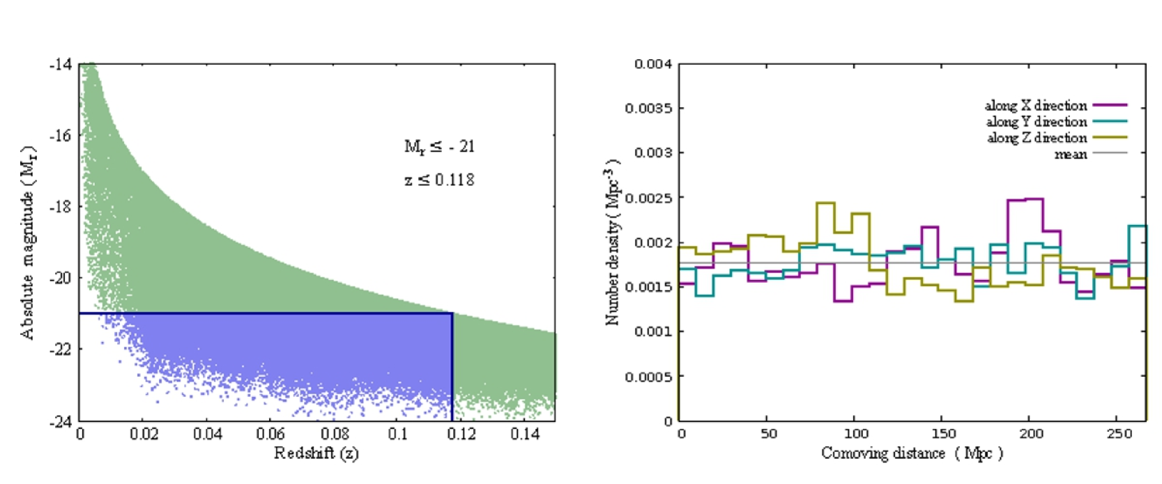
Figure 1: The definition of the volume-limited sample in the redshift-absolute magnitude plane is shown in the left panel. The right panel shows the variation of comoving number density inside the SDSS data cube along the three co-ordinate axes. The densities are evaluated using slices of thickness of $10\,{{\,\rm Mpc}}$.

Identifying the different morphological components of the cosmic web and analyzing these clustering patterns is a challenging task. Various statistical tools are developed for this purpose. Some of the measures are the void probability function (White, 1979), percolation analysis (Shandarin & Zeldovich, 1983), minimal spanning tree (Barrow, Bhavsar, & Sonoda, 1985), genus curve (Gott, Melott, & Dickinson, 1986), Minkowski functionals (Mecke, Buchert, & Wagner, 1994), multiscale morphology filter (Aragón-Calvo et al., 2007), skeleton (Novikov, Colombi, & Doré, 2006), spine (Aragón-Calvo et al., 2010) and the local dimension (Sarkar & Bharadwaj, 2009). The Minkowski functionals provide direct information on the geometry and topology of the galaxy distribution. The ratio of Minkowski functionals are used to construct Shapefinders (Sahni, Sathyaprakash, & Shandarin, 1998) that can describe the morphology of the large scale structures.

The filaments and the sheets are anisotropic structures with a great variety of shapes and sizes. It is generally difficult to define these structures and determine their size due to their structural variety and complexity. Some earlier works quantify the statistically significant length scale of filaments in the SDSS Main Galaxy sample (Bharadwaj, Bhavsar, & Sheth, 2004; Pandey & Bharadwaj, 2005; Pandey, 2010) and the Luminous Red Galaxy (LRG) sample (Pandey et al., 2011). The results show that the filaments are statistically significant up to $80{\,h^{-1}\,{\rm Mpc}}$ in the SDSS Main Galaxy distribution and $110{\,h^{-1}\,{\rm Mpc}}$ in the LRG distribution. These studies are based on the analysis of the two-dimensional projections of the three-dimensional galaxy distribution. The projection effects in such samples are expected to introduce spurious patterns. Some of the larger filaments in such sample may arise due to the projection of multiple filaments and sheets. Further, the sheet-like structures can not be studied reliably in such projected galaxy samples. Keeping these in mind, we plan to analyze the three-dimensional galaxy distribution from the SDSS to study the size of the longest filaments and the largest sheets in the cosmic web. It would determine the physical scale up to which the large-scale structures are coherent in a statistically significant way.

Sheth et al. (2003) develop the SURFGEN code to quantify the geometry and topology of the large-scale structures in the cosmic web. The method is used to study the morphology of the large-scale structures in simulations (Shandarin, Sheth, & Sahni, 2004) and mock galaxy catalogues (Sheth, 2004). The SURFGEN employs the ‘Marching Cube’ (Lorenson & Cliner, 1987) algorithm for triangulation and surface modelling. An advanced version of SURFGEN is developed by Bag et al. (2018) and named SURFGEN2. SURFGEN2 triangulates the surfaces by using the ‘Marching Cube 33’ (Chernyaev, 1995) algorithm. SURFGEN2 determines the Minkowski functionals and the Shapefinders for each identified structure. We plan to use SURFGEN2 to measure the filamentarity and planarity of the large-scale structures in three-dimension and assess their significance using a statistical technique ‘Shuffle’ (Bhavsar & Ling, 1988).

A brief outline of the paper follows. In section 2, we describe the data followed by the method of analysis in section 3. We present the results in section 4 and conclusions in section 5.

Throughout the paper, we use the $\Lambda$CDM cosmological model with $\Omega_{m0}=0.315$, $\Omega_{\Lambda 0}=0.685$ and $h=0.674$ (Planck Collaboration et al., 2018) for conversion of redshift to comoving distance.

2 DATA

2.1 SDSS DR17 data

We use data from the seventeenth data release (DR17) of the Sloan Digital Sky Survey (SDSS) for the present analysis. The SDSS is the largest redshift survey to date. It is a multi-band imaging and spectroscopic redshift survey that uses a 2.5 m telescope at Apache Point Observatory in New Mexico. A technical description of the SDSS telescope is provided in Gunn et al. (2006) and a technical summary of the survey can be found in York et al. (2000). The SDSS photometric camera is described in Gunn et al. (1998) and the selection criteria for the SDSS Main Galaxy sample is discussed in Strauss et al. (2002).

The SDSS, in its fourth phase, has mapped over 14 thousand square degrees of the sky, targeting about 500 million unique and primary sources, including over 200 million galaxies. For this study, we extract data from the seventeenth data release (DR17) (Abdurro’uf et al., 2022) of the SDSS. A structured query is run in the SDSS CasJobs to extract the required data.

We set the $scienceprimary$ flag to unity to ensure that only the targets with the best spectrum are chosen. The $zWarning$ flag is set to zero to select only the galaxies with a reliable redshift. A nearly uniform region is chosen within the right ascension and declination ranges $130^{\circ}\leq\alpha\leq 230^{\circ}$ and $0^{\circ}\leq\delta\leq 62^{\circ}$ respectively. We prepare a magnitude limited sample with the extinction corrected r-band apparent Petrosian magnitude $<17.77$ and $k$-corrected r-band Petrosian absolute magnitude limit $M_{r}\leq-21$ within the redshift range $0.01\leq z\leq 0.118$. The sample contains a total $113294$ galaxies. The definition of our volume-limited sample is shown in the left panel of Figure 1. The resulting sample has a radial extent of $507.85\,{{\,\rm Mpc}}$ and it covers a total volume of $6.73\times 10^{7}{{\,\rm Mpc}}^{3}$ with a mean number density of $1.68\times 10^{-3}{{\,\rm Mpc}}^{-3}$.

We finally carve out a cubic region from the volume-limited sample for our analysis. We consider the largest cube that can be extracted from the volume-limited sample. It provides us with a total $33648$ galaxies distributed within a cubic region of side $267{{\,\rm Mpc}}$. We show the variation of the comoving number density in this cubic region along three co-ordinates axes in the right panel of Figure 1.

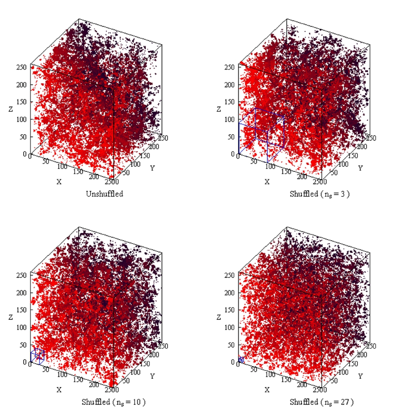
Figure 2: The top left panel shows the distribution of galaxies in the SDSS data cube. The other panels show one realization of the shuffled datasets for different $n_{s}$ values as mentioned in each panel. A shuffling unit corresponding to each $n_{s}$ value is shown (in blue) at the corner of the respective shuffled data cube.

3 METHOD OF ANALYSIS

3.1 Shuffle

We subdivide the original data cube of side $267\,{{\,\rm Mpc}}$ into $N_{c}=N_{s}^{3}$ smaller sub-cubes of size $l_{s}\,{{\,\rm Mpc}}$. The sub-cubes are rotated around any of the three axes by a random angle which is integral multiple of $90^{\circ}$. The axes of rotations are also decided randomly. The spatial positions of the rotated subcubes are then randomly interchanged. We repeat the random rotation followed by swapping for a total $100\times N_{c}$ times to generate a shuffled version (Bhavsar & Ling, 1988) of the original galaxy distribution within the SDSS data cube. We label this procedure as ‘shuffling’ and term $l_{s}$ as the ‘shuffling scale’. The shuffling of the original data is carried out for five different values of $n_{s}$. We choose the following values of $n_{s}$: $2,\,3,\,5,\,10,\,27$ that correspond to shuffling length of $133.5\,{{\,\rm Mpc}},\,89\,{{\,\rm Mpc}},\,53.4\,{{\,\rm Mpc}},\,26.7\,{{\,\rm Mpc}}$ and $9.89\,{{\,\rm Mpc}}$ respectively. The galaxy distributions in the original SDSS data cube and one shuffled realization for three different shuffling scales are shown in Figure 2.

3.2 Minkowski functionals

The Minkowski functionals (MFs) (Mecke, Buchert, & Wagner, 1994) can accurately describe the three-dimensional morphology of a closed two-dimensional surface. The four Minkowski functionals in three-dimensions are $-$ surface area ($S$), volume ($V$), integrated mean curvature ($C$), and integrated Gaussian curvature or Euler Characteristics ($\chi$). The first three MFs ($V,\,S$ and $C$) are geometric measures, while the fourth ($\chi$) is a topologically invariant measure. The surface area $S$ of the isodensity surface and the volume $V$ enclosed by it have the usual meaning. The Integrated mean curvature $C$ of the isodensity surface is defined as,

$$C=\tfrac{1}{2}\oint\big{(}\tfrac{1}{r_{1}}+\tfrac{1}{r_{2}}\big{)}\,dS$$ (1)

and the Euler characteristics $\chi$ of the isodensity surface is defined as,

$$\chi=\tfrac{1}{2\,\pi}\oint\big{(}\tfrac{1}{r_{1}\,r_{2}}\big{)}\,dS$$ (2)

where $r_{1}$ and $r_{2}$ are the principal radii of curvature at a point on the surface.

We estimate these MFs for the isodensity surfaces defined at different density thresholds. The distribution of the galaxies in the data cube is first converted to a density field on a rectangular grid of size $1\,{{\,\rm Mpc}}$ using the Cloud-in-Cell (CIC) scheme. The resulting discrete density field is then smoothed with a Gaussian filter of width $2\,{{\,\rm Mpc}}$. The set of isodensity surfaces is extracted from the smoothed density field at specific density thresholds ($\rho_{th}$). The isodensity surfaces bound the structures with density above the specific threshold. The individual structures are then identified with a grid version of the friend-of-friend (FOF) algorithm (Davis et al., 1985). We employ SURFGEN2 (Bag et al., 2018, 2019) to define the structures at each density threshold and calculate the associated MFs. For each structure recognized by FOF, SURFGEN2 constructs a closed triangulated surface using the Marching Cube 33 algorithm (Chernyaev, 1995). We determine the MFs on the triangulated surface using the following formula.

• $S=\sum_{i=1}^{N_{T}}S_{i}$, where $S_{i}$ is the area of the $i^{th}$ triangle and $N_{T}$ is the total number of triangles on the surface.
  

• $V=\sum_{i=1}^{N_{T}}S_{i}(\hat{n_{i}}.\vec{P_{i}})/3$, where $\hat{n_{i}}$ and $\vec{P_{i}}$ are the normal and centroid position vectors of $i^{th}$ triangle respectively.
  

• $C=\sum_{i,j}\epsilon\,l_{ij}\,\phi_{ij}$, where $l_{ij}$ and $\phi_{ij}$ are the common edge and angle between the normals of adjacent triangles, respectively. The local concavity and convexity of the surface is encoded in $\epsilon$ with values of $\epsilon=-1$ and $\epsilon=1$ respectively.
  

• $\chi=N_{T}-N_{E}+N_{V}$ where $N_{T},\,N_{E}$ and $N_{V}$ are respectively the total number of triangles, triangle-edges and triangle-vertices defining the isosurface.
  

3.3 Shapefinders

Using the MFs, Sahni, Sathyaprakash, & Shandarin (1998) introduces the Shapefinders to quantify the morphology of the large-scale structures in the galaxy distribution. They are the thickness $\mathcal{T}=3V/S$, breadth $\mathcal{B}=S/C$, and length $\mathcal{L}=C/4\pi$. All these measures have a dimension of length. These dimensional shapefinders and the Euler characteristics provide the typical size and topology of the structures. A set of dimensionless shapefinders, namely the filamentarity ($\mathcal{F}$) and planarity ($\mathcal{P}$), for each structures, are defined as follows:

$$\mathcal{F}=\frac{\mathcal{L}-\mathcal{B}}{\mathcal{L}+\mathcal{B}},\,\mathcal{P}=\frac{\mathcal{B}-\mathcal{T}}{\mathcal{B}+\mathcal{T}}$$ (3)

Here $\mathcal{F}=1,\,\mathcal{P}=0$ represents an ideal filament, whereas $\mathcal{F}=0,\,\mathcal{P}=1$ is for an ideal sheet. For the purpose of studying the general morphology of the galaxy distribution, we define average filamentarity and average planarity as the volume-weighted sum of the filamentarity and planarity of individual structures. They are defined as follows:

$$F_{a}=\frac{\sum_{i}V_{i}\mathcal{F}_{i}}{\sum_{i}V_{i}},\,\,P_{a}=\frac{\sum_{i}V_{i}\mathcal{P}_{i}}{\sum_{i}V_{i}}$$ (4)

where $V_{i}$ is the volume of $i^{th}$ structure identified by FOF for a given density threshold ($\rho_{th}$). The summation is across all such structures recognized by FOF for that $\rho_{th}$. Consequently, the structure with the highest volume contributes most to the $F_{a}$ and $P_{a}$. The largest structure grows in volume as the density threshold is lowered. The growth of the largest structure can be well captured by the Largest Cluster Statistic (LCS). The LCS is defined as the fraction of volume occupied by the largest structure. We calculate the LCS as,

$$LCS=\frac{V_{LS}}{\sum_{i}V_{i}},$$ (5)

where $V_{LS}$ is the volume of the largest structure.

We evaluate $F_{a}$, $P_{a}$ and the LCS for the original unshuffled SDSS data cube and five sets of shuffled data cubes at various density thresholds ($\delta\in[-0.8,12]$). Each shuffled set consists of ten realizations that are used to estimate the mean and $1\sigma$ errorbars for our measurements.

We quantitatively compare the average filamentarity and average planarity in the actual data to that with the shuffled datasets in the bottom right panel of Figure 3. We calculate the means $\bar{F_{a}}[{\it{Shuffled}}]$, $\bar{P_{a}}[{\it{Shuffled}}]$ and the variances $(\Delta F_{a}[{\it{Shuffled}}])^{2}$, $(\Delta P_{a}[{\it{Shuffled}}])^{2}$ for the average filamentarity and average planarity at each $\delta_{th}$ using 10 realizations for each shuffling scale. We quantify the difference between the average filamentarity of the actual data and the shuffled data using the $\chi^{2}$ per degree of freedom as,

$$\frac{\chi^{2}}{\nu}=\frac{1}{N_{p}-1}\sum_{i=1}^{N_{p}}\frac{(F_{a}[{\it{Actual}}]-\bar{F_{a}}[{\it{Shuffled}}])_{i}^{2}}{(\Delta F_{a}[{\it{Shuffled}}])_{i}^{2}}$$ (6)

where $N_{p}$ is the total number of density threshold used in the analysis. We also estimate the $\chi^{2}$ per degree of freedom for the average planarity as a function of shuffling scale in a similar manner.

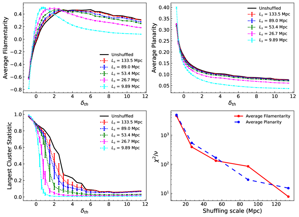
Figure 3: The top left, top right and bottom left panels of this figure respectively show the average filamentarity, average planarity and largest cluster statistic in the original unshuffled data and its shuffled versions as a function of the density threshold. The largest cluster statistic is the fractional volume occupied by the largest cluster. The shuffling scale associated with each shuffled version are indicated in each panel. The $1\sigma$ error bars at each data point are obtained from 10 different realizations for each shuffling scale. The errorbars for the average filamentarity and planarity are noticeably small. We quantify the difference between the original and the shuffled data as a function of the shuffling scale in the bottom right panel.

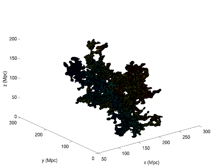
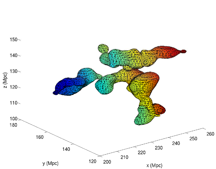
Figure 4: The left panel shows the largest structure identified from the smooth density field of the SDSS galaxy distribution at a density threshold of $\delta_{th}=3$ before the onset of percolation. The right panel shows the largest structure in one of the shuffled realizations with a shuffling scale of $9.89\,{{\,\rm Mpc}}$. The largest structure in the shuffled data is also identified at the same density threshold. It may be noted that the two panels cover different ranges of length scales. The relatively smaller size of the largest structure in the shuffled data at the same density threshold is evident in this figure. The figure clearly shows that the largest structure in the original data poses a higher degree of filamentarity and connectivity compared to the same in the shuffled data.

4 RESULTS

We analyze the SDSS galaxy distribution within the cubic region and its different shuffled versions using SURFGEN2. The results of our analysis are shown in different panels of Figure 3.

We show the average filamentarity ($F_{a}$) in the original unshuffled galaxy distribution as a function of the threshold density contrast ($\delta_{th}$) in the top left panel of Figure 3. The average filamentarity in the different shuffled versions of the original galaxy distribution are also shown together in the same panel. The $1\sigma$ errorbars shown at each data point for the shuffled data are obtained from 10 realizations for each shuffling scale. We find that for both the unshuffled and the shuffled data, the average filamentarity in the galaxy distribution slowly increases with the decreasing density threshold and eventually reaches a maximum. It then decays rapidly for a further decrease in the density threshold. For the original unshuffled data, the average filmentarity reaches a maximum at $\delta_{th}\sim 3$. The average filamentarity drops to subzero values at $\delta_{th}<0.1$.

Lowering the density threshold interconnects the individual structures, producing even larger structures. The filamentarity of the galaxy distribution keeps increasing until the percolation threshold is reached. At percolation, the individual structures rapidly merge into a connected structure spanning the entire volume. The density threshold corresponding to this rapid transition is termed the percolation threshold. The galaxy distribution assumes a sponge-like topology after the onset of percolation, where the large-scale structures interconnect into a giant network surrounded by immense voids. After the percolation transition, the network becomes thicker, and the voids turn rounder when the density threshold is lowered further. The large near spherical voids surrounded by the filaments introduce considerable negative curvature in the system. This negative curvature is responsible for the sizeable negative filamentarity at a very low-density threshold.

The average filamentarity in the shuffled data is significantly lower than that in the unshuffled data at $\delta_{th}>3$. It indicates that the shuffled galaxy distributions are less fiamentary than the original unshuffled data. The shuffled data with the smallest shuffling scale shows the largest drop in the average filamentarity. The average filamentarity in the shuffled data at each density threshold beyond $\delta_{th}=3$ increases with the increasing shuffling scale which clearly shows that the shuffling procedure destroys many filaments in the galaxy distribution. The shuffling destroys the filaments when the shuffling scale is smaller than the size of the filaments in the data. At $\delta_{th}<3$, we see a reversal in the trend. The shuffled data have a higher average filamentarity than the actual data simply because of the shift of the percolation threshold in the shuffled data to lower density. It may be noted that the average filamentarity peaks at a lower density threshold for the shuffled datasets.

We show the average planarity ($P_{a}$) in the original unshuffled galaxy distribution and its shuffled versions as a function of the density threshold in the top right panel of Figure 3. We find that the average planarity steadily increases for both the unshuffled and shuffled data as we lower the density threshold. After the percolation transition, the filaments only grow thicker with decreasing density threshold. Consequently, the large-scale structures assume an increasingly planar morphology at a lower density threshold.

While comparing the average planarity of the shuffled data with that from the original unshuffled data, we note that the average planarity decreases at each density threshold with increasing shuffling scale. The shuffled data with the smallest shuffling scale show the most significant drop in the average planarity. These clearly show that shuffling the data destroys the sheet-like structures in the galaxy distribution. The differences between the average planarity of the original and the shuffled datasets are more visible if we use a logarithmic scale for the average planarity. Here we have plotted the average planarity in a linear scale.

In other words, the difference between the average filamentarity or the average planarity in the unshuffled and the shuffled data decreases with the increasing shuffling scale. It can be understood as follows. The original data may have coherent filaments and sheets up to specific length scales. Shuffling the data would destroy all the filaments and sheets spanning beyond the shuffling scale. However, the filaments and sheets smaller than the shuffling length scale would survive and remain nearly intact. If the most extended filaments or the most extensive sheets are shorter than the shuffling length then the average filamentarity or the average planarity in the shuffled data would not show any significant changes from that in the original data. Shuffling the data on a larger scale allows more filaments and sheets to survive the shuffling process. At a given shuffling scale, the average filamentarity or the average planarity in the original data would be larger than in the shuffled data only if the original data have more filaments or sheets spanning beyond the shuffling length, than that expected from chance alignments. When the average filamentarity or the average planarity in the original data are within the $1\sigma$ errorbars of that for the shuffled data then one can infer that the maximum size of the filaments or sheets must be smaller than the associated shuffling scale. This would only occur when the longest filaments or the largest sheets are shorter than the associated shuffling scale. Larger filaments or sheets may still exist in the galaxy distribution but they are the product of pure chance alignments.

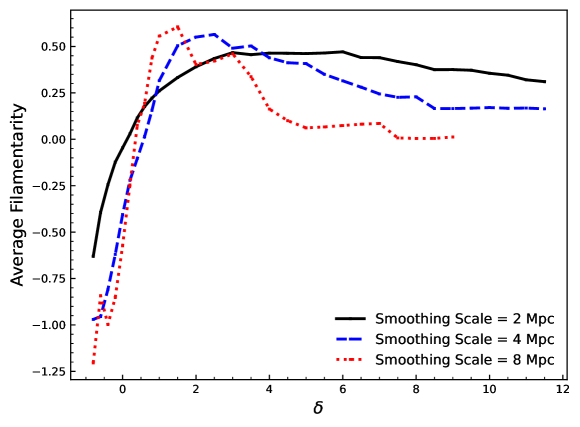
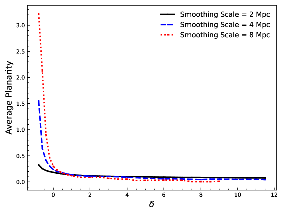
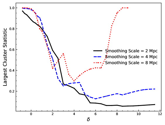
Figure 5: The three panels of this figure show the average filamentarity, average planarity and the largest cluster statistic in the original SDSS data as a function of density threshold for three different smoothing lengths.

The bottom right panel of Figure 3 shows the chi-square per degree of freedom for the average filamentarity and the average planarity, as a function of the shuffling scale. The chi-square per degree of freedom is very large ($\sim 4.5\times 10^{3}$) at the smallest shuffling scale ($9.89\,{{\,\rm Mpc}}$) for both the average filamentarity and average planarity. It suggests that the filaments and sheets are highly significant at this length scale. In both cases, the $\chi^{2}/\nu$ gradually decreases with the increasing shuffling scale. We note that it decreases to a value of $\sim 8$ for the average filamentarity and $\sim 15$ for the average planarity at the shuffling scale of $133.5\,{{\,\rm Mpc}}$. So the average filamentarity and the average planarity in the shuffled data differ from the actual data in a statistically significant way, even at the largest shuffling scale of $133.5\,{{\,\rm Mpc}}$. It implies that the filaments and sheets in the galaxy distribution are statistically significant up to the largest length scale probed in this analysis. Ideally, a $\frac{\chi^{2}}{\nu}\sim 1$ would indicate the filaments or sheets span up to the same length scales in the original and shuffled data and no structures are destroyed by the shuffling procedure. Unfortunately, we can not probe the length scales beyond $133.5\,{{\,\rm Mpc}}$ with the existing data. Shuffling the data on somewhat larger scales ($150-200\,{{\,\rm Mpc}}$) would most likely eliminate all the differences observed between the actual and the shuffled data. A larger value of the chi-square per degree of freedom for the average planarity compared to the average filamentarity at the largest shuffling scale indicates that the largest sheets may extend to somewhat larger length scales than the longest filaments.

The average filamentarity and planarity are mostly contributed by the structures with larger volumes. Naturally, the largest structure at any given density threshold contributes more to these statistics. We show the Largest Cluster Statistic (LCS) as a function of the density threshold for the original and shuffled data in the bottom left panel of Figure 3. The LCS quantifies the fraction of volume occupied by the largest structure and shows the growth of the largest structure with decreasing density threshold. A faster growth of the LCS indicates greater connectivity of the large-scale structures in the galaxy distribution. The bottom left panel of Figure 3 shows that the LCS grows slowly in the original SDSS data as the density threshold is lowered. The LCS in the SDSS data shows a sudden jump from $0.25$ to $0.75$ when the density threshold ($\delta_{th}$) is decreased from 3 to 2. The sudden jump in the LCS corresponds to the percolation transition. The LCS in all the shuffled data sets are clearly smaller than the actual data for $\delta_{th}>0$. The jump in the LCS occurs at a smaller density threshold for the shuffled data, indicating a shift in their percolation threshold to the lower densities. The LCS in the shuffled data decreases at each density threshold with the decreasing shuffling scale. We note that for the smallest shuffling scale, the LCS stays $\sim 0.02-0.05$ up to $\delta_{th}\sim 1$ and then suddenly jumps to $0.8$ at $\delta_{th}\sim 0.5$. It clearly shows that shuffling the data decreases the connectivity of the galaxy distribution by destroying large-scale patterns like sheets and filaments. The results shown in this panel also assert that shuffling the data on a scale of $133.5\,{{\,\rm Mpc}}$ diminish the connectivity in the galaxy distribution in a statistically significant way. It is consistent with the results obtained from the analysis of the average filamentarity and planarity.

We show the largest structure before the onset of percolation in the original data at $\delta_{th}=3$ in the left panel of Figure 4. The largest structure identified from one of the shuffled realizations with shuffling scale $9.89\,{{\,\rm Mpc}}$ is shown for comparison in the right panel of Figure 4. The largest structure in the shuffled data shown in this panel is also identified at $\delta_{th}=3$. It may be noted that the two panels cover different ranges of length scales, and the largest structure in the shuffled data is noticeably smaller compared to the original data at the same density threshold. The largest structure in the shuffled data is a simply connected object, whereas the one in the original data is a multiply connected complex object with a higher degree of filamentarity and connectivity.

The results for the SDSS data in Figure 3 hint a critical density threshold at $\delta\sim 3$ below which most of the individual structures interconnect to become one single network-like structure spanning the entire volume. This corresponds to the percolating density threshold. We test if this threshold depends on the smoothing length chosen for the analysis. We compare the average filamenarity, average planarity and the largest cluster statistic for 3 different smoothing lengths in Figure 5. We find that the percolating density threshold is sensitive to the smoothing length. We analyze the SDSS data with smoothing lengths of 2 Mpc, 4 Mpc and 8 Mpc and note that the percolating density thresholds decreases with the increasing smoothing length. The results for different smoothing lengths are qualitatively similar. We notice that for the smoothing length of 8 Mpc, LCS shows a strikingly different behaviour where it initially decreases and then increases with the decreasing density threshold. A higher smoothing would lead to lesser number of high density regions. So there will be very few structures at higher density thresholds. The LCS would be very high ($\sim 1$) when the largest among these few structures is significantly larger than the rest. The LCS initially decreases with the increase in the available number of structures as the density threshold is lowered. However, these structures would then start connecting into a network eventually reaching percolation at some lower density threshold.

The mean intergalactic separation for our sample is $\sim 8$ Mpc whereas we have chosen a smoothing length of 2 Mpc. The choice of a larger smoothing length affects the measurements at the higher density regions as discussed earlier. On the other hand, a smoothing length smaller than the mean intergalactic separation would lead to a greater abundance of the low-density regions that may affect some of our results at lower density. Keeping this possibility in mind, we also repeat our chi-square analysis considering only the results above $\delta_{th}>3$. We find that our conclusions remain unchanged.

5 CONCLUSIONS

Large-scale structures like sheets and filaments are striking visual patterns observed in galaxy distribution. The statistical significance of these large-scale clustering patterns is difficult to judge by visual inspections or automated identification schemes. The sheets and filaments are anisotropic structures that introduce significant inhomogeneity and anisotropy in the galaxy distribution. They may vary widely in size and shape (Pimbblet, Drinkwater, & Hawkrigg, 2004; Colberg, Krughoff, & Connolly, 2005). However, their large-scale distribution is expected to be uniform, provided our Universe conforms to the cosmological principle. Any such uniformity can only be achieved beyond the length-scale of the largest patterns present in the galaxy distribution. In this context, the maximum size of these large-scale structures may be treated as a lower limit for the scale of homogeneity.

In this work, we attempt to quantify the maximum extent of the sheets and filaments in the three-dimensional galaxy distribution for the first time. Some analyses have been carried out for the filaments in some earlier works (Bharadwaj, Bhavsar, & Sheth, 2004; Pandey & Bharadwaj, 2005; Pandey et al., 2011) using the projected galaxy distributions on two-dimension. These analyses are prone to projection effects where larger filaments can arise due to the projection of multiple sheets and filaments.

We use the SDSS data to construct a volume-limited galaxy sample within a cubic region and quantify the largest cluster statistic, average filamentarity and average planarity as a function of the density threshold. The largest cluster statistic quantifies the connectivity in the galaxy distribution and exhibits a sudden jump at the percolation threshold. The average filamentarity reaches a maximum at the percolation threshold and decreases at a lower density. The average planarity, on the other hand, increases with the decreasing density threshold. These statistics provide a combined picture where the galaxy distribution becomes more filamentary and planar with decreasing density threshold. The filaments and sheets interconnect to produce larger structures as the density threshold is lowered. Finally, all the individual structures merge into a giant sponge-like network spanning the entire volume.

The morphology of the large-scale structures is well described by the Shapefinders at and above the percolation threshold. We compare the average filamentarity and planarity in the original galaxy distribution to those from the shuffled data and find a statistically significant reduction in their values at all the density thresholds above $3$. The difference between the original and the shuffled data reduces with the increasing shuffling scale at each density threshold. We quantify the differences using the chi-square per degree of freedom and find that both the filaments and sheets remain statistically significant up to the length scale of $133.5\,{{\,\rm Mpc}}$. Our analysis is limited by the physical size of the SDSS data cube. $133.5$ Mpc is the highest shuffling scale employed in the present work. So the present analysis suggests that the filaments and the sheets extend up to $\sim 130\,{{\,\rm Mpc}}$. They may even extend to somewhat larger length scales not captured in our analysis. We do not attempt to extrapolate our results to arrive at any definite conclusion. The fact that the differences are more significant for sheets than the filaments at the largest shuffling scale implies that the sheets may extend to larger lengths than the filaments. It is interesting to note that the result of this analysis is consistent with the measured scale of homogeneity and isotropy from different datasets.

We carry out our analysis in the redshift space. It is worthwhile to mention here that the redshift space distortions (RSD) may have significant impact on the size of the structures in our analysis. It is well known that the structures in the real-space and redshift-space have different power spectra, correlation functions, and pdfs (Kaiser, 1987; Hamilton, 1992; Hui, Kofman, & Shandarin, 2000). Besides, the size of the structures can be considerably larger in redshift space compared to the original structures in real space (Praton, Melott, & McKee, 1997; Melott et al., 1998). Shandarin (2009) show that the size of the structures in redshift space are significantly larger in the transverse direction than in the line of sight direction. Thus RSD can play a substantial role in the apparent detection of structures like ‘great walls’. This implies that some of the large-scale structures in our dataset may not exist in real-space and arises due to the RSD. In a strict sense, our results are valid in redshift space. The geometry of the survey boundary and the shot noise can also introduce some systematic effects on the size of the structures. In future, we plan to use large-volume cosmological simulations to quantify the effects of RSD, survey boundaries and shot noise on the maximum extent of the large-scale structures.

We will be able to measure the maximum size of the sheets and filaments in a more conclusive manner with the upcoming EUCLID survey (Euclid Collaboration et al., 2022). The EUCLID is expected to provide $\sim 30$ million spectroscopic redshifts over a sky area of $15000$ square degrees and up to a redshift of $z\sim 2$.

Finally, we conclude that the sheets and filaments in the 3D galaxy distribution are statistically significant up to $\sim 130\,{{\,\rm Mpc}}$. The maximum size of the filaments and sheets can be somewhat larger but should be pretty close to this length scale. We expect to determine these length scales using our method to deeper and larger galaxy surveys in future.

6 ACKNOWLEDGEMENT

We sincerely thank an anonymous reviewer for the valuable comments and suggestions that helped us to improve the draft. The authors thank the SDSS team for making the data publicly available. PS acknowledges discussions with Varun Sahni and Satadru Bag during the development of SURFGEN2. BP would like to acknowledge financial support from the SERB, DST, Government of India through the project CRG/2019/001110. BP would also like to acknowledge IUCAA, Pune for providing support through associateship programme. SS acknowledges IISER Tirupati for support through a postdoctoral fellowship.

Funding for the SDSS and SDSS-II has been provided by the Alfred P. Sloan Foundation, the Participating Institutions, the National Science Foundation, the U.S. Department of Energy, the National Aeronautics and Space Administration, the Japanese Monbukagakusho, the Max Planck Society, and the Higher Education Funding Council for England. The SDSS website is http://www.sdss.org/.

The SDSS is managed by the Astrophysical Research Consortium for the Participating Institutions. The Participating Institutions are the American Museum of Natural History, Astrophysical Institute Potsdam, University of Basel, University of Cambridge, Case Western Reserve University, University of Chicago, Drexel University, Fermilab, the Institute for Advanced Study, the Japan Participation Group, Johns Hopkins University, the Joint Institute for Nuclear Astrophysics, the Kavli Institute for Particle Astrophysics and Cosmology, the Korean Scientist Group, the Chinese Academy of Sciences (LAMOST), Los Alamos National Laboratory, the Max-Planck-Institute for Astronomy (MPIA), the Max-Planck-Institute for Astrophysics (MPA), New Mexico State University, Ohio State University, University of Pittsburgh, University of Portsmouth, Princeton University, the United States Naval Observatory, and the University of Washington.

7 DATA AVAILABILITY

The data underlying this article are publicly available at https://skyserver.sdss.org/casjobs/.

References

- Abdurro’uf et al. (2022) Abdurro’uf, Accetta K., Aerts C., Silva Aguirre V., Ahumada R., Ajgaonkar N., Filiz Ak N., et al., 2022, ApJS, 259, 35
- Alonso et al. (2015) Alonso D., Salvador A. I., Sánchez F. J., Bilicki M., García-Bellido J., Sánchez E., 2015, MNRAS, 449, 670
- Appleby et al. (2022) Appleby S., Park C., Pranav P., Hong S. E., Hwang H. S., Kim J., Buchert T., 2022, ApJ, 928, 108
- Aragón-Calvo et al. (2007) Aragón-Calvo M. A., Jones B. J. T., van de Weygaert R., van der Hulst J. M., 2007, A&A, 474, 315
- Aragón-Calvo et al. (2010) Aragón-Calvo M. A., Platen E., van de Weygaert R., Szalay A. S., 2010, ApJ, 723, 364
- Avila et al. (2019) Avila F., Novaes C. P., Bernui A., de Carvalho E., Nogueira-Cavalcante J. P., 2019, MNRAS, 488, 1481
- Bag et al. (2018) Bag S., Mondal R., Sarkar P., Bharadwaj S., Sahni V., 2018, MNRAS, 477, 1984
- Bag et al. (2019) Bag S., Mondal R., Sarkar P., Bharadwaj S., Choudhury T. R., Sahni V., 2019, MNRAS, 485, 2235
- Bagchi et al. (2017) Bagchi J., Sankhyayan S., Sarkar P., Raychaudhury S., Jacob J., Dabhade P., 2017, ApJ, 844, 25
- Barrow, Bhavsar, & Sonoda (1985) Barrow J. D., Bhavsar S. P., Sonoda D. H., 1985, MNRAS, 216, 17
- Bharadwaj et al. (1999) Bharadwaj, S., Gupta, A. K., & Seshadri, T. R. 1999, A&A, 351, 405
- Bhavsar & Ling (1988) Bhavsar, S. P. & Ling, E. N. 1988, ApJ Letters, 331, L63
- Bond, Kofman & Pogosyan (1996) Bond, J. R., Kofman, L., & Pogosyan, D., 1996, Nature, 380, 603
- Borgani (1995) Borgani, S. 1995, Physics Reports, 251, 1
- Bharadwaj, Bhavsar, & Sheth (2004) Bharadwaj S., Bhavsar S. P., Sheth J. V., 2004, ApJ, 606, 25
- Blake & Wall (2002) Blake, C., & Wall, J. 2002, Nature, 416, 150
- Bengaly et al. (2017) Bengaly, C. A. P., Bernui, A., Ferreira, I. S., & Alcaniz, J. S. 2017, MNRAS, 466, 2799
- Chernyaev (1995) Chernyaev E. V., 1995, Technical Report CERN-CN/95-17
- Clowes et al. (2013) Clowes R. G., Harris K. A., Raghunathan S., Campusano L. E., Söchting I. K., Graham M. J., 2013, MNRAS, 429, 2910
- Colless et al. (2001) Colless M., Dalton G., Maddox S., Sutherland W., Norberg P., Cole S., Bland-Hawthorn J., et al., 2001, MNRAS, 328, 1039
- Colberg, Krughoff, & Connolly (2005) Colberg J. M., Krughoff K. S., Connolly A. J., 2005, MNRAS, 359, 272
- Colin et al. (2019) Colin J., Mohayaee R., Rameez M., Sarkar S., 2019, A&A, 631, L13
- Davis et al. (1985) Davis M., Efstathiou G., Frenk C. S., White S. D. M., 1985, ApJ, 292, 371
- Einasto, Joeveer, & Saar (1980) Einasto J., Joeveer M., Saar E., 1980, MNRAS, 193, 353
- Einasto et al. (1984) Einasto J., Klypin A. A., Saar E., Shandarin S. F., 1984, MNRAS, 206, 529
- Einasto et al. (2014) Einasto M., Lietzen H., Tempel E., Gramann M., Liivamägi L. J., Einasto J., 2014, A&A, 562, A87
- Euclid Collaboration et al. (2022) Euclid Collaboration, Scaramella R., Amiaux J., Mellier Y., Burigana C., Carvalho C. S., Cuillandre J.-C., et al., 2022, A&A, 662, A112
- Fixsen et al. (1996) Fixsen, D. J., Cheng, E. S., Gales, J. M., et al. 1996, ApJ, 473, 576
- Gibelyou & Huterer (2012) Gibelyou, C., & Huterer, D. 2012, MNRAS, 427, 1994
- Gonçalves et al. (2021) Gonçalves R. S., Carvalho G. C., Andrade U., Bengaly C. A. P., Carvalho J. C., Alcaniz J., 2021, JCAP, 2021, 029
- Gott, Melott, & Dickinson (1986) Gott J. R., Melott A. L., Dickinson M., 1986, ApJ, 306, 341
- Gott et al. (2005) Gott, J. R., III, Jurić, M., Schlegel, D., et al. 2005, ApJ, 624, 463
- Gregory & Thompson (1978) Gregory S. A., Thompson L. A., 1978, ApJ, 222, 784
- Gunn et al. (2006) Gunn, J. E., Siegmund, W. A., Mannery, E. J., Owen, R. E., Hull, C. L., Leger, R. F., Carey, L. N., et al., 2006, AJ, 131, 2332
- Gunn et al. (1998) Gunn, J. E., Carr, M., Rockosi, C., Sekiguchi, M., Berry, K., Elms, B.,Has, E. de, et al., 1998, AJ, 116, 3040
- Gupta & Saini (2010) Gupta, S., & Saini, T. D. 2010, MNRAS, 407, 651
- Guzzo (1997) Guzzo L., 1997, New Astronomy, 2, 517
- Hamilton (1992) Hamilton A. J. S., 1992, ApJL, 385, L5
- Hogg et al. (2005) Hogg, D. W., Eisenstein, D. J., Blanton, M. R., Bahcall, N. A., Brinkmann, J., Gunn, J. E., & Schneider, D. P. 2005, ApJ, 624, 54
- Hui, Kofman, & Shandarin (2000) Hui L., Kofman L., Shandarin S. F., 2000, ApJ, 537, 12
- Joeveer & Einasto (1978) Joeveer M., Einasto J., 1978, IAUS, 79, 241
- Kaiser (1987) Kaiser N., 1987, MNRAS, 227, 1
- Keenan, Barger, & Cowie (2013) Keenan R. C., Barger A. J., Cowie L. L., 2013, ApJ, 775, 62
- Lietzen et al. (2016) Lietzen H., Tempel E., Liivamägi L. J., Montero-Dorta A., Einasto M., Streblyanska A., Maraston C., et al., 2016, A&A, 588, L4
- Lopez, Clowes, & Williger (2022) Lopez A. M., Clowes R. G., Williger G. M., 2022, arXiv:2201.06875
- Lorenson & Cliner (1987) Lorenson, W.E. & Cline, H.E., 1987, Computer Graphics, 21, 163
- Marinoni et al. (2012) Marinoni, C., Bel, J., & Buzzi, A. 2012, JCAP, 10, 036
- Martinez & Coles (1994) Martinez, V. J., & Coles, P. 1994, ApJ, 437, 550
- Mecke, Buchert, & Wagner (1994) Mecke K. R., Buchert T., Wagner H., 1994, A&A, 288, 697
- Melott et al. (1998) Melott A. L., Coles P., Feldman H. A., Wilhite B., 1998, ApJL, 496, L85
- Novikov, Colombi, & Doré (2006) Novikov D., Colombi S., Doré O., 2006, MNRAS, 366, 1201
- Pan & Coles (2000) Pan, J., & Coles, P. 2000, MNRAS, 318, L51
- Pandey & Bharadwaj (2005) Pandey B., Bharadwaj S., 2005, MNRAS, 357, 1068
- Pandey (2010) Pandey B., 2010, MNRAS, 401, 2687
- Pandey et al. (2011) Pandey B., Kulkarni G., Bharadwaj S., Souradeep T., 2011, MNRAS, 411, 332
- Pandey & Sarkar (2015) Pandey B., Sarkar S., 2015, MNRAS, 454, 2647
- Pandey & Sarkar (2016) Pandey B., Sarkar S., 2016, MNRAS, 460, 1519
- Pandey (2017) Pandey, B. 2017, MNRAS, 468, 1953
- Pandey & Sarkar (2021) Pandey B., Sarkar S., 2021, JCAP, 2021, 019
- Penzias & Wilson (1965) Penzias, A. A., & Wilson, R. W. 1965, ApJ, 142, 419
- Pimbblet, Drinkwater, & Hawkrigg (2004) Pimbblet K. A., Drinkwater M. J., Hawkrigg M. C., 2004, MNRAS, 354, L61
- Planck Collaboration et al. (2018) Planck Collaboration, Aghanim, N., Akrami, Y., Ashdown, M., Aumont, J., Baccigalupi, C., Ballardini, M., et al., 2018, A&A, 641, A6
- Porter & Raychaudhury (2007) Porter S. C., Raychaudhury S., 2007, MNRAS, 375, 1409
- Praton, Melott, & McKee (1997) Praton E. A., Melott A. L., McKee M. Q., 1997, ApJL, 479, L15
- Sahni, Sathyaprakash, & Shandarin (1998) Sahni V., Sathyaprakash B. S., Shandarin S. F., 1998, ApJL, 495, L5
- Sarkar et al. (2009) Sarkar, P., Yadav, J., Pandey, B., & Bharadwaj, S. 2009, MNRAS, 399, L128
- Sarkar & Bharadwaj (2009) Sarkar P., Bharadwaj S., 2009, MNRAS, 394, L66
- Sarkar & Pandey (2016) Sarkar S., Pandey B., 2016, MNRAS, 463, L12
- Sarkar & Pandey (2019) Sarkar S., Pandey B., 2019, MNRAS, 485, 4743
- Sarkar, Pandey, & Khatri (2019) Sarkar S., Pandey B., Khatri R., 2019, MNRAS, 483, 2453
- Scrimgeour et al. (2012) Scrimgeour, M. I., Davis, T., Blake, C., et al. 2012, MNRAS, 3412
- Scharf et al. (2000) Scharf, C. A., Jahoda, K., Treyer, M., et al. 2000, ApJ, 544, 49
- Secrest et al. (2021) Secrest N. J., von Hausegger S., Rameez M., Mohayaee R., Sarkar S., Colin J., 2021, ApJL, 908, L51
- Sheth et al. (2003) Sheth J. V., Sahni V., Shandarin S. F., Sathyaprakash B. S., 2003, MNRAS, 343, 22
- Sheth (2004) Sheth J. V., 2004, MNRAS, 354, 332
- Shandarin & Zeldovich (1983) Shandarin S. F., Zeldovich I. B., 1983, Comments on Astrophysics, 10, 33
- Shandarin, Sheth, & Sahni (2004) Shandarin S. F., Sheth J. V., Sahni V., 2004, MNRAS, 353, 162
- Shandarin (2009) Shandarin S. F., 2009, JCAP, 2009, 031
- Smoot et al. (1992) Smoot, G. F., Bennett, C. L., Kogut, A., et al. 1992, ApJ Letters, 396, L1
- Stoughton et al. (2002) Stoughton C., Lupton R. H., Bernardi M., Blanton M. R., Burles S., Castander F. J., Connolly A. J., et al., 2002, AJ, 123, 485
- Strauss et al. (2002) Strauss, M. A., Weinberg, D. H., Lupton, R. H., Narayanan, V. K., Annis, J., Bernardi, M., Blanton, M., et al., 2002, AJ, 124, 1810
- Tully et al. (2014) Tully R. B., Courtois H., Hoffman Y., Pomarède D., 2014, Nature, 513, 71
- White (1979) White S. D. M., 1979, MNRAS, 186, 145
- Wiegand, Buchert, & Ostermann (2014) Wiegand A., Buchert T., Ostermann M., 2014, MNRAS, 443, 241
- Wu et al. (1999) Wu, K. K. S., Lahav, O., & Rees, M. J. 1999, Nature, 397, 225
- Yadav et al. (2005) Yadav, J., Bharadwaj, S., Pandey, B., & Seshadri, T. R. 2005, MNRAS, 364, 601
- Yoon et al. (2014) Yoon, M., Huterer, D., Gibelyou, C., Kovács, A., & Szapudi, I. 2014, MNRAS, 445, L60
- York et al. (2000) York D. G., Adelman J., Anderson J. E., Anderson S. F., Annis J., Bahcall N. A., Bakken J. A., et al., 2000, AJ, 120, 1579
- Zeldovich & Shandarin (1982) Zeldovich I. B., Shandarin S. F., 1982, PAZh, 8, 131