myequation
|
|
(1) |
Persistence of an active asymmetric rigid Brownian particle in two dimensions
Abstract
We have studied the persistence probability of an active Brownian particle with shape asymmetry in two dimensions. The persistence probability is defined as the the probability of a stochastic variable that has not changed it’s sign in the fixed given time interval. We have investigated two cases- diffusion of a free active particle and that of harmonically trapped particle. In our earlier work, Ghosh et. al., Journal of Chemical Physics, 152,174901, (2020), we had shown that can be used to determine translational and the rotational diffusion constant of an asymetric shape particle. The method has the advantage that the measurement of the roational motion of the anisotropic particle is not required. In this paper, we extend the study to an active an-isotropic particle and show how the persistence probability of an anisotropic particle is modified in the presence of a propulsion velocity. Further, we validate our analytical expression against the measured persistence probability from the numerical simulations of single particle Langevin dynamics and test whether the method proposed in our earlier work can distinguish between an active and a passive anisotropic particle.
Appendix A Introduction
Persistence plays a very important role in describing a stochastic processes in nature, specifically the non-stationary dynamics of the system. The phenomenon of persistence is typically quantified through the persistence probability. For the last two decades,this has attracted quite significant attention in the scientific community. The persistence probability of a stochastic variable is the probability that the variable has not changed its sign up to time . In a wide range of non-equilibrium systems is found to decay algebraically with an exponent , , where -is a non-trivial exponent. As the temporal correlation of the non-Markovian stochastic process is highly non-local in behaviour, the exact calculation of persistence for even simple non-Markovian stochastic systems is often very difficult and exact analytical expression for exists for very few cases. In spite of this, analytical and or numerical results for the persistence probability and the exponent exists for systems such as Brownian motion and diffusion process1; 2; 3; 4; 5; 6; 7; 8; 9; 10, reaction-diffusion systems11; 12,dynamical systems 13, phase ordered kinetics14; 15; 16, fluctuating interfaces17; 18; 19; 20, critical dynamics21; 22, polymer dynamics23; 24, financial markets25; 26 and many more. Even experimental results exist for persistence exponent in one-dimensional Ising model27, diffusion process 28,fluctuating steps and interfaces29. For a more comprehensive review, we invite the readers to the review by Bray et. al. 30 and Majumdar 1.
The route to calculating of the persistence probability is through the non-stationary two-time correlation function. The Lamperti transformation converts the non-stationary correlator to a stationary process. For a Gaussian-Markovian stochastic process, the persistence probability can be directly calculated using Slepian’s theorem 31. In contrast, when the process is Non-Markovian, is evaluated either using the Independent Interval Approximation (IIA) when the density of zero crossings stays finite or a perturbative expansion.
In our earlier work we investigated the effect of shape asymmetry on the persistence probability of a Brownian particle.32 We explicitly showed that the measured persistence probability could estimate the translational and the rotational diffusion constants of an asymmetric shape particle. The method has the advantage that the measurement of the rotational motion of the anisotropic particle is not required. In this paper, we extend the study to an active anisotropic particle. Our main interest lies in how the persistence probability of an anisotropic particle is modified in the presence of a propulsion velocity and whether the method proposed in our earlier work can distinguish between an active and a passive anisotropic particle.
This article is organized as follows: In the Appendix B we have presented the results for the two-time correlation function for the position of a free active Brownian particle with shape asymmetry and along with that the survival probability has been calculated from the two-time correlation. In the Appendix C, we have carried out a perturbative expansion for the position of an anisotropic active Brownian particle trapped in a harmonic potential. The two-time correlation has been calculated using the perturbative expansion method. Finally persistence probability is constructed from the two-time correlation function.
Appendix B Active asymmetric particle in two dimensions
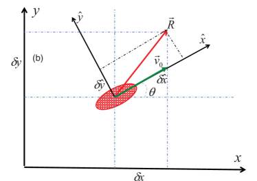
We consider an self propelled asymmetric particle with velocity in two dimensions with mobilities and along the longer and the shorter axes of the particle, respectively. We have fixed the body frame and directions as the long and the short axis, respectively. The particle has a single rotational mobility . The particle is immersed in a bath of temperature so that the translational diffusion coefficients along the two directions are given by and , and the rotational diffusion constant is . At a given time the particle can be described by the position vector of its center of mass and the angle between the axis of the lab-frame and the long axis of the particle. In this frame, the self-propulsion speed, which is taken along the long axis of the rod, is given by, , where is a unit vector along the long axis of the particle. In the body frame, the equations of motion for the center of mass of the particle take the form
| (2) |
Here and are the forces acting on the particle along the and axes(in the lab frame), respectively, and is the torque acting on the particle. The correlations of the thermal fluctuations in the body frame are given by
| (3) |
In the lab frame, the displacements are related to the body frame as
| (4) |
Using the transformation in Eq. 4, the corresponding equations in the lab frame is given by
| (5) |
The thermal fluctuations given in Eq. 4 are also transformed in the body frame. The correlations of the thermal fluctuations in the body frame are given by
| (6) |
and
| (7) |
Here and , and mobility tensor can be written as , when the form of is written as
B.1 Mean Square Displacement of the free active particle
We first take the case of free active ellipsoidal particle setting the external potential zero, the equation of motion takes the form
| (8) |
The mean , where take the form
| (9) |
The mean square displacement of the particle is calculated from Eq. 8
| (10) |
The explicit evaluation of the two terms have been shown in Appendix A. The final expression for the mean-square displacement, using Eq. A.1 and Eq. A.6, take the form:
| (11) |
and for -direction
| (12) |
In the absence of an active propulsion velocity, the position of the particle in the lab frame is a non-Gaussian stochastic variable. The non-Gaussianity parameter is defined as
| (13) |
and
| (15) |
Further, defining , the non-Gaussian parameter is written as,
| (16) |
Since we evaluate the persistence probability keeping the initial angle fixed, specifically , we estimate the non-Gaussian parameter at . Further, we will also consider a weak asymmetry and weak propulsion velocity so that we evaluate only up to the order of . The expression for takes the form 33
| (17) |
The expression for up to the order of has the form
| (18) |
Clearly from Eq. 17 and Eq. 18, the non-Gaussian parameter depends on the ratio and .In the limit of weak asymmetry and small propulsion velocity, the non-Gaussian parameter remains small. The time-dependent exhibits a non-monotonic behaviour with a peak at .
B.2 Persistence of the free particle
We now turn our attention to the persistence probability of a free asymmetrical active Brownian particle. Setting the external potential zero, the formal solution to the equation of motion becomes
| (19) |
with the initial condition . The calculation of the two-time correlation function can be achieved by
| (20) |
Considering , the explicit evaluation of the two terms in Eq. 20 has been shown in Appendix B The final expression is obtained from Eq. B.1 and Eq. B.3 to give
| (21) |
We now set the initial angle . The diffusion coefficients and are renormalized by the active velocity. Furthermore, we note that the last term in Eq. 21 contains a stationary component which survives in the long time limit of and large but finite. This, of course, makes the coversion of this non-stationary correlator to a stationary one slightly problematic. In order to transform the non-stationary correlation into a stationary correlator, we make the approximation so that both the terms and the last term in Eq. 21 can be dropped.
| (22) |
Dropping the second term is strictly valid only when . Nevertheless, even with this approximation, we want to figure out how well the analytical expression for compares with the numerical results. We use the Lamperti transformation and define . The two-time correlation function of the rescaled variable becomes
| (23) |
where the effective diffusivity is given by and . We now define the transformation in time as
| (24) |
Using this transformation in time the two-time correlation function from Eq. 23 takes the simple form of . Since the stationary correlation function now decays exponentially for all times, following Slepian31, the asymptotic form of the persistence probability is found as
| (25) |
Transforming back to real-time , we get the persistence probability for the free particle as
| (26) |
Rearranging the above expression, we get
| (27) |
In the absence of the propulsion velocity , we recover the persistence probability of free anisotropic particle.32
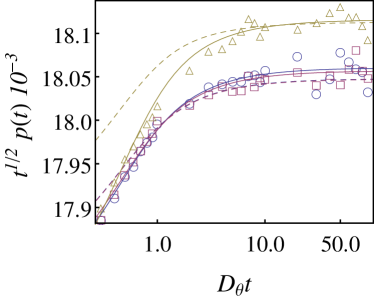
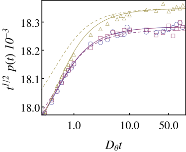
In order to validate the expression for the persistence probability we performed numerical simulations of Eq. 5. The initial condition was chosen from a Gaussian distribution with a very small width, so the sign of is clearly defined. The trajectories were evolved in time with an integration time-step of . At every instant, the survival of the particle trajectory was checked by looking at the sign of . Fraction of trajectories for which the position did not change its sign up to time gave the survival probability . A total of trajectories were used in estimating the survival probability. A comparison of the measured with that of the predictions of Eq. 27 is shown Fig. 2 and Fig. 3. Both the figures compare the persistence probability for weakly asymmetric particles. We observe that while the asymmetry of the particle is picked up as expected from our earlier work 32, for small propulsion velocity is unable to pick up the activity of the paricle. In the case when the activity of the particle is comparatively large, the indeed picks up the activity of the particle. When compared with the analytical expression of Eq. 27, for the small propulsion velocity, the expression compares quite well with the simulation resutls with the overall constant as the only fit parameter (the dotted lines in the figures). When the data is fitted to Eq. 27 with the overall constant fixed and and as fit parameters, it yeilds the correct values of and . However, for comparatively larger values of , when the expression is plotted against the numerical data with the overall constant as the only fit parameter, the data matches only asymptotically with the analytical expression. On the other hand, when the data is fitted with Eq. 27 with and as fit parameters, the fit yeilds a slightly lower value of and a slightly higher value of . For example, in the case of and (Fig. 2 open triangles), we obtain from the fit a value of and . In the case of and (Fig. 2 open triangles), we obtain from the fit a value of and .
Appendix C HARMONICALLY TRAPPED ASYMMETRIC PARTICLE
We now consider the case when such an active anisotropic particle is trapped in a harmonic trap. This situation typically occurs in the trapping and tracking of colloids in experiments. The harmonic potential is taken as isotropic potential with no preferred directional alignment.The potential is taken as . Using Eq. 5 the corresponding Langevin equation becomes
| (28) |
The correlations of the thermal fluctuations follow Eq. 6.
C.1 Perturbative expansion
Let us define the vector space , and the equation takes the general form as
| (29) |
In order to solve this equation we use the perturbative expansion
| (30) |
| (31) |
The formal solutions for Eq. 31 with the initial condition , becomes
| (32) |
The explicit form of the correlation matrix in the equal time, is given by
| (33) |
Here we have considered the fact that . We now start to calculate the different terms of the correlation matrix. The correlation matrix for averaged over the translational and the rotational noise is given as
| (34) |
The calculations of the time integrals in Eq. 34 have been explicitly shown in Appendix C (from Eq. C.1 to Eq. C.6) and the final result for is found as
| (35) |
In the limit of , Eq. 35 reproduces Eq. 11, the correct result for the free diffusion of active anisotropic particles.
We now proceed to calculate the correction term to this correlation and restrict ourselves only to the first order correction. To this end, we first restructure the solution of as
| (36) |
The correlation function is then given by
We now substitute the formal solution for as given in Eq. 32 and solve the integrals over time. The detailed calculation of LABEL:28a for the specific term is given in Appendix E. In evaluating the integrals, we have used the identity
| (38) |
Accordingly, the averages of the trigonometric functions over the rotational noise, which are used in the calculations, take the form
| (39) |
The final expression for is given by
| (40) |
Following Eq. 33, the mean-square displacement up to the first order correction is given by . From Eqs. 35 and 40 it is clear that the second term in Eq. 35 cancels with the first term in Eq. 40. Further, since we are interested in the expression for the mean square displacement up to the first order, the expression for becomes
| (41) |
Appendix D Persistence probability
We now want to calculate an expression for the persistence probability of an active anisotropic particle in the presence of a harmonic trap. As before, we first calculate the two-time correlation function of the -coordinate of the position vector. Keeping up to the first order correction in , the expression for the two time correlation function becomes , with . Note that the quantities and are only equal in the asymptotic limit, which is also the limit under consideration when evaluating the persistence probability. In Appendix D and Appendix E we have explicitly shown the calculations of the two terms that appear in the expression for the two-time correlation function . We merely quote the final expression here:
| (42) |
and
| (43) |
Choosing initial angle , all the terms in both the expressions for and survive. However, since we are interested in the asymptotic limit with , we drop the terms which are higher order exponentials in time and therefore decay faster. Further, since we are interested in the first order correction, we drop the second bracketed term in Eq. 43.
After a little algebra, the two-time correlation function for the -coordinate of the position vector, with initial angle becomes
| (44) |
where the effective trap constant is defined as As before, we define the variable and the correlation function of is given by
| (45) |
Using the time transformation for an imaginary time variable , such that
| (46) |
the two time correlation function in Eq. 45 transforms into a stationary correlator of the form and the persistence probability in the asymptotic limit in the imaginary variable is given by . Transforming back into real-time, the persistence probability becomes
| (47) |
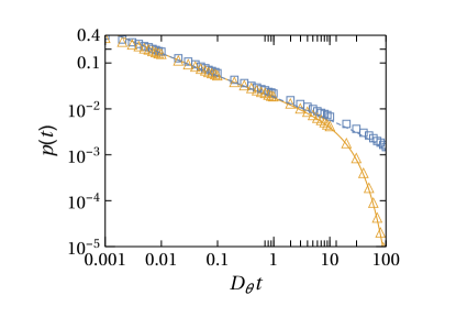
In the limit of , the equation correctly reproduces the result for a passive anisotropic particle. 32. In order to validate the equation, we performed numerical simulations of Eq. 28 with the initial condition chosen from a Gaussian distribution with a very small width, so that the sign of is well defined. The trajectories were evolved in time with an integration time step of . The persistence probability was determined from the fraction of trajectories for which did not change its sign. A comparison of the measured persistence probability is shown in Fig. 4 for two values . There is an excellent agreement of the measured survival probability with the analytical expression given in Eq. 47.
Appendix E Conclusion
In brief, we have calculated the persistence probability along the -axis of an active anisotropic particle in two dimensions in the absence of any potential and in the presence of a harmonic potential. The two-time correlation function has been calculated in the both cases. In the case of the harmonic trapped particle, we have used a perturbative solution for calculating the correlation functions. The persistence probability has been calculated with suitable space and time transformations. The anaytic expressions has been validated against numerically measured persistence probability.
References
- [1] Satya N Majumdar. Persistence in nonequilibrium systems. Current Science, 77(3):370–375, August 1999.
- [2] Satya N. Majumdar, Clément Sire, Alan J. Bray, and Stephen J. Cornell. Nontrivial exponent for simple diffusion. Phys. Rev. Lett., 77:2867–2870, Sep 1996.
- [3] T. J. Newman and Z. Toroczkai. Diffusive persistence and the “sign-time” distribution. Physical Review E, 58(3):R2685–R2688, September 1998.
- [4] Clément Sire, Satya N. Majumdar, and Andreas Rüdinger. Analytical results for random walk persistence. Phys. Rev. E, 61:1258–1269, Feb 2000.
- [5] D. Chakraborty and J. K. Bhattacharjee. Finite-size effect in persistence in random walks. Phys. Rev. E, 75:011111, Jan 2007.
- [6] D. Chakraborty. Persistence in random walk in composite media. The European Physical Journal B - Condensed Matter and Complex Systems, 64:263–269, 2008. 10.1140/epjb/e2008-00300-1.
- [7] D. Chakraborty. Time correlations and persistence probability of a Brownian particle in a shear flow. The European Physical Journal B, 85(8):281, aug 2012.
- [8] D. Chakraborty. Persistence of a Brownian particle in a time-dependent potential. Physical Review E, 85(5):051101, may 2012.
- [9] D. Chakraborty. Persistence in advection of a passive scalar. Phys. Rev. E, 79:031112, Mar 2009.
- [10] Francesco Mori, Pierre Le Doussal, Satya N. Majumdar, and Grégory Schehr. Universal survival probability for a -dimensional run-and-tumble particle. Phys. Rev. Lett., 124:090603, Mar 2020.
- [11] Bernard Derrida, Vincent Hakim, and Vincent Pasquier. Exact first-passage exponents of 1d domain growth: Relation to a reaction-diffusion model. Phys. Rev. Lett., 75:751–754, Jul 1995.
- [12] Robert Stephen Cantrell, Chris Cosner, and Salomé Martínez. Persistence for a two-stage reaction-diffusion system. Mathematics, 8(3), 2020.
- [13] GI Menon, S Sinha, and P Ray. Persistence at the onset of spatio-temporal intermittency in coupled map lattices. EPL (Europhysics Letters), 27:1–8, 2003.
- [14] Satya N. Majumdar and Clément Sire. Survival probability of a gaussian non-markovian process: Application to the dynamics of the ising model. Phys. Rev. Lett., 77:1420–1423, Aug 1996.
- [15] Satya N. Majumdar and Alan J. Bray. Persistence with partial survival. Phys. Rev. Lett., 81:2626–2629, Sep 1998.
- [16] Malte Henkel and Michel Pleimling. Non-markovian global persistence in phase ordering kinetics. Journal of Statistical Mechanics: Theory and Experiment, 2009(12):P12012, dec 2009.
- [17] J. Krug, H. Kallabis, S. N. Majumdar, S. J. Cornell, Alan J. Bray, and C. Sire. Persistence exponents for fluctuating interfaces. Phys. Rev. E, 56:2702–2712, Sep 1997.
- [18] H. Kallabis and J. Krug. Persistence of kardar-parisi-zhang interfaces. EPL (Europhysics Letters), 45(1):20, 1999.
- [19] Z. Toroczkai, T. J. Newman, and S. Das Sarma. Sign-time distributions for interface growth. Phys. Rev. E, 60:R1115–R1118, Aug 1999.
- [20] Satya N. Majumdar and Alan J. Bray. Spatial persistence of fluctuating interfaces. Phys. Rev. Lett., 86:3700–3703, Apr 2001.
- [21] Satya N. Majumdar, Alan J. Bray, S. J. Cornell, and C. Sire. Global persistence exponent for nonequilibrium critical dynamics. Phys. Rev. Lett., 77:3704–3707, Oct 1996.
- [22] D. Chakraborty and J. K. Bhattacharjee. Global persistence exponent in critical dynamics: Finite-size-induced crossover. Physical Review E, 76(3):031117, sep 2007.
- [23] D. S. Dean and Satya N Majumdar. Extreme-value statistics of hierarchically correlated variables deviation from Gumbel statistics and anomalous persistence. Physical Review E, 64(4):046121, sep 2001.
- [24] Somnath Bhattacharya, Dibyendu Das, and Satya N. Majumdar. Persistence of a rouse polymer chain under transverse shear flow. Phys. Rev. E, 75:061122, Jun 2007.
- [25] F. Ren, B. Zheng, H. Lin, L.Y. Wen, and S. Trimper. Persistence probabilities of the german dax and shanghai index. Physica A: Statistical Mechanics and its Applications, 350(2):439–450, 2005.
- [26] M. Constantin and S. Das Sarma. Volatility, persistence, and survival in financial markets. Phys. Rev. E, 72:051106, Nov 2005.
- [27] B. Yurke, A. N. Pargellis, Satya N. Majumdar, and C. Sire. Experimental measurement of the persistence exponent of the planar ising model. Phys. Rev. E, 56:R40–R42, Jul 1997.
- [28] Glenn P. Wong, Ross W. Mair, and Ronald L. Walsworth. Measurement of Persistence in 1D Diffusion. Physical Review Letters, 86(18):4156–4159, apr 2001.
- [29] Yael Efraim and Haim Taitelbaum. Persistence in reactive-wetting interfaces. Physical Review E, 84(5):370–4, November 2011.
- [30] Alan J. Bray, Satya N. Majumdar, and Grégory Schehr. Persistence and first-passage properties in nonequilibrium systems. Advances in Physics, 62(3):225–361, 2013.
- [31] D. Slepian. The one-sided barrier problem for gaussian noise. Bell System Tech. J, 41(2):463–501, 1962.
- [32] Anirban Ghosh and Dipanjan Chakraborty. Persistence in brownian motion of an ellipsoidal particle in two dimensions. The Journal of Chemical Physics, 152(17):174901, 2020.
- [33] Amir Shee and Debasish Chaudhuri. Self-propulsion with speed and orientation fluctuation: Exact computation of moments and dynamical bistabilities in displacement. Phys. Rev. E, 105:054148, May 2022.
Appendix A Mean-square displacement of a active anisotropic free particle
| (A.1) |
Integral is having two separate integrals and solving these two separately
| (A.2) |
and
| (A.3) |
| (A.4) |
Now the second integral of Eq. (Eq. 10) is calculated as
| (A.5) |
Using the explicit form of from Eq. (Eq. 7) the mean-square displacement along the - direction becomes
| (A.6) |
Appendix B Calculation of two-time Correlation for a free active anisotropic particle
| (B.1) |
for
for
Lets take the two integrals of Eq.(Eq. B.1) as and . The integral Eq.(Eq. B.1) can be calculated in general terms like,
for integral ,
and for integral ,
So final form of becomes
| (B.2) |
The second integral of Eq. 10 is solved as
| (B.3) |
Appendix C Calculation of for a harmonically trapped particle
| (C.1) |
There are two integrals, lets say and respectively. Lets calculate these two separately
| (C.2) |
For -direction
| (C.3) |
| (C.4) |
Lets solve the integrals separately
| (C.5) |
| (C.6) |
Appendix D Calculation of
| (D.1) |
The case of corresponds to and the explicit form of the correlation becomes
| (D.2) |
It can be calculated as two separately and integrals
| (D.3) |
| (D.4) |
Lets calculate integrals separately
| (D.5) |
| (D.6) |
| (D.7) |
Appendix E Calculation of
We now turn our attention to the first order correction that enter the correlation matrix. Using the formal solution for we write down
| (E.1) |
We evaluate the two terms in the integral separately. The first term involves an average over the thermal fluctuations in the position and we denote it by . The explicit calculation of becomes
| (E.2) |
In order to proceed further with the calculation, We consider the correlation function so that the above expression becomes
| (E.3) |
The second term of Eq. E.1 is denoted by and is given as
| (E.4) |
so that for the correlation function Eq. E.4 transforms as
| (E.5) |
We use the following trignometric identities
| (E.6) |
to rewrite the triple product of the trignometric functions, averaged over the rotational noise as
| (E.7) |
Note that in the above set of equations, the time dependence in the right hand side of the set of equations (a)–(d) is identical to the set of equations (e)–(h). Let us calculate Eq.(Eq. E.2) by using Eq.(Eq. E.7), at first we take the first term (a), and calculate separately
| (E.8) |
Here in the above integral always and in the first case let us take we get
Case(1),
| (E.9) |
Case(2),
| (E.10) |
Adding Eq.(Eq. E.9) and Eq.(Eq. E.10) terms we get the term Eq.(Eq. E.8) as,
| (E.11) |
The way first term has been calculated similiarly other terms are calculated to find the exact expression of Eq.(Eq. E.5). The results of Integrals due to terms (b), (c), and (d) are as follows
| (E.12) |
| (E.13) |
| (E.14) |
Integral values to due term (e) will be same of (a) similarly others. Terms due to (f), (g), (h) of Eq.(Eq. E.7) will be zero for the initial orientational angle . Now for the simplification we are taking only the term associated with of Eq.(Eq. E.11). Similarly another same term of will arise due to the contribution of (e) of Eq.(Eq. E.7).
After adding the relevant terms, the final expression for the two-time correlation term becomes,
| (E.15) |
From the above equation, the first order correction in is given by
| (E.16) |