Millimeter Gap Contrast as a Probe for Turbulence Level in Protoplanetary Disks

Abstract

Turbulent motions are believed to regulate angular momentum transport and influence dust evolution in protoplanetary disks. Measuring the strength of turbulence is challenging through gas line observations because of the requirement for high spatial and spectral resolution data, and an exquisite determination of the temperature. In this work, taking the well-known HD 163296 disk as an example, we investigated the contrast of gaps identified in high angular resolution continuum images as a probe for the level of turbulence. With self-consistent radiative transfer models, we simultaneously analyzed the radial brightness profiles along the disk major and minor axes, and the azimuthal brightness profiles of the B67 and B100 rings. By fitting all the gap contrasts measured from these profiles, we constrained the gas-to-dust scale height ratio $\Lambda$ to be $3.0_{-0.8}^{+0.3}$, $1.2_{-0.1}^{+0.1}$ and ${\geq}\,6.5$ for the D48, B67 and B100 regions, respectively. The varying gas-to-dust scale height ratios indicate that the degree of dust settling changes with radius. The inferred values for $\Lambda$ translate into a turbulence level of $\alpha_{\rm turb}\,{<}\,3\times 10^{-3}$ in the D48 and B100 regions, which is consistent with previous upper limits set by gas line observations. However, turbulent motions in the B67 ring are strong with $\alpha_{\rm turb}\,{\sim}1.2\,{\times}\,10^{-2}$. Due to the degeneracy between $\Lambda$ and the depth of dust surface density drops, the turbulence strength in the D86 gap region is not constrained.

97.82.Jw, 95.30.Jx, 97.82.Fs

1 Introduction

Protoplanetary disks, as the birthplace of planetary systems, always exhibit turbulent motions [1]. There are several mechanisms currently discussed as main contributors: hydrodynamical instabilities as the vertical shear instability [2, 3, 4], convective overstability [5, 6], Zombie vortex stability [7, 8], and magneto-hydrodynamical instabilities like the magnetorotational instability [9, 10, 11]. Turbulence regulates the angular momentum transport to sustain gas accretion onto the central star [12, 13], influences the evolution of dust grains in disks [14], and plays an important role in controlling the dynamics of embedded planets [15]. Hence, a detailed understanding of disk evolution and planet formation requires knowledge of the strength of turbulent motions.

Placing constraints on the turbulence level is also important in interpreting observational data with numerical simulations. In recent years, high-resolution images at infrared and (sub-)millimeter wavelengths have shown that gaps and rings are frequently observed in planet-forming disks [16, 17, 18]. These interesting substructures are often thought to be created by planet-disk interaction [19, 20, 21]. The description of the underlying physics relies heavily on (magneto-)hydrodynamical simulations in which turbulence strongly affects the resulting depth and number of gaps [22, 23, 24, 25, 26]. As a consequence, the inferred properties (e.g., mass and location) and number of the “unseen” (proto)planets are dependent on the input strength of turbulence in the simulation.

However, measuring turbulence with gas line observations is very challenging because on the one hand it demands for data at high spatial and spectral resolution, and on the other hand thermal motion usually dominates the broadening of lines, leading to substantial difficulties when separating its contribution from the measured total line width [27]. Therefore, the measurement of turbulence via gas line data so far is limited to a small number of disks, revealing low turbulent velocities typically below $5\%\,{\sim}\,10\%$ of the local sound speed ($c_{s}$) [28, 29, 30, 31, 32]. An exception is for the DM Tau disk, where the measured turbulent velocity approaches $0.25\,{\sim}\,0.33\,c_{s}$ [32].

Turbulence also affects the motion of the dust, either in the radial direction or in the vertical one. Dullemond & Penzlin [33] suggested that the dependence of turbulence on the dust-to-gas mass ratio together with the radial drift of dust particles could be the origin of the ring structures commonly found in protoplanetary disks. By comparing the width of the millimeter continuum emission ring with the pressure scale height of the disk, Dullemond et al. [34] found strong evidence of dust trapping operating in all the rings analyzed in their sample, and put constraints on the quantity $\alpha_{\rm turb}/{\rm St}$, where $\alpha_{\rm turb}$ is the turbulence parameter, and $\rm{St}$ is the Stokes number of the dust particles. Vertical stirring induced by turbulent motions acts as a counter process against the settling of dust grains. Theoretically speaking, millimeter continuum emission is dominated by millimeter-sized dust particles that are located near the midplane of the disk. However, material residing in the adjacent rings, located above the midplane, would hide the gap due to beam smearing. How severe this smoothening effect is depends on the scale height of millimeter-sized dust grains [35]. In stronger turbulent disks, dust grains are more vertically distributed, leading to a more substantial reduction on the gap depth.

Recently, Doi & Kataoka [36] discussed the feasibility of analyzing the intensity variation as a function of azimuth on the rings to estimate the degree of dust settling. When the disk is optically thin and viewed at an oblique inclination, the optical depth $\tau$ along the line of sight on the major and minor axes differs from each other. Such a difference in $\tau$ forms a peak and dip in the brightness profile at the azimuthal angle of the major and minor axis, respectively. The ratio between the brightness peak and dip depends on the millimeter dust scale height. The authors fit the azimuthal brightness profiles of two rings in the HD 163296 disk, and constrained the gas-to-dust scale height ratio and therefore the turbulence level. In their analysis, the disk is assumed to be vertically isothermal with a fixed midplane temperature profile. How such a simplification affects the result, particularly for rings with a large millimeter dust scale height (i.e., high turbulence regions) needs to be investigated.

In this work, we take the HD 163296 disk as an example to investigate in detail the link between millimeter gap contrasts and the strength of turbulence, and highlight some features and degeneracies that can be encountered. Sect. 2 gives an introduction about the HD 163296 disk. The modeling assumptions are presented in Sect. 3, while the process of dedicated fitting to the ALMA image is described in Sect. 4. We discuss our results in Sect. 5. The paper ends up with a summary in Sect. 6.

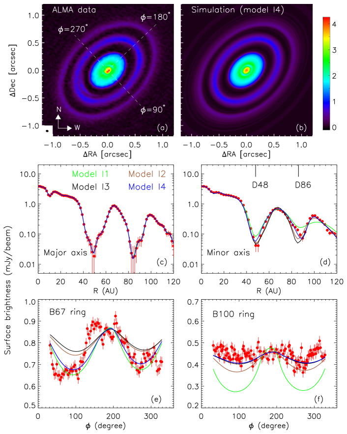
Figure 1: A comparison between models and the DSHARP observation of the HD 163296 disk. Panel (a): fiducial image generated by the DSHARP team. The beam is shown as the black ellipse in the bottom left corner. The dashed lines indicate the semi-major (to the northwest) and minor axes of the disk. The values of the azimuth ($\phi$) for the disk major and minor axes are given for a reference of the coordinate. Panel (b): the simulated image of the best-fit model (i.e., model I4). Panel (c)-(f): a comparison of brightness profiles between observation and different models. The red dots refer to data points, whereas the green, brown, black and blue lines represent model I1, I2, I3 and I4, respectively. Model parameters can be found in Table 2, and model gap contrasts are compared with the observation in Table 1. Note that the four models overlap well with each other in panel (c).

2 Circumstellar disk of HD 163296

HD 163296 is a Herbig Ae star (A1 spectral type) located at a distance of $D\,{=}\,101\,{\pm}\,2\,\rm{pc}$ [37]. Its mass ($M_{\star}$) and age are $1.9\,M_{\odot}$ and $10.4\,\rm{Myr}$ [38]. It has a luminosity of $L_{\star}\,{=}\,17\,L_{\odot}$, and an effective temperature of $T_{\rm eff}\,{=}\,9250\,\rm{K}$ [39]. Spatially resolved observations at both infrared and millimeter regimes have revealed ring structures in the disk around HD 163296 [40, 41, 42, 43, 44]. Analysis of the interferometric data taken with the Very Large Telescope Interferometer PIONIER and MATISSE yielded brightness asymmetries in the near-infrared emission, which may originate from a vortex near the inner rim ($R\,{\sim}\,0.4\,\rm{AU}$) of the disk [45, 46].

As one of the 20 targets selected in the Disk Substructures at High Angular Resolution Program (DSHARP), HD 163296 was observed with the Atacama Large Millimeter/submillimeter Array (ALMA) in Band 6 at an unprecedented spatial resolution of $4.8\,{\times}\,3.8\,\rm{AU}$ [18]. The rms noise of the fiducial ALMA image generated by the DSHARP team is $\sigma_{\rm rms}\,{=}\,23\,\mu{\rm Jy/beam}$. The continuum image shows a few pairs of concentric rings/gaps, see panel (a) in Figure 1. The D48 and D86 gaps are located at a radial distance of 48 and 86 AU, with a width of 20 and 16 AU, respectively. The B67 and B100 rings are centered at a radial distance of 67 and 100 AU, with a width of 16 and 12 AU, respectively [47].

We extracted the surface brightness along the disk major and minor axes, given the position angle (PA) of $133.33^{\circ}$. Along a PA of $99^{\circ}$, there is a crescent-like structure centered at a radial distance of $55\,\rm{AU}$ [48], which is probably caused by a Jupiter mass planet [49]. Such an asymmetry contaminates the measurement of the gap contrast. Hence, we only considered the data on the semi-major axis to the northwest. On the minor axis, however, an average of both sides of the disk was performed to improve the signal-to-noise ratio. To apply the methodology introduced by Doi & Kataoka [36], we also extracted the azimuthal brightness profiles on the B67 and B100 rings. The reference for the azimuthal coordinate ($\phi$) is given in panel (a) of Figure 1. The extracted brightnesses are shown with red dots in panels (c)-(f) of Figure 1. It should be noted that the mechanism responsible for generating the crescent-like structure also likely causes azimuthal perturbations to the B67 ring, which may be one of the reasons why the brightness profile shows non-axisymmetric features. The width between two adjacent points (i.e., 1.5 AU) is about one third of the ALMA beam, which means that the brightness is first averaged over such a bin size and then extracted. The errors for each of the data points on the major axis, B67 and B100 rings are all set to $23\,\mu{\rm Jy/beam}$, but on the minor axis they are calculated to be $\frac{23}{\sqrt{2}}\,\mu{\rm Jy/beam}$ due to the average of both sides of the disk.

Table 1: Gap contrasts of the HD 163296 disk.

	Major axis		Minor axis		B67 ring		B100 ring
4
6
8
	D48	D86	D48	D86	$\phi=90^{\circ}$	$\phi=270^{\circ}$	$\phi=90^{\circ}$	$\phi=270^{\circ}$
ALMA data	$0.98\,{\pm}\,0.03$	$0.96\,{\pm}\,0.05$	$0.94\,{\pm}\,0.02$	$0.82\,{\pm}\,0.04$	$0.22\,{\pm}\,0.03$	$0.21\,{\pm}\,0.03$	$0.00\,{\pm}\,0.07$	$0.15\,{\pm}\,0.07$
Model I1	0.97	0.97	0.88	0.34	0.24	0.21	0.42	0.41
Model I2	0.97	0.97	0.94	0.80	0.13	0.11	0.20	0.18
Model I3	0.97	0.97	0.94	0.87	0.11	0.10	0.11	0.11
Model I4	0.97	0.97	0.92	0.81	0.21	0.18	0.10	0.10

The gap contrast is defined as $1\,{-}\,I_{\rm min}/I_{\rm max}$, where $I_{\rm min}$ is the minimum brightness within the gap, and $I_{\rm max}$ is the maximum brightness of its immediately exterior ring. The brightness profile of the B67 ring displays two dips at $\phi\,{=}\,90^{\circ}$ and $270^{\circ}$, which resemble gaps. For simplicity of description, we also call them as “gaps” hereafter in this work. The constrasts are defined as $1\,{-}\,I_{\phi{=}90^{\circ}}/I_{\phi{=}180^{\circ}}$ and $1\,{-}\,I_{\phi{=}270^{\circ}}/I_{\phi{=}180^{\circ}}$. On the B100 ring, the profile is quite flat in the western side, and shows only one “gap” at $\phi\,{=}\,270^{\circ}$. In addition to the chi-square ($\chi^{2}$) metrics, the observed gap contrasts summarized in Table 1 are the key characteristics used to evaluate the quality of fit of our models. The difference between gap contrasts measured along the disk major and minor axes is due to projection effect. Because the disk is geometrically thick, and it is tilted to an inclination of $46.7^{\circ}$, the width of the gap varies with azimuthal angle, and reaches the smallest along the minor axis, leading to the lowest gap contrast.

3 Full radiative transfer modeling

The key of our work is to constrain the scale height of the millimeter-sized dust grains by fitting the contrasts of gaps with self-consistent radiative transfer models, and then link the scale height to the strength of turbulence. In fact, the HD 163296 disk has more gaps, i.e., D10 and D145. However, they are either not fully spatially resolved, or show evidence for being multiple gaps [47]. We will not discuss them in detail throughout the paper, although our modeling methodology automatically captures both features.

The radiative transfer models are parameterized in the framework of the RADMC-3D code [50]. We assume that the disk is passively heated by stellar irradiation. The stellar spectrum is taken from the Kurucz database [51], assuming a gravity of ${\rm log}\,g\,{=}\,3.5$ and solar metallicity. Other model assumptions are for the density distribution and dust opacities, which are described below.

3.1 Dust density distribution

We consider a disk that extends from an inner to outer radii of $R_{\rm in}\,{=}\,0.4\,\rm{AU}$ and $R_{\rm out}\,{=}\,169\,\rm{AU}$, respectively [47]. The model has two distinct dust grain populations, i.e., a small grain population (SGP) and a large grain population (LGP). The temperature structure of the disk is mainly governed by the SGP, whereas the LGP dominates the millimeter continuum emission. We fixed the mass fraction of the LGP to $f_{\rm SGP}\,{=}\,0.85$ that has been commonly used in previous modeling works of protoplanetary disks [52, 53]. The SGP is assumed to be well-mixed with the underlying gas distribution. Therefore, its scale height is set to the gas scale height ($H_{\rm gas}$) that is solved under the condition of vertical hydrostatic equilibrium. Large dust grains are expected to settle towards the midplane [54, 55]. We characterize the degree of dust settling with the parameter $\Lambda$, and the scale height of the LGP is given by $H_{\rm gas}/{\Lambda}$.

The volume density of the dust grains is parameterized as

$$\rho_{\rm{SGP}}(R,z)\,{=}\,\frac{(1-f_{\rm LGP})\,\Sigma_{\rm d}(R)}{\sqrt{2\pi}\,H_{\rm gas}}\,\exp\left[-\frac{1}{2}\left(\frac{z}{H_{\rm gas}}\right)^{2}\right],\\$$ (1)

$$\rho_{\rm{LGP}}(R,z)\,{=}\,\frac{f_{\rm LGP}\,\Sigma_{\rm d}(R)}{\sqrt{2\pi}\,H_{\rm gas}/{\Lambda}}\,\exp\left[-\frac{1}{2}\left(\frac{z}{H_{\rm gas}/{\Lambda}}\right)^{2}\right],\\$$ (2)

where $\Sigma_{\rm d}(R)$ is the dust surface density, and $R$ is the distance from the central star measured in the disk midplane. Literatural studies usually took analytic forms for $\Sigma_{d}(R)$, e.g., a power law or power law with an exponential taper. However, such simple expressions have been demonstrated to be insufficient to capture the fine-scaled features revealed by high resolution ALMA observations [35, 56]. Instead, we build the surface density by iteratively fitting the surface brightnesses at the ALMA wavelength where the optical depth is generally low, see Sect. 3.3.

3.2 Dust properties

For the dust composition, we made use of the recipe by the DiscAnalysis (DIANA) project [57]. The dust grains consist of 60% silicate ($\rm{Mg_{0.7}Fe_{0.3}SiO_{3}}$) [58], 15% amorphous carbon (BE$-$sample) [59], and 25% porosity. These percentages are volume fractions of each component, which are used to derive the effective refractory indices of the dust ensemble by applying the Bruggeman mixing rule [60]. We used a distribution of hollow spheres with a maximum hollow volume ratio of 0.8 [61]. The mean solid density of the dust ensemble $\rho_{\rm grain}\,{=}\,2.1\,\rm{g\,cm}^{-3}$ is estimated from an average between the silicate density ($3.01\,\rm{g\,cm}^{-3}$) and carbon density ($1.8\,\rm{g\,cm}^{-3}$) taking the volume fractions as the weighting factors.

The distribution of grain sizes ($a$) follows a power law ${\rm d}n(a)\,{\propto}\,{a^{-3.5}}{\rm d}a$ with a minimum ($a_{\rm{min}}$) and maximum size ($a_{\rm{max}}$). For the SGP, $a_{\rm{min}}$ and $a_{\rm{max}}$ are fixed to $0.01\,\mu{\rm m}$ and $2\,\mu{\rm m}$, respectively. For the LGP, $a_{\rm{min}}$ is set to $2\,\mu{\rm m}$. Regarding $a_{\rm{max}}$, we will set it based on models that can reproduce the observed millimeter spectral slope, see Sect. 3.4.

3.3 Building the dust surface density

Previous studies have shown that surface density profiles in simple analytic expressions (e.g., a smooth power law with density drops at the gap locations) have difficulties to capture the detailed features revealed by ALMA [56, 42]. Using an iterative procedure, we built the surface densities by reproducing the millimeter surface brightnesses along the disk major axis that features the maximum spatial resolution. This approach was introduced by Pinte et al. [35], and several works by other teams demonstrated its success [42, 21]. The iterative process consists of the following steps.

• We took a starting surface density profile $\Sigma_{\rm d}(R)\,{=}\,\Sigma_{0}\left(R/R_{\rm c}\right)^{-\gamma}{\rm exp}\left[-(R/R_{\rm c})^{2-\gamma}\right]$ with $R_{\rm{c}}\,{=}\,90\,\rm{AU}$ and $\gamma\,{=}\,0.1$ [43]. For the starting point, we did not introduce any gap, and using other forms will not have a significant impact to the final result.

• With an initial guess for $H_{\rm gas}$, the dust density distribution is given by Eq. 1 and 2. Radiative transfer modeling is performed to obtain the dust temperature. Then, the dust density structure is solved assuming that the disk is in vertical hydrostatic equilibrium. We run the radiative transfer modeling with the new dust density distribution to get the new dust temperature. The iteration for the dust temperature and density goes back and forth, and convergence can be achieved after ${\sim}\,5$ iterations. For the initial choice of $H_{\rm gas}$, we assume $H_{\rm gas}\,{=}\,\sqrt{kT(R)R^{3}/GM_{\star}{\mu}m_{p}}$, where $G$ is the gravitational constant, $k$ is the Bolzmann’s constant, $m_{p}$ is the mass of proton, $\mu\,{=}\,2.3$ is the mean molecular weight, and $T(R)=18.7(R/400\,\rm{AU})^{-0.14}$ is the midplane temperature given by Dullemond et al. [62]. The black solid line in Figure 6 shows the initial $H_{\rm gas}$. This step is time consuming because a smooth temperature structure is required to get the solution for the corresponding dust density. Thus, we use a total number of $3\,{\times}\,10^{7}$ photons in the simulation.

• From step b), the gas scale height ($H_{\rm gas}$) is derived self-consistently. Then, we simulate a model image at 1.25 mm, which is convolved with the ALMA beam that has a size and position angle of $0.048^{\prime\prime}\times 0.038^{\prime\prime}$ and $82^{\circ}$, respectively.

• We extracted the model surface brightness along the disk major axis to the northwest, identical to what we have done on the ALMA image.

• A ratio as a function of radius $\zeta(R)$ is obtained by dividing the observed brightness profile by the model brightness profile.

• The surface densities used as the input for the model is scaled by the point-by-point ratios $\zeta(R)$. The process goes back to step b.

The iteration for $\Sigma_{\rm d}$ typically converges after about 25 loops, when the change in the model brightness profile is less than 5% at all radii.

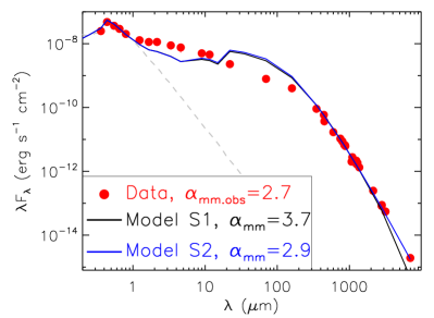
Figure 2: SED of the HD 163296 disk. Red dots indicate photometric data that are taken from literature. The black and blue lines show two models with the maximum grain size being $a_{\rm max}\,{=}\,1\,\rm{mm}$ and 1 cm, respectively. The grey dashed line denotes the photospheric spectrum. The spectral indices measured at wavelengths $\lambda\,{\geq}\,1\,\rm{mm}$ are given for both the models and observation.

Table 2: Overview of parameter values for different models.

Parameter	Fixed/free	Model S1	Model S2	Model I1	Model I2	Model I3	Model I4	Note
$T_{\rm eff}$ [K]	Fixed	9250						Effective temperature
$L_{\star}\,[L_{\odot}]$	Fixed	17						Stellar luminosity
$D$ [pc]	Fixed	101						Distance
$i\,[^{\circ}]$	Fixed	46.7						Disk inclination
${\rm PA\,[^{\circ}]}$	Fixed	133.33						Position angle
$R_{\rm in}$ [AU]	Fixed	0.4						Disk inner radius
$R_{\rm out}$ [AU]	Fixed	169						Disk outer radius
$f_{\rm LGP}$	Fixed	0.85						Mass fraction of the LGP
$a_{\rm min.SGP}$ [$\mu{\rm m}$]	Fixed	0.01						Minimum grain size for the SGP
$a_{\rm max.SGP}$ [$\mu{\rm m}$]	Fixed	2						Maximum grain size for the SGP
$a_{\rm min.LGP}$ [$\mu{\rm m}$]	Fixed	2						Minimum grain size for the LGP
$a_{\rm max.LGP}$ [cm]	Free	0.1	1.0	1.0	1.0	1.0	1.0	Maximum grain size for the LGP
$\Sigma_{\rm d}\,\rm{[g\,cm^{-2}]}$	Free	Figure 7	Figure 7	Figure 3	Figure 3	Figure 3	Figure 3	Dust surface density
$M_{\rm dust}\,[10^{-4}\,M_{\odot}]$ (a)	$-$	1.2	2.4	2.3	2.4	2.4	2.5	Total dust mass
$\Lambda$	Free	5.0	5.0	1.0	2.6	10.6	$-$	$\Lambda$ for the entire disk, see Sect. 4.1
$\Lambda{1}$	Free	$-$	$-$	$-$	$-$	$-$	$3.0_{-0.8}^{+0.3}$	$\Lambda$ for ${R\,{<}\,59\,\rm{AU}}$, see Sect. 4.2
$\Lambda{2}$	Free	$-$	$-$	$-$	$-$	$-$	$1.2_{-0.1}^{+0.1}$	$\Lambda$ for ${59\,{\leq}\,R\,{<}\,78\,\rm{AU}}$, see Sect. 4.2
$\Lambda{3}$	Free	$-$	$-$	$-$	$-$	$-$	$1.9_{-0.1}^{+15.9}$	$\Lambda$ for ${78\,{\leq}\,R\,{<}\,94\,\rm{AU}}$, see Sect. 4.2
$\Lambda{4}$	Free	$-$	$-$	$-$	$-$	$-$	$16.3_{-9.8}^{+3.7}$	$\Lambda$ for ${R\,{\geq}\,94\,\rm{AU}}$, see Sect. 4.2
$\chi_{\rm tot}^{2}$	$-$	$-$	$-$	975	460	478	242	Chi-square of the model, see Eq. 3

• The total dust mass $M_{\rm dust}$ is obtained by integrating the surface density $\Sigma_{\rm d}$ that is constructed in the fitting procedure. Hence, $M_{\rm dust}$ is not a direct fitting parameter.

3.4 Setting $a_{\rm{max}}$ for the LGP based on SED modeling

Our model has three free parameters/quantities: the dust surface density ($\Sigma_{\rm d}$), the ratio of gas-to-dust scale height ($\Lambda$) and maximum grain size ($a_{\rm max}$) for the LGP. Note that the total dust mass ($M_{\rm dust}$) is not a free parameter, because integrating $\Sigma_{\rm d}$ within the disk naturally gives the result.

A population of large dust grains will shallow the spectral index at millimeter wavelengths [63, 64]. We collected photometric data from various catalogs and individual studies [65, 66, 67, 68, 69, 70, 71, 72, 73, 18, 74]. The observed spectral energy distribution (SED) is shown as red dots in Figure 2. The spectral index measured at wavelengths $\lambda\,{\geq}\,1\,\rm{mm}$ is $\alpha_{\rm mm.obs}\,{=}\,2.7\,{\pm}\,0.06$. Assuming that the emission is optically thin and in the Rayleigh-Jeans tail, this transfers into a millimeter slope of the dust absorption coefficient $\beta\,{=}\,\alpha_{\rm mm.obs}{-}\,2\,{=}\,0.7$. The $\beta$ value for the interstellar medium dust is ${\sim}\,1.7$ [75]. A lower $\beta$ in the HD 163296 disk suggests that dust grains have grown up to millimeter and even centimeter sizes.

To quantify the extent of grain growth in the HD 163296 disk, we build a grid of SED models in which the ratio of gas-to-dust scale height is fixed to $\Lambda\,{=}\,5$, a typical value used in literature works [52, 53]. In Sect. 4, we will conduct an extensive parameter study on $\Lambda$ through a dedicated fitting to the ALMA image. However, this parameter is not expected to have a significant impact to the constraint on $a_{\rm max}$ as long as the optical depth is not large. We sample 16 different $a_{\rm max}(s)$ that are logarithmically distributed from $10\,\mu{\rm m}$ to 1 cm. The procedure of iteration for $\Sigma_{\rm d}$, as laid out in Sect. 3.3, is performed separately for each of the 16 models. As a result, 16 model SEDs are simulated. The model with $a_{\rm max}\,{=}\,1\,\rm{cm}$ (Model S2) best matches with the observation, see Figure 2. Its converged surface density is shown in Figure 7, and Table 2 gives an overview of the model parameters. For the subsequent fitting to the ALMA data, we fixed $a_{\rm max}\,{=}\,1\,\rm{cm}$ for the LGP, leaving $\Sigma_{\rm d}$ and $\Lambda$ as the only two free parameters.

The discrepancies in the mid- and far-infrared fluxes between model and observation is due to the presence of a puffed-up inner rim. This type of rim is a natural outcome when solving the disk structure in vertical hydrostatic equilibrium, particularly for Herbig disks [76]. The blue solid line in Figure 6 shows the gas scale height of Model S2. The overall geometry of the disk is flared. Disk regions just behind the inner rim cannot be exposed to the stellar light, leading to a reduced mid-infrared excess. At a certain radial distance, the disk will show up from the shadow casted by the inner rim. The surface layer of these outer regions directly absorbs stellar photons, and hence produces more far-infrared emission than the observed level. One can fully parameterize the scale height with analytic forms, e.g., a power law, and fit the infrared SED to constrain the geometry [77]. However, there are some degeneracies between the geometric parameters in SED models. Moreover, modeling the SED is not able to constrain the scale height of millimeter dust grains that is the key of this work. Therefore, we do not attempt to conduct further fine tuning on the SED fitting, and make our assumptions (i.e., number of free parameters) as few as possible.

4 Fitting the DSHARP ALMA image

In this section, we will fit the surface brightnesses along the major and minor axes of the disk, and on the B67 and B100 rings to constrain $\Lambda$. Our strategy starts from a simple assumption of a constant $\Lambda$ in the radial direction, to a more complex scenario in which $\Lambda$ varies with $R$.

The contrasts of gaps, as presented in Table 1, are sensitive to the degree of dust settling. Therefore, to quantify the quality of fit, we first check whether or not the gap contrasts of the model are consistent with the observation. Then, we calculate the $\chi^{2}$ along the major axis ($\chi_{\rm major}^{2}$) and minor axis ($\chi_{\rm minor}^{2}$), and on the B67 ($\chi_{\rm B67}^{2}$) and B100 ring ($\chi_{\rm B100}^{2}$). To exclude the effect of the crescent-like substructure along ${\rm PA}\,{\sim}\,99^{\circ}$, data points between $\phi\,{=}\,{-}45^{\circ}$ and $45^{\circ}$ are not taken into account when calculating $\chi_{\rm B67}^{2}$ and $\chi_{\rm B100}^{2}$. The goodness of fit is evaluated according to

$$\chi_{\rm tot}^{2}\,{=}\,g_{1}\,\chi_{\rm major}^{2}+g_{2}\,\chi_{\rm minor}^{2}+g_{3}\,\chi_{\rm B67}^{2}+g_{4}\,\chi_{\rm B100}^{2}.$$ (3)

Four factors, i.e., $g_{1}$, $g_{2}$, $g_{3}$ and $g_{4}$, are introduced to balance the weightings. First, we calculate the factors as

$$g_{i}=\frac{\sum_{i=1}^{4}\left(N_{i}\right)}{N_{i}},$$ (4)

where $N_{i}$ is the number of data points taken into account in the calculation of $\chi^{2}(s)$ for the major and minor axes, and the B67 and B100 rings, respectively. Then, a normalization is performed to ensure that the sum of $g_{i}$ equals to unity.

4.1 Constant $\Lambda$ in the radial direction

We first take the simplest assumption in which the ratio of gas-to-dust scale height does not change with radius ($R$). We sample 20 values for $\Lambda$, which are logarithmically distributed within 1 and 20. The case of $\Lambda\,{=}\,1$ means that millimeter dust grains are well coupled with the gas. Strongly settled models feature large values of $\Lambda$. The iteration process for $\Sigma_{d}$ is performed from scratch for each of these 20 models, ensuring that all the models are fully independent and self-consistent.

None of the 20 models can reproduce all of the gap constrasts within the uncertainties simultaneously. Panels (c)-(f) of Figure 1 shows a comparison of the brightnesses between observation and three representative models with $\Lambda\,{=}\,1.0$ (model I1), 2.6 (model I2) and 10.6 (model I3), respectively. Model I2 has the lowest $\chi_{\rm tot}^{2}\,{=}\,460$ among the 20 samples. Figure 3 shows the reconstructed surface densities, whereas the gap contrasts extracted from the models are given in Table 1.

Along the disk major axis, the three models reproduce the data at a similar quality, see panel (c) of Figure 1, and the model gap contrasts in Table 1. The ALMA beam can dilute the ring emission, and contributes to the adjacent gap emission. In vertically thicker (smaller $\Lambda$) disks, dust grains are located at a higher height above the midplane where the temperature is high. In this case, the ring emission is stronger, and its contribution to the gap emission is higher, which can shallow the gap contrast since the intrinsic emission from the gap is low. In addition to the millimeter dust scale height, the depth of surface density drops is another quantity influencing the gap contrast. A comparison between model I1 and model I3 indicates that deeper surface density drops in more turbulent disks can produce similar gap contrasts measured on the disk major axis to those generated by shallower surface density drops in more quiescent disks. This means that fitting the data on the major axis alone cannot break the degeneracy.

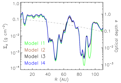
Figure 3: Dust surface densities (on the left Y axis) reconstructed from the iterative fitting process, and optical depth at a wavelength of 1.25 mm (on the right Y axis) for model I1, I2, I3 and I4. The dashed line shows the starting surface density used in the fitting loop: $\Sigma(R)\,{=}\,\Sigma_{0}\,(R/R_{\rm c})^{-\gamma}\,{\rm exp}[-(R/R_{\rm c})^{2-\gamma}]$ with $R_{\rm{c}}\,{=}\,90\,\rm{AU}$ and $\gamma\,{=}\,0.1$, see Sect. 3.3.

Along the disk minor axis, the change to the gap contrast as a function of $\Lambda$ is observed due to the effect of projection. Panel (d) of Figure 1 shows that models with a higher degree of dust settling produce more separate rings and deeper gaps, and vice versa. This fact is consistent with the findings reported by Pinte et al. [35]. Neither the D48 nor the D86 gap can be explained by model I1. Though both model I2 and I3 are consistent with the data of the D48 gap, only the former reproduces the D86 gap within the uncertainty, see Table 1.

The gas-to-dust scale height ratio $\Lambda$ has a strong impact on the brightness variation on the B67 and B100 rings. The well-mixed disk (model I1) shows two pronounced dips at $\phi\,{=}\,90^{\circ}$ and $\phi\,{=}\,270^{\circ}$, due to the difference in the optical depth ($\tau$) along the line of sight between $\phi\,{=}\,0^{\circ}$ (or $180^{\circ}$, major axis) and $\phi\,{=}\,90^{\circ}$ (or $270^{\circ}$, minor axis) [36]. Such a difference in $\tau$ decreases with increasing $\Lambda$. Consequently, the contrasts of “gaps” on the rings are reduced in more settled disks, see for instance model I3. Panels (e) and (f) of Figure 1 suggest that the degree of dust settling is different between B67 and B100. While B67 is close to a well-mixed situation, B100 favors a scenario in which large dust grains are well concentrated in the midplane.

4.2 Varying $\Lambda$ in the radial direction

Though the experiment under the assumption for a constant $\Lambda$ does not return a satisfactory solution, it provides clues to improve the model. The fitting results imply that the degree of dust settling changes with $R$. Therefore, we parameterize the ratio of gas-to-dust scale height with a piecewise function

$$\Lambda=\left\{\begin{array}[]{rcl}\Lambda{1}&:&{R\,{<}\,59\,\rm{AU}}\\ \Lambda{2}&:&{59\,\rm{AU}\,{\leq}\,R\,{<}\,78\,\rm{AU}}\\ \Lambda{3}&:&{78\,\rm{AU}\,{\leq}\,R\,{<}\,94\,\rm{AU}}\\ \Lambda{4}&:&{R\,{\geq}\,94\,\rm{AU}}.\\ \end{array}\right.$$ (5)

The boundaries of the four radial bins are chosen according to the locations and widths of the gaps and rings, see Sect. 2. We did not explore these borders in the fitting process. Using a piecewise form may have some artifacts in the boundaries. Nevertheless, how the gas-to-dust scale height ratio smoothly varies from one radial bin to another is difficult to be investigated, because it requires observational data at extremely high spatial resolutions that fully resolve the transition region between two adjacent bins. In the new model configuration, the ratios $\Lambda{2}$ and $\Lambda{4}$ are expected to play the dominated role in controlling the gap contrasts of the B67 and B100 rings, respectively. The gap contrasts of D48 and D86 are mainly influenced by a combination of $\Lambda{1}$ and $\Lambda{2}$, and a combination of $\Lambda{3}$ and $\Lambda{4}$, respectively. This is because the definition of contrasts of gaps on the major/minor axis is related to the brightnesses both in the gap and in its exterior ring, see Sect. 2.

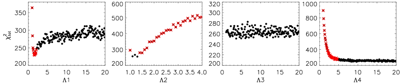
Figure 4: The $\chi_{\rm tot}^{2}$ distribution as a function of the gas-to-dust scale height ratio $\Lambda{1}$, $\Lambda{2}$, $\Lambda{3}$ and $\Lambda{4}$. The dots overlaid with a red cross refer to models that cannot reproduce all of the observed gap contrasts tabulated Table 1. Note that the $\chi_{\rm tot}^{2}\,{-}\,\Lambda{3}$ profile is flat, and most of the considered values for $\Lambda{3}$ are able to generate all of the observed gap contrasts. Therefore, $\Lambda{3}$ is basically not constrained.

The parameter space becomes $\left\{\Lambda{1},\,\Lambda{2},\,\Lambda{3},\,\Lambda{4},\,\Sigma_{d}\right\}$. To maintain self-consistency and independency, the time-consuming process for iterating $\Sigma_{d}$ has to be conducted for each of the sampled sets $\left\{\Lambda{1},\,\Lambda{2},\,\Lambda{3},\,\Lambda{4}\right\}$. Therefore, it is impractical to perform the parameter study using the Markov Chain Monte Carlo approach. Instead, the grid search method is invoked to finish the task. We first search for the optimum combination of $\Lambda{1}$ and $\Lambda{2}$, and then for that of $\Lambda{3}$ and $\Lambda{4}$. We sample 20 values for $\Lambda{1}$, which are logarithmically spaced from 1 and 20. Before the parameter study, we run many simulation tests, and find that models with $\Lambda{2}$ only slightly deviating from ${\sim}\,1.2$ are not able to generate gap contrasts of B67 comparable to the observation. Hence, for the sake of reducing the computational time and meanwhile being conservative, we consider 10 points for $\Lambda{2}$ from 1 to 4 in the logarithmic manner. At this stage, $\Lambda{3}$ and $\Lambda{4}$ are fixed to 2.6, i.e., the value of model I2. We run the iteration procedure for $\Sigma_{d}$ from scratch for each of the 200 different combinations of $\Lambda{1}$ and $\Lambda{2}$, and obtain 200 models. Then, we fix $\Lambda{1}$ and $\Lambda{2}$ to the values of the model with the lowest $\chi_{\rm tot}^{2}$. The exploration for $\Lambda{3}$ and $\Lambda{4}$ is similar. However, both parameters have the same grid points to those for $\Lambda{1}$, and therefore they form 400 different combinations.

The final best-fit model (model I4) features $\Lambda{1}\,{=}\,3.0$, $\Lambda{2}\,{=}\,1.2$, $\Lambda{3}\,{=}\,1.9$, $\Lambda{4}\,{=}\,16.3$, and $\chi_{\rm tot}^{2}\,{=}\,245$. Its dust surface density and millimeter optical depth are shown with the blue line in Figure 3. The model image and brightness profiles are compared with the observation in Figure 1. The gap contrasts and model parameters are summarized in Table 1 and 2, respectively. The best-fit model is able to explain all of the gap contrasts. We separately vary the gas-to-dust scale height ratios in each radial bin from their best-fit values with a step width of 0.1, and investigate how well the parameters are constrained. The variations of $\chi_{\rm tot}^{2}$ are shown in Figure 4. The dots overlaid with a red cross refer to models that cannot reproduce all of the observed gap contrasts within their errors. Therefore, we exclude them in the estimation of parameter uncertainties that are deduced from the models with $\chi_{\rm tot}^{2}$ less than 1.05 times the minimum $\chi_{\rm tot}^{2}$. For instance, all the models with $\Lambda 1\,{<}\,{\sim}2.2$ produce lower contrasts (i.e., ${<}\,0.92$) for the D48 gap measured on the disk minor axis than the observed value ($0.94\,{\pm}\,0.02$). Therefore, they are considered to be invalid although some of them have better $\chi^{2}_{\rm tot}$ than that of the best-fit model. The profiles of $\chi_{\rm tot}^{2}\,{-}\,\Lambda{1}$, $\chi_{\rm tot}^{2}\,{-}\,\Lambda{2}$ and $\chi_{\rm tot}^{2}\,{-}\,\Lambda{4}$ show a clear signature of getting the optimum solution, indicating that the gas-to-dust scale height ratios in the D48, B67 and B100 regions are well constrained. Their validity ranges are estimated to be [2.2, 3.3], [1.1, 1.3], and ${\geq}\,6.5$, respectively. The distribution of $\chi_{\rm tot}^{2}$ as a function of $\Lambda{3}$ is quite flat, and all the $\Lambda{3}$ values in the considered range can reproduce the data well. Hence, $\Lambda{3}$ is basically unconstrained.

5 Discussion

Using self-consistent radiative transfer models, we have placed constraints on the degree of dust settling by fitting the gap contrasts of the D48, B67, D86 and B100 features. Our results suggest a radially varying ratio of gas-to-dust scale height ratio in the HD 163296 disk. In this section, we compare our result with literature studies, and link the derived gas-to-dust scale height ratio to the turbulence strength in the HD 163296 disk.

5.1 Comparison of $\Lambda$ between different works

Ohashi et al. [78] found that the dust scale height is the key parameter for reproducing the azimuthal variation of the polarization pattern in the gaps. By analyzing the ALMA data of the 0.87 mm dust polarization from the HD 163296 disk, they constrained the dust scale height to be less than one-third the gas scale height for the D48 gap, and to be two-thirds the gas scale height for the D86 gap. Recently, Doi & Kataoka [36] showed that the azimuthal variation in the continuum along rings are sentitive to the degree of dust settling. Assuming that the disk is vertically isothermal with a fixed power-law temperature, they fit the DSHARP continuum data of the B67 and B100 rings, and inferred the ratio of gas-to-dust scale height to be 1.1 and ${>}\,9.5$ for the B67 and B100 ring, respectively. Figure 5 (upper panel) shows a comparison of $\Lambda$ between different works. The blue solid line refers to our best fit, whereas brown dots and green dots mark the results by Ohashi et al. [78] and Doi & Kataoka [36], respectively. As can be seen, our results are overall consistent with these literature values. However, as one step further, our analysis provides constraints on $\Lambda$ both for the ring and gap regions in the framework of self-consistent radiative transfer simulation.

The black dashed line in the upper panel of Figure 5 shows the dust scale height. In the inner ($R\,{<}\,60\,\rm{AU}$) or outermost ($R\,{>}\,94\,\rm{AU}$) regions, the millimeter dust disk is quite thin, with scale heights less than ${\sim}\,2\,\rm{AU}$. Disk regions in the vicinity of B67 have millimeter dust scale height of ${\sim}\,4\,\rm{AU}$. Disks, when viewed at high inclinations, have a specific advantage that the vertical extent of the emission layers can be directly constrained by spatially resolved images. Villenave et al. [79] presented ALMA continuum observations of 12 edge-on disks, at an angular resolution of ${\sim}\,0.1^{\prime\prime}$. A comparison between a set of radiative transfer models and the data indicates that at least three disks in their sample are consistent with a millimeter dust scale height of a few AU. Our inferred dust scale height for the HD 163296 disk, tilted to $46.7^{\circ}$, is comparable with those of the observed edge-on disks.

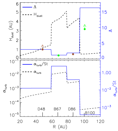
Figure 5: Upper panel: comparison of $\Lambda$ (on the right Y axis) between model I4 (blue solid line) and literature studies. The $\Lambda$ values by Ohashi et al. [78] and Doi & Kataoka [36] are indicated with brown dots and green dots, respectively. The black dashed curve shows the millimeter dust scale height (on the left Y axis) of model I4. Bottom panel: the $\alpha_{\rm turb}/{\rm St}$ ratio (blue solid line, on the right Y axis) and $\alpha_{\rm turb}$ (black dashed line, on the left Y axis) of model I4.

5.2 Comparison of $\alpha_{\rm turb}/\rm{St}$ and $\alpha_{\rm turb}$ between different works

Assuming an equilibrium between dust settling and vertical stirring by turbulent motions, the dust scale height and gas scale height follow the relation [80, 81]

$$H_{\rm dust}=H_{\rm gas}\left(1+\frac{\rm St}{\alpha_{\rm turb}}\frac{\rm 1+2\,St}{\rm 1+St}\right)^{-1/2},$$ (6)

where the Stokes number St is given by

$${\rm St}\,{=}\,\frac{\rho_{\rm grain}\bar{a}}{\Sigma_{\rm g}(R)}\frac{\pi}{2}.$$ (7)

The gas surface density $\Sigma_{\rm g}(R)\,{=}\,\Sigma_{0}\,(R/R_{\rm c})^{-\gamma}\,{\rm exp}[-(R/R_{\rm c})^{2-\gamma}]$ with $\Sigma_{0}\,{=}\,8.8\,\rm{g\,cm^{-2}}$, $R_{\rm{c}}\,{=}\,165\,\rm{AU}$ and $\gamma\,{=}\,0.8$, are constrained by high resolution multiple CO line observations [82]. Considering a grain size distribution like the one prescribed for the LGP, $\bar{a}$ stands for the representative grain size of dust that dominates the continuum emission at 1.25 mm. We check how the mass absorption coefficent $\kappa_{\rm abs}$ at 1.25 mm changes with $a$, and find that it peaks at $a\,{\sim}\,0.2\,\rm{mm}$. This value is close to the number given by $\lambda/2\pi$. Therefore, in our calculation of St, we took $\bar{a}\,{=}\,0.2\,\rm{mm}$.

Table 3: $\alpha_{\rm turb}/{\rm St}$ for the B67 and B100 ring from different studies.

Reference	B67 ring	B100 ring
Dullemond et al. [34]	0.33	$0.13\,{\sim}\,0.77$
Rosotti et al. [83]	0.23	0.04
Doi & Kataoka [36]	${>}\,2.4$	${<}\,0.011$
This work	$2.3_{-0.9}^{+2.5}$	$0.0038_{-0.0013}^{+0.02}$

The St value varies from ${\sim}\,10^{-5}$ in the inner disk to ${\sim}\,10^{-2}$ in the outer regions. Because St is much less than unity, Eq. 6 can be simplified as $H_{\rm dust}\,{=}\,H_{\rm gas}\left(1+\frac{\rm St}{\alpha_{\rm turb}}\right)^{-1/2}$. Therefore, the constrained $\Lambda$ directly translates into a ratio of $\alpha_{\rm turb}/\rm{St}$, which is shown with the blue solid line in the bottom panel of Figure 5. Based on different methodologies, other groups have derived the $\alpha_{\rm turb}/\rm{St}$ values for the B67 and B100 rings. For instance, Rosotti et al. [83] determined $\alpha_{\rm turb}/\rm{St}$ by measuring the deviation from Keplerian rotation of the gas in the proximity of the continuum peaks. Under an assumption that dust rings are caused by dust trapping in radial pressure bumps, Dullemond et al. [34] constrained $\alpha_{\rm turb}/{\rm St}$ by analyzing the widths of the dust rings. In Doi & Kataoka [36], the $\alpha_{\rm turb}/\rm{St}$ value was inferred by investigating the azimuthal intensity variation along dust rings. Table 3 summarizes the reported values together with our best-fit result. As can be seen, our result is well consistent with the values derived by Doi & Kataoka [36]. This is not surprising because the idea of constraning $\alpha_{\rm turb}/\rm{St}$ is the same. But, our methodology is more realistic, and data points not only on the rings but also along the major/minor axes are simultaneously taken into account in the analysis. We note that the best-fit $\alpha_{\rm turb}/{\rm St}$ for B67 is about one order of magnitude larger than those obtained in Dullemond et al. and Rosotti et al. There are several possibilities to explain such a difference. First, our methodology is sensitive to the strength of turbulent motions in the vertical direction, while the constraints by Dullemond et al. are more related to the radial diffusion of dust grains. Second, the B67 ring has a neighboring crescent, implying that the ring itself may not be perfectly axisymmetric, thus undermining the assumption of our modeling procedure. Third, if the gaps are indeed opened by planets [84, 85, 86], the B67 ring can be substantially stirred due to meridional gas flows. Numerical simulations have shown that massive planets can stir sub-millimeter-sized dust grains up to ${\sim}\,70\%$ of the gas scale height at the gap edges [87, 88]. For the B100 ring, we obtain a lower $\alpha_{\rm turb}/{\rm St}$ than that inferred by Dullemond et al. A lower turbulence in the vertical direction than in the radial direction can be explained under several physical scenarios, such as in dust feedback to turbulence [89], disk self-gravity [90], and radial (pseudo-)diffusion [91].

The black dashed line in the bottom panel of Figure 5 shows the derived turbulence strength. Except for the B67 ring, the disk has a turbulence level of $\alpha_{\rm turb}\,{<}\,3\times 10^{-3}$. Theoretical works have shown that pure hydrodynamic mechanisms or the magnetorotational instability suppressed by nonideal magnetohydrodynamic effects can generate similar turbulence levels in protoplanetary disks [92, 93, 4, 94, 95]. In the B67 ring, the turbulence is strong with $\alpha_{\rm turb}\,{\sim}\,1.2\,{\times}\,10^{-2}$.

Several studies have tried to measure turbulence in the HD 163296 disk through detailed analysis of gas line observations. Boneberg et al. [96] found that models with $\alpha_{\rm turb}\,{=}\,(0.1\,{-}\,6.3)\,{\times}\,10^{-3}$ match well with the ${\rm C^{18}O}\,J\,{=}\,2{-}1$ line profile within 90 AU of the disk. Based on CO isotopes and DCO⁺ line observations, Flaherty et al. [29, 30] derived the gas turbulence velocity in the disk, which is less than a few percent of the sound speed, corresponding to $\alpha_{\rm turb}\,{<}\,{\sim}\,3\,{\times}\,10^{-3}$. Our inferred value for $\alpha_{\rm turb}$, except for the B67 ring, is consistent with the results set by gas observations. The value of $\alpha_{\rm turb}$ for B67 from our modeling is larger than the upper limit in either Boneberg et al. or Flaherty et al. The discrepancy may be explained by two reasons. First, as demonstrated by our analysis, $\Lambda$, and therefore $\alpha_{\rm turb}$, may vary in the radial direction. The spatial resolution of gas line observations in Boneberg et al. and Flaherty et al. is ${\sim}\,0.5^{\prime\prime}$ that is 10 times worse than that of the DSHARP data. Consequently, their constraints on $\alpha_{\rm turb}$ represent a mean level of turbulence over a much broader range of radius than ours. Due to the beam smearing, low turbulence outside B67 results in a small $\alpha_{\rm turb}$ probed by the gas lines. Second, the turbulence strength we measure describes the role of dust stirring in the vertical direction. This may be different from the turbulence of gas motions. Recent numerical simulations of dust evolution start to use different $\alpha_{\rm turb}(s)$ for gas evolution, radial diffusion and vertical stirring [97].

Isella et al. [43] presented Band 6 ALMA observations of HD 163296 with a lower angular resolution than the DSHARP data, revealing three dust gaps at 60, 100, and 160 AU in the continuum as well as CO depletion in the middle and outer dust gaps. Liu et al. [98] investigated these gaps by performing 2D global hydrodynamic simulations of planet-disk interaction, and found that three half-Jovian-mass planets in a disk with effective viscosity being a function of radius can explain most of the observational features. Within $R\,{=}\,100\,\rm{AU}$, their model has a turbulence level of $\alpha_{\rm turb}\,{<}\,3\,{\times}\,10^{-4}$ that is weaker than ours. Such an inconsistency can be explained by the difference in the quality of data used in the analysis. As shown in the left column of Figure 3 in Liu et al. [98], the best-fit $\alpha_{\rm turb}$ is sensitive to how well the dust surface densities in the gap region are constrained. In the ALMA observation used by Liu et al. [98], the beam size is ${\sim}\,0.2^{\prime\prime}$ and the widths of the inner two gaps are narrower than ${\sim}\,0.27^{\prime\prime}$, indicating that the gaps are not fully resolved. However, our constraints are placed using the DSHARP data with four times better spatial resolution and sensitivity.

5.3 The effect of model assumptions on the results

The direct constraint from our radiative transfer analysis is on the gas-to-dust scale height ratio $\Lambda$. The scenario of dust settling that links $\Lambda$ and $\alpha_{\rm turb}$ is given by Eq. 6, and the relation is based on numerical simulations performed by Dubrulle et al. [54] and Youdin & Lithwick [80]. Models with more realistic physics on dust growth, sedimentation and radial mixing may alter the connection between dust and gas scale heights, therefore change the result.

To calculate the Stokes number characterizing the coupling between gas and dust, one needs to know the gas surface density. In our calculation, we take the result from Zhang et al. [82] who modeled the high resolution ALMA data of CO and its isotopologue lines. How well the CO molecular lines probe the underlying total gas surface density remains uncertain. Such a fact will not affect our constaints on $\Lambda$ from the continuum radiative transfer modeling, but it will cause uncertainties when inferring $\alpha_{\rm turb}$ from $\Lambda$, see Eq. 6.

6 Summary

Constraining the strength of turbulence plays a key role in building up our knowledge on disk evolution and planet formation. It is also crucial for running numerical models to interpret high-resolution ALMA observations. In this work, we took the HD 163296 disk as an example, and investigated in detail the millimeter gap contrast as a probe for turbulence level. With self-consistent radiative transfer modeling, we fit the gap contrasts measured for the D48, B67, D86 and B100 substructures that are spatially resolved by the DSHARP observation. We constrained the gas-to-dust scale height ratio $\Lambda$ to be $3.0_{-0.8}^{+0.3}$, $1.2_{-0.1}^{+0.1}$ and ${\geq}\,6.5$ for the D48, B67 and B100 regions. Our results show that the degree of dust settling varies with radius in the HD 163296 disk. The $\Lambda$ value for the D86 region is unconstrained due to the degeneracy between $\Lambda$ and the depth of surface density drops.

Based on the constrained gas-to-dust scale height ratio $\Lambda$, we estimate $\alpha_{\rm turb}/\rm{St}$ to be $2.3_{-0.9}^{+2.5}$ and $0.0038_{-0.0013}^{+0.02}$ for the B67 and B100 rings, respectively. These values are well consistent with those reported by Doi & Kataoka [36], but differ from the numbers inferred by Dullemond et al. [34] and Rosotti et al. [83]. The discrepancy may be due of the fact that our modeling is sentitive to the turbulence for vertical stirring of dust grains, while literature studies more likely reflect the turbulence for the radial diffusion of dust grains or the turbulent motion of gas species.

We calculate the turbulence level to be $\alpha_{\rm turb}\,{<}\,3\times 10^{-3}$ for the D48 and B100 regions, which agree well with the upper limit set by Boneberg et al. [96] and Flarherty et al. [30] from analyzing the width of gas lines. According to our analysis, the B67 ring has a strong turbulence strength of $\alpha_{\rm turb}\,{\sim}1.2\,{\times}\,10^{-2}$. Future multi-wavelength continuum observations with comparable spatial resolution to the DSHARP data are required to better constrain the degree of dust settling, and therefore the scale height of dust grains with different sizes. Higher resolution observations of multiple gas lines are pivotal to directly measure the turbulent motions, and confirm whether the strong turbulence in the local region of B67 inferred from our analysis is also seen with gas tracers.

We thank the anonymous referees for their constructive comments that highly improved the manuscript. YL acknowledges the financial support by the Natural Science Foundation of China (Grant No. 11973090), and the science research grants from the China Manned Space Project with NO. CMS-CSST-2021-B06. GHMB and MF acknowledge funding from the European Research Council (ERC) under the European Union’s Horizon 2020 research and innovation program (grant agreement No. 757957). GR acknowledges support from the Netherlands Organisation for Scientific Research (NWO, program number 016.Veni.192.233) and from an STFC Ernest Rutherford Fellowship (grant number ST/T003855/1). We thank Tilman Birnstiel, Guo Chen, Ke Zhang and Richard Teague for insightful discussions. We acknowledge the DSHARP team for making the calibrated CASA measurement sets, fiducial images, and the scripts used for calibration and image cleaning, available for the public. ALMA is a partnership of ESO (representing its member states), NSF and NINS, together with NRC, MOST and ASIAA, and KASI, in cooperation with the Republic of Chile. The Joint ALMA Observatory is operated by ESO, AUI/NRAO and NAOJ.

The authors declare that they have no conflict of interest.

Appendix Appendix More information about the SED models

In Sect. 3.4, we modeled the SED of the HD 163296 disk to constrain the maximum grain size ($a_{\rm max}$) for the LGP. Two models with $a_{\rm max}\,{=}\,1\,\rm{mm}$ (model S1) and $a_{\rm max}\,{=}\,1\,\rm{cm}$ (model S2) are shown in Figure 2. Because the SED analysis is not the key of this study, we do not present all the information in the main section.

The blue solid line in Figure 6 shows the gas scale height of model S2. The black solid line indicates the assumption made by Doi & Kataoka [36], which is also our initial choice for $H_{\rm gas}$ in the iteration (see Sect. 3.3). The black dashed line stands for a typical profile found from modeling the SEDs of T Tauri disks. Figure 7 shows the reconstructed surface densities ($\Sigma_{\rm d}$) for both models. As can be seen, they follow a similar pattern. However, the surface densities of model S2 are systematically larger than those of model S1. This is because the mass absorption coefficient at a wavelength of 1.25 mm for a dust grain population with $a_{\rm max}\,{=}\,1\,\rm{mm}$ is larger than that for a population of dust grains with $a_{\rm max}\,{=}\,1\,\rm{cm}$. Therefore, higher surface densities are required to fit the observed millimeter flux when $a_{\rm max}\,{=}\,1\,\rm{mm}$.

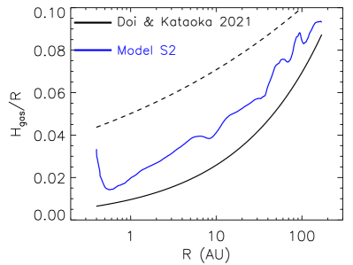
Figure 6: Gas scale height of the HD 163296 disk. The blue line refers to the result of model S2 (see Sect. 3.4), which is solved under the condition of vertical hydrostatic equilibrium. The black line show the scale height used in Doi & Kataoka [36]. The dashed curve, described as $H_{\rm gas}=10\,(R/100\,\rm{AU})^{1.15}$, is the typical disk geometry found from modeling the SEDs of T Tauri disks.

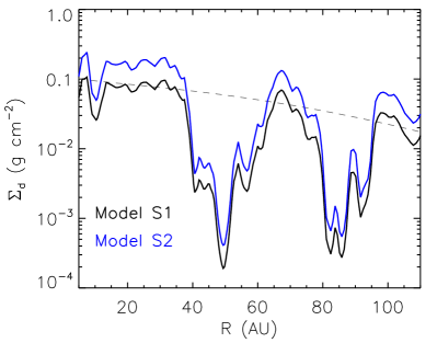
Figure 7: Dust surface densities of model S1 (black solid line) and model S2 (blue solid line). The grey dashed line represents the initial density profile used in the iteration process, see Sect. 3.3.

References

- [1] G. Lesur et al., arXiv e-prints (2022).
- [2] P. Goldreich and G. Schubert, ApJ150, 571 (1967).
- [3] K. Fricke, Zeitschrift für Astrophysik 68, 317 (1968).
- [4] M. Flock et al., ApJ850, 131 (2017).
- [5] W. Lyra, ApJ789, 77 (2014).
- [6] H. Klahr and A. Hubbard, ApJ788, 21 (2014).
- [7] P. S. Marcus et al., ApJ808, 87 (2015).
- [8] P. S. Marcus, S. Pei, C.-H. Jiang, and J. A. Barranco, ApJ833, 148 (2016).
- [9] S. A. Balbus and J. F. Hawley, ApJ376, 214 (1991).
- [10] S. A. Balbus, J. F. Hawley, and J. M. Stone, ApJ467, 76 (1996).
- [11] S. A. Balbus and J. F. Hawley, Reviews of Modern Physics 70, 1 (1998).
- [12] N. I. Shakura and R. A. Sunyaev, A&A24, 337 (1973).
- [13] J. E. Pringle, ARA&A19, 137 (1981).
- [14] T. Birnstiel, M. Fang, and A. Johansen, Space Science Reviews 205, 41 (2016).
- [15] W. Kley and R. P. Nelson, ARA&A50, 211 (2012).
- [16] H. Avenhaus et al., ApJ863, 44 (2018).
- [17] F. Long et al., ApJ869, 17 (2018).
- [18] S. M. Andrews et al., ApJ869, L41 (2018).
- [19] G. Dipierro et al., MNRAS475, 5296 (2018).
- [20] S. Zhang et al., ApJ869, L47 (2018).
- [21] Y. Liu et al., A&A622, A75 (2019).
- [22] P. Pinilla, M. Benisty, and T. Birnstiel, A&A545, A81 (2012).
- [23] M. Flock et al., A&A574, A68 (2015).
- [24] G. P. Rosotti, A. Juhasz, R. A. Booth, and C. J. Clarke, MNRAS459, 2790 (2016).
- [25] G. H. M. Bertrang et al., MNRAS474, 5105 (2018).
- [26] R. Dong, S. Li, E. Chiang, and H. Li, ApJ866, 110 (2018).
- [27] R. Teague et al., A&A592, A49 (2016).
- [28] S. Guilloteau et al., A&A548, A70 (2012).
- [29] K. M. Flaherty et al., ApJ813, 99 (2015).
- [30] K. M. Flaherty et al., ApJ843, 150 (2017).
- [31] R. Teague et al., ApJ864, 133 (2018).
- [32] K. Flaherty et al., ApJ895, 109 (2020).
- [33] C. P. Dullemond and A. B. T. Penzlin, A&A609, A50 (2018).
- [34] C. P. Dullemond et al., ApJ869, L46 (2018).
- [35] C. Pinte et al., ApJ816, 25 (2016).
- [36] K. Doi and A. Kataoka, ApJ912, 164 (2021).
- [37] Gaia Collaboration et al., A&A616, A1 (2018).
- [38] B. R. Setterholm et al., ApJ869, 164 (2018).
- [39] J. R. Fairlamb, R. D. Oudmaijer, I. Mendigutía, J. D. Ilee, and M. E. van den Ancker, MNRAS453, 976 (2015).
- [40] C. A. Grady et al., ApJ544, 895 (2000).
- [41] J. P. Wisniewski et al., ApJ682, 548 (2008).
- [42] G. A. Muro-Arena et al., A&A614, A24 (2018).
- [43] A. Isella et al., PhRvL 117, 251101 (2016).
- [44] S. Notsu et al., ApJ875, 96 (2019).
- [45] B. Lazareff et al., A&A599, A85 (2017).
- [46] J. Varga et al., A&A647, A56 (2021).
- [47] J. Huang et al., ApJ869, L42 (2018).
- [48] A. Isella et al., ApJ869, L49 (2018).
- [49] P. J. Rodenkirch, T. Rometsch, C. P. Dullemond, P. Weber, and W. Kley, A&A647, A174 (2021).
- [50] C. P. Dullemond et al. RADMC-3D: A multi-purpose radiative transfer tool Astrophysics Source Code Library, 2012.
- [51] R. Kurucz, 19 , (1994).
- [52] S. M. Andrews et al., ApJ732, 42 (2011).
- [53] Y. Liu, M. Flock, and M. Fang, Science China Physics, Mechanics, and Astronomy 65, 269511 (2022).
- [54] B. Dubrulle, G. Morfill, and M. Sterzik, Icarus114, 237 (1995).
- [55] C. P. Dullemond and C. Dominik, A&A421, 1075 (2004).
- [56] Y. Liu et al., A&A607, A74 (2017).
- [57] P. Woitke et al., A&A586, A103 (2016).
- [58] J. Dorschner, B. Begemann, T. Henning, C. Jaeger, and H. Mutschke, A&A300, 503 (1995).
- [59] V. G. Zubko, V. Mennella, L. Colangeli, and E. Bussoletti, MNRAS282, 1321 (1996).
- [60] D. Bruggeman, Ann. Phys. 416, 636 (1935).
- [61] M. Min, J. W. Hovenier, and A. de Koter, A&A432, 909 (2005).
- [62] C. P. Dullemond, A. Isella, S. M. Andrews, I. Skobleva, and N. Dzyurkevich, A&A633, A137 (2020).
- [63] L. Ricci et al., A&A512, A15 (2010).
- [64] L. Testi et al., in: Protostars and Planets VI, eds. H. Beuther, R. S. Klessen, C. P. Dullemond, and T. Henning, 2014, p. 339.
- [65] V. Mannings, MNRAS271, 587 (1994).
- [66] R. D. Oudmaijer et al., A&A379, 564 (2001).
- [67] R. M. Cutri et al., 2246 , (2003).
- [68] A. Isella et al., A&A469, 213 (2007).
- [69] D. Ishihara et al., A&A514, A1 (2010).
- [70] G. Sandell, D. A. Weintraub, and M. Hamidouche, ApJ727, 26 (2011).
- [71] R. M. Cutri and et al., 2328 , (2013).
- [72] N. Pascual et al., A&A586, A6 (2016).
- [73] A. Tripathi, S. M. Andrews, T. Birnstiel, and D. J. Wilner, ApJ845, 44 (2017).
- [74] G. Guidi et al., arXiv e-prints (2022).
- [75] A. Li and B. T. Draine, ApJ554, 778 (2001).
- [76] C. P. Dullemond, D. Hollenbach, I. Kamp, and P. D’Alessio, in: Protostars and Planets V, eds. B. Reipurth, D. Jewitt, and K. Keil, 2007, p. 555.
- [77] P. M. Harvey et al., ApJ755, 67 (2012).
- [78] S. Ohashi and A. Kataoka, ApJ886, 103 (2019).
- [79] M. Villenave et al., A&A642, A164 (2020).
- [80] A. N. Youdin and Y. Lithwick, Icarus192, 588 (2007).
- [81] T. Birnstiel, C. P. Dullemond, and F. Brauer, A&A513, A79 (2010).
- [82] K. Zhang et al., ApJS257, 5 (2021).
- [83] G. P. Rosotti, R. Teague, C. Dullemond, R. A. Booth, and C. J. Clarke, MNRAS495, 173 (2020).
- [84] C. Pinte et al., ApJ860, L13 (2018).
- [85] R. Teague, J. Bae, E. A. Bergin, T. Birnstiel, and D. Foreman-Mackey, ApJ860, L12 (2018).
- [86] R. Teague et al., ApJS257, 18 (2021).
- [87] J. Bi, M.-K. Lin, and R. Dong, ApJ912, 107 (2021).
- [88] F. Binkert, J. Szulágyi, and T. Birnstiel, MNRAS506, 5969 (2021).
- [89] Z. Xu and X.-N. Bai, arXiv e-prints (2022).
- [90] H. Baehr and Z. Zhu, ApJ909, 136 (2021).
- [91] Z. Hu and X.-N. Bai, MNRAS503, 162 (2021).
- [92] X.-N. Bai and J. M. Stone, ApJ736, 144 (2011).
- [93] X.-N. Bai, ApJ798, 84 (2015).
- [94] C. Cui and X.-N. Bai, ApJ891, 30 (2020).
- [95] C. Cui and X.-N. Bai, MNRAS507, 1106 (2021).
- [96] D. M. Boneberg, O. Panić, T. J. Haworth, C. J. Clarke, and M. Min, MNRAS461, 385 (2016).
- [97] P. Pinilla, C. T. Lenz, and S. M. Stammler, A&A645, A70 (2021).
- [98] S.-F. Liu, S. Jin, S. Li, A. Isella, and H. Li, ApJ857, 87 (2018).