Non-Abelian Fusion, Shrinking and Quantum Dimensions of Abelian Gauge Fluxes

Abstract

Braiding and fusion rules of topological excitations are indispensable topological invariants in topological quantum computation and topological orders. While excitations in 2D are always particle-like anyons, those in 3D incorporate not only particles but also loops—spatially nonlocal objects—making it novel and challenging to study topological invariants in higher dimensions. While 2D fusion rules have been well understood from bulk Chern-Simons field theory and edge conformal field theory, it is yet to be thoroughly explored for 3D fusion rules from higher dimensional bulk topological field theory. Here, we perform a field-theoretical study on (i) how loops that carry Abelian gauge fluxes fuse and (ii) how loops are shrunk into particles in the path integral, which generates fusion rules, loop-shrinking rules, and descendent invariants, e.g., quantum dimensions. We first assign a gauge-invariant Wilson operator to each excitation and determine the number of distinct excitations through equivalence classes of Wilson operators. Then, we adiabatically shift two Wilson operators together to observe how they fuse and are split in the path integral; despite the Abelian nature of the gauge fluxes carried by loops, their fusions may be of non-Abelian nature. Meanwhile, we adiabatically deform world-sheets of unknotted loops into world-lines and examine the shrinking outcomes; we find that the resulting loop-shrinking rules are algebraically consistent to fusion rules. Interestingly, fusing a pair of loop and anti-loop may generate multiple vacua, but fusing a pair of anyon and anti-anyon in 2D has one vacuum only. By establishing a field-theoretical ground for fusion and shrinking in 3D, this work leaves intriguing directions for future exploration, e.g., symmetry enrichment, quantum gates, and physics of braided monoidal 2-category of 2-group.

I Introduction

Topological order and topological excitations.—Topologically ordered phases which are beyond the paradigm of symmetry-breaking theory have attracted lots of attentions for years (Wen, 2019, 2015; Levin and Wen, 2005; Wen, 2017a; Hartnoll et al., 2021; Zeng et al., 2015) from not only condensed matter physics, but also high-energy physics, quantum information science, and mathematical physics. Experimentally confirmed by the fractional quantum Hall effect (FQHE), topological order cannot be characterized by any local order parameters. At low energies, topological quantum field theory (TQFT) is utilized as the effective field theory to describe topologically ordered phases. In addition, inspired by quantum information science, topological order of a gapped many-body system is tightly connected to the pattern of long-range entanglement Zeng et al. (2015). Recently, the algebraic theory for 2D topological orders has also been explored deeply, making it intriguing to make joint efforts in condensed matter physics and mathematical category theory, see, e.g., concise introductory materials in Refs. (Barkeshli et al., 2019).

Topological excitations are essential ingredients of topologically ordered phases. In absence of any symmetry-breaking order parameters, the topological properties, such as fusion and braiding statistics of topological excitations constitute the key observables of topological orders and also important processes in Topological Quantum Computation (TQC) Nayak et al. (2008). Analogous to quasi-particles in solid-state physics, topological excitations are collective phenomena and can be created as localized energy lump above the ground state. In $2$D space, topological excitations are point-like particle excitations, e.g., the anyon excitations in FQHE. In $3$D space, topological excitations incorporate not only particle excitations but also loop excitations that are spatially nonlocal. Moreover, a loop excitation can also be decorated by a particle excitation, i.e., a particle excitation is attached to a loop excitation, named decorated loop (see Fig. 2). For those loop excitations not decorated by particle excitations, we call them pure loops. If we move forward to $4$D space, we would find that topological excitations there include $2$-dimensional closed-surface-like membrane excitations (Zhang and Ye, 2022; Chen et al., 2021).

Braiding statistics.—Let us first review braiding statistics of topological excitations. During a braiding process of particles and loops, an adiabatic quantum phase is accumulated which is proportional to the linking invariant of the link formed by world-lines of particles and world-sheets of loops. For the braiding processes in $4$D space, the emergence of world-volumes of membrane excitations generates a large variety of exotic linking invariants (Zhang and Ye, 2022). These adiabatic quantum phases are called braiding phases, serving as an important data set to characterize topological order. TQFT, as the low-energy effective theory of topological order, provides us a quantitative approach to braiding phase (Witten, 1989). For example, the braiding phases of anyons in $2$D space are captured by the $\left(2+1\right)$D Chern-Simons theory ($\sim tr(A\wedge dA+\frac{2}{3}A\wedge A\wedge A)$) (Witten, 1989; Wen, 2004, 2015; Blok and Wen, 1990). In $3$D space, braiding processes involve particles and loops. If we consider a discrete gauge group $G=\prod_{i}\mathbb{Z}_{N_{i}}$, all particles and loops can be labeled by periodic gauge charges and gauge fluxes respectively. The braiding processes can be divided into three classes: particle-loop braiding (Hansson et al., 2004; Aharonov and Bohm, 1959; Preskill and Krauss, 1990; Alford and Wilczek, 1989; Krauss and Wilczek, 1989; Alford et al., 1992), multi-loop braiding (Wang and Levin, 2014; Wang et al., 2015; Putrov et al., 2017; Ye and Gu, 2016; Ning et al., 2016; Wang and Wen, 2015; Ye, 2018; Ning et al., 2022; Wang et al., 2019; Jian and Qi, 2014; Jiang et al., 2014; Wang et al., 2016; Wan et al., 2015; Kapustin and Thorngren, 2014; Chen et al., 2016; Wang et al., 2016; Tiwari et al., 2017; Peng, 2020; Han et al., 2019), and particle-loop-loop braiding [i.e., Borromean rings (BR) braiding] (Chan et al., 2018). In each class, there are different braiding phases depending on different assignments of gauge group. The TQFTs describing these braiding processes are expressed as the combination of a multi-component $BF$ term (Horowitz and Srednicki, 1990; Baez et al., 2007; Bullivant et al., 2019; Ye et al., 2016, 2017; Cho and Moore, 2011) with twisted terms. The $BF$ term in $\left(3+1\right)$D is written as $B\wedge dA$ where $B$ and $A$ are $2$- and $1$-form $\mathbb{U}\left(1\right)$ gauge fields respectively. For multi-loop braiding, the twisted terms $AAdA$ and $AAAA$ ($\wedge$ is omitted)  (Putrov et al., 2017) correspond to $3$-loop and $4$-loop braidings, respectively. For particle-loop-loop braiding (BR braiding, see Fig. 1), the twisted term is $AAB$ (Chan et al., 2018). If we consider a topologically ordered system that supports particle-loop and/or multi-loop braiding, the TQFT is consistent with the Dijkgraaf-Witten (DW) cohomological classification $\mathcal{H}^{4}\left(G,U\left(1\right)\right)$ for gauge group $G$. Nevertheless, once we demand the system to support BR braiding as well, some multi-loop braidings would be excluded in the sense that no legitimate DW TQFT describing all these braidings can be constructed. Such incompatibility between BR braiding and multi-loop braiding can be traced back to the requirement of gauge invariance for TQFT (Zhang and Ye, 2021). For the purpose of this paper, we denote a system is equipped with Borromean rings topological order (BR topological order) if it supports BR braiding.

Fusion rules and loop-shrinking rules.—Fusion rules of topological excitations form another important set of topological invariants for 3D topological order. Pictorially, the fusion of two topological excitations is to adiabatically bring them together in space and the combined object behaves like another topological excitation. To be more precise, each topological excitation $\mathsf{e}_{i}$ corresponds to a fusion space $\mathcal{V}\left(M_{d};\mathsf{e}_{i}\right)$ where $M_{d}$ is the spatial manifold supporting all topological excitations (Wen, 2015). The bases of $\mathcal{V}\left(M^{d};\mathsf{e}_{i}\right)$ are degenerate ground states of $H+\delta H_{i}$ with $H_{i}$ is non-zero only near the location of $\mathsf{e}_{i}$. If the dimension of $\mathcal{V}\left(M_{d};\mathsf{e}_{i}\right)$ cannot be altered by any local perturbation near the location of $\mathsf{e}_{i}$, the type of $\mathsf{e}_{i}$ is simple. Otherwise, the type of $\mathsf{e}_{i}$ is composite. The fusion space of a composite topological excitation can be decomposed as a direct sum of that of other simple topological excitations. The fusion of two simple topological excitations, e.g., $\mathsf{a}$ and $\mathsf{b}$, corresponds to the direct product of their fusion space: $\mathcal{V}\left(M_{d};\mathsf{a}\right)\otimes\mathcal{V}\left(M_{d};\mathsf{b}\right)$. The resulting fusion space may correspond to another simple excitation, e.g., $\mathsf{c}$, and this fusion is called Abelian fusion: $\mathcal{V}\left(M_{d};\mathsf{a}\right)\otimes\mathcal{V}\left(M_{d};\mathsf{b}\right)=\mathcal{V}\left(M_{d};\mathsf{c}\right)$. It may also correspond to a direct sum of fusion spaces of multiple simple excitations, e.g., $\mathcal{V}\left(M_{d};\mathsf{a}\right)\otimes\mathcal{V}\left(M_{d};\mathsf{b}\right)=\mathcal{V}\left(M_{d};\mathsf{d}\right)\oplus\mathcal{V}\left(M_{d};\mathsf{f}\right)$, and such fusion is called non-Abelian fusion. The fusion rules are just simplified notations for the previous algebraic relations: $\mathsf{a}\otimes\mathsf{b}=\mathsf{c}$ or $\mathsf{a}\otimes\mathsf{b}=\mathsf{d}\oplus\mathsf{f}$. In a more general setting, the fusion rule of two simple topological excitations can be given by $\mathsf{a}\otimes\mathsf{b}=\oplus_{i}N_{\mathsf{e}_{i}}^{\mathsf{a}\mathsf{b}}\mathsf{e}_{i}$ where $N_{\mathsf{e}_{i}}^{\mathsf{a}\mathsf{b}}$ is a non-negative integer and the type of $\mathsf{e}_{i}$ is simple. In this paper, unless otherwise specified, “excitations” are always of simple type.

In the literature, fusion in $2$D topological orders has been studied extensively from exactly solvable models, field theory, to mathematical foundation. For example, fusion rules of anyons are encoded in the mathematical concept of unitary fusion tensor categories (Turaev, 2016; Bakalov and Kirillov, 2001). On the other hand, just like the role of loops in exotic braiding statistics reviewed above, loop excitations that are entirely absent in $2$D topological orders, are also expected to contribute nontrivial fusion rules in 3D topological orders. The nature of non-locality of loop excitations may significantly complicate but meanwhile significantly enrich the analysis of fusion rules (see, e.g., the cartoons in Figs. 3, 4). Firstly, combinatorially, we need to analyze fusions of (i) two particles, (ii) two loops, and (iii) one particle plus one loop. Secondly, as loops can be either pure loops or decorated loops as reviewed above, the resulting fusion data are expected to be further enriched. Thirdly, one can also consider self-knotted or mutually linked loops (see, e.g., Fig. 1 of Ref. Wen et al. (2018)) and study their fusion rules. Fourthly, while there have been intensive discussions in realization and manipulation of Majorana zero modes (see, e.g., incomplete reference list: Refs. Ivanov (2001); Beenakker et al. (2019); Stone and Chung (2006)), it will be of great interests to explore how to implement fusion rules of loop excitations (“loop-like errors/defects” by following nomenclature in quantum information science) in TQC gates of stabilizer codes. All in all, fusion rules for loops in 3D topological orders deserve a thorough study from various aspects.

Besides, the presence of loops provides us with another indispensable topological invariants—loop-shrinking rules. A loop excitation, if it is unknotted, can be smoothly shrunk to a point (see Fig. 5). Notice that this process is apparently meaningless for particle excitations that are already point-like, so the exploration of such topological invariants should be at least starting from 3D topological orders. Interestingly, such a shrinking process can be alternatively understood as the consequence of observing a loop when an observer stands far away from the loop such that the loop “looks like” a point. It is curious to ask what is the consequence of such a loop-shrinking operation? How can we analytically describe this process, e.g., by means of field theory? Can we obtain another set of meaningful topological invariants from such an operation? To answer questions of such kinds, it is highly worthwhile to conduct an in-depth study into the outcomes of such a loop-shrinking operation, which are encoded in the loop-shrinking rules that are lacking in $2$D topological orders. All in all, we expect that the presence of non-local loops in 3D topological orders will lead to not only nontrivial braiding statistics as studied before but also fruitful quantum phenomena encoded in fusion rules and loop-shrinking rules. This line of efforts will be of great help for deeply understanding topological orders of all dimensions, theoretically developing TQC for all dimensions, and proposing experimental manipulation of braiding, fusion, and shrinking of non-local topological excitations in the future.

From the tradition of condensed matter physics and also by following the spirit of renormalization group and universality, it is always vital to explore the long-distance low-energy effective field theory of underlying phases of matter, and further ask how to systematically define and compute observables from such effective field theories. It has been known that Ginzburg-Landau perturbative field theories are used to describe symmetry-breaking phases, but for topological orders, topological field theories are the correct field-theoretical language. While it has been well established that the topological invariants (e.g., fusion rules and braiding) of 2D topological orders can be systematically extracted from $(2+1)$D bulk Chern-Simons field theory as well as edge CFT (conformal field theory), it is still yet to be thoroughly explored for fusion rules and loop-shrinking rules of 3D topological orders from $(3+1)$D field theories that are generally TQFT of certain types. Thus, it is important to perform such a topological-field-theoretical study.

Motivated by, but not limited to, above discussions, in this paper, we aim to perform a topological-field-theoretical study on fusion rules and loop-shrinking rules of $3$D topological orders when all loops carry Abelian gauge fluxes. Specially, we start with the BR topological order with Abelian gauge group $G=\left(\mathbb{Z}_{N}\right)^{3}$. In details, we first construct and classify topologically distinct Wilson operators for all types of particles and loops by means of path-integral quantization. Then, the number of topological excitations is just the number of Wilson operators, collected in Tables 1, 2, and 3. Next, we study fusion rules in terms of path integral. In practice, we spatially fuse two Wilson operators together, which leads to nontrivial splitting in the path integral formalism. We collect all fusion coefficients in Table 4, where there exist non-Abelian fusion processes despite the Abelian nature of the gauge fluxes carried by loops. From the fusion coefficients, we can also extract quantum dimensions for all excitations, as collected in Table 5. Then, we compute shrinking rules for loop excitations (see Table 6), i.e., the process of shrinking an unknotted loop excitation into particles, which are found to be algebraically consistent with the fusion rules, and are critical in establishing an anomaly-free topological order. We also find an interesting phenomenon that fusing a loop and anti-loop may generate more than one vacuum, which is different from 2D topological orders where fusing a pair of particle and antiparticle has one vacuum only. At last, we generalize the above analysis to topological orders with gauge group $G=\prod_{i}^{n}\mathbb{Z}_{N_{i}}$ ($n=1,2,3$) where various interesting braiding statistics can be realized. This work establishes a continuum field-theoretical ground for fusion, shrinking and quantum dimensions in 3D TO, and also future explorations.

Outline.—This paper is organized as follows. In Sec. II, we review the TQFT action of BR topological order and construct Wilson operators for topological excitations. The number of topological excitations is consistent with that computed from a lattice cocycle model. In Sec. III, fusion rules of excitations are derived via Wilson operators and path integral. Besides, the shrinking rules for loops are also studied, which shows consistency with the fusion data. In Sec. IV, the relation between fusion rules and combinations of compatible braiding processes is studied, which generalizes the above analysis to topological orders with gauge group $G=\prod_{i}^{n}\mathbb{Z}_{N_{i}}$ ($n=1,2,3$). Discussion and outlook are given in Sec. V. Technical details are collected in the Appendices.

II Wilson operators for topological excitations

In order to study fusion rules in TQFT, we first need to express topological excitations in the field-theoretical formalism. For each topological excitation carrying a specific amount of gauge charges and gauge fluxes, it is uniquely represented by a Wilson operator that is invariant under gauge transformations. In this section, we begin with reviewing the TQFT action for BR topological order with gauge group $G=\prod_{i=1}^{3}\mathbb{Z}_{N_{i}}$. Then, by considering $N_{1}=N_{2}=N_{3}=2$ as a typical example, we construct Wilson operators for topological excitations, i.e., particles, pure loops, and decorated loops. In this case, there are $2^{3}\times 2^{3}=64$ different combinations of gauge charges and gauge fluxes, which seems to indicate that there are $64$ different topological excitations, i.e., Wilson operators. Nevertheless, we find that some Wilson operators have the same correlation function with an arbitrary operator. In this sense, such Wilson operators belong to the same equivalence class. Finally, among $64$ possible Wilson operators we find only $19$ nonequivalent ones, i.e., $19$ essentially different topological excitations, for BR topological order with $G=\left(\mathbb{Z}_{2}\right)^{3}$. These $19$ nonequivalent Wilson operators corresponding to $19$ topological excitations are listed in Table. 1 (particles), Table. 2 (pure loops) , and Table. 3 (decorated loops) which are the cornerstone of fusion rules in Sec. III.

II.1 TQFT action for BR topological order

BR topological order (Chan et al., 2018) is featured with a special braiding process of one particle and two loops which carry gauge charge or fluxes from three different gauge subgroups. In this braiding process, the spatial trajectory of particle and two loops form Borromean rings (or general Brunnian link) in $3$D space, as shown in Fig. 1. The braiding phase of this process is proportional to the Milnor’s triple linking number (Chan et al., 2018; Milnor, 1954; Mellor and Melvin, 2003).

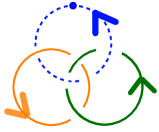
Figure 1: Illustration of Borromean rings braiding that is realized in the topological order described by Eq. (1). In this braiding process, Borromean rings is formed by the spatial trajectory of the particle (blue) and two loops (orange and green).

This Borromean rings braiding cannot be classified by cohomology group $\mathcal{H}^{4}\left(G,U\left(1\right)\right)$ for gauge group $G$. The latter is applicable only for particle-loop braidings and multi-loop braidings. In addition, a Borromean rings braiding is compatible with specific multi-loop braidings only for a given gauge group $G$. In other words, a legitimate DW TQFT can only describe Borromean rings braiding and some, but not all, of multi-loop braidings simultaneously. By legitimacy we mean that the DW TQFT is a theory with well-defined gauge transformations (Zhang and Ye, 2021).

In the following, we consider gauge group $G=\prod_{i=1}^{3}\mathbb{Z}_{N_{i}}$. The action for BR topological order is

$$S=\int\sum_{i=1}^{3}\frac{N_{i}}{2\pi}B^{i}dA^{i}+qA^{1}A^{2}B^{3},$$ (1)

where $A^{i}$ and $B^{i}$are $1$- and $2$-form $\mathbb{U}\left(1\right)$ gauge fields respectively. The coefficient $q=\frac{pN_{1}N_{2}N_{3}}{\left(2\pi\right)^{2}N_{123}}$ with $p\in\mathbb{Z}_{N_{123}}$, where $N_{123}$ is the greatest common divisor (GCD) of $N_{1}$, $N_{2}$ and $N_{3}$. The quantization of $q$ is the result of the large gauge invariance. In action (1), $B^{1}$, $B^{2}$, and $A^{3}$ serve as the Lagrange multipliers which locally enforce the flat-connection conditions: $dA^{1}=0$, $dA^{2}=0$, and $dB^{3}=0$. The gauge transformations for the action (1) are given by

$$A^{1}\rightarrow A^{1}+d\chi^{1},$$ (2)

$$A^{2}\rightarrow A^{2}+d\chi^{2},$$ (3)

$$A^{3}\rightarrow A^{3}+d\chi^{3}+X^{3},$$ (4)

$$B^{1}\rightarrow B^{1}+dV^{1}+Y^{1},$$ (5)

$$B^{2}\rightarrow B^{2}+dV^{2}+Y^{2},$$ (6)

$$B^{3}\rightarrow B^{3}+dV^{3},$$ (7)

with nontrivial shifts

$$X^{3}= -\frac{2\pi q}{N_{3}}\left(\chi^{1}A^{2}+\frac{1}{2}\chi^{1}d\chi^{2}\right)$$

$$+\frac{2\pi q}{N_{3}}\left(\chi^{2}A^{1}+\frac{1}{2}\chi^{2}d\chi^{1}\right),$$ (8)

$$Y^{1}= -\frac{2\pi q}{N_{1}}\left(\chi^{2}B^{3}-A^{2}V^{3}+\chi^{2}dV^{3}\right),$$ (9)

$$Y^{2}= \frac{2\pi q}{N_{2}}\left(\chi^{1}B^{3}-A^{1}V^{3}+\chi^{1}dV^{3}\right),$$ (10)

where $\chi^{i}$ and $V^{i}$ are respectively $0$-form and $1$-form gauge parameters with $\int d\chi^{i}\in 2\pi\mathbb{Z}$ and $\int dV^{i}\in 2\pi\mathbb{Z}$.

II.2 $G=\left(\mathbb{Z}_{2}\right)^{3}$: Operators for topological excitations and their equivalence classes

Since our TQFT action (1) is a gauge theory, it is expected that the operators for topological excitations are gauge-invariant. Notice that the gauge group is $G=\prod_{i=1}^{3}\mathbb{Z}_{N_{i}}$, the topological excitations include particles carrying $\mathbb{Z}_{N_{i}}$ gauge charges, loops carrying $\mathbb{Z}_{N_{i}}$ gauge flux only (pure loop), and loops simultaneously carrying $\mathbb{Z}_{N_{i}}$ gauge flux and $\mathbb{Z}_{N_{j}}$ gauge charge (decorated loops; $i$ and $j$ can be same or different), as illustrated in Fig. 2. The $\mathbb{Z}_{N_{i}}$ gauge charges and $\mathbb{Z}_{N_{i}}$ gauge fluxes are group representations and conjugacy classes of $\mathbb{Z}_{N_{i}}$ gauge subgroup. Only simple (see Introduction) topological excitations are considered in this paper. In this section, we explain how to label topological excitations by Wilson operators. Furthermore, we show that some topological excitations are equivalent in the path integral formalism, which leads to the notion of equivalence class among Wilson operators.

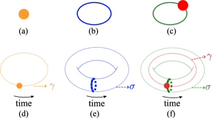
Figure 2: (a) Particle excitation carrying gauge charge in $3$D space. (b) Pure loop excitation carrying gauge flux in $3$D space. In this paper, we only consider loop excitations which are unknotted and thus can be deformed to $S^{1}$ smoothly. (c) Decorated loop carrying gauge flux and charge simultaneously. A decorated loop can be viewed as a pure loop with a particle attached to it. This particle (red solid circle) can be located at any position on the loop. (d) The closed world-line of particle denoted by $\gamma$. (e) The closed world-sheet of pure loop denoted by $\sigma$. (f) The space-time trajectories of decorated loop. In $\left(3+1\right)$D spacetime, $\sigma$ is a torus and $\gamma$ is a closed curve that is not self-knotted. For the particle attached to a loop excitation, its world-line $\gamma$ would be the non-contractible path on $\sigma$ circling along the time direction.

First, if we consider a particle with one unit of $\mathbb{Z}_{N_{1}}$ gauge charge (a $\mathbb{Z}_{N_{1}}$ particle), we can use the following operator to represent it:

$$\mathsf{P}_{100}=\exp\left({\rm i}\int_{\gamma}A^{1}\right),$$ (11)

where the closed $1$-dimensional $\gamma$ can be understood as the closed world-line of particle in $\left(3+1\right)$D spacetime. $\gamma$ is a closed curve in $\left(3+1\right)$D spacetime and can be deformed to $S^{1}$ smoothly, as shown in Fig. 2. The capital letter $\mathsf{P}$ stands for particle excitation and the subscript $n_{1}n_{2}n_{3}$ of $\mathsf{P}_{n_{1}n_{2}n_{3}}$ denotes the number of $\mathbb{Z}_{N_{1}}$, $\mathbb{Z}_{N_{2}}$, and $\mathbb{Z}_{N_{3}}$ gauge charges respectively. For instance, the subscript of $\mathsf{P}_{100}$ denotes that this particle excitation carries one unit of $\mathbb{Z}_{N_{1}}$ gauge charge and vanishing $\mathbb{Z}_{N_{2}}$ or $\mathbb{Z}_{N_{3}}$ gauge charge. The anti-particle of $\mathsf{P}_{100}$ is represented by

$$\bar{\mathsf{P}}_{100}=\mathsf{P}_{\left(-1\right)00}=\exp\left(-{\rm i}\int_{\gamma}A^{1}\right).$$ (12)

For simplicity, we let the gauge group to be $G=\left(\mathbb{Z}_{2}\right)^{3}$, i.e., $N_{1}=N_{2}=N_{3}=2$. We consider

$$\left\langle\mathsf{P}_{\left(-1\right)00}\right\rangle= \frac{1}{\mathcal{Z}}\int\mathcal{D}\left[A^{i}\right]\mathcal{D}\left[B^{i}\right]\exp\left({\rm i}S\right)$$

$$\times\exp\left(-{\rm i}\int_{\gamma}A^{1}\right),$$ (13)

where $\mathcal{Z}=\int\mathcal{D}\left[A^{i}\right]\mathcal{D}\left[B^{i}\right]\exp\left({\rm i}S\right)$ is the partition function. Integrating out $B^{1}$ leads to the constraint

$$\oint A^{1}=\frac{2\pi m_{1}}{N_{1}}=\frac{2\pi m_{1}}{2},m_{1}\in\mathbb{Z}.$$ (14)

This constraint implies $\exp\left({\rm i}2\int_{\gamma}A^{1}\right)=1$. With this fact, the expectation value of $\mathsf{P}_{\left(-1\right)00}$ can be written as

$$\left\langle\mathsf{P}_{\left(-1\right)00}\right\rangle= \frac{1}{\mathcal{Z}}\int\mathcal{D}\left[A^{i}\right]\mathcal{D}\left[B^{i}\right]\exp\left({\rm i}S\right)$$

$$\times\exp\left(-{\rm i}\int_{\gamma}A^{1}\right)\times\exp\left({\rm i}2\int_{\gamma}A^{1}\right)$$

$$= \left\langle\mathsf{P}_{100}\right\rangle.$$ (15)

In the sense of path integral, we can see that the anti-particle of $\mathsf{P}_{100}$ is itself when $G=\left(\mathbb{Z}_{2}\right)^{3}$. This result is easy to understand since the particle carries gauge charge of cyclic $\mathbb{Z}_{2}$ group.

Next, we consider a pure loop carrying one unit of $\mathbb{Z}_{N_{3}}$ flux, denoted as $\mathbb{Z}_{N_{3}}$-loop for simplicity. The corresponding operator is

$$\mathsf{L}_{001}=\exp\left({\rm i}\int_{\sigma}B^{3}\right),$$ (16)

where $\sigma$ is a closed $2$-dimensional surface as the closed world-sheet of a loop. In details, $\sigma$ is a $2$-torus formed by circling the loop along the time direction, as shown in Fig. 2. The letter $\mathsf{L}$ stands for loop excitations. For pure loop excitations, the subscript denotes the gauge fluxes carried by the loop. Similarly, for a pure loop carrying one (mod $2$) unit of $\mathbb{Z}_{2}$ flux, its anti-loop is itself, e.g., $\bar{l}_{001}=l_{00\left(-1\right)}=\exp\left({\rm i}\int_{\sigma}B^{3}\right)$.

Last, we consider a decorated loop [see Fig. 2(c)]. For instance, a $\mathbb{Z}_{N_{3}}$-loop decorated by a $\mathbb{Z}_{N_{1}}$-particle is represented by

$$\mathsf{L}_{001}^{100}=\exp\left({\rm i}\int_{\sigma}B^{3}+{\rm i}\int_{\gamma}A^{1}\right).$$ (17)

For decorated loop excitations, the superscript (e.g., “$100$” in $\mathsf{L}_{001}^{100}$) denotes the charge decoration, i.e., the gauge charges carried by the particle attached to the loop. Such decoration of particle on a loop requires that the particle’s world-line $\gamma$ lies on the loop’s world-sheet $\sigma$. This requirement is reasonable: imagine a loop moving in $\left(3+1\right)$D spacetime, the decorated particle also moves together with the loop, thus its world-line becomes a non-contractible path on the world-sheet of loop, as illustrated in Fig. 2.

One may notice that in gauge transformations (7), some gauge fields transform by a shift term, i.e., $X^{3}$, $Y^{1}$, or $Y^{2}$. These shift terms indicate that the gauge-invariant operators of these gauge fields needs to be treated carefully. For example, we consider the operator for $B^{1}$ gauge field which corresponds to a pure loop carrying $\mathbb{Z}_{N_{1}}$flux:

$$\mathsf{L}_{100}$$

$$= 2\exp\left[{\rm i}\int_{\sigma}B^{1}+\frac{1}{2}\frac{2\pi q}{N_{1}}\left(d^{-1}A^{2}B^{3}+d^{-1}B^{3}A^{2}\right)\right]$$

$$\times\delta\left(\int_{c}A^{2}\right)\delta\left(\int_{\sigma}B^{3}\right)$$ (18)

with $d^{-1}A^{2}=\int_{\left[a,b\right]\in c}A^{2}$ and $d^{-1}B^{3}=\int_{\mathcal{A}\in\sigma}B^{3}$ where $\left[a,b\right]$ is an open interval on a closed curve $c$ and $\mathcal{A}$ is an open area on $\sigma$. The normalization factor $2$ in the front of $\mathsf{L}_{100}$ is explained in Appendix A. These two Kronecker delta functions are

$$\delta\left(\int_{c}A^{2}\right)=\begin{cases}1,&\int_{c}A^{2}=0\mod 2\pi\\ 0,&\text{else }\end{cases}$$ (19)

and

$$\delta\left(\int_{\sigma}B^{3}\right)=\begin{cases}1,&\int_{\sigma}B^{3}=0\mod 2\pi\\ 0,&\text{else }\end{cases}.$$ (20)

These constraints ensure that $d^{-1}A^{2}$ and $d^{-1}B^{3}$ are well-defined: for this purpose, we need $\int_{\forall c\in\sigma}A^{2}=0\mod 2\pi$ and $\int_{\sigma}B^{3}=0\mod 2\pi$. Since we have $\gamma\in\sigma$ (see Fig. 2), we can choose $c=\gamma$ such that the constraint becomes $\int_{\gamma}A^{2}=0\mod 2\pi$ and the expression of $\mathsf{L}_{100}$ becomes

$$\mathsf{L}_{100}$$

$$= 2\exp\left[{\rm i}\int_{\sigma}B^{1}+\frac{1}{2}\frac{2\pi q}{N_{1}}\left(d^{-1}A^{2}B^{3}+d^{-1}B^{3}A^{2}\right)\right]$$

$$\times\delta\left(\int_{\gamma}A^{2}\right)\delta\left(\int_{\sigma}B^{3}\right).$$ (21)

In fact, $\delta\left(\int_{\gamma}A^{2}\right)$ behaves as a projector in path integral:

$$\delta\left(\int_{\gamma}\widetilde{A}^{2}\right)= \delta\left(\frac{2\pi m_{2}}{N_{2}}\right)=\frac{1}{2}\left[1+\exp\left(\frac{{\rm i}2\pi m_{2}}{N_{2}}\right)\right]$$ (22)

where $\widetilde{A}^{2}$ is the configuration of $A^{2}$ after integrating out $B^{2}$ in path integral and satisfies the constraint $\int_{\gamma}\widetilde{A}^{2}=\frac{2\pi m_{2}}{N_{2}}$ with $m_{2}\in\mathbb{Z}$. For $\delta\left(\int_{\sigma}B^{3}\right)$, the discussion is similar. In other words, these two Kronecker delta functions require that $\exp\left({\rm i}\int_{\gamma}\widetilde{A}^{2}\right)=1$ and $\exp\left({\rm i}\int_{\sigma}\widetilde{B}^{3}\right)=1$ otherwise the operator $\mathsf{L}_{100}$ is trivial.

These Kronecker delta functions are important when discussing Wilson operators for topological excitations. They introduce an equivalence relation between seemingly different operators. As an example, we consider the $\mathbb{Z}_{N_{1}}$-loop decorated by a $\mathbb{Z}_{N_{2}}$-particle and write down the operator for this decorated loop excitation:

$$\mathsf{L}_{100}^{010}= 2\exp\left[{\rm i}\int_{\gamma}A^{2}+{\rm i}\int_{\sigma}B^{1}\right.$$

$$\left.+{\rm i}\int_{\sigma}\frac{1}{2}\frac{2\pi q}{N_{1}}\left(d^{-1}A^{2}B^{3}+d^{-1}B^{3}A^{2}\right)\right]$$

$$\times\delta\left(\int_{\gamma}A^{2}\right)\delta\left(\int_{\sigma}B^{3}\right)$$ (23)

The correlation function of $\mathsf{L}_{100}^{010}$ and an arbitrary operator $\mathcal{O}$ is given by

$$\left\langle\mathcal{O}\mathsf{L}_{100}^{010}\right\rangle= \frac{1}{\mathcal{Z}}\int\mathcal{D}\left[A^{i}\right]\mathcal{D}\left[B^{i}\right]\exp\left({\rm i}S\right)\times\mathcal{O}\times\mathsf{L}_{100}^{010}$$

$$= \widetilde{\mathcal{O}}\times 2\exp\left[{\rm i}\int_{\gamma}\widetilde{A}^{2}+{\rm i}\int_{\sigma}\widetilde{B}^{1}\right.$$

$$\left.+{\rm i}\int_{\sigma}\frac{1}{2}\frac{2\pi q}{N_{1}}\left(d^{-1}\widetilde{A}^{2}\widetilde{B}^{3}+d^{-1}\widetilde{B}^{3}\widetilde{A}^{2}\right)\right]$$

$$\times\delta\left(\int_{\gamma}\widetilde{A}^{2}\right)\delta\left(\int_{\sigma}\widetilde{B}^{3}\right)$$

$$= \left\langle\mathcal{O}\mathsf{L}_{100}\right\rangle$$ (24)

where $\widetilde{A}^{i}$, $\widetilde{B}^{i}$, and $\widetilde{O}$ are obtain by integrating out corresponding Lagrange multipliers. $\delta\left(\int_{\gamma}\widetilde{A}^{2}\right)=1$ guarantees that $\exp\left({\rm i}\int_{\gamma}\widetilde{A}^{2}\right)=1$. We see that $\mathsf{L}_{100}^{010}$ and $\mathsf{L}_{100}$ behave as a same operator in path integral and we regard that they belong to the same equivalence class. In fact, $\delta\left(\int_{\gamma}A^{2}\right)$ enforces the $\mathbb{Z}_{N_{2}}$-particle on loop $\mathsf{L}_{100}$ to behave as a trivial particle. Similarly, we can prove that this equivalence class also includes the following two topological excitations: the pure loop carrying $\mathbb{Z}_{N_{1}}$ and $\mathbb{Z}_{N_{3}}$ fluxes,

$$\mathsf{L}_{101}= 2\exp\left[{\rm i}\int_{\sigma}B^{3}+{\rm i}\int_{\sigma}B^{1}\right.$$

$$\left.+{\rm i}\int_{\sigma}\frac{1}{2}\frac{2\pi q}{N_{1}}\left(d^{-1}A^{2}B^{3}+d^{-1}B^{3}A^{2}\right)\right]$$

$$\times\delta\left(\int_{\gamma}A^{2}\right)\delta\left(\int_{\sigma}B^{3}\right)$$ (25)

and the $\left(\mathbb{Z}_{N_{1}},\mathbb{Z}_{N_{3}}\right)$-loop decorated by a $\mathbb{Z}_{N_{2}}$-particle,

$$\mathsf{L}_{101}^{010}= 2\exp\left[{\rm i}\int_{\gamma}A^{2}+{\rm i}\int_{\sigma}B^{3}+{\rm i}\int_{\sigma}B^{1}\right.$$

$$\left.+{\rm i}\int_{\sigma}\frac{1}{2}\frac{2\pi q}{N_{1}}\left(d^{-1}A^{2}B^{3}+d^{-1}B^{3}A^{2}\right)\right]$$

$$\times\delta\left(\int_{\gamma}A^{2}\right)\delta\left(\int_{\sigma}B^{3}\right)$$ (26)

In conclusion, we have

$$\mathsf{L}_{100}=\mathsf{L}_{100}^{010}=\mathsf{L}_{101}=\mathsf{L}_{101}^{010}.$$ (27)

Let us consider a general topological excitation $\mathsf{a}$. If its operator is equipped with Kronecker delta function, it is free to attach specific excitations (determined by Kronecker delta functions) to $\mathsf{a}$ without altering the result of path integral involving $\mathsf{a}$. Once an excitation is attached to $\mathsf{a}$ (this in fact is a fusion), by definition $\mathsf{a}$ becomes another excitation, say, labeled by $\mathsf{b}$. In this manner, an equivalence relation may be established between $\mathsf{a}$ and $\mathsf{b}$. One should keep in mind that such equivalence relation is discussed in the sense of path integral. Respecting the principle of gauge-invariance and treating the Kronecker delta functions carefully, we obtain $19$ nonequivalent operators for topological excitations of BR topological order with $G=\left(\mathbb{Z}_{2}\right)^{3}$. These operators are listed in Table 1 (particles), Table 2 (pure loops), and Table 3 (decorated loops).

Among these $19$ nonequivalent operators (i.e., $19$ distinct topological excitations), there are $4$ nontrivial particle excitations, $4$ nontrivial pure loop excitations, and $10$ nontrivial decorated loop excitations. By the definition of topological excitation, the trivial particle and the trivial loop are regarded the same, i.e., they both correspond to the vacuum denoted by $\mathsf{1}$. The first row in Table 1 (trivial particle) and that of Table 2 (trivial loop) are both represented by the trivial Wilson operator $\exp\left(\mathrm{i}0\right)=1$. Therefore, the number of particle excitations (including trivial and nontrivial ones) is $5$. So is that of pure loop excitations.

The total number of excitations obtained from the above field-theoretical analysis agrees with the lattice cocycle method Wen (2017b). The details can be found in Appendix B and here we briefly sketch the main idea. After integrating out the Lagrange multipliers in action (1), the remaining gauge fields $A^{1}$, $A^{2}$, and $B^{3}$ are discretized into $\mathbb{Z}_{N_{i}}$. We are motivated to define the following lattice model with $1$-form and $2$-form cocycles on arbitrary $\left(3+1\right)$D spacetime manifold triangulation $M_{4}$: $\mathcal{Z}_{k}\left(M_{4}\right)=\sum_{a_{1},a_{2}}\exp\left({\rm i}2\pi\frac{k}{N}\int_{M_{4}}a_{1}a_{2}b\right)$ where $a_{1},a_{2}\in Z^{1}\left(M_{4},\mathbb{Z}_{N}\right)\,,b\in Z^{2}\left(M_{4},\mathbb{Z}_{N}\right)$, and we have assumed $N_{i}=N$ ($i=1,2,3$) for simplicity. $Z^{1}\left(M_{4},\mathbb{Z}_{N}\right)$ and $Z^{2}\left(M_{4},\mathbb{Z}_{N}\right)$ are the sets of $1$- and $2$-cocycles on $M_{4}$ respectively. The 1-cocycles $a_{1}$ and $a_{2}$ map each link $\left\langle ij\right\rangle\in M_{4}$ to $a_{ij}\in\mathbb{Z}_{N}$; the 2-cocycle $b$ maps each triangle $\left\langle ijk\right\rangle\in M_{4}$ to $b_{ijk}\in\mathbb{Z}_{N}$. If we choose the spacetime manifold to be $M_{4}=S^{1}\times M_{3}$ where $S^{1}$ is the time circle, the topological partition function $\mathcal{Z}_{k}^{\mathrm{top}}[M_{4}]$, obtained by appropriate normalization of $\mathcal{Z}_{k}[M_{4}]$, is a trace of identity operator in the ground state subspace. Therefore, it equals to the ground state degeneracy (GSD) on the space manifold $M_{3}$: $\text{GSD}_{k}\left(M_{3}\right)=\mathcal{Z}_{k}^{\mathrm{top}}\left(S^{1}\times M_{3}\right).$ Furthermore, the GSD on space manifold $M_{3}=S^{1}\times S^{2}$ equals to the number of particle excitations, and the number of pure loop excitations. For the example of $N=2$ and $k=1$ theory, we have $\text{GSD}_{k}\left(S^{1}\times S^{2}\right)=\mathcal{Z}_{k}\left(T^{2}\times S^{2}\right)=5$. This is the exactly the number of nonequivalent particles and pure loop excitations discussed above and summarized in Table 1 (particles) and Table 2 (pure loops).

Table 1: Operators for nonequivalent particle excitations in BR topological order with $G=\left(\mathbb{Z}_{2}\right)^{3}$. The $\mathbb{Z}_{N_{i}}$ gauge charges are representations of elements in $\mathbb{Z}_{N_{i}}$ gauge subgroup. The subscript in $\mathsf{P}_{n_{1}n_{2}n_{3}}$ indicates that the particle carries $n_{i}$ units of $\mathbb{Z}_{N_{i}}$ gauge charges where $i=1,2,3$. In the first row, the particle excitation carrying vanishing gauge charge (trivial particle) is the vacuum, denoted as $\mathsf{1}$. The trivial particle is the same topological excitation as the trivial pure loop (see Table. 2 and the main text). There are in total $5$ nonequivalent operators, corresponding to $5$ nonequivalent particle excitations. The result would not be changed if one replace an operator in path integral by its equivalent operator, as explained in Sec. II.2.

Charges	Operators for particle excitations	Equivalent operators
$0$	$\mathsf{P}_{000}=\mathsf{1}=\exp\left({\rm i}0\right)=1$	-
$\mathbb{Z}_{N_{1}}$	$\mathsf{P}_{100}=\exp\left({\rm i}\int_{\gamma}A^{1}\right)$	-
$\mathbb{Z}_{N_{2}}$	$\mathsf{P}_{010}=\exp\left({\rm i}\int_{\gamma}A^{2}\right)$	-
$\mathbb{Z}_{N_{3}}$	$\mathsf{P}_{001}=2\exp\left[{\rm i}\int_{\gamma}A^{3}+\frac{1}{2}\frac{2\pi q}{N_{3}}\left(d^{-1}A^{1}A^{2}-d^{-1}A^{2}A^{1}\right)\right]\delta\left(\int_{\gamma}A^{1}\right)\delta\left(\int_{\gamma}A^{2}\right)$	$\mathsf{P}_{001}=\mathsf{P}_{101}=\mathsf{P}_{011}=\mathsf{P}_{111}$
$\mathbb{Z}_{N_{1}},\mathbb{Z}_{N_{2}}$	$\mathsf{P}_{110}=\exp\left({\rm i}\int_{\gamma}A^{1}+{\rm i}\int_{\gamma}A^{2}\right)$	-

Table 2: Operators for nonequivalent pure loop excitations in BR topological order with $G=\left(\mathbb{Z}_{2}\right)^{3}$. The $\mathbb{Z}_{N_{i}}$ gauge fluxes correspond to conjugacy classes of $\mathbb{Z}_{N_{i}}$ gauge subgroup. The subscript in $\mathsf{L}_{n_{1}n_{2}n_{3}}$ indicates that the pure loop carries $n_{i}$ units of $\mathbb{Z}_{N_{i}}$ fluxes where $i=1,2,3$. In the first row, the pure loop carrying vanishing gauge flux is actually the vacuum, denoted as $\mathsf{1}$. Trivial pure loop and trivial particle are in fact the same and represented by the vacuum operator $\mathsf{1}$ (see Table 1 and the main text). The number of nonequivalent operators for pure loops is $5$, corresponding to $5$ different pure loop excitations. In the path integral, the operators for pure loops may behave like those for some decorated loops, so they are equivalent as shown in Sec. II.2. The superscript in $\mathsf{L}_{n_{1}n_{2}n_{3}}^{c_{1}c_{2}c_{3}}$ denotes the charge decoration: $c_{i}$ means $c_{i}$ units of $\mathbb{Z}_{N_{i}}$ gauge charge; while the subscript $n_{1}n_{2}n_{3}$ indicates the flux carried by the loop. Besides the pure loops and their equivalent decorated loops, there are other nonequivalent decorated loops, as shown in Table 3.

Fluxes	Charge decoration	Operators for pure loop excitations	Equivalent operators
$0$	$0$	$\mathsf{L}_{000}=\mathsf{1}=\exp\left({\rm i}0\right)=1$	-
$\mathbb{Z}_{N_{1}}$	$0$	$\begin{aligned} \mathsf{L}_{100}=&2\exp\left[{\rm i}\int_{\sigma}B^{1}+\frac{1}{2}\frac{2\pi q}{N_{1}}\left(d^{-1}A^{2}B^{3}+d^{-1}B^{3}A^{2}\right)\right]\\ &\times\delta\left(\int_{\gamma}A^{2}\right)\delta\left(\int_{\sigma}B^{3}\right)\end{aligned}$	$\mathsf{L}_{100}=\mathsf{L}_{10n_{3}}^{0c_{2}0};c_{2},n_{3}=0,1$
$\mathbb{Z}_{N_{2}}$	$0$	$\begin{aligned} \mathsf{L}_{010}=&2\exp\left[{\rm i}\int_{\sigma}B^{2}-\frac{1}{2}\frac{2\pi q}{N_{2}}\left(d^{-1}B^{3}A^{1}+d^{-1}A^{1}B^{3}\right)\right]\\ &\times\delta\left(\int_{\sigma}B^{3}\right)\delta\left(\int_{\gamma}A^{1}\right)\end{aligned}$	$\mathsf{L}_{010}=\mathsf{L}_{01n_{3}}^{c_{1}00};c_{1},n_{3}=0,1$
$\mathbb{Z}_{N_{3}}$	$0$	$\mathsf{L}_{001}=\exp\left({\rm i}\int_{\sigma}B^{3}\right)$	-
$\mathbb{Z}_{N_{1}},\mathbb{Z}_{N_{2}}$	$0$	$\begin{aligned} \mathsf{L}_{110}=&2\exp\left[{\rm i}\int_{\sigma}B^{1}+\frac{1}{2}\frac{2\pi q}{N_{1}}\left(d^{-1}A^{2}B^{3}+d^{-1}B^{3}A^{2}\right)\right.\\ &+\left.{\rm i}\int_{\sigma}B^{2}-\frac{1}{2}\frac{2\pi q}{N_{2}}\left(d^{-1}B^{3}A^{1}+d^{-1}A^{1}B^{3}\right)\right]\\ &\times\delta\left(\int_{\gamma}A^{2}-A^{1}\right)\delta\left(\int_{\sigma}B^{3}\right)\end{aligned}$	$\mathsf{L}_{110}=\mathsf{L}_{110}^{110}=\mathsf{L}_{111}=\mathsf{L}_{111}^{110}$

Table 3: Operators for nonequivalent decorated loop excitations in BR topological order with $G=\left(\mathbb{Z}_{2}\right)^{3}$. The $\mathbb{Z}_{N_{i}}$ gauge charges and fluxes correspond to group representations and conjugacy classes of $\mathbb{Z}_{N_{i}}$ gauge subgroup respectively. The superscript in $\mathsf{L}_{n_{1}n_{2}n_{3}}^{c_{1}c_{2}c_{3}}$ denotes the charge decoration: $c_{i}$ means $c_{i}$ units of $\mathbb{Z}_{N_{i}}$ gauge charge; while the subscript $n_{1}n_{2}n_{3}$ indicates the gauge fluxes carried by the loop. There are in total $10$ nonequivalent decorated loops. Some decorated loops are in fact equivalent to specific pure loops, as explained in Sec. II.2.

Fluxes	Charge decoration	Operators for decorated loop excitations	Equivalent operators
$\mathbb{Z}_{N_{1}}$	$\mathbb{Z}_{N_{1}}$	$\begin{aligned} \mathsf{L}_{100}^{100}=&2\exp\left[{\rm i}\int_{\gamma}A^{1}+{\rm i}\int_{\sigma}B^{1}+\frac{1}{2}\frac{2\pi q}{N_{1}}\left(d^{-1}A^{2}B^{3}+d^{-1}B^{3}A^{2}\right)\right]\\ &\times\delta\left(\int_{\gamma}A^{2}\right)\delta\left(\int_{\sigma}B^{3}\right)\end{aligned}$	$\mathsf{L}_{100}^{100}=\mathsf{L}_{10n_{3}}^{1c_{2}0};c_{2},n_{3}=0,1$
$\mathbb{Z}_{N_{1}}$	$\mathbb{Z}_{N_{2}}$	equivalent to $\mathsf{L}_{100}$	$\mathsf{L}_{100}=\mathsf{L}_{10n_{3}}^{0c_{2}0};c_{2},n_{3}=0,1$
$\mathbb{Z}_{N_{1}}$	$\mathbb{Z}_{N_{3}}$	$\begin{aligned} \mathsf{L}_{100}^{001}=&4\exp\left[{\rm i}\int_{\sigma}B^{1}+\frac{1}{2}\frac{2\pi q}{N_{1}}\left(d^{-1}A^{2}B^{3}+d^{-1}B^{3}A^{2}\right)\right.\\ &\left.+{\rm i}\int_{\gamma}A^{3}+\frac{1}{2}\frac{2\pi q}{N_{3}}\left(d^{-1}A^{1}A^{2}-d^{-1}A^{2}A^{1}\right)\right]\\ &\times\delta\left(\int_{\gamma}A^{2}\right)\delta\left(\int_{\sigma}B^{3}\right)\delta\left(\int_{\gamma}A^{1}\right)\end{aligned}$	$\mathsf{L}_{100}^{001}=\mathsf{L}_{10n_{3}}^{c_{1}c_{2}1};c_{1},c_{2},n_{3}=0,1$
$\mathbb{Z}_{N_{2}}$	$\mathbb{Z}_{N_{1}}$	equivalent to $\mathsf{L}_{010}$	$\mathsf{L}_{010}=\mathsf{L}_{01n_{3}}^{c_{1}00};c_{1},n_{3}=0,1$
$\mathbb{Z}_{N_{2}}$	$\mathbb{Z}_{N_{2}}$	$\begin{aligned} \mathsf{L}_{010}^{010}=&2\exp\left[{\rm i}\int_{\gamma}A^{2}+{\rm i}\int_{\sigma}B^{2}-\frac{1}{2}\frac{2\pi q}{N_{2}}\left(d^{-1}B^{3}A^{1}+d^{-1}A^{1}B^{3}\right)\right]\\ &\times\delta\left(\int_{\sigma}B^{3}\right)\delta\left(\int_{\gamma}A^{1}\right)\end{aligned}$	$\mathsf{L}_{010}^{010}=\mathsf{L}_{01n_{3}}^{c_{1}10};c_{1},n_{3}=0,1$
$\mathbb{Z}_{N_{2}}$	$\mathbb{Z}_{N_{3}}$	$\begin{aligned} \mathsf{L}_{010}^{001}=&4\exp\left[{\rm i}\int_{\sigma}B^{2}-\frac{1}{2}\frac{2\pi q}{N_{2}}\left(d^{-1}B^{3}A^{1}+d^{-1}A^{1}B^{3}\right)\right.\\ &\left.+{\rm i}\int_{\gamma}A^{3}+\frac{1}{2}\frac{2\pi q}{N_{3}}\left(d^{-1}A^{1}A^{2}-d^{-1}A^{2}A^{1}\right)\right]\\ &\times\delta\left(\int_{\sigma}B^{3}\right)\delta\left(\int_{\gamma}A^{1}\right)\delta\left(\int_{\gamma}A^{2}\right)\end{aligned}$	$\mathsf{L}_{010}^{001}=\mathsf{L}_{01n_{3}}^{c_{1}c_{2}1};c_{1},c_{2},n_{3}=0,1$
$\mathbb{Z}_{N_{3}}$	$\mathbb{Z}_{N_{1}}$	$\mathsf{L}_{001}^{100}=\exp\left({\rm i}\int_{\gamma}A^{1}+{\rm i}\int_{\sigma}B^{3}\right)$	-
$\mathbb{Z}_{N_{3}}$	$\mathbb{Z}_{N_{2}}$	$\mathsf{L}_{001}^{010}=\exp\left({\rm i}\int_{\gamma}A^{2}+{\rm i}\int_{\sigma}B^{3}\right)$	-
$\mathbb{Z}_{N_{3}}$	$\mathbb{Z}_{N_{1}},\mathbb{Z}_{N_{2}}$	$\mathsf{L}_{001}^{110}=\exp\left({\rm i}\int_{\gamma}A^{1}+{\rm i}\int_{\gamma}A^{2}+{\rm i}\int_{\sigma}B^{3}\right)$	-
$\mathbb{Z}_{N_{3}}$	$\mathbb{Z}_{N_{3}}$	$\begin{aligned} \mathsf{L}_{001}^{001}=&2\exp\left[{\rm i}\int_{\sigma}B^{3}+{\rm i}\int_{\gamma}A^{3}+\frac{1}{2}\frac{2\pi q}{N_{3}}\left(d^{-1}A^{1}A^{2}-d^{-1}A^{2}A^{1}\right)\right]\\ &\times\delta\left(\int_{\gamma}A^{1}\right)\delta\left(\int_{\gamma}A^{2}\right)\end{aligned}$	$\mathsf{L}_{001}^{001}=\mathsf{L}_{001}^{c_{1}c_{2}1};c_{1},c_{2}=0,1$
$\mathbb{Z}_{N_{1}},\mathbb{Z}_{N_{2}}$	$\mathbb{Z}_{N_{1}}$	$\begin{aligned} \mathsf{L}_{110}^{100}=&2\exp\left[{\rm i}\int_{\gamma}A^{1}+{\rm i}\int_{\sigma}B^{1}+\frac{1}{2}\frac{2\pi q}{N_{1}}\left(d^{-1}A^{2}B^{3}+d^{-1}B^{3}A^{2}\right)\right.\\ &+\left.{\rm i}\int_{\sigma}B^{2}-\frac{1}{2}\frac{2\pi q}{N_{2}}\left(d^{-1}B^{3}A^{1}+d^{-1}A^{1}B^{3}\right)\right]\\ &\times\delta\left(\int_{\gamma}A^{2}-A^{1}\right)\delta\left(\int_{\sigma}B^{3}\right)\end{aligned}$	$\mathsf{L}_{110}^{100}=\mathsf{L}_{110}^{010}=\mathsf{L}_{111}^{110}=\mathsf{L}_{111}^{010}$
$\mathbb{Z}_{N_{1}},\mathbb{Z}_{N_{2}}$	$\mathbb{Z}_{N_{2}}$	equivalent to $\mathsf{L}_{110}^{010}$	$\mathsf{L}_{110}^{100}=\mathsf{L}_{110}^{010}=\mathsf{L}_{111}^{110}=\mathsf{L}_{111}^{010}$
$\mathbb{Z}_{N_{1}},\mathbb{Z}_{N_{2}}$	$\mathbb{Z}_{N_{1}},\mathbb{Z}_{N_{2}}$	equivalent to $\mathsf{L}_{110}$	$\mathsf{L}_{110}=\mathsf{L}_{110}^{110}=\mathsf{L}_{111}=\mathsf{L}_{111}^{110}$
$\mathbb{Z}_{N_{1}},\mathbb{Z}_{N_{2}}$	$\mathbb{Z}_{N_{3}}$	$\begin{aligned} \mathsf{L}_{110}^{001}=&4\exp\left[{\rm i}\int_{\sigma}B^{1}+\frac{1}{2}\frac{2\pi q}{N_{1}}\left(d^{-1}A^{2}B^{3}+d^{-1}B^{3}A^{2}\right)\right.\\ &+{\rm i}\int_{\sigma}B^{2}-\frac{1}{2}\frac{2\pi q}{N_{2}}\left(d^{-1}B^{3}A^{1}+d^{-1}A^{1}B^{3}\right)\\ &+\left.{\rm i}\int_{\gamma}A^{3}+\frac{1}{2}\frac{2\pi q}{N_{3}}\left(d^{-1}A^{1}A^{2}-d^{-1}A^{2}A^{1}\right)\right]\\ &\times\delta\left(\int_{\gamma}A^{1}\right)\delta\left(\int_{\gamma}A^{2}\right)\delta\left(\int_{\sigma}B^{3}\right)\end{aligned}$	$\mathsf{L}_{110}^{001}=\mathsf{L}_{11n_{3}}^{c_{1}c_{2}1};c_{1},c_{2},n_{3}=0,1$

III Fusion rules and loop shrinking rules from path integrals

In this section, we are going to calculate the fusion rules of excitations for BR topological order with $G=\left(\mathbb{Z}_{2}\right)^{3}$. These fusion rules, together with braiding phases, form a more complete data set to characterize the BR topological order. Assume the fusion of excitation $\mathsf{a}$ and $\mathsf{b}$ is

$$\mathsf{a}\otimes\mathsf{b}=\oplus_{i}N_{\mathsf{e}_{i}}^{\mathsf{a}\mathsf{b}}\mathsf{e}_{i}$$ (28)

where $N_{\mathsf{e}_{i}}^{\mathsf{a}\mathsf{b}}$ is a non-zero integer called fusion coefficient. Now we ask: how to represent this algebraic fusion rule using field-theoretical language? If it is considered in a lattice, the above fusion is that two excitations $\mathsf{a}$ and $\mathsf{b}$ are very close to each other such that they behave like the superposition of other excitations $\mathsf{e}_{i}$. In fact, if we consider the expectation value, the fusion rule (28) indicates that

$$\left\langle\mathsf{a}\otimes\mathsf{b}\right\rangle=\left\langle\oplus_{i}N_{\mathsf{e}_{i}}^{\mathsf{a}\mathsf{b}}\mathsf{e}_{i}\right\rangle=\oplus_{i}N_{\mathsf{e}_{i}}^{\mathsf{a}\mathsf{b}}\left\langle\mathsf{e}_{i}\right\rangle.$$ (29)

If this fusion is considered in the scenario of continuous field theory, the excitations should be replaced by gauge-invariant operators $\mathcal{O}_{\mathsf{e}_{i}}$. In addition, the correlation length in TQFT is zero which implies the infinite energy gap between the ground state and excited states. Any finite distance would be in fact infinitely larger than the correlation length. Therefore, when discussing fusion in the framework of TQFT, we must set the topological excitations in the same spatial position strictly, as illustrated in Fig. 3. In other words, the world-lines and/or world-sheets of two topological excitations in fusion should be identical. We can conclude that in the fusion in TQFT, i.e., in terms of path integral, is given by

$$\left\langle\mathsf{a}\otimes\mathsf{b}\right\rangle =\frac{1}{\mathcal{Z}}\int\mathcal{D}\left[A^{i}\right]\mathcal{D}\left[B^{i}\right]\exp\left({\rm i}S\right)\times\left(\mathcal{O}_{\mathsf{a}}\times\mathcal{O}_{\mathsf{b}}\right)$$

$$=\frac{1}{\mathcal{Z}}\int\mathcal{D}\left[A^{i}\right]\mathcal{D}\left[B^{i}\right]\exp\left({\rm i}S\right)\times\left(\sum_{i}N_{\mathsf{e}_{i}}^{\mathsf{a}\mathsf{b}}\mathcal{O}_{\mathsf{e}_{i}}\right)$$

$$=\left\langle\oplus_{i}N_{\mathsf{e}_{i}}^{\mathsf{a}\mathsf{b}}\mathsf{e}_{i}\right\rangle$$ (30)

in which $\mathcal{O}_{\mathsf{a}}$ and $\mathcal{O}_{\mathsf{b}}$ share the same world-line and/or world-sheet. In this way, we can read the fusion rule (28) from

$$\mathcal{O}_{\mathsf{a}}\times\mathcal{O}_{\mathsf{b}}=\sum_{i}N_{\mathsf{e}_{i}}^{\mathsf{a}\mathsf{b}}\mathcal{O}_{\mathsf{e}_{i}}$$ (31)

which should be considered in the context of path integral. Below we first show several examples of computing fusion rules through path integral. By exhausting all $19$ operators for topological excitations listed in Table 1 (particles), Table 2 (pure loops), and Table 3 (decorated loops), we can find out all fusion rules for BR topological order with $G=\left(\mathbb{Z}_{2}\right)^{3}$. The complete fusion rules are shown in Table 4 among which some are non-Abelian. Furthermore, the shrinking rules of loop excitations are studied in Sec. III.3 and listed in Table 6.

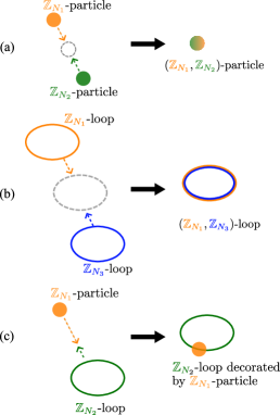
Figure 3: (a) Fusion of a $\mathbb{Z}_{N_{1}}$-particle and a $\mathbb{Z}_{N_{2}}$-particle. In continuous field theory, fusion of two particle excitations means that they moves towards each other until they meet at the same spatial location. This can be realized by making the world-lines of these two particles identical. The output of this fusion is a $\left(\mathbb{Z}_{N_{1}},\mathbb{Z}_{N_{2}}\right)$-particle which carries one unit of $\mathbb{Z}_{N_{1}}$ and $\mathbb{Z}_{N_{2}}$ gauge charge simultaneously. The $\mathbb{Z}_{N_{1}}$ and $\mathbb{Z}_{N_{2}}$ gauge charges in the output particle are represented by a mixed color of orange ($\mathbb{Z}_{N_{1}}$) and green ($\mathbb{Z}_{N_{2}}$). (b) Fusion of a $\mathbb{Z}_{N_{1}}$-loop and a $\mathbb{Z}_{N_{3}}$-loop. Similarly, fusion of two loops requires that they overlap at the same location. For this purpose, one can set their world-sheets identical in field theory. The result of this fusion is a loop carrying one unit of $\mathbb{Z}_{N_{1}}$ and $\mathbb{Z}_{N_{3}}$ flux respectively. These two fluxes are illustrated by two colors (orange and blue) circling along the loop. Notice that the boundary of two colors does not indicate a separation of two different fluxes. According to Table 2, a $\left(\mathbb{Z}_{N_{1}},\mathbb{Z}_{N_{3}}\right)$-loop is equivalent to a $\mathbb{Z}_{N_{1}}$-loop. (c) Fusion of a $\mathbb{Z}_{N_{1}}$-particle and a $\mathbb{Z}_{N_{2}}$-loop. The outcome is a decorated loop: a $\mathbb{Z}_{N_{2}}$-loop decorated by a $\mathbb{Z}_{N_{1}}$-particle. In fact, this is the definition of fusion of particle and loop. In continuous field theory, this fusion is realized by making the world-line of particle live on the world-sheet of loop.

III.1 Examples of fusion rule calculation

Now we explain how to exploit Eq. (31) to obtain fusion rules of topological excitations by several examples. These examples of fusion are illustrated in Fig. 4 in which two are Abelian fusion and the others are non-Abelian. The technical details can be found in Appendix C. The notations of operators ($\mathsf{P}_{n_{1}n_{2}n_{3}}$, $\mathsf{L}_{n_{1}n_{2}n_{3}}$, and $\mathsf{L}_{n_{1}n_{2}n_{3}}^{c_{1}c_{2}c_{3}}$) are also used to refer corresponding topological excitations in the context without causing ambiguity, e.g., $\mathsf{P}_{100}$ not only represents the operator of $\mathbb{Z}_{N_{1}}$-particle but also denotes the $\mathbb{Z}_{N_{1}}$-particle excitation itself. When we mention topological excitations in the fusion and loop shrinking operations (discussed in Sec. III.3), we use “$\otimes$” and “$\oplus$” between the notations for direct product and direct sum of fusion spaces. When Wilson operators in path integrals are consider, their multiplication and addition are indicated by “$\times$” and “$+$”.

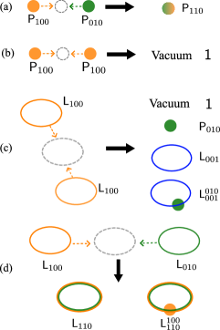
Figure 4: Illustrations of four fusion processes that are discussed in Sec. III.1 and detailed in Appendix C. (a) Fusion: $\mathsf{P}_{100}\otimes\mathsf{P}_{010}=\mathsf{P}_{110}$. This is an Abelian fusion: fusing a $\mathbb{Z}_{N_{1}}$-particle and a $\mathbb{Z}_{N_{2}}$-particle results a $\left(\mathbb{Z}_{N_{1}},\mathbb{Z}_{N_{2}}\right)$-particle. (b) Fusion: $\mathsf{P}_{100}\otimes\mathsf{P}_{100}=\mathsf{1}$. This is also an Abelian fusion. This fusion rule indicates that in BR topological order with $G=\left(\mathbb{Z}_{2}\right)^{3}$ the anti-particle of $\mathbb{Z}_{N_{1}}$-particle is itself. This make sense since the $\mathbb{Z}_{N_{1}}$ gauge subgroup is a $\mathbb{Z}_{2}$ group. (c) Non-Abelian fusion: $\mathsf{L}_{100}\otimes\mathsf{L}_{100}=\mathsf{1}\oplus\mathsf{P}_{010}\oplus\mathsf{L}_{001}\oplus\mathsf{L}_{001}^{010}$. Fusion of two $\mathbb{Z}_{N_{1}}$-loops produces not a determined outcome, but a superposition of a vacuum $\mathsf{1}$, a particle $\mathsf{P}_{010}$, a pure loop $\mathsf{L}_{001}$, and a decorated loop $\mathsf{L}_{001}^{010}$. (d) Non-Abelian fusion: $\mathsf{L}_{100}\otimes\mathsf{L}_{010}=\mathsf{L}_{110}\oplus\mathsf{L}_{110}^{100}$. The outcome of fusing a $\mathbb{Z}_{N_{1}}$-loop and a $\mathbb{Z}_{N_{2}}$-loop is a superposition of a pure loop ($\mathsf{L}_{110}$) and a decorated loop ($\mathsf{L}_{110}^{100}$). Notice that $\mathsf{L}_{110}$ and $\mathsf{L}_{110}^{100}$ are nonequivalent according to Table. 2 and Table. 3.

III.1.1 $\mathbb{Z}_{N_{1}}$-particle and $\mathbb{Z}_{N_{2}}$-particle

The 1 example is the fusion of a $\mathbb{Z}_{N_{1}}$-particle and a $\mathbb{Z}_{N_{2}}$-particle. Using Eq. 31, we can write down

$$\left\langle\mathsf{P}_{100}\otimes\mathsf{P}_{010}\right\rangle$$

$$= \frac{1}{\mathcal{Z}}\int\mathcal{D}\left[A^{i}\right]\mathcal{D}\left[B^{i}\right]\exp\left({\rm i}S\right)\mathsf{P}_{100}\times\mathsf{P}_{010}$$

$$= \frac{1}{\mathcal{Z}}\int\mathcal{D}\left[A^{i}\right]\mathcal{D}\left[B^{i}\right]\exp\left({\rm i}S\right)\exp\left({\rm i}\int_{\gamma}A^{1}+A^{2}\right)$$

$$= \frac{1}{\mathcal{Z}}\int\mathcal{D}\left[A^{i}\right]\mathcal{D}\left[B^{i}\right]\exp\left({\rm i}S\right)\mathsf{P}_{110}$$

$$= \left\langle\mathsf{P}_{110}\right\rangle$$ (32)

and find that

$$\mathsf{P}_{100}\otimes\mathsf{P}_{010}=\mathsf{P}_{110}.$$ (33)

This result indicates that by fusing two particles carrying $\mathbb{Z}_{N_{1}}$ and $\mathbb{Z}_{N_{2}}$ gauge charges respectively we obtain a single particle that carries both $\mathbb{Z}_{N_{1}}$ and $\mathbb{Z}_{N_{2}}$ gauge charges.

III.1.2 Two $\mathbb{Z}_{N_{1}}$-particles

The 2 example is the fusion of two $\mathbb{Z}_{N_{1}}$-particles:

$$\left\langle\mathsf{P}_{100}\otimes\mathsf{P}_{100}\right\rangle= \frac{1}{\mathcal{Z}}\int\mathcal{D}\left[A^{i}\right]\mathcal{D}\left[B^{i}\right]\exp\left({\rm i}S\right)\exp\left({\rm i}2\int_{\gamma}A^{1}\right).$$ (34)

Integrating out $B^{1}$, $B^{2}$, and $A^{3}$ and we obtain constraints for $A^{1}$, $A^{2}$, and $B^{3}$ respectively:

$$\oint A^{1}=\frac{2\pi m_{1}}{N_{1}},$$ (35)

$$\oint A^{2}=\frac{2\pi m_{2}}{N_{2}},$$ (36)

$$\oint B^{3}=\frac{2\pi m_{3}}{N_{3}},$$ (37)

where $m_{1,2,3}\in\mathbb{Z}$. Notice that gauge group is $G=\prod_{i=1}^{3}\mathbb{Z}_{N_{i}}=\left(\mathbb{Z}_{2}\right)^{3}$, we have

$$\left\langle\mathsf{P}_{100}\otimes\mathsf{P}_{100}\right\rangle=1=\left\langle\mathsf{1}\right\rangle,$$ (38)

i.e.,

$$\mathsf{P}_{100}\otimes\mathsf{P}_{100}=\mathsf{1}.$$ (39)

This result tells us that $\mathsf{P}_{100}$ is the anti-particle of itself , which is reasonable since $\mathsf{P}_{100}$ carries one unit of $\mathbb{Z}_{N_{1}}=\mathbb{Z}_{2}$ gauge charge.

III.1.3 Two $\mathbb{Z}_{N_{1}}$-loops

In the 3 example, we consider the fusion of two $\mathbb{Z}_{N_{1}}$-loops. We start with

$$\left\langle\mathsf{L}_{100}\otimes\mathsf{L}_{100}\right\rangle= \frac{1}{\mathcal{Z}}\int\mathcal{D}\left[A^{i}\right]\mathcal{D}\left[B^{i}\right]\exp\left({\rm i}S\right)\times\mathsf{L}_{100}\times\mathsf{L}_{100}.$$ (40)

Using Table. 2, we plug in the expression of $\mathsf{L}_{100}$ and obtain (details are collected in Appendix C):

$$\left\langle\mathsf{L}_{100}\otimes\mathsf{L}_{100}\right\rangle$$

$$= 1+\exp\left(\frac{{\rm i}2\pi m_{2}}{2}\right)+\exp\left(\frac{{\rm i}2\pi m_{3}}{2}\right)+\exp\left[\frac{{\rm i}2\pi\left(m_{2}+m_{3}\right)}{2}\right].$$ (41)

We can immediately find that

$$\left\langle\mathsf{L}_{100}\otimes\mathsf{L}_{100}\right\rangle$$

$$= \frac{1}{\mathcal{Z}}\int\mathcal{D}\left[A^{i}\right]\mathcal{D}\left[B^{i}\right]\exp\left({\rm i}S\right)\times\left(\mathsf{1}+\mathsf{P}_{010}+\mathsf{L}_{001}+\mathsf{L}_{001}^{010}\right)$$ (42)

thus we can conclude with

$$\mathsf{L}_{100}\otimes\mathsf{L}_{100}=\mathsf{1}\oplus\mathsf{P}_{010}\oplus\mathsf{L}_{001}\oplus\mathsf{L}_{001}^{010}.$$ (43)

This is a non-Abelian fusion rule which tells us that if we fuse two $\mathbb{Z}_{N_{1}}$-loops we would obtain the superposition of a vacuum, a $\mathbb{Z}_{N_{2}}$-particle, a $\mathbb{Z}_{N_{3}}$-loop, and a $\mathbb{Z}_{N_{3}}$-loop decorated by a $\mathbb{Z}_{N_{2}}$-particle.

III.1.4 $\mathbb{Z}_{N_{1}}$-loop and $\mathbb{Z}_{N_{2}}$-loop

In the 4 example, we continue to consider $\mathsf{L}_{100}\otimes\mathsf{L}_{010}$:

$$\left\langle\mathsf{L}_{100}\otimes\mathsf{L}_{010}\right\rangle$$

$$= \frac{1}{\mathcal{Z}}\int\mathcal{D}\left[A^{i}\right]\mathcal{D}\left[B^{i}\right]\exp\left({\rm i}S\right)\times\mathsf{L}_{100}\times\mathsf{L}_{010}.$$ (44)

For simplicity, we denote $\mathsf{L}_{100}\times\mathsf{L}_{010}$ as

$$\mathsf{L}_{100}\times\mathsf{L}_{010}= 4\exp\left({\rm i}f_{1}+{\rm i}f_{2}\right)\delta\left(\int_{\gamma}A^{2}\right)\delta\left(\int_{\sigma}B^{3}\right)$$

$$\times\delta\left(\int_{\gamma}A^{1}\right)\delta\left(\int_{\sigma}B^{3}\right)$$ (45)

where $f_{1}=\int_{\sigma}B^{1}+\frac{1}{2}\frac{2\pi q}{N_{1}}\left(d^{-1}A^{2}B^{3}+d^{-1}B^{3}A^{2}\right)$ and $f_{2}=\int_{\sigma}B^{2}-\frac{1}{2}\frac{2\pi q}{N_{2}}\left(d^{-1}B^{3}A^{1}+d^{-1}A^{1}B^{3}\right)$. For the complete expression of $\mathsf{L}_{100}$ and $\mathsf{L}_{010}$, one can refer to Table 2. Since the Kronecker delta functions can be re-written as

$$\delta\left(\int_{\sigma}B^{3}\right)\delta\left(\int_{\sigma}B^{3}\right)= \delta\left(\int_{\sigma}B^{3}\right),$$ (46)

$$\delta\left(\int_{\gamma}A^{2}\right)\delta\left(\int_{\gamma}A^{1}\right)= \delta\left(\int_{\gamma}A^{2}-A^{1}\right)\delta\left(\int_{\gamma}A^{1}\right),$$ (47)

we can write $\mathsf{L}_{100}\times\mathsf{L}_{010}$ as

$$\mathsf{L}_{100}\times\mathsf{L}_{010}= 4\exp\left({\rm i}f_{1}+{\rm i}f_{2}\right)\delta\left(\int_{\gamma}A^{1}\right)$$

$$\times\delta\left(\int_{\gamma}A^{2}-A^{1}\right)\delta\left(\int_{\sigma}B^{3}\right).$$ (48)

The Kronecker delta function $\delta\left(\int_{\gamma}A^{1}\right)$ can be expressed as $\delta\left(\int_{\gamma}A^{1}\right)=\frac{1}{2}\left[1+\exp\left({\rm i}\int_{\gamma}A^{1}\right)\right]$ in path integral. Therefore, in the sense of expectation value,

$$\mathsf{L}_{100}\times\mathsf{L}_{010}= 2\exp\left({\rm i}f_{1}+{\rm i}f_{2}+{\rm i}\int_{\gamma}A^{1}\right)$$

$$\times\delta\left(\int_{\gamma}A^{2}-A^{1}\right)\delta\left(\int_{\sigma}B^{3}\right).$$ (49)

By checking the all $19$ operators, we find (here $\mathsf{L}$ denotes operators of loops)

$$\left\langle\mathsf{L}_{100}\times\mathsf{L}_{010}\right\rangle= \left\langle\mathsf{L}_{110}+\mathsf{L}_{110}^{100}\right\rangle$$ (50)

which indicates the following fusion rule of topological excitations (here $\mathsf{L}$ denotes loop excitations):

$$\mathsf{L}_{100}\otimes\mathsf{L}_{010}=\mathsf{L}_{110}\oplus\mathsf{L}_{110}^{100}.$$ (51)

This is another non-Abelian fusion rule. The output of fusion of a $\mathbb{Z}_{N_{1}}$-loop and a $\mathbb{Z}_{N_{2}}$-loop is the superposition of a pure $\left(\mathbb{Z}_{N_{1}},\mathbb{Z}_{N_{2}}\right)$-loop, $\mathsf{L}_{110}$ and a $\left(\mathbb{Z}_{N_{1}},\mathbb{Z}_{N_{2}}\right)$-loop decorated by a $\mathbb{Z}_{N_{1}}$-particle, $\mathsf{L}_{110}^{100}$. One should notice the following equivalence relation as indicated in Table. 3: $\mathsf{L}_{110}=\mathsf{L}_{110}^{110}$ and $\mathsf{L}_{110}^{100}=\mathsf{L}_{110}^{010}$. The above results are obtained through a calculation of path integral though the formulas are written in a simplified manner. The detailed derivation can be found in Appendix C.

III.2 Fusion table for BR topological order with $G=\left(\mathbb{Z}_{2}\right)^{3}$

The above examples show how to calculate fusion rules from path integral. By exhausting all combinations of two excitations, we obtain the complete fusion rules and quantum dimension $d$ of excitations for Borromean rings topological order with $G=\left(\mathbb{Z}_{2}\right)^{3}$ as shown in Table 4 and Table 5. The fusion rules satisfy the properties of commutativity and associativity, i.e., $\mathsf{a}\otimes\mathsf{b}=\mathsf{b}\otimes\mathsf{a}$ and $\left(\mathsf{a}\otimes\mathsf{b}\right)\otimes\mathsf{c}=\mathsf{a}\otimes\left(\mathsf{b}\otimes\mathsf{c}\right)$, which is automatically guaranteed by the path integral calculation of Abelian gauge fields.

In the BR topological order with $G=\left(\mathbb{Z}_{2}\right)^{3}$, the excitations can be divided as follows: vacuum, $\mathsf{1}$; $4$ nonequivalent particles, $\mathsf{P}_{100}$, $\mathsf{P}_{010}$, $\mathsf{P}_{110}$, and $\mathsf{P_{001}}$; $4$ nonequivalent pure loops, $\mathsf{L}_{001}$, $\mathsf{L}_{100}$, $\mathsf{L}_{010}$, and $\mathsf{L}_{110}$; $10$ nonequivalent loops decorated with particle, $\mathsf{L}_{001}^{100}$, $\mathsf{L}_{001}^{010}$, $\mathsf{L}_{001}^{110}$, $\mathsf{L}_{100}^{100}$, $\mathsf{L}_{010}^{010}$, $\mathsf{L}_{001}^{001}$, $\mathsf{L}_{110}^{100}$, $\mathsf{L}_{100}^{001}$, $\mathsf{L}_{010}^{001}$, and $\mathsf{L}_{110}^{001}$. All these excitations, no matter particles or loops, can be thought as combinations of gauge charges and gauge fluxes. Since the gauge group is $G=\left(\mathbb{Z}_{2}\right)^{3}$, one may find there are $\left(2^{3}\right)^{2}=64$ different combinations that exceeds the number of excitations listed in Table 4. In fact, among all $64$ combinations of gauge charges and fluxes, some of them behave without any difference thus collected to the same equivalence class, as shown in Sec. II.2 and Table 3.

In the following lines, we make some explanation about the Table 4 of fusion rules. First, there are $8$ Abelian excitations ($\mathsf{1}$, $\mathsf{P}_{100}$, $\mathsf{P}_{010}$, $\mathsf{L}_{001}$, $\mathsf{P}_{110}$, $\mathsf{L}_{001}^{100}$, $\mathsf{L}_{001}^{010}$, and $\mathsf{L}_{001}^{110}$; labeled by number $1$ to $8$ in Table 4) whose fusion rules with any other excitations are always Abelian, i.e., single fusion channel. All other excitations are called non-Abelian excitations. This fusion table is obtained in the case of $G=\left(\mathbb{Z}_{2}\right)^{3}$ and we may expect that the fusion of an excitation and itself would produce a vacuum due to the $\mathbb{Z}_{2}$ cyclic nature. Nevertheless, for $\mathsf{L}_{100}^{001}$, a loop carrying $\mathbb{Z}_{N_{1}}$ flux and decorated by a $\mathbb{Z}_{N_{3}}$-particle, the fusion of two $\mathsf{L}_{100}^{001}$ produces two copies of the direct sum of all $8$ Abelian excitations that is denoted as $\mathbf{Ab}$ (see Table 4). This means that $\mathsf{L}_{100}^{001}\otimes\mathsf{L}_{100}^{001}$ generates a direct sum of two vacuums. Meanwhile, $\mathsf{L}_{010}^{001}$ and $\mathsf{L}_{110}^{001}$ also have this property. Field-theoretical calculation for this result can be found in Appendix C.5. For other excitations, the fusion of its two copies just produce a single vacuum.

From this fusion table, we can obtain all fusion coefficients $N_{k}^{ij}$’s and matrices $N_{i}$ whose element is $\left(N_{i}\right)_{kj}=N_{k}^{ij}$, where $i,j,k$ are integers ranging from $1$ to $19$ to label the topological excitations. The largest eigenvalue of $N_{i}$ is the quantum dimension of corresponding excitations, as shown in Table 5. We notice that the quantum dimension of topological excitation is exactly the coefficient in the front of corresponding gauge-invariant operator. This fact may imply a connection between the Wilson operator and the fusion space of a topological excitation. Finally, we note that, non-Abelian fusion rules are also found in $\left(2+1\right)$D DW gauge theory with Abelian gauge group (Propitius, 1995; He et al., 2017), where it is found that for a gauge group $G=\left(\mathbb{Z}_{2}\right)^{3}$, the fusion rules for particles can be captured by the so-called twisted quantum double model $D^{\omega_{3}}(G)$. Yet the present situation in $\left(3+1\right)$D is different: we still consider a $G=\left(\mathbb{Z}_{2}\right)^{3}$ gauge group as a simple illustration, the algebra of fusion rules is apparently different from that of $D^{\omega_{3}}(G)$.

Table 4: Complete fusion rules of excitations for BR topological order with $G=\left(\mathbb{Z}_{2}\right)^{3}$. Numbers $1$ to $19$ are used to label the nineteen different excitations. For excitations labeled by $1$ to $8$, their fusion rules with any other excitations are always Abelian so we call them Abelian excitations. The remaining excitations are dubbed non-Abelian excitations since among all fusion rules only the ones involving them are non-Abelian. $\mathbf{Ab}$ denotes the direct sum of all the Abelian excitations: $\mathbf{Ab}\equiv\mathsf{1}\oplus\mathsf{P}_{100}\oplus\mathsf{P}_{010}\oplus\mathsf{L}_{001}\oplus\mathsf{P}_{110}\oplus\mathsf{L}_{001}^{100}\oplus\mathsf{L}_{001}^{010}\oplus\mathsf{L}_{001}^{110}$. All these fusion rules are obtained using field-theoretical approach. Some of them are explained as examples in Sec. III.1 and Appendix C.

		Abelian excitations								non-Abelian excitations
	$\otimes$	$\mathsf{1}$	$\mathsf{P}_{100}$	$\mathsf{P}_{010}$	$\mathsf{L}_{001}$	$\mathsf{P}_{110}$	$\mathsf{L}_{001}^{100}$	$\mathsf{L}_{001}^{010}$	$\mathsf{L}_{001}^{110}$	$\mathsf{L}_{100}$	$\mathsf{L}_{100}^{100}$	$\mathsf{L}_{010}$	$\mathsf{L}_{010}^{010}$	$\mathsf{P}_{001}$	$\mathsf{L}_{001}^{001}$	$\mathsf{L}_{110}$	$\mathsf{L}_{110}^{100}$	$\mathsf{L}_{100}^{001}$	$\mathsf{L}_{010}^{001}$	$\mathsf{L}_{110}^{001}$
1	$\mathsf{1}$	$\mathsf{1}$	$\mathsf{P}_{100}$	$\mathsf{P}_{010}$	$\mathsf{L}_{001}$	$\mathsf{P}_{110}$	$\mathsf{L}_{001}^{100}$	$\mathsf{L}_{001}^{010}$	$\mathsf{L}_{001}^{110}$	$\mathsf{L}_{100}$	$\mathsf{L}_{100}^{100}$	$\mathsf{L}_{010}$	$\mathsf{L}_{010}^{010}$	$\mathsf{P}_{001}$	$\mathsf{L}_{001}^{001}$	$\mathsf{L}_{110}$	$\mathsf{L}_{110}^{100}$	$\mathsf{L}_{100}^{001}$	$\mathsf{L}_{010}^{001}$	$\mathsf{L}_{110}^{001}$
2	$\mathsf{P}_{100}$	$\mathsf{P}_{100}$	$\mathsf{1}$	$\mathsf{P}_{110}$	$\mathsf{L}_{001}^{100}$	$\mathsf{P}_{010}$	$\mathsf{L}_{001}$	$\mathsf{L}_{001}^{110}$	$\mathsf{L}_{001}^{010}$	$\mathsf{L}_{100}^{100}$	$\mathsf{L}_{100}$	$\mathsf{L}_{010}$	$\mathsf{L}_{010}^{010}$	$\mathsf{P}_{001}$	$\mathsf{L}_{001}^{001}$	$\mathsf{L}_{110}^{100}$	$\mathsf{L}_{110}$	$\mathsf{L}_{100}^{001}$	$\mathsf{L}_{010}^{001}$	$\mathsf{L}_{110}^{001}$
3	$\mathsf{P}_{010}$	$\mathsf{P}_{010}$	$\mathsf{P}_{110}$	$\mathsf{1}$	$\mathsf{L}_{001}^{010}$	$\mathsf{P}_{100}$	$\mathsf{L}_{001}^{110}$	$\mathsf{L}_{001}$	$\mathsf{L}_{001}^{100}$	$\mathsf{L}_{100}$	$\mathsf{L}_{100}^{100}$	$\mathsf{L}_{010}^{010}$	$\mathsf{L}_{010}$	$\mathsf{P}_{001}$	$\mathsf{L}_{001}^{001}$	$\mathsf{L}_{110}^{100}$	$\mathsf{L}_{110}$	$\mathsf{L}_{100}^{001}$	$\mathsf{L}_{010}^{001}$	$\mathsf{L}_{110}^{001}$
4	$\mathsf{L}_{001}$	$\mathsf{L}_{001}$	$\mathsf{L}_{001}^{100}$	$\mathsf{L}_{001}^{010}$	$\mathsf{1}$	$\mathsf{L}_{001}^{110}$	$\mathsf{P}_{100}$	$\mathsf{P}_{010}$	$\mathsf{P}_{110}$	$\mathsf{L}_{100}$	$\mathsf{L}_{100}^{100}$	$\mathsf{L}_{010}$	$\mathsf{L}_{010}^{010}$	$\mathsf{L}_{001}^{001}$	$\mathsf{P}_{001}$	$\mathsf{L}_{110}$	$\mathsf{L}_{110}^{100}$	$\mathsf{L}_{100}^{001}$	$\mathsf{L}_{010}^{001}$	$\mathsf{L}_{110}^{001}$
5	$\mathsf{P}_{110}$	$\mathsf{P}_{110}$	$\mathsf{P}_{010}$	$\mathsf{P}_{100}$	$\mathsf{L}_{001}^{110}$	$\mathsf{1}$	$\mathsf{L}_{001}^{010}$	$\mathsf{L}_{001}^{100}$	$\mathsf{L}_{001}$	$\mathsf{L}_{100}^{100}$	$\mathsf{L}_{100}$	$\mathsf{L}_{010}^{010}$	$\mathsf{L}_{010}$	$\mathsf{P}_{001}$	$\mathsf{L}_{001}^{001}$	$\mathsf{L}_{110}$	$\mathsf{L}_{110}^{100}$	$\mathsf{L}_{100}^{001}$	$\mathsf{L}_{010}^{001}$	$\mathsf{L}_{110}^{001}$
6	$\mathsf{L}_{001}^{100}$	$\mathsf{L}_{001}^{100}$	$\mathsf{L}_{001}$	$\mathsf{L}_{001}^{110}$	$\mathsf{P}_{100}$	$\mathsf{L}_{001}^{010}$	$\mathsf{1}$	$\mathsf{P}_{110}$	$\mathsf{P}_{010}$	$\mathsf{L}_{100}^{100}$	$\mathsf{L}_{100}$	$\mathsf{L}_{010}$	$\mathsf{L}_{010}^{010}$	$\mathsf{L}_{001}^{001}$	$\mathsf{P}_{001}$	$\mathsf{L}_{110}^{100}$	$\mathsf{L}_{110}$	$\mathsf{L}_{100}^{001}$	$\mathsf{L}_{010}^{001}$	$\mathsf{L}_{110}^{001}$
7	$\mathsf{L}_{001}^{010}$	$\mathsf{L}_{001}^{010}$	$\mathsf{L}_{001}^{110}$	$\mathsf{L}_{001}$	$\mathsf{P}_{010}$	$\mathsf{L}_{001}^{100}$	$\mathsf{P}_{110}$	$\mathsf{1}$	$\mathsf{P}_{100}$	$\mathsf{L}_{100}$	$\mathsf{L}_{100}^{100}$	$\mathsf{L}_{010}^{010}$	$\mathsf{L}_{010}$	$\mathsf{L}_{001}^{001}$	$\mathsf{P}_{001}$	$\mathsf{L}_{110}^{100}$	$\mathsf{L}_{110}$	$\mathsf{L}_{100}^{001}$	$\mathsf{L}_{010}^{001}$	$\mathsf{L}_{110}^{001}$
8	$\mathsf{L}_{001}^{110}$	$\mathsf{L}_{001}^{110}$	$\mathsf{L}_{001}^{010}$	$\mathsf{L}_{001}^{100}$	$\mathsf{P}_{110}$	$\mathsf{L}_{001}$	$\mathsf{P}_{010}$	$\mathsf{P}_{100}$	$\mathsf{1}$	$\mathsf{L}_{100}^{100}$	$\mathsf{L}_{100}$	$\mathsf{L}_{010}^{010}$	$\mathsf{L}_{010}$	$\mathsf{L}_{001}^{001}$	$\mathsf{P}_{001}$	$\mathsf{L}_{110}$	$\mathsf{L}_{110}^{100}$	$\mathsf{L}_{100}^{001}$	$\mathsf{L}_{010}^{001}$	$\mathsf{L}_{110}^{001}$
9	$\mathsf{L}_{100}$	$\mathsf{L}_{100}$	$\mathsf{L}_{100}^{100}$	$\mathsf{L}_{100}$	$\mathsf{L}_{100}$	$\mathsf{L}_{100}^{100}$	$\mathsf{L}_{100}^{100}$	$\mathsf{L}_{100}$	$\mathsf{L}_{100}^{100}$	$\begin{aligned} &\mathsf{1}\\ \oplus&\mathsf{P}_{010}\\ \oplus&\mathsf{L}_{001}\\ \oplus&\mathsf{L}_{001}^{010}\end{aligned}$	$\begin{aligned} &\mathsf{P}_{100}\\ \oplus&\mathsf{P}_{110}\\ \oplus&\mathsf{L}_{001}^{100}\\ \oplus&\mathsf{L}_{001}^{110}\end{aligned}$	$\begin{aligned} &\mathsf{L}_{110}\\ \oplus&\mathsf{L}_{110}^{100}\end{aligned}$	$\begin{aligned} &\mathsf{L}_{110}\\ \oplus&\mathsf{L}_{110}^{100}\end{aligned}$	$\mathsf{L}_{100}^{001}$	$\mathsf{L}_{100}^{001}$	$\begin{aligned} &\mathsf{L}_{010}\\ \oplus&\mathsf{L}_{010}^{010}\end{aligned}$	$\begin{aligned} &\mathsf{L}_{010}\\ \oplus&\mathsf{L}_{010}^{010}\end{aligned}$	$\begin{aligned} &2\cdot\mathsf{P}_{001}\\ \oplus&2\cdot\mathsf{L}_{001}^{001}\end{aligned}$	$2\cdot\mathsf{L}_{110}^{001}$	$2\cdot\mathsf{L}_{010}^{001}$
10	$\mathsf{L}_{100}^{100}$	$\mathsf{L}_{100}^{100}$	$\mathsf{L}_{100}$	$\mathsf{L}_{100}^{100}$	$\mathsf{L}_{100}^{100}$	$\mathsf{L}_{100}$	$\mathsf{L}_{100}$	$\mathsf{L}_{100}^{100}$	$\mathsf{L}_{100}$	$\begin{aligned} &\mathsf{P}_{100}\\ \oplus&\mathsf{P}_{110}\\ \oplus&\mathsf{L}_{001}^{100}\\ \oplus&\mathsf{L}_{001}^{110}\end{aligned}$	$\begin{aligned} &\mathsf{1}\\ \oplus&\mathsf{P}_{010}\\ \oplus&\mathsf{L}_{001}\\ \oplus&\mathsf{L}_{001}^{010}\end{aligned}$	$\begin{aligned} &\mathsf{L}_{110}\\ \oplus&\mathsf{L}_{110}^{100}\end{aligned}$	$\begin{aligned} &\mathsf{L}_{110}\\ \oplus&\mathsf{L}_{110}^{100}\end{aligned}$	$\mathsf{L}_{100}^{001}$	$\mathsf{L}_{100}^{001}$	$\begin{aligned} &\mathsf{L}_{010}\\ \oplus&\mathsf{L}_{010}^{010}\end{aligned}$	$\begin{aligned} &\mathsf{L}_{010}\\ \oplus&\mathsf{L}_{010}^{010}\end{aligned}$	$\begin{aligned} &2\cdot\mathsf{P}_{001}\\ \oplus&2\cdot\mathsf{L}_{001}^{001}\end{aligned}$	$2\cdot\mathsf{L}_{110}^{001}$	$2\cdot\mathsf{L}_{010}^{001}$
11	$\mathsf{L}_{010}$	$\mathsf{L}_{010}$	$\mathsf{L}_{010}$	$\mathsf{L}_{010}^{010}$	$\mathsf{L}_{010}$	$\mathsf{L}_{010}^{010}$	$\mathsf{L}_{010}$	$\mathsf{L}_{010}^{010}$	$\mathsf{L}_{010}^{010}$	$\begin{aligned} &\mathsf{L}_{110}\\ \oplus&\mathsf{L}_{110}^{100}\end{aligned}$	$\begin{aligned} &\mathsf{L}_{110}\\ \oplus&\mathsf{L}_{110}^{100}\end{aligned}$	$\begin{aligned} &\mathsf{1}\\ \oplus&\mathsf{L}_{001}\\ \oplus&\mathsf{P}_{100}\\ \oplus&\mathsf{L}_{001}^{100}\end{aligned}$	$\begin{aligned} &\mathsf{P}_{010}\\ \oplus&\mathsf{L}_{001}^{010}\\ \oplus&\mathsf{P}_{110}\\ \oplus&\mathsf{L}_{001}^{110}\end{aligned}$	$\mathsf{L}_{010}^{001}$	$\mathsf{L}_{010}^{001}$	$\begin{aligned} &\mathsf{L}_{100}\\ \oplus&\mathsf{L}_{100}^{100}\end{aligned}$	$\begin{aligned} &\mathsf{L}_{100}\\ \oplus&\mathsf{L}_{100}^{100}\end{aligned}$	$2\cdot\mathsf{L}_{110}^{001}$	$\begin{aligned} &2\cdot\mathsf{P}_{001}\\ \oplus&2\cdot\mathsf{L}_{001}^{001}\end{aligned}$	$2\cdot\mathsf{L}_{100}^{001}$
12	$\mathsf{L}_{010}^{010}$	$\mathsf{L}_{010}^{010}$	$\mathsf{L}_{010}^{010}$	$\mathsf{L}_{010}$	$\mathsf{L}_{010}^{010}$	$\mathsf{L}_{010}$	$\mathsf{L}_{010}^{010}$	$\mathsf{L}_{010}$	$\mathsf{L}_{010}$	$\begin{aligned} &\mathsf{L}_{110}\\ \oplus&\mathsf{L}_{110}^{100}\end{aligned}$	$\begin{aligned} &\mathsf{L}_{110}\\ \oplus&\mathsf{L}_{110}^{100}\end{aligned}$	$\begin{aligned} &\mathsf{P}_{010}\\ \oplus&\mathsf{L}_{001}^{010}\\ \oplus&\mathsf{P}_{110}\\ \oplus&\mathsf{L}_{001}^{110}\end{aligned}$	$\begin{aligned} &\mathsf{1}\\ \oplus&\mathsf{L}_{001}\\ \oplus&\mathsf{P}_{100}\\ \oplus&\mathsf{L}_{001}^{100}\end{aligned}$	$\mathsf{L}_{010}^{001}$	$\mathsf{L}_{010}^{001}$	$\begin{aligned} &\mathsf{L}_{100}\\ \oplus&\mathsf{L}_{100}^{100}\end{aligned}$	$\begin{aligned} &\mathsf{L}_{100}\\ \oplus&\mathsf{L}_{100}^{100}\end{aligned}$	$2\cdot\mathsf{L}_{110}^{001}$	$\begin{aligned} &2\cdot\mathsf{P}_{001}\\ \oplus&2\cdot\mathsf{L}_{001}^{001}\end{aligned}$	$2\cdot\mathsf{L}_{100}^{001}$
13	$\mathsf{P}_{001}$	$\mathsf{P}_{001}$	$\mathsf{P}_{001}$	$\mathsf{P}_{001}$	$\mathsf{L}_{001}^{001}$	$\mathsf{P}_{001}$	$\mathsf{L}_{001}^{001}$	$\mathsf{L}_{001}^{001}$	$\mathsf{L}_{001}^{001}$	$\mathsf{L}_{100}^{001}$	$\mathsf{L}_{100}^{001}$	$\mathsf{L}_{010}^{001}$	$\mathsf{L}_{010}^{001}$	$\begin{aligned} &\mathsf{1}\\ \oplus&\mathsf{P}_{100}\\ \oplus&\mathsf{P}_{010}\\ \oplus&\mathsf{P}_{110}\end{aligned}$	$\begin{aligned} &\mathsf{L}_{001}\\ \oplus&\mathsf{L}_{001}^{100}\\ \oplus&\mathsf{L}_{001}^{010}\\ \oplus&\mathsf{L}_{001}^{110}\end{aligned}$	$\mathsf{L}_{110}^{001}$	$\mathsf{L}_{110}^{001}$	$\begin{aligned} &2\cdot\mathsf{L}_{100}\\ \oplus&2\cdot\mathsf{L}_{100}^{100}\end{aligned}$	$\begin{aligned} &2\cdot\mathsf{L}_{010}\\ \oplus&2\cdot\mathsf{L}_{010}^{010}\end{aligned}$	$\begin{aligned} &2\cdot\mathsf{L}_{110}\\ \oplus&2\cdot\mathsf{L}_{110}^{100}\end{aligned}$
14	$\mathsf{L}_{001}^{001}$	$\mathsf{L}_{001}^{001}$	$\mathsf{L}_{001}^{001}$	$\mathsf{L}_{001}^{001}$	$\mathsf{P}_{001}$	$\mathsf{L}_{001}^{001}$	$\mathsf{P}_{001}$	$\mathsf{P}_{001}$	$\mathsf{P}_{001}$	$\mathsf{L}_{100}^{001}$	$\mathsf{L}_{100}^{001}$	$\mathsf{L}_{010}^{001}$	$\mathsf{L}_{010}^{001}$	$\begin{aligned} &\mathsf{L}_{001}\\ \oplus&\mathsf{L}_{001}^{100}\\ \oplus&\mathsf{L}_{001}^{010}\\ \oplus&\mathsf{L}_{001}^{110}\end{aligned}$	$\begin{aligned} &\mathsf{1}\\ \oplus&\mathsf{P}_{100}\\ \oplus&\mathsf{P}_{010}\\ \oplus&\mathsf{P}_{110}\end{aligned}$	$\mathsf{L}_{110}^{001}$	$\mathsf{L}_{110}^{001}$	$\begin{aligned} &2\cdot\mathsf{L}_{100}\\ \oplus&2\cdot\mathsf{L}_{100}^{100}\end{aligned}$	$\begin{aligned} &2\cdot\mathsf{L}_{010}\\ \oplus&2\cdot\mathsf{L}_{010}^{010}\end{aligned}$	$\begin{aligned} &2\cdot\mathsf{L}_{110}\\ \oplus&2\cdot\mathsf{L}_{110}^{100}\end{aligned}$
15	$\mathsf{L}_{110}$	$\mathsf{L}_{110}$	$\mathsf{L}_{110}^{100}$	$\mathsf{L}_{110}^{100}$	$\mathsf{L}_{110}$	$\mathsf{L}_{110}$	$\mathsf{L}_{110}^{100}$	$\mathsf{L}_{110}^{100}$	$\mathsf{L}_{110}$	$\begin{aligned} &\mathsf{L}_{010}\\ \oplus&\mathsf{L}_{010}^{010}\end{aligned}$	$\begin{aligned} &\mathsf{L}_{010}\\ \oplus&\mathsf{L}_{010}^{010}\end{aligned}$	$\begin{aligned} &\mathsf{L}_{100}\\ \oplus&\mathsf{L}_{100}^{100}\end{aligned}$	$\begin{aligned} &\mathsf{L}_{100}\\ \oplus&\mathsf{L}_{100}^{100}\end{aligned}$	$\mathsf{L}_{110}^{001}$	$\mathsf{L}_{110}^{001}$	$\begin{aligned} &\mathsf{1}\\ \oplus&\mathsf{P}_{110}\\ \oplus&\mathsf{L}_{001}\\ \oplus&\mathsf{L}_{001}^{110}\end{aligned}$	$\begin{aligned} &\mathsf{P}_{100}\\ \oplus&\mathsf{P}_{010}\\ \oplus&\mathsf{L}_{001}^{100}\\ \oplus&\mathsf{L}_{001}^{010}\end{aligned}$	$2\cdot\mathsf{L}_{010}^{001}$	$2\cdot\mathsf{L}_{100}^{001}$	$\begin{aligned} &2\cdot\mathsf{P}_{001}\\ \oplus&2\cdot\mathsf{L}_{001}^{001}\end{aligned}$
16	$\mathsf{L}_{110}^{100}$	$\mathsf{L}_{110}^{100}$	$\mathsf{L}_{110}$	$\mathsf{L}_{110}$	$\mathsf{L}_{110}^{100}$	$\mathsf{L}_{110}^{100}$	$\mathsf{L}_{110}$	$\mathsf{L}_{110}$	$\mathsf{L}_{110}^{100}$	$\begin{aligned} &\mathsf{L}_{010}\\ \oplus&\mathsf{L}_{010}^{010}\end{aligned}$	$\begin{aligned} &\mathsf{L}_{010}\\ \oplus&\mathsf{L}_{010}^{010}\end{aligned}$	$\begin{aligned} &\mathsf{L}_{100}\\ \oplus&\mathsf{L}_{100}^{100}\end{aligned}$	$\begin{aligned} &\mathsf{L}_{100}\\ \oplus&\mathsf{L}_{100}^{100}\end{aligned}$	$\mathsf{L}_{110}^{001}$	$\mathsf{L}_{110}^{001}$	$\begin{aligned} &\mathsf{P}_{100}\\ \oplus&\mathsf{P}_{010}\\ \oplus&\mathsf{L}_{001}^{100}\\ \oplus&\mathsf{L}_{001}^{010}\end{aligned}$	$\begin{aligned} &\mathsf{1}\\ \oplus&\mathsf{P}_{110}\\ \oplus&\mathsf{L}_{001}\\ \oplus&\mathsf{L}_{001}^{110}\end{aligned}$	$2\cdot\mathsf{L}_{010}^{001}$	$2\cdot\mathsf{L}_{100}^{001}$	$\begin{aligned} &2\cdot\mathsf{P}_{001}\\ \oplus&2\cdot\mathsf{L}_{001}^{001}\end{aligned}$
17	$\mathsf{L}_{100}^{001}$	$\mathsf{L}_{100}^{001}$	$\mathsf{L}_{100}^{001}$	$\mathsf{L}_{100}^{001}$	$\mathsf{L}_{100}^{001}$	$\mathsf{L}_{100}^{001}$	$\mathsf{L}_{100}^{001}$	$\mathsf{L}_{100}^{001}$	$\mathsf{L}_{100}^{001}$	$\begin{aligned} &2\cdot\mathsf{P}_{001}\\ \oplus&2\cdot\mathsf{L}_{001}^{001}\end{aligned}$	$\begin{aligned} &2\cdot\mathsf{P}_{001}\\ \oplus&2\cdot\mathsf{L}_{001}^{001}\end{aligned}$	$2\cdot\mathsf{L}_{110}^{001}$	$2\cdot\mathsf{L}_{110}^{001}$	$\begin{aligned} &2\cdot\mathsf{L}_{100}\\ \oplus&2\cdot\mathsf{L}_{100}^{100}\end{aligned}$	$\begin{aligned} &2\cdot\mathsf{L}_{100}\\ \oplus&2\cdot\mathsf{L}_{100}^{100}\end{aligned}$	$2\cdot\mathsf{L}_{010}^{001}$	$2\cdot\mathsf{L}_{010}^{001}$	$2\cdot\mathbf{Ab}$	$\begin{aligned} &4\cdot\mathsf{L}_{110}\\ \oplus&4\cdot\mathsf{L}_{110}^{100}\end{aligned}$	$\begin{aligned} &4\cdot\mathsf{L}_{010}\\ \oplus&4\cdot\mathsf{L}_{010}^{010}\end{aligned}$
18	$\mathsf{L}_{010}^{001}$	$\mathsf{L}_{010}^{001}$	$\mathsf{L}_{010}^{001}$	$\mathsf{L}_{010}^{001}$	$\mathsf{L}_{010}^{001}$	$\mathsf{L}_{010}^{001}$	$\mathsf{L}_{010}^{001}$	$\mathsf{L}_{010}^{001}$	$\mathsf{L}_{010}^{001}$	$2\cdot\mathsf{L}_{110}^{001}$	$2\cdot\mathsf{L}_{110}^{001}$	$\begin{aligned} &2\cdot\mathsf{P}_{001}\\ \oplus&2\cdot\mathsf{L}_{001}^{001}\end{aligned}$	$\begin{aligned} &2\cdot\mathsf{P}_{001}\\ \oplus&2\cdot\mathsf{L}_{001}^{001}\end{aligned}$	$\begin{aligned} &2\cdot\mathsf{L}_{010}\\ \oplus&2\cdot\mathsf{L}_{010}^{010}\end{aligned}$	$\begin{aligned} &2\cdot\mathsf{L}_{010}\\ \oplus&2\cdot\mathsf{L}_{010}^{010}\end{aligned}$	$2\cdot\mathsf{L}_{100}^{001}$	$2\cdot\mathsf{L}_{100}^{001}$	$\begin{aligned} &4\cdot\mathsf{L}_{110}\\ \oplus&4\cdot\mathsf{L}_{110}^{100}\end{aligned}$	$2\cdot\mathbf{Ab}$	$\begin{aligned} &4\cdot\mathsf{L}_{100}\\ \oplus&4\cdot\mathsf{L}_{100}^{100}\end{aligned}$
19	$\mathsf{L}_{110}^{001}$	$\mathsf{L}_{110}^{001}$	$\mathsf{L}_{110}^{001}$	$\mathsf{L}_{110}^{001}$	$\mathsf{L}_{110}^{001}$	$\mathsf{L}_{110}^{001}$	$\mathsf{L}_{110}^{001}$	$\mathsf{L}_{110}^{001}$	$\mathsf{L}_{110}^{001}$	$2\cdot\mathsf{L}_{010}^{001}$	$2\cdot\mathsf{L}_{010}^{001}$	$2\cdot\mathsf{L}_{100}^{001}$	$2\cdot\mathsf{L}_{100}^{001}$	$\begin{aligned} &2\cdot\mathsf{L}_{110}\\ \oplus&2\cdot\mathsf{L}_{110}^{100}\end{aligned}$	$\begin{aligned} &2\cdot\mathsf{L}_{110}\\ \oplus&2\cdot\mathsf{L}_{110}^{100}\end{aligned}$	$\begin{aligned} &2\cdot\mathsf{P}_{001}\\ \oplus&2\cdot\mathsf{L}_{001}^{001}\end{aligned}$	$\begin{aligned} &2\cdot\mathsf{P}_{001}\\ \oplus&2\cdot\mathsf{L}_{001}^{001}\end{aligned}$	$\begin{aligned} &4\cdot\mathsf{L}_{010}\\ \oplus&4\cdot\mathsf{L}_{010}^{010}\end{aligned}$	$\begin{aligned} &4\cdot\mathsf{L}_{100}\\ \oplus&4\cdot\mathsf{L}_{100}^{100}\end{aligned}$	$2\cdot\mathbf{Ab}$

Table 5: Quantum dimensions of operators in BR topological order with $G=\left(\mathbb{Z}_{2}\right)^{3}$. By definition, quantum dimension is the largest eigenvalue of the matrix $N_{i}$ whose element is given by $\left(N_{i}\right)_{kj}=N_{k}^{ij}$. Topological excitations with quantum dimension larger than $1$ are non-Abelian, as indicated by multi-channel fusion rules in Table. 4.

Wilson Operators	$\mathsf{1}$	$\mathsf{P}_{100}$	$\mathsf{P}_{010}$	$\mathsf{L}_{001}$	$\mathsf{P}_{110}$	$\mathsf{L}_{001}^{100}$	$\mathsf{L}_{001}^{010}$	$\mathsf{L}_{001}^{110}$	$\mathsf{L}_{100}$	$\mathsf{L}_{100}^{100}$	$\mathsf{L}_{010}$	$\mathsf{L}_{010}^{010}$	$\mathsf{P}_{001}$	$\mathsf{L}_{001}^{001}$	$\mathsf{L}_{110}$	$\mathsf{L}_{110}^{100}$	$\mathsf{L}_{100}^{001}$	$\mathsf{L}_{010}^{001}$	$\mathsf{L}_{110}^{001}$
Quantum dimension	$1$	$1$	$1$	$1$	$1$	$1$	$1$	$1$	$2$	$2$	$2$	$2$	$2$	$2$	$2$	$2$	$4$	$4$	$4$

III.3 Loop-shrinking rules, consistency, and anomaly

Since the loop excitations we consider in this paper are not linked with other loops, a loop can be shrunk to a point that turns out to correspond a (or several) particle excitation. This feature is absent in $\left(2+1\right)$D topological orders yet is important in higher-dimensional cases. The loop shrinking operation may be important when we consider the dimension reduction of topological order. In this section, we show that the loop shrinking operation can be represented in the framework of TQFT. The Wilson operators studied in Sec. II help to provide a general algorithm to understand shrinking operation of loop excitations in $3$D space. The loop shrinking rules may also be an important characterization for $3$D topological orders.

Back to our work, how to represent this shrinking operation in terms of gauge-invariant operators and path integral? Since the world-sheet of a loop would contract to a world-line after the loop shrinking operation, we conjecture that the shrinking operation can be represented in the path integral by shrinking the world-sheet to a closed curve that can be viewed as a world-line of particle, as illustrated in Fig. 5. In details, the world-sheet $\sigma$ is a $2$-torus $T^{2}$, the shrinking operation is taking the limit $T^{2}\rightarrow S^{1}$ where $S^{1}$ is the non-contractible path circling along time direction on $T^{2}$. Let $\mathcal{S}$ be the shrinking operation for loop excitations. For example, if we consider to shrink a $\mathbb{Z}_{N_{1}}$-loop, $\mathsf{L}_{100}$, we can write down (we still consider $G=\left(\mathbb{Z}_{2}\right)^{3}$)

$$\left\langle\mathcal{S}\left(\mathsf{L}_{100}\right)\right\rangle=\left\langle\lim_{\sigma\rightarrow S^{1}}\mathsf{L}_{100}\right\rangle= \lim_{\sigma\rightarrow S^{1}}\frac{1}{\mathcal{Z}}\int\mathcal{D}\left[A^{1}\right]\mathcal{D}\left[B^{i}\right]\exp\left({\rm i}S\right)$$

$$\times 2\exp\left[{\rm i}\int_{\sigma}B^{1}+\frac{1}{2}\frac{2\pi q}{N_{1}}\left(d^{-1}A^{2}B^{3}+d^{-1}B^{3}A^{2}\right)\right]\delta\left(\int_{\gamma}A^{2}\right)\delta\left(\int_{\sigma}B^{3}\right)$$

$$= \frac{1}{\mathcal{Z}}\int\mathcal{D}\left[A^{1}\right]\mathcal{D}\left[B^{i}\right]\exp\left({\rm i}S\right)\times 2\exp\left({\rm i}0\right)\times\delta\left(\int_{\gamma}A^{2}\right)\delta\left(0\right)$$

$$= \frac{1}{\mathcal{Z}}\int\mathcal{D}\left[A^{1}\right]\mathcal{D}\left[B^{i}\right]\exp\left({\rm i}S\right)\times 2\times\delta\left(\int_{\gamma}A^{2}\right)\times 1$$

$$= \frac{1}{\mathcal{Z}}\int\mathcal{D}\left[A^{1}\right]\mathcal{D}\left[B^{i}\right]\exp\left({\rm i}S\right)\times\left[1+\exp\left({\rm i}\int_{\gamma}A^{2}\right)\right]$$

$$= \left\langle\mathsf{1}\oplus\mathsf{P}_{010}\right\rangle.$$ (52)

So we can claim that the $\mathbb{Z}_{N_{1}}$-loop can be shrunk into the superposition of a trivial particle (vacuum) and a $\mathbb{Z}_{N_{2}}$-particle:

$$\mathcal{S}\left(\mathsf{L}_{100}\right)=\mathsf{1}\oplus\mathsf{P}_{010}.$$ (53)

This loop shrinking rule (53) indicates that one would obtain a superposition of a trivial particle and a particle carrying one unit of $\mathbb{Z}_{N_{2}}$ gauge charge after shrinking the loop $\mathsf{L}_{100}$. Similarly, we can obtain shrinking rules for all loop excitations, as shown in Table 6.

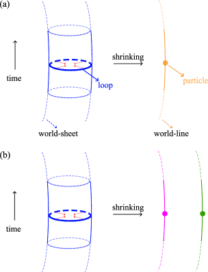
Figure 5: Illustration of the loop-shrinking operation. When a loop is shrunk to a particle, its world-sheet is shrunk to a line which turns out to be the world-line of the particle. In this situation, the integral of $2$-form gauge field in Wilson operator for loop excitation naturally vanishes, see Eq. (52) and the main text. (a) The outcome of loop shrinking operation can be a single particle. As shown in Table 6, shrinking an Abelian loop always results in one particle excitation. (b) The outcome of loop shrinking operation can also be a composite formed by multiple particles, e.g., the example of Eq. (53) discussed in the main text.

Table 6: Shrinking rules of topological excitations for BR topological order with $G=\left(\mathbb{Z}_{2}\right)^{3}$. The loop excitations are classified as Abelian and non-Abelian ones, depending on whether they have Abelian or non-Abelian fusion rules with other topological excitations. All these shrinking rules respect fusion rules, i.e., $\mathcal{S}\left(a\otimes b\right)=\mathcal{S}\left(a\right)\otimes\mathcal{S}\left(b\right)$, as explained in Sec. III.3. Shrinking an Abelian loop always results in an Abelian particle. On the other hand, shrinking a non-Abelian loop leads to either a non-Abelian particle or a composite particle (superposition of multiple simple particles).

Abelian loops	$\mathsf{L}_{001}$	$\mathsf{L}_{001}^{100}$	$\mathsf{L}_{001}^{010}$	$\mathsf{L}_{001}^{110}$
$\mathcal{S}\left(\textbf{Abelian loop}\right)$	$\mathsf{1}$	$\mathsf{P}_{100}$	$\mathsf{P}_{010}$	$\mathsf{P}_{110}$
non-Abelian loops	$\mathsf{L}_{100}$	$\mathsf{L}_{100}^{100}$	$\mathsf{L}_{010}$	$\mathsf{L}_{010}^{010}$	$\mathsf{L}_{001}^{001}$	$\mathsf{L}_{110}$	$\mathsf{L}_{110}^{100}$	$\mathsf{L}_{100}^{001}$	$\mathsf{L}_{010}^{001}$	$\mathsf{L}_{110}^{001}$
$\mathcal{S}\left(\textbf{non-Abelian loop}\right)$	$\mathsf{1}\oplus\mathsf{P}_{010}$	$\mathsf{P}_{100}\oplus\mathsf{P}_{110}$	$\mathsf{1}\oplus\mathsf{P}_{100}$	$\mathsf{P}_{010}\oplus\mathsf{P}_{110}$	$\mathsf{P}_{001}$	$\mathsf{1}\oplus\mathsf{P}_{110}$	$\mathsf{P}_{100}\oplus\mathsf{P}_{010}$	$2\cdot\mathsf{P}_{001}$	$2\cdot\mathsf{P}_{001}$	$2\cdot\mathsf{P}_{001}$

Physically, one may expect that the shrinking operation should respect the fusion rules:

$$\mathcal{S}\left(\mathsf{a}\otimes\mathsf{b}\right)=\mathcal{S}\left(\mathsf{a}\right)\otimes\mathcal{S}\left(\mathsf{b}\right)$$ (54)

where $\mathsf{a}$ and $\mathsf{b}$ are excitations. It is natural to set $\mathcal{S}\left(\mathsf{a}\right)=\mathsf{a}$ if $\mathsf{a}$ is a particle excitation. Analogous to fusion rules, we can write the shrinking rules in the form of

$$\mathcal{S}\left(\mathsf{a}\right)=\oplus_{\mathsf{c}}\mathrm{S}_{\mathsf{c}}^{\mathsf{a}}\cdot\mathsf{c}$$ (55)

where the non-zero integer $\mathrm{S}_{\mathsf{c}}^{\mathsf{a}}$ behaves as the “shrinking coefficient”. Using this notation, we have

$$\mathcal{S}\left(\mathsf{a}\otimes\mathsf{b}\right)= \mathcal{S}\left(\oplus_{\mathsf{c}}N_{\mathsf{c}}^{\mathsf{a}\mathsf{b}}\cdot\mathsf{c}\right)$$

$$= \sum_{\mathsf{c}}N_{\mathsf{c}}^{\mathsf{a}\mathsf{b}}\cdot\mathcal{S}\left(\mathsf{c}\right)$$

$$= \sum_{\mathsf{c}}N_{\mathsf{c}}^{\mathsf{a}\mathsf{b}}\cdot\oplus_{\mathsf{d}}\mathrm{S}_{\mathsf{d}}^{\mathsf{c}}\cdot\mathsf{d}$$

$$= \oplus_{\mathsf{d}}\left(\sum_{\mathsf{c}}N_{\mathsf{c}}^{\mathsf{a}\mathsf{b}}\mathrm{S}_{\mathsf{d}}^{\mathsf{c}}\right)\cdot\mathsf{d}$$ (56)

and

$$\mathcal{S}\left(\mathsf{a}\right)\otimes\mathcal{S}\left(\mathsf{b}\right)= \left(\oplus_{\mathsf{k_{1}}}\mathrm{S}_{\mathsf{k_{1}}}^{\mathsf{a}}\cdot\mathsf{k_{1}}\right)\otimes\left(\oplus_{\mathsf{k_{2}}}\mathrm{S}_{\mathsf{k_{2}}}^{\mathsf{b}}\cdot\mathsf{k_{2}}\right)$$

$$= \oplus_{\mathsf{k_{1}}}\mathrm{S}_{\mathsf{k_{1}}}^{\mathsf{a}}\cdot\oplus_{\mathsf{k_{2}}}\mathrm{S}_{\mathsf{k_{2}}}^{\mathsf{b}}\cdot\left(\mathsf{k_{1}}\otimes\mathsf{k_{2}}\right)$$

$$= \sum_{\mathsf{k_{1}}}\sum_{\mathsf{k_{2}}}\mathrm{S}_{\mathsf{k_{1}}}^{\mathsf{a}}\mathrm{S}_{\mathsf{k_{2}}}^{\mathsf{b}}\left(\oplus_{\mathsf{d}}N_{\mathsf{d}}^{\mathsf{k_{1}}\mathsf{k_{2}}}\cdot\mathsf{d}\right)$$

$$= \oplus_{\mathsf{d}}\left(\sum_{\mathsf{k_{1}},\mathsf{k_{2}}}\mathrm{S}_{\mathsf{k_{1}}}^{\mathsf{a}}\mathrm{S}_{\mathsf{k_{2}}}^{\mathsf{b}}N_{\mathsf{d}}^{\mathsf{k_{1}}\mathsf{k_{2}}}\right)\cdot\mathsf{d}.$$ (57)

By calculating the $N_{k}^{ij}$ and $\mathrm{S}_{c}^{a}$ data from Table 4 and Table 6, we confirm that for arbitrary excitations $\mathsf{a}$ and $\mathsf{b}$

$$\sum_{\mathsf{c}}N_{\mathsf{c}}^{\mathsf{a}\mathsf{b}}\mathrm{S}_{\mathsf{d}}^{\mathsf{c}}=\sum_{\mathsf{k_{1}},\mathsf{k_{2}}}\mathrm{S}_{\mathsf{k_{1}}}^{\mathsf{a}}\mathrm{S}_{\mathsf{k_{2}}}^{\mathsf{b}}N_{\mathsf{d}}^{\mathsf{k_{1}}\mathsf{k_{2}}}$$ (58)

is always satisfied, i.e., the shrinking rules respect the fusion rules as Eq. (54).

Furthermore, by taking a closer look at the loop shrinking rules in Table 6, we can conclude the following facts from our field-theoretical analysis:

1. The quantum dimensions of topological excitations are conserved under loop shrinking operation. This can be checked by referring to Table 5.

2. An Abelian loop is always shrunk into an Abelian particle. On the other hand, a non-Abelian loop is shrunk into either a non-Abelian particle or a composite particle.

3. The loop shrinking rules is consistent with fusion rules, i.e., $\mathcal{S}\left(\mathsf{a}\otimes\mathsf{b}\right)=\mathcal{S}\left(\mathsf{a}\right)\otimes\mathcal{S}\left(\mathsf{b}\right)$.

All these facts indicate the consistency of fusion rules and loop shrinking rules. We believe that this consistency of fusion rules and loop shrinking rules play an important role in establishing an anomaly-free topological order. A quantum anomaly may occur if the loop shrinking rules conflict with fusion rules, which is an interesting future direction for field theory study.

IV Fusion rules of topological orders with compatible braidings in $3$D space

Though braiding processes in topological order can be described by TQFT in a unified framework, not all of them can be supported in one system without incompatibility (Zhang and Ye, 2021). For a given gauge group, different topological order can be obtained according to different combinations of compatible braiding processes. In this section we would like to answer this question: how the fusion rules of topological order differ depending on the combination of compatible braidings.

In $3$D space, nontrivial braiding processes in $3$D space include particle-loop braiding, multi-loop braiding, and Borromean rings braiding. Yet not arbitrary combination of these braiding processes are compatible. For example, when the gauge group is $G=\prod_{i=1}^{3}\mathbb{Z}_{N_{i}}$, the Borromean rings braiding can be compatible with three-loop braiding, if the loops in $3$-loop braiding only carry two kinds of $\mathbb{Z}_{N_{i}}$ fluxes. If these three loops carry three kinds of $\mathbb{Z}_{N_{i}}$ fluxes, the $3$-loop braiding is not compatible with the Borromean rings braiding. The origin of this incompatibility is that we cannot construct a gauge-invariant TQFT action for these two braiding processes (Zhang and Ye, 2021).

Below, we study the fusion rules for topological order with particle-loop braiding only, with particle-loop braiding and $3$-loop braiding, and with all three kinds of braiding processes, respectively. We find that for topological orders with particle-loop braidings and $3$-loop braidings only, the fusion rules are Abelian. However, once we introduce Borromean rings braiding, the fusion rules become non-Abelian.

IV.1 Topological order with particle-loop braiding only: $G=\left(\mathbb{Z}_{2}\right)^{2}$

The TQFT action for topological order with particle-loop braiding only is

$$S=S_{BF}=\int\sum_{i=1}^{2}\frac{N_{i}}{2\pi}B^{i}dA^{i}.$$ (59)

Since $G=\left(\mathbb{Z}_{2}\right)^{2}$, $N_{1}=N_{2}=2$. The gauge transformations are

$$A^{i}\rightarrow A^{i}+d\chi^{i},$$ (60)

$$B^{i}\rightarrow B^{i}+dV^{i}.$$

Particle excitations are represented by operators

$$\mathsf{P}_{ij}=\exp\left({\rm i}i\int_{\gamma}A^{1}+{\rm i}j\int_{\gamma}A^{2}\right)$$ (61)

with $i,j=0,1$. Loop excitations are represented by

$$\mathsf{L}_{10}^{ij}=\exp\left({\rm i}\int_{\sigma}B^{1}+{\rm i}i\int_{\gamma}A^{1}+{\rm i}j\int_{\gamma}A^{2}\right),$$ (62)

$$\mathsf{L}_{01}^{ij}=\exp\left({\rm i}\int_{\sigma}B^{2}+{\rm i}i\int_{\gamma}A^{1}+{\rm i}j\int_{\gamma}A^{2}\right),$$ (63)

$$\mathsf{L}_{11}^{ij}=\exp\left({\rm i}\int_{\sigma}B^{1}+{\rm i}\int_{\sigma}B^{2}+{\rm i}i\int_{\gamma}A^{1}+{\rm i}j\int_{\gamma}A^{2}\right),$$ (64)

with $i,j=0,1$. The fusion rules for these excitations are summarized in Table 7. These fusion rules, being Abelian, form a $\left(\mathbb{Z}_{2}\right)^{4}$ group.

Table 7: Fusion table for $S=S_{BF}$, $S=S_{BF}+S_{A^{1}A^{2}dA^{2}}$, or $S=S_{BF}+S_{A^{1}A^{2}dA^{2}}+S_{A^{2}A^{1}dA^{1}}$ with $G=\mathbb{Z}_{2}\times\mathbb{Z}_{2}$. For different TQFT actions (see Sec. IV.1, IV.2 and IV.3), the same notation $\mathsf{P}_{n_{1}n_{2}}$ or $\mathsf{L}_{n_{1}n_{2}}^{c_{1}c_{2}}$ represents the same excitation though the expression of Wilson operator depends on the gauge transformations. For example, $\mathsf{L}_{10}$ denotes the loop carrying $\mathbb{Z}_{N_{1}}$ flux yet its explicit operator expression varies for different TQFT actions, as shown in Sec. IV.1, IV.2 and IV.3. All fusion rules are Abelian hence the quantum dimension of each excitation is $1$. The fusions of all $16$ excitations form a $\left(\mathbb{Z}_{2}\right)^{4}$ group.

$\mathsf{P}_{00}\equiv\mathsf{1}$

$\mathsf{P}_{10}$

$\mathsf{P}_{01}$

$\mathsf{P}_{11}$

$\mathsf{L}_{10}$

$\mathsf{L}_{01}$

$\mathsf{L}_{11}$

$\mathsf{L}_{10}^{10}$

$\mathsf{L}_{01}^{10}$

$\mathsf{L}_{11}^{10}$

$\mathsf{L}_{10}^{01}$

$\mathsf{L}_{01}^{01}$

$\mathsf{L}_{11}^{01}$

$\mathsf{L}_{10}^{11}$

$\mathsf{L}_{01}^{11}$

$\mathsf{L}_{11}^{11}$

$\mathsf{1}$

$\mathsf{1}$

$\mathsf{P}_{10}$

$\mathsf{P}_{01}$

$\mathsf{P}_{11}$

$\mathsf{L}_{10}$

$\mathsf{L}_{01}$

$\mathsf{L}_{11}$

$\mathsf{L}_{10}^{10}$

$\mathsf{L}_{01}^{10}$

$\mathsf{L}_{11}^{10}$

$\mathsf{L}_{10}^{01}$

$\mathsf{L}_{01}^{01}$

$\mathsf{L}_{11}^{01}$

$\mathsf{L}_{10}^{11}$

$\mathsf{L}_{01}^{11}$

$\mathsf{L}_{11}^{11}$

$\mathsf{P}_{10}$

$\mathsf{P}_{10}$

$\mathsf{1}$

$\mathsf{P}_{11}$

$\mathsf{P}_{01}$

$\mathsf{L}_{10}^{10}$

$\mathsf{L}_{01}^{10}$

$\mathsf{L}_{11}^{10}$

$\mathsf{L}_{10}$

$\mathsf{L}_{01}$

$\mathsf{L}_{11}$

$\mathsf{L}_{10}^{11}$

$\mathsf{L}_{01}^{11}$

$\mathsf{L}_{11}^{11}$

$\mathsf{L}_{10}^{01}$

$\mathsf{L}_{01}^{01}$

$\mathsf{L}_{11}^{01}$

$\mathsf{P}_{01}$

$\mathsf{P}_{01}$

$\mathsf{P}_{11}$

$\mathsf{1}$

$\mathsf{P}_{10}$

$\mathsf{L}_{10}^{01}$

$\mathsf{L}_{01}^{01}$

$\mathsf{L}_{11}^{01}$

$\mathsf{L}_{10}^{11}$

$\mathsf{L}_{01}^{11}$

$\mathsf{L}_{11}^{11}$

$\mathsf{L}_{10}$

$\mathsf{L}_{01}$

$\mathsf{L}_{11}$

$\mathsf{L}_{10}^{10}$

$\mathsf{L}_{01}^{10}$

$\mathsf{L}_{11}^{10}$

$\mathsf{P}_{11}$

$\mathsf{P}_{11}$

$\mathsf{P}_{01}$

$\mathsf{P}_{10}$

$\mathsf{1}$

$\mathsf{L}_{10}^{11}$

$\mathsf{L}_{01}^{11}$

$\mathsf{L}_{11}^{11}$

$\mathsf{L}_{10}^{01}$

$\mathsf{L}_{01}^{01}$

$\mathsf{L}_{11}^{01}$

$\mathsf{L}_{10}^{10}$

$\mathsf{L}_{01}^{10}$

$\mathsf{L}_{11}^{10}$

$\mathsf{L}_{10}$

$\mathsf{L}_{01}$

$\mathsf{L}_{11}$

$\mathsf{L}_{10}$

$\mathsf{L}_{10}$

$\mathsf{L}_{10}^{10}$

$\mathsf{L}_{10}^{01}$

$\mathsf{L}_{10}^{11}$

$\mathsf{1}$

$\mathsf{L}_{11}$

$\mathsf{L}_{01}$

$\mathsf{P}_{10}$

$\mathsf{L}_{11}^{10}$

$\mathsf{L}_{01}^{10}$

$\mathsf{P}_{01}$

$\mathsf{L}_{11}^{01}$

$\mathsf{L}_{01}^{01}$

$\mathsf{P}_{11}$

$\mathsf{L}_{11}^{11}$

$\mathsf{L}_{01}^{11}$

$\mathsf{L}_{01}$

$\mathsf{L}_{01}$

$\mathsf{L}_{01}^{10}$

$\mathsf{L}_{01}^{01}$

$\mathsf{L}_{01}^{11}$

$\mathsf{L}_{11}$

$\mathsf{1}$

$\mathsf{L}_{10}$

$\mathsf{L}_{11}^{10}$

$\mathsf{P}_{10}$

$\mathsf{L}_{10}^{10}$

$\mathsf{L}_{11}^{01}$

$\mathsf{P}_{01}$

$\mathsf{L}_{10}^{01}$

$\mathsf{L}_{11}^{11}$

$\mathsf{P}_{11}$

$\mathsf{L}_{10}^{11}$

$\mathsf{L}_{11}$

$\mathsf{L}_{11}$

$\mathsf{L}_{11}^{10}$

$\mathsf{L}_{11}^{01}$

$\mathsf{L}_{11}^{11}$

$\mathsf{L}_{01}$

$\mathsf{L}_{10}$

$\mathsf{1}$

$\mathsf{L}_{01}^{10}$

$\mathsf{L}_{10}^{10}$

$\mathsf{P}_{10}$

$\mathsf{L}_{01}^{01}$

$\mathsf{L}_{10}^{01}$

$\mathsf{P}_{01}$

$\mathsf{L}_{01}^{11}$

$\mathsf{L}_{10}^{11}$

$\mathsf{P}_{11}$

$\mathsf{L}_{10}^{10}$

$\mathsf{L}_{10}^{10}$

$\mathsf{L}_{10}$

$\mathsf{L}_{10}^{11}$

$\mathsf{L}_{10}^{01}$

$\mathsf{P}_{10}$

$\mathsf{L}_{11}^{10}$

$\mathsf{L}_{01}^{10}$

$\mathsf{1}$

$\mathsf{L}_{11}$

$\mathsf{L}_{01}$

$\mathsf{P}_{11}$

$\mathsf{L}_{11}^{11}$

$\mathsf{L}_{01}^{11}$

$\mathsf{P}_{01}$

$\mathsf{L}_{11}^{01}$

$\mathsf{L}_{01}^{01}$

$\mathsf{L}_{01}^{10}$

$\mathsf{L}_{01}^{10}$

$\mathsf{L}_{01}$

$\mathsf{L}_{01}^{11}$

$\mathsf{L}_{01}^{01}$

$\mathsf{L}_{11}^{10}$

$\mathsf{P}_{10}$

$\mathsf{L}_{10}^{10}$

$\mathsf{L}_{11}$

$\mathsf{1}$

$\mathsf{L}_{10}$

$\mathsf{L}_{11}^{11}$

$\mathsf{P}_{11}$

$\mathsf{L}_{10}^{11}$

$\mathsf{L}_{11}^{01}$

$\mathsf{P}_{01}$

$\mathsf{L}_{10}^{01}$

$\mathsf{L}_{11}^{10}$

$\mathsf{L}_{11}^{10}$

$\mathsf{L}_{11}$

$\mathsf{L}_{11}^{11}$

$\mathsf{L}_{11}^{01}$

$\mathsf{L}_{01}^{10}$

$\mathsf{L}_{10}^{10}$

$\mathsf{P}_{10}$

$\mathsf{L}_{01}$

$\mathsf{L}_{10}$

$\mathsf{1}$

$\mathsf{L}_{01}^{11}$

$\mathsf{L}_{10}^{11}$

$\mathsf{P}_{11}$

$\mathsf{L}_{01}^{01}$

$\mathsf{L}_{10}^{01}$

$\mathsf{P}_{01}$

$\mathsf{L}_{10}^{01}$

$\mathsf{L}_{10}^{01}$

$\mathsf{L}_{10}^{11}$

$\mathsf{L}_{10}$

$\mathsf{L}_{10}^{10}$

$\mathsf{P}_{01}$

$\mathsf{L}_{11}^{01}$

$\mathsf{L}_{01}^{01}$

$\mathsf{P}_{11}$

$\mathsf{L}_{11}^{11}$

$\mathsf{L}_{01}^{11}$

$\mathsf{1}$

$\mathsf{L}_{11}$

$\mathsf{L}_{01}$

$\mathsf{P}_{10}$

$\mathsf{L}_{11}^{10}$

$\mathsf{L}_{01}^{10}$

$\mathsf{L}_{01}^{01}$

$\mathsf{L}_{01}^{01}$

$\mathsf{L}_{01}^{11}$

$\mathsf{L}_{01}$

$\mathsf{L}_{01}^{10}$

$\mathsf{L}_{11}^{01}$

$\mathsf{P}_{01}$

$\mathsf{L}_{10}^{01}$

$\mathsf{L}_{11}^{11}$

$\mathsf{P}_{11}$

$\mathsf{L}_{10}^{11}$

$\mathsf{L}_{11}$

$\mathsf{1}$

$\mathsf{L}_{10}$

$\mathsf{L}_{11}^{10}$

$\mathsf{P}_{10}$

$\mathsf{L}_{10}^{10}$

$\mathsf{L}_{11}^{01}$

$\mathsf{L}_{11}^{01}$

$\mathsf{L}_{11}^{11}$

$\mathsf{L}_{11}$

$\mathsf{L}_{11}^{10}$

$\mathsf{L}_{01}^{01}$

$\mathsf{L}_{10}^{01}$

$\mathsf{P}_{01}$

$\mathsf{L}_{01}^{11}$

$\mathsf{L}_{10}^{11}$

$\mathsf{P}_{11}$

$\mathsf{L}_{01}$

$\mathsf{L}_{10}$

$\mathsf{1}$

$\mathsf{L}_{01}^{10}$

$\mathsf{L}_{10}^{10}$

$\mathsf{P}_{10}$

$\mathsf{L}_{10}^{11}$

$\mathsf{L}_{10}^{11}$

$\mathsf{L}_{10}^{01}$

$\mathsf{L}_{10}^{10}$

$\mathsf{L}_{10}$

$\mathsf{P}_{11}$

$\mathsf{L}_{11}^{11}$

$\mathsf{L}_{01}^{11}$

$\mathsf{P}_{01}$

$\mathsf{L}_{11}^{01}$

$\mathsf{L}_{01}^{01}$

$\mathsf{P}_{10}$

$\mathsf{L}_{11}^{10}$

$\mathsf{L}_{01}^{10}$

$\mathsf{1}$

$\mathsf{L}_{11}$

$\mathsf{L}_{01}$

$\mathsf{L}_{01}^{11}$

$\mathsf{L}_{01}^{11}$

$\mathsf{L}_{01}^{01}$

$\mathsf{L}_{01}^{10}$

$\mathsf{L}_{01}$

$\mathsf{L}_{11}^{11}$

$\mathsf{P}_{11}$

$\mathsf{L}_{10}^{11}$

$\mathsf{L}_{11}^{01}$

$\mathsf{P}_{01}$

$\mathsf{L}_{10}^{01}$

$\mathsf{L}_{11}^{10}$

$\mathsf{P}_{10}$

$\mathsf{L}_{10}^{10}$

$\mathsf{L}_{11}$

$\mathsf{1}$

$\mathsf{L}_{10}$

$\mathsf{L}_{11}^{11}$

$\mathsf{L}_{11}^{11}$

$\mathsf{L}_{11}^{01}$

$\mathsf{L}_{11}^{10}$

$\mathsf{L}_{11}$

$\mathsf{L}_{01}^{11}$

$\mathsf{L}_{10}^{11}$

$\mathsf{P}_{11}$

$\mathsf{L}_{01}^{01}$

$\mathsf{L}_{10}^{01}$

$\mathsf{P}_{01}$

$\mathsf{L}_{01}^{10}$

$\mathsf{L}_{10}^{10}$

$\mathsf{P}_{10}$

$\mathsf{L}_{01}$

$\mathsf{L}_{10}$

$\mathsf{1}$

IV.2 Topological order with particle-loop braiding and $3$-loop braiding: $G=\left(\mathbb{Z}_{2}\right)^{2}$

The TQFT action for topological order with particle-loop braiding and $3$-loop braiding is

$$S= S_{BF}+S_{A^{1}A^{2}dA^{2}}$$

$$= \sum_{i=1}^{2}\frac{N_{i}}{2\pi}B^{i}dA^{i}+\frac{pN_{1}N_{2}}{\left(2\pi\right)^{2}N_{12}}A^{1}A^{2}dA^{2}$$ (65)

with $N_{1}=N_{2}=2$, $N_{12}\equiv\gcd\left(N_{1},N_{2}\right)=2$ and $p\in\mathbb{Z}_{N_{12}}$. For a nontrivial action, we can set $p=1$. The gauge transformations are

$$A^{i}\rightarrow A^{i}+d\chi^{i},$$ (66)

$$B^{1}\rightarrow B^{1}+dV^{1}+\frac{pN_{2}}{2\pi N_{12}}d\chi^{2}A^{2},$$ (67)

$$B^{2}\rightarrow B^{2}+dV^{2}-\frac{pN_{1}}{2\pi N_{12}}d\chi^{1}A^{2}.$$ (68)

Particle excitations are represented by operators

$$\mathsf{P}_{ij}=\exp\left({\rm i}i\int_{\gamma}A^{1}+{\rm i}j\int_{\gamma}A^{2}\right)$$ (69)

with $i,j=0,1$. Loop excitations are represented by

$$\mathsf{L}_{10}^{ij}= \exp\left[{\rm i}\left(\int_{\sigma}B^{1}+\frac{pN_{2}}{2\pi N_{12}}\int_{\Omega}A^{2}dA^{2}\right)\right.$$

$$+\left.{\rm i}i\int_{\gamma}A^{1}+{\rm i}j\int_{\gamma}A^{2}\right],$$ (70)

$$\mathsf{L}_{01}^{ij}= \exp\left[{\rm i}\left(\int_{\sigma}B^{2}-\frac{pN_{1}}{2\pi N_{12}}\int_{\Omega}A^{1}dA^{2}\right)\right.$$

$$+\left.{\rm i}i\int_{\gamma}A^{1}+{\rm i}j\int_{\gamma}A^{2}\right],$$ (71)

$$\mathsf{L}_{11}^{ij}= \exp\left[{\rm i}\left(\int_{\sigma}B^{1}+\frac{pN_{2}}{2\pi N_{12}}\int_{\Omega}A^{2}dA^{2}\right)\right.$$

$$+{\rm i}\left(\int_{\sigma}B^{2}-\frac{pN_{1}}{2\pi N_{12}}\int_{\Omega}A^{1}dA^{2}\right)$$

$$+\left.{\rm i}i\int_{\gamma}A^{1}+{\rm i}j\int_{\gamma}A^{2}\right],$$ (72)

with $i,j=0,1$. There are $2^{4}=16$ nonequivalent excitations in total. Using the field-theoretical approach developed in Sec. III, we find that the fusion rules in this case are the same as those of $S=S_{BF}$ with $G=\mathbb{Z}_{2}\times\mathbb{Z}_{2}$. In other words, the fusion rules in this case are also shown in Table. 7.

IV.3 Topological order with particle-loop braiding and two different $3$-loop braidings: $G=\left(\mathbb{Z}_{2}\right)^{2}$

The TQFT action $S=S_{BF}+S_{A^{1}A^{2}dA^{2}}+S_{A^{2}A^{1}dA^{1}}$ describes the topological order with particle-loop braiding and two different but compatible $3$-loop braidings. The action is

$$S= \int\sum_{i=1}^{2}\frac{N_{i}}{2\pi}B^{i}dA^{i}$$

$$+\frac{p_{1}N_{1}N_{2}}{\left(2\pi\right)^{2}N_{12}}A^{1}A^{2}dA^{2}+\frac{p_{2}N_{1}N_{2}}{\left(2\pi\right)^{2}N_{12}}A^{2}A^{1}dA^{1}$$ (73)

with $N_{1}=N_{2}=2$, $N_{12}\equiv\gcd\left(N_{1},N_{2}\right)=2$ and $p_{1}p_{2}\in\mathbb{Z}_{N_{12}}$. We can view this action as the stack of $S=S_{BF}+S_{A^{1}A^{2}dA^{2}}$ and $S=S_{BF}+S_{A^{2}A^{1}dA^{1}}$. The gauge transformations are

$$A^{i}\rightarrow A^{i}+d\chi^{i},$$ (74)

$$B^{1}\rightarrow B^{1}+dV^{1}+\frac{p_{1}N_{2}}{2\pi N_{12}}d\chi^{2}A^{2}-\frac{p_{2}N_{2}}{2\pi N_{12}}d\chi^{2}A^{1},$$ (75)

$$B^{2}\rightarrow B^{2}+dV^{2}-\frac{p_{1}N_{1}}{2\pi N_{12}}d\chi^{1}A^{2}+\frac{p_{2}N_{1}}{2\pi N_{12}}d\chi^{1}A^{1}.$$ (76)

The particle and loop (including pure loop and decorated loop) excitations are represented by the following operators:

$$\mathsf{P}_{ij}=\exp\left({\rm i}i\int_{\gamma}A^{1}+{\rm i}j\int_{\gamma}A^{2}\right),$$ (77)

$$\mathsf{L}_{10}^{ij}$$

$$= \exp\left[{\rm i}\left(\int_{\sigma}B^{1}+\frac{p_{1}N_{2}}{2\pi N_{12}}\int_{\Omega}A^{2}dA^{2}-\frac{p_{2}N_{2}}{2\pi N_{12}}\int_{\Omega}A^{2}dA^{1}\right)\right.$$

$$+\left.{\rm i}i\int_{\gamma}A^{1}+{\rm i}j\int_{\gamma}A^{2}\right],$$ (78)

$$\mathsf{L}_{01}^{ij}$$

$$= \exp\left[{\rm i}\left(\int_{\sigma}B^{2}-\frac{p_{1}N_{1}}{2\pi N_{12}}\int_{\Omega}A^{1}dA^{2}+\frac{p_{2}N_{1}}{2\pi N_{12}}\int_{\Omega}A^{1}dA^{1}\right)\right.$$

$$+\left.{\rm i}i\int_{\gamma}A^{1}+{\rm i}j\int_{\gamma}A^{2}\right],$$ (79)

$$\mathsf{L}_{11}^{ij}$$

$$= \exp\left[{\rm i}\left(\int_{\sigma}B^{1}+\frac{pN_{2}}{2\pi N_{12}}\int_{\Omega}A^{2}dA^{2}-\frac{p_{2}N_{2}}{2\pi N_{12}}\int_{\Omega}A^{2}dA^{1}\right)\right.$$

$$+{\rm i}\left(\int_{\sigma}B^{2}-\frac{pN_{1}}{2\pi N_{12}}\int_{\Omega}A^{1}dA^{2}+\frac{p_{2}N_{1}}{2\pi N_{12}}\int_{\Omega}A^{1}dA^{1}\right)$$

$$+\left.{\rm i}i\int_{\gamma}A^{1}+{\rm i}j\int_{\gamma}A^{2}\right],$$ (80)

where $i,j=0,1$. The number of all nonequivalent excitations is $16$. Again, we find fusion rules in this case same as those of $S=S_{BF}$ with $G=\mathbb{Z}_{2}\times\mathbb{Z}_{2}$, i.e., shown in Table. 7. Combining the discussion in Sec. IV.1, IV.2 and IV.3, we can conclude that when $G=\mathbb{Z}_{2}\times\mathbb{Z}_{2}$ the fusion rules of excitations are unchanged, forming a $\left(\mathbb{Z}_{2}\right)^{4}$ group, no matter the TQFT action contains twisted terms or not. In other words, with $G=\mathbb{Z}_{2}\times\mathbb{Z}_{2}$, the fusion rules of different topologically ordered systems which support different but mutually compatible braidings are same.

IV.4 Topological order with particle-loop braiding and $3$-loop braiding: $G=\left(\mathbb{Z}_{2}\right)^{3}$

When $G=\prod_{i=1}^{3}\mathbb{Z}_{N_{i}}$, the TQFT action for topological order with particle-loop braiding and $3$-loop braiding can be

$$S =S_{BF}+S_{A^{1}A^{2}dA^{3}}$$

$$=\int\sum_{i=1}^{3}\frac{N_{i}}{2\pi}B^{i}dA^{i}+\frac{pN_{1}N_{2}}{\left(2\pi\right)^{2}N_{12}}A^{1}A^{2}dA^{3}$$ (81)

with $N_{1}=N_{2}=N_{3}=2$, $N_{12}=2$, and $p\in\mathbb{Z}_{N_{12}}$, i.e., $p\in\mathbb{Z}_{2}$. We set $p=1$ so that the action is nontrivial:

$$S=\int\sum_{i=1}^{3}\frac{N_{i}}{2\pi}B^{i}dA^{i}+\frac{2}{\left(2\pi\right)^{2}}A^{1}A^{2}dA^{3}.$$ (82)

The gauge transformations are

$$A^{i}\rightarrow A^{i}+d\chi^{i},$$ (83)

$$B^{1}\rightarrow B^{1}+dV^{1}+\frac{pN_{2}}{2\pi N_{12}}d\chi^{2}A^{3},$$ (84)

$$B^{2}\rightarrow B^{2}+dV^{2}-\frac{pN_{1}}{2\pi N_{12}}d\chi^{1}A^{3},$$ (85)

$$B^{3}\rightarrow B^{3}+dV^{3}.$$ (86)

In this case, the particle excitations are represented by

$$\mathsf{P}_{ijl}=\exp\left({\rm i}i\int_{\gamma}A^{1}+{\rm i}j\int_{\gamma}A^{2}+{\rm i}k\int_{\gamma}A^{3}\right)$$ (87)

with $i,j,k=0,1$. The loop (pure loop and decorated loop) excitations are represented by the following Wilson operators:

$$\mathsf{L}_{100}^{ijl}= \exp\left({\rm i}\int_{\sigma}B^{1}+{\rm i}\frac{pN_{2}}{2\pi N_{12}}\int_{\Omega}A^{2}dA^{3}\right.$$

$$\left.+{\rm i}i\int_{\gamma}A^{1}+{\rm i}j\int_{\gamma}A^{2}+{\rm i}k\int_{\gamma}A^{3}\right),$$ (88)

$$\mathsf{L}_{010}^{ijl}= \exp\left({\rm i}\int_{\sigma}B^{1}+{\rm i}\frac{pN_{2}}{2\pi N_{12}}\int_{\Omega}A^{2}dA^{3}\right.$$

$$\left.+{\rm i}i\int_{\gamma}A^{1}+{\rm i}j\int_{\gamma}A^{2}+{\rm i}k\int_{\gamma}A^{3}\right),$$ (89)

$$\mathsf{L}_{001}^{ijl}= \exp\left({\rm i}\int_{\sigma}B^{3}\right.$$

$$\left.+{\rm i}i\int_{\gamma}A^{1}+{\rm i}j\int_{\gamma}A^{2}+{\rm i}k\int_{\gamma}A^{3}\right),$$ (90)

where $i,j,k=0,1$. Similarly, we find that the fusion rules of these excitations form a $\left(\mathbb{Z}_{2}\right)^{6}$ group. In addition, $S=S_{BF}+S_{AAdA}$ with arbitrary $AAdA$ twisted term produces identical fusion rules as $S=S_{BF}$ when $G=\left(\mathbb{Z}_{2}\right)^{{}^{3}}$. This is also true when $G=\mathbb{Z}_{2}\times\mathbb{Z}_{2}$ (see Sec. IV.1, IV.2 and IV.3). These results lead to the general conclusion: once given the gauge group $G=\prod_{i}\mathbb{Z}_{N_{i}}$, for different topologically ordered systems which support particle-loop braidings and/or $3$-loop braidings only, the fusion rules are same: they are Abelian and constitute a $\left(\prod_{i}\mathbb{Z}_{N_{i}}\right)^{2}$ group.

IV.5 Topological order with particle-loop braiding, $3$-loop braiding, and BR braiding: $G=\left(\mathbb{Z}_{2}\right)^{3}$

The Borromean rings braiding described by $S_{A^{1}A^{2}B^{3}}$ is compatible with the $3$-loop braiding described by $S_{A^{1}A^{2}dA^{2}}$ (Zhang and Ye, 2021). The TQFT action is given by

$$S= \int\sum_{i=1}^{3}\frac{N_{i}}{2\pi}B^{i}dA^{i}$$

$$+\frac{p_{1}N_{1}N_{2}}{\left(2\pi\right)^{2}N_{12}}A^{1}A^{2}dA^{2}+\frac{p_{2}N_{1}N_{2}N_{3}}{\left(2\pi\right)^{2}N_{123}}A^{1}A^{2}B^{3}$$ (91)

with $p_{1}\in\mathbb{Z}_{N_{12}}$ and $p_{2}\in\mathbb{Z}_{N_{123}}$. We set $p_{1}=p_{2}=1$. The gauge transformations are

$$A^{1}\rightarrow A^{1}+d\chi^{1},$$ (92)

$$A^{2}\rightarrow A^{2}+d\chi^{2},$$ (93)

$$A^{3}\rightarrow A^{3}+d\chi^{3}$$

$$-\frac{p_{2}N_{1}N_{2}}{2\pi N_{123}}\left(\chi^{1}A^{2}+\frac{1}{2}\chi^{1}d\chi^{2}\right)$$

$$+\frac{p_{2}N_{1}N_{2}}{2\pi N_{123}}\left(\chi^{2}A^{1}+\frac{1}{2}\chi^{2}d\chi^{1}\right),$$ (94)

$$B^{1}\rightarrow B^{1}+dV^{1}$$

$$+\frac{p_{1}N_{2}}{2\pi N_{12}}d\chi^{2}A^{2}$$

$$-\frac{p_{2}N_{2}N_{3}}{2\pi N_{123}}\left(\chi^{2}B^{3}-A^{2}V^{3}+\chi^{2}dV^{3}\right),$$ (95)

$$B^{2}\rightarrow B^{2}+dV^{2}$$

$$-\frac{p_{2}N_{1}}{2\pi N_{12}}d\chi^{1}A^{2}$$

$$+\frac{p_{2}N_{1}N_{3}}{2\pi N_{123}}\left(\chi^{1}B^{3}-A^{1}V^{3}+\chi^{1}dV^{3}\right),$$ (96)

$$B^{3}\rightarrow B^{3}+dV^{3}.$$ (97)

The loop and particle excitations are represented by operators shown in Table. 8 and Table. 9. We find these operators have a similar expression of those for $S=S_{BF}+S_{A^{1}A^{2}B^{3}}$, i.e., Eq. (1). In Sec. III we have seen that non-Abelian fusion can be traced back to the Kronecker delta function in operators. By performing similar calculation, we find that the operators listed in Table 9 and Table 8 obey the same fusion rules of $S=S_{BF}+S_{A^{1}A^{2}B^{3}}$, i.e., those shown in Table 4. This result is different from those of $S=S_{BF}$ and $S=S_{BF}+S_{AAdA}$ aforementioned. As pointed out in Ref. (Zhang and Ye, 2021), BR braiding is not always compatible with multi-loop braidings. If a BR braiding is introduced compatibly to a system that only supports particle-loop braiding and/or multi-loop braiding only, the formerly Abelian fusion rules would be dramatically changed to be non-Abelian.

V Discussion and outlook

In this work, we perform field-theoretical analysis on Wilson operators (i.e., the excitation contents), fusion rules, and loop-shrinking rules in three dimensional topological orders. Let us briefly review this paper. First, gauge-invariant Wilson operators are written down for nonequivalent topological excitations. The number of particle excitations and pure loop excitations agrees with that calculated from a lattice cocycle model. Next, fusion rules are represented in terms of path integral of TQFT and we find out all fusion rules as well as quantum dimensions. Some of the fusion rules are non-Abelian though the input gauge group for this topological order is Abelian. Beside the fusion rules, we also study the shrinking rules of loop excitations, which is a very interesting topological property of spatially nonlocal topological excitations. We propose a field-theoretical framework to perform the shrinking operation in terms of operators and path integral, i.e, shrinking the loop’s world-sheet to a world-line. The loop shrinking rules obtained are consistent with fusion rules, i.e., they respect fusion rules and conserve the quantum dimensions through the shrinking process. The consistency between fusion rules and loop-shrinking rules is critical in establishing an anomaly-free topological order in 3D. Motivated by the present work, we expect to explore the following topics in the near future.

i.—We expect more field-theoretical calculations may give a hint on the consistency among braiding data, fusion rules and shrinking rules in general 3D topological orders. Once inconsistency happens, the corresponding topological orders might be potentially anomalous and only realizable on the boundary of some 4D topological phases of matter.

ii.—It will be interesting to attempt to understand the algebraic structure behind the fusion rules of Borromean rings topological order and all topological orders with compatible braidings discussed in this paper. Considering that the BR topological order is beyond the usual DW gauge theory (Moradi and Wen, 2015; Lan et al., 2018; Bullivant and Delcamp, 2019, 2021, 2022) classification, it may be described by the generalized Drinfel’d center (a braided monoidal 2-category) of a 2-group (a special kind of fusion 2-category). In addition, our theory finds that, fusing a loop and its anti-loop may generate a fusion channel with two vacua. This is very unusual since in 2D topological orders, fusing a particle and its anti-particle must only have one vacuum. We conjecture this phenomenon may be related to the incorporation of “2-group” structure in our field theory, which is absent in field-theory of 2D topological order. In summary, the goal of this paper is to construct a field-theoretical study, more precisely, the path-integral calculation on topological invariants; the corresponding algebraic description is also important, which will be one of future directions.

iii.—It will be important to generalize the classification of Abelian symmetry fractionalization in Ref. Ning et al. (2022) to BR topological order as well as all other topological orders with compatible braidings, which leads to a more complete field-theoretical understanding on Symmetry Enriched Topological phases in 3D Ning et al. (2022, 2016); Ye (2018) and thus generalize Table I of Ref. Ning et al. (2022) to non-Abelian fractionalization.

iv.—Just like the study of non-Abelian anyons in 2D topological systems, braiding, fusion, and shrinking are topological invariants are vital in theory of TQC of higher dimensional stabilizer codes. So, we expect that our field-theoretical study will be helpful along this line of efforts, especially on the roles of loop-like excitations (errors/defects).

v.—It will be curious to ask what is the physical consequence of knotted loops or mutually linked loops when performing fusion or shrinking operations. Our field-theoretical study has provided concrete procedures for computation of unknotted loops, which in principle can be applied to more complicated loops. We leave these exciting questions for future exploration.

Table 8: Operators for nonequivalent loop excitations in $S=S_{BF}+S_{A^{1}A^{2}dA^{2}}+S_{A^{1}A^{2}B^{3}}$ with $G=\left(\mathbb{Z}_{2}\right)^{3}$ (see Sec. IV.5). Among them, there are $1$ trivial loop, $4$ nontrivial pure loops and $10$ decorated loops. The “$0$ or $\mathbb{Z}_{N_{i}}$” charge decoration means that the operator of pure loop (no particle attached to it) is equivalent to that of the loop decorated with a particle carrying $\mathbb{Z}_{N_{i}}$ gauge charge. The equivalence operators are explained in Sec. II.2.

Fluxes	Charge decoration	Operators for loop excitations	Equivalent operators
$0$	$0$	$\mathsf{L}_{000}=\mathsf{1}=\exp\left({\rm i}0\right)=1$	-
$\mathbb{Z}_{N_{1}}$	$0$ or $\mathbb{Z}_{N_{2}}$	$\begin{aligned} \mathsf{L}_{100}=&2\exp\left[{\rm i}\int_{\sigma}B^{1}+\frac{1}{2}\frac{2\pi q}{N_{1}}\left(d^{-1}A^{2}B^{3}+d^{-1}B^{3}A^{2}\right)+{\rm i}\int_{\Omega}\frac{p_{1}N_{2}}{2\pi N_{12}}A^{2}dA^{2}\right]\\ &\times\delta\left(\int_{\gamma}A^{2}\right)\delta\left(\int_{\sigma}B^{3}\right)\end{aligned}$	$\mathsf{L}_{100}=\mathsf{L}_{10n_{3}}^{0c_{2}0};c_{2},n_{3}=0,1$
$\mathbb{Z}_{N_{1}}$	$\mathbb{Z}_{N_{1}}$	$\begin{aligned} \mathsf{L}_{100}^{100}=&2\exp\left[{\rm i}\int_{\gamma}A^{1}+{\rm i}\int_{\sigma}B^{1}+\frac{1}{2}\frac{2\pi q}{N_{1}}\left(d^{-1}A^{2}B^{3}+d^{-1}B^{3}A^{2}\right)+{\rm i}\int_{\Omega}\frac{p_{1}N_{2}}{2\pi N_{12}}A^{2}dA^{2}\right]\\ &\times\delta\left(\int_{\gamma}A^{2}\right)\delta\left(\int_{\sigma}B^{3}\right)\end{aligned}$	$\mathsf{L}_{100}^{100}=\mathsf{L}_{10n_{3}}^{1c_{2}0};c_{2},n_{3}=0,1$
$\mathbb{Z}_{N_{1}}$	$\mathbb{Z}_{N_{3}}$	$\begin{aligned} \mathsf{L}_{100}^{001}=&4\exp\left[{\rm i}\int_{\sigma}B^{1}+\frac{1}{2}\frac{2\pi q}{N_{1}}\left(d^{-1}A^{2}B^{3}+d^{-1}B^{3}A^{2}\right)+{\rm i}\int_{\Omega}\frac{p_{1}N_{2}}{2\pi N_{12}}A^{2}dA^{2}\right.\\ &\left.+{\rm i}\int_{\gamma}A^{3}+\frac{1}{2}\frac{2\pi q}{N_{3}}\left(d^{-1}A^{1}A^{2}-d^{-1}A^{2}A^{1}\right)\right]\\ &\times\delta\left(\int_{\gamma}A^{2}\right)\delta\left(\int_{\sigma}B^{3}\right)\delta\left(\int_{\gamma}A^{1}\right)\end{aligned}$	$\mathsf{L}_{100}^{001}=\mathsf{L}_{10n_{3}}^{c_{1}c_{2}1};c_{1},c_{2},n_{3}=0,1$
$\mathbb{Z}_{N_{2}}$	$0$ or $\mathbb{Z}_{N_{1}}$	$\begin{aligned} \mathsf{L}_{010}=&2\exp\left[{\rm i}\int_{\sigma}B^{2}-\frac{1}{2}\frac{2\pi q}{N_{2}}\left(d^{-1}B^{3}A^{1}+d^{-1}A^{1}B^{3}\right)-\frac{pN_{1}}{2\pi N_{12}}\int_{\Omega}A^{1}dA^{2}\right]\\ &\times\delta\left(\int_{\sigma}B^{3}\right)\delta\left(\int_{\gamma}A^{1}\right)\end{aligned}$	$\mathsf{L}_{010}=\mathsf{L}_{01n_{3}}^{c_{1}00};c_{1},n_{3}=0,1$
$\mathbb{Z}_{N_{2}}$	$\mathbb{Z}_{N_{2}}$	$\begin{aligned} \mathsf{L}_{010}^{010}=&2\exp\left[{\rm i}\int_{\gamma}A^{2}+{\rm i}\int_{\sigma}B^{2}-\frac{1}{2}\frac{2\pi q}{N_{2}}\left(d^{-1}B^{3}A^{1}+d^{-1}A^{1}B^{3}\right)-{\rm i}\int_{\Omega}\frac{pN_{1}}{2\pi N_{12}}A^{1}dA^{2}\right]\\ &\times\delta\left(\int_{\sigma}B^{3}\right)\delta\left(\int_{\gamma}A^{1}\right)\end{aligned}$	$\mathsf{L}_{010}^{010}=\mathsf{L}_{01n_{3}}^{c_{1}10};c_{1},n_{3}=0,1$
$\mathbb{Z}_{N_{2}}$	$\mathbb{Z}_{N_{3}}$	$\begin{aligned} \mathsf{L}_{010}^{001}=&4\exp\left[{\rm i}\int_{\sigma}B^{2}-\frac{1}{2}\frac{2\pi q}{N_{2}}\left(d^{-1}B^{3}A^{1}+d^{-1}A^{1}B^{3}\right)-{\rm i}\int_{\Omega}\frac{pN_{1}}{2\pi N_{12}}A^{1}dA^{2}\right.\\ &\left.+{\rm i}\int_{\gamma}A^{3}+\frac{1}{2}\frac{2\pi q}{N_{3}}\left(d^{-1}A^{1}A^{2}-d^{-1}A^{2}A^{1}\right)\right]\\ &\times\delta\left(\int_{\sigma}B^{3}\right)\delta\left(\int_{\gamma}A^{1}\right)\delta\left(\int_{\gamma}A^{2}\right)\end{aligned}$	$\mathsf{L}_{010}^{001}=\mathsf{L}_{01n_{3}}^{c_{1}c_{2}1};c_{1},c_{2},n_{3}=0,1$
$\mathbb{Z}_{N_{3}}$	$0$	$\mathsf{L}_{001}=\exp\left({\rm i}\int_{\sigma}B^{3}\right)$	-
$\mathbb{Z}_{N_{3}}$	$\mathbb{Z}_{N_{1}}$	$\mathsf{L}_{001}^{100}=\exp\left({\rm i}\int_{\gamma}A^{1}+{\rm i}\int_{\sigma}B^{3}\right)$	-
$\mathbb{Z}_{N_{3}}$	$\mathbb{Z}_{N_{2}}$	$\mathsf{L}_{001}^{010}=\exp\left({\rm i}\int_{\gamma}A^{2}+{\rm i}\int_{\sigma}B^{3}\right)$	-
$\mathbb{Z}_{N_{3}}$	$\mathbb{Z}_{N_{1}},\mathbb{Z}_{N_{2}}$	$\mathsf{L}_{001}^{110}=\exp\left({\rm i}\int_{\gamma}A^{1}+{\rm i}\int_{\gamma}A^{2}+{\rm i}\int_{\sigma}B^{3}\right)$	-
$\mathbb{Z}_{N_{3}}$	$\mathbb{Z}_{N_{3}}$	$\begin{aligned} \mathsf{L}_{001}^{001}=&2\exp\left[{\rm i}\int_{\sigma}B^{3}+{\rm i}\int_{\gamma}A^{3}+\frac{1}{2}\frac{2\pi q}{N_{3}}\left(d^{-1}A^{1}A^{2}-d^{-1}A^{2}A^{1}\right)\right]\\ &\times\delta\left(\int_{\gamma}A^{1}\right)\delta\left(\int_{\gamma}A^{2}\right)\end{aligned}$	$\mathsf{L}_{001}^{001}=\mathsf{L}_{001}^{c_{1}c_{2}1};c_{1},c_{2}=0,1$
$\mathbb{Z}_{N_{1}},\mathbb{Z}_{N_{2}}$	$0$ or $\left(\mathbb{Z}_{N_{1}},\mathbb{Z}_{N_{2}}\right)$	$\begin{aligned} \mathsf{L}_{110}=&2\exp\left[{\rm i}\int_{\sigma}B^{1}+\frac{1}{2}\frac{2\pi q}{N_{1}}\left(d^{-1}A^{2}B^{3}+d^{-1}B^{3}A^{2}\right)+{\rm i}\int_{\Omega}\frac{p_{1}N_{2}}{2\pi N_{12}}A^{2}dA^{2}\right.\\ &+\left.{\rm i}\int_{\sigma}B^{2}-\frac{1}{2}\frac{2\pi q}{N_{2}}\left(d^{-1}B^{3}A^{1}+d^{-1}A^{1}B^{3}\right)-{\rm i}\int_{\Omega}\frac{pN_{1}}{2\pi N_{12}}A^{1}dA^{2}\right]\\ &\times\delta\left(\int_{\gamma}A^{2}-A^{1}\right)\delta\left(\int_{\sigma}B^{3}\right)\end{aligned}$	$\mathsf{L}_{110}=\mathsf{L}_{110}^{110}=\mathsf{L}_{111}=\mathsf{L}_{111}^{110}$
$\mathbb{Z}_{N_{1}},\mathbb{Z}_{N_{2}}$	$\mathbb{Z}_{N_{1}}$ or $\mathbb{Z}_{N_{2}}$	$\begin{aligned} \mathsf{L}_{110}^{100}=&2\exp\left[{\rm i}\int_{\gamma}A^{1}+{\rm i}\int_{\sigma}B^{1}+\frac{1}{2}\frac{2\pi q}{N_{1}}\left(d^{-1}A^{2}B^{3}+d^{-1}B^{3}A^{2}\right)+\frac{p_{1}N_{2}}{2\pi N_{12}}\int_{\Omega}A^{2}dA^{2}\right.\\ &+\left.{\rm i}\int_{\sigma}B^{2}-\frac{1}{2}\frac{2\pi q}{N_{2}}\left(d^{-1}B^{3}A^{1}+d^{-1}A^{1}B^{3}\right)\right]\\ &\times\delta\left(\int_{\gamma}A^{2}-A^{1}\right)\delta\left(\int_{\sigma}B^{3}\right)\end{aligned}$	$\mathsf{L}_{110}^{100}=\mathsf{L}_{110}^{010}=\mathsf{L}_{111}^{110}=\mathsf{L}_{111}^{010}$
$\mathbb{Z}_{N_{1}},\mathbb{Z}_{N_{2}}$	$\mathbb{Z}_{N_{3}}$	$\begin{aligned} \mathsf{L}_{110}^{001}=&4\exp\left[{\rm i}\int_{\sigma}B^{1}+\frac{1}{2}\frac{2\pi q}{N_{1}}\left(d^{-1}A^{2}B^{3}+d^{-1}B^{3}A^{2}\right)+{\rm i}\int_{\Omega}\frac{p_{1}N_{2}}{2\pi N_{12}}A^{2}dA^{2}\right.\\ &+{\rm i}\int_{\sigma}B^{2}-\frac{1}{2}\frac{2\pi q}{N_{2}}\left(d^{-1}B^{3}A^{1}+d^{-1}A^{1}B^{3}\right)-{\rm i}\int_{\Omega}\frac{pN_{1}}{2\pi N_{12}}A^{1}dA^{2}\\ &+\left.{\rm i}\int_{\gamma}A^{3}+\frac{1}{2}\frac{2\pi q}{N_{3}}\left(d^{-1}A^{1}A^{2}-d^{-1}A^{2}A^{1}\right)\right]\\ &\times\delta\left(\int_{\gamma}A^{1}\right)\delta\left(\int_{\gamma}A^{2}\right)\delta\left(\int_{\sigma}B^{3}\right)\end{aligned}$	$\mathsf{L}_{110}^{001}=\mathsf{L}_{11n_{3}}^{c_{1}c_{2}1};c_{1},c_{2},n_{3}=0,1$

Table 9: Operators for nonequivalent particle excitations in $S=S_{BF}+S_{A^{1}A^{2}dA^{2}}+S_{A^{1}A^{2}B^{3}}$ with $G=\left(\mathbb{Z}_{2}\right)^{3}$ (see Sec. IV.5). The operators for particle excitations share the same expression as those of $S=S_{BF}+S_{A^{1}A^{2}B^{3}}$ (listed in Table. 1). The equivalence operators are explained in Sec. II.2.

Charges	Operator for particle excitations	Equivalent operators
$0$	$\mathsf{P}_{000}=\mathsf{1}=\exp\left({\rm i}0\right)=1$	-
$\mathbb{Z}_{N_{1}}$	$\mathsf{P}_{100}=\exp\left({\rm i}\int_{\gamma}A^{1}\right)$	-
$\mathbb{Z}_{N_{2}}$	$\mathsf{P}_{010}=\exp\left({\rm i}\int_{\gamma}A^{2}\right)$	-
$\mathbb{Z}_{N_{3}}$	$\mathsf{P}_{001}=2\exp\left[{\rm i}\int_{\gamma}A^{3}+\frac{1}{2}\frac{2\pi q}{N_{3}}\left(d^{-1}A^{1}A^{2}-d^{-1}A^{2}A^{1}\right)\right]\delta\left(\int_{\gamma}A^{1}\right)\delta\left(\int_{\gamma}A^{2}\right)$	$\mathsf{P}_{001}=\mathsf{P}_{101}=\mathsf{P}_{011}=\mathsf{P}_{111}$
$\mathbb{Z}_{N_{1}},\mathbb{Z}_{N_{2}}$	$\mathsf{P}_{110}=\exp\left({\rm i}\int_{\gamma}A^{1}+{\rm i}\int_{\gamma}A^{2}\right)$	-

Appendix A Derivation of normalization factors of operators

The normalization factors of operators are derived following principles. First, if a particle or pure loop fuses with its anti-particle/anti-loop, there should be a single vacuum after fusion. Second, the fusion result of excitations should be positive integer combinations of excitations. For simplicity, in the following calculation we neglect the notation of expectation value but we should keep in mind that the following formulas are in fact discussed in the context of path integrals.

For example, consider a particle with $\mathbb{Z}_{N_{1}}$ gauge charge, its operator is

$$\mathsf{P}_{100}=\mathcal{N}_{000}^{100}\exp\left({\rm i}\int_{\gamma}A^{1}\right)$$ (98)

with $\mathcal{N}_{000}^{100}$ is the normalization factor to be determined. Since $\mathbb{Z}_{N_{1}}=\mathbb{Z}_{2}$, it is expected that

$$\mathsf{P}_{100}\otimes\mathsf{P}_{100}=\mathsf{1}\oplus\cdots.$$ (99)

By comparing the coefficient, we obtain that $\mathcal{N}_{000}^{100}=1$, i.e.,

$$\mathsf{P}_{100}=\exp\left({\rm i}\int_{\gamma}A^{1}\right).$$ (100)

Next, consider a pure loop with $\mathbb{Z}_{N_{1}}$ flux, the operator is

$$\mathsf{L}_{100}=\mathcal{N}_{100}^{000}\exp\left[{\rm i}\int_{\sigma}B^{1}+\frac{1}{2}\frac{2\pi q}{N_{1}}\left(d^{-1}A^{2}B^{3}+d^{-1}B^{3}A^{2}\right)\right]\delta\left(\int_{\gamma}A^{2}\right)\delta\left(\int_{\sigma}B^{3}\right).$$ (101)

Similarly, for $\mathbb{Z}_{N_{i}}=\mathbb{Z}_{2}$ ($i=1,2,3$), we expect

$$\mathsf{L}_{100}\otimes\mathsf{L}_{100}=\mathsf{1}\oplus\cdots.$$ (102)

We calculate this fusion:

$$\mathsf{L}_{100}\times\mathsf{L}_{100}$$

$$= \mathcal{N}_{100}^{000}\exp\left[{\rm i}\int_{\sigma}B^{1}+\frac{1}{2}\frac{2\pi q}{N_{1}}\left(d^{-1}A^{2}B^{3}+d^{-1}B^{3}A^{2}\right)\right]\delta\left(\int_{\gamma}A^{2}\right)\delta\left(\int_{\sigma}B^{3}\right)$$

$$\times\mathcal{N}_{100}^{000}\exp\left[{\rm i}\int_{\sigma}B^{1}+\frac{1}{2}\frac{2\pi q}{N_{1}}\left(d^{-1}A^{2}B^{3}+d^{-1}B^{3}A^{2}\right)\right]\delta\left(\int_{\gamma}A^{2}\right)\delta\left(\int_{\sigma}B^{3}\right)$$

$$= \left(\mathcal{N}_{100}^{000}\right)^{2}\times\exp\left[{\rm i}2\int_{\sigma}B^{1}+\frac{1}{2}\frac{2\pi q}{N_{1}}\left(d^{-1}A^{2}B^{3}+d^{-1}B^{3}A^{2}\right)\right]\left[\delta\left(\int_{\gamma}A^{2}\right)\right]^{2}\left[\delta\left(\int_{\sigma}B^{3}\right)\right]^{2}$$

$$= \left(\mathcal{N}_{100}^{000}\right)^{2}\times 1\times\delta\left(\int_{\gamma}A^{2}\right)\delta\left(\int_{\sigma}B^{3}\right)$$

$$= \left(\mathcal{N}_{100}^{000}\right)^{2}\times\frac{1}{2}\left(\mathsf{1}+\exp\left({\rm i}\int_{\gamma}A^{2}\right)\right)\times\frac{1}{2}\left(\mathsf{1}+\exp\left({\rm i}\int_{\sigma}B^{3}\right)\right)$$

$$= \left(\mathcal{N}_{100}^{000}\right)^{2}\times\frac{1}{4}\left(\mathsf{1}+\mathsf{P}_{010}+\mathsf{L}_{001}+\mathsf{L}_{001}^{010}\right),$$ (103)

where we have used

$$\left\langle\exp\left[{\rm i}2\int_{\sigma}B^{1}+\frac{1}{2}\frac{2\pi q}{N_{1}}\left(d^{-1}A^{2}B^{3}+d^{-1}B^{3}A^{2}\right)\right]\right\rangle=\left(\pm 1\right)^{2}=1.$$ (104)

The first principle mentioned above requires that

$$\left(\mathcal{N}_{100}^{000}\right)^{2}\times\frac{1}{4}=1$$ (105)

Therefore, we have

$$\mathcal{N}_{100}^{000}=2.$$ (106)

Following similar consideration, we can the fix normalization factor for operators of all particle and pure loop excitations. For operators of decorated loops, their factors are obtained from the fusion of corresponding pure loops and particles.

Appendix B Lattice cocycle model and emergent 2-group gauge theory

In this section, we define lattice cocycle models (Wen, 2017b) to realize the TQFT in Eq. (1). By extracting the topological part of the partition function that is independent of the system volume, we can calculate the ground state degeneracies of different 3D spacial manifolds. In particular, the number of nonequivalent point-like and pure loop-like topological excitations can be obtained in this lattice model. All the results agree with the field theory analysis in previous sections.

B.1 Topological partition functions

After integrating out the Lagrange multipliers $B^{1}$, $B^{2}$ and $A^{3}$ in Eq. (1), the remaining fields $A^{1}$, $A^{2}$ and $B^{3}$ take values in $\mathbb{Z}_{N_{i}}$. It motivates us to define the following lattice model with both 1-form and 2-form cocycles on arbitrary 4D spacetime manifold triangulation $M_{4}$:

$$\mathcal{Z}_{k}(M_{4})=\sum_{\begin{subarray}{c}a_{1},a_{2}\in Z^{1}(M_{4},\mathbb{Z}_{N})\\ b\in Z^{2}(M_{4},\mathbb{Z}_{N})\end{subarray}}e^{2\pi\mathrm{i}\frac{k}{N}\int_{M_{4}}a_{1}a_{2}b}.$$ (107)

For simplicity, we assumed $N_{i}=N$ ($i=1,2,3$). We have two kinds of $\mathbb{Z}_{N}$ degrees of freedom defined on links and triangles of $M_{4}$. The degrees of freedom $a_{1}$ and $a_{2}$ are two 1-cochains of $M_{4}$, which map each link $\langle ij\rangle\in M_{4}$ to $a_{ij}\in\mathbb{Z}_{N}$. Moreover, $a_{1}$ and $a_{2}$ satisfy the cocycle (flat connection) condition $(\mathrm{d}a)_{ijk}:=a_{jk}-a_{ik}+a_{ij}=0$ on each triangle $\langle ijk\rangle\in M_{4}$. These cocycles form a subgroup of the cochain group. Similarly, $b$ is a 2-cochain that maps each triangle $\langle ijk\rangle\in M_{4}$ to $b_{ijk}\in\mathbb{Z}_{N}$. It is also a 2-cocycle satisfying the cocycle (flat connection) condition $(\mathrm{d}b)_{ijkl}:=b_{jkl}-b_{ikl}+b_{ijl}-b_{ijk}=0$ on each tetrahedron $\langle ijkl\rangle\in M_{4}$. The sets of 1- and 2-cochains on $M_{4}$ are denoted as $C^{1}(M_{4},\mathbb{Z}_{N})$ and $C^{2}(M_{4},\mathbb{Z}_{N})$. And the sets of 1- and 2-cocycles on $M_{4}$ are denoted as $Z^{1}(M_{4},\mathbb{Z}_{N})$ and $Z^{2}(M_{4},\mathbb{Z}_{N})$. The integral $\int_{M_{4}}a_{1}a_{2}b$ is the analogous notation of discrete summation on triangulation $M_{4}$:

$$\int_{M_{4}}a_{1}a_{2}b=\sum_{\langle ijklm\rangle\in M_{4}}(a_{1})_{ij}(a_{2})_{jk}b_{klm}.$$ (108)

The summation on the right-hand side is the cup product of $a_{1},a_{2}$ and $b$, which is the discrete version of wedge product of differential forms.

The cocycle model Eq. (107) is a local boson model. After appropriate normalization, the topological part of it will be equivalent to a 2-group gauge theory. To begin with, let us consider first $k=0$. In this case, the action amplitude is always one, and Eq. (107) becomes

$$\mathcal{Z}_{0}(M_{4})=|Z^{1}|^{2}|Z^{2}|=\frac{|H^{1}|\cdot|H^{2}|}{|H^{0}|}|C^{0}|\cdot|C^{1}|.$$ (109)

In the last step we used $|Z^{i}|=|H^{i}|\cdot|C^{i-1}|/|Z^{i-1}|$ to relate the order of cocycle group $Z^{i}(M_{4},\mathbb{Z}_{N})$, the cochain group $C^{i}(M_{4},\mathbb{Z}_{N})$ and the cohomology group $H^{i}(M_{4},\mathbb{Z}_{N})=Z^{i}(M_{4},\mathbb{Z}_{N})/B^{i}(M_{4},\mathbb{Z}_{N})$, where $B^{i}(M_{4},\mathbb{Z}_{N}):=\{\mathrm{d}a_{i-1}|a\in C^{i-1}(M_{4},\mathbb{Z}_{N})\}$. From the $k=0$ partition function, we see that the terms $|C^{0}|$ and $|C^{1}|$ are the numbers of vertices and links of the system, which are volume-dependent. And the topological part of the partition function is simply $|H^{1}|\cdot|H^{2}|/|H^{0}|=(|H^{1}|^{2}\cdot|H^{2}|)/(|H^{0}|\cdot|H^{1}|)$. Therefore, we normalize and define the topological partition function of the cocycle model Eq. (107) to be

$$\mathcal{Z}_{k}^{\mathrm{top}}(M_{4})=\frac{1}{|H^{0}|\cdot|H^{1}|}\sum_{\begin{subarray}{c}a_{1},a_{2}\in H^{1}(M_{4},\mathbb{Z}_{N})\\ b\in H^{2}(M_{4},\mathbb{Z}_{N})\end{subarray}}e^{2\pi\mathrm{i}\frac{k}{N}\int_{M_{4}}a_{1}a_{2}b},$$ (110)

where the summation is over cohomology classes $H^{i}(M_{4},\mathbb{Z}_{N})$, rather than cocycles $Z^{i}(M_{4},\mathbb{Z}_{N})$. In this sense, the topological cocycle model is a 2-group lattice gauge theory, because the gauge equivalent configurations (coboundaries) are mod out as nonphysical states. The three cocycle fields $a_{1}$, $a_{2}$ and $b$ correspond to 1-form and 2-form gauge fields in the continuum.

We believe that the above topological cocycle model is equivalent to the TQFT defined in Eq. (1) in the continuum limit. In particular, they should share the same universal properties such as ground state degeneracies, number of nonequivalent excitations and their fusion rules and braidings, etc.

B.2 Number of topological excitations

We can extract physical properties of the topological cocycle model Eq. (110) by calculating the partition function on different spacetime 4-manifolds. If we choose the 4-manifold to be $M_{4}=S^{1}\times M_{3}$, where $S^{1}$ is the time circle, the partition function is a trace of identity operator in the ground state subspace. Therefore, it equals to the ground state degeneracy on the space 3-manifold $M_{3}$:

$$\mathrm{GSD}_{k}(M_{3})=\mathcal{Z}_{k}^{\mathrm{top}}(S^{1}\times M_{3}).$$ (111)

The ground state degeneracy is ultimately related to the topological excitations in the system, as we can wrap around the nontrivial cycles of $M_{3}$ by creation operator of point-like or loop-like excitations to transform one ground state to another.

In particular, we can choose $M_{3}$ to be the three dimensional sphere $S^{3}$. Since both the first and second homotopy groups of $S^{3}$ are trivial, there is no nontrivial string or membrane operator wrapping around $S^{3}$. Therefore, the ground state degeneracy should always be one. In fact, one can also show directly that

$$\mathrm{GSD}_{k}(S^{3})=\mathcal{Z}_{k}^{\mathrm{top}}(S^{1}\times S^{3})=\frac{1}{|H^{0}|\cdot|H^{1}|}|H^{1}|^{2}\cdot|H^{2}|=\frac{N^{2}}{N^{2}}=1$$ (112)

where we used $H^{0}(S^{1}\times S^{3},\mathbb{Z}_{N})=H^{1}(S^{1}\times S^{3},\mathbb{Z}_{N})=\mathbb{Z}_{N}$ and $H^{2}(S^{1}\times S^{3},\mathbb{Z}_{N})=0$.

If the space manifold is $M_{3}=S^{1}\times S^{2}$, we can use a string operator to create a pair of point-like excitations, transport one of them around the $S^{1}$ and finally annihilate them. On the other hand, we can use a membrane operator to create a pure loop-like excitations, warp it around the $S^{2}$ and finally shrink it to vacuum. The ground states created in the above two procedures are not independent, because the point-like and loop-like excitations has nontrivial mutual statistics. In summary, the ground state degeneracy on space manifold $M_{3}=S^{1}\times S^{2}$ equals to the number of point-like excitations, and the number of pure loop-like excitations (Wen, 2017b).

Now let us calculate $\mathrm{GSD}_{k}(S^{1}\times S^{2})$ for the topological cocycle model Eq. (107). The path integral involves the following cohomology groups of $M_{4}=S^{1}\times M_{3}=T^{2}\times S^{2}$:

$$H^{0}(T^{2}\times S^{2},\mathbb{Z}_{N}) =\mathbb{Z}_{N},$$ (113)

$$H^{1}(T^{2}\times S^{2},\mathbb{Z}_{N}) =H^{1}(T^{2},\mathbb{Z}_{N})=H^{1}(S^{1},\mathbb{Z}_{N})\times H^{1}(S^{1},\mathbb{Z}_{N})=\mathbb{Z}_{N}\times\mathbb{Z}_{N}=\langle\alpha_{1},\alpha_{2}\rangle,$$ (114)

$$H^{2}(T^{2}\times S^{2},\mathbb{Z}_{N}) =H^{2}(T^{2},\mathbb{Z}_{N})\times H^{2}(S^{2},\mathbb{Z}_{N})=\mathbb{Z}_{N}\times\mathbb{Z}_{N}=\langle\alpha_{1}\alpha_{2},\beta\rangle,$$ (115)

where $\alpha_{1},\alpha_{2}\in H^{1}(M_{4},\mathbb{Z}_{N})=(\mathbb{Z}_{N})^{2}$ are two 1-cocycle generators associated with the temporal $S^{1}$ and the spacial $S^{1}$ in $M_{4}$. There cup product $\alpha_{1}\alpha_{2}$ is one of the 2-cocycle generators for $H^{2}(M_{4},\mathbb{Z}_{N})=(\mathbb{Z}_{N})^{2}$. Another 2-cocycle generator $\beta$ is associated with the spatial $S^{2}$ in $M_{4}$. The cup product of $\alpha_{i}$ itself is trivial: $(\alpha_{i})^{2}=0$ for $i=1,2$. The pairing between the fundamental class of $M_{4}$ and the 4-cocycle $\alpha_{1}\alpha_{2}\beta$ gives us the integral

$$\int_{M_{4}}\alpha_{1}\alpha_{2}\beta=1.$$ (116)

Using these results, we can decompose the cocycles $a_{1},a_{2}$ and $b$ in terms of the cohomology generators as

$$a_{1} =\mu_{11}\alpha_{1}+\mu_{12}\alpha_{2},$$ (117)

$$a_{2} =\mu_{21}\alpha_{1}+\mu_{22}\alpha_{2},$$ (118)

$$b =\mu_{31}\alpha_{1}\alpha_{2}+\mu_{32}\beta,$$ (119)

where $\mu_{ij}\in\mathbb{Z}_{N}$ are the coefficients. And the action integral becomes $\int_{M_{4}}a_{1}a_{1}b=(\mu_{11}\mu_{22}-\mu_{12}\mu_{21})\mu_{32}\int_{M_{4}}\alpha_{1}\alpha_{2}\beta=(\mu_{11}\mu_{22}-\mu_{12}\mu_{21})\mu_{32}$, since $(\alpha_{i})^{2}=0$. Therefore, the path integral in the partition function $Z_{k}^{\mathrm{top}}(M_{4})$ is now a finite summation over $\mu_{ij}$:

$$\mathrm{GSD}_{k}(S^{1}\times S^{2}) =\mathcal{Z}_{k}^{\mathrm{top}}(T^{2}\times S^{2})$$

$$=\frac{1}{|H^{0}|\cdot|H^{1}|}\sum_{\begin{subarray}{c}a_{1},a_{2}\in H^{1}(M_{4},\mathbb{Z}_{N})\\ b\in H^{2}(M_{4},\mathbb{Z}_{N})\end{subarray}}e^{2\pi\mathrm{i}\frac{k}{N}\int_{M_{4}}a_{1}a_{2}b}$$

$$=\frac{1}{N^{3}}\sum_{\{\mu_{ij}\}}e^{2\pi\mathrm{i}\frac{k}{N}(\mu_{11}\mu_{22}-\mu_{12}\mu_{21})\mu_{32}}$$

$$=\sum_{\mu_{32}\in\mathbb{Z}_{N}}\gcd(k\mu_{32},N)^{2}$$

$$=\gcd(k,N)^{3}\cdot g\left(\frac{N}{\gcd(k,N)}\right),$$ (120)

where the gcd-square-sum function is defined as $g(n)=\sum_{\mu=0}^{n-1}\gcd(\mu,n)^{2}$. For the theory of $N=2$ and $k=1$, we have $\mathrm{GSD}(S^{1}\times S^{2})=g(2)=2^{2}+1^{2}=5$. This is the number of nonequivalent particles and pure loop excitations. The results agree with the field theory calculations in the main text.

Similarly, if the spacial manifold is 3-torus $T^{3}$, the GSD can be calculated as

$$\mathrm{GSD}_{k}(T^{3}) =\mathcal{Z}_{k}^{\mathrm{top}}(S^{1}\times T^{3})$$

$$=\frac{1}{|H^{0}|\cdot|H^{1}|}\sum_{\begin{subarray}{c}a_{1},a_{2}\in H^{1}(M_{4},\mathbb{Z}_{N})\\ b\in H^{2}(M_{4},\mathbb{Z}_{N})\end{subarray}}e^{2\pi\mathrm{i}\frac{k}{N}\int_{M_{4}}a_{1}a_{2}b}$$

$$=\frac{1}{N^{5}}\sum_{\{\mu_{i},\nu_{j},\lambda_{kl}\}}e^{2\pi\mathrm{i}\frac{k}{N}\sum_{1\leq i,j\leq 4}\sum_{1\leq k<l\leq 4}\mathrm{sgn}(ijkl)\mu_{i}\nu_{j}\lambda_{kl}}.$$ (121)

The summation in the exponent is over all $\mu_{i},\mu_{j},\lambda_{kl}\in\mathbb{Z}_{N}$ for $1\leq i,j\leq 4$ and $1\leq k<l\leq 4$. For $N=2$, the above formula gives us $\mathrm{GSD}_{0}(T^{3})=N^{9}=512$ and $\mathrm{GSD}_{1}(T^{3})=92$.

Appendix C Detailed calculation for examples of fusion rules in the main text

In this appendix, we derive the several fusion rules mentioned in Sec. III.1 in details.

C.1 $\mathbb{Z}_{N_{1}}$-particle and $\mathbb{Z}_{N_{2}}$-particle

The first example is the fusion of a $\mathbb{Z}_{N_{1}}$-particle and a $\mathbb{Z}_{N_{2}}$-particle. We can write down

$$\left\langle\mathsf{P}_{100}\otimes\mathsf{P}_{010}\right\rangle= \frac{1}{\mathcal{Z}}\int\mathcal{D}\left[A^{i}\right]\mathcal{D}\left[B^{i}\right]\exp\left({\rm i}S\right)\exp\left({\rm i}\int_{\gamma}A^{1}\right)\times\exp\left({\rm i}\int_{\gamma}A^{2}\right)$$

$$= \frac{1}{\mathcal{Z}}\int\mathcal{D}\left[A^{i}\right]\mathcal{D}\left[B^{i}\right]\exp\left({\rm i}S\right)\exp\left({\rm i}\int_{\gamma}A^{1}+A^{2}\right)$$

$$= \frac{1}{\mathcal{Z}}\int\mathcal{D}\left[A^{i}\right]\mathcal{D}\left[B^{i}\right]\exp\left({\rm i}S\right)\mathsf{P}_{110}$$

$$= \left\langle\mathsf{P}_{110}\right\rangle$$ (122)

and find that

$$\mathsf{P}_{100}\otimes\mathsf{P}_{010}=\mathsf{P}_{110}.$$ (123)

This result indicates that by fusing two particles carrying $\mathbb{Z}_{N_{1}}$ and $\mathbb{Z}_{N_{2}}$ gauge charges respectively we obtain a single particle that carries both $\mathbb{Z}_{N_{1}}$ and $\mathbb{Z}_{N_{2}}$ gauge charges.

C.2 Two $\mathbb{Z}_{N_{1}}$-particles

The second example is the fusion of two $\mathbb{Z}_{N_{1}}$-particles:

$$\left\langle\mathsf{P}_{100}\otimes\mathsf{P}_{100}\right\rangle= \frac{1}{\mathcal{Z}}\int\mathcal{D}\left[A^{i}\right]\mathcal{D}\left[B^{i}\right]\exp\left({\rm i}S\right)\exp\left({\rm i}\int_{\gamma}A^{1}\right)\times\exp\left({\rm i}\int_{\gamma}A^{1}\right)$$

$$= \frac{1}{\mathcal{Z}}\int\mathcal{D}\left[A^{i}\right]\mathcal{D}\left[B^{i}\right]\exp\left({\rm i}S\right)\exp\left({\rm i}2\int_{\gamma}A^{1}\right).$$ (124)

Integrating out $B^{1}$, $B^{2}$, and $A^{3}$, we obtain flat connection conditions for $A^{1}$, $A^{2}$, and $B^{3}$ respectively:

$$\frac{N_{1}}{2\pi}dA^{i}=0\Rightarrow\oint A^{1}=\frac{2\pi m_{1}}{N_{1}},$$ (125)

$$\frac{N_{2}}{2\pi}dA^{2}=0\Rightarrow\oint A^{2}=\frac{2\pi m_{2}}{N_{2}},$$ (126)

$$\frac{N_{3}}{2\pi}dB^{3}=0\Rightarrow\oint B^{3}=\frac{2\pi m_{3}}{N_{3}},$$ (127)

with $m_{1,2,3}\in\mathbb{Z}$. Now $\left\langle\mathsf{P}_{100}\otimes\mathsf{P}_{100}\right\rangle$ becomes

$$\left\langle\mathsf{P}_{100}\otimes\mathsf{P}_{100}\right\rangle= \frac{1}{\exp\left({\rm i}\int\frac{pN_{1}N_{2}N_{3}}{\left(2\pi\right)^{2}N_{123}}\widetilde{A}^{1}\widetilde{A}^{2}\widetilde{B}^{3}\right)}\cdot\exp\left({\rm i}\int\frac{pN_{1}N_{2}N_{3}}{\left(2\pi\right)^{2}N_{123}}\widetilde{A}^{1}\widetilde{A}^{2}\widetilde{B}^{3}\right)\exp\left({\rm i}2\int_{\gamma}\widetilde{A}^{1}\right)$$

$$= \exp\left({\rm i}2\int_{\gamma}\widetilde{A}^{1}\right)$$

$$= \exp\left(\frac{{\rm i}2\cdot 2\pi m_{1}}{N_{1}}\right)$$ (128)

where $\widetilde{A}^{1}$, $\widetilde{A}^{2}$, and $\widetilde{B}^{3}$ are gauge field configurations satisfying the above flat connection conditions. Since in this case the gauge group is $G=\prod_{i=1}^{3}\mathbb{Z}_{N_{i}}=\left(\mathbb{Z}_{2}\right)^{3}$, we have

$$\left\langle\mathsf{P}_{100}\otimes\mathsf{P}_{100}\right\rangle= \exp\left(\frac{{\rm i}2\cdot 2\pi m}{2}\right)$$

$$= 1$$

$$= \frac{1}{\mathcal{Z}}\int\mathcal{D}\left[A^{i}\right]\mathcal{D}\left[B^{i}\right]\exp\left({\rm i}S\right)\times 1$$

$$= \left\langle\mathsf{1}\right\rangle,$$ (129)

i.e.,

$$\mathsf{P}_{100}\otimes\mathsf{P}_{100}=\mathsf{1}.$$ (130)

This result tells us that $\mathsf{P}_{100}$ is the anti-particle of itself which is expected since $\mathsf{P}_{100}$ carries one unit of $\mathbb{Z}_{N_{1}}=\mathbb{Z}_{2}$ gauge charge.

C.3 Two $\mathbb{Z}_{N_{1}}$-loops

In this third example, we give a more complicated example of fusion of two $\mathbb{Z}_{N_{1}}$-loops.

$$\left\langle\mathsf{L}_{100}\otimes\mathsf{L}_{100}\right\rangle= \frac{1}{\mathcal{Z}}\int\mathcal{D}\left[A^{i}\right]\mathcal{D}\left[B^{i}\right]\exp\left({\rm i}S\right)$$

$$\times 2\exp\left[{\rm i}\int_{\sigma}B^{1}+\frac{1}{2}\frac{2\pi q}{N_{1}}\left(d^{-1}A^{2}B^{3}+d^{-1}B^{3}A^{2}\right)\right]\delta\left(\int_{\gamma}A^{2}\right)\delta\left(\int_{\sigma}B^{3}\right)$$

$$\times 2\exp\left[{\rm i}\int_{\sigma}B^{1}+\frac{1}{2}\frac{2\pi q}{N_{1}}\left(d^{-1}A^{2}B^{3}+d^{-1}B^{3}A^{2}\right)\right]\delta\left(\int_{\gamma}A^{2}\right)\delta\left(\int_{\sigma}B^{3}\right)$$ (131)

By integrating out $B^{1}$, $B^{2}$, and $A^{3}$, we can write down

$$\left\langle\mathsf{L}_{100}\otimes\mathsf{L}_{100}\right\rangle= \frac{1}{\exp\left({\rm i}\int\frac{pN_{1}N_{2}N_{3}}{\left(2\pi\right)^{2}N_{123}}\widetilde{A}^{1}\widetilde{A}^{2}\widetilde{B}^{3}\right)}\cdot\exp\left({\rm i}\int\frac{pN_{1}N_{2}N_{3}}{\left(2\pi\right)^{2}N_{123}}\widetilde{A}^{1}\widetilde{A}^{2}\widetilde{B}^{3}\right)$$

$$\times 4\exp\left[{\rm i}2\int_{\sigma}\frac{1}{2}\frac{2\pi}{N_{1}}\frac{pN_{1}N_{2}N_{3}}{\left(2\pi\right)^{2}N_{123}}\left(d^{-1}\widetilde{A}^{2}\widetilde{B}^{3}+d^{-1}\widetilde{B}^{3}\widetilde{A}^{2}\right)\right]$$

$$\times\delta\left(\int_{\gamma}\widetilde{A}^{2}\right)\delta\left(\int_{\sigma}\widetilde{B}^{3}\right)\delta\left(\int_{\gamma}\widetilde{A}^{2}\right)\delta\left(\int_{\sigma}\widetilde{B}^{3}\right).$$ (132)

We first calculate $\int_{\sigma}d^{-1}\widetilde{A}^{2}\widetilde{B}^{3}$ and $\int_{\sigma}d^{-1}\widetilde{B}^{3}\widetilde{A}^{2}$. We notice that $\sigma$ can be written as $\sigma=\gamma\times S^{1}$. By definition, $d^{-1}\widetilde{A}^{2}=\int_{\left[a,b\right]\in\gamma}\widetilde{A}^{2}$ which is a $0$-form with $\left[a,b\right]$ being an open interval on $\gamma$. Since $\int_{\gamma}\widetilde{A}^{2}=\frac{2\pi m_{2}}{N_{2}}$, $\int_{\left[a,b\right]\in\gamma}\widetilde{A}^{2}=\frac{2\pi k_{2}}{N_{2}}$ with $k_{2}$ is an integer and there exists $k_{2}^{\prime}$ such that $k_{2}+k_{2}^{\prime}=m_{2}$. We conclude that $\int_{\sigma}d^{-1}\widetilde{A}^{2}\widetilde{B}^{3}=d^{-1}\widetilde{A}^{2}\int_{\sigma}B^{3}=\frac{2\pi k_{2}}{N_{2}}\frac{2\pi m_{3}}{N_{3}}$. On the other hand, $d^{-1}\widetilde{B}^{3}=\int_{\mathcal{A}\in\sigma}\widetilde{B}^{3}$ as a $1$-form, where $\mathcal{A}$ is an open area on $\sigma$. Similarly, we have $\int_{\sigma}d^{-1}\widetilde{B}^{3}\widetilde{A}^{2}=\int_{S^{1}}d^{-1}\widetilde{B}^{3}\int_{\gamma}\widetilde{A}^{2}=\frac{2\pi k_{3}}{N_{3}}\frac{2\pi m_{2}}{N_{2}}$ with $k_{3}\in\mathbb{Z}$ and there exists $k_{3}^{\prime}$ such that $k_{3}+k_{3}^{\prime}=m_{3}$.

For the Kronecker delta functions, we have

$$\delta\left(\int_{\gamma}\widetilde{A}^{2}\right)=\delta\left(\frac{2\pi m_{2}}{N_{2}}\right)=\frac{1}{N_{2}}\left[1+\exp\left({\rm i}\frac{2\pi m_{2}\cdot 1}{N_{2}}\right)+\exp\left({\rm i}\frac{2\pi m_{2}\cdot 2}{N_{2}}\right)+\cdots+\exp\left({\rm i}\frac{2\pi m_{2}\cdot\left(N_{2}-1\right)}{N_{2}}\right)\right],$$ (133)

$$\delta\left(\int_{\gamma}\widetilde{B}^{3}\right)=\delta\left(\frac{2\pi m_{3}}{N_{3}}\right)=\frac{1}{N_{3}}\left[1+\exp\left({\rm i}\frac{2\pi m_{3}\cdot 1}{N_{3}}\right)+\exp\left({\rm i}\frac{2\pi m_{3}\cdot 2}{N_{3}}\right)+\cdots+\exp\left({\rm i}\frac{2\pi m_{3}\cdot\left(N_{2}-1\right)}{N_{3}}\right)\right].$$ (134)

Remind that $N_{2}=N_{3}=2$, so

$$\delta\left(\int_{\gamma}\widetilde{A}^{2}\right)=\delta\left(\frac{2\pi m_{2}}{N_{2}}\right)=\frac{1}{2}\left[1+\exp\left({\rm i}\frac{2\pi m_{2}}{2}\right)\right]=\begin{cases}1&,m_{2}=0\mod 2\\ 0&,m_{2}=1\mod 2\end{cases}.$$ (135)

$$\delta\left(\int_{\gamma}\widetilde{A}^{3}\right)=\delta\left(\frac{2\pi m_{3}}{N_{3}}\right)=\frac{1}{2}\left[1+\exp\left({\rm i}\frac{2\pi m_{3}}{2}\right)\right]=\begin{cases}1&,m_{3}=0\mod 2\\ 0&,m_{3}=1\mod 2\end{cases}.$$ (136)

It is easy to verify that $\delta\left(\int_{\gamma}\widetilde{A}^{2}\right)\delta\left(\int_{\sigma}\widetilde{B}^{3}\right)\delta\left(\int_{\gamma}\widetilde{A}^{2}\right)\delta\left(\int_{\sigma}\widetilde{B}^{3}\right)=\delta\left(\int_{\gamma}\widetilde{A}^{2}\right)\delta\left(\int_{\sigma}\widetilde{B}^{3}\right)$.

With the above results, we have

$$\left\langle\mathsf{L}_{100}\otimes\mathsf{L}_{100}\right\rangle= 4\exp\left[{\rm i}2\cdot\frac{1}{2}\frac{2\pi}{N_{1}}\frac{pN_{1}N_{2}N_{3}}{\left(2\pi\right)^{2}N_{123}}\left(\frac{2\pi k_{2}}{N_{2}}\frac{2\pi m_{3}}{N_{3}}+\frac{2\pi k_{3}}{N_{3}}\frac{2\pi m_{2}}{N_{2}}\right)\right]$$

$$\times\frac{1}{2}\left[1+\exp\left({\rm i}\frac{2\pi m_{2}}{2}\right)\right]\times\frac{1}{2}\left[1+\exp\left({\rm i}\frac{2\pi m_{3}}{2}\right)\right]$$

$$= 1+\exp\left({\rm i}\frac{2\pi m_{2}}{2}\right)+\exp\left({\rm i}\frac{2\pi m_{3}}{2}\right)+\exp\left({\rm i}\frac{2\pi m_{2}}{2}+{\rm i}\frac{2\pi m_{3}}{2}\right).$$ (137)

We can immediately find that

$$\left\langle\mathsf{L}_{100}\otimes\mathsf{L}_{100}\right\rangle= \frac{1}{\mathcal{Z}}\int\mathcal{D}\left[A^{i}\right]\mathcal{D}\left[B^{i}\right]\exp\left({\rm i}S\right)$$

$$\times\left[1+\exp\left({\rm i}\int_{\gamma}A^{2}\right)+\exp\left({\rm i}\int_{\sigma}B^{3}\right)+\exp\left({\rm i}\int_{\gamma}A^{2}+{\rm i}\int_{\sigma}B^{3}\right)\right]$$

$$= \left\langle\mathsf{1}\oplus\mathsf{P}_{010}\oplus\mathsf{L}_{001}\oplus\mathsf{L}_{001}^{010}\right\rangle.$$ (138)

Therefore, we can conclude that

$$\mathsf{L}_{100}\otimes\mathsf{L}_{100}=\mathsf{1}\oplus\mathsf{P}_{010}\oplus\mathsf{L}_{001}\oplus\mathsf{L}_{001}^{010}.$$ (139)

This is a non-Abelian fusion rule which tells us that if we fuse two $\mathbb{Z}_{N_{1}}$-loops we would obtain the superposition of a vacuum, a $\mathbb{Z}_{N_{2}}$-particle, a $\mathbb{Z}_{N_{3}}$-loop, and a $\mathbb{Z}_{N_{3}}$-loop decorated by a $\mathbb{Z}_{N_{2}}$-particle.

C.4 $\mathbb{Z}_{N_{1}}$-loop and $\mathbb{Z}_{N_{2}}$-loop

In the fourth example, we continue to consider $\mathsf{L}_{100}\otimes\mathsf{L}_{010}$:

$$\left\langle\mathsf{L}_{100}\otimes\mathsf{L}_{010}\right\rangle= \frac{1}{\mathcal{Z}}\int\mathcal{D}\left[A^{i}\right]\mathcal{D}\left[B^{i}\right]\exp\left({\rm i}S\right)$$

$$\times 2\exp\left[{\rm i}\int_{\sigma}B^{1}+\frac{1}{2}\frac{2\pi q}{N_{1}}\left(d^{-1}A^{2}B^{3}+d^{-1}B^{3}A^{2}\right)\right]\delta\left(\int_{\gamma}A^{2}\right)\delta\left(\int_{\sigma}B^{3}\right)$$

$$\times 2\exp\left[{\rm i}\int_{\sigma}B^{2}-\frac{1}{2}\frac{2\pi q}{N_{2}}\left(d^{-1}B^{3}A^{1}+d^{-1}A^{1}B^{3}\right)\right]\delta\left(\int_{\sigma}B^{3}\right)\delta\left(\int_{\gamma}A^{1}\right).$$ (140)

After integrating out $B^{1}$, $B^{2}$, and $A^{3}$ and plugging these constraints of discretized gauge fields back to the path integral and recalling $N_{1}=N_{2}=N_{3}=2$, we get

$$\left\langle\mathsf{L}_{100}\otimes\mathsf{L}_{010}\right\rangle= \left\langle\exp\left[{\rm i}\int_{\sigma}B^{1}+B^{2}+\frac{1}{2}\frac{2\pi q}{N_{1}}\left(d^{-1}A^{2}B^{3}+d^{-1}B^{3}A^{2}\right)-\frac{1}{2}\frac{2\pi q}{N_{2}}\left(d^{-1}B^{3}A^{1}+d^{-1}A^{1}B^{3}\right)\right]\right\rangle$$

$$\times\frac{4}{8}\times\left[1+\exp\left({\rm i}\frac{2\pi m_{1}}{N_{1}}\right)+\exp\left({\rm i}\frac{2\pi m_{2}}{N_{2}}\right)+\exp\left({\rm i}\frac{2\pi m_{1}}{N_{1}}+{\rm i}\frac{2\pi m_{2}}{N_{2}}\right)\right]\times\left[1+\exp\left({\rm i}\frac{2\pi m_{3}}{N_{3}}\right)\right]$$

$$= \left\langle\mathsf{L}_{110}\oplus\mathsf{L}_{110}^{100}\right\rangle.$$ (141)

To see this, we can write down

$$\left\langle\mathsf{L}_{110}\oplus\mathsf{L}_{110}^{100}\right\rangle= \frac{1}{\mathcal{Z}}\int\mathcal{D}\left[A^{i}\right]\mathcal{D}\left[B^{i}\right]\exp\left({\rm i}S\right)$$

$$\times\left\{2\exp\left[{\rm i}\int_{\sigma}B^{1}+B^{2}+\frac{1}{2}\frac{2\pi q}{N_{1}}\left(d^{-1}A^{2}B^{3}+d^{-1}B^{3}A^{2}\right)-\frac{1}{2}\frac{2\pi q}{N_{2}}\left(d^{-1}B^{3}A^{1}+d^{-1}A^{1}B^{3}\right)\right]\right.$$

$$\left.\,+2\exp\left[{\rm i}\int_{\gamma}A^{1}+{\rm i}\int_{\sigma}B^{1}+B^{2}+\frac{1}{2}\frac{2\pi q}{N_{1}}\left(d^{-1}A^{2}B^{3}+d^{-1}B^{3}A^{2}\right)-\frac{1}{2}\frac{2\pi q}{N_{2}}\left(d^{-1}B^{3}A^{1}+d^{-1}A^{1}B^{3}\right)\right]\right\}$$

$$\times\delta\left(\int_{\gamma}A^{2}-A^{1}\right)\delta\left(\int_{\sigma}B^{3}\right)$$

$$= \frac{1}{\mathcal{Z}}\int\mathcal{D}\left[A^{i}\right]\mathcal{D}\left[B^{i}\right]\exp\left({\rm i}S\right)$$

$$\times 4\exp\left[{\rm i}\int_{\sigma}B^{1}+B^{2}+\frac{1}{2}\frac{2\pi q}{N_{1}}\left(d^{-1}A^{2}B^{3}+d^{-1}B^{3}A^{2}\right)-\frac{1}{2}\frac{2\pi q}{N_{2}}\left(d^{-1}B^{3}A^{1}+d^{-1}A^{1}B^{3}\right)\right]$$

$$\times\frac{1}{2}\left[1+\exp\left({\rm i}\int_{\gamma}A^{1}\right)\right]\times\delta\left(\int_{\gamma}A^{2}-A^{1}\right)\delta\left(\int_{\sigma}B^{3}\right).$$ (142)

Integrate out the Lagrange multipliers so we have

$$\left\langle\mathsf{L}_{110}\oplus\mathsf{L}_{110}^{100}\right\rangle= \left\langle\exp\left[{\rm i}\int_{\sigma}B^{1}+B^{2}+\frac{1}{2}\frac{2\pi q}{N_{1}}\left(d^{-1}A^{2}B^{3}+d^{-1}B^{3}A^{2}\right)-\frac{1}{2}\frac{2\pi q}{N_{2}}\left(d^{-1}B^{3}A^{1}+d^{-1}A^{1}B^{3}\right)\right]\right\rangle$$

$$\times\frac{4}{8}\times\left[1+\exp\left({\rm i}\frac{2\pi m_{1}}{N_{1}}\right)+\exp\left({\rm i}\frac{2\pi m_{2}}{N_{2}}-{\rm i}\frac{2\pi m_{1}}{N_{1}}\right)+\exp\left({\rm i}\frac{2\pi m_{2}}{N_{2}}\right)\right]\times\left[1+\exp\left({\rm i}\frac{2\pi m_{3}}{N_{3}}\right)\right]$$ (143)

which is exactly $\left\langle\mathsf{L}_{100}\otimes\mathsf{L}_{010}\right\rangle$. Therefore, we can conclude that

$$\mathsf{L}_{100}\otimes\mathsf{L}_{010}=\mathsf{L}_{110}\oplus\mathsf{L}_{110}^{100}.$$ (144)

This is another non-Abelian fusion rule. The output of fusion of a $\mathbb{Z}_{N_{1}}$-loop and a $\mathbb{Z}_{N_{2}}$-loop is the superposition of a pure $\left(\mathbb{Z}_{N_{1}},\mathbb{Z}_{N_{2}}\right)$-loop, $\mathsf{L}_{110}$, and a $\left(\mathbb{Z}_{N_{1}},\mathbb{Z}_{N_{2}}\right)$-loop decorated by a $\mathbb{Z}_{N_{1}}$-particle, $\mathsf{L}_{110}^{100}$. We should notice the following equivalence relation as indicated in Table 3: $\mathsf{L}_{110}=\mathsf{L}_{110}^{110}$ and $\mathsf{L}_{110}^{100}=\mathsf{L}_{110}^{010}$.

C.5 Two $\mathbb{Z}_{N_{1}}$-loops decorated by $\mathbb{Z}_{N_{3}}$-particle

In this example, we consider $\mathsf{L}_{100}^{001}\otimes\mathsf{L}_{100}^{001}$. In path integral, this fusion process is written as

$$\left\langle\mathsf{L}_{100}^{001}\otimes\mathsf{L}_{100}^{001}\right\rangle= \frac{1}{\mathcal{Z}}\int\mathcal{D}\left[A^{i}\right]\mathcal{D}\left[B^{i}\right]\exp\left({\rm i}S\right)$$

$$\times 4^{2}\times\exp\left[{\rm i}2\int_{\sigma}B^{1}+{\rm i}2\int_{\sigma}\frac{1}{2}\frac{2\pi q}{N_{1}}\left(d^{-1}A^{2}B^{3}+d^{-1}B^{3}A^{2}\right)\right.$$

$$\left.+{\rm i}2\int_{\gamma}A^{3}+{\rm i}2\int_{\gamma}\frac{1}{2}\frac{2\pi q}{N_{3}}\left(d^{-1}A^{1}A^{2}-d^{-1}A^{2}A^{1}\right)\right]$$ (145)

$$\times\delta\left(\int_{\gamma}A^{2}\right)\delta\left(\int_{\sigma}B^{3}\right)\delta\left(\int_{\gamma}A^{1}\right).$$ (146)

We integrate out the Lagrange multipliers and denote the remaining gauge fields as $\widetilde{A}^{1}$, $\widetilde{A}^{2}$, and $\widetilde{B}^{3}$. Since $\widetilde{A}^{1}$, $\widetilde{A}^{2}$, and $\widetilde{B}^{3}$ are forced to be $\mathbb{Z}_{2}$-valued, we have

$$\exp\left[{\rm i}2\int_{\sigma}\frac{1}{2}\frac{2\pi q}{N_{1}}\left(d^{-1}\widetilde{A}^{2}\widetilde{B}^{3}+d^{-1}\widetilde{B}^{3}\widetilde{A}^{2}\right)\right]=1,$$ (147)

$$\exp\left[{\rm i}2\int_{\gamma}\frac{1}{2}\frac{2\pi q}{N_{3}}\left(d^{-1}\widetilde{A}^{1}\widetilde{A}^{2}-d^{-1}\widetilde{A}^{2}\widetilde{A}^{1}\right)\right]=1.$$ (148)

Therefore,

$$\left\langle\mathsf{L}_{100}^{001}\otimes\mathsf{L}_{100}^{001}\right\rangle= 4^{2}\times\frac{1}{2}\left[1+\exp\left({\rm i}\int_{\gamma}\widetilde{A}^{1}\right)\right]\times\frac{1}{2}\left[1+\exp\left({\rm i}\int_{\gamma}\widetilde{A}^{2}\right)\right]\times\frac{1}{2}\left[1+\exp\left({\rm i}\int_{\gamma}\widetilde{B}^{3}\right)\right]$$

$$= 2\cdot\left\langle\mathsf{1}\oplus\mathsf{P}_{100}\oplus\mathsf{P}_{010}\oplus\mathsf{L}_{001}\oplus\mathsf{P}_{110}\oplus\mathsf{L}_{001}^{100}\oplus\mathsf{L}_{001}^{010}\oplus\mathsf{L}_{001}^{110}\right\rangle$$ (149)

and we conclude that this fusion rule is

$$\mathsf{L}_{100}^{001}\otimes\mathsf{L}_{100}^{001}= 2\cdot\left(\mathsf{1}\oplus\mathsf{P}_{100}\oplus\mathsf{P}_{010}\oplus\mathsf{L}_{001}\oplus\mathsf{P}_{110}\oplus\mathsf{L}_{001}^{100}\oplus\mathsf{L}_{001}^{010}\oplus\mathsf{L}_{001}^{110}\right).$$ (150)

We notice that the fusion of two $\mathsf{L}_{100}^{001}$’s produces two vacuum. In fact, for $\mathsf{L}_{010}^{001}$ and $\mathsf{L}_{110}^{001}$, the fusion of their two copies also leads to the same output as $\mathsf{L}_{100}^{001}\otimes\mathsf{L}_{100}^{001}$, as shown in Table. 4. In Eq. (150), the fusion output is two copies of the direct sum of all Abelian excitations. For simplicity, we denote $\mathbf{Ab}\equiv\mathsf{1}\oplus\mathsf{P}_{100}\oplus\mathsf{P}_{010}\oplus\mathsf{L}_{001}\oplus\mathsf{P}_{110}\oplus\mathsf{L}_{001}^{100}\oplus\mathsf{L}_{001}^{010}\oplus\mathsf{L}_{001}^{110}$. Loosely speaking, $\mathbf{Ab}$ in the fusion output is be resulted from the three Kronecker delta functions in Eq. (145). The reason for the two copies of $\mathbf{Ab}$ is that the factor of $\mathsf{L}_{100}^{001}$ is $4$:

$$4\times 4\times\left(\frac{1}{2}\right)^{3}=2.$$ (151)

As for the factor in the front of $\mathsf{L}_{100}^{001}$, it come from the fact that

$$\mathsf{L}_{100}\otimes\mathsf{P}_{001}=\mathsf{L}_{100}^{001}$$ (152)

in which

$$\mathsf{L}_{100}= 2\exp\left[{\rm i}\int_{\sigma}B^{1}+\frac{1}{2}\frac{2\pi q}{N_{1}}\left(d^{-1}A^{2}B^{3}+d^{-1}B^{3}A^{2}\right)\right]$$

$$\times\delta\left(\int_{\gamma}A^{2}\right)\delta\left(\int_{\sigma}B^{3}\right)$$ (153)

and

$$\mathsf{P}_{001}= 2\exp\left[{\rm i}\int_{\gamma}A^{3}+\frac{1}{2}\frac{2\pi q}{N_{3}}\left(d^{-1}A^{1}A^{2}-d^{-1}A^{2}A^{1}\right)\right]\delta\left(\int_{\gamma}A^{1}\right)\delta\left(\int_{\gamma}A^{2}\right).$$ (154)

One may wonder if we could assume there is only one vacuum after $\mathsf{L}_{100}^{001}\otimes\mathsf{L}_{100}^{001}$ then determined the factor of $\mathsf{L}_{100}^{001}$. Unfortunately, such factor would violate the requirement that fusion coefficients are integers. In conclusion, the two vacuum output of $\mathsf{L}_{100}^{001}\otimes\mathsf{L}_{100}^{001}$ is a result from field-theoretical aspect. We hope future work could provide a deeper understanding for this result.

References

- Wen (2019) X.-G. Wen, Science (2019).
- Wen (2015) X.-G. Wen, Natl. Sci. Rev. (2015), 10.1093/nsr/nwv077, arXiv:1506.05768 .
- Levin and Wen (2005) M. Levin and X.-G. Wen, Rev. Mod. Phys. 77, 871 (2005).
- Wen (2017a) X.-G. Wen, Rev. Mod. Phys. 89, 041004 (2017a).
- Hartnoll et al. (2021) S. Hartnoll, S. Sachdev, T. Takayanagi, X. Chen, E. Silverstein, and J. Sonner, Nature Reviews Physics 3, 391 (2021).
- Zeng et al. (2015) B. Zeng, X. Chen, D.-L. Zhou, and X.-G. Wen, arXiv e-prints , arXiv:1508.02595 (2015), arXiv:1508.02595 [cond-mat.str-el] .
- Barkeshli et al. (2019) M. Barkeshli, P. Bonderson, M. Cheng, and Z. Wang, Phys. Rev. B 100, 115147 (2019).
- Nayak et al. (2008) C. Nayak, S. H. Simon, A. Stern, M. Freedman, and S. Das Sarma, Rev. Mod. Phys. 80, 1083 (2008).
- Zhang and Ye (2022) Z.-F. Zhang and P. Ye, J. High Energy Phys. 04, 138 (2022), arXiv:2104.07067 [hep-th] .
- Chen et al. (2021) X. Chen, A. Dua, P.-S. Hsin, C.-M. Jian, W. Shirley, and C. Xu, arXiv e-prints , arXiv:2112.02137 (2021), arXiv:2112.02137 [cond-mat.str-el] .
- Witten (1989) E. Witten, Commun. Math. Phys. 121, 351 (1989).
- Wen (2004) X.-G. Wen, Quantum field theory of many-body systems: from the origin of sound to an origin of light and electrons (Oxford University Press, 2004).
- Blok and Wen (1990) B. Blok and X. G. Wen, Phys. Rev. B 42, 8133 (1990).
- Hansson et al. (2004) T. H. Hansson, V. Oganesyan, and S. L. Sondhi, Annals of Physics 313, 497 (2004).
- Aharonov and Bohm (1959) Y. Aharonov and D. Bohm, Phys. Rev. 115, 485 (1959).
- Preskill and Krauss (1990) J. Preskill and L. M. Krauss, Nuclear Physics B 341, 50 (1990).
- Alford and Wilczek (1989) M. G. Alford and F. Wilczek, Phys. Rev. Lett. 62, 1071 (1989).
- Krauss and Wilczek (1989) L. M. Krauss and F. Wilczek, Phys. Rev. Lett. 62, 1221 (1989).
- Alford et al. (1992) M. G. Alford, K.-M. Lee, J. March-Russell, and J. Preskill, Nuclear Physics B 384, 251 (1992).
- Wang and Levin (2014) C. Wang and M. Levin, Phys. Rev. Lett. 113, 080403 (2014).
- Wang et al. (2015) J. C. Wang, Z.-C. Gu, and X.-G. Wen, Phys. Rev. Lett. 114, 031601 (2015).
- Putrov et al. (2017) P. Putrov, J. Wang, and S.-T. Yau, Annals of Physics 384, 254 (2017).
- Ye and Gu (2016) P. Ye and Z.-C. Gu, Phys. Rev. B 93, 205157 (2016).
- Ning et al. (2016) S.-Q. Ning, Z.-X. Liu, and P. Ye, Phys. Rev. B 94, 245120 (2016).
- Wang and Wen (2015) J. C. Wang and X.-G. Wen, Phys. Rev. B 91, 035134 (2015).
- Ye (2018) P. Ye, Phys. Rev. B 97, 125127 (2018).
- Ning et al. (2022) S.-Q. Ning, Z.-X. Liu, and P. Ye, Phys. Rev. B 105, 205137 (2022).
- Wang et al. (2019) Q.-R. Wang, M. Cheng, C. Wang, and Z.-C. Gu, Phys. Rev. B 99, 235137 (2019).
- Jian and Qi (2014) C.-M. Jian and X.-L. Qi, Phys. Rev. X 4, 041043 (2014).
- Jiang et al. (2014) S. Jiang, A. Mesaros, and Y. Ran, Phys. Rev. X 4, 031048 (2014).
- Wang et al. (2016) C. Wang, C.-H. Lin, and M. Levin, Phys. Rev. X 6, 021015 (2016).
- Wan et al. (2015) Y. Wan, J. C. Wang, and H. He, Phys. Rev. B 92, 045101 (2015).
- Kapustin and Thorngren (2014) A. Kapustin and R. Thorngren, ArXiv e-prints (2014), arXiv:1404.3230 [hep-th] .
- Chen et al. (2016) X. Chen, A. Tiwari, and S. Ryu, Phys. Rev. B 94, 045113 (2016).
- Wang et al. (2016) J. Wang, X.-G. Wen, and S.-T. Yau, ArXiv e-prints (2016), arXiv:1602.05951 [cond-mat.str-el] .
- Tiwari et al. (2017) A. Tiwari, X. Chen, and S. Ryu, Phys. Rev. B 95, 245124 (2017).
- Peng (2020) Y. Peng, Acta Physica Sinica 69 (2020).
- Han et al. (2019) B. Han, H. Wang, and P. Ye, Phys. Rev. B 99, 205120 (2019).
- Chan et al. (2018) A. P. O. Chan, P. Ye, and S. Ryu, Phys. Rev. Lett. 121, 061601 (2018).
- Horowitz and Srednicki (1990) G. T. Horowitz and M. Srednicki, Communications in Mathematical Physics 130, 83 (1990).
- Baez et al. (2007) J. C. Baez, D. K. Wise, and A. S. Crans, Adv. Theor. Math. Phys. 11, 707 (2007), arXiv:gr-qc/0603085 .
- Bullivant et al. (2019) A. Bullivant, J. Faria Martins, and P. Martin, Advances in Theoretical and Mathematical Physics 23, 1685 (2019), arXiv:1807.09551 [math-ph] .
- Ye et al. (2016) P. Ye, T. L. Hughes, J. Maciejko, and E. Fradkin, Phys. Rev. B 94, 115104 (2016).
- Ye et al. (2017) P. Ye, M. Cheng, and E. Fradkin, Phys. Rev. B 96, 085125 (2017).
- Cho and Moore (2011) G. Y. Cho and J. E. Moore, Annals of Physics 326, 1515 (2011).
- Zhang and Ye (2021) Z.-F. Zhang and P. Ye, Phys. Rev. Research 3, 023132 (2021).
- Turaev (2016) V. G. Turaev, in Quantum Invariants of Knots and 3-Manifolds (de Gruyter, 2016).
- Bakalov and Kirillov (2001) B. Bakalov and A. A. Kirillov, Lectures on tensor categories and modular functors, Vol. 21 (American Mathematical Soc., 2001).
- Wen et al. (2018) X. Wen, H. He, A. Tiwari, Y. Zheng, and P. Ye, Phys. Rev. B 97, 085147 (2018).
- Ivanov (2001) D. A. Ivanov, Phys. Rev. Lett. 86, 268 (2001).
- Beenakker et al. (2019) C. W. J. Beenakker, A. Grabsch, and Y. Herasymenko, SciPost Phys. 6, 022 (2019).
- Stone and Chung (2006) M. Stone and S.-B. Chung, Phys. Rev. B 73, 014505 (2006).
- Milnor (1954) J. Milnor, Ann. Math. 59, 177 (1954).
- Mellor and Melvin (2003) B. Mellor and P. Melvin, Algebr. Geom. Topol. 3, 557 (2003).
- Wen (2017b) X.-G. Wen, Phys. Rev. B 95, 205142 (2017b).
- Propitius (1995) M. d. W. Propitius, arXiv preprint hep-th/9511195 (1995).
- He et al. (2017) H. He, Y. Zheng, and C. von Keyserlingk, Phys. Rev. B 95, 035131 (2017).
- Moradi and Wen (2015) H. Moradi and X.-G. Wen, Phys. Rev. B 91, 075114 (2015).
- Lan et al. (2018) T. Lan, L. Kong, and X.-G. Wen, Phys. Rev. X 8, 021074 (2018).
- Bullivant and Delcamp (2019) A. Bullivant and C. Delcamp, J. High Energy Phys. 10, 216 (2019), arXiv:1905.08673 [cond-mat.str-el] .
- Bullivant and Delcamp (2021) A. Bullivant and C. Delcamp, J. High Energy Phys. 07, 025 (2021), arXiv:2006.06536 [cond-mat.str-el] .
- Bullivant and Delcamp (2022) A. Bullivant and C. Delcamp, Journal of Mathematical Physics 63, 081901 (2022), arXiv:2103.12717 [hep-th] .