Cross-correlation effects in the solution NMR of near-equivalent spin-1/2 pairs: Supplementary Material

1 700 MHz Spectrum

A portion of the $90^{\circ}$ pulse-acquire spectrum taken on a 700 MHz (16.4 T) spectrometer is shown in fig. 1, showing the weak outer-transitions at 65.19 and 67.63 ppm. Using table IV in the main text, we see that these peaks are associated with the $\big{|}|S^{\prime}_{0}\rangle\langle T^{\prime}_{+1}|\big{)}$ and $\big{|}|T^{\prime}_{-1}\rangle\langle S^{\prime}_{0}|\big{)}$ $(-1)$-quantum coherences, respectively.

The 700 MHz spectrum was also used to determine the isotropic $J$-coupling between the labelled nuclei as 214.15 Hz, by measuring the splitting between an outer peak and the associated inner-peak.

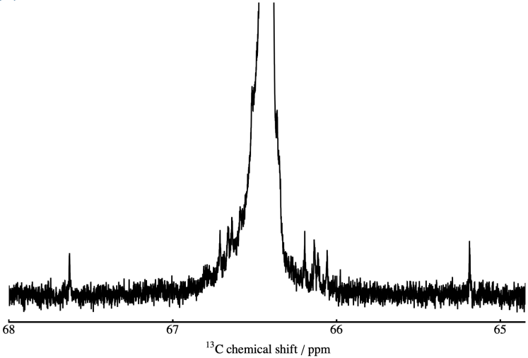
Figure 1: A portion surrounding the main doublet of the 700 MHz $90^{\circ}$ pulse-acquire spectrum, showing the weak transitions at 65.19 and 67.63 ppm.

2 Relaxation Superoperator

2.1 Derivation

A spin Hamiltonian for interaction $\Lambda$ may be written as a tensor product between a time-dependent spatial tensor and time-independent spin tensor. A convenient set of tensors to use are the irreducible spherical tensor operators, since these are eigenoperators of the Zeeman Hamiltonian commutation superoperator, leading to a simple expression in the corresponding interaction representation. For a rank-l interaction, we have, ¹

$$H^{\Lambda}_{l}(t)=c^{\Lambda}\sum_{m=-l}^{+l}A^{\Lambda*}_{lm}(t)X^{\Lambda}_{lm},$$ (1)

where $c^{\Lambda}$ is a real constant specific to interaction $\Lambda$. Being Hermitian, we may also write,

$$\begin{split}H^{\Lambda}_{l}(t)&=H^{\Lambda\dagger}_{l}\\ &=c^{\Lambda}\sum_{m=-l}^{+l}A^{\Lambda}_{lm}(t)X^{\Lambda\dagger}_{lm}.\end{split}$$ (2)

Useful relations for components $A_{lm}$ and $X_{lm}$ are,

$$A^{*}_{lm}=(-1)^{m}A_{l-m},$$ (3)

and,

$$X^{\dagger}_{lm}=(-1)^{m}X_{l-m}.$$ (4)

Then, using the eigenoperator relation,

$$\big{[}I_{z},X_{lm}\big{]}=mX_{lm},$$ (5)

the tensor components may be written in the interaction representation of the Zeeman interaction as,

$$\begin{split}\tilde{X}_{lm}(t)&=e^{i\hat{H}_{\mathrm{Z}}t}X_{lm}\\ &=X_{lm}e^{im\omega_{0}t},\end{split}$$ (6)

where $\hat{H}_{\mathrm{Z}}$ is the Zeeman Hamiltonian commutation superoperator, $\hat{H}_{\mathrm{Z}}=\big{[}H_{\mathrm{Z}},\cdots\big{]}=\omega_{0}\big{[}I_{\mathrm{z}},\cdots\big{]}$. In a Wangsness-Bloch-Redfield (WBR) formalism, the relaxation superoperator takes the form,

$$\hat{\Gamma}=-\frac{1}{2}\int^{+\infty}_{-\infty}d\tau\overline{\hat{\tilde{H}}_{\mathrm{fluc}}(t),\hat{\tilde{H}}_{\mathrm{fluc}}(t+\tau)}.$$ (7)

From here, we simplify the expression. First, we have the liberty of setting $t=0$ by assuming the noise in the system is stationary. This removes an exponential term in the interaction representation. Also, by neglecting the small dynamic frequency shifts, the correlation function has time-reversal symmetry and the integral may be taken from $-\infty$ to $0$ while introducing a factor of two. We now write,

$$\hat{\Gamma}=-\int^{0}_{-\infty}d\tau\overline{\hat{\tilde{H}}_{\mathrm{fluc}}(0)\hat{\tilde{H}}_{\mathrm{fluc}}(\tau)}.$$ (8)

$\hat{\Gamma}$ may be decomposed as a sum of auto- and cross-correlated relaxation superoperators. Simply,

$$\hat{\Gamma}=\sum_{\Lambda,\Lambda^{\prime}}\sum_{l,l^{\prime}}\hat{\Gamma}^{\Lambda\Lambda^{\prime}}_{ll^{\prime}},$$ (9)

and using eq. (1) while utilising (2), $\hat{\Gamma}^{\Lambda\Lambda^{\prime}}_{ll^{\prime}}$ takes the form,

$$\hat{\Gamma}^{\Lambda\Lambda^{\prime}}_{ll^{\prime}}=-c^{\Lambda}c^{\Lambda^{\prime}}\sum_{mm^{\prime}}J^{\Lambda\Lambda^{\prime}}_{ll^{\prime}mm^{\prime}}(\omega_{0})\Big{[}\hat{X}^{\Lambda}_{lm}\Big{]}^{L}\Big{[}\hat{X}^{\Lambda^{\prime}\dagger}_{l^{\prime}m^{\prime}}\Big{]}^{L},$$ (10)

where the spectral density function is given by,

$$J^{\Lambda\Lambda^{\prime}}_{ll^{\prime}mm^{\prime}}(\omega_{0})=\mathrm{Re}\int^{0}_{-\infty}d\tau\overline{\Big{[}A^{\Lambda*}_{lm}(0)\Big{]}^{L}\Big{[}A^{\Lambda^{\prime}}_{l^{\prime}m^{\prime}}(\tau)\Big{]}^{L}}e^{-im^{\prime}\omega_{0}|\tau|}.$$ (11)

Here, the square brackets with the superscript $L$ denote the laboratory frame. This is important since the spatial functions and spin tensors must be expressed in the same frame to legitimise the Hamiltonian they are associated with. However, the spatial functions are known in the molecule-fixed principal axis ($P$-) frame of the interaction in question, whereas the spin tensors are known in the space-fixed $L$-frame. Thus, we transform the spatial functions in the $L$-frame as a linear combination of functions in the diffusion ($D$-) frame using the properties of Wigner functions, before themselves being transformed as a linear combination of functions in the $P$-frame.

The relation to use is,

$$\Big{[}A_{lm}(t)\Big{]}^{L}=\sum_{n}\Big{[}A_{ln}\Big{]}^{D}D^{(l)}_{nm}(\Omega_{DL}(t)),$$ (12)

and the ensemble-averaged product in eq. (11) for the system becomes,

$$\begin{split}\overline{\Big{[}A^{\Lambda*}_{lm}(0)\Big{]}^{L}\Big{[}A^{\Lambda^{\prime}}_{l^{\prime}m^{\prime}}(\tau)\Big{]}^{L}}=\sum_{nn^{\prime}}&\overline{D^{(l)}_{mn}(\Omega_{LD}(0))D^{(l^{\prime})*}_{m^{\prime}n^{\prime}}(\Omega_{LD}(\tau))}\\ &\times\Big{[}A^{\Lambda*}_{ln}\Big{]}^{D}\Big{[}A^{\Lambda^{\prime}}_{l^{\prime}n^{\prime}}\Big{]}^{D},\end{split}$$ (13)

where the relation $D^{(l)}_{nm}(\Omega)=D^{(l)*}_{mn}(\Omega^{-1})$ is used, and $\Omega^{-1}_{DL}\equiv\Omega_{LD}$. The time-dependence of the spatial functions in the $L$-frame has been absorbed into the Wigner functions, since the $D$-frame is molecule-fixed. We then define the time-correlation function as that between the Wigner functions only, as,

$$\begin{split}G^{ll^{\prime}}_{mm^{\prime}nn^{\prime}}(\tau)&=\overline{D^{(l)}_{mn}(\Omega_{LD}(0))D^{(l^{\prime})*}_{m^{\prime}n^{\prime}}(\Omega_{LD}(\tau))}\\ &=\int\int d\Omega(0)d\Omega(\tau)D^{(l)}_{mn}(\Omega(0))D^{(l^{\prime})*}_{m^{\prime}n^{\prime}}(\Omega(\tau))\times P(\Omega(0))P(\Omega(\tau)|\Omega(0)),\end{split}$$ (14)

where $\Omega^{-1}_{DL}$ have been denoted simply by $\Omega$ in the second line for brevity, $P(\Omega(0))=1/(8\pi^{2})$ and is the probability that the molecule hosting the spin system will be at orientation $\Omega$ at time $t=0$, and $P(\Omega(\tau)|\Omega(0))$ is the conditional probability that the molecule will be at orientation $\Omega(\tau)$ at time $t^{\prime}=t+\tau=\tau$ given that it was at orientation $\Omega(0)$ at time $t=0$. From here, the notation and derivation is in similar vein of Huntress ^{2, 3}.

The time-derivative of the probability that the molecule will be at orientation $\Omega(\tau)$ at time $\tau$, in the limit of a rigid molecule reorienting in random steps of small angular displacement, is given by the Favro equation ⁴,

$$\frac{\partial}{\partial\tau}P(\Omega(\tau))=-H_{\mathrm{rot-diff}}P(\Omega(\tau)),$$ (15)

where $H_{\mathrm{rot-diff}}$ is the rotational-diffusion Hamiltonian, which may be written in the form,

$$H_{\mathrm{rot-diff}}=\mathbf{L}\bullet\mathbf{D}\bullet\mathbf{L}$$ (16)

where $\mathbf{L}$ and $\mathbf{D}$ are the quantum mechanical angular momentum operator and diffusion tensor, respectively. That is, the diffusion tensor describes the spatial aspect of the Hamiltonian in this case.

Favro shows that the solution to equation (15) is ⁴,

$$P(\Omega(\tau))=\int d\Omega(0)P(\Omega(0))P(\Omega(0)|\Omega(\tau)),$$ (17)

for which the conditional probability is,

$$P(\Omega(0)|\Omega(\tau))=\sum_{\nu}\psi^{*}_{\nu}(\Omega(0))\psi_{\nu}(\Omega(\tau))e^{-E_{\nu}\tau},$$ (18)

noindent where $\psi(\Omega)$ are eigenfunctions of $H_{\mathrm{rot-diff}}$ with the associated eigenvalue $E_{\nu}$. This solution is reliant on the boundary condition $P(\Omega(0)|\Omega(\tau\rightarrow 0))=\delta(\Omega(0),\Omega(\tau))$, where $\delta(\Omega(0),\Omega(\tau))$ is the Dirac delta function.

If eq. (16) is written in the $D$-frame, it takes the form $H_{\mathrm{rot-diff}}=\sum_{i}D_{i}L^{2}_{i}$ in which $i\in\{x,y,z\}$ and $L_{i}$ have become the Cartesian angular momentum operators. This takes the form of the rigid-rotor Hamiltonian when considering the substitution $D_{i}\rightarrow\hbar^{2}/2I_{i}$, where $I_{i}$ is the moment of inertia about principal axis $i$. Thus, (18) may be expanded in asymmetric-rotor eigenfunctions,

$$P(\Omega(\tau)|\Omega(0))=\sum_{\nu,J,M}\psi^{J*}_{\nu,M}(0)\psi^{J}_{\nu,M}(\tau)e^{-E^{J}_{\nu}\tau},$$ (19)

where,

$$\psi^{J}_{\nu,M}(t)=\sum_{K}a^{J}_{\nu,K}\phi^{J}_{K,M}$$ (20)

and $\phi^{J}_{K,M}$ are symmetric-rotor eigenfunctions which may be expressed in terms of Wigner functions and take the form,

$$\phi^{J}_{K,M}=(-1)^{M-K}\sqrt{\frac{2J+1}{8\pi^{2}}}D^{(J)}_{-M-K}(\Omega).$$ (21)

We then have all we need to obtain the time-correlation function and subsequently the spectral density function and relaxation superoperator. Inserting these eigenfunctions and probabilities into (33) and setting $\Omega\equiv\Omega_{LD}$ in (21),

$$\begin{split}G^{ll^{\prime}}_{mm^{\prime}nn^{\prime}}(\tau)=&\frac{1}{8\pi^{2}}\sum_{\nu,J,M}(2J+1)e^{-E^{J}_{\nu}\tau}\\ &\times\int\int d\Omega_{LD}(0)d\Omega_{LD}(\tau)D^{(l)}_{mn}(\Omega_{LD}(0))D^{(l^{\prime})*}_{m^{\prime}n^{\prime}}(\Omega_{LD}(\tau))\\ &\times\bigg{\{}\sum_{K}a^{J*}_{\nu,K}(-1)^{M-K}D^{(J)*}_{-M-K}(\Omega_{LD}(0))\bigg{\}}\\ &\times\bigg{\{}\sum_{K^{\prime}}a^{J}_{\nu,K^{\prime}}(-1)^{M-K^{\prime}}D^{(J)}_{-M-K^{\prime}}(\Omega_{LD}(\tau))\bigg{\}},\end{split}$$ (22)

and rearranging the expression, while using the orthogonality relation,

$$\int d\Omega D^{j}_{pq}(\Omega)D^{j^{\prime}}_{p^{\prime}q^{\prime}}(\Omega)=\frac{8\pi^{2}}{2j+1}\delta_{jj^{\prime}}\delta_{pp^{\prime}}\delta_{qq^{\prime}},$$ (23)

the time correlation function simplifies to,

$$\begin{split}G^{l}_{mnn^{\prime}}(\tau)&=\delta_{ll^{\prime}}\delta_{mm^{\prime}}G^{ll^{\prime}}_{mm^{\prime}nn^{\prime}}(\tau)\\ &=\frac{(-1)^{n+n^{\prime}}}{2l+1}\sum_{\nu}a^{l*}_{\nu,n}a^{l}_{\nu,-n^{\prime}}e^{-E^{l}_{\nu}\tau},\end{split}$$ (24)

where $l=l^{\prime}=J$, $m=m^{\prime}=-M$, $n=-K$ and $n^{\prime}=-K^{\prime}$.

From this, the spectral density becomes,

$$\begin{split}J^{\Lambda\Lambda^{\prime}}_{lm}(\omega_{0})&=\delta_{ll^{\prime}}\delta_{mm^{\prime}}J^{\Lambda\Lambda^{\prime}}_{ll^{\prime}mm^{\prime}}(\omega_{0})\\ &=\mathrm{Re}\int_{-\infty}^{0}d\tau\overline{\Big{[}A^{\Lambda*}_{lm}(0)\Big{]}^{L}\Big{[}A^{\Lambda^{\prime}}_{lm}(\tau)\Big{]}^{L}}e^{-im\omega_{0}|\tau|}\\ &\begin{split}=\sum_{nn^{\prime}}\frac{(-1)^{n+n^{\prime}}}{2l+1}\sum_{\nu}&a^{l}_{\nu,n}a^{l}_{\nu,-n^{\prime}}\Big{[}A^{\Lambda*}_{ln}\Big{]}^{D}\Big{[}A^{\Lambda^{\prime}}_{ln^{\prime}}\Big{]}^{D}\\ &\times\mathrm{Re}\int_{-\infty}^{0}d\tau e^{-E^{l}_{\nu}\tau}e^{-im\omega_{0}|\tau|}.\end{split}\end{split}$$ (25)

Performing the integral and inserting back into the relaxation superoperator, we have,

$$\begin{split}\hat{\Gamma}^{\Lambda\Lambda^{\prime}}_{l}&=\delta_{ll^{\prime}}\hat{\Gamma}^{\Lambda\Lambda^{\prime}}_{ll^{\prime}}\\ &=-c^{\Lambda}c^{\Lambda^{\prime}}\sum_{m}J^{\Lambda\Lambda^{\prime}}_{lm}(\omega_{0})\Big{[}\hat{X}^{\Lambda}_{lm}\Big{]}^{L}\Big{[}\hat{X}^{\Lambda^{\prime}\dagger}_{lm}\Big{]}^{L},\end{split}$$ (26)

with,

$$\begin{split}J^{\Lambda\Lambda^{\prime}}_{lm}(\omega_{0})=\sum_{nn^{\prime}}&\frac{(-1)^{n+n^{\prime}}}{2l+1}\Big{[}A^{\Lambda*}_{ln}\Big{]}^{D}\Big{[}A^{\Lambda^{\prime}}_{ln^{\prime}}\Big{]}^{D}\\ &\times\sum_{\nu}a^{l}_{\nu,n}a^{l}_{\nu,-n^{\prime}}\frac{E^{l}_{\nu}}{E^{(l)2}_{\nu}+m^{2}\omega^{2}_{0}}.\end{split}$$ (27)

This is the general case of an asymmetric-top molecule. To derive the case for a symmetric rotor with the $P$- and $D$-frames coincident (as in our model), we refer back to eq. (16), where we may write it in the $D$-frame as,

$$H_{\mathrm{rot-diff}}=D_{\perp}\left(L^{2}_{x}+L^{2}_{y}\right)+D_{\parallel}L^{2}_{z}$$ (28)

where $D_{\perp}$ and $D_{\parallel}$ are rotational diffusion constants associated with axes perpendicular and parallel, respectively, with the spin chain.

Eq. (28) is of the same form as the rigid-rotor Hamiltonian for a symmetric-top. As such, the eigenfunctions and eigenvalues in eq. (18) are those of a quantum mechanical rigid-rotor ^{5, 6}:

$$\psi_{\nu}(t)\xrightarrow[]{}\phi^{J}_{K,M}(t)\equiv(-1)^{M-K}\sqrt{\frac{2J+1}{8\pi^{2}}}D^{(J)}_{-M-K}(\Omega(t))$$ (29)

$$E_{\nu}\xrightarrow[]{}E^{J}_{K}\equiv D_{\perp}J(J+1)+K^{2}(D_{\parallel}-D_{\perp}).$$ (30)

For our specific system, $J\equiv l=2$ and $K=0$. To see this, note that the only non-zero component for the dipole-dipole (DD) interaction is $\left[A^{\mathrm{DD}}_{20}\right]^{P}=\sqrt{6}$ in the $P$-frame. The $z$-principal axis is defined as a vector connecting the two nuclei in question. We then assume this is coincident with the $z$-axis in the $D$-frame, with the $x$- and $y$-axes arbitrary. Writing, $D^{(l)}_{mn}(\alpha,\beta,\gamma)=e^{-im\alpha}d^{(l)}_{mn}(\beta)e^{-in\gamma}$ and assuming coincidence of the $P$- and $D$-frames (i.e. $\{\alpha,\beta,\gamma\}=\{0,0,0\}$), eq. (12) may be written,

$$\begin{split}\Big{[}A^{\mathrm{DD}}_{20}\Big{]}^{P}&=\sum_{n}\Big{[}A^{\mathrm{DD}}_{2n}\Big{]}^{D}d^{(2)}_{n0}(\beta=0)\\ &=\Big{[}A^{\mathrm{DD}}_{20}\Big{]}^{D},\end{split}$$ (31)

where $d^{(2)}_{00}(\beta)=\frac{3\mathrm{cos}^{2}\beta-1}{2}$ is the only non-vanishing reduced Wigner function, and equates to unity for $\beta=0$.

In general, the CSA $P$-frame will not be coincident with the DD $P$-frame. To simplify analytical expressions in the main text, however, they are assumed to be so for our system. Also, assuming cylindrical symmetry of the rigid-rod, the biaxiality parameters may be approximated as 0. Then the same relation holds for the CSA interaction; i.e. the only non-vanishing component of the spatial tensor is,

$$\Big{[}A^{\mathrm{CSA}}_{20}\Big{]}^{P}=\Big{[}A^{\mathrm{CSA}}_{20}\Big{]}^{D}.$$ (32)

Since $n=K$, the only non-vanishing term in the correlation function is then $E^{(2)}_{0}=6D_{\perp}$, and related to the rotational correlation time $\tau_{\perp}\equiv\big{(}6D_{\perp}\big{)}^{-1}$. We then see that rotational motion about the principal axis of inertia parallel to the rod does not modulate the interactions responsible for relaxation, and this is a consequence of the coincidence of the $P$- and $D$-frames, as well as the assumption that the molecule tumbles rigidly. The secularised time-correlation function for our system becomes,

$$G^{ll^{\prime}}_{mm^{\prime}nn^{\prime}}(\tau)=\delta_{ll^{\prime}}\delta_{mm^{\prime}}\frac{(-1)^{n+n^{\prime}}}{2l+1}e^{-\tau/\tau_{\perp}}.$$ (33)

The $(-1)$-QC subspace of the Liouvillian is given below. This shows that the off-diagonal elements are orders of magnitude smaller than the diagonal elements, and we, therefore, use the $\mathbb{B}_{Q}$ basis and regard relaxation as a small perturbation when determining peak position. Also, since the mixing angle $\theta=\mathrm{arctan}\left(\omega_{\Delta}/\omega_{J}\right)=-0.075$, the $\mathbb{B}_{\mathrm{ST}}$ is used to simplify the $\lambda_{\pm}$ expressions in the main text. The $(-1)$-QC subspace of the Liouvillian is,

$$\hat{\mathcal{L}}_{4\times 4}=\bordermatrix{~{}&\big{|}|S^{\prime}_{0}\rangle\langle T^{\prime}_{+1}|\big{)}&\big{|}|T^{\prime}_{-1}\rangle\langle S^{\prime}_{0}|\big{)}&\big{|}|T^{\prime}_{0}\rangle\langle T^{\prime}_{+1}|\big{)}&\big{|}|T^{\prime}_{-1}\rangle\langle T^{\prime}_{0}|\big{)}\cr\big{|}|S^{\prime}_{0}\rangle\langle T^{\prime}_{+1}|\big{)}&-0.0852+1339.86i&13.43\times 10^{-5}&-3.16\times 10^{-3}&3.47\times 10^{-3}\cr\big{|}|T^{\prime}_{-1}\rangle\langle S^{\prime}_{0}|\big{)}&13.43\times 10^{-5}&-0.180-1339.86i&3.65\times 10^{-3}&-5.78\times 10^{-3}\cr\big{|}|T^{\prime}_{0}\rangle\langle T^{\prime}_{+1}|\big{)}&-3.16\times 10^{-3}&3.65\times 10^{-3}&-0.168+5.68i&94.16\times 10^{-3}\cr\big{|}|T^{\prime}_{-1}\rangle\langle T^{\prime}_{0}|\big{)}&3.47\times 10^{-3}&-5.77\times 10^{-3}&94.16\times 10^{-3}&-0.338-5.68i}\ \mathrm{s}^{-1}.$$ (34)

The real part is plotted is derived from the relaxation superoperator alone, and is plotted in figure 2.

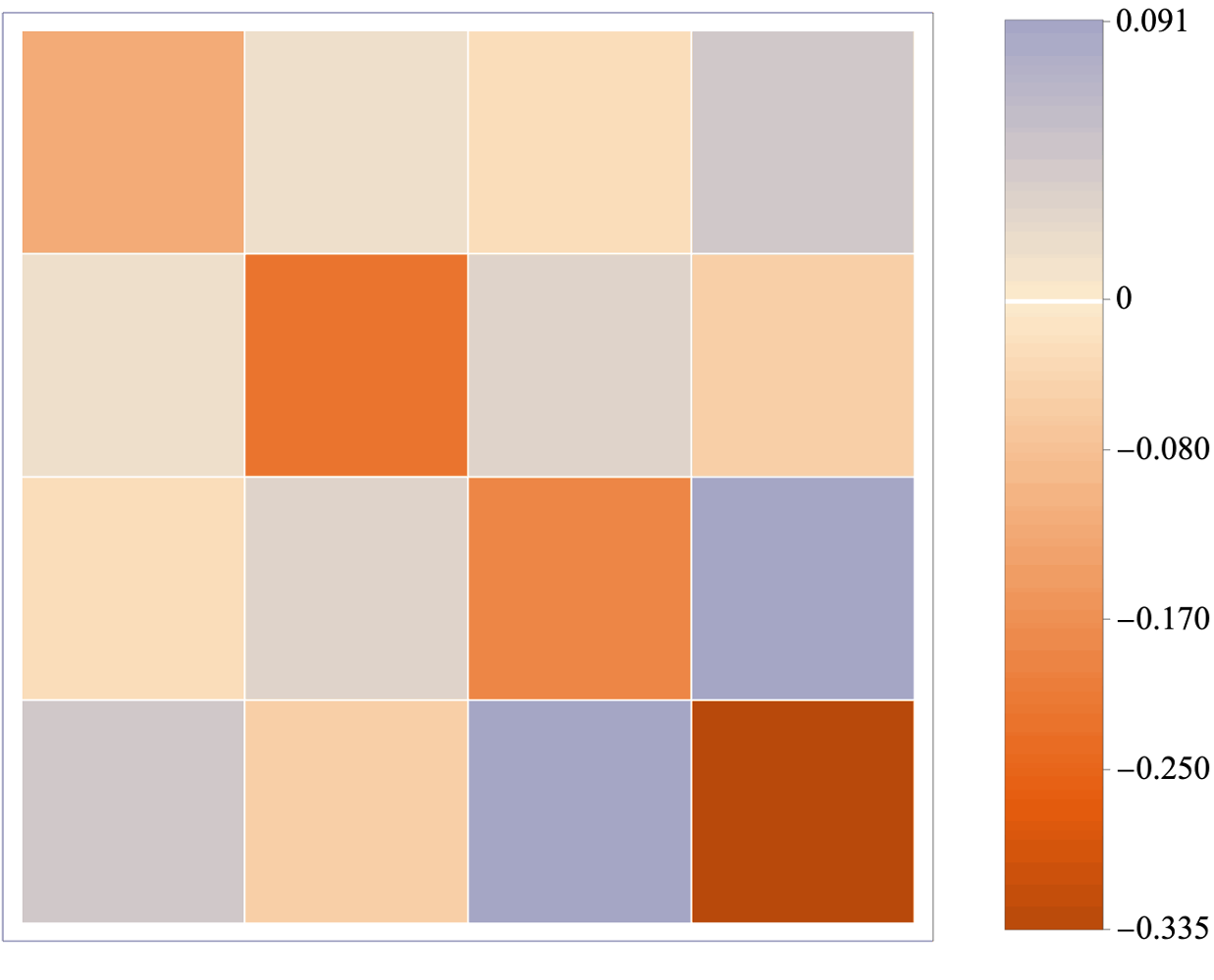
Figure 2: The $\ (-1)$-QC block of the real part of the Liouvillian in the $\mathbb{B}_{Q}$ basis.

The computed magnetic shielding tensors are given in their respective $P$-frames by:

$$\mathbf{\sigma}_{1}=\begin{pmatrix}258.73&0&0\\ 0&41.59&0\\ 0&0&38.65\end{pmatrix}\mathrm{ppm},$$ (35)

and,

$$\mathbf{\sigma}_{2}=\begin{pmatrix}258.64&0&0\\ 0&42.25&0\\ 0&0&38.90\end{pmatrix}\mathrm{ppm}.$$ (36)

These are transformed to the chemical shift tensor $\delta$ by the relation,

$$\mathbf{\delta}=\mathbb{I}\sigma_{\mathrm{TMS}}^{\mathrm{iso}}-\mathbb{\sigma},$$ (37)

where $\mathbb{I}$ is the three-dimensional identity matrix, and $\sigma_{\mathrm{TMS}}^{\mathrm{iso}}$ is the isotropic component of the magnetic shielding tensor of tetramethylsilane, acting as a reference.

The shielding tensors (35) and (36) are transformed to their principal axis frames by diagonalisation. Then, the Haeberlen convention ⁷ is used to define the anisotropy and biaxiality parameters, respectively, as,

$$\delta^{\mathrm{CSA}}=\delta^{\mathrm{P}}_{zz}-\delta^{\mathrm{iso}}$$ (38)

and,

$$\eta=\frac{\delta^{\mathrm{P}}_{xx}-\delta^{\mathrm{P}}_{yy}}{\delta^{\mathrm{CSA}}},$$ (39)

with tensor components defined by,

$$|\delta^{\mathrm{P}}_{zz}-\delta^{\mathrm{iso}}|\geq|\delta^{\mathrm{P}}_{xx}-\delta^{\mathrm{iso}}|\geq|\delta^{\mathrm{P}}_{yy}-\delta^{\mathrm{iso}}|.$$ (40)

2.2 Estimation of $\tau_{\perp}$

The correlation time was estimated using the experimental $T_{1}=2.24\ \mathrm{s}$ value and the relation,

$$T^{-1}_{1}\simeq-\frac{\big{(}I_{z}\big{|}\hat{\Gamma}\big{|}I_{z}\big{)}}{\big{(}I_{z}\big{|}I_{z}\big{)}},$$ (41)

and solving for $\tau_{\perp}$.

3 Synthesis of Target Triyne 5

3.1 Synthesis of intermediate 2

To a stirred suspension of CuCl (41.6 mg, 0.42 mmol) in acetone (4 mL) was added tetramethylethylenediamine (TMEDA, 22.0 µL, 0.14 mmol), and the mixture was stirred for 30 minutes. Then, a mixture of 1-ethynyl-4-methoxybenzene 1 (264.3 mg, 2.0 mmol) and (trimethylsilyl)acetylene-${}^{13}\mathrm{C}_{2}$ (288 µL, 2.0 mmol) in acetone (4 mL) was added slowly and bubbled with $\mathrm{O}_{2}$ for 5 min. The reaction mixture was stirred for 2 h at room temperature, and then passed through a pad of silica gel. Then, the filtrate was concentrated under reduced pressure and the residue was purified by column chromatography using $\mathrm{Et}_{2}\mathrm{O/hexane}$ (1:15) as eluent to afford compound 2 (332 mg, 72%) as a colorless oil. ${}^{1}\mathrm{H}$ NMR (400 MHz, $\mathrm{CDCl}_{3}$): $\delta$ 0.24 (dd, $J=2.5$, 0.6 Hz, 9 H), 3.82 (s, 3 H), 6.84 (d, $J=9.4$ Hz, 2 H), 7.44 (d, $J=9.4$ Hz, 2 H). ${}^{13}\mathrm{C}\{^{1}\mathrm{H}\}$ NMR (101 MHz, $\mathrm{CDCl}_{3}$): $\delta$ 87.8 (d, $J=144.5$ Hz, 1 C), 90.1 (d, $J=144.5$ Hz, 1 C) (only ${}^{13}\mathrm{C}$-enriched signals are shown). LRMS (ES+) $m/z$ 231.1 (100%, [M + H]⁺).

3.2 Synthesis of intermediate 3

A mixture of 2 (320 mg, 1.39 mmol), $\mathrm{K}_{2}\mathrm{CO}_{3}$ (384 mg, 2.78 mmol), MeOH (5 mL) and THF (5 mL) was stirred at room temperature for 1 h. Then, the reaction mixture was extracted with ethyl acetate and washed with brine. Evaporation of the solvent afforded diacetylene 3 (215 mg, 98%) as a colorless solid, which was used for the next step without further purification. ${}^{1}\mathrm{H}$ NMR (400 MHz, $\mathrm{CDCl}_{3}$): $\delta$ 2.46 (dd, $J=232.8$, 77.8 Hz, 1H), 3.83 (s, 3H), 6.85 (d, $J=8.9$ Hz, 1 H), 7.47 (d, $J=8.93$ Hz, 2 H). ${}^{13}\mathrm{C}\{^{1}\mathrm{H}\}$ NMR (101 MHz, $\mathrm{CDCl}_{3}$): $\delta$ 68.03 (d, $J=192.20$ Hz, 1 C), 71.04 (d, $J=191.47$ Hz, 1 C) (only ${}^{13}\mathrm{C}$-enriched signals are shown). LRMS (ES+) $m/z$ 159.1 (100%, [M + H]⁺).

3.3 Synthesis of triyne I

To a solution of diacetylene 3 (197 mg, 1.26 mmol) in toluene (2.5 mL) at 0 °C were added CuCl (18.8 mg, 0.19 mmol), $\mathrm{NH}_{2}\mathrm{OH}\bullet\mathrm{HCl}$ (26.3 mg, 0.38 mmol) and $n$-$\mathrm{BuNH}_{2}$ (188 µL, 1.9 mmol) in order. Alkynyl bromide 4 (304 mg, 1.26 mmol) was diluted with 2.5 mL toluene and was added dropwise to the mixture. The reaction mixture was allowed to warm to room temperature and stir for 18 h. The reaction was quenched with $\mathrm{H}_{2}\mathrm{O}$ and extracted with ether. The organic layer was washed with $\mathrm{H}_{2}\mathrm{O}$, brine and dried over $\mathrm{MgSO}_{4}$. The solvent was evaporated, and the residue was purified by column chromatography using dichloromethane/hexane (1:2) as eluent to afford triyne I (263 mg, 66%) as a colorless solid. ${}^{1}\mathrm{H}$ NMR (400 MHz, $\mathrm{CDCl}_{3}$): $\delta$ 3.48 (s, 3 H), 3.84 (s, 3 H), 5.20 (s, 2 H), 6.86 (d, $J=8.0$ Hz, 2 H) 7.00 (d, $J=8.0$ Hz, 2 H), 7.50 (d, $J=8.9$ Hz, 2 H), 7.49 (d, $J=8.9$ Hz, 2 H). ${}^{13}\mathrm{C}\{^{1}\mathrm{H}\}$ NMR (101 MHz, $\mathrm{CDCl}_{3}$): $\delta$ 66.41 (d, $J=217.0$ Hz, 1 C), 66.39 (d, $J=217.0$ Hz, 1 C) (only ${}^{13}\mathrm{C}$-enriched signals are shown). LRMS (ES+) $m/z$ 317.1 (100%, [M + H]⁺).

References

Smith, Palke, and Gerig 1992aS. A. Smith, W. E. Palke, and J. T. Gerig, “The Hamiltonians of
NMR. part I,” Concepts Magn. Reson. 4, 107–144 (1992a).
Huntress 1968W. T. Huntress, “Effects of
Anisotropic Molecular Rotational Diffusion on Nuclear Magnetic
Relaxation in Liquids,” J. Chem. Phys. 48, 3524–3533 (1968).
Huntress 1970W. T. Huntress, “The Study
of Anisotropic Rotation of Molecules in Liquids by NMR
Quadrupolar Relaxation,” in Advances in Magnetic and Optical Resonance, Vol. 4, edited by J. S. Waugh (Academic Press, 1970) pp. 1–37.
Favro 1960L. D. Favro, “Theory of the
Rotational Brownian Motion of a Free Rigid Body,” Phys. Rev. 119, 53–62 (1960).
Zare 1988R. N. Zare, Angular Momentum:
Understanding Spatial Aspects in Chemistry and Physics, The George
Fisher Baker Non-Resident Lectureship in Chemistry at Cornell
University (Wiley, New
York, 1988).
Wang 1973C. Wang, “Anisotropic-rotational diffusion model calculation of T1 due to
spin-rotation interaction in liquids,” Journal of Magnetic Resonance (1969) 9, 75–83 (1973).
Haeberlen 1976U. Haeberlen, High Resolution
NMR in Solids: Selective Averaging, Advances in
Magnetic Resonance : Supplement No. 1 (Academic Press, New York, 1976).