Co-scheduling Ensembles of In Situ Workflows

Abstract

Molecular dynamics (MD) simulations are widely used to study large-scale molecular systems. HPC systems are ideal platforms to run these studies, however, reaching the necessary simulation timescale to detect rare processes is challenging, even with modern supercomputers. To overcome the timescale limitation, the simulation of a long MD trajectory is replaced by multiple short-range simulations that are executed simultaneously in an ensemble of simulations. Analyses are usually co-scheduled with these simulations to efficiently process large volumes of data generated by the simulations at runtime, thanks to in situ techniques. Executing a workflow ensemble of simulations and their in situ analyses requires efficient co-scheduling strategies and sophisticated management of computational resources so that they are not slowing down each other. In this paper, we propose an efficient method to co-schedule simulations and in situ analyses such that the makespan of the workflow ensemble is minimized. We present a novel approach to allocate resources for a workflow ensemble under resource constraints by using a theoretical framework modeling the workflow ensemble’s execution. We evaluate the proposed approach using an accurate simulator based on the WRENCH simulation framework on various workflow ensemble configurations. Results demonstrate the significance of co-scheduling simulations and in situ analyses that couple data together to benefit from data locality, in which inefficient scheduling decisions can lead up to a factor 30 slowdown in makespan.

I Introduction

Molecular dynamics (MD) is one of the scientific simulations that benefit most from ever-increasing computational capabilities offered by modern high-performance computing (HPC) platforms. MD simulations serve as a productive method to observe relevant processes of a molecular system at atomic resolution. MD simulations discover the motion of the system through computing atomic positions that evolve over time. MD simulations regularly generate large amount of data that needs to be stored efficiently to disks. However, I/O capabilities have not evolved as fast as compute capabilities in contemporary HPC infrastructures, which causes an important performance bottleneck at scale [1] due to large amount of data generated by the simulations that cannot be stored efficiently to disks. Consequently, the community has developed different approaches to overcome the I/O bottleneck—in this work, we focus on a particular one called in situ. The in situ paradigm shifts the data processing phase from traditional post-processing to iterative processing following a producer-consumer approach. Basically, instead of storing data produced by simulations on disks, simulations send data periodically using faster memories (e.g., DRAM, SSD) to in situ analysis jobs that run concurrently to the simulations. Performing analyses in situ does not only help to obtain on-the-fly insights into the molecular system at runtime, but it also reduces the burden on the file system.

Interesting molecular events require observing at a long enough simulation timescale, which is compute-intensive for simulating large-scale molecular systems. To overcome this timescale problem, a family of enhanced-sampling methods utilizes multiple short-range simulations running within ensembles to efficiently explore different regions of the conformational space. Ensemble-based computational methods [2, 3, 4, 5] are gaining popularity in many scientific domains using computational simulations, where computations are executed as jobs into a workflow ensemble. A workflow ensemble [6] is usually composed of a number of inter-related workflows, for example identical workflows of simulation-analysis pipeline with different input parameters exploring the solutions space. We consider the execution of ensembles of in situ workflows in which concurrent jobs, i.e. simulations and analyses, are tightly coupled using in situ processing, thereby usually co-scheduled together to efficiently process data at runtime. However, sustaining complex co-scheduling for massive workflow ensembles of concurrent applications will require sophisticated orchestration tailored for the management of workflow ensembles [7, 8].

In this paper, we aim to guide the above emerging orchestration runtime. The key challenge when orchestrating the workflow ensembles at scale is to efficiently schedule the simulations and in situ analyses as they continuously exchange data. The intersection of workflow ensembles and in situ is particularly challenging as in situ itself has intricate, complex communication patterns, which is further convoluted by the number of concurrent executions at scale. Intuitively, co-scheduling the analyses with their associated simulation on the same computing resources improves data locality, but required resources may not be consistently available. Thus, upon resource constraint, how do we co-schedule workflow ensembles on a HPC machine? A key distinguishing factor is to efficiently generate large ensembles to optimize scientific discoveries. Another major challenge is to determine resource requirements such that the resulting performance of executing them together in the workflow ensemble is maximized. Therefore, we design efficient co-scheduling strategies and resource assignments for the workflow ensemble of simulations and in situ analyses. Our contributions are as follows:

• We develop a mathematical model that characterizes iterative execution and data coupling behavior of simulations and in situ analyses in a workflow ensemble.

• We use this model to derive optimal co-scheduling strategies and compute resource allocations for the simulations and in situ analyses in the workflow ensemble under constraints of the available computing resources.

• We evaluate our proposed scheduling solutions using an accurate simulator by studying different co-scheduling scenarios on various configurations of the workflow ensembles.

II Related Work

Designing scheduling algorithms for in situ workflows such that available resources are efficiently utilized is challenging as optimizing individual workflow components does not ensure that the end-to-end performance of the workflow is optimal. The larger the number of components the workflow has, the larger the multi-parametric space needed to explore. Specifically, workflow ensembles consist of many simulations and in situ analyses running concurrently, thus the combination of their data coupling behaviors significantly increases the complexity of the scheduling decisions. Few efforts have been attempted to solve this problem on a single in situ workflow. Malakar et al. formulated the in situ coupling between the simulation and the analysis as a mixed-integer linear programming problem [9] and derived the frequency to schedule the analysis executed in situ on different set of nodes. Aupy et al. proposed a greedy algorithm [10] to schedule a set of in situ analyses on available resources with memory constraints. Taufer et al. introduced a 2-step model [11] to predict the frequency of frames to be analyzed in situ such that computing resources are not underutilized while the simulation is not slowed down by the analysis. Our proposed approach for scheduling is not restricted to a single in situ coupling.

Co-scheduling strategies have been recently proposed to deliver better resource utilization and increasing overall application throughput [12, 13, 14]. However, only few works incorporated co-scheduling into the in situ workflows, where components (simulations and analyses) in the workflow are tightly coupled together. Sewell et al. proposed a thorough performance study [15] for co-scheduling in situ components that leverages memory system for data staging with low latencies. Aupy et al. introduced an optimization-based approach [16] to determine the optimal fraction of caches and cores allocated to in situ tasks. Due to the lack of capability to submit a batch of concurrent applications with conventional scheduler, co-scheduling was not fully-supported for the workflow ensembles at production scale. To overcome this limitation, Flux [7] was designed as a hierarchical resource manager to meet the needs of co-scheduling large-scale ensemble of various simulations and in situ analyses. To the best of our knowledge, this paper is the first effort that addresses co-scheduling problem for in situ workflows at ensemble level.

III Model

The goal of this paper is to study the scheduling of complex ensembles of in situ workflows [17] on parallel machines, where every workflow within an ensemble has several concurrent jobs coupled together using in situ processing, either be a simulation or an analysis. Unfortunately, one might not have enough compute nodes to run concurrently all simulations and analyses and, will have to make scheduling choices: (i) which simulation and analysis should run together on the same resources and (ii) how much resources should be allocated to each.

Our approach. The core of this work is to propose a powerful but versatile model to express complex data dependencies between simulations and in situ analyses in a workflow ensemble, and based on that design appropriate scheduling strategies. The chosen approach is to model the scheduling problem under simplified conditions where we make several assumptions to reduce the large space of exploration in an ensemble of in situ workflows. Then, we demonstrate that solutions designed for the simplified world, also perform well in using realistic settings.

III-A Couplings

A simulation $S_{i}$ represents a job in an ensemble that simulates a state of interest in the molecular system. An analysis, denoted as $A_{j}$, represents a computational kernel that is suitable to analyze in situ data produced by a simulation, e.g. transforming high-dimensional molecular structures to eigenvalue metadata [18]. Regularly, the output resulted by in situ analyses are later post-processed, e.g. synthesized to infer conformational changes of the molecular system in a post-hoc analysis. However, in the scope of this paper, we focus on the part of the simulation-analysis pipeline where they are executed simultaneously in an ensemble as it is more challenging to manage. We denote the set of simulations and analyses in an ensemble as $S$ and $A$ respectively. In this work, each workflow of an ensemble is composed of one simulation and at least one analysis. The analyses are executed in parallel with the simulation and periodically processed simulation data generated after each simulation steps in an iterative fashion. This essence of in situ processing expresses the important notion of coupling.

Coupling indicates which simulation and analyses have a data dependency, i.e. data produced by the simulation is analyzed by the corresponding analyses. Scientists usually decides beforehand which analyses have to process the data from a given simulation, we call this mapping a coupling (see Figure 1). Therefore, couplings are decided beforehand as an input of the problem. More formally, a coupling $p:S\rightarrow A$ defines which analyses in $A$ are coupled with which simulation in $S$, then for every $S_{i}\in S$, let $p(S_{i})$ be the set of analyses that couple data with the simulation $S_{i}$. For example, in Figure 1, we have $p(S_{1})=\{A_{1},A_{3}\}$. Now that we have defined the notion of couplings, we need to define different notions around co-scheduling.

III-B Co-scheduling

The notion of co-scheduling is at the core of this work, co-scheduling is defined as running multiple applications concurrently on the same set of compute nodes, each application using a fraction of the number of cores per node. We assume the total number of cores of each application is distributed evenly among the compute nodes the application is co-scheduled on, which is similar to the manner of distributing resources in emerging schedulers, e.g. Flux [7], for co-scheduling concurrent jobs of a massive ensemble in next-generation computers. In this paper, we distinguish two scenarios in which we map the simulations and analyses to computational resources:

• Co-scheduling: $S_{i}$ and $A_{j}$ run on the same compute nodes and thus have access to the shared memory;

• In transit: $S_{i}$ and $A_{j}$ run on two different set of nodes and sending data from $S_{i}$ to $A_{j}$ involves network communications.

In an attempt to avoid performance degradation in co-scheduling, in this work, we consider that simulations, which are compute-intensive, are not co-scheduled together [19]. Now we need to define several other important terms related to co-scheduling.

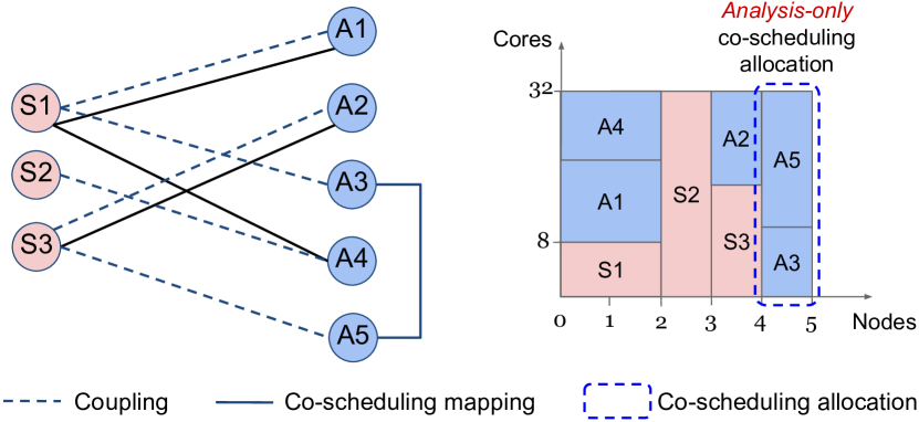
Figure 1: Illustration of co-scheduling and coupling notions.

Co-scheduling mapping. A co-scheduling mapping $m$ defines how $S$ and $A$ are co-scheduled together. For a given mapping $m$, we denote by $m(S_{i})$ the set of analyses co-scheduled with $S_{i}$. For example, with the mapping illustrated in Figure 1, $m(S_{1})=\{A_{1},A_{3}\}$ and $m(S_{3})=\{A_{2}\}$.

Assumption 1.

In this model, we ignore co-scheduling interference, such as cache sharing, that could degrade the performance when multiple applications share resources [19].

Co-scheduling allocation. A co-scheduling allocation represents a set of applications which are co-scheduled together (i.e., share computing resources). Let $\langle\{S_{i},A_{j}\}\rangle$ denote a co-scheduling allocation where simulation $S_{i}$ is co-scheduled with analysis $A_{j}$. Recall that, we have at most one simulation per allocation, but we can have multiple analyses. Formally, for a given co-scheduling mapping $m$, a simulation $S_{i}$ and analyses $m(S_{i})$ that are co-scheduled with $S_{i}$, the corresponding co-scheduling allocation is denoted by $\langle S_{i}\cup m(S_{i})\rangle$. However, not all analyses are required to be co-scheduled with a simulation, there exists co-scheduling allocations in which only analyses are co-scheduled together, called analysis-only co-scheduling allocations. For example, in Figure 1, $\langle\{A_{3},A_{5}\}\rangle$ is an analysis-only co-scheduling allocation. A co-scheduling allocation also determines the amount of computer resources assigned for each co-scheduled application. Let $n_{x}$ denote the number of nodes assigned to application $x$. For instance, if $S_{i}$ and $A_{j}$ are co-scheduled on the same co-scheduling allocation, then $n_{S_{i}}=n_{A_{j}}$. Let $c_{x}$ be the number of cores per node assigned to $x$. As each co-scheduled application takes a portion of cores in the total of $C$ cores a node has, then for every co-scheduling allocation $\langle X\rangle$, we have $\sum_{x\in X}c_{x}\leq C$ . In Figure 1, since $A_{1}$ and $A_{4}$ are co-scheduled with $S_{1}$ on a co-scheduling allocation spreading in 2 compute nodes, then $n_{S_{1}}=n_{A_{1}}=n_{A_{4}}=2$. And since $c_{S_{1}}=8$, then $S_{1}$ occupies 8 cores each node, so 16 cores in total.

III-C Execution platform

We consider a traditional parallel computing platform with $N$ identical compute nodes, each node has $C$ identical cores, a shared memory of size $M$ and a bandwidth of $B$ per node. In addition, we consider that the interconnect network between nodes is a fully-connected topology, hence the communication time is the same for any pairs of nodes.

III-D Application model

Because of the in situ execution, simulations and analyses are executed iteratively, in which iterations exhibit consistent behavior [20]. Specifically, the simulation executes certain compute-intensive tasks each iteration and then generates output data. The analysis, in every iteration, subscribes the data produced by the simulation and performs several specific computations. Since the complexity of computation and the amount of data are identical across iterations, the time to execute one iteration is approximately the same across iterations. Based on this reasoning and, by assuming the simulations and analyses have the same number of iterations ($n_{steps}$), we simply consider the execution time of a single iteration as the entire execution time can be derived from multiplying the time taken by a single iteration by $n_{steps}$ [20].

Computation model. Let us now denote by $t(x)$ the time to execute one iteration of the iterative application $x$ ($x$ can either be a simulation or an analysis). For readability, we pay particular attention to the class of perfectly parallel applications, even though the approach can be generalized to other models, such as Amdahl’s Law [21].

Assumption 2.

Every simulation and analysis follow a perfectly parallel speedup model [22].

In other words, a job $x$ that runs in time $t_{x}(1)$ on one core will run in time $t_{x}(1)/c$ when using $c$ cores. Thus, we can express the time to execute one iteration of the simulation as follows

$$t(S_{i})=\frac{t_{S_{i}}(1)}{n_{S_{i}}c_{S_{i}}},$$ (1)

where $S_{i}$ is running on $n_{S_{i}}$ compute nodes with $c_{S_{i}}$ cores each node.

Communication model. In in situ processing, data is usually stored on node-local storage [23] or local memory [24] to reduce the overhead associated with data movement. In this work, we process data residing in memory to allow near real-time data analysis. Data communications are modeled as follows: (i) $S_{i}$ writes its results into local memory of the nodes it runs on, and (ii) each analysis coupled with $S_{i}$ reads from that memory the data it needs whether locally or remotely depends on $A_{j}$ is co-scheduled with $S_{i}$ or not.

Assumption 3.

Intra-node communications (i.e., shared memory) are considered negligible compared to inter-node communications (i.e., distributed memory).

In this model, we consider that writing/reading to/from the local memory of a node (e.g., the RAM) is negligible, therefore the cost of communicating data between simulation and analysis co-scheduled together is approximately close to zero. However, communications going over the interconnect have to be modeled. For example, in Figure 1, $A_{3}$, $A_{4}$ and $A_{5}$ are not co-scheduled with the simulations they couple with, hence they incur overhead of remote transfers. To model these inter-node communications, we adopt a classic linear bandwidth model [25] where it takes $\frac{S}{B}$ to communicate a message of size $S$, where $B$ is the bandwidth. Let $V_{A_{j}}$ be the amount of data received and processed by $A_{j}$. Remember that $A_{j}$ runs on $n_{A_{j}}$ compute nodes with $c_{A_{j}}$ core per node. Then, based on the linear bandwidth model, the I/O time of $A_{j}$ can be expressed as $V_{A_{j}}/B\,n_{A_{j}}$, where $B$ is the maximum bandwidth of one compute node. Even though the bandwidth is actually variable as it is shared by multiple I/O operations during the execution, we use the maximum bandwidth of a compute node for an optimistic consideration.

Execution time. Finally, we combine computation and communication model to get actual time to execute one iteration:

$$t(A_{j})=\begin{cases}\dfrac{t_{A_{j}}(1)}{n_{A_{j}}c_{A_{j}}}&\text{if $A_{j}$ is co-scheduled with }\\[-10.0pt] &\text{the simulation it couples with;}\\ \dfrac{t_{A_{j}}(1)}{n_{A_{j}}c_{A_{j}}}+\dfrac{V_{A_{j}}}{B\,n_{A_{j}}}&\text{otherwise;}\end{cases}$$ (2)

while $t(S_{i})$ is simply Equation 1 as communications to local memory are free (cf. Assumption Assumption 3).  Table I summarizes the notation introduced in this section.

Notation	Description
$S_{i},A_{j}$	Set of simulations and analyses ($1\leq i,j\leq n$)
$N,C$	Total number of nodes and number of cores per node
$B$	Maximum bandwidth per node
$p(S_{i})$	Set of analyses that couple data with simulation $S_{i}$
$V_{A_{j}}$	Amount of data received by analysis $A_{j}$
$m(S_{i})$	Set of analyses co-scheduled with simulation $S_{i}$
$\langle\{S_{i},A_{j}\}\rangle$	Co-scheduling allocation where $S_{i}$ and $A_{j}$ are co-scheduled
$n_{x},c_{x}$	Number of nodes and cores/node assigned to $x$
$t_{x}(1)$	Time to execute one iteration of $x$ on one core
$t(x)$	Actual time to execute one iteration of $x$ on $n_{x},c_{x}$
$P^{NC}$	Set of analyses co-scheduled on analysis-only allocations

TABLE I: Notations.

III-E Makespan

We have defined the execution time for the simulation and the analysis and, armed with the notion of co-scheduling mapping previously discussed, we are ready to define the makespan of an ensemble of in situ workflows. Let $n_{steps}$ denote the number of iterations, recall that we assume the simulations and analyses in an ensemble have the same number of iterations. The makespan can now be expressed as follows:

Makespan $$=\max_{S_{i}\in S,A_{j}\in A}\;(t(S_{i}),t(A_{j}))\times n_{steps}$$ (3)

We are now ready to define different scheduling problems tackled in this work such that this makespan is minimized.

IV Scheduling Problems

We consider that simulations and analysis are moldable jobs [26] (i.e., resources allocated to a job are determined before its execution starts). In addition, all the results presented in this section are using rational amount of resources, i.e. number of nodes and cores are rational. Our approach is to design optimal, but rational solutions and then adapt these results to a more realistic setup where resources are integer, by using rounding heuristics discussed in Section IV-B. Rounding heuristic is a well-known practice commonly used in resource scheduling [27, 10] to round to integer values the rational values assigned to integer variables, which are number of nodes and cores in our case.

IV-A Problems

We consider two problems in this research, the first problem, Co-Sched, consists into finding a mapping that minimized the makespan of an ensemble of workflows given that we have a resource allocation, so for each simulation and analysis in the workflow we know on how many nodes/cores they are running. The second problem, Co-Alloc, is the reverse problem, from a given mapping we aim to compute an optimal resource allocation scheme.

Problem 1 (Co-Sched).

Given a number nodes and cores assigned to simulations and analysis, find a co-scheduling mapping $m^{*}$ minimizing the makespan of the entire ensemble.

Problem 2 (Co-Alloc).

Given a co-scheduling mapping $m$, compute the amount of resources $n^{*}_{S_{i}},c^{*}_{S_{i}}$ assigned for each simulation $S_{i}\in S$ and $n^{*}_{A_{j}},c^{*}_{A_{j}}$ for each analysis $A_{j}\in A$ such that the makespan of the entire ensemble is minimized.

Ideal scenario. To find a co-scheduling mapping which minimizes the makespan for Co-Sched, we start with a ideal co-scheduling mapping which is defined as a mapping where all analyses are co-scheduled with their coupled simulation. This scenario is denoted as ideal as it implies that you have enough compute nodes to accommodate such mapping. We show that the makespan is minimized under an ideal co-scheduling mapping by verifying the correctness of the following theorem:

Theorem 1.

The makespan is minimized if, and only if, each analysis is co-scheduled with its coupled simulation.

Proof.

The proof is given in Section -A. ∎

Based on Theorem 1, we have a solution for Co-Sched but under the strict assumption that we have enough resources to achieve such ideal mapping (i.e., co-schedule all analyses with their respective coupled simulations). However, due to resource constraints, for instance, there is insufficient memory to accommodate all the analyses and their coupled simulation, or bandwidth congestion as multiple analyses performs I/O at the same time, that ideal co-scheduling mapping might be unachievable, and some analyses are not able to co-schedule with their coupled simulation.

Constrained resources scenario. We therefore have to consider co-scheduling mappings in which there are analyses that are not co-scheduled with their coupled simulation. There are numerous such co-scheduling mappings to explore, indeed each analysis that are not co-scheduled with its coupled simulation could potentially be co-scheduled with any other applications. To reduce number of considered co-scheduling mappings, we show that the makespan is minimized if, and only if, analyses that are not co-scheduled with their coupled simulations are co-scheduled inside analysis-only co-scheduling allocations, i.e. without the presence of any simulation. Based on this observation, we build a partition of analyses which are co-scheduled with their respective simulations and co-scheduled with other analyses (see Figure 1).

Theorem 2.

Given a set of analyses that are not co-scheduled with their coupled simulation, the makespan of the ensemble is minimized when these analyses are co-scheduled within analysis-only co-scheduling allocations.

Proof.

The proof is given in Section -B. ∎

Note that, since analyses co-scheduled on analysis-only allocations have no data dependency among each other (they only communicate with their simulations), adjusting co-scheduling placements among them has no impact on the makespan.

IV-B Resource Allocation for Co-Alloc

IV-B1 Rational Allocation

We first show how to compute the (rational) numbers of nodes and cores assigned to each simulation and analysis in the workflow ensemble. In other words, we demonstrate how to solve Co-Alloc. The idea is to allocate resources to co-scheduled applications such that differences among execution time of every co-scheduling allocations are minimized, thereby leading to minimal makespan. The intuition is that if one allocation has a smaller execution time than another allocation, we can take resources (thanks to rational number of nodes and cores) from the faster allocation to accelerate the slower one until all allocations finish approximately at the same time, hence improving the overall makespan.

Analysis-only allocations. Based on the above reasoning, we first compute resource allocation for analysis-only co-scheduling allocations (c.f. Theorem 3). Let $P^{NC}$ denote the set of analyses that are not co-scheduled with their coupled simulation. Based on Theorem 2, we have to find a resource allocation for the co-scheduling mapping where analyses in $P^{NC}$ are co-scheduled on analysis-only co-scheduling allocations. Let assume that the analysis in $P^{NC}$ are distributed among $L$ analysis-only co-scheduling allocations, in which each allocation is a no-intersecting subset of analyses denoted by $P_{i}^{NC}$. Given $X$ is a set of jobs, which are simulations or analyses, for the ease of presentation, we define the following notations:

• $T(X)=\max_{x\in X}\;t(x)$ is the time to execute one iteration of $X$ concurrently;

• $Q(X)=\sum_{x\in X}\;t_{x}(1)$ is the time to execute sequentially one iteration of $X$, i.e. executing on single core;

• $U(X)=\sum_{x\in X}\;c_{x}V_{x}$ is the cost of processing data remotely for $X$.

Theorem 3.

To minimize makespan, number of nodes and cores assigned to each analysis in analysis-only co-scheduling allocation $\langle P_{i}^{NC}\rangle$ are as follows:

$$n^{*}_{\langle P_{i}^{NC}\rangle}=\frac{BQ(P_{i}^{NC})+U(P_{i}^{NC})}{BQ(S\cup A)+U(P^{NC})}N$$ (4)

$$c^{*}_{A_{k}}=\frac{BQ(A_{k})}{BQ(P_{i}^{NC})+U(P_{i}^{NC})-CV_{A_{k}}}C\;,\forall A_{k}\in P_{i}^{NC}$$ (5)

Proof.

The proof is given in Section -C. ∎

Now the remaining part is to find $U(P_{i}^{NC})$. To prevent from underutilized resources, for each analysis-only co-scheduling allocation containing $P_{i}^{NC}$, we expect $\displaystyle\sum_{A_{k}\in P_{i}^{NC}}c_{A_{k}}=C$. By substituting Equation 5 to this equality, we have:

$$\sum_{A_{k}\in P_{i}^{NC}}\frac{Q(A_{k})}{BQ(P_{i}^{NC})+U(P_{i}^{NC})-CV_{A_{k}}}=\frac{1}{B}$$ (6)

Because the left-hand side of Equation 6 is strictly decreasing when $U(P_{i}^{NC})$ is increased, Equation 6 has only a real root $U^{*}(P_{i}^{NC})$. In the experiments, we use SymPy, a Python package for symbolic computing to solve it numerically. Substituting $U^{*}(P_{i}^{NC})$ to Equations 4 and 5, resource assignment for the analysis-only co-scheduling allocations is determined.

Simulation-based Allocations. In this second step, we find a resource allocation for the remaining co-scheduling allocations, in which every simulation is co-scheduled with a subset of analyses it couples with. Specifically, we distribute remaining resources of $N-\widetilde{N}$ nodes, where $\widetilde{N}=\sum_{i=1}^{L}n^{*}_{\langle P_{i}^{NC}\rangle}$ (the value of $n^{*}_{\langle P_{i}^{NC}\rangle}$ is computed from Theorem 3), for each simulation $S_{i}\in S$ and each analysis $A_{j}\in A\setminus P^{NC}$. Recall that $m(S_{i})$ is the set of analyses that are co-scheduled with $S_{i}$.

Theorem 4.

To minimize makespan, number of nodes and cores assigned to each simulation and analysis co-scheduled on co-scheduling allocation $\langle S_{i}\cup m(S_{i})\rangle$ are as follows:

$$n^{*}_{S_{i}} =\frac{\displaystyle Q(S_{i}\cup m(S_{i}))}{Q(S\cup A\setminus P^{NC})}(N-\widetilde{N})$$ (7)

$$c^{*}_{S_{i}} =\frac{Q(S_{i})}{Q(S_{i}\cup m(S_{i}))}C$$ (8)

$$c^{*}_{A_{j}} =\frac{Q(A_{j})}{Q(S_{i}\cup m(S_{i}))}C\;,\forall A_{j}\in m(S_{i})$$ (9)

Proof.

The proof is given in Section -D. ∎

IV-B2 Integer Allocation

We have a solution to Co-Alloc with rational numbers of resources, however a more practically solution must use integer number of cores and nodes. Therefore, we relax the rational solution to an integer solution by applying a resource-preserving rounding heuristic. There are two levels of rounding needed to be handled: node-level rounding and core-level rounding. The node-level one rounds the number of nodes assigned to each co-scheduling allocation, while the core-level rounds the number of cores per node assigned to each application co-scheduled within the same co-scheduling allocation. The objective is to keep the makespan as minimized as possible after rounding.

These rounding problems are all declared as sum preserving rounding as the sum of nodes or cores per node are the same after rounding. Formally, let assume we would like to round $x_{i}$ to an integer value $x_{i}^{I}$ such that $\sum x_{i}^{I}=\sum x_{i}=s$. For every $x_{i}$, a rounding way is to determine $i(x_{i})\in\{0,1\}$ such that $x_{i}^{I}=x_{i}+i(x_{i})$. Hence, $\sum i(x_{i})=s-\sum\lfloor x_{i}\rfloor$. The idea is to pick $s-\sum\lfloor x_{i}\rfloor$ numbers among $x_{i}$ and round them up while round the others down, so that the sum of them are preserved.

The remaining task is to determine the number of nodes or cores of which jobs to round up based on the aforementioned objective of minimizing makespan, or minimizing the difference in new $T$, i.e. time to execute one iteration, after rounding (see Equation 3). From Equations 1 and 2, since assigned resources (i.e. number of nodes, number of cores per node) are inversely proportional to time to execution one iteration on one core, we present a rounding heuristic based on single-core execution time. Specifically, at core-level, among applications $x$ in a co-scheduling allocation, we prioritize to round up $c_{x}$ whose $t_{x}(1)$ is larger. At node-level, among co-scheduling allocations $X$, we prioritize to round up $n_{\langle X\rangle}$ whose $Q(X)$ is larger. The algorithm following this rounding heuristic is described in Algorithm 1.

Input : $N,\widetilde{N},n^{*}_{S_{i}},Q(S_{i}\cup m^{*}(S_{i}))$

Output : $n^{I}_{S_{i}}$

1 $k\leftarrow N-\widetilde{N}$

2 $dict\leftarrow\{\}$

3 for $S_{i}\in S$ do

4       $k\leftarrow k-\lfloor n^{*}_{S_{i}}\rfloor$

5       $dict\leftarrow dict+\{S_{i}:Q(S_{i}\cup m^{*}(S_{i}))\}$

6      

7 end for

8$sorted\_dict\leftarrow sortByValue(dict)$

9 $j\leftarrow 1$

10 for $S_{i}\in sorted\_dict$ do

11       if $j>k$ then

12             $n^{I}_{S_{i}}\leftarrow\lfloor n^{*}_{S_{i}}\rfloor$

13            

14      else

15             $n^{I}_{S_{i}}\leftarrow\lceil n^{*}_{S_{i}}\rceil$

16            

17       end if

18      $j\leftarrow j+1$

19      

20 end for

return $n^{I}_{S_{i}}$

Algorithm 1 Rounding algorithm at node-level

V Evaluation

In this section, we present an evaluation of our proposed co-scheduling strategies developed to solve Co-Sched and show the effectiveness of computing resource allocation using the approach developed to solve Co-Alloc.

Simulator. We implement a simulator based on WRENCH [28] and SimGrid [29] to accurately emulate (thanks to I/Os and network models validated by SimGrid) the execution of simulations and in situ analyses in a workflow ensemble (see Figure 2). To emulate behavior of simulations and analyses, every simulation and analysis step is divided into two fine-grained stages: computational stage to perform certain simulation or analysis task, and I/O stage to publish/subscribe data to/from the simulation/analysis, respectively. The executions of these fine-grained stages tightly depend on each other following a validated in situ execution model [30] to reflect coupling behavior between the simulation and in situ analyses. Task dependencies serve as an input for simulator workloads to simulate coupling behavior between simulations and in situ analyses. Since a job in WRENCH is simulated on a single node, we emulate multi-node jobs by replicating stages of the job on multiple nodes and extrapolating task dependencies such that the execution order is satisfied by in situ model. The simulator is open-source and available online.

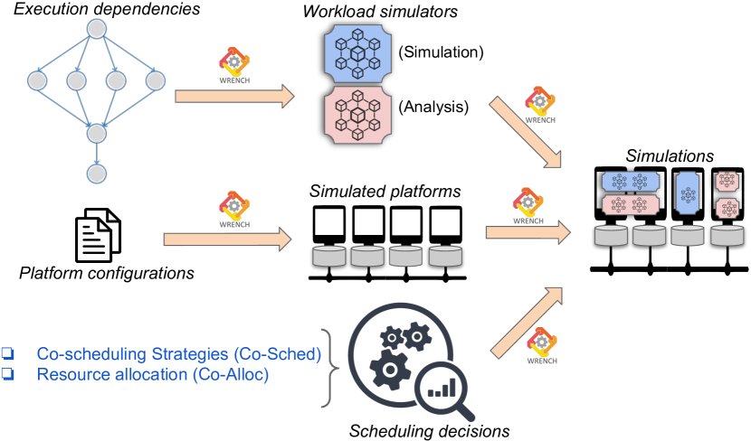
Figure 2: Simulator

V-A Experimental Setup

Setup. The simulator takes the following inputs: (1) a workflow ensemble’s configurations (i.e., number of simulations, number of coupled analyses per simulation, coupling relations), (2) application profiles (i.e., simulations and analyses’ sequential execution times), (3) resources constraints (i.e., number of nodes, number of cores per node, processor speed, network bandwidth), (3) a co-scheduling mapping (i.e., the simulation each analysis is co-scheduled with), and (4) a resource allocation (i.e., number of nodes and cores each application is assigned). We vary the workflow ensemble’s configurations to evaluate the importance and the impact of different configurations on the efficiency of our proposed scheduling choices. We fix the simulations’ profiles, e.g. sequential execution time of the simulations, to study the impact of analyses on scheduling decisions. Sequential execution time of the analyses is generated randomly in a specific range which is relative to the sequential execution time of their coupled simulations. In this experiment, we generate it from $50\%$ to $150\%$ of the simulation’s sequential execution time. Even though our solution is applicable to any data size generated by the simulations, for the sake of simplicity, the amount of data processed by each analysis is kept at a fixed amount among all simulations, even though that amount is varied at different workflow ensemble’s configurations.

Scenarios. We compare a variety of scenarios corresponding to different co-scheduling mappings (see Section V-C). Ideal is the co-scheduling mapping where all analyses are co-scheduled with their respective simulation. In-transit represents the scenario where all analyses are co-scheduled together on a dedicated co-scheduling allocation. We also compose hybrid scenarios where some analyses are co-scheduled with the simulation they couple with while the others are co-scheduled on the co-scheduling allocation without the presence of any simulation. For Increasing-x% (resp. Decreasing-x%), we pick the largest $x\%$ of the analyses, which is sorted in ascending (resp. descending) order of sequential execution time, to not co-schedule with the simulation they couple with (i.e. to co-schedule them on the dedicated co-scheduling allocation). In this evaluation, we consider different percentages of number of analyses, $25\%$, $50\%$, $75\%$. For each of these co-scheduling mappings, we compute the resource allocations for the ensemble using Co-Alloc, which is described in Section IV-B.

V-B Bandwidth Calibration

In order for the simulator to accurately reflect the execution platform, we have to calibrate the bandwidth per node used in our model to improve the precision of our solution using Co-Alloc. In our model, the bandwidth model is simple and optimistic as it does not account for concurrent accesses (i.e., the bandwidth available to each application is the maximum bandwidth $B$). The idea is to compare the makespan given by our performance model (i.e.,  Theorem 3) to the makespan given by our simulation as WRENCH/SimGrid offers pretty complex and accurate communication models. In Figure 3, the theoretical makespan estimated by our model using the maximum bandwidth $B$ exhibits a large difference from the makespan resulted by the simulator (up to 30 times). The simulated bandwidth is smaller than $B$ during the execution as it is shared among concurrent I/O operations. Therefore, we explore different bandwidth values (see Table II) and re-estimate the makespan using our model based on the resource allocation at maximum bandwidth.

Model	Bandwidth
Baseline	$B$
$B^{\prime}_{1}$	$B/|P^{NC}|$
$B^{\prime}_{2}$	$B/\widetilde{N}$
$B^{\prime}_{3}$	$B/(\widetilde{N}\times|P^{NC}|)$

TABLE II: Bandwidth models to calibrate the simulator. $\widetilde{N}$ is number of nodes assigned to analysis in $P^{NC}$.

Figure 3: Makespan estimated by the model for the Increasing-50% scenario with different values of bandwidth per node (see Table II).

Figure 3 confirms our hypothesis that bandwidth is shared among concurrent I/Os and the accuracy of Co-Alloc depends on choosing appropriate bandwidth used in the model. $B^{\prime}_{3}$ provides an approximation that is close to the makespan given by the simulator, we therefore choose $B^{\prime}_{3}$ as the calibrated bandwidth for the experiments hereafter.

V-C Results

In this subsection, we explore the configuration space of the workflow ensemble. We aim to characterize the impact of different co-scheduling strategies by comparing the makespan of the simulator over various scenarios described in Section V-C. To ensure the reliability of results, each value is averaged over 5 trials.

Implications of Co-Sched.

TABLE III: Experimental scenarios, where $A(x\%)$ is the $x\%$ largest analyses’ sequential time of $A$.

Scenarios	Analyses co-scheduled with their coupled simulation ($P^{C}$)	Analyses not co-scheduled with their coupled simulation ($P^{NC}$)
Ideal	A	Ø
In-transit	Ø	A
Increasing-x%	$A\setminus A(x\%)$	$A(x\%)$
Decreasing-x%	$A(100-x\%)$	$A\setminus A(100-x\%)$

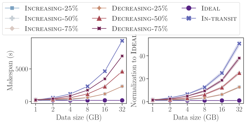
(a) Data size is varying. The workflow ensemble runs on $16$ nodes and has $4$ simulations, $4$ analyses per simulation.

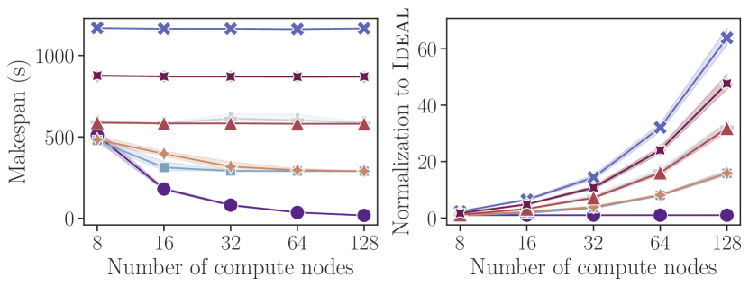
(b) Number of nodes is varying. The workflow ensemble has $4$ simulations, $4$ analyses per simulation. Each analysis processes $4GB$ of data each iteration

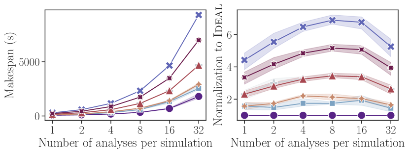
(c) Number of analyses per simulation is varying. The workflow ensemble runs on $16$ nodes and has $4$ simulations. Each analysis processes $4GB$ of data each iteration

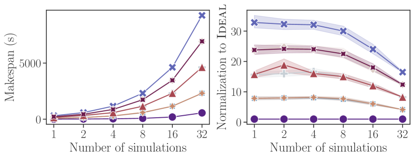
(d) Number of simulations is varying. The workflow ensemble runs on $64$ nodes and has $4$ analyses per simulation. Each analysis processes $4GB$ of data each iteration

Figure 4: Makespan of the workflow ensemble when varying various configurations.

We vary one configuration of the workflow ensemble at a time while keeping the other configurations fixed.  Figure 4(a) shows the makespan of the workflow ensemble running on $16$ nodes with $4$ simulations, $4$ analyses per simulation when varying the size of data processed by each analysis each iteration.  Figure 4(b) is the result with $4$ simulations, $4$ analyses per simulation and $4GB$ of data when varying the number of nodes. In Figure 4(c), the number of analyses per simulation is varied while keeping the number of simulation fixed at $4$ and $4GB$ of data, $4$ analyses per simulation. In Figure 4(d), the number of simulations is varied while keeping the number of analyses per simulation fixed at $4$, $4GB$ of data and $64$ nodes.

Figure 4 demonstrates the following order if the scenarios are sorted in ascending order by their makespan: Ideal, x-25%, x-50%, x-75%, In-transit, where x is either Increasing or Decreasing as those scenarios’ makespan are approximately close to each other. Note that, for Ideal, $0\%$ of the analyses are not co-scheduled with their coupled simulation while that percentage is $100\%$ for In-transit. This observation aligns with our finding in Theorem 1 that not co-scheduling an analysis with its coupled simulation yields a higher makespan. The more number of analyses not co-scheduled with their coupled simulation, the slower the makespan. Since Ideal outperforms the other scenarios, ideal co-scheduling mappings should be favored when the available resources can sustain. In Figures 4(a), 4(c) and 4(d), the makespan scales linearly with the size of data processed by the analyses each iteration, the number of analyses per simulation and the number of simulations, respectively in which Ideal imposes the smallest escalation when these parameters are increased. In Figure 4(b), only the makespan of the Ideal is decreased when the number of nodes is increased. This is because the more nodes are utilized, the more communications are required to exchange the data, which requires the communication bandwidth is shared among them. The communication stages in each step are therefore slower even though the computational stages are faster due to more computing resources are assigned. Only the Ideal which incurs no remote communication can fully take advantage of the available resources.

Efficiency of Co-Alloc.

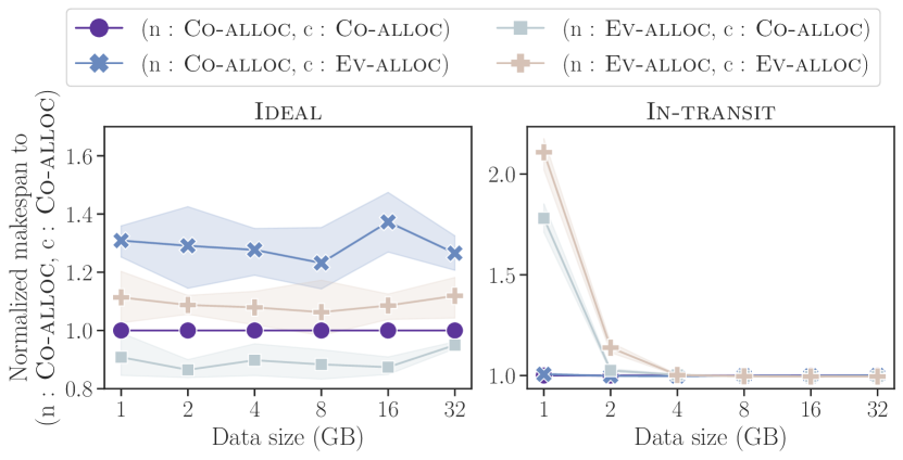
Figure 5: Comparison of normalized makespan of Co-Alloc to Ev-Alloc, where resources are evenly distributed. $(n:\textsc{Co-Alloc},c:\textsc{Ev-Alloc})$ indicates Co-Alloc is applied at node-level while Ev-Alloc is applied at core-level.

We compare the resource allocation computed by Co-Alloc with a naive approach of evenly distributing the resources, which is called as Ev-Alloc. Specifically, at node-level, with Ev-Alloc, the number of nodes is equally divided among co-scheduling allocations while at core-level, for each co-scheduling allocation, the number of cores per node is equally divided among applications co-scheduled in such the allocation. Let $(n:x,c:y)$ is a manner to compute resource allocations, in which we apply $x$ method at node-level while using $y$ method at core-level. We study 4 possible combinations: $(n:\textsc{Co-Alloc},c:\textsc{Co-Alloc})$, $(n:\textsc{Co-Alloc},c:\textsc{Ev-Alloc})$, $(n:\textsc{Ev-Alloc},c:\textsc{Co-Alloc})$, and $(n:\textsc{Ev-Alloc},c:\textsc{Ev-Alloc})$.

Even though the experiment is conducted over all the scenarios in the configuration space, due to the lack of space, we selectively present a subset of scenarios where the allocations significantly differ between observing combinations.  Figure 5 shows the makespan, which is normalized to $(n:\textsc{Co-Alloc},c:\textsc{Co-Alloc})$, in two representative extreme scenarios: Ideal and In-transit when the amount of data processed each iteration is varied. In the Ideal scenario, $(n:\textsc{Co-Alloc},c:\textsc{Co-Alloc})$ surpasses the other combinations, except $(n:\textsc{Ev-Alloc},c:\textsc{Co-Alloc})$. This is because Ideal comprises no remote communication, thus execution time of each application’s step is dominant by the portion of computational stages, which cause the performance is more sensitive to the changes at core-level than at node-level. For In-transit, using Ev-Alloc at node-level results in a slower makespan (up to two times higher) than using Co-Alloc as off-node communications are primary in this scenario. For larger data sizes, the I/O stages take the large proportion in each step in In-transit, which makes the computing time negligible, thus there is no clear difference among discussed combinations.

VI Conclusions

In this paper, we have introduced an execution model of coupling behavior between in situ jobs in a complex workflow ensemble. Based on the proposed model, we theoretically characterized computation and communication characteristics in each in situ component. We further relied on this model to determine co-scheduling policies and resource profiles for each simulation and in situ analysis such that the makespan of the workflow ensemble is minimized under given available computing resources. By evaluating the scheduling solutions via simulation, we validate our proposed approach and confirm its correctness. We are also able to confirm the relevance of data locality as well as the need of well-management shared resources (e.g., bandwidth per node) in co-scheduling concurrent applications together.

For future work, we plan to extend the scheduling model to include contention and interference effects between in situ jobs sharing the same underlying resources. Another promising research direction is to consider more complex use cases leveraging ensembles, e.g. adaptive sampling [31] in which more coordination will be needed to achieve better performance as the simulations are periodically stopped and restarted.

References

- [1] I. Foster et al., “Computing just what you need: Online data analysis and reduction at extreme scales,” in Euro-Par 2017: Parallel Processing. Cham: Springer International Publishing, 2017, pp. 3–19.
- [2] P. Raiteri et al., “Efficient reconstruction of complex free energy landscapes by multiple walkers metadynamics,” The Journal of Physical Chemistry B, vol. 110, no. 8, pp. 3533–3539, 2006.
- [3] J. Comer et al., “Multiple-replica strategies for free-energy calculations in namd: Multiple-walker adaptive biasing force and walker selection rules,” Journal of Chemical Theory and Computation, vol. 10, no. 12, 2014.
- [4] Y. Okamoto, “Generalized-ensemble algorithms: enhanced sampling techniques for monte carlo and molecular dynamics simulations,” Journal of Molecular Graphics and Modelling, vol. 22, no. 5, 2004.
- [5] R. Chelli et al., “Serial generalized ensemble simulations of biomolecules with self-consistent determination of weights,” Journal of Chemical Theory and Computation, vol. 8, no. 3, 2012.
- [6] M. Malawski et al., “Algorithms for cost- and deadline-constrained provisioning for scientific workflow ensembles in iaas clouds,” Future Generation Computer Systems, vol. 48, pp. 1–18, 2015.
- [7] D. H. Ahn et al., “Flux: Overcoming scheduling challenges for exascale workflows,” Future Generation Computer Systems, vol. 110, pp. 202–213, 2020.
- [8] J. L. Peterson et al., “Enabling machine learning-ready hpc ensembles with merlin,” Future Generation Computer Systems, 2022.
- [9] P. Malakar et al., “Optimal execution of co-analysis for large-scale molecular dynamics simulations,” in SC ’16: Proceedings of the International Conference for High Performance Computing, Networking, Storage and Analysis, 2016, pp. 702–715.
- [10] G. Aupy et al., “Modeling high-throughput applications for in situ analytics,” The International Journal of High Performance Computing Applications, vol. 33, no. 6, pp. 1185–1200, 2022/03/01 2019.
- [11] M. Taufer et al., “Characterizing in situ and in transit analytics of molecular dynamics simulations for next-generation supercomputers,” in 2019 15th International Conference on eScience (eScience), 2019, pp. 188–198.
- [12] J. Breitbart et al., “Dynamic co-scheduling driven by main memory bandwidth utilization,” in 2017 IEEE International Conference on Cluster Computing (CLUSTER), 2017, pp. 400–409.
- [13] F. V. Zacarias et al., “Intelligent colocation of workloads for enhanced server efficiency,” in 2019 31st International Symposium on Computer Architecture and High Performance Computing (SBAC-PAD), 2019, pp. 120–127.
- [14] R. Kuchumov et al., “Analytical and numerical evaluation of co-scheduling strategies and their application,” Computers, vol. 10, no. 10, 2021.
- [15] C. Sewell et al., “Large-scale compute-intensive analysis via a combined in-situ and co-scheduling workflow approach,” in Proceedings of the International Conference for High Performance Computing, Networking, Storage and Analysis, ser. SC ’15. New York, NY, USA: Association for Computing Machinery, 2015.
- [16] G. Aupy et al., “Co-scheduling hpc workloads on cache-partitioned cmp platforms,” in 2018 IEEE International Conference on Cluster Computing (CLUSTER), 2018, pp. 348–358.
- [17] T. M. A. Do et al., “Performance assessment of ensembles of in situ workflows under resource constraints,” Concurrency and Computation: Practice and Experience, vol. n/a, no. n/a, p. e7111, 2022/07/11 2022.
- [18] T. Johnston et al., “In situ data analytics and indexing of protein trajectories,” Journal of Computational Chemistry, vol. 38, no. 16, pp. 1419–1430, 2022/07/14 2017.
- [19] D. Dauwe et al., “Modeling the effects on power and performance from memory interference of co-located applications in multicore systems,” in International Conference on Parallel and Distributed Processing Techniques and Applications (PDPTA), 1 2014.
- [20] T. M. A. Do et al., “A lightweight method for evaluating in situ workflow efficiency,” Journal of Computational Science, vol. 48, p. 101259, 2021.
- [21] G. M. Amdahl, “Validity of the single processor approach to achieving large scale computing capabilities,” in Proceedings of the April 18-20, 1967, Spring Joint Computer Conference, ser. AFIPS ’67. New York, NY, USA: Association for Computing Machinery, 1967, p. 483–485.
- [22] M. Herlihy et al., The Art of Multiprocessor Programming, Revised Reprint, 1st ed. San Francisco, CA, USA: Morgan Kaufmann Publishers Inc., 2012.
- [23] T. M. A. Do et al., “Enabling data analytics workflows using node-local storage,” in International Conference for High Performance Computing, Networking, Storage, and Analysis (SC18), Dallas, TX, 2018.
- [24] H. Kim et al., “Understanding energy aspects of processing-near-memory for hpc workloads,” in Proceedings of the 2015 International Symposium on Memory Systems, ser. MEMSYS ’15. New York, NY, USA: Association for Computing Machinery, 2015, p. 276–282.
- [25] S. Williams et al., “Roofline: An insightful visual performance model for multicore architectures,” Commun. ACM, vol. 52, no. 4, p. 65–76, Apr. 2009.
- [26] D. G. Feitelson, “Job scheduling in multiprogrammed parallel systems,” 1997.
- [27] M. Stillwell et al., “Resource allocation algorithms for virtualized service hosting platforms,” Journal of Parallel and Distributed Computing, vol. 70, no. 9, pp. 962–974, 2010.
- [28] H. Casanova et al., “Developing Accurate and Scalable Simulators of Production Workflow Management Systems with WRENCH,” Future Generation Computer Systems, vol. 112, pp. 162–175, 2020.
- [29] ——, “Versatile, scalable, and accurate simulation of distributed applications and platforms,” Journal of Parallel and Distributed Computing, vol. 74, no. 10, pp. 2899–2917, 06 2014.
- [30] T. M. A. Do et al., “A lightweight method for evaluating in situ workflow efficiency,” Journal of Computational Science, vol. 48, 2021.
- [31] V. Balasubramanian et al., “Adaptive ensemble biomolecular applications at scale,” SN Computer Science, vol. 1, no. 2, p. 104, 2020.