Measuring Friendship Closeness: A Perspective of Social Identity Theory

Abstract.

Measuring the closeness of friendships is an important problem that finds numerous applications in practice. For example, online gaming platforms often host friendship-enhancing events in which a user (called the source) only invites his/her friend (called the target) to play together. In this scenario, the measure of friendship closeness is the backbone for understanding source invitation and target adoption behaviors, and underpins the recommendation of promising targets for the sources. However, most existing measures for friendship closeness only consider the information between the source and target but ignore the information of groups where they are located, which renders inferior results. To address this issue, we present new measures for friendship closeness based on the social identity theory (${\mathsf{SIT}}$), which describes the inclination that a target endorses behaviors of users inside the same group. The core of ${\mathsf{SIT}}$ is the process that a target assesses groups of users as them or us. Unfortunately, this process is difficult to be captured due to perceptual factors. To this end, we seamlessly reify the factors of ${\mathsf{SIT}}$ into quantitative measures, which consider local and global information of a target’s group. We conduct extensive experiments to evaluate the effectiveness of our proposal against 8 state-of-the-art methods on 3 online gaming datasets. In particular, we demonstrate that our solution can outperform the best competitor on the behavior prediction (resp. online target recommendation) by up to 23.2% (resp. 34.2%) in the corresponding evaluation metric.

1. Introduction

Consider a social network $\mathcal{G}=(\mathcal{V},\mathcal{E})$, where each node $v_{s}\in\mathcal{V}$ represents the user $v_{s}$ and each edge $(v_{s},v_{t})\in\mathcal{E}$ represents the friendship of two users $v_{s}$ and $v_{t}$. Measuring the closeness of the friendship $(v_{s},v_{t})$ is an important problem and finds numerous applications in real-world scenarios, where a user $v_{s}$ (called the source) only interacts with the friend $v_{t}$ (called the target). For example, online gaming platforms often host friendship-enhancing events, which encourage the source $v_{s}$ to invite the target $v_{t}$ to return to the game or play together (Luo et al., 2019, 2020). In this scenario, the friendship closeness measure is the backbone for understanding the invitation (resp. adoption) behavior of $v_{s}$ (resp. $v_{t}$). Furthermore, this measure can be applied in recommending promising targets for the sources because the number of targets of a source could be considerable. Analogously, in the instant messaging platform WeChat, a source’s post can only be liked and commented on by the target in contacts (Zhang et al., 2018), thus the friendship closeness measure can also be leveraged to predict corresponding activities (Zhang et al., 2021; Sankar et al., 2020; Gomez-Rodriguez et al., 2011).

In the present work, we focus on the topological friendship closeness (${\mathtt{TFC}}$) measure that reflects the closeness of a source-target pair $(v_{s},v_{t})$ on $\mathcal{G}$ rather than labels associated with them. In particular, most existing ${\mathtt{TFC}}$ measures (Adamic and Adar, 2003; Page et al., 1999; Jeh and Widom, 2002; Granovetter, 1978; Fang et al., 2014; Perozzi et al., 2014; Grover and Leskovec, 2016; Yang et al., 2020; Roweis and Saul, 2000; Tang et al., 2015; Wang et al., 2016) adopt the structural information between two users $v_{s}$ and $v_{t}$. For example, (Fang et al., 2014) directly employs the tie strength of $(v_{s},v_{t})$, which is measured by the times of historical interactions; (Adamic and Adar, 2003) proposes several measures in terms of the common neighborhood of $(v_{s},v_{t})$. Furthermore, some measures preserve long and intricate paths between $(v_{s},v_{t})$ based on random walks, e.g., personalized PageRank (Page et al., 1999). Unfortunately, the above-said measures may render compromised results, as they ignore the group information and the potential group effect related to $(v_{s},v_{t})$, which says a user’s belonging group can influence his/her decision.

Even though some ${\mathtt{TFC}}$ measures (Soundarajan and Hopcroft, 2012; Epasto et al., 2015; Ugander et al., 2012; Song et al., 2020; Barbieri et al., 2014; De et al., 2016) attempt to take the group effect into consideration, the involved information is still inadequate. To explain, we find that these measures typically require (i) first representing the affiliation relationship between users and groups as a bipartite graph, where users and groups are two disjoint sets of nodes and affiliation relationships are a set of edges, and (ii) then exploiting information on this bipartite graph. For example, (Ugander et al., 2012) proposes structural diversity to measure the number of adjacent groups for a given user; (Song et al., 2020; Barbieri et al., 2014; De et al., 2016) utilize edge weights between users and groups; (Soundarajan and Hopcroft, 2012; Epasto et al., 2015) measures the commonality of groups between two users on this bipartite graph. However, in these works, contracting a group into a node makes more detailed group information imperceptible, e.g., connectivity.

To mitigate the deficiencies of existing measures, we propose to explore the group effect by leveraging the social identity theory (${\mathsf{SIT}}$), which is a fundamental concept in social psychology and is widely applied in domains of human health (Scheepers and Ellemers, 2019), team sports (Rees et al., 2015), computer-supported cooperative works (Seering et al., 2018) and fake news detection (Shu et al., 2017). ${\mathsf{SIT}}$ describes that a target $v_{t}$ tends to endorse attitudes and behaviors of groups of users, who are assessed as us in $v_{t}$’s cognition. In other words, given a target $v_{t}$ and an identified group $\mathcal{C}$ of $v_{t}$, $v_{t}$ is more likely to adopt the invitation from the source $v_{s}\in\mathcal{C}$. Unfortunately, the identification process is difficult to be quantified due to perceptual factors. To this end, we seamlessly reify the factors of ${\mathsf{SIT}}$ into ${\mathtt{TFC}}$ measures, which consider a group’s local and global information. For example, by modeling the social network as a physical system, we propose to measure the attractive spring-like force related to a group, in which the information of group connectivity and in-group user homogeneity are naturally incorporated. In contrast, previous ${\mathtt{TFC}}$ measures only consider similarities of group memberships (Soundarajan and Hopcroft, 2012; Epasto et al., 2015).

We experimentally evaluate the proposed ${\mathsf{SIT}}$-based solution against 8 representative competitors on 3 real-world online game datasets. In particular, we demonstrate that the proposed solution outperforms all competitors in terms of AUC, accuracy, and F1 score while predicting target adoption and source invitation behaviors on the tested dataset. Besides, we detailedly analyze the relations between user behaviors and ${\mathsf{SIT}}$ factors, and the importance of these factors. At last, we deploy our solution to the online target recommendation, which achieves up to 34.2% improvement over the best treatment in the corresponding evaluation metric.

To summarize, we make the following contributions in this work:

• We propose new ${\mathtt{TFC}}$ measures based on ${\mathsf{SIT}}$ in social psychology, which preserve both local and global information of groups.

• We conduct extensive experiments and analysis to demonstrate the superiority of proposed ${\mathsf{SIT}}$-based ${\mathtt{TFC}}$ measures over state-of-the-art competitors while predicting user behaviors.

• We deploy the presented solution to the online target recommendation, which achieves significant improvement.

2. Preliminaries

In this section, we first elaborate on the problem of measuring the topological friendship closeness (${\mathtt{TFC}}$), followed by the illustration of main competitors and downstream tasks that ${\mathtt{TFC}}$ measures are to solve in this work. At last, we introduce the background of the social identity theory.

2.1. Problem Formulation

Let $\mathcal{G}=(\mathcal{V},\mathcal{E})$ be a social network, where $\mathcal{V}$ is a set of users (called nodes) and $\mathcal{E}$ is a set of friendships (called edges). We assume that the friendship $(v_{s},v_{t})\in\mathcal{E}$ is directed and is associated with an edge weight $w_{s,t}\in(0,1]$. Given a directed edge $(v_{s},v_{t})\in\mathcal{E}$, we call $v_{s}$ (resp. $v_{t}$) the source (resp. target) neighbor of $v_{t}$ (resp. $v_{s}$). Given a node $v_{t}\in\mathcal{V}$, the source neighborhood of $v_{t}$ consists of: (i) $v_{t}$ itself; (ii) the node set $\mathcal{N}_{t}$, which contains sources of $v_{t}$; (iii) the edge set $\mathcal{E}_{t}$, which contains the edge $(v_{s},v_{t})\in\mathcal{E}$; (iv) the edge set $\mathcal{R}_{t}$, which contains the edge $(v_{s},v_{k})\in\mathcal{E}$ between sources $v_{s},v_{k}\in\mathcal{N}_{t}$.

Recall in Section 1 that, given an input social network $\mathcal{G}$, the ${\mathtt{TFC}}$ measure reflects the topological closeness for each $(v_{s},v_{t})\in\mathcal{E}$. Given a source-target pair $(v_{s},v_{t})\in\mathcal{E}$, the goal of our present work is to design the ${\mathtt{TFC}}$ measure, which leverages the structural information of the group $\mathcal{C}$, where $v_{s},v_{t}\in\mathcal{C}$. For simplicity, we assume that $v_{s}$ and $v_{t}$ are only co-located in one group $\mathcal{C}$. As for the partitioning of groups, it relies on the social identity theory and will be illustrated in Section 3.

2.2. Main Competitors

In what follows, we briefly elaborate on the main ideas of competing ${\mathtt{TFC}}$ measures in the present work. For better clarity, we call a measure as the group-level ${\mathtt{TFC}}$ measure if considering the group information, and the individual-level ${\mathtt{TFC}}$ measure otherwise. Specifically, we select 5 representative individual-level measures: tie strength (Tang et al., 2015; Fang et al., 2014), number of common neighbors (Tang et al., 2015; Adamic and Adar, 2003), personalized PageRank (Page et al., 1999), cosine and euclidean similarity of Node2Vec vectors (Grover and Leskovec, 2016); 3 commonly-used group-level measures: structural diversity (Ugander et al., 2012), user-group tie strength (Song et al., 2020) and group edge density (Purohit et al., 2014). It is worth noting that the selected individual-level measures are also known as proximities (Cai et al., 2018; Tang et al., 2015), which can reflect the topological closeness for all node pairs. Furthermore, these ${\mathtt{TFC}}$ measures are widely applied in Tencent gaming platforms (Luo et al., 2019, 2020).

Tie strength. Given a friendship $(v_{s},v_{t})\in\mathcal{E}$, the tie strength equals to the edge weight $w_{s,t}$ (Tang et al., 2015; Fang et al., 2014).

Number of common neighbors. Given a friendship $(v_{s},v_{t})\in\mathcal{E}$, this measure counts the number of common neighbors (Tang et al., 2015; Adamic and Adar, 2003) of source $v_{s}$ and target $v_{t}$, which can reflect the similarity of two node’s local structure.

Personalized PageRank. Given a friendship $(v_{s},v_{t})\in\mathcal{E}$, this measure aims to preserve intricate topological relations between nodes by performing random walks. In particular, the personalized PageRank (Page et al., 1999) from $v_{s}$ to $v_{t}$ is defined as the probability that a random walk with restart (RWR) (Tong et al., 2006) originating from $v_{s}$ stops at $v_{t}$. The corresponding RWR starts from the source $v_{s}$ and, in each step, chooses to (i) either terminate at the current node with probability $\alpha$, (ii) or navigate to a random target neighbor of the current node with the remaining $1-\alpha$ probability.

Similarity of Node2Vec vectors. As a node embedding method (Cai et al., 2018), Node2Vec (Grover and Leskovec, 2016) proposes to represent each node $v_{s}\in\mathcal{G}$ as a compact vector, which preserves the structural information in the vicinity of $v_{s}$. By this method, given a friendship $(v_{s},v_{t})\in\mathcal{E}$, the ${\mathtt{TFC}}$ can be measured by the cosine similarity or euclidean distance between the Node2Vec vectors of $v_{s}$ and $v_{t}$. Compared with the prior work DeepWalk (Perozzi et al., 2014), the core contribution of Node2Vec is that it takes two-order random walks as inputs for training. Compared with the RWR, the two-order random walk will not terminate until a pre-defined length limit. Moreover, given the current node $v_{j}$, the target neighbors of $v_{j}$ are first divided into the following three categories: (i) the source neighbor $v_{i}$ that was visited in the previous step, (ii) $v_{k}$ that is the common target neighbor of $v_{i}$ or (iii) otherwise. Then different (resp. same) transition probabilities are assigned to nodes across (resp. inside) each category. At last, the next node of this walk is selected in terms of the biased probability.

Structural diversity. Ugander et al. are the first to propose the concept of structural diversity (Ugander et al., 2012), which is further applied for influence analysis (Fang et al., 2014; Zhang et al., 2021; Su et al., 2020; Qiu et al., 2016). Specifically, given a friendship $(v_{s},v_{t})\in\mathcal{E}$, the ${\mathtt{TFC}}$ measure based on the structural diversity equals to the number of weakly connected components (see Definition 2.1) in a subgraph, which is derived from $v_{t}$’s source neighbors affected by a specific event and their relationships. This work (Ugander et al., 2012) points out that a more extensive structural diversity of $v_{t}$ indicates a higher probability that $v_{t}$ will be influenced.

Definition 2.1 (Weakly Connected Component).

Given a directed graph, a weakly connected component is a maximal subgraph, where any inside node is connected by paths if ignoring the direction of edges.

User-group tie strength. Given a friendship $(v_{s},v_{t})\in\mathcal{E}$ and a group $\mathcal{C}$ where $v_{s},v_{t}\in\mathcal{C}$, the ${\mathtt{TFC}}$ measure based on the user-group tie strength (Song et al., 2020; Barbieri et al., 2014; De et al., 2016) equals to the summation of tie strength between $v_{t}$ and other members in $\mathcal{C}$.

Group edge density. Given a friendship $(v_{s},v_{t})\in\mathcal{E}$ and a group $\mathcal{C}$ where $v_{s},v_{t}\in\mathcal{C}$, the ${\mathtt{TFC}}$ measure based on the group edge density is defined as the fraction of the summation of edge weights in $\mathcal{C}$ over the number of all possible edges in $\mathcal{C}$, which is also applied to analyze group dynamics (Purohit et al., 2014; Qiu et al., 2016).

2.3. Downstream Tasks

Before introducing downstream tasks, we first illustrate friendship-enhancing events in Tencent‘s online gaming platforms, whose procedure is as follows. First, given a social network $\mathcal{G}=(\mathcal{V},\mathcal{E})$, a source set $\mathcal{S}\subseteq\mathcal{V}$ and a target set $\mathcal{T}\subseteq\mathcal{V}$ are selected regarding the event demand, e.g., recalling inactive targets and stimulating interactions between friends. Then, the event is sent to each source $v_{s}\in\mathcal{S}$, and allows $v_{s}$ to invite the target neighbor $v_{t}\in\mathcal{T}$ from a feed window with at most $k$ target friends. Once a target $v_{t}$ adopts the invitation from the source $v_{s}$, both $v_{s}$ and $v_{t}$ will receive virtual gifts as incentives. To summarize, there exist two types of user activities: source invitation and target adoption. In friendship-enhancing events, ${\mathtt{TFC}}$ measures act as structural heuristics to facilitate the understanding of invitation and adoption behaviors and recommending targets for the sources, which are defined as follows.

Problem 1 (Behavior prediction).

Given a graph $\mathcal{G}=(\mathcal{V},\mathcal{E})$ and a source-target pair $(v_{s},v_{t})\in\mathcal{E}$, the objective of behavior prediction is to infer the likelihood that source invitation and target adoption behaviors happen between $(v_{s},v_{t})$.

Problem 2 (Target recommendation).

Given a graph $\mathcal{G}=(\mathcal{V},\mathcal{E})$, a budget $k$, a source set $\mathcal{S}$ and a target set $\mathcal{T}$, the objective of target recommendation is to select at most $k$ target neighbors from $\mathcal{T}$ for each source user $v_{s}\in\mathcal{S}$, such that the likelihood that both invitation and adoption behaviors happen among all returned source-target pairs are maximized.

2.4. Social Identity Theory

Formulation. Turner and Tajfel define social identity as ‘the individual’s knowledge that he/she belongs to certain social groups together with some emotional and value significance to him of this group membership’ (Tajfel and Turner, 2004). In other words, social identity theory (${\mathsf{SIT}}$) emphasizes how the target user’s belonging group affects his/her behavior. Given a social network $G$ and a target $v_{t}$, ${\mathsf{SIT}}$ is formulated by three cognitive processes: categorization, identification and comparison (Tajfel and Turner, 2004). Specifically, the categorization is a preprocessing step, which partitions the users of $\mathcal{G}$ into several candidate social groups w.r.t $v_{t}$. In the identification stage, $v_{t}$ will identify him/herself as a member of a certain candidate group. Finally, the comparison stage says that, for the sake of self-esteem, $v_{t}$ tends to shift the sense of belonging based on group social standing.

Table 1. Factors in $\boldsymbol{\mathsf{SIT}}$.

Factor	Meaning
Multi-membership	Number of groups
Inclusiveness	Number of in-group members
Satisfaction	$v_{t}$’s feelings about being a group member
Solidarity	$v_{t}$’s psychological bond with in-group members
Centrality	Importance of a group in $v_{t}$’s cognition
Self-stereotyping	Similarity of $v_{t}$ and group average in $v_{t}$’s cognition
In-group homogeneity	Similarity within a group
Social standing	Social standing of a group

Factors. After pre-partitioning candidate groups for a target $v_{t}$, both identification and comparison stages depend on many factors. We summarize the factors used in this paper in Table 1. Specifically, to understand the identification stage, the statistical factors multi-membership (Sieber, 1974) and inclusiveness (Brewer and Gardner, 1996) are proposed. Besides, Leach et al. (Leach et al., 2008) extensively summarize existing social perceptual factors as: satisfaction (Tajfel and Turner, 2004; Cameron, 2004), solidarity (Cameron, 2004; Doosje et al., 1998), centrality (Cameron, 2004; Doosje et al., 1998; Brewer and Gardner, 1996), self-stereotyping (Oakes et al., 1994; Simon, 1992) and in-group homogeneity (Oakes et al., 1994; Simon, 1992). Regarding the comparison stage, by definition, the social standing of a group is also recognized as a pivotal factor (Tajfel and Turner, 2004).

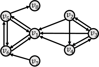
(a)

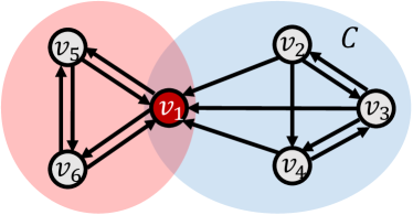
(b)

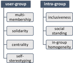
(c)

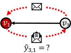
(d)

Figure 1. Illustration of core subroutines.

3. Overview

We illustrate the main workflow of the present work in Figure 1, which processes the input graph by following three steps.

Step 1: categorization. For employing ${\mathsf{SIT}}$, the first step is partitioning candidate groups for each target user, i.e., the categorization stage. To explore the group information for the source-target pair, given a graph $\mathcal{G}=(\mathcal{V},\mathcal{E})$ and a target user $v_{t}$, we partition the source neighborhood of $v_{t}$ based on the weakly connected components (see Definition 2.1). Specifically, following operations in (Ugander et al., 2012; Fang et al., 2014; Zhang et al., 2021; Epasto et al., 2015), we first extract each weakly connected component (dubbed as ${\mathsf{CC}}$) from the ego network $\mathcal{G}_{t}=(\mathcal{N}_{t},\mathcal{R}_{t})$ of $v_{t}$, and then call all sources in a given ${\mathsf{CC}}$ and the target $v_{t}$ as a candidate group $\mathcal{C}$, since $v_{t}$ connects to all sources in the ${\mathsf{CC}}$ by edges in $\mathcal{E}_{t}$. To exemplify, given an input graph as shown in Figure 1(a), the source neighborhood of target node $v_{1}$ is partitioned into two candidate groups (shaded in two colors in Figure 1(b)), among which the group $\mathcal{C}$ is constituted by $v_{1},v_{2},v_{3},v_{4}$. The rationale for employing ${\mathsf{CC}}$ is two-fold. First, as suggested in ${\mathsf{SIT}}$ (Gaertner and Dovidio, 2014), the candidate group requires to be categorized in a more general way to mitigate the in-group bias. For instance, employers in two departments of the same company should be categorized into one company group rather than split into two department groups. By definition, the ${\mathsf{CC}}$ can satisfy this requirement, as the inside nodes of two ${\mathsf{CCs}}$ are isolated (i.e., no path). Second, ${\mathsf{CC}}$ is a simple but effective way to represent the community in the ego network of a user (Epasto et al., 2015; Yang and Leskovec, 2015). As evidence, (Epasto et al., 2015) finds that employing ${\mathsf{CCs}}$ for the link prediction can achieve comparable or even slightly better performance than employing communities detected by the state-of-the-art methods.

Step 2: $\boldsymbol{\mathsf{SIT}}$-based measure definition. As shown in Figure 1(c), factors of ${\mathsf{SIT}}$ in Table 1 can be separated into two branches: (i) user-group factors, describing the information between the target and other members; (ii) intra-group factors, describing the stand-alone information of other members. For example, the factors of self-stereotyping and in-group homogeneity both focus on individual similarities, however, by definition, the former is a user-group factor and the latter is an intra-group one. Accordingly, once the categorization stage is accomplished, given a target $v_{t}$ and a candidate group $\mathcal{C}$, the second step is to devise group-level measures between $v_{t}$ and $\mathcal{C}\backslash v_{t}$ (resp. among sources in $\mathcal{C}\backslash v_{t}$) to quantify user-group (resp. intra-group) factors of ${\mathsf{SIT}}$. Notice that we skip the satisfaction factor as it involves numerous human sentiments and is difficult to be detected by employing graph topology only.

Step 3: Inclination inference. In the third step, we employ the proposed ${\mathsf{SIT}}$-based measures to infer the inclination that the target $v_{t}$ endorses each candidate group $\mathcal{C}$. This inclination is defined as

$$\hat{y}_{\mathcal{C},t}=\frac{\sum_{v_{s}\in\mathcal{C}\backslash v_{t}}\hat{y}_{s,t}}{|\mathcal{C}|-1},$$

where $|\mathcal{C}|\geq 2$ as there exist at least $v_{t}$ and a source, and $\hat{y}_{s,t}$ is the likelihood that $v_{t}$ adopts the invitation from each source $v_{s}$ in $\mathcal{C}$ (see Figure 1(d)) and can be applied in the downstream Problem 1 and Problem 2. Without loss of generality, we derive $\hat{y}_{s,t}$ by a supervised manner, which works as follows. For each training source-target pair $(v_{s},v_{t})$, we first take the proposed ${\mathsf{SIT}}$-based measures as $d$-dimensional features $x_{s,t}\in\mathbb{R}^{d}$ and $y_{s,t}\in\{0,1\}$ as the label of the adoption behavior, where $y_{s,t}=1$ indicates $v_{t}$ adopts the invitation from $v_{s}$ and $y_{s,t}=0$ otherwise. We next train a well-accepted ${\mathsf{XGBoost}}$ (Chen and Guestrin, 2016) model, which is finally utilized to infer each $\hat{y}_{s,t}$. Specifically, given a training dataset with related tuple $(x_{s,t},y_{s,t})$ and $T$ regression trees with the maximum depth $h$, ${\mathsf{XGBoost}}$ aims to find the best parameters attached on all possible $2^{h}$ leaves of each of $T$ trees by the following objective where all parameters are represented by a matrix $\mathbf{\Theta}\in\mathbb{R}^{T\times 2^{h}}$,

(1) $$\underset{\mathbf{\Theta}}{\operatorname{arg}\,\operatorname{min}}\;\left(\mathcal{L}(\mathbf{\Theta})+\Omega(\mathbf{\Theta})\right).$$

In Eq.(1), the training loss term is defined as the logistic loss

(2) $$\mathcal{L}(\mathbf{\Theta})=\sum\limits_{s,t}\left(y_{s,t}\ln(1+e^{-\hat{y}_{s,t}})+(1-y_{s,t})\ln(1+e^{\hat{y}_{s,t}})\right),$$

and the regularization term $\Omega(\mathbf{\Theta})$ considers both L0 and L2 norms of $\mathbf{\Theta}$. Regarding the predicted value $\hat{y}_{s,t}$ in Eq.(2), it aggregates the parameters by $\hat{y}_{s,t}=\sum_{i}\mathbf{\Theta}[i,q_{i}(s,t)]$, where the $i$-th row of $\mathbf{\Theta}$ contains all parameters in the $i$-th tree and $q_{i}(s,t)$ is the column index that contains the parameter of current $(v_{s},v_{t})$ in the $i$-th tree. The reason of employing ${\mathsf{XGBoost}}$ is that (i) it is an empirically-efficient solver (Chen and Guestrin, 2016) and is widely accepted for massive game data in Tencent; (ii) the model is easy to be interpreted and is further applied for related analysis in Section 5.2.

Remarks. In what follows, we focus on defining ${\mathsf{SIT}}$-based measures in Section 4, where our key contributions come from. The performance of two downstream tasks are evaluated in Section 5.2 and Section 5.3. As selections of community detection method in step 1 and training model in step 3 are orthogonal to our work, we refer the interested readers to  (Epasto et al., 2015) for the benchmark of different community detection methods and (Chen and Guestrin, 2016) for the detailed training procedure of ${\mathsf{XGBoost}}$, respectively.

4. $\boldsymbol{\mathsf{SIT}}$-based Measures

In this part, we devise the formulation for ${\mathsf{SIT}}$ factors and illustrate their rationales compared with existing group-level measures.

4.1. Multi-membership and Inclusiveness

Inspired from the structural diversity (Ugander et al., 2012), we utilize the number of candidate groups and the size of each group of a target to represent the statistical factors of multi-membership and inclusiveness, respectively. In particular, given a graph $\mathcal{G}$ and a target user $v_{t}$, we define the multi-membership of $v_{t}$ as the number of candidate groups ($\#\mathsf{CC}$) consisting of all source neighbors of $v_{t}$, and the inclusiveness of a given group $\mathcal{C}$ as the group size (${\mathsf{GS}}$), i.e., the cardinality $|\mathcal{C}|$. In contrast, the prior work of structural diversity (Ugander et al., 2012) focuses on the groups with source neighbors who have sent the invitation only.

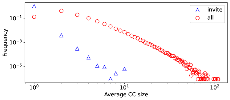
Figure 2. Distribution of averaged $\boldsymbol{\mathsf{CC}}$ size in FPS.

The rationales are as follows. First, before the release time of a given event, invitation behaviors of source users are unknown, and hence corresponding ego networks fail to be extracted. Second, even though the ego networks may be constructed by exploiting source behaviors from historical events, however, the invitation behaviors are only triggered by a small number of source users, which renders a much sparser ego network with many singleton ${\mathsf{CCs}}$ (i.e., one inside member) (Ugander et al., 2012) and makes less group information revealed. For example, Figure 2 shows the distributions of averaged ${\mathsf{CC}}$ size of invited target users on FPS dataset, in which averaged ${\mathsf{CC}}$ size of a target $v_{t}$ equals the fraction of the number of all (or inviting) source neighbors over $\#$${\mathsf{CC}}$ of $v_{t}$. Specifically, by using the inviting source nodes, the resulting distribution in blue triangles is highly-skewed, where singletons are over 99%. In contrast, by using all source neighbors, the results in red circles show an improvement w.r.t the average size, which reveals more group information.

4.2. Social Standing and Centrality

Recall in Section 2.4 that factors of social standing and centrality in ${\mathsf{SIT}}$ describe the group importance in the whole graph and a given target’s cognition, which can be quantified by PageRank and personalized PageRank (PPR), respectively. Given a graph $\mathcal{G}$ with $|\mathcal{V}|=n$ and a restart probability $\alpha$, the PageRank vector of $\mathcal{G}$ is denoted as a vector $\boldsymbol{\Pi}\in\mathbb{R}^{1\times n}$, where the $i$-the column value $\boldsymbol{\Pi}[i]={\rho}_{i}$ is the PageRank value of $v_{i}$. The PageRank vector $\boldsymbol{\Pi}$ satisfies the following equation

(3) $$\boldsymbol{\Pi}=\sum_{t=0}^{\infty}{\alpha(1-\alpha)^{t}\mathbf{s}\cdot\mathbf{P}^{t}},$$

where $\boldsymbol{s}\in\mathbb{R}^{1\times n}$ is the starting vector with the $i$-th column value $\mathbf{s}[i]=1/n$ for each $v_{i}\in\mathcal{V}$. In Eq.(3), $\mathbf{P}\in\mathbb{R}^{n\times n}$ is the probability transition matrix of $G$ where the value in the $i$-th row and $j$-th column is $\mathbf{P}{[i,j]}={1}/{d_{i}}$ for $(v_{i},v_{j})\in\mathcal{E}$ and $\mathbf{P}{[i,j]}=0$ otherwise, where $d_{i}$ is the number of target neighbors of $v_{i}$. Correspondingly, a PPR vector $\mathbf{\Pi}_{i}\in\mathbb{R}^{1\times n}$ w.r.t the user $v_{i}$ can be derived by setting the starting vector $\mathbf{s}$ of Eq.(3) to an one-hot vector where $\mathbf{s}[i]=1$ for $v_{i}$ and $\mathbf{s}[i]=0$ otherwise. The value in the $j$-th column $\mathbf{\Pi}_{i}[j]=\pi_{i,j}$ is the PPR value of $v_{j}$ w.r.t $v_{i}$.

To encapsulate PageRank and PPR into social identity features, we bring the idea from (Everett and Borgatti, 1999) which proposed to measure the group centrality by taking the average centrality scores of in-group members. In particular, we define group PageRank (${\mathsf{GPR}}$) and group personalized PageRank (${\mathsf{GPPR}}$) as follows.

Definition 4.1 (Group PageRank).

Given a graph $\mathcal{G}$, a target user $v_{t}$ and a candidate group $\mathcal{C}$, the group PageRank of $\mathcal{C}$ is defined as

$$\rho_{\mathcal{C}}=\frac{1}{|\mathcal{C}|-1}\sum\limits_{v_{j}\in\mathcal{C}\backslash v_{t}}{\rho}_{j}.$$

Definition 4.2 (Group Personalized PageRank).

Given a graph $\mathcal{G}$, a target user $v_{t}$ and a candidate group $\mathcal{C}$, the group personalized PageRank of $\mathcal{C}$ w.r.t $v_{t}$ is defined as

$$\pi_{t,\mathcal{C}}=\frac{1}{|\mathcal{C}|-1}\sum\limits_{v_{j}\in\mathcal{C}\backslash v_{t}}{\pi}_{t,j}.$$

To understand the intuitions behind ${\mathsf{GPR}}$ and ${\mathsf{GPPR}}$, the PageRank $\rho_{j}$ (resp. PPR $\pi_{t,j}$) in Definition 4.1 (resp. Definition 4.2) can be interpreted as measuring the global importance and social status of in-group member $v_{j}$ (Song et al., 2007; Wu et al., 2016) (resp. relative importance of $v_{j}$ w.r.t $v_{t}$ (Yang et al., 2020)) by performing the RWR as illustrated in Section 2.2. More concrete, $\rho_{j}$ represents the probability that an RWR starting from a randomly-selected node stops at $v_{j}$. In the meantime, $\pi_{t,j}$ also represents the probability that an RWR stops at $v_{j}$, but the starting node is the given node $v_{t}$. Thus, ${\mathsf{GPR}}$ and ${\mathsf{GPPR}}$ can indicate the group importance in terms of the probability that a specific RWR terminates in a given group.

Another possible definition for group importance is to replace (personalized) PageRank with the out-degree centrality. However, compared with PageRank, the out-degree centrality $d_{i}$ of a node $v_{i}$ only considers the one-hop structural information surrounding $v_{i}$, which fails to extensively capture the importance of $v_{i}$ in the whole graph. Besides the above definitions, (Everett and Borgatti, 1999) also suggests aggregating importance scores of in-group members by summation. Nevertheless, grouping by summation imports the bias from the group scale and yields a misleading high ${\mathsf{GPR}}$ and ${\mathsf{GPPR}}$ scores for the group, in which many users contain but the importance of each is tiny, as justified in Section 5.2.

4.3. Solidarity, Self-stereotyping and In-group Homogeneity

This part proposes user-group tightness (${\mathsf{UGT}}$) to seamlessly encapsulate solidarity and self-stereotyping factors, and proposes intra-group tightness (${\mathsf{IGT}}$) to quantify the in-group homogeneity factor. More concrete, given a graph $\mathcal{G}$ and a node pair $(v_{i},v_{j})$, we use the tie strength $w_{i,j}$ (resp. the similarity $\delta_{i,j}$) as the backbone for the solidarity factor (resp. self-stereotyping and homogeneity factors). W.l.o.g, the similarity score $\delta_{i,j}\in[0,1]$ is defined as the cosine similarity of the Node2Vec representations (Grover and Leskovec, 2016) of $(v_{i},v_{j})$, which is further normalized to the range of $[0,1]$ by the min-max scaler. In what follows, we formally define ${\mathsf{UGT}}$ and ${\mathsf{IGT}}$ as follows.

Definition 4.3 (User-Group Tightness).

Given a graph $\mathcal{G}$, a target user $v_{t}$ and a candidate group $\mathcal{C}$, the ${\mathsf{UGT}}$ score of $\mathcal{C}$ is defined as

$$\phi_{t,\mathcal{C}}=\frac{1}{\sum\limits_{v_{j}\in\mathcal{C}\backslash v_{t}}w_{t,j}}\sum_{v_{j}\in\mathcal{C}\backslash v_{t}}{w_{t,j}\cdot\delta_{t,j}}.$$

Definition 4.4 (Intra-Group Tightness).

Given a graph $\mathcal{G}$ a target user $v_{t}$ and a candidate group $\mathcal{C}$, the ${\mathsf{IGT}}$ score of $\mathcal{C}$ is defined as

$$\psi_{\mathcal{C}}=\frac{1}{|\mathcal{C}|-1}\sum_{v_{j}\in\mathcal{C}\backslash v_{t}}{\phi_{j,\mathcal{C}\backslash v_{t}}}.$$

The intuition behind ${\mathsf{UGT}}$ (resp. ${\mathsf{IGT}}$) can be interpreted as the averaged attractive spring-like forces between the target user and other group members (resp. among other group members), if the source neighborhood of the target user is abstracted as a force system. This abstraction is widely adopted in graph drawing (Fruchterman and Reingold, 1991; Gansner et al., 2004). Take Figure 3(a) as an example. The source neighborhood of $v_{1}$ is represented as a spring network where each edge is assumed as a spring, then the tie strength $w_{i,j}$ can be regarded as the stiffness constant (i.e., physical strength) of the spring on $(v_{i},v_{j})\in\mathcal{E}$. Let $l_{i,j}\in[0,1]$ be the natural length (when no force is exerted) of a given spring on $(v_{i},v_{j})$, which is equivalent to the theoretical distance between $v_{i}$ and $v_{j}$ on the graph, as clarified in (Gansner et al., 2004). Suppose that all springs are set to initial length 1, then the similarity $\delta_{i,j}=1-l_{i,j}$ indicates the displacement of the spring on $(v_{i},v_{j})$. According to Hooke’s law, as shown in Figure 3(b), $w_{i,j}\cdot\delta_{i,j}$ is equal to the attractive force exerted by $(v_{i},v_{j})$. In contrast, group-level competitors in Section 2.2 only consider the tie strength (Song et al., 2020; Barbieri et al., 2014; De et al., 2016) or the in-group connectivity by the edge density (Purohit et al., 2014; Qiu et al., 2016), whereas the homogeneity of group members is ignored.

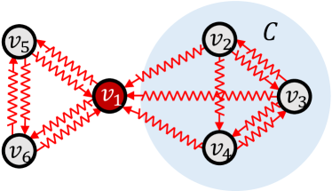
(a)

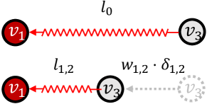
(b)

Figure 3. Spring-like local neighborhood and attractive force.

5. Experiments

In this part, we first elaborate on the experimental settings, and then evaluate the performance of behavior prediction and target recommendation tasks by employing the proposed measures. All of our experiments are conducted on an in-house cluster consisting of hundreds of machines, each of which runs CentOS, and has 16GB memory and 12 Intel Xeon Processor E5-2670 CPU cores.

5.1. Experimental Settings

Datasets. We use 3 friendship-enhancing event datasets from Tencent’s first person shooter (FPS) and multiuser online battle arena (MOBA) games. A given event, whose procedure is explained in Section 2.3, takes the snapshot of $\mathcal{G}$ before the release time as the input graph, since $\mathcal{G}$ for a particular online game evolves when new users are registered, or friendships are modified. We select events FPS and MOBA-A as datasets to evaluate the performance on target adoption and source invitation behavior predictions, and events MOBA-A and MOBA-B to evaluate the performance on target recommendation. The statistics of the graph snapshot, source, and target sets for events are summarized in Table 2. All datasets have been anonymized to avoid any leakage of privacy information.

Competitors. We compare the proposed ${\mathsf{SIT}}$-based measures with 8 representative prior ones as mentioned in Section 2.2: (i) individual-level measures: tie strength (${\mathsf{Tie}}$) (Fang et al., 2014), number of common neighbors (${\mathsf{COM}}$) (Adamic and Adar, 2003), ${\mathsf{PPR}}$ (Page et al., 1999), cosine and euclidean similarity between Node2Vec representations (${\mathsf{N2V}}$(${\mathsf{cos}}$) and ${\mathsf{N2V}}$(${\mathsf{euc}}$)) (Grover and Leskovec, 2016); (ii) group-level measures: structural diversity ($\#$${\mathsf{CC}}$) (Ugander et al., 2012), user-group tie strength (${\mathsf{GT}}$) (Barbieri et al., 2014) and group edge density (${\mathsf{GD}}$) (Purohit et al., 2014). All measures are computed based on the network structure as introduced in Table 2. Notice in Tencent’s MOBA and FPS online gaming platforms that the edge weight between a pair of users is described by the intimacy score, which records the number of historical activities/interactions from one to the other, e.g., co-playing, gifting, etc. For a fair comparison, we employ intimacy values to measure the tie strength for all related ${\mathsf{SIT}}$-based measures and competitors. Furthermore, we employ distributed frameworks in (Lin, 2019) and  (Lin, 2021; Lin et al., 2020) to compute ${\mathsf{PPR}}$ and ${\mathsf{N2V}}$-based measures, respectively, and set the final embedding dimension of the latent vector to 200. To accomplish downstream tasks, we treat our proposal called ${\mathsf{SIT}}$ (including $\#$${\mathsf{CC}}$, ${\mathsf{GS}}$, ${\mathsf{GPR}}$, ${\mathsf{GPPR}}$, ${\mathsf{UGT}}$, and ${\mathsf{IGT}}$) or competing measures as input features for ${\mathsf{XGBoost}}$ as mentioned in Section 3, in which the parameters are set following the original paper (Chen and Guestrin, 2016).

Table 2. Dataset statistics ($\boldsymbol{M\!=\!10^{6},B\!=\!10^{9}}$).

Dataset	$\boldsymbol{|\mathcal{V}|}$	$\boldsymbol{|\mathcal{E}|}$	$\boldsymbol{|\mathcal{S}|}$	$\boldsymbol{|\mathcal{T}|}$
FPS	$77.2M$	$1.1B$	$33.5M$	$43.6M$
MOBA-A	$111.0M$	$4.5B$	$111.0M$	$94.7M$
MOBA-B	$130.2M$	$6.5B$	$120.5M$	$99.7M$

Table 3. Comparison of existing measures and proposed $\boldsymbol{\mathsf{SIT}}$ measure (the best is colored and the second best is underlined).

Measure	Adoption						Invitation
	FPS			MOBA-A			FPS			MOBA-A
	AUC	Accuracy	F1 score	AUC	Accuracy	F1 score	AUC	Accuracy	F1 score	AUC	Accuracy	F1 score
${\mathsf{Tie}}$	0.7154	0.6965	0.6554	0.6017	0.6021	0.3958	0.6072	0.5985	0.4607	0.5361	0.5353	0.2200
${\mathsf{COM}}$	0.5488	0.5538	0.5615	0.5667	0.5576	0.6219	0.5456	0.5323	0.4674	0.5332	0.5281	0.5565
${\mathsf{PPR}}$	0.6565	0.6036	0.5596	0.5562	0.5388	0.4447	0.6289	0.5972	0.5786	0.5846	0.5589	0.5467
${\mathsf{N2V}}$(${\mathsf{cos}}$)	0.6976	0.6610	0.7171	0.5808	0.5626	0.5420	0.5608	0.5537	0.5683	0.5770	0.5630	0.5426
${\mathsf{N2V}}$(${\mathsf{euc}}$)	0.7076	0.6652	0.7091	0.5664	0.5566	0.5390	0.5679	0.5588	0.5628	0.5739	0.5585	0.5375
${\mathsf{GT}}$	0.6985	0.6572	0.6004	0.6295	0.5959	0.5777	0.5738	0.5652	0.3988	0.5397	0.5297	0.4875
${\mathsf{GD}}$	0.6077	0.5736	0.5269	0.6039	0.5728	0.5908	0.5811	0.5507	0.4490	0.5674	0.5508	0.4991
${\mathsf{SIT}}$	0.7995	0.7206	0.7350	0.7410	0.6780	0.6638	0.7307	0.6719	0.6754	0.6550	0.6086	0.6047

Table 4. Comparison of different $\boldsymbol{\mathsf{SIT}}$ variants (the best is colored and the second best is underlined).

Measure	Adoption						Invitation
	FPS			MOBA-A			FPS			MOBA-A
	AUC	Accuracy	F1 score	AUC	Accuracy	F1 score	AUC	Accuracy	F1 score	AUC	Accuracy	F1 score
$\#$${\mathsf{CC}}$	0.6153	0.5897	0.5378	0.5452	0.5288	0.4136	0.6091	0.5820	0.5392	0.5790	0.5551	0.5662
${\mathsf{GS}}$	0.5866	0.5703	0.5323	0.5860	0.5720	0.6182	0.5669	0.5448	0.4827	0.5655	0.5510	0.5266
${\mathsf{GPR}}$	0.6509	0.6071	0.6150	0.6567	0.6149	0.6403	0.6817	0.6314	0.6325	0.6382	0.5978	0.6044
-sum	0.5750	0.5538	0.5702	0.5651	0.5469	0.5798	0.6074	0.5699	0.4978	0.5783	0.5531	0.5545
${\mathsf{GPPR}}$	0.6337	0.5990	0.5630	0.5641	0.5405	0.4433	0.6258	0.5922	0.5747	0.5895	0.5603	0.5902
-sum	0.6230	0.5727	0.5749	0.5874	0.5671	0.6217	0.5771	0.5472	0.5634	0.5683	0.5493	0.5545
${\mathsf{UGT}}$	0.7427	0.6965	0.7249	0.5634	0.5482	0.5061	0.5969	0.5772	0.5793	0.5684	0.5525	0.5345
-euc	0.7233	0.6857	0.7266	0.5492	0.5345	0.5199	0.5844	0.5643	0.5761	0.5650	0.5505	0.5402
-sum	0.7374	0.6621	0.6145	0.6380	0.6035	0.5793	0.5920	0.5695	0.4477	0.5574	0.5378	0.5695
${\mathsf{IGT}}$	0.5622	0.5425	0.4388	0.6296	0.6047	0.5487	0.5372	0.5236	0.3694	0.5642	0.5496	0.4616
-euc	0.5645	0.5650	0.4670	0.5733	0.5569	0.6265	0.5344	0.5239	0.3617	0.5681	0.5521	0.4660
-sum	0.5638	0.5560	0.5008	0.5915	0.5708	0.6058	0.5620	0.5373	0.4605	0.5705	0.5531	0.5170
$\#$${\mathsf{CC}}$-${\mathsf{GS}}$	0.6698	0.6180	0.6038	0.6101	0.5857	0.6252	0.6306	0.5978	0.5808	0.5972	0.5665	0.5550
${\mathsf{SIT}}$	0.7995	0.7206	0.7350	0.7410	0.6780	0.6638	0.7307	0.6719	0.6754	0.6550	0.6086	0.6047

5.2. Behavior Prediction

In this section, we separately train two sets of ${\mathsf{XGBoost}}$ models to evaluate the performance of the aforementioned methods in predicting target adoption and source invitation behaviors. Notice that user behaviors can be interfered with by the underlying exposure strategies, which will be illustrated in Section 5.3. To eliminate the bias, we focus on randomly exposed source-target pairs, in which we select the pairs with invitation or adoption behaviors as positive data instances and also randomly select an equal number of pairs without behaviors as negative data instances (Zhang et al., 2021). Finally, we obtain 116.3 (resp. 12.5) thousands of data instances for invitation (resp. adoption) prediction on FPS, and 776.4 (resp. 39.1) thousands of instances for invitation (resp. adoption) prediction on MOBA-A, where 80% are used for training and 20% for testing. To evaluate the effectiveness, we repeat each approach 3 times and report the average result under conventional metrics: Area Under Curve (AUC), accuracy and F1 score. In the following experiments, we compare our proposal called ${\mathsf{SIT}}$ with each competitor, every single dimension of ${\mathsf{SIT}}$ and their variants in order, followed by analyzing each ${\mathsf{SIT}}$ dimension. Note that we first show the results about target adoptions and then those about source invitations, as the primary goal of ${\mathsf{SIT}}$ to understand how targets are influenced.

Overall Performance. As illustrated in Table 3, our proposed ${\mathsf{SIT}}$ consistently outperforms other competitors in both FPS and MOBA-A datasets. Specifically, while predicting target adoption behaviors, ${\mathsf{SIT}}$ is 11.8%, 3.5%, 2.5% (resp. 23.2% 12.6% 6.7%) better than the best competitor in terms of AUC, accuracy, and F1 score in FPS (resp. MOBA-A). For invitation behaviors, ${\mathsf{SIT}}$ is 16.2%, 12.3%, 16.7% (resp. 12.0%, 8.1%, and 8.7%) better than the best competitor in terms of AUC, accuracy, and F1 score in FPS (resp. MOBA-A). The above results reflect that involving group information by ${\mathsf{SIT}}$ is necessary for understanding user behaviors in friendship-enhancing events. Regarding competitors, ${\mathsf{Tie}}$ is the best-performing competitor in terms of AUC and accuracy scores during the adoption prediction, which indicates that source-target pairs with more historical interactions (i.e., intimacy) are more likely to interact again. Correspondingly, AUC and accuracy scores of ${\mathsf{GT}}$ and ${\mathsf{GD}}$ are also comparable due to the usage of intimacy values. Furthermore, the F1 score of other single-level measures (${\mathsf{PPR}}$, ${\mathsf{COM}}$ or ${\mathsf{N2V}}$(${\mathsf{cos}}$)) is the second best on both datasets w.r.t. adoption and invitation predictions. Regarding the structural diversity ($\#$${\mathsf{CC}}$), we evaluate its performance in the ablation study, as it is a dimension of ${\mathsf{SIT}}$.

Ablation study. As illustrated in Table 4, we find that each dimension i.e., $\#$${\mathsf{CC}}$, ${\mathsf{GS}}$, ${\mathsf{GPR}}$, ${\mathsf{GPPR}}$, ${\mathsf{UGT}}$, or ${\mathsf{IGT}}$, is less effective than ${\mathsf{SIT}}$. For both behaviors and datasets, ${\mathsf{UGT}}$ or ${\mathsf{GPR}}$ performs as the best competitor in all evaluation metrics, compared with both other ${\mathsf{SIT}}$-based dimensions and all competitors in Table 3. Regarding ${\mathsf{IGT}}$, it is less effective than ${\mathsf{UGT}}$ and ${\mathsf{GPR}}$, but is still comparable to the existing measures in Table 3. For instance, the ${\mathsf{IGT}}$ score is 4.3%, 5.6% better than the group-level competitor ${\mathsf{GD}}$ in terms of AUC and accuracy for adoption behaviors of MOBA-A, as ${\mathsf{IGT}}$ additionally involves the similarities among in-group members. Notice that both $\#$${\mathsf{CC}}$ and ${\mathsf{GS}}$ scores are analyzed in the work of structural diversity (Ugander et al., 2012) and can be treated as competitors of other ${\mathsf{SIT}}$-based measures. In particular, we assemble both measures into ${\mathsf{XGBoost}}$ and denote the model instance as $\#$${\mathsf{CC}}$-${\mathsf{GS}}$, whose scores can extensively outperform those of each single measure $\#$${\mathsf{CC}}$ and ${\mathsf{GS}}$ as reported in Table 4. However, $\#$${\mathsf{CC}}$-${\mathsf{GS}}$ are still worse than some single dimensions (i.e., ${\mathsf{GPR}}$ or ${\mathsf{UGT}}$) and the proposed ${\mathsf{SIT}}$. Regarding the reasons for the performance of each dimension in ${\mathsf{SIT}}$, we leave them in the analysis parts.

(a)

(b)

(c)

(d)

(e)

(f)

Figure 4. Conversion probability of adoption behaviors conditioned on each $\boldsymbol{\mathsf{SIT}}$-based measure in FPS.

(a)

(b)

(c)

(d)

(e)

(f)

Figure 5. Conversion probability of invitation behaviors conditioned on each $\boldsymbol{\mathsf{SIT}}$-based measure in FPS.

Factor formulation. As mentioned in Section 4, other possible formulations of proposed measures exist. Thus, except for the averaged aggregation operation and cosine similarity, we also evaluate the performance of variant measures with summation operation and euclidean similarity (denoted as sum and euc, respectively) in Table 4. To derive the euclidean similarity, we first normalize the euclidean distance between each node pair by the min-max scaler as the cosine similarity does, and then take the one minus normalized distance as the corresponding similarity. In particular, employing the summation operation is equivalent to hybrid the original measure with the factor of ${\mathsf{GS}}$, which may dampen the original measure (i.e., ${\mathsf{GPR}}$, ${\mathsf{GPPR}}$, ${\mathsf{UGT}}$ or ${\mathsf{IGT}}$) because of the weak correlation between ${\mathsf{GS}}$ and user behaviors, which will be shown in Figures 4-5. For example, the result quality of the summation of ${\mathsf{GPR}}$ is consistently worse than that of ${\mathsf{GPR}}$ on both behaviors and datasets. As for different similarity measures w.r.t node representations, the effectiveness of utilizing cosine and euclidean similarity is comparable. In particular, the F1 scores of euclidean-based ${\mathsf{UGT}}$ and ${\mathsf{IGT}}$ are usually better than those of cosine-based. Meanwhile, negative results are reported regarding AUC and accuracy scores.

Conversion probability conditioned on $\boldsymbol{\mathsf{SIT}}$ dimensions. We investigate the relation between user behaviors and the aforementioned ${\mathsf{SIT}}$-based measures: $\#$${\mathsf{CC}}$, ${\mathsf{GS}}$, ${\mathsf{GPR}}$, ${\mathsf{GPPR}}$, ${\mathsf{UGT}}$, and ${\mathsf{IGT}}$. Due to space limitations, we only report the analysis results on FPS, and the rest datasets derive similar results. Following the setting of (Fang et al., 2014), we employ the density-based discretization to convert the scores of ${\mathsf{SIT}}$-based measures into five different levels, where a higher level indicates a larger score. Moreover, we use conversion probability (Fang et al., 2014; Ugander et al., 2012) to evaluate how the user acts. In particular, given a level of certain ${\mathsf{SIT}}$ measure, the adoption (resp. invitation) conversion probability is the fraction of source-target pairs existing adoption (resp. invitation) behaviors over all pairs in this level.

We report the adoption and invitation conversion probabilities w.r.t each measure in Figure 4 and Figure 5, respectively. We can find an evident correlation between each behavior and each proposed measure except for ${\mathsf{GS}}$. In terms of $\#$${\mathsf{CC}}$, contradicting the well-accepted insight of structural diversity (Ugander et al., 2012; Su et al., 2020; Fang et al., 2014), Figures 4(a) and  5(a) show that the target user with less number of candidate groups (i.e., a less diverse neighborhood) is more likely to be invited and further adopt this invitation. Recently, this phenomenon also emerged from other user behaviors, especially in Tencent instant messaging platform (Qiu et al., 2016; Zhang et al., 2021), but the underlying reason is still unclear. In contrast, ${\mathsf{SIT}}$ can explain this as that a greater multi-membership makes the social identification phase of a target challenging due to the potential role conflict (Marks, 1977). Regarding the effect of group size, we can find in Figures 4(b) and  5(b) that the engagement willingness of users will be facilitated as the group scale increases, but subsequently hurdled if still going up. Notice that the source-target pair inside a medium-size group (i.e., level 3) is more likely to send an invitation and respond.

Recall in Section 4 that ${\mathsf{GPR}}$ and ${\mathsf{GPPR}}$ measure the factors of social standing and centrality from the global and personalized view, respectively. The results in Figures 4(d) and 5(d) show that the target user is more likely to choose a relatively important group, which confirms the claim of the centrality factor in ${\mathsf{SIT}}$. However, Figures 4(c) and 5(c) illustrate opposing results w.r.t ${\mathsf{GPR}}$. The reason is that, by definition, a user with a high PageRank value tends to have more neighbors, which consequently means each target friend has less probability of being exposed by the random algorithm.

To evaluate the tie strength and similarity parts in ${\mathsf{UGT}}$, we separate them as ${\mathsf{UGT}}$-$w$ and ${\mathsf{UGT}}$-$\delta$ respectively, in which ${\mathsf{UGT}}$-$w$ measures the averaged intimacy values and ${\mathsf{UGT}}$-$\delta$ measures the averaged cosine similarity between the Node2Vec representations. The same operation is also performed for ${\mathsf{IGT}}$. As illustrated in Figures 4(e) and 5(e), the behavior conversion probabilities increase as the levels of ${\mathsf{UGT}}$-$w$ and ${\mathsf{UGT}}$-$\delta$ go up, which match the factors of solidarity and self-stereotyping in ${\mathsf{SIT}}$. The same tendency for ${\mathsf{IGT}}$ is shown in Figures 4(f) and 5(f). However, the correlation regarding ${\mathsf{IGT}}$ is relatively weak as it fails to provide intra-group information for the group with only one member.

Table 5. $\boldsymbol{\mathsf{SIT}}$ feature importance w.r.t adoption behavior.

	$\#$${\mathsf{CC}}$	${\mathsf{GS}}$	${\mathsf{GPR}}$	${\mathsf{GPPR}}$	${\mathsf{UGT}}$	${\mathsf{IGT}}$
FPS	0.1413	0.1179	0.2291	0.1713	0.2191	0.1212
MOBA-A	0.1561	0.1345	0.1958	0.1733	0.2139	0.1264

Table 6. $\boldsymbol{\mathsf{SIT}}$ feature importance w.r.t invitation behavior.

	$\#$${\mathsf{CC}}$	${\mathsf{GS}}$	${\mathsf{GPR}}$	${\mathsf{GPPR}}$	${\mathsf{UGT}}$	${\mathsf{IGT}}$
FPS	0.1404	0.0809	0.2081	0.2221	0.2271	0.1214
MOBA-A	0.1522	0.1002	0.2540	0.1819	0.1907	0.1210

Importance of $\boldsymbol{\mathsf{SIT}}$ dimensions. ${\mathsf{XGBoost}}$ supports measuring the importance of each input feature, where the importance indicates the frequency that a feature is leveraged to split the data across all trees. Table 5 and Table 6 report the feature importance of each proposed ${\mathsf{SIT}}$-based measure w.r.t adoption and invitation behaviors, respectively. In particular, ${\mathsf{GPR}}$, ${\mathsf{GPPR}}$, and ${\mathsf{UGT}}$ have the top-3 highest importance w.r.t both behaviors, which indicates that social standing, centrality, solidarity, and self-stereotyping are more critical ${\mathsf{SIT}}$ factors. As for ${\mathsf{GS}}$ and ${\mathsf{IGT}}$, they perform as the bottom-2 important features. This is because they are less correlated with user behaviors, as illustrated in Figures 4-5. In contrast, $\#$${\mathsf{CC}}$ is also less important even though it has quite strong correlation to user behaviors. This is due to that $\#$${\mathsf{CC}}$ is a stand-alone measure for the target user and hence incurs indistinguishable values for source-target pairs with the same target user. To summarize, the aforementioned results of the correlation and importance analysis can explain each ${\mathsf{SIT}}$ dimension’s performance in Table 4.

5.3. Target Recommendation

Deployment setups. Recall in Section 2.3 that a source user can only select the target users from a feed window of limited size $k$ during the second step of a friendship-enhancing event. Therefore, judiciously exposing a subset of target friends for the source $v_{i}$ is pivotal to the event’s performance. Motivated by this, the target recommendation task (Problem 2) is to find $k$ target users w.r.t the source to boost the overall engagement of sources and targets. Here, we inherit the ${\mathsf{XGBoost}}$ model, which takes the aforementioned individual measures (i.e., ${\mathsf{Tie}}$ (measured by intimacy), ${\mathsf{COM}}$, ${\mathsf{PPR}}$, and ${\mathsf{N2V}}$(${\mathsf{euc}}$)) or ${\mathsf{SIT}}$ measures as the input and is trained based on the historical events. We sort the predicted value $\hat{y}_{i,j}$ w.r.t each source $v_{i}$ in a descending order and select the top-$k$ target nodes to recommend. To evaluate the proposed ${\mathsf{SIT}}$ measures, we conduct the online A/B testing that randomly assigns a fraction of live traffic to ${\mathsf{XGBoost}}$ models with individual-level measures as treatment groups. Initially, each measure is computed based on the graph instance ahead of the event (see Table 2). Afterward, each measure is updated daily by using the latest graph snapshot.

Table 7. Online performance in MOBA-A.

Measure	${\mathsf{Tie}}$	${\mathsf{COM}}$	${\mathsf{PPR}}$	${\mathsf{N2V}}$(${\mathsf{euc}}$)	${\mathsf{SIT}}$
E2E rate	0.1018	0.0958	0.1066	0.0739	0.1431

Table 8. Online performance in MOBA-B.

Measure	${\mathsf{Tie}}$	${\mathsf{PPR}}$	${\mathsf{SIT}}$
E2E rate	0.1152	0.1218	0.1384

Overall performance. We evaluate the effectiveness of different online random trials by the end-to-end (E2E) rate, which considers the overall engagement of sources and targets. In particular, E2E rate equals the fraction of target friends adopting the invitations over the source users seeing the event. The higher E2E rate indicates better quality. As illustrated in Table 7, the proposed solution ${\mathsf{SIT}}$ has the highest E2E rate on MOBA-A. Specifically, ${\mathsf{SIT}}$ is 34.2% better than the best-performed treatment approach ${\mathsf{PPR}}$. Furthermore, we can find that ${\mathsf{PPR}}$ and ${\mathsf{Tie}}$ can outperform the other two competitors. Motivated by this, we conduct another online trial on MOBA-B by comparing ${\mathsf{SIT}}$ with the best two measures ${\mathsf{PPR}}$ and ${\mathsf{Tie}}$. Specifically, Table 8 reports that ${\mathsf{SIT}}$ is 13.6% better than the best-performed treatment approach ${\mathsf{PPR}}$.

6. Additional Related Works

This part briefly reviews other ${\mathtt{TFC}}$ measures and the related sociological theory. In particular, prior ${\mathtt{TFC}}$ measures can be explained by either selection or influence mechanism in the homophily principle (Easley et al., 2010). The selection indicates that people tend to form friendships with others with similar characteristics. In contrast, the influence can be treated as the inverse of selection, claiming that people may modify characteristics to conform to their friends. We categorize ${\mathtt{TFC}}$ measures based on the taxonomy of selection and influence.

Regarding the selection, conventional ${\mathtt{TFC}}$ measures utilize the variant based on common neighborhood, e.g., Adamic/Adar score (Adamic and Adar, 2003). Furthermore, the selection can be measured by the similarity between node embeddings, e.g., (Roweis and Saul, 2000; Tang et al., 2015; Wang et al., 2016; Perozzi et al., 2014; Grover and Leskovec, 2016; Yang et al., 2020), which essentially rely on the factorization of a matrix of the ${\mathtt{TFC}}$ measure as mentioned in Section 2.2 (Qiu et al., 2018). Regarding social influence, the related measures mainly focus on the local structure of a user. Burt (Burt, 1987) proposes to model social influence from cohesion and structural equivalence perspectives. In particular, cohesion describes the direct influence measured by tie strength and the number of influenced friends (Granovetter, 1978; Fang et al., 2014). The structural equivalence describes the indirect influence between users and is measured by tie embeddedness (Easley et al., 2010). Recently, many learning-based methods (Gomez-Rodriguez et al., 2011; Sankar et al., 2020; Li et al., 2020) are proposed to predict the influence probability based on historical cascades, among which (Li et al., 2020) leverages another psychological concept called conformity to measure the social influence.

In contrast, ${\mathsf{SIT}}$ is a group-level psychological framework, in which each dimension can reflect either selection or influence in the homophily principle. For instance, the factors of self-stereotyping and in-group homogeneity are coherent with the selection mechanism. Therefore, ${\mathsf{SIT}}$ can also provide theoretical support for the aforementioned measures and their integration, e.g., (Sankar et al., 2020).

7. Conclusions

In this work, we propose measures for friendship closeness based on the social identity theory, a fundamental concept in social psychology, and conduct extensive experiments and analysis on 3 Tencent’s online gaming datasets. Compared with 8 state-of-the-art methods, our proposal achieves the highest effectiveness on both behavior prediction and target recommendation tasks. Regarding future works, we will employ presented measures for other scenarios, e.g., modeling the cascade of social influence and suggesting strangers to enrich users’ friendships in the who-to-follow service.

- (1)
- Adamic and Adar (2003) Lada A Adamic and Eytan Adar. 2003. Friends and neighbors on the web. Social networks 25, 3 (2003), 211–230.
- Barbieri et al. (2014) Nicola Barbieri, Francesco Bonchi, and Giuseppe Manco. 2014. Who to follow and why: link prediction with explanations. In SIGKDD. 1266–1275.
- Brewer and Gardner (1996) Marilynn B Brewer and Wendi Gardner. 1996. Who is this” We”? Levels of collective identity and self representations. Journal of personality and social psychology 71, 1 (1996), 83.
- Burt (1987) Ronald S Burt. 1987. Social contagion and innovation: Cohesion versus structural equivalence. American journal of Sociology 92, 6 (1987), 1287–1335.
- Cai et al. (2018) Hongyun Cai, Vincent W Zheng, and Kevin Chen-Chuan Chang. 2018. A comprehensive survey of graph embedding: Problems, techniques, and applications. TKDE 30, 9 (2018), 1616–1637.
- Cameron (2004) James E Cameron. 2004. A three-factor model of social identity. Self and identity 3, 3 (2004), 239–262.
- Chen and Guestrin (2016) Tianqi Chen and Carlos Guestrin. 2016. Xgboost: A scalable tree boosting system. In SIGKDD. 785–794.
- De et al. (2016) Abir De, Sourangshu Bhattacharya, Sourav Sarkar, Niloy Ganguly, and Soumen Chakrabarti. 2016. Discriminative link prediction using local, community, and global signals. TKDE 28, 8 (2016), 2057–2070.
- Doosje et al. (1998) Bertjan Doosje, Nyla R Branscombe, Russell Spears, and Antony SR Manstead. 1998. Guilty by association: When one’s group has a negative history. Journal of personality and social psychology 75, 4 (1998), 872.
- Easley et al. (2010) David Easley, Jon Kleinberg, et al. 2010. Networks, crowds, and markets. Vol. 8. Cambridge university press Cambridge.
- Epasto et al. (2015) Alessandro Epasto, Silvio Lattanzi, Vahab Mirrokni, Ismail Oner Sebe, Ahmed Taei, and Sunita Verma. 2015. Ego-net community mining applied to friend suggestion. PVLDB 9, 4 (2015), 324–335.
- Everett and Borgatti (1999) Martin G Everett and Stephen P Borgatti. 1999. The centrality of groups and classes. The Journal of mathematical sociology 23, 3 (1999), 181–201.
- Fang et al. (2014) Zhanpeng Fang, Xinyu Zhou, Jie Tang, Wei Shao, Alvis Cheuk M Fong, Longjun Sun, Ying Ding, Ling Zhou, and Jarder Luo. 2014. Modeling paying behavior in game social networks. In CIKM. 411–420.
- Fruchterman and Reingold (1991) Thomas MJ Fruchterman and Edward M Reingold. 1991. Graph drawing by force-directed placement. SP&E 21, 11 (1991), 1129–1164.
- Gaertner and Dovidio (2014) Samuel L Gaertner and John F Dovidio. 2014. Reducing intergroup bias: The common ingroup identity model. Psychology Press.
- Gansner et al. (2004) Emden R Gansner, Yehuda Koren, and Stephen North. 2004. Graph drawing by stress majorization. In GD. 239–250.
- Gomez-Rodriguez et al. (2011) Manuel Gomez-Rodriguez, David Balduzzi, and Bernhard Schölkopf. 2011. Uncovering the temporal dynamics of diffusion networks. In ICML.
- Granovetter (1978) Mark Granovetter. 1978. Threshold models of collective behavior. American journal of sociology (1978).
- Grover and Leskovec (2016) Aditya Grover and Jure Leskovec. 2016. node2vec: Scalable feature learning for networks. In SIGKDD. 855–864.
- Jeh and Widom (2002) Glen Jeh and Jennifer Widom. 2002. Simrank: a measure of structural-context similarity. In SIGKDD. 538–543.
- Leach et al. (2008) Colin Wayne Leach, Martijn Van Zomeren, Sven Zebel, Michael LW Vliek, Sjoerd F Pennekamp, Bertjan Doosje, Jaap W Ouwerkerk, and Russell Spears. 2008. Group-level self-definition and self-investment: a hierarchical (multicomponent) model of in-group identification. Journal of personality and social psychology 95, 1 (2008), 144.
- Li et al. (2020) Hui Li, Hui Li, and Sourav S Bhowmick. 2020. Chassis: Conformity meets online information diffusion. In SIGMOD. 1829–1840.
- Lin (2019) Wenqing Lin. 2019. Distributed algorithms for fully personalized pagerank on large graphs. In TheWebConf. 1084–1094.
- Lin (2021) Wenqing Lin. 2021. Large-Scale Network Embedding in Apache Spark. In SIGKDD. 3271–3279.
- Lin et al. (2020) Wenqing Lin, Feng He, Faqiang Zhang, Xu Cheng, and Hongyun Cai. 2020. Initialization for Network Embedding: A Graph Partition Approach. In WSDM. 367–374.
- Luo et al. (2019) Siqiang Luo, Xiaokui Xiao, Wenqing Lin, and Ben Kao. 2019. Efficient batch one-hop personalized pageranks. In ICDE. 1562–1565.
- Luo et al. (2020) Siqiang Luo, Xiaokui Xiao, Wenqing Lin, and Ben Kao. 2020. BATON: Batch One-Hop Personalized PageRanks with Efficiency and Accuracy. IEEE Trans. Knowl. Data Eng. 32, 10 (2020), 1897–1908.
- Marks (1977) Stephen R Marks. 1977. Multiple roles and role strain: Some notes on human energy, time and commitment. American sociological review (1977), 921–936.
- Oakes et al. (1994) Penelope J Oakes, S Alexander Haslam, and John C Turner. 1994. Stereotyping and social reality. Blackwell Publishing.
- Page et al. (1999) Lawrence Page, Sergey Brin, Rajeev Motwani, and Terry Winograd. 1999. The PageRank citation ranking: Bringing order to the web. Technical Report. Stanford InfoLab.
- Perozzi et al. (2014) Bryan Perozzi, Rami Al-Rfou, and Steven Skiena. 2014. Deepwalk: Online learning of social representations. In SIGKDD. 701–710.
- Purohit et al. (2014) Hemant Purohit, Yiye Ruan, David Fuhry, Srinivasan Parthasarathy, and Amit Sheth. 2014. On understanding the divergence of online social group discussion. In ICWSM, Vol. 8. 396–405.
- Qiu et al. (2018) Jiezhong Qiu, Yuxiao Dong, Hao Ma, Jian Li, Kuansan Wang, and Jie Tang. 2018. Network embedding as matrix factorization: Unifying deepwalk, line, pte, and node2vec. In WSDM. 459–467.
- Qiu et al. (2016) Jiezhong Qiu, Yixuan Li, Jie Tang, Zheng Lu, Hao Ye, Bo Chen, Qiang Yang, and John E Hopcroft. 2016. The lifecycle and cascade of wechat social messaging groups. In TheWebConf. 311–320.
- Rees et al. (2015) Tim Rees, S Alexander Haslam, Pete Coffee, and David Lavallee. 2015. A social identity approach to sport psychology: Principles, practice, and prospects. Sports medicine 45, 8 (2015), 1083–1096.
- Roweis and Saul (2000) Sam T Roweis and Lawrence K Saul. 2000. Nonlinear dimensionality reduction by locally linear embedding. Science 290, 5500 (2000), 2323–2326.
- Sankar et al. (2020) Aravind Sankar, Xinyang Zhang, Adit Krishnan, and Jiawei Han. 2020. Inf-vae: A variational autoencoder framework to integrate homophily and influence in diffusion prediction. In WSDM. 510–518.
- Scheepers and Ellemers (2019) Daan Scheepers and Naomi Ellemers. 2019. Social identity theory. In Social psychology in action. 129–143.
- Seering et al. (2018) Joseph Seering, Felicia Ng, Zheng Yao, and Geoff Kaufman. 2018. Applications of social identity theory to research and design in computer-supported cooperative work. PCHI 2, CSCW (2018), 1–34.
- Shu et al. (2017) Kai Shu, Amy Sliva, Suhang Wang, Jiliang Tang, and Huan Liu. 2017. Fake news detection on social media: A data mining perspective. SIGKDD 19, 1 (2017), 22–36.
- Sieber (1974) Sam D Sieber. 1974. Toward a theory of role accumulation. American sociological review (1974), 567–578.
- Simon (1992) Bernd Simon. 1992. The perception of ingroup and outgroup homogeneity: Reintroducing the intergroup context. European review of social psychology 3, 1 (1992), 1–30.
- Song et al. (2020) Junho Song, Hyekyoung Park, Kyungsik Han, and Sang-Wook Kim. 2020. Do You Really Like Her Post?: Network-Based Analysis for Understanding Like Activities in SNS. In CIKM. 2221–2224.
- Song et al. (2007) Xiaodan Song, Yun Chi, Koji Hino, and Belle Tseng. 2007. Identifying opinion leaders in the blogosphere. In CIKM. 971–974.
- Soundarajan and Hopcroft (2012) Sucheta Soundarajan and John Hopcroft. 2012. Using community information to improve the precision of link prediction methods. In WWW. 607–608.
- Su et al. (2020) Jessica Su, Krishna Kamath, Aneesh Sharma, Johan Ugander, and Sharad Goel. 2020. An experimental study of structural diversity in social networks. In ICWSM, Vol. 14. 661–670.
- Tajfel and Turner (2004) Henri Tajfel and John C Turner. 2004. The social identity theory of intergroup behavior. In Political psychology. 276–293.
- Tang et al. (2015) Jian Tang, Meng Qu, Mingzhe Wang, Ming Zhang, Jun Yan, and Qiaozhu Mei. 2015. Line: Large-scale information network embedding. In TheWebConf. 1067–1077.
- Tong et al. (2006) Hanghang Tong, Christos Faloutsos, and Jia-Yu Pan. 2006. Fast random walk with restart and its applications. In ICDM. 613–622.
- Ugander et al. (2012) Johan Ugander, Lars Backstrom, Cameron Marlow, and Jon Kleinberg. 2012. Structural diversity in social contagion. PNAS 109, 16 (2012), 5962–5966.
- Wang et al. (2016) Daixin Wang, Peng Cui, and Wenwu Zhu. 2016. Structural deep network embedding. In SIGKDD. 1225–1234.
- Wu et al. (2016) Liang Wu, Xia Hu, and Huan Liu. 2016. Relational learning with social status analysis. In WSDM. 513–522.
- Yang and Leskovec (2015) Jaewon Yang and Jure Leskovec. 2015. Defining and evaluating network communities based on ground-truth. KIS 42, 1 (2015), 181–213.
- Yang et al. (2020) Renchi Yang, Jieming Shi, Xiaokui Xiao, Yin Yang, and Sourav S Bhowmick. 2020. Homogeneous Network Embedding for Massive Graphs via Reweighted Personalized PageRank. PVLDB 13, 5 (2020).
- Zhang et al. (2021) Fanjin Zhang, Jie Tang, Xueyi Liu, Zhenyu Hou, Yuxiao Dong, Jing Zhang, Xiao Liu, Ruobing Xie, Kai Zhuang, Xu Zhang, et al. 2021. Understanding WeChat User Preferences and “Wow” Diffusion. TKDE 1 (2021), 1–1.
- Zhang et al. (2018) Yuanxing Zhang, Zhuqi Li, Chengliang Gao, Kaigui Bian, Lingyang Song, Shaoling Dong, and Xiaoming Li. 2018. Mobile social big data: Wechat moments dataset, network applications, and opportunities. IEEE network 32, 3 (2018), 146–153.