Precise Evolutionary Asteroseismology of High-Amplitude $\delta$ Scuti Star AE Ursae Majoris

Abstract

Stellar structure and evolution theory is one of the basis in modern astronomy. Stellar inner structures and their evolutionary states can be precisely tested by asteroseismology, since the inner information is brought to the stellar surface by the global oscillating waves and becomes observable. For stellar evolutionary speed (i.e. how long time scale does a star stay at a special evolution phase?), because of the insurmountable gap between the time scales of the evolutionary history of human civilization and a star, it can only be roughly tested by ensemble of stars in different evolutionary stages in most cases, and all the snapshots of these stars make up our global view of stellar evolution. The effect of stellar evolution on the structure and the corresponding global size of a pulsating star will lead to tiny period variations of its pulsation modes, which are the most valuable indicators of its evolutionary state and can be used to test the stellar evolution theory by a single star rather than ensemble of stars. Here, we report a High-Amplitude $\delta$ Scuti star AE Ursae Majoris, who locates in the post main-sequence (MS) evolutionary stage and its observed linear period variation rate can be practically ascribed to its evolutionary effect. The result tests the stellar evolution theory from the pre-MS to post-MS with an unprecedented precision by a single star, and the framework can be extended to other type of pulsating stars to perform precise evolutionary asteroseismology, which aims to test the current stellar evolution theory in different evolutionary stages, discover the discrepancies between the theory and observations, and ultimately build a complete and precise stellar evolution theory to backtrack the history of each of these stars.

1 Introduction

$\delta$ Scuti stars are a kind of short-period pulsating variable stars whose periods range from 15 minutes to 8 hours and the spectral classes A-F. They locate on the main sequence (MS) or post-MS evolutionary stage at the bottom of the classical Cepheid instability strip in Hertzsprung-Russell diagram (H-R diagram) and are self-excited by the kappa mechanism due to the partial ionization of helium in the out layers (Breger, 2000; Handler, 2009; Uytterhoeven et al., 2011; Holdsworth et al., 2014). High-amplitude $\delta$ Scuti stars (hereafter HADS) are a kind of $\delta$ Scuti stars, who have relatively larger amplitudes ($\Delta V\geq 0_{\cdot}^{m}3$) and slower rotations in most cases. Most of HADS show single or double radial pulsation modes, and some of them have three radial pulsation modes or even some non-radial pulsation modes (Niu et al., 2013, 2017; Xue et al., 2018; Wils et al., 2008; Xue & Niu, 2020; Daszyńska-Daszkiewicz et al., 2022).

Limited by the precision of ground-based photometric observations, only the linear period variation rates of the pulsation modes with the highest amplitudes (usually the fundamental modes) of HADS can be obtained by the accumulation of the data lasting for decades (Yang et al., 2012; Niu et al., 2017; Xue et al., 2018). The high-precision continues photometric observations from spacecraft like Kepler (lasting for four years) can also lead us to get the linear period variation rates of HADS, not only for the highest amplitude pulsation modes, but also for other pulsation modes with sufficient signal-to-noise ratio (Bowman et al., 2016; Niu & Xue, 2021; Bowman et al., 2021). These linear period variation rates ($(1/P)(\,\mathrm{d}P/\,\mathrm{d}t)$) generally have values $\pm(10^{-9}-10^{-6})\,\mathrm{yr}^{-1}$. On the aspect of stellar evolution theory, HADS are always considered to locate in the main-sequence (MS) or post-MS evolutionary stages. In these stages, the linear period variation rates caused by the stellar evolution cannot exceed $20\cdot 10^{-8}\ yr^{-1}$ (Breger & Pamyatnykh, 1998), which are systematically smaller than the observed values and indicate that there exist additional mechanisms (such as mass transfer, light traveling time effect in multiple system, and nonlinear mode interactions) contributing to the linear period variation rates (Breger & Pamyatnykh, 1998; Bowman et al., 2016, 2021; Xue & Niu, 2020). However, some recent researches (Niu et al., 2017; Xue et al., 2018) show that the observed linear period variation rates of some HADS can be roughly included in their asteroseismological models self-consistently.

Whether the observed linear period variation rates of HADS (at least in some individual cases) can be fully predicted by the stellar evolution theory is directly related to two important issues: (i) the physical essence of HADS: the low-amplitude $\delta$ Scuti stars (LADS) always have similar pulsation periods and seem to have almost the same basic physical properties (such as the effective temperature, the luminosity and the surface gravitational acceleration) as HADS, but they have obvious different light curve features. What’s the origin of the difference? If it comes from the different stellar evolution stages (Petersen & Christensen-Dalsgaard, 1996), one should precisely determine the evolutionary stages of them in the framework of current stellar evolution theory, which requires at least the consistency of the observed linear period variation rates and the stellar evolution theory predictions. (ii) the stellar evolution theory: because of the insurmountable gap between the time scales of the evolutionary history of human civilization and stars, the stellar evolution theory is generally constructed, tested, and updated by ensemble of stars in different evolutionary stages base on a statistical sense. The comparison of the linear period variation rates between observations and theoretical predictions of pulsating stars in a rapidly evolving stage (such as HADS) provides us an opportunity to test the current stellar evolution theory by single stars precisely. The deviations between them are the indicators of the self-consistency of the stellar structure and evolution theory to some extend, which would be the important hints to update the current theory in future.

AE Ursae Majoris (hereafter AE UMa, $\alpha_{2000}={09^{h}}{36^{m}}{53^{s}}$, $\delta_{2000}=44^{\circ}04^{\prime}01^{\prime\prime}$, V=11.27 mag) is a Population I, post-MS HADS pulsating in radial modes (Hintz et al., 1997; Pócs & Szeidl, 2001; Zhou, 2001; Niu et al., 2017). Based on the detected frequencies of the fundamental and first overtone pulsation modes ($f_{0}=11.6256\ \,\mathrm{c}\ \mathrm{d}^{-1}$, $f_{1}=15.0312\ \,\mathrm{c}\ \mathrm{d}^{-1}$), together with the linear period variation rate of the fundamental pulsation mode ($\,(1/P_{0})(\,\mathrm{d}P_{0}/\,\mathrm{d}t)=(5.4\pm 1.9)\times 10^{-9}\ \,\mathrm{yr}^{-1}$), Niu et al. (2017) has made a pioneering attempt to do asteroseismology for AE UMa. It shows that AE UMa could be a normal star evolving into the post-MS stage, although the pulsating frequencies obtained from the ground-based telescopes have relatively large uncertainties and the final results have obvious deviations comparing with the observed spectroscopic parameters.

These years, AE UMa has been monitored not only by the Transiting Exoplanet Survey Satellite (TESS (Ricker et al., 2015)), but also by some other ground-based observations whose data have been collected by AAVSO. The continues photometric data from TESS provide us accurate pulsating frequencies, and all the extended data accumulate the number of the times of maximum light (TML), which are necessary for determining a reliable value of the observed linear period variation rate of the fundamental pulsation mode.

2 Methods

2.1 Frequency Analysis

AE UMa (TIC 357132618) has been observed by TESS spacecraft during Sector 21 from 2020 January 21 to 2020 February 18 (BJD 2458870.45 - 2458897.78), in which there exists a gap of about 4 days (see in Figure 1). We downloaded the 2-min cadence flux measurements from MAST Portal which were processed by the TESS Science Processing Operations Center (SPOC; Jenkins et al. (2016)). After converting the normalized fluxes to magnitudes by utilizing a TESS magnitude of +11.089 (Stassun et al., 2019), we totally got 17336 data points. The light curves are shown in Figure 1.

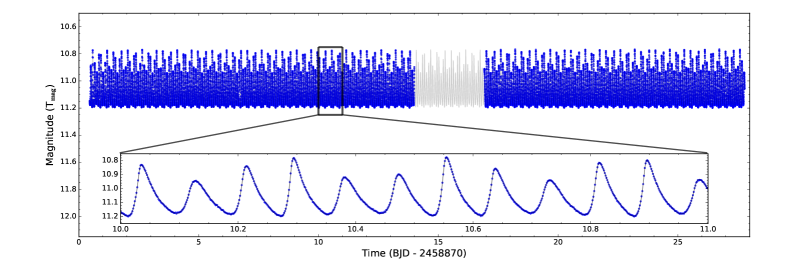
Figure 1: Light curves of AE UMa observed by TESS (blue points) and fitted by 65 extracted frequencies (gray line). The small panel is a zoom.

In this work, the pre-whitening process was performed to the light curves observed by TESS based on the framework introduced in Zong et al. (2016); Niu & Xue (2021), in which the uncertainties of amplitudes ($\sigma_{a}$) were defined as the median value of the amplitudes within a Lomb-Scargle spectral window of 2 $\,\mathrm{c}\ \mathrm{d}^{-1}$ equally divided by the frequency peak, while the uncertainties of frequencies ($\sigma_{f}$) were estimated following the formalism proposed by Montgomery & Odonoghue (1999); Aerts (2021). The statistical significant criterion of the signal-to-noise in the frequency spectrum was set to be 4.0 (Breger et al., 1993), and finally, 65 frequencies were extracted, which were composed by two independent frequencies ($f_{0}=11.6257\pm 0.0002\ \,\mathrm{c}\ \mathrm{d}^{-1}$ and $f_{1}=15.0314\pm 0.0002\ \,\mathrm{c}\ \mathrm{d}^{-1}$) and their harmonics and combinations. Figure 2 shows the origin frequency spectrum and the residues after extracting the 65 significant frequency solutions. All the significant frequency solutions are listed in Appendix, Table 2.

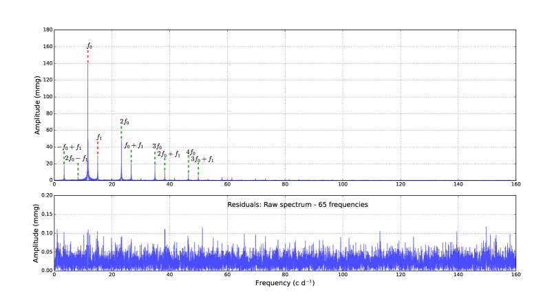
Figure 2: Frequency spectrum before (top panel) and after (bottom panel) the pre-whitening process. All the frequency peaks larger than 5 mmag are marked in the top panel.

The period ratio ($P_{1}/P_{0}=f_{0}/f_{1}$) has a value of 0.7734, which agrees with the theoretical calculated value ($\sim 0.77$, Petersen & Christensen-Dalsgaard (1996); Poretti et al. (2005)) and proves that these periods belong to the radial fundamental and first overtone pulsation modes.

2.2 Linear Period Variation Rate

The classical $O-C$ method was used to obtain the linear period variation rate of the fundamental pulsation mode. The TML were collected from the historical literatures, AAVSO, and TESS .

We collected 443 TML from Niu et al. (2017), and 23 more from the subsequent literatures. Based on the photometric data from AAVSO (from 1998 February to 2020 April) and TESS (from 2020 January 21 to 2020 February 18), we obtained the TML by a fourth polynomial fitting around the maxima in the light curves, whose uncertainties were estimated by Monte Carlo simulations. In this process, we determined 244 and 287 TML from AAVSO and TESS , respectively. All these TML except that from TESS were transformed into Barycentric Julian Dates based on the Barycentric Dynamical Time standard ($\rm{BJD_{TDB}}$) by using an online applets (Eastman et al., 2010). Finally, we had collected 997 TML lasting for about 46 years to perform the $O-C$ analysis, and all of them are listed in Appendix, Table 3. Those TML without giving uncertainties in the sources were uniformly estimated to give uncertainties based on their least significant digits from the sources.

A quadratic polynomials was used to reproduce the TML:

$$\,\mathrm{BJD}_{\,\mathrm{TDB}}=\,\mathrm{BJD}_{0}+P_{0}\cdot E+\frac{1}{2}\beta\cdot E^{2},$$ (1)

where $\,\mathrm{BJD}_{\,\mathrm{TDB}}$ is the TML, $\,\mathrm{BJD}_{0}$ is the reference epoch, $P_{0}$ is the period of the fundamental pulsation mode, $\beta$ is the linear change of pulsation period, and $E$ is the epoch.

The Markov Chain Monte Carlo (MCMC) algorithm was used to determine the posterior probability distribution of the parameters in Eq. (1). After the Markov Chains had been stable, the samples of the parameters were taken as their posterior probability distribution function (PDF) to obtain the mean values and the standard deviation of the parameters ($\,\mathrm{BJD}_{0}=2442062.58391(\pm 0.00001)$, $P_{0}=0.0860170616(\pm 0.0000000002)$, $\beta=6.0(\pm 0.1)\times 10^{-14}$). The best-fit result of the $O-C$ values and the corresponding residuals are shown in Figure 3. Based on the fitting results of $P_{0}$ and $\beta$, the linear period variation rate can be obtained as $\,(1/P_{0})(\,\mathrm{d}P_{0}/\,\mathrm{d}t)=(2.96\pm 0.05)\times 10^{-9}\ \,\mathrm{yr}^{-1}$. Here, one should note that the uncertainty of the value of $\,(1/P_{0})(\,\mathrm{d}P_{0}/\,\mathrm{d}t)$ decreases by a factor of about 40 compared with our previous work ($(5.4\pm 1.9)\times 10^{-9}\,\mathrm{yr}^{-1}$ in Niu et al. (2017)), which comes from both the additional TML and the different uncertainty estimation methods in these works.

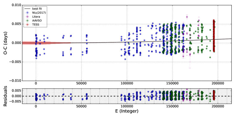
Figure 3: $O-C$ values and the corresponding residuals. In the upper panel, the black line represents the best-fit result of a quadratic fitting, the circles with different colors represent the different data sources. In the lower panel, the residuals of the best-fit result are plotted. The data collected from Niu et al. (2017) are shown in blue points; the data from historical literatures are shown in purple points; the data from AAVSO are shown in green points; the data from TESS are shown in red points. The $2\sigma$ (deep red) and $3\sigma$ (light red) bounds of the fitting results are also shown in the figures.

2.3 Theoretical Models

The stellar evolution code Modules for Experiments in Stellar Astrophysics (MESA; Paxton et al. (2011, 2013, 2015, 2018, 2019)) was used to build the structure and evolution models. The stellar oscillation code GYRE (Townsend & Teitler, 2013; Townsend et al., 2018; Goldstein & Townsend, 2020) was used to compute the corresponding frequencies of the pulsation modes for a specific structure model.

According to the previous work of Niu et al. (2017), we fix the initial helium mass fraction, metal mass fraction, and the mixing-length parameter as $Y=0.25$, $Z=0.008521$, and $\alpha_{MLT}=1.89$, respectively. In addition, the mass ranges from 1.50 $M_{\odot}$ to 2.50 $M_{\odot}$ with a step of 0.01 $M_{\odot}$. Considering AE UMa as an HADS with very slow rotation (Breger, 2000), the effect of rotation on the structure and evolution models were disregarded. Each of the evolutionary tracks were calculated from pre-MS to post-MS evolutionary stages. At every step in the evolutionary tracks, the frequencies of multiple pulsation modes were calculated.

The exponential overshooting scheme (Herwig, 2000) was tested with different $f_{\mathrm{ov}}$ values (obtained from Magic et al. (2010)). However, the best-fit with the the minimum value of $\chi^{2}$ (obtained by $f_{0}$ and $f_{1}$) results not only cannot give out effective temperature and luminosity values within uncertainties, but also showed large deviations to the observed linear period variation rate (exceeding 160%). As a result, the effect of overshooting were not included in our evolutionary models.

3 Results and Discussions

The best-fit model was determined by the observed fundamental and first overtone frequencies, which gave out the minimum value of $\chi^{2}$. Some of the important physical parameters of the best-fit model are listed in Table 1. The Hertzsprung-Russell diagram and $\log\,T_{\mathrm{eff}}$ vs $\log g$ diagram with all the evolutionary tracks and the best-fit model are shown in Figure 4, which represent that the effective temperature, the luminosity and the surface gravitational acceleration are all well matched between the observations and the theoretical predictions. The Petersen diagram and $\log P_{0}$ vs $\,(1/P_{0})(\,\mathrm{d}P_{0}/\,\mathrm{d}t)$ diagram are shown in Figure 5, which represent that not only the observed $P_{1}/P_{0}$ and $\log{P_{0}}$ match well with the calculated ones when the stellar mass equals to 1.59 $M_{\odot}$, but the linear period variation rate of the best-fit model also falls into the $20\%$ deviation region of the observed values.

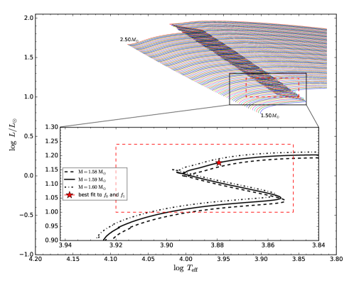
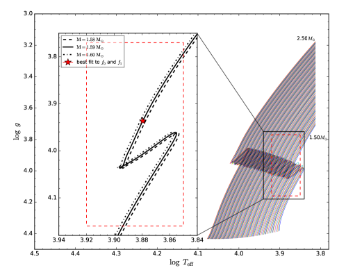
Figure 4: Hertzsprung-Russell diagram and $\log\,T_{\mathrm{eff}}$ vs $\log g$ diagram with all the evolutionary tracks and that of the best-fit model. The colored evolutionary tracks show from the zero-age MS to post-MS evolutionary stage, with initial mass from $1.50\ M_{\odot}$ to $2.50\ M_{\odot}$. The regions surrounded by the black rectangular boxes are selected to zoom in the observed constraints and the best-fit model, which are represented by the red dashed rectangular boxes and the red stars respectively.

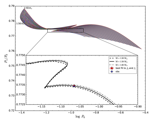
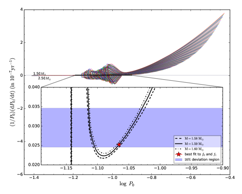
Figure 5: Petersen diagram and $\log P_{0}$ vs $\,(1/P_{0})(\,\mathrm{d}P_{0}/\,\mathrm{d}t)$ diagram with all the evolutionary tracks and that of the best-fit model. The colored evolutionary tracks show from the zero-age MS to post-MS evolutionary stage, with initial mass from $1.50\ M_{\odot}$ to $2.50\ M_{\odot}$. The regions surrounded by the black rectangular boxes are selected to zoom in the best-fit model, which are represented by the red stars. In the $\log P_{0}$ vs $\,(1/P_{0})(\,\mathrm{d}P_{0}/\,\mathrm{d}t)$ diagram, the blue region represents the 20% deviation region of the observed $\,(1/P_{0})(\,\mathrm{d}P_{0}/\,\mathrm{d}t)$.

Table 1: Some of the important parameters from observation and the best-fit model. The deviation in the last column is defined as $|(\,Q_{\mathrm{obs}}-\,Q_{\mathrm{mod}})/\,Q_{\mathrm{mod}}|$, where $\,Q_{\mathrm{obs}}$ is the observed quantity and $\,Q_{\mathrm{mod}}$ is the corresponding quantity from the theoretical model calculation.

Parameters	Observed	Best-fit	Deviation
$\,T_{\mathrm{eff}}\ \mathrm{(K)}$	$[7150,8320]$	$7575$	—
$\log L/L_{\odot}$	$[1.00,1.24]$	$1.18$	—
$\log g$	$[3.77,4.16]$	$3.94$	—
$f_{0}\ (\,\mathrm{c}\ \mathrm{d}^{-1})$	$11.6257\pm 0.0002$	$11.6259$	$0.0017\%$
$f_{1}\ (\,\mathrm{c}\ \mathrm{d}^{-1})$	$15.0314\pm 0.0002$	$15.0313$	$0.0007\%$
$\,(1/P_{0})(\,\mathrm{d}P_{0}/\,\mathrm{d}t)\ (\,\mathrm{yr}^{-1})$	$(2.96\pm 0.05)\times 10^{-9}$	$2.52\times 10^{-9}$	$17\%$
$\mathrm{Mass}\ (M_{\odot})$	—	$1.59$	—
$\mathrm{Age\ (Gyr)}$	—	$1.56$	—
$\log R/R_{\odot}$	—	$0.35$	—

These results prove that the observed linear period variation rate can be practically ascribed to the stellar evolution for AE UMa, which means that its evolutionary stage (post-MS) can be precisely determined in the framework of current stellar evolution theory. If we confirmed the evolutionary stages of more HADS and LADS in such way, we might have the answer to the question: why their light curves are so different from each other? On the other hand, the stellar evolution theory is precisely tested from the pre-MS to post-MS evolutionary stages within a deviation less than 20% by a single star rather than ensemble of stars. Although the 17% deviation could come from both the observation and theoretical model, it is a potential hint for updating the stellar evolution theory in future.

Although the concept of high-precision asteroseismology has been proposed and pioneeringly performed on some multi-modes pulsating stars (such as solar-like oscillation stars (Wu & Li, 2016, 2017), slowly pulsating B stars (Wu & Li, 2019), and red-giant branch stars (Zhang et al., 2020)) to precisely probe the stellar inner structure and test input physics, the involvement of period variation makes it possible for us to determine the evolutionary status of some pulsating stars (such as HADS (Niu et al., 2017; Xue et al., 2018) and blue large-amplitude pulsators (Wu & Li, 2018; Pigulski et al., 2022)). The observed period variation of the pulsating stars can be contributed by different mechanisms, such as stellar evolution (Niu et al., 2017; Xue et al., 2018), mass transfer (Xue & Niu, 2020), light traveling time effect in a multiple system (Xue & Niu, 2020), and nonlinear mode interactions (Breger & Montgomery, 2014; Zong et al., 2016; Bowman et al., 2016), which have different time scales. Generally speaking, the stellar evolution has the longest time scale (like the case of white dwarfs: Kepler et al. (2021)). If we selected some pulsating stars whose observed linear period variation rates falls into an interval derived from the theoretical predictions, we could have the opportunity to test and update the stellar evolution theory precisely by these single stars via the framework in this work. Here, we would like to propose the concept of Precise Evolutionary Asteroseismology (PEA). In PEA, we pay special attention to the above pulsating stars in different evolutionary stages. According to the comparison of the observed linear period variation rates and the theoretical predicted ones (according to asteroseismology), we can test the self-consistency of current stellar structure and evolution theory precisely in different evolutionary stages. The discrepancies can be used to guide further improvements or updates of the theory. At last, PEA will bring us a complete and precise stellar evolution theory to backtrack the history of each of these stars.

Appendix A Physical Parameters

The physical parameters (e.g., the effective temperature $\,T_{\mathrm{eff}}$, the effective surface gravity $\,\log{g}$ and the luminosity) show variations in a pulsation cycle of AE UMa. The effective temperature $\,T_{\mathrm{eff}}$ varies from 7150 K to 8320 K, and the effective surface gravity $\,\log{g}$ varies from 3.77 to 4.16 (Rodriguez et al., 1992; Hintz et al., 1997; Niu et al., 2017).

About the luminosity, we calculated it based on the distance, apparent magnitude, extinction, and bolometric correction. The absolute magnitude $M_{V}$ can be obtained following the formula

$$M_{V}=V-5\log{d}+5-A_{V}$$ (A1)

where $V=11.342$ mag was taken from AAVSO Photometric All Sky Survey (APASS) catalog (Henden et al., 2016), the distance $d=711$ pc was provided by Gaia DR3 (Bailer-Jones et al., 2021), the extinction $A_{V}=0.041$ mag was obtained from the maps of Schlafly & Finkbeiner (2011), and the lightness variation in $V$ band was about 0.6 mag (Niu et al., 2017).

On the other hand, the absolute bolometric magnitude $M_{bol}$ can be calculated from

$$M_{bol}=M_{V}+BC,$$ (A2)

where the empirical bolometric correction

$$BC=0.128\log{P}+0.022$$ (A3)

for $\delta$ Scuti stars, which was derived by Petersen & Christensen-Dalsgaard (1999).

Then, the luminosity can be obtained via

$$\log{L/L_{\odot}}=-0.4(M_{\rm{bol}}-M_{\rm{bol,\odot}})$$ (A4)

where the bolometric magnitude of the Sun $M_{\rm{bol,\odot}}=4.73$ mag was taken from Ref. (Torres, 2010). Finally, we got the range of the observed luminosity as $\log{L/L_{\odot}}\in[1.00,1.24]$.

Appendix B Long Tables

Table 2: Multi-frequency solution of the TESS Sector 21 light curves of AE UMa. Note: $\sigma_{f}$ denotes the error estimation of frequency, $\sigma_{a}$ denotes the error estimation of amplitude. S/N is calculated within a spectral window of 2 $\,\mathrm{c}\ \mathrm{d}^{-1}$ equally divided by the frequency peak.

NO.	Marks	Frequency $(\rm{c\ days^{-1}})$	$\sigma_{f}$ $(\rm{c\ days^{-1}})$	Amplitude (mmag)	$\sigma_{a}$ (mmag)	S/N
F1	$f_{0}$	11.6257	0.0002	139.81	1.69	82.57
F2	$2f_{0}$	23.2514	0.0003	48.90	0.63	77.80
F3	$f_{1}$	15.0314	0.0002	30.63	0.38	81.60
F4	$f_{0}+f_{1}$	26.6571	0.0003	20.63	0.26	79.42
F5	$-f_{0}+f_{1}$	3.4057	0.0003	18.70	0.23	80.47
F6	$3f_{0}$	34.8768	0.0003	18.38	0.23	78.37
F7	$2f_{0}+f_{1}$	38.2825	0.0003	11.21	0.14	79.01
F8	$4f_{0}$	46.5024	0.0003	8.39	0.12	70.07
F9	$3f_{0}+f_{1}$	49.9079	0.0003	6.15	0.08	73.10
F10	$2f_{0}-f_{1}$	8.2204	0.0003	5.13	0.07	68.95
F11	$5f_{0}$	58.1277	0.0004	3.81	0.07	57.40
F12	$4f_{0}+f_{1}$	61.5335	0.0003	3.28	0.06	57.67
F13	$f_{0}+2f_{1}$	41.6886	0.0004	2.99	0.06	50.31
F14	$2f_{1}$	30.0629	0.0004	2.98	0.06	46.91
F15	$5f_{0}+f_{1}$	73.1590	0.0004	2.23	0.04	52.41
F16	$3f_{0}-f_{1}$	19.8457	0.0005	2.17	0.05	39.56
F17	$6f_{0}$	69.7532	0.0005	2.06	0.04	46.76
F18	$2f_{0}+2f_{1}$	53.3136	0.0005	1.63	0.04	36.90
F19	$6f_{0}+f_{1}$	84.7849	0.0005	1.52	0.04	38.33
F20	$-f_{0}+2f_{1}$	18.4368	0.0005	1.45	0.04	38.83
F21	$7f_{0}$	81.3788	0.0006	1.21	0.04	32.91
F22	$3f_{0}+2f_{1}$	64.9389	0.0006	1.12	0.04	31.57
F23	$7f_{0}+f_{1}$	96.4101	0.0006	1.01	0.03	31.60
F24	$4f_{0}-f_{1}$	31.4717	0.0006	1.01	0.03	31.53
F25	$4f_{0}+2f_{1}$	76.5643	0.0008	0.87	0.03	26.28
F26	$-2f_{0}+2f_{1}$	6.8110	0.0009	0.78	0.04	21.30
F27	$5f_{0}+2f_{1}$	88.1900	0.0010	0.76	0.04	20.98
F28	$3f_{0}-2f_{1}$	4.8153	0.0008	0.74	0.03	25.00
F29	$8f_{0}$	93.0044	0.0009	0.72	0.03	23.00
F30	$8f_{0}+f_{1}$	108.0342	0.0009	0.65	0.03	21.70
F31	$5f_{0}-f_{1}$	43.0957	0.0009	0.63	0.03	21.62
F32	$6f_{0}-f_{1}$	54.7205	0.0011	0.61	0.03	18.52
F33	$6f_{0}+2f_{1}$	99.8155	0.0010	0.58	0.03	20.54
F34	$7f_{0}+2f_{1}$	111.4425	0.0011	0.52	0.03	18.94
F35	$7f_{0}-f_{1}$	66.3453	0.0010	0.52	0.03	20.33
F36	$f_{0}+3f_{1}$	56.7191	0.0014	0.44	0.03	14.72
F37	$4f_{0}-2f_{1}$	16.4431	0.0013	0.44	0.03	15.81
F38	$9f_{0}+f_{1}$	119.6604	0.0015	0.43	0.03	13.75
F39	$3f_{1}$	45.0948	0.0013	0.41	0.03	15.31
F40	$8f_{0}-f_{1}$	77.9740	0.0016	0.38	0.03	12.39
F41	$9f_{0}$	104.6287	0.0017	0.37	0.03	11.77
F42	$8f_{0}+2f_{1}$	123.0679	0.0016	0.34	0.03	12.73
F43	$5f_{0}-2f_{1}$	28.0635	0.0017	0.32	0.03	12.11
F44	$10f_{0}+f_{1}$	131.2863	0.0018	0.30	0.03	11.02
F45	$9f_{0}+2f_{1}$	134.6940	0.0020	0.29	0.03	10.02
F46	$9f_{0}-f_{1}$	89.5975	0.0023	0.24	0.03	8.84
F47	$10f_{0}$	116.2546	0.0027	0.24	0.03	7.58
F48	$2f_{0}+3f_{1}$	68.3446	0.0020	0.24	0.02	9.98
F49	$3f_{0}+3f_{1}$	79.9684	0.0025	0.22	0.03	8.10
F50	$4f_{0}+3f_{1}$	91.5941	0.0027	0.21	0.03	7.57
F51	$5f_{0}+3f_{1}$	103.2217	0.0027	0.21	0.03	7.37
F52	$10f_{0}+2f_{1}$	146.3188	0.0027	0.19	0.03	7.42
F53	$11f_{0}+f_{1}$	142.9116	0.0030	0.19	0.03	6.86
F54	$7f_{0}+3f_{1}$	126.4749	0.0027	0.18	0.02	7.47
F55	$6f_{0}-2f_{1}$	39.6944	0.0031	0.18	0.03	6.42
F56	$6f_{0}+3f_{1}$	114.8437	0.0033	0.18	0.03	6.11
F57	$8f_{0}+3f_{1}$	138.1003	0.0034	0.17	0.03	5.91
F58	$-f_{0}+3f_{1}$	33.4703	0.0037	0.16	0.03	5.49
F59	$10f_{0}-f_{1}$	101.2166	0.0039	0.14	0.03	5.12
F60	$-2f_{0}+3f_{1}$	21.8381	0.0043	0.13	0.03	4.74
F61	$12f_{0}+f_{1}$	154.5414	0.0043	0.13	0.03	4.71
F62	$5f_{0}-3f_{1}$	13.0325	0.0042	0.12	0.03	4.77
F63	$11f_{0}$	127.8854	0.0042	0.12	0.02	4.78
F64	$9f_{0}+3f_{1}$	149.7320	0.0050	0.12	0.03	4.06
F65	$7f_{0}-2f_{1}$	51.3246	0.0047	0.11	0.03	4.28

Table 3: All times of maximum light used in this work. $\sigma$: the uncertainties; Mark: the sources.

$\rm{BJD_{TDB}}$	$\sigma$	Mark	$\rm{BJD_{TDB}}$	$\sigma$	Mark	$\rm{BJD_{TDB}}$	$\sigma$	Mark
2442062.5837	0.0001	1	2454791.9945	0.0005	14	2457466.4354	0.0006	25
2442065.5964	0.0001	2	2454807.8229	0.0006	14	2457712.78688	0.00002	26
2442065.6783	0.0001	2	2454807.9039	0.0005	14	2457712.87055	0.00003	26
2442068.3437	0.0001	2	2454807.9873	0.0007	14	2457712.96264	0.00006	26
2442068.4307	0.0001	2	2454816.6800	0.0006	14	2457736.69950	0.00008	26
2442068.5208	0.0001	2	2454816.7619	0.0006	14	2457736.79017	0.00003	26
2442068.6034	0.0001	2	2454816.8508	0.0012	14	2457737.73234	0.00002	26
2442068.6876	0.0001	2	2454816.9406	0.0009	14	2457737.81526	0.00002	26
2442069.3813	0.0001	2	2454821.83920	0.00012	26	2457750.71793	0.00002	26
2442069.4656	0.0001	2	2454821.92866	0.00010	26	2457754.68162	0.00004	26
2442069.5478	0.0001	2	2454823.81476	0.00007	26	2457754.76328	0.00001	26
2442069.6368	0.0001	2	2454823.90464	0.00011	26	2457754.84626	0.00002	26
2442086.4970	0.0001	2	2454828.89354	0.00012	26	2457754.93784	0.00003	26
2442086.5792	0.0001	2	2454831.81665	0.00004	26	2457759.75330	0.00001	26
2442087.4395	0.0001	2	2454831.90727	0.00006	26	2457759.92720	0.00005	26
2442087.5268	0.0001	2	2454836.80564	0.00005	26	2457760.01375	0.00002	26
2442087.6160	0.0001	2	2454836.89619	0.00006	26	2457760.61471	0.00002	26
2442095.5303	0.0001	1	2454837.6644	0.0009	14	2457760.69625	0.00002	26
2442095.6128	0.0001	1	2454837.7572	0.0009	14	2457760.78462	0.00003	26
2442103.3518	0.0001	2	2454837.83872	0.00004	26	2457760.87458	0.00002	26
2442106.4528	0.0001	1	2454840.68081	0.00009	26	2457760.95547	0.00001	26
2442119.5257	0.0001	1	2454840.76418	0.00003	26	2457761.73499	0.00005	26
2442121.5030	0.0001	1	2454840.84693	0.00003	26	2457761.81728	0.00002	26
2442122.3633	0.0001	2	2454840.93604	0.00009	26	2457761.90007	0.00002	26
2442122.4489	0.0001	2	2454843.6893	0.0007	14	2457761.99147	0.00005	26
2442128.2973	0.0001	1	2454843.7711	0.0008	14	2457799.58143	0.00011	26
2442128.3877	0.0001	1	2454843.8574	0.0009	14	2457799.66695	0.00006	26
2442128.4732	0.0001	1	2454843.9501	0.0010	14	2457852.64846	0.00002	26
2442128.5562	0.0001	1	2454846.6144	0.0008	14	2457852.74036	0.00003	26
2442133.4632	0.0001	1	2454846.6967	0.0007	14	2458181.40908	0.00001	26
2442133.5447	0.0001	1	2454847.7343	0.0008	14	2458199.38347	0.00003	26
2442134.4060	0.0001	1	2454847.8171	0.0007	14	2458229.40617	0.00007	26
2442147.3938	0.0001	1	2454847.8995	0.0006	14	2458231.38243	0.00004	26
2442148.4300	0.0001	1	2454848.84885	0.00007	26	2458531.49304	0.00006	26
2442148.5122	0.0001	1	2454848.93873	0.00005	26	2458531.58339	0.00012	26
2442159.4370	0.0001	1	2454852.63050	0.00005	26	2458539.58589	0.00007	26
2442161.4150	0.0001	1	2454852.72310	0.00009	26	2458539.66642	0.00004	26
2442453.5311	0.0001	1	2454852.80649	0.00006	26	2458857.93322	0.00002	26
2442453.6142	0.0001	1	2454852.88857	0.00003	26	2458870.49564	0.00005	26
2442460.4994	0.0001	1	2454854.78810	0.00006	26	2458870.57721	0.00002	26
2442830.6285	0.0001	1	2454854.87030	0.00003	26	2458870.66063	0.00003	26
2442837.5125	0.0001	1	2454854.95318	0.00003	26	2458870.75379	0.00003	26
2442838.4596	0.0001	1	2454855.6476	0.0010	14	2458870.83771	0.00002	26
2442869.3382	0.0001	1	2454855.7323	0.0010	14	2458870.91910	0.00002	26
2442869.4210	0.0001	1	2454855.8126	0.0006	14	2458871.00836	0.00003	26
2443162.5713	0.0001	1	2454855.9030	0.0010	14	2458871.09802	0.00002	26
2444633.4631	0.0001	1	2454862.70116	0.00007	26	2458871.17798	0.00002	26
2444633.5445	0.0001	1	2454862.78468	0.00002	26	2458871.26286	0.00006	26
2444633.6314	0.0001	1	2454862.86687	0.00002	26	2458871.35589	0.00005	26
2444634.4051	0.0001	1	2454862.95571	0.00008	26	2458871.43830	0.00002	26
2444634.4907	0.0001	1	2454864.5880	0.0005	14	2458871.52069	0.00001	26
2444634.5815	0.0001	1	2454864.6731	0.0007	14	2458871.61190	0.00003	26
2444692.4714	0.0001	1	2454864.7656	0.0009	14	2458871.69903	0.00003	26
2445355.4908	0.0001	1	2454864.8484	0.0006	14	2458871.77983	0.00001	26
2445355.5733	0.0001	1	2454864.9303	0.0006	14	2458871.86637	0.00003	26
2445382.3234	0.0001	1	2454867.77368	0.00003	26	2458871.95815	0.00004	26
2445382.4110	0.0001	1	2454867.85560	0.00002	26	2458872.03962	0.00001	26
2445382.5003	0.0001	1	2454867.94563	0.00006	26	2458872.12341	0.00002	26
2445382.5813	0.0001	1	2454868.6353	0.0008	14	2458872.21532	0.00004	26
2446468.4607	0.0001	1	2454868.7173	0.0008	14	2458872.30044	0.00001	26
2446468.5474	0.0001	1	2454868.80341	0.00004	26	2458872.38140	0.00002	26
2446855.6285	0.0001	3	2454868.8040	0.0014	14	2458872.47010	0.00002	26
2446856.5735	0.0001	3	2454868.8948	0.0009	14	2458872.56038	0.00001	26
2446856.6567	0.0001	3	2454868.89492	0.00006	26	2458872.64117	0.00001	26
2446857.6023	0.0001	3	2454869.83759	0.00003	26	2458872.72584	0.00002	26
2446857.6931	0.0001	3	2454869.92022	0.00004	26	2458872.81831	0.00003	26
2446858.6388	0.0001	3	2454871.81962	0.00006	26	2458872.90151	0.00001	26
2446859.6672	0.0001	3	2454871.90141	0.00004	26	2458872.98277	0.00002	26
2446878.4187	0.0001	3	2454877.41053	0.00008	26	2458873.07347	0.00004	26
2446878.5070	0.0001	3	2454877.57609	0.00006	26	2458873.16169	0.00002	26
2446878.5952	0.0001	3	2454878.6942	0.0006	14	2458873.24229	0.00001	26
2446884.5268	0.0001	3	2454878.7818	0.0008	14	2458873.32889	0.00002	26
2446884.6123	0.0001	3	2454878.8728	0.0009	14	2458873.42074	0.00003	26
2446886.5913	0.0001	3	2454880.84619	0.00005	26	2458873.50236	0.00002	26
2450151.4571	0.0001	1	2454881.36027	0.00004	26	2458873.58521	0.00001	26
2450151.5391	0.0001	1	2454884.54483	0.00004	26	2458873.67699	0.00004	26
2450152.3177	0.0001	1	2454889.71021	0.00008	26	2458873.76298	0.00001	26
2450152.4869	0.0001	1	2454889.79400	0.00003	26	2458873.84329	0.00002	26
2450152.5763	0.0001	1	2454889.87645	0.00003	26	2458873.93138	0.00003	26
2450458.8822	0.0001	4	2454893.66178	0.00003	26	2458874.02252	0.00003	26
2450458.9643	0.0001	4	2454894.4419	0.0005	17	2458874.10328	0.00002	26
2450459.8247	0.0001	4	2454894.5234	0.0005	17	2458874.18748	0.00001	26
2450459.9120	0.0001	4	2454894.6078	0.0006	17	2458874.28015	0.00003	26
2450467.7395	0.0001	4	2454895.64489	0.00004	26	2458874.36398	0.00001	26
2450467.8243	0.0001	4	2454895.72587	0.00003	26	2458874.44476	0.00003	26
2450490.3614	0.0001	1	2454895.81257	0.00007	26	2458874.53515	0.00003	26
2450505.6704	0.0001	4	2454895.90468	0.00019	26	2458874.62426	0.00003	26
2450505.7602	0.0001	4	2454897.01955	0.00009	19	2458874.70470	0.00001	26
2450505.8468	0.0001	4	2454897.10767	0.00008	19	2458874.79012	0.00003	26
2450516.7683	0.0001	4	2454897.18907	0.00004	19	2458874.88281	0.00004	26
2450554.4439	0.0001	1	2454897.36693	0.00007	26	2458874.96478	0.00002	26
2450813.3557	0.0001	1	2454898.04976	0.0010	19	2458875.04727	0.00001	26
2450813.4415	0.0001	1	2454898.13391	0.0015	19	2458875.13891	0.00004	26
2450813.6158	0.0001	1	2454898.3091	0.0004	17	2458875.22538	0.00002	26
2450813.6992	0.0001	1	2454898.99384	0.00013	19	2458875.30597	0.00001	26
2450848.4547	0.0001	1	2454899.08448	0.00023	19	2458875.39338	0.00003	26
2450848.5398	0.0001	1	2454899.17137	0.00013	19	2458875.48491	0.00003	26
2450848.6219	0.0001	1	2454899.59626	0.00006	26	2458875.56600	0.00002	26
2450849.4822	0.0001	1	2454899.68821	0.00008	26	2458875.64951	0.00001	26
2450849.5695	0.0001	1	2454899.77260	0.00004	26	2458875.74197	0.00005	26
2450862.3847	0.0001	5	2454899.85460	0.00004	26	2458875.82662	0.00001	26
2450862.38719	0.00011	26	2454900.03261	0.00010	19	2458875.90783	0.00002	26
2450872.2816	0.0001	1	2454900.11364	0.0008	19	2458875.99683	0.00005	26
2450872.3641	0.0001	1	2454900.19858	0.00014	19	2458876.08681	0.00003	26
2450872.4488	0.0001	1	2454901.05834	0.00027	19	2458876.16728	0.00001	26
2450872.5401	0.0001	1	2454902.77954	0.00003	26	2458876.25200	0.00003	26
2450899.3736	0.0001	1	2454904.4206	0.0007	17	2458876.34479	0.00004	26
2450899.4577	0.0001	1	2454904.5013	0.0004	17	2458876.42775	0.00002	26
2450902.2983	0.0001	1	2454907.34502	0.00008	26	2458876.50956	0.00002	26
2450902.3826	0.0001	1	2454907.42676	0.00005	26	2458876.60048	0.00005	26
2450903.3328	0.0001	1	2454909.3154	0.0004	17	2458876.68821	0.00003	26
2450903.4199	0.0001	1	2454909.4094	0.0006	17	2458876.76860	0.00002	26
2450903.5016	0.0001	1	2454909.4902	0.0006	17	2458876.85513	0.00002	26
2451269.509	0.002	6	2454910.4342	0.0008	17	2458876.94718	0.00003	26
2451283.442	0.002	6	2454912.3330	0.0012	17	2458877.02860	0.00002	26
2451283.526	0.002	6	2454912.4153	0.0004	17	2458877.11156	0.00002	26
2451283.610	0.001	6	2454924.3749	0.0040	17	2458877.20379	0.00005	26
2451318.364	0.001	6	2454926.60542	0.00006	26	2458877.28943	0.000009	26
2451318.447	0.002	6	2454926.69757	0.00013	26	2458877.36994	0.00002	26
2451608.07238	0.00001	7	2454944.58674	0.00007	26	2458877.45800	0.00003	26
2451608.15849	0.00001	7	2454944.67459	0.00005	26	2458877.54912	0.00004	26
2451608.24027	0.00001	7	2454946.65202	0.00007	26	2458877.62968	0.00002	26
2451608.32715	0.00001	7	2454947.59993	0.00005	26	2458877.71348	0.00004	26
2451609.01933	0.00001	7	2454947.68109	0.00003	26	2458877.80691	0.00005	26
2451609.10137	0.00001	7	2454947.76600	0.00009	26	2458877.89003	0.00004	26
2451609.18725	0.00001	7	2454949.57565	0.00007	26	2458877.97193	0.00002	26
2451609.27776	0.00001	7	2454949.66396	0.00003	26	2458878.06198	0.00006	26
2451609.35903	0.00001	7	2454951.64071	0.00006	26	2458878.15057	0.00002	26
2451610.04573	0.00001	7	2454951.72793	0.00004	26	2458878.23097	0.00002	26
2451610.99764	0.00001	7	2454970.04393	0.00008	19	2458878.31738	0.00003	26
2451611.08286	0.00001	7	2454972.10855	0.00024	19	2458878.40948	0.00003	26
2451611.16345	0.00001	7	2455199.71023	0.00009	26	2458878.49120	0.00001	26
2451612.02532	0.00001	7	2455199.80216	0.00014	26	2458878.57373	0.00002	26
2451612.10980	0.00001	7	2455199.88467	0.00006	26	2458878.66541	0.00006	26
2451612.20179	0.00001	7	2455202.63391	0.00008	26	2458878.75171	0.00002	26
2451612.28538	0.00001	7	2455202.72659	0.00015	26	2458878.83250	0.00001	26
2451612.37118	0.00001	7	2455202.80999	0.00007	26	2458878.92007	0.00005	26
2451612.96996	0.00001	7	2455223.44980	0.00004	26	2458879.01134	0.00003	26
2451613.06164	0.00001	7	2455223.54053	0.00006	26	2458879.09225	0.00003	26
2451613.14610	0.00001	7	2455223.62840	0.00005	26	2458879.17607	0.00003	26
2451613.22839	0.00001	7	2455230.24632	0.00009	19	2458879.26871	0.00006	26
2451613.31631	0.00001	7	2455230.33867	0.00010	19	2458879.35296	0.00003	26
2451615.03489	0.00001	7	2455230.42086	0.00008	19	2458879.43417	0.00002	26
2451615.12679	0.00001	7	2455231.28257	0.00008	19	2458879.52368	0.00004	26
2451615.21055	0.00001	7	2455231.36431	0.00006	19	2458879.61314	0.00002	26
2451615.29269	0.00001	7	2455233.34646	0.00003	26	2458879.69355	0.00002	26
2451615.98622	0.00001	7	2455233.42847	0.00002	26	2458879.77905	0.00002	26
2451616.07122	0.00001	7	2455233.51836	0.00004	26	2458879.87182	0.00004	26
2451616.15338	0.00001	7	2455233.60682	0.00003	26	2458879.95373	0.00003	26
2451616.23960	0.00001	7	2455238.76197	0.00005	26	2458880.03596	0.00002	26
2451929.25633	0.00001	7	2455244.44561	0.00004	26	2458880.12706	0.00008	26
2451929.34714	0.00001	7	2455244.52721	0.00002	26	2458880.21440	0.00003	26
2451930.20658	0.00001	7	2455244.61083	0.00003	26	2458880.29527	0.00002	26
2451930.28924	0.00001	7	2455244.70247	0.00007	26	2458880.38204	0.00003	26
2451930.37279	0.00001	7	2455257.69079	0.00004	26	2458880.47386	0.00003	26
2451931.23228	0.00001	7	2455257.77210	0.00002	26	2458880.55507	0.00002	26
2451931.32102	0.00001	7	2455259.4115	0.0014	18	2458880.63841	0.00001	26
2451941.21094	0.00001	7	2455259.66868	0.00009	26	2458880.73072	0.00004	26
2451941.29867	0.00001	7	2455259.75465	0.00005	26	2458880.81559	0.00002	26
2451941.38884	0.00001	7	2455266.46539	0.00006	26	2458880.89664	0.00002	26
2451942.15698	0.00001	7	2455266.54739	0.00005	26	2458880.98571	0.00013	26
2451942.24803	0.00001	7	2455266.63087	0.00007	26	2458881.07546	0.00005	26
2451942.33180	0.00001	7	2455279.62366	0.00010	26	2458881.15606	0.00003	26
2451942.41487	0.00001	7	2455279.71180	0.00007	26	2458881.24108	0.00003	26
2452321.4096	0.0008	8	2455282.63677	0.00005	26	2458881.33315	0.00006	26
2452371.3843	0.0002	8	2455282.71747	0.00003	26	2458881.41665	0.00002	26
2452685.3467	0.0012	8	2455293.3833	0.0010	18	2458881.49844	0.00003	26
2452685.4376	0.0012	8	2455293.4759	0.0007	18	2458881.58896	0.00006	26
2452730.4194	0.0004	8	2455298.62926	0.00003	26	2458881.67686	0.00003	26
2452739.3624	0.0007	8	2455301.64383	0.00007	26	2458881.75726	0.00004	26
2452745.4709	0.0004	9	2455301.73217	0.00005	26	2458881.84352	0.00003	26
2452980.5615	0.0011	10	2455302.3325	0.0009	18	2458881.93608	0.00003	26
2452980.6428	0.0011	10	2455303.3598	0.0014	18	2458882.01766	0.00002	26
2452980.7286	0.0011	10	2455304.3966	0.0007	18	2458882.10057	0.00003	26
2453003.5238	0.0004	9	2455304.4782	0.0010	18	2458882.19256	0.00005	26
2453028.2949	0.0006	9	2455305.3395	0.0007	18	2458882.27817	0.00002	26
2453028.3878	0.0010	9	2455305.4245	0.0014	18	2458882.35909	0.00002	26
2453028.4712	0.0005	9	2455309.3855	0.0008	18	2458882.44663	0.00006	26
2453028.5529	0.0006	9	2455310.4131	0.0019	18	2458882.53785	0.00004	26
2453028.6427	0.0011	9	2455311.3669	0.0007	18	2458882.61895	0.00001	26
2453069.4126	0.0016	9	2455311.4495	0.0005	18	2458882.70329	0.00003	26
2453069.5036	0.0018	9	2455314.63560	0.00008	26	2458882.79554	0.00007	26
2453070.4500	0.0013	9	2455554.87787	0.00003	26	2458882.87923	0.00003	26
2453070.533	0.002	9	2455554.96003	0.00003	26	2458882.96052	0.00004	26
2453090.4060	0.0027	9	2455555.73931	0.00003	26	2458883.05111	0.00008	26
2453094.3582	0.0010	9	2455555.82099	0.00002	26	2458883.13989	0.00002	26
2453110.3626	0.0019	12	2455555.90869	0.00007	26	2458883.21988	0.00002	26
2453409.52929	0.00024	11	2455562.79234	0.00004	26	2458883.30536	0.00006	26
2453409.61157	0.00032	11	2455562.87351	0.00004	26	2458883.39844	0.00009	26
2453409.69477	0.00058	11	2455562.96285	0.00011	26	2458883.48044	0.00002	26
2453427.3279	0.0011	12	2455583.43210	0.00012	19	2458883.56278	0.00005	26
2453427.4188	0.0012	12	2455584.37947	0.00018	19	2458883.65416	0.00003	26
2453427.5038	0.0012	12	2455584.55239	0.00008	26	2458883.74089	0.00002	26
2453451.4143	0.0022	10	2455584.63618	0.00008	26	2458883.82168	0.00001	26
2453451.5049	0.0024	10	2455584.72789	0.00014	26	2458883.90864	0.00003	26
2453484.3623	0.0024	10	2455584.81253	0.00006	26	2458886.74639	0.00002	26
2453765.3810	0.0002	13	2455584.89442	0.00006	26	2458886.83222	0.00004	26
2453765.4667	0.0002	13	2455584.98193	0.00019	26	2458886.92482	0.00007	26
2453765.5469	0.0002	13	2455585.41399	0.00008	19	2458886.92486	0.00007	26
2453766.3285	0.0002	13	2455587.39535	0.00009	19	2458887.00676	0.00003	26
2453766.4086	0.0002	13	2455588.42086	0.00008	19	2458887.08949	0.00003	26
2453766.4950	0.0002	13	2455607.95360	0.00018	19	2458887.18135	0.00003	26
2453766.5856	0.0002	13	2455608.03562	0.00011	19	2458887.26740	0.00003	26
2453794.3626	0.0003	11	2455608.11878	0.00011	19	2458887.34802	0.00002	26
2453795.3122	0.0003	11	2455608.21064	0.00022	19	2458887.43575	0.00004	26
2453795.4005	0.0001	11	2455608.29613	0.00012	19	2458887.52696	0.00004	26
2453827.6577	0.0013	11	2455608.37710	0.00011	19	2458887.60792	0.00002	26
2453827.65791	0.00014	26	2455610.35990	0.00010	19	2458887.69180	0.00003	26
2454037.88265	0.00013	26	2455611.38852	0.00016	19	2458887.78471	0.00005	26
2454050.87089	0.00013	26	2455612.24770	0.00014	19	2458887.86849	0.00002	26
2454050.95159	0.00010	26	2455612.33995	0.00022	19	2458887.94978	0.00002	26
2454056.80189	0.00008	26	2455613.19877	0.00021	19	2458888.03946	0.00009	26
2454056.88685	0.00007	26	2455616.98081	0.00011	19	2458888.12864	0.00003	26
2454079.7673	0.0007	14	2455617.07131	0.00008	19	2458888.20918	0.00002	26
2454079.8587	0.0014	14	2455617.15276	0.00005	19	2458888.29435	0.00004	26
2454079.9444	0.0007	14	2455617.23661	0.00006	19	2458888.38707	0.00005	26
2454087.77092	0.00012	26	2455617.32888	0.00010	19	2458888.46953	0.00002	26
2454102.6478	0.0006	14	2455620.07795	0.00010	19	2458888.55188	0.00001	26
2454102.7372	0.0015	14	2455620.16102	0.00017	19	2458888.64285	0.00005	26
2454102.8261	0.0009	14	2455620.33798	0.00007	26	2458888.72998	0.00002	26
2454103.6856	0.0009	14	2455621.11110	0.00017	19	2458888.81072	0.00002	26
2454103.7684	0.0012	14	2455621.19938	0.00019	19	2458888.89759	0.00003	26
2454104.7124	0.0009	14	2455878.81472	0.00003	26	2458888.98939	0.00002	26
2454107.6365	0.0005	14	2455878.90285	0.00005	26	2458889.07032	0.00003	26
2454107.7258	0.0009	14	2455890.77593	0.00008	26	2458889.15393	0.00002	26
2454107.8145	0.0010	14	2455890.85714	0.00007	26	2458889.24631	0.00004	26
2454107.8951	0.0007	14	2455890.94564	0.00012	26	2458889.33116	0.00002	26
2454110.7395	0.0011	14	2455907.72203	0.00012	26	2458889.41215	0.00001	26
2454110.8214	0.0006	14	2455907.80705	0.00007	26	2458889.50077	0.00006	26
2454110.90530	0.00009	26	2455931.71546	0.00010	26	2458889.59125	0.00003	26
2454110.9058	0.0007	14	2455931.80728	0.00016	26	2458889.67192	0.00002	26
2454110.9984	0.0007	14	2455937.39891	0.00012	19	2458889.75649	0.00002	26
2454115.72933	0.00013	26	2455961.30584	0.00004	19	2458889.84925	0.00004	26
2454121.66129	0.00009	26	2455961.39147	0.00010	19	2458889.93229	0.00002	26
2454121.74340	0.00009	26	2455964.31556	0.00014	19	2458890.01399	0.00002	26
2454125.7063	0.0010	14	2455964.40805	0.00019	19	2458890.10432	0.00007	26
2454125.7890	0.0011	14	2455966.21408	0.00007	19	2458890.19276	0.00002	26
2454125.8723	0.0008	14	2455966.29493	0.00005	19	2458890.27331	0.00002	26
2454125.9656	0.0014	14	2455966.38042	0.00008	19	2458890.35946	0.00005	26
2454131.5557	0.0013	14	2455967.33183	0.00009	19	2458890.45191	0.00006	26
2454131.6399	0.0008	14	2455967.41669	0.00007	19	2458890.53334	0.00002	26
2454131.7219	0.0006	14	2455968.27811	0.00007	19	2458890.61635	0.00002	26
2454131.8113	0.0011	14	2455968.35894	0.00004	19	2458890.70829	0.00005	26
2454131.8996	0.0006	14	2455969.30458	0.00007	19	2458890.79389	0.00001	26
2454136.5453	0.0011	14	2455969.39671	0.00014	19	2458890.87450	0.00003	26
2454136.6282	0.0006	14	2455984.4479	0.0014	20	2458890.96239	0.00005	26
2454136.7111	0.0008	14	2455993.30430	0.0005	22	2458891.05366	0.00003	26
2454136.8005	0.0009	14	2455993.38780	0.0005	22	2458891.13421	0.00002	26
2454136.8889	0.0007	14	2455997.00877	0.00008	19	2458891.21844	0.00003	26
2454136.9704	0.0012	14	2455997.09141	0.00004	19	2458891.31115	0.00005	26
2454137.6588	0.0013	14	2455997.17372	0.00004	19	2458891.39493	0.00001	26
2454137.7498	0.0014	14	2455997.26468	0.00010	19	2458891.56607	0.00009	26
2454137.8318	0.0009	14	2455998.03450	0.00008	19	2458891.65506	0.00004	26
2454139.7233	0.0009	14	2455998.12286	0.00014	19	2458891.73556	0.00002	26
2454139.8131	0.0008	14	2455998.21269	0.00008	19	2458891.82131	0.00003	26
2454139.8949	0.0005	14	2455998.29351	0.00006	19	2458891.91382	0.00005	26
2454141.7883	0.0010	14	2455998.98155	0.00009	19	2458891.99596	0.00002	26
2454141.8775	0.0007	14	2455999.07344	0.00009	19	2458892.07860	0.00001	26
2454141.9582	0.0009	14	2455999.15543	0.00005	19	2458892.17001	0.00005	26
2454151.67767	0.00009	26	2455999.23823	0.00005	19	2458892.25648	0.00003	26
2454151.76589	0.00027	26	2456000.01689	0.00005	19	2458892.33707	0.00002	26
2454152.6248	0.0011	14	2456000.09857	0.00004	19	2458892.42443	0.00003	26
2454153.5753	0.0010	14	2456000.18819	0.00009	19	2458892.51619	0.00004	26
2454154.6890	0.0010	14	2456000.27695	0.00006	19	2458892.59699	0.00002	26
2454154.7807	0.0009	14	2456001.04671	0.00006	19	2458892.68062	0.00002	26
2454154.8625	0.0006	14	2456001.13759	0.00006	19	2458892.77309	0.00006	26
2454164.66673	0.00021	26	2456001.21934	0.00003	19	2458892.85766	0.00001	26
2454164.75938	0.00022	26	2456001.30305	0.00006	19	2458892.93896	0.00001	26
2454171.4671	0.0023	15	2456002.4214	0.0006	23	2458893.02790	0.00007	26
2454175.4213	0.0013	15	2456006.4683	0.0001	23	2458893.11768	0.00004	26
2454184.62265	0.00008	26	2456008.3559	0.0008	23	2458893.19803	0.00004	26
2454184.71548	0.00019	26	2456008.4486	0.0012	23	2458893.28354	0.00002	26
2454188.58406	0.00010	26	2456009.4745	0.0007	23	2458893.37609	0.00005	26
2454188.66520	0.00008	26	2456014.4250	0.0014	23	2458893.45861	0.00002	26
2454188.75249	0.00011	26	2456062.03196	0.00005	19	2458893.54076	0.00002	26
2454196.4983	0.0009	15	2456063.06986	0.00015	19	2458893.63166	0.00005	26
2454197.360	0.002	15	2456064.01443	0.00008	19	2458893.71907	0.00002	26
2454197.4409	0.0006	15	2456064.09555	0.00008	19	2458893.79966	0.00003	26
2454198.3857	0.0009	15	2456065.04265	0.00009	19	2458893.88622	0.00002	26
2454198.4748	0.0007	15	2456068.05875	0.00021	19	2458893.97844	0.00003	26
2454202.4295	0.0007	15	2456319.65508	0.00008	26	2458894.05964	0.00002	26
2454220.58298	0.00009	26	2456319.74464	0.00005	26	2458894.14297	0.00002	26
2454220.66380	0.00007	26	2456325.41563	0.00019	26	2458894.23523	0.00005	26
2454414.8946	0.0008	14	2456326.45390	0.00033	26	2458894.32016	0.00003	26
2454414.9811	0.0007	14	2456342.3651	0.0003	21	2458894.40103	0.00003	26
2454417.7278	0.0006	14	2456342.4468	0.0003	21	2458894.48951	0.00005	26
2454417.9065	0.0006	14	2456342.5322	0.0009	21	2458894.58014	0.00003	26
2454417.9863	0.0005	14	2456342.6275	0.0005	21	2458894.66095	0.00001	26
2454422.89521	0.00011	26	2456610.73911	0.00006	26	2458894.74553	0.00002	26
2454440.6965	0.0010	14	2456610.82011	0.00005	26	2458894.83840	0.00005	26
2454442.7626	0.0009	14	2456610.90597	0.00009	26	2458894.92140	0.00002	26
2454442.8523	0.0011	14	2456615.72836	0.00009	26	2458895.00300	0.00002	26
2454442.9349	0.0013	14	2456615.80960	0.00007	26	2458895.09339	0.00006	26
2454451.6250	0.0012	14	2456619.77091	0.00006	26	2458895.18162	0.00002	26
2454460.6520	0.0008	14	2456620.71765	0.00003	26	2458895.26206	0.00002	26
2454460.7440	0.0007	14	2456620.79864	0.00001	26	2458895.34793	0.00003	26
2454460.8254	0.0005	14	2456620.88433	0.00017	26	2458895.44038	0.00004	26
2454460.9096	0.0006	14	2456623.4632	0.0035	24	2458895.52239	0.00002	26
2454467.7962	0.0006	14	2456633.70225	0.00003	26	2458895.60523	0.00002	26
2454468.7399	0.0006	14	2456633.78654	0.00002	26	2458895.69693	0.00006	26
2454468.8227	0.0007	14	2456642.4783	0.0009	24	2458895.78285	0.00002	26
2454468.9127	0.0009	14	2456642.5592	0.0006	24	2458895.86363	0.00002	26
2454469.6822	0.0006	14	2456642.6494	0.0011	24	2458895.95121	0.00003	26
2454469.7708	0.0008	14	2456643.5068	0.0035	24	2458896.04261	0.00004	26
2454469.8610	0.0006	14	2456655.72285	0.00004	26	2458896.12321	0.00002	26
2454469.9421	0.0006	14	2456660.63037	0.00004	26	2458896.20721	0.00003	26
2454474.76018	0.00015	26	2456660.71202	0.00002	26	2458896.30018	0.00004	26
2454474.85028	0.00011	26	2456660.79912	0.00007	26	2458896.38403	0.00001	26
2454474.93116	0.00009	26	2456660.88863	0.00007	26	2458896.46539	0.00003	26
2454479.83930	0.00016	26	2456660.97184	0.00002	26	2458896.55462	0.00006	26
2454479.92088	0.00010	26	2456722.47037	0.00017	26	2458896.64411	0.00004	26
2454506.41171	0.00010	26	2456730.47608	0.00026	26	2458896.72477	0.00003	26
2454506.50304	0.00012	26	2456732.36386	0.00006	26	2458896.81005	0.00004	26
2454506.5894	0.0006	16	2456744.40612	0.00008	26	2458896.90268	0.00006	26
2454512.5206	0.0002	16	2456998.93336	0.00014	26	2458896.98505	0.00002	26
2454513.38185	0.00001	26	2456999.01415	0.00026	26	2458897.06724	0.00001	26
2454513.46540	0.00001	26	2457158.40951	0.00003	26	2458897.15865	0.00004	26
2454513.4657	0.0009	16	2457390.73645	0.00003	26	2458897.24531	0.00003	26
2454513.5566	0.0009	16	2457392.63658	0.00005	26	2458897.32620	0.00002	26
2454513.55706	0.00003	26	2457392.71836	0.00001	26	2458897.41347	0.00005	26
2454516.82745	0.00010	26	2457392.80048	0.00002	26	2458897.50480	0.00004	26
2454524.4822	0.0008	16	2457392.89186	0.00003	26	2458897.50484	0.00002	26
2454769.8866	0.0010	14	2457392.97894	0.00002	26	2458897.58612	0.00002	26
2454770.8343	0.0005	14	2457406.65009	0.00005	26	2458897.58621	0.00003	26
2454770.9159	0.0005	14	2457406.74123	0.00004	26	2458897.66929	0.00005	26
2454781.8391	0.0007	14	2457406.82499	0.00002	26	2458897.66944	0.00002	26
2454781.9308	0.0010	14	2457406.90866	0.00003	26	2458897.76197	0.00002	26
2454788.8087	0.0006	14	2457425.4941	0.0010	25	2458897.76199	0.00004	26
2454788.8919	0.0006	14	2457425.5774	0.0010	25	2458912.63614	0.00002	26
2454788.9840	0.0012	14	2457425.6596	0.0010	25	2458951.34527	0.00005	26
2454791.7340	0.0006	14	2457437.44382	0.00001	26	2458962.36194	0.00015	26
2454791.8164	0.0005	14	2457466.3535	0.0009	25	2458962.44653	0.00006	26
2454791.9087	0.0011	14

Note. — Source: (1) Pócs & Szeidl (2001); (2) Broglia & Conconi (1975); (3) Rodriguez et al. (1992); (4) Hintz et al. (1997); (5) Agerer et al. (1999); (6) Pejcha et al. (2001); (7) Zhou (2001); (8) Agerer & Hubscher (2003); (9) Hubscher (2005); (10) Hubscher et al. (2005); (11) Klingenberg et al. (2006); (12) Hubscher et al. (2006); (13) Hubscher & Walter (2007); (14) Samolyk (2010); (15) Hubscher (2007); (16)Hubscher et al. (2009); (17) Hubscher et al. (2010); (18) Hubscher & Monninger (2011); (19) Niu et al. (2017); (20) Hubscher & Lehmann (2012); (21) Hubscher (2013); (22) Hubscher & Lehmann (2013); (23) Hubscher et al. (2013); (24) Hubscher (2014); (25) Hubscher (2017); (26) this work.

References

- Aerts (2021) Aerts, C. 2021, Rev. Mod. Phys., 93, 015001, doi: 10.1103/RevModPhys.93.015001
- Agerer et al. (1999) Agerer, F., Dahm, M., & Hubscher, J. 1999, Information Bulletin on Variable Stars, 4712, 1
- Agerer & Hubscher (2003) Agerer, F., & Hubscher, J. 2003, Information Bulletin on Variable Stars, 5485, 1
- Bailer-Jones et al. (2021) Bailer-Jones, C. A. L., Rybizki, J., Fouesneau, M., Demleitner, M., & Andrae, R. 2021, AJ, 161, 147, doi: 10.3847/1538-3881/abd806
- Bowman et al. (2021) Bowman, D. M., Hermans, J., Daszyńska-Daszkiewicz, J., et al. 2021, MNRAS, 504, 4039, doi: 10.1093/mnras/stab1124
- Bowman et al. (2016) Bowman, D. M., Kurtz, D. W., Breger, M., Murphy, S. J., & Holdsworth, D. L. 2016, MNRAS, 460, 1970, doi: 10.1093/mnras/stw1153
- Breger (2000) Breger, M. 2000, in Astronomical Society of the Pacific Conference Series, Vol. 210, Delta Scuti and Related Stars, ed. M. Breger & M. Montgomery, 3
- Breger & Montgomery (2014) Breger, M., & Montgomery, M. H. 2014, ApJ, 783, 89, doi: 10.1088/0004-637X/783/2/89
- Breger & Pamyatnykh (1998) Breger, M., & Pamyatnykh, A. A. 1998, A&A, 332, 958. https://arxiv.org/abs/astro-ph/9802076
- Breger et al. (1993) Breger, M., Stich, J., Garrido, R., et al. 1993, A&A, 271, 482
- Broglia & Conconi (1975) Broglia, P., & Conconi, P. 1975, A&AS, 22, 243
- Daszyńska-Daszkiewicz et al. (2022) Daszyńska-Daszkiewicz, J., Walczak, P., Pamyatnykh, A. A., & Szewczuk, W. 2022, MNRAS, 512, 3551, doi: 10.1093/mnras/stac646
- Eastman et al. (2010) Eastman, J., Siverd, R., & Gaudi, B. S. 2010, PASP, 122, 935, doi: 10.1086/655938
- Foreman-Mackey et al. (2013) Foreman-Mackey, D., Hogg, D. W., Lang, D., & Goodman, J. 2013, PASP, 125, 306, doi: 10.1086/670067
- Goldstein & Townsend (2020) Goldstein, J., & Townsend, R. H. D. 2020, ApJ, 899, 116, doi: 10.3847/1538-4357/aba748
- Handler (2009) Handler, G. 2009, in American Institute of Physics Conference Series, Vol. 1170, Stellar Pulsation: Challenges for Theory and Observation, ed. J. A. Guzik & P. A. Bradley, 403–409, doi: 10.1063/1.3246528
- Henden et al. (2016) Henden, A. A., Templeton, M., Terrell, D., et al. 2016, VizieR Online Data Catalog, II/336
- Herwig (2000) Herwig, F. 2000, A&A, 360, 952. https://arxiv.org/abs/astro-ph/0007139
- Hintz et al. (1997) Hintz, E., Hintz, M. L., & Joner, M. D. 1997, PASP, 109, 1073, doi: 10.1086/133977
- Holdsworth et al. (2014) Holdsworth, D. L., Smalley, B., Gillon, M., et al. 2014, MNRAS, 439, 2078, doi: 10.1093/mnras/stu094
- Hubscher (2005) Hubscher, J. 2005, Information Bulletin on Variable Stars, 5643, 1
- Hubscher (2007) —. 2007, Information Bulletin on Variable Stars, 5802, 1
- Hubscher (2013) —. 2013, Information Bulletin on Variable Stars, 6084, 1
- Hubscher (2014) —. 2014, Information Bulletin on Variable Stars, 6118, 1
- Hubscher (2017) —. 2017, Information Bulletin on Variable Stars, 6196, 1, doi: 10.22444/IBVS.6196
- Hubscher et al. (2013) Hubscher, J., Braune, W., & Lehmann, P. B. 2013, Information Bulletin on Variable Stars, 6048, 1
- Hubscher & Lehmann (2012) Hubscher, J., & Lehmann, P. B. 2012, Information Bulletin on Variable Stars, 6026, 1
- Hubscher & Lehmann (2013) —. 2013, Information Bulletin on Variable Stars, 6070, 1
- Hubscher et al. (2010) Hubscher, J., Lehmann, P. B., Monninger, G., Steinbach, H.-M., & Walter, F. 2010, Information Bulletin on Variable Stars, 5918, 1
- Hubscher & Monninger (2011) Hubscher, J., & Monninger, G. 2011, Information Bulletin on Variable Stars, 5959, 1
- Hubscher et al. (2005) Hubscher, J., Paschke, A., & Walter, F. 2005, Information Bulletin on Variable Stars, 5657, 1
- Hubscher et al. (2006) —. 2006, Information Bulletin on Variable Stars, 5731, 1
- Hubscher et al. (2009) Hubscher, J., Steinbach, H.-M., & Walter, F. 2009, Information Bulletin on Variable Stars, 5874, 1
- Hubscher & Walter (2007) Hubscher, J., & Walter, F. 2007, Information Bulletin on Variable Stars, 5761, 1
- Jenkins et al. (2016) Jenkins, J. M., Twicken, J. D., McCauliff, S., et al. 2016, in Society of Photo-Optical Instrumentation Engineers (SPIE) Conference Series, Vol. 9913, Software and Cyberinfrastructure for Astronomy IV, ed. G. Chiozzi & J. C. Guzman, 99133E, doi: 10.1117/12.2233418
- Kepler et al. (2021) Kepler, S. O., Winget, D. E., Vanderbosch, Z. P., et al. 2021, ApJ, 906, 7, doi: 10.3847/1538-4357/abc626
- Klingenberg et al. (2006) Klingenberg, G., Dvorak, S. W., & Robertson, C. W. 2006, Information Bulletin on Variable Stars, 5701, 1
- Magic et al. (2010) Magic, Z., Serenelli, A., Weiss, A., & Chaboyer, B. 2010, ApJ, 718, 1378, doi: 10.1088/0004-637X/718/2/1378
- Montgomery & Odonoghue (1999) Montgomery, M. H., & Odonoghue, D. 1999, Delta Scuti Star Newsletter, 13, 28
- Niu et al. (2013) Niu, J.-S., Fu, J.-N., & Zong, W.-K. 2013, Res. Astron. Astrophys. , 13, 1181, doi: 10.1088/1674-4527/13/10/004
- Niu & Li (2018) Niu, J.-S., & Li, T. 2018, Phys. Rev. D, 97, 023015, doi: 10.1103/PhysRevD.97.023015
- Niu et al. (2018) Niu, J.-S., Li, T., Ding, R., et al. 2018, Phys. Rev. D, 97, 083012, doi: 10.1103/PhysRevD.97.083012
- Niu et al. (2019) Niu, J.-S., Li, T., & Xue, H.-F. 2019, ApJ, 873, 77, doi: 10.3847/1538-4357/ab0420
- Niu & Xue (2021) Niu, J.-S., & Xue, H.-F. 2021, arXiv e-prints, arXiv:2102.10259. https://arxiv.org/abs/2102.10259
- Niu et al. (2017) Niu, J.-S., Fu, J.-N., Li, Y., et al. 2017, MNRAS, 467, 3122, doi: 10.1093/mnras/stx125
- Paxton et al. (2011) Paxton, B., Bildsten, L., Dotter, A., et al. 2011, ApJS, 192, 3, doi: 10.1088/0067-0049/192/1/3
- Paxton et al. (2013) Paxton, B., Cantiello, M., Arras, P., et al. 2013, ApJS, 208, 4, doi: 10.1088/0067-0049/208/1/4
- Paxton et al. (2015) Paxton, B., Marchant, P., Schwab, J., et al. 2015, ApJS, 220, 15, doi: 10.1088/0067-0049/220/1/15
- Paxton et al. (2018) Paxton, B., Schwab, J., Bauer, E. B., et al. 2018, ApJS, 234, 34, doi: 10.3847/1538-4365/aaa5a8
- Paxton et al. (2019) Paxton, B., Smolec, R., Schwab, J., et al. 2019, ApJS, 243, 10, doi: 10.3847/1538-4365/ab2241
- Pejcha et al. (2001) Pejcha, O., Havlik, T., & Kral, L. 2001, Information Bulletin on Variable Stars, 5080, 1
- Petersen & Christensen-Dalsgaard (1996) Petersen, J. O., & Christensen-Dalsgaard, J. 1996, A&A, 312, 463
- Petersen & Christensen-Dalsgaard (1999) —. 1999, A&A, 352, 547
- Pigulski et al. (2022) Pigulski, A., Kotysz, K., & Kołaczek-Szymański, P. A. 2022, A&A, 663, A62, doi: 10.1051/0004-6361/202243293
- Pócs & Szeidl (2001) Pócs, M. D., & Szeidl, B. 2001, A&A, 368, 880, doi: 10.1051/0004-6361:20010043
- Poretti et al. (2005) Poretti, E., Suárez, J. C., Niarchos, P. G., et al. 2005, A&A, 440, 1097, doi: 10.1051/0004-6361:20053463
- Ricker et al. (2015) Ricker, G. R., Winn, J. N., Vanderspek, R., et al. 2015, Journal of Astronomical Telescopes, Instruments, and Systems, 1, 014003, doi: 10.1117/1.JATIS.1.1.014003
- Rodriguez et al. (1992) Rodriguez, E., Rolland, A., Lopez de Coca, P., Garcia-Lobo, E., & Sedano, J. L. 1992, A&AS, 93, 189
- Samolyk (2010) Samolyk, G. 2010, \jaavso, 38, 12
- Schlafly & Finkbeiner (2011) Schlafly, E. F., & Finkbeiner, D. P. 2011, ApJ, 737, 103, doi: 10.1088/0004-637X/737/2/103
- Stassun et al. (2019) Stassun, K. G., Oelkers, R. J., Paegert, M., et al. 2019, AJ, 158, 138, doi: 10.3847/1538-3881/ab3467
- Torres (2010) Torres, G. 2010, AJ, 140, 1158, doi: 10.1088/0004-6256/140/5/1158
- Townsend et al. (2018) Townsend, R. H. D., Goldstein, J., & Zweibel, E. G. 2018, MNRAS, 475, 879, doi: 10.1093/mnras/stx3142
- Townsend & Teitler (2013) Townsend, R. H. D., & Teitler, S. A. 2013, MNRAS, 435, 3406, doi: 10.1093/mnras/stt1533
- Uytterhoeven et al. (2011) Uytterhoeven, K., Moya, A., Grigahcène, A., et al. 2011, A&A, 534, A125, doi: 10.1051/0004-6361/201117368
- Wils et al. (2008) Wils, P., Rozakis, I., Kleidis, S., Hambsch, F. J., & Bernhard, K. 2008, A&A, 478, 865, doi: 10.1051/0004-6361:20078992
- Wu & Li (2016) Wu, T., & Li, Y. 2016, ApJ, 818, L13, doi: 10.3847/2041-8205/818/1/L13
- Wu & Li (2017) —. 2017, ApJ, 846, 41, doi: 10.3847/1538-4357/aa8361
- Wu & Li (2018) —. 2018, MNRAS, 478, 3871, doi: 10.1093/mnras/sty1347
- Wu & Li (2019) —. 2019, ApJ, 881, 86, doi: 10.3847/1538-4357/ab2ad8
- Xue & Niu (2020) Xue, H.-F., & Niu, J.-S. 2020, ApJ, 904, 5, doi: 10.3847/1538-4357/abbc12
- Xue et al. (2018) Xue, H.-F., Fu, J.-N., Fox-Machado, L., et al. 2018, ApJ, 861, 96, doi: 10.3847/1538-4357/aac9c5
- Yang et al. (2012) Yang, X. H., Fu, J. N., & Zha, Q. 2012, AJ, 144, 92, doi: 10.1088/0004-6256/144/4/92
- Zhang et al. (2020) Zhang, X., Li, Y., Wu, T., & Su, J. 2020, MNRAS, 494, 511, doi: 10.1093/mnras/staa667
- Zhou (2001) Zhou, A. Y. 2001, A&A, 374, 235, doi: 10.1051/0004-6361:20010722
- Zong et al. (2016) Zong, W., Charpinet, S., Vauclair, G., Giammichele, N., & Van Grootel, V. 2016, A&A, 585, A22, doi: 10.1051/0004-6361/201526300