Ginex: SSD-enabled Billion-scale Graph Neural Network Training on a Single Machine via Provably Optimal In-memory Caching

Abstract.

Graph Neural Networks (GNNs) are receiving a spotlight as a powerful tool that can effectively serve various inference tasks on graph structured data. As the size of real-world graphs continues to scale, the GNN training system faces a scalability challenge. Distributed training is a popular approach to address this challenge by scaling out CPU nodes. However, not much attention has been paid to disk-based GNN training, which can scale up the single-node system in a more cost-effective manner by leveraging high-performance storage devices like NVMe SSDs. We observe that the data movement between the main memory and the disk is the primary bottleneck in the SSD-based training system, and that the conventional GNN training pipeline is sub-optimal without taking this overhead into account. Thus, we propose Ginex, the first SSD-based GNN training system that can process billion-scale graph datasets on a single machine. Inspired by the inspector-executor execution model in compiler optimization, Ginex restructures the GNN training pipeline by separating sample and gather stages. This separation enables Ginex to realize a provably optimal replacement algorithm, known as Belady’s algorithm, for caching feature vectors in memory, which account for the dominant portion of I/O accesses. According to our evaluation with four billion-scale graph datasets and two GNN models, Ginex achieves 2.11$\times$ higher training throughput on average (2.67$\times$ at maximum) than the SSD-extended PyTorch Geometric.

PVLDB Reference Format:
PVLDB, 15(11): 2626 - 2639, 2022.
doi:10.14778/3551793.3551819

PVLDB Artifact Availability:
The source code, data, and/or other artifacts have been made available at %leave␣empty␣if␣no␣availability␣url␣should␣be␣sethttps://github.com/SNU-ARC/Ginex.

1. Introduction

Recently, the success of Deep Neural Network (DNN) has extended its scope of application to graphs beyond images and texts. As a new class of DNN, Graph Neural Network (GNN) is now proving itself to be a powerful tool (Wu et al., 2021; Zhang et al., 2022; Zhou et al., 2021) that can replace the traditional graph analytic methods in various inference tasks on graph-structured data, such as node classification (Kipf and Welling, 2017), recommendation (Ying et al., 2018; Pal et al., 2020), and link prediction (Zhang and Chen, 2018). Owing to its expressive power, GNN effectively captures the rich relational information embedded among input nodes, leading to decent generalization performance.

Meanwhile, the GNN training process features unique challenges in its data preparation stage. In GNN, unlike in traditional DNNs where data samples are independent of each other (e.g., images), the nodes in a graph are closely connected with each other. To perform a single iteration of mini-batch GNN training, we need feature vectors of not only the nodes in the mini-batch but also their neighbor nodes (Defferrard et al., 2016; Kipf and Welling, 2017). This first requires finding neighbors of the nodes in the mini-batch by traversing the graph, and then collecting their sparsely located feature vectors in a contiguous buffer for the next steps. These two operations, called sample and gather, respectively, involve a large number of data accesses.

For this reason, existing popular GNN frameworks (Wang et al., 2019; Fey and Lenssen, 2019) opt to keep the whole graph dataset in the main memory throughout the training process. Disk-based GNN training has not received much attention so far due to concerns on its performance (Lee et al., 2021). However, there is yet an imperative to explore disk-based GNN training further because of the prevalence of gigantic graph datasets with billions of nodes and edges. The size of real-world graph datasets reaches hundreds of GB or even a few TB (and growing), which may exceed the main memory capacity (Yang, 2019; Zhang et al., 2020). Several works have previously addressed the scalability issue of in-memory GNN training by having more CPU nodes (Gandhi and Iyer, 2021; Zhu et al., 2019; Zhang et al., 2020; Zhao et al., 2021; Zheng et al., 2021, 2022). However, a significant increase in system cost can limit the effectiveness of this approach since they scale all hardware components by the same factor, even if some of them may be underutilized. Instead, disk-based GNN training is a promising alternative as modern NVMe SSDs can offer enough capacity to hold the entire input graph as well as much higher read performance than the previous generations.

Thus, we propose Ginex (Graph inspector-executor), the first GNN training system based on high-performance commodity NVMe SSDs. While being cost-effective for capacity scaling, SSD-based GNN training system is obviously challenging for an order of magnitude lower bandwidth than DRAM and lack of byte-addressability. Therefore, it is important to reduce the amount of I/O requests as much as possible. To this end, Ginex introduces a technique to effectively utilize the main memory space as in-memory cache. Especially, for gather which is the most I/O intensive job in GNN training, Ginex realizes the optimal caching mechanism. Inspired by the inspector-executor execution model (Mirchandaney et al., 1991; Strout et al., 2018) in compiler optimization, Ginex reorganizes the GNN training process into two phases. In the first phase which corresponds to inspector, Ginex performs sample for a large enough number of batches. It allows preparation of the optimal caching mechanism for the following gather operations by analyzing the sampling results. In the second phase, which corresponds to executor, Ginex completes the remaining jobs for the batches including gather with the cache managed by the guidance derived in the first phase.

We prototype Ginex on PyTorch Geometric (PyG) (Fey and Lenssen, 2019), a popular library for GNN. We evaluate Ginex on a server with an 8-core Intel Xeon CPU with 64GB memory and a NVIDIA V100 GPU with 16GB memory, using four billion-scale graph datasets whose total size ranges from 326GB to 569GB. Our evaluation shows that Ginex reduces the training time by 2.11$\times$ on average (2.67$\times$ at maximum) compared to PyG extended to support disk-based processing of graph dataset with a reasonable additional storage overhead. In addition, our case study on Google Cloud demonstrates that single-node Ginex saves the training cost by 2.76$\times$ and 5.71$\times$ compared to 8-node DistDGL (Zheng et al., 2021), a popular distributed GNN training system, for Friendster and Twitter datasets, respectively.

The followings are the summary of our contributions:

• We profile SSD-based GNN training and make two main observations regarding the sub-optimality of the OS page cache and the conventional training pipeline.

• Based on our observations, we introduce a novel GNN training pipeline that enables realization of the optimal caching mechanism for feature gathering, which cannot be realized in the conventional training pipeline.

• We present an efficient algorithm to simulate the optimal cache replacement policy and accelerate it with GPU.

• We prototype Ginex on PyG, a popular GNN library, and demonstrate its effectiveness using four billion-scale datasets that do not fit in memory.

2. Background

2.1. Graph Neural Networks

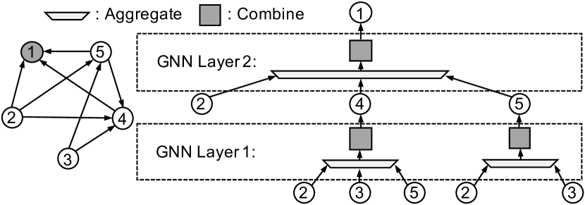
Figure 1. 2-layer GNN training on Node 1

GNN Training. A GNN operates on graph-structured data, where each node has its own feature vector. GNNs aim to produce a quality embedding for each node in the graph capturing its neighborhood information on top of its own feature. These embeddings may be used for various downstream tasks such as node classification and link prediction. To obtain the embedding of a node, GNN takes the feature vectors of not only the target node for embedding computation, which is called seed node, but also its k-hop in-neighbors as input. Each layer in GNN is responsible for synthesizing feature information of the nodes at each hop, which means that k-layer GNN is able to reflect up to k-hop in-neighbors (Defferrard et al., 2016; Kipf and Welling, 2017).

Each layer of GNN consists of two main steps: Aggregate and Combine. The embedding of node $v$ after the $i$th layer, denoted as $h^{i}_{v}$, is computed as the following:

(1) $$h^{i}_{v}=\texttt{Combine}(\texttt{Aggregate}(\left\{h^{i-1}_{u}\mid u\in N(v)\right\}))$$

$N(v)$ denotes the neighbor set of node $v$. In Aggregate step, the features of the incoming nodes are aggregated into a single vector. While popular options for aggregation functions are simple operations like mean, max and sum, more sophisticated aggregation functions are also drawing attention (Veličković et al., 2018). The aggregated feature then goes through Combine step which is essentially a fully connected (FC) layer with a non-linear function. Figure 1 illustrates this process with an example of a 2-layer GNN training on Node $1$.

Neighborhood Sampling.

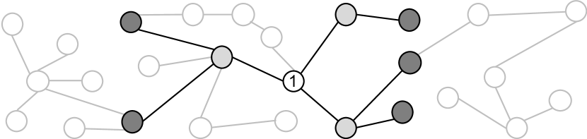
Figure 2. Sampling for a 2-layer GNN (sampling size = (3,2), batch size = 1)

The inter-node dependence of training data poses a unique challenge to GNN training. Even if we use small batch size, the training cost for each batch can still be quite high because collecting $k$-hop in-neighbors leads to exponential growth of memory footprint. Neighborhood sampling is a popular technique for this neighborhood explosion problem. Instead of sampling $k$-hop in-neighbors of seed nodes, sampling algorithms select only a subset of them. One representative work is GraphSAGE (Hamilton et al., 2017), which randomly samples only a predefined number of in-neighbors at each aggregation step. Figure 2 shows an example with a 2-hop computational graph for Node $1$ being sampled. The sampling size in this example is (3,2) which means that it selects (at most) three among the neighbor nodes connected to the target node (Node $1$) and (at most) two are selected for each of the previously selected nodes. Its variants differ in several aspects of sampling function design like the granularity of sampling operation or the choice of probability distribution for sampling (Chen et al., 2018b; Cong et al., 2020; Ying et al., 2018; Chen et al., 2018a). In practice, it is not usual to go beyond three layers, and popular choices of sampling size for GraphSAGE are (25, 10), (10, 10, 10), and (15, 10, 5) (Min et al., 2021).

2.2. GNN Training System

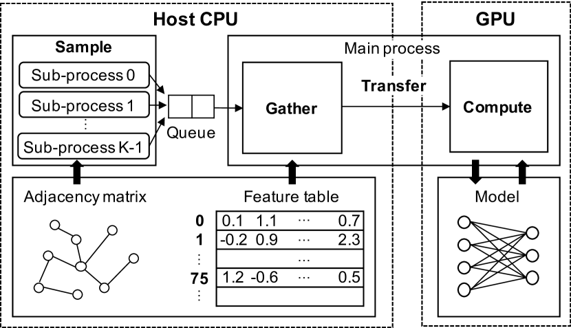
Figure 3. Overview of conventional GNN training system

The state-of-the-art DNN frameworks (Wang et al., 2019; Fey and Lenssen, 2019) employ a mixed CPU-GPU training system, where CPU stores the graph data and is in charge of data preparation, whereas GPU executes the core GNN operations, i.e., aggregate and combine. GPU memory capacity is often fairly limited to store the graph data, while the massive parallelism of GPU is key to accelerating GNN computations. Figure 3 visualizes a typical process of mixed CPU-GPU training of GNN which consists of four steps: (1) sample, (2) gather, (3) transfer, and (4) compute. At every iteration, seed nodes for a single batch as well as their neighbors are extracted by traversing the graph structure (i.e., adjacency matrix) (sample). The adjacency matrix is usually stored in the compressed sparse column (CSC) format as it allows fast access to in-neighbors of each node. Then, the sparsely located feature vectors of the sampled nodes are collected into a contiguous buffer (gather), which is transferred to GPU over PCIe interface (transfer). Lastly, GPU performs forward/backward propagation to compute gradients and updates the parameters (compute). Since sampling operation is often memory-intensive, it is common to spawn multiple sub-processes to increase the sampling throughput. Each sub-process performs a sampling job for a batch, and puts the result into a shared queue. The main process fetches the sampling result from the shared queue and executes the remaining jobs, i.e., gather, transfer, and compute.

2.3. Disk-based GNN Training

Need for Disk-based GNN Training. Although the size of the largest publicly available GNN dataset, ogbn-papers100M (Hu et al., 2021a), is around 100GB, companies reportedly operate on much larger internal datasets that have hundreds of millions or even billions of nodes and tens of billions of edges (Yang, 2019; Zhang et al., 2020). For these datasets, the size of both node feature table and adjacency matrix may reach several hundreds of GBs or even a few TBs, often exceeding the memory capacity of a single node. Distributed training which partitions the graph dataset into multiple nodes in a cluster is a popular solution. However, scaling-out is not necessarily the most cost-effective solution to scale memory capacity (Zhao et al., 2015). In this case, instead of adhering to in-memory processing, leveraging high-performance storage devices like NVMe SSDs as memory extension can be a promising direction owing to its large capacity and hence cost efficiency (Lee et al., 2021).

Bottleneck Analysis. However, it is still difficult to achieve high throughput on an SSD-based GNN training system. SSD operates as a block device where data is transferred in a 4KB chunk while sample and gather usually consist of fine-grained random accesses whose size ranges from tens to hundreds of bytes. Such a coarse access granularity combined with its relatively low bandwidth results in huge I/O penalty. In fact, we have profiled the execution time of SSD-based GNN training. We have trained GraphSAGE with a sampling size of (10,10,10) on a 8-core Intel Xeon CPU with 64GB memory and an NVIDIA V100 GPU equipped with 16GB HBM2 memory. We pipelined the execution of not only sample but also gather with the CUDA operations (transfer and compute) by creating a separate thread for gather. Two large-scale graph datasets whose size of both adjacency matrix and feature table far exceed the host memory capacity are synthetically generated by extending the real world datasets (ogbn-papers100M, ogbn-products) (Lee et al., 2021). We denote ogbn-papers100M and ogbn-products by papers and products, respectively, in following figures. The graph dataset (i.e., adjacency matrix and feature table) is memory-mapped by mmap syscall. The details on the setup and the datasets are elaborated in Section 5.1.

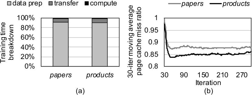
Figure 4. (a) Training time breakdown and (b) OS page cache miss ratio of SSD-based GNN training system with memory-mapped graph dataset

Figure 4(a) shows the training time breakdown, and Figure 4(b) the page cache miss ratio of the GNN training program over time by measuring a 30-iteration moving average. For both datasets, more than 90% of training time is stalled by data preparation (i.e., sample and gather). In addition, the page cache miss ratio is fairly high. The miss ratio rapidly drops in the beginning as the page cache gets filled, but it soon stabilizes at 85-90%. This implies that I/O is the bottleneck, and thus it is important to reduce the number of I/Os in sample and gather. Among the two, especially gather needs to be optimized. This is because the number of I/Os is usually several-fold higher in gather than in sample. Assuming a 3-layer model, all the sampled 3-hop neighbors of the seed nodes should be gathered for each iteration. Meanwhile, examining neighborhood information of the 2-hop neighbors of the seed nodes is enough to sample the 3-hop neighbors. In fact, in our experiments, the number of I/O requests made in gather is reported to be $8.13\times$ and $9.75\times$ higher than in sample for ogbn-papers100M and ogbn-products, respectively.

Challenge 1. Sub-optimal In-memory Cache. As OS page cache, which simply keeps the recently accessed pages, is shown to be ineffective for GNN training, application-specific in-memory cache can be a viable alternative. There have been proposals to cache part of a graph dataset considering the access pattern of GNN training. Although they usually assume different training scenarios and target to optimize different types of data movement like communications among cluster machines or between CPU and GPU, not disk I/O, their spirits can be extended for the SSD-based training system.

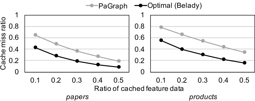
Figure 5. Cache miss ratio of PaGraph and optimal cache with different cache sizes

For example, PaGraph (Lin et al., 2020), a state-of-the-art cache design for feature table, caches feature vectors of nodes with a descending order of out-neighbor count. While being moderately effective, this design is sub-optimal as it is static and relies on simple heuristics. Figure 5 demonstrates cache miss ratio of PaGraph in gather step for the two datasets compared to the optimal cache miss ratio with different cache sizes. The optimal cache policy is defined by Belady’s cache replacement algorithm, which always evicts data that will not be needed for the longest time in the future (Belady, 1966). The gap from the optimal indicates that there leaves much room for improvement.

Challenge 2. Sub-optimal Pipeline.

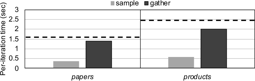
Figure 6. Per-iteration time of stand-alone execution of sample and gather compared to that of pipelined execution of the two operations (represented by dotted line)

While the two data preparation operations of GNN, sample and gather, are pipelined in the conventional training system, they are not actually an ideal pair for parallel execution especially for disk-based training. This is because they are both I/O intensive operations whose parallel execution can incur resource contention. Under ideal pipelined execution, the time required for data preparation should be determined by the one which takes more time. However, this is not the case as shown in Figure 6. There exists a considerable gap between the stand-alone execution time of the longer operation (gather) and the pipelined execution time (dotted line). This indicates that the conventional pipeline has very limited performance benefit.

3. Ginex Design

Ginex is a system for efficient training of a very large GNN dataset by using SSD as a memory extension. Specifically, Ginex targets dataset whose adjacency matrix as well as feature table do not fit in CPU memory. Ginex reduces I/O traffic from the two I/O intensive operations, sample and gather, by effectively utilizing the main memory space as application-specific in-memory cache. Especially for gather, Ginex provides the provably optimal caching mechanism. The rearrangement of the training pipeline, inspired by the inspector-executor model (Mirchandaney et al., 1991; Strout et al., 2018) in compiler optimization, enables this optimal caching, which would otherwise be infeasible.

The rest of this section is organized as follows. In Section 3.1, we overview the training pipeline of Ginex. Section 3.2 explains the Ginex neighbor cache (i.e., cache for sample), while Section 3.3 and Section 3.4 explain the Ginex feature cache (i.e., cache for gather). Section 3.5 provides a guideline for configuring Ginex’s parameters.

3.1. Ginex Training Pipeline

Overview.

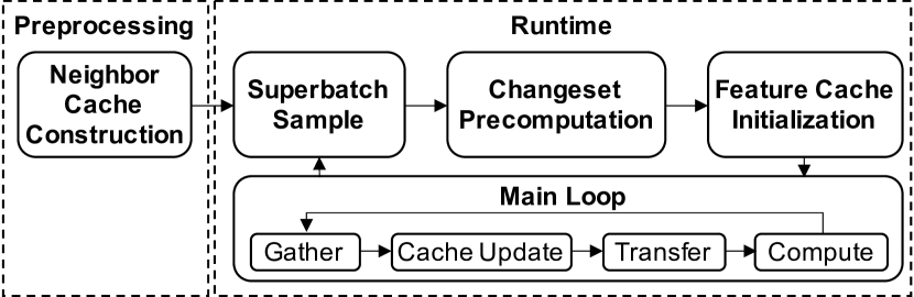
Figure 7. Ginex training pipeline overview

Figure 7 depicts a high-level overview of Ginex’s training pipeline. After a short preprocessing procedure, Ginex starts training by iterating the following four stages: superbatch sample, changeset precomputation, feature cache initialization, and main loop. In the superbatch sample stage, Ginex performs sampling for a predefined number of batches, which we call superbatch, all at once. With the sampling results, Ginex finds all the information necessary to manage the feature cache for the following gather operations in the changeset precomputation stage. Specifically, in this stage, Ginex determines (i) which feature vectors to prefetch into the feature cache at initialization, and (ii) which feature vectors to insert and which ones to evict from the feature cache (i.e., changeset) at each iteration. After a short transition stage for the feature cache initialization, Ginex completes the remaining tasks including gather in the main loop stage.

Inspector-Executor Execution Model. The inspector-executor execution model is originally introduced to enable runtime parallelization and scheduling optimization of loops (Mirchandaney et al., 1991; Strout et al., 2018). An inspector procedure runs ahead of the executor to collect information that is available only at runtime, such as data dependencies among array elements. The executor is an optimized version of the original application that utilizes this runtime information to optimize data layout, iteration schedule, and so on. Ginex embraces this execution paradigm to improve the efficiency of in-memory caching for GNN training. In particular, the first two runtime stages, superbatch sample and changeset precomputation, correspond to the inspector, and the main loop stage to the executor. By running ahead the sample operation for the entire superbatch, Ginex collects complete information about the nodes to be accessed later in the gather stage, thus enabling optimal management of the feature cache.

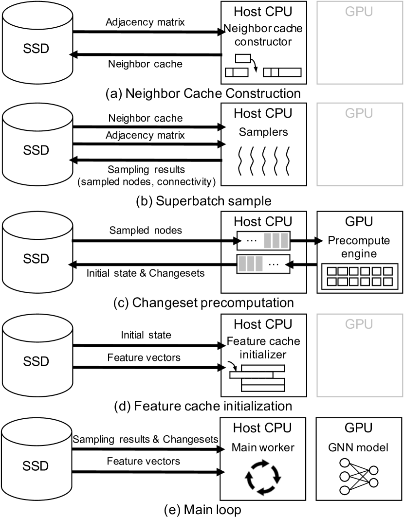
Figure 8. Illustration of Ginex training pipeline stages

Neighbor Cache Construction. Figure 8(a) shows this process. Unlike the feature cache which dynamically manages its data, Ginex uses a static neighbor cache for the whole training process. Therefore, Ginex constructs the neighbor cache with a given size during offline preprocessing time. To make the neighbor cache, Ginex examines the graph structure (i.e., adjacency matrix) and picks out important nodes whose list of in-neighbors would be cached. The criterion for selecting important nodes will be discussed in Section 3.2. After finishing this construction, Ginex saves the neighbor cache by dumping it to SSD, which would be loaded at the beginning of each of the following superbatch sample stages. This avoids the repeated cost of constructing the neighbor cache, which may include a large number of random reads of which sizes are usually only a few tens or hundreds of bytes.

Superbatch Sample. Figure 8(b) depicts the first stage of Ginex runtime, superbatch sample. In this stage, Ginex first loads the neighbor cache which has been constructed and stored in SSD during preprocessing. Basically, all memory space except the working buffer for sampling processes can be used for the neighbor cache. After then, multiple sub-processes are launched and sampling is started for as many batches as the superbatch size, $S$. When accessing the neighbor information during the sampling process, Ginex first looks up the cache and only reads the data from SSD when it is not present in the cache. The sampling results of a superbatch are then written to SSD. Usually, a sampling for each batch results in two types of data. One is $ids$ which is an 1-D list of all the sampled nodes’ IDs. The other is $adj$, a data structure that describes the connectivity among the sampled nodes. Ginex stores these two data in separate files annotated with the batch index. In total, $2\times S$ files ($ids\_0,ids\_1,...$ $,ids\_(S-1),adj\_0,adj\_1,...$ $,adj\_(S-1)$) are generated. The size of each file varies depending on the sampling size, the batch size, and the characteristics of the dataset, but usually ranges from several hundred KB to a few MB.

Changeset Precomputation. Figure 8(c) shows the third stage of Ginex runtime, changeset precomputation. Instead of computing a changeset (i.e., which features to insert into and evict from the feature cache) every time Ginex performs gather in main loop stage, Ginex precomputes all the changesets beforehand by examining the list of sampled nodes ($ids$ files). This is to accelerate the changeset computation in batch on GPU. It is difficult to allocate enough memory and computation resources of GPU for the changeset computation in main loop stage as it involves GPU computation. As the total size of $ids$ files may exceed the GPU memory capacity, each $ids$ file is first loaded on the CPU memory and then streamed into GPU when needed. The results of the changeset precomputation are sent back to CPU, and are stored in SSD also by streaming. Besides the changesets, a list of the feature vectors to prefetch into the cache at initialization is also obtained at this stage. Specifically, $S+1$ files are generated in this step including one for cache initialization ($init$) and the others for cache update for every $S$ iterations ($update\_0,update\_1,...$ $,update\_(S-1)$).

Feature Cache Initialization. Figure 8(d) shows this process. In this step, Ginex reads the previously created $init$ file from SSD and constructs the feature cache. This process includes reading feature vectors of the nodes specified in $init$ file as well as building an address table that will be used for cache look-up.

Main Loop. Figure 8(e) illustrates this stage. This stage is where all the remaining GNN training operations for each batch (gather, transfer, and compute) are performed iteratively. In addition, Ginex performs one more operation, cache update, in between. At each iteration, Ginex reads a set of $ids$, $adj$ and $update$ files from SSD in the order of the batch index. Then, Ginex makes batch input by gathering feature vectors according to the $ids$ file from either the cache or SSD, and updates the cache as indicated in the $update$ file. Lastly, the batch input and $adj$ are transferred to GPU in order to perform forward and backward pass as well as model update in the same way as the conventional GNN training system.

Superbatch-level Pipeline.

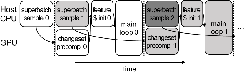
Figure 9. Superbatch-level pipeline of Ginex

While the four runtime stages for the same superbatch should be serialized, the jobs from different superbatches can be pipelined. Taking this opportunity, Ginex performs the jobs for different superbatches in a pipelined manner in order to improve end-to-end performance. Specifically, changeset precomputation for each superbatch is executed in parallel with the superbatch sample of the next superbatch. superbatch sample runs on CPU, while changeset precomputation mainly consumes GPU resources except the I/O overhead of streaming $ids$ files and the changeset precomputation results. This makes these two stages apposite candidates of parallel execution. Figure 9 visualizes Ginex’s superbatch-level pipeline. While the storage overhead of runtime files is doubled as a result of pipelining, it successfully hides most of the changeset precomputation overhead.

Implications on Training Quality. The new training schedule of Ginex has no impact on training quality, as it only changes the execution order of operations which do not have any dependence with each other. It does not require any change in sampling algorithm or GNN model computation.

3.2. Neighbor Cache

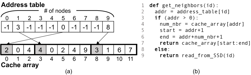
Figure 10. (a) Ginex neighbor cache structure and (b) pseudocode for its operation

Neighbor Cache Policy. By caching part of the adjacency matrix in memory, Ginex reduces the number of storage I/Os during sampling. In other words, Ginex keeps the direct in-neighbors of some important nodes in its neighbor cache in superbatch sample stage. To select important nodes, Ginex adopts a simple metric introduced in Aligraph (Yang, 2019) which quantifies the trade-off between cost and benefit of caching neighbors of each node in a heuristic way. Specifically, the metric is defined as the ratio between the number of out-neighbors and in-neighbors, as access frequency (benefit) may be roughly proportional to the number of out-neighbors while the cache space overhead (cost) is proportional to the number of in-neighbors. Meanwhile, Aligraph uses the ratio between the number of $k$-hop in-neighbors and out-neighbors, as it caches $k$-hop neighbors ($k\geq 2$). However, as Ginex caches direct neighbors, the ratio between the number of direct in-neighbors and out-neighbors is used as the importance metric for Ginex.

Neighbor Cache Structure. Figure 10(a) shows the structure of Ginex’s neighbor cache. Taking a node ID as input, the neighbor cache should return a list of the target node’s neighbors if it is cached, or a cache miss signal if not. For this purpose, Ginex’s neighbor cache uses direct addressing. It has an $address\_table$, an 1-D array which has as many elements as the total number of nodes. Each element of the $address\_table$ contains an index to look up in the $cache\_array$. A $cache\_array$ is an 1-D array that keeps the neighbor information of the cached nodes for the corresponding node for a cache hit, or an arbitrary negative number (e.g., -1) for a cache miss. Such direct addressing makes its lookup very fast, clearly an $O(1)$ operation, but may incur space overhead owing to the redundancy in its $address\_table$ design. Still, it is affordable as the space overhead of having only a single value for every node is several orders of magnitude smaller than having the whole dataset.

Since each node has a different number of neighbors, the elements of the $cache\_array$ pointed by the $address\_table$ contain the number of neighbors for the corresponding node, and the actual IDs of the neighbors (listed from the next element). For example, in Figure 10(a), the neighbor information of Node $1$, $5$ and $9$ are cached since their entries are non-negative. As $address\_table[1]$ is 3, it means that the neighbor information of Node 1 starts from $cache\_array[3]$. Since $cache\_array[3]$ is 4, the number of neighbors of Node 1 is 4, and the IDs of its neighbors are listed in 4 consecutive entries, i.e., $cache\_array[4]$ through $cache\_array[7]$. Figure 10(b) presents a pseudocode that returns neighbors of a given node using the neighbor cache. Three memory accesses (Line 2, 4, and 7) are needed to fetch the neighbor list from the cache.

3.3. Feature Cache

Feature Cache Policy. The feature cache in Ginex adopts the provably optimal Belady’s algorithm (Belady, 1966). Belady’s cache replacement algorithm evicts data with the highest reuse distance at every timestep. Reuse distance for the data is defined as the time until the next access to it. This policy is basically an oracle policy which requires the knowledge of future data accesses, so is infeasible in most cases. In practical settings, only attempts to approximate Belady’s cache replacement algorithm have been made (Liu et al., 2020; Jain and Lin, 2016; Shi et al., 2019).

However, it is possible for Ginex to implement this optimal caching mechanism for feature vectors in the exact form as the sampling results for the whole superbatch are available at the time of gather. Therefore, Ginex’s feature cache dynamically updates its data following Belady’s cache replacement algorithm. Specifically, when updating the cache data at each iteration, the feature cache prioritizes the feature vectors that would be accessed in earlier iterations within the current superbatch. Initially, to minimize cold misses, Ginex prefetches the feature vectors that appear at the first few iterations into the feature cache until it gets full.

Feature Cache Structure. Ginex’s feature cache also uses the same direct addressing as the neighbor cache. Meanwhile, the size of the feature vector is same for all nodes, so the cache array of the feature vector is a simple 2-D array whose row length equals the feature vector size. In the case of a cache hit, the corresponding element in the address table contains the row index of the cache array to look up. In the case of a cache miss, identical to the case in the neighbor cache, the corresponding element in the address table contains an arbitrary negative value (e.g., -1).

Feature Cache Update. The changeset precomputation results in three 1-D lists for each iteration which are $in\_ids$, $out\_ids$ and $in\_positions$. $in\_ids$ and $out\_ids$ specifiy the IDs of the nodes to be inserted and evicted, respectively. $in\_positions$ specifies positions of the nodes in $in\_ids$ within a batch input. The batch input refers to the feature vectors collected in a contiguous buffer by gather operation, which is to be transferred to GPU.

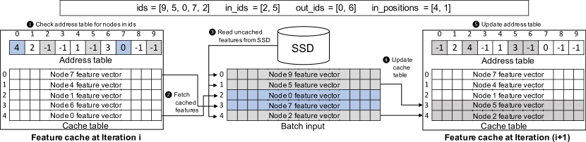
Figure 11. Example of cache update followed by gather

Figure 11 shows the process of cache update followed by gather using an example. This example shows the change of feature cache when moving on to Iteration ($i+1$) from Iteration $i$. In this example, the total number of nodes are 10, and five of them are cached (Node $0$, $1$, $4$, $6$, and $7$). $ids$ refers to the sampled node IDs, while $in\_ids$, $out\_ids$ and $in\_positions$ are cache update information for the current iteration. For gather, Ginex first checks $address\_table$ for the nodes in $ids$ . The feature vectors of the nodes present in the cache (Node $0$ and Node $7$) are fetched from the cache , while the others are read from SSD to make the batch input. Note that the ordering of the feature vectors within the batch input is the same as $ids$. After the batch input is made, Ginex performs cache update by referring to $in\_ids$, $out\_ids$ and $in\_positions$. In the figure, $in\_ids$ and $out\_ids$ indicate that the feature vectors of Node $2$ and Node $5$ should replace the cache lines occupied by the feature vectors of Node $0$ and $6$. As the feature vectors of Node $2$ and $5$, which are newly loaded from SSD, are buffered in the batch input, Ginex locates these two vectors with $in\_positions$. Then, Ginex puts these vectors into the cache lines originally holding the feature vectors of Node $0$ and Node $6$, whose address can be found by checking $address\_table$ . Lastly, Ginex updates $address\_table$ as well , and cache update for Iteration $i$ ends.

3.4. Changeset Precomputation Algorithm

Problem Formulation. Computing the changeset is no more than simulating the cache state (i.e., node IDs present in the cache) of every iteration as the changeset can be obtained by comparing the difference between the two consecutive cache states. In other words, it is to solve the following recurrence relation for $i$ from $0$ to $S-2$, where $S$ is the superbatch size.

$$C_{i+1}=f_{Belady}(union(C_{i},ids\_i))$$

where $C_{i}$ is the cache state at Iteration $i$. The initial cache state ($C_{0}$) and the lists of node IDs that would be accessed at each iteration of superbatch ($ids\_0,ids\_1,...,ids\_(S-2)$) are given as inputs. $f_{Belady}$ is a function that selects the elements in the given list, prioritizing those that are to be accessed earlier than others, as many as the number of cache entries. As all the feature vectors of the nodes in $ids\_i$ are loaded onto memory at Iteration $i$, the union of $C_{i}$ and $ids\_i$ are potential candidates to be included in $C_{(}{i+1)}$.

The main challenge in solving $f_{Belady}$ is to find out the next accessed iterations of the given nodes in $union(C_{i},ids\_i$) at each iteration. Here, we denote the iteration that the node is to be accessed next by the node’s next accessed iteration. A straightforward approach is to examine all the future data access traces ($ids\_({i+1})$, $ids\_({i+2})$, …) in order to check in which iteration the feature vector of each node in $union(C_{i},ids\_i)$ would be accessed next time. Such a naïve approach, however, results in the worst case complexity of $O(S^{2})$ whose cost can be substantial as we increase the superbatch size. To prevent the changeset precomputation stage from being the major bottleneck, we propose an efficient algorithm with just an $O(S)$ complexity.

Sketch of Our Algorithm. Ginex solves the problem with only three passes over the access traces. With the first two passes, Ginex builds a data structure specially designed for the incremental tracking of each node’s next accessed iteration. With this data structure, in the last pass, Ginex simulates a whole sequence of cache states. The following paragraphs discuss how this data structure looks like and operates as well as how the end-to-end algorithm works in details.

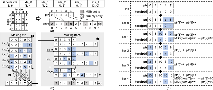
Figure 12. Example for next accessed iteration tracking of Ginex. (a) shows data structures for the tracking while (b) shows the process of making it. (c) shows how Ginex tracks the next accessed iteration.

⬇

1# num_entries: the number of cache entries

2# ids_list: the list of data access traces ([ids_0, ids_1, …, ids_S-1]) stored in SSD

3

4current_cache_state = initial_cache_state

5for ids in ids_list:

6 incoming_ids = Load(ids)

7

8 ptr[incoming_ids] += 1

9 for id in incoming_ids where MSB(iters[ptr[id]]) is set:

10 ptr[id] = len(iters)-1

11

12 candidates = Union(current_cache_state, incoming_ids)

13 next_access_iters = iters[ptr[candidates]]

14

15 # select N elements in candidates with the smallest next accessed iteration

16 new_cache_state = TopKSmallest(candidates, next_access_iters, num_entries)

17

18 # find relative complement of new_cache_state & current_cache_state with respect to each other

19 in_ids = new_cache_state - current_cache_state

20 out_ids = current_cache_state - new_cache_state

21 in_positions = IndexOf(in_ids, incoming_ids)

22

23 Save((in_ids, out_ids, in_positions))

Figure 13. Pseudocode for end-to-end changeset precomputation process

Tracking Next Accessed Iteration. Figure 12(a) shows the data structure that Ginex utilizes for tracking next accessed iterations of nodes with a simple example, where both the number of nodes and the superbatch size are five. We assume that two nodes are sampled for each iteration, which means that the length of each $ids$ is two. Conceptually, the access traces ($ids\_0,ids\_1,...,ids\_4$) can be represented as a binary matrix where each row corresponds to each node while each column corresponds to each iteration. ($i$,$j$) is set to $1$ if Node $i$ appears at Iteration $j$, or $0$ otherwise. What Ginex maintains for next accessed iteration tracking is a sort of CSR-format of this matrix which consists of two arrays: iters and ptr. iters lists accessed iterations of each node in sequence from Node $0$. Each node’s accessed iterations are kept in sorted order. ptr array has elements as many as the number of nodes each of which points to the start of the corresponding node’s accessed iterations in iters. For example, ptr[$3$] is $4$, which means that from iters[$4$], the iterations in which Node $3$ appears ($0$, $2$, $4$) are listed in order. The most significant bit (MSB) of the elements in iters pointed by ptr is set to $1$ and a dummy entry whose value is set to the maximum value for a given datatype is appended at the end of iters.

The construction of this data structure requires two passes over the access traces. Figure 12(b) shows this process. In the first pass, Ginex counts the number of appearances of each node . Then, Ginex performs cumulative sum over the count results and completes making ptr by inserting zero value in the front and deleting the last element . In the second pass, Ginex makes iters with a guide of ptr . At Iteration $0$, Node $3$ and Node $4$ are accessed. So Ginex sets 0 for the elements pointed by ptr[$3$] ($4$) and ptr[$4$] ($7$), then increments ptr[$3$] and ptr[$4$] by one. This process is repeated for the remaining iterations. At last, Ginex restores ptr by a simple shift and completes iters construction by appending a dummy entry and setting MSBs for elements pointed by ptr to 1 .

Using these two arrays, Ginex can track next accessed iteration of the nodes with a single additional pass over the access traces, which completes the cache state simulation. Ginex updates ptr for each iteration in a way that it can always find out the next accessed iterations of all nodes by looking at the elements in iters pointed by ptr. Figure 12(c) shows this process with the same example as before. In the figure, ptr and a subset of of iters pointed by ptr (iters[ptr]), which would indicate the next accessed iteration of the nodes, are shown at initialization and each iteration. Note that Ginex does not maintain iters[ptr] in fact but only looks up a necessary part on demand. We show the change of iters[ptr] along with ptr just for demonstration. At initialization, iters[ptr] denotes the first accessed iteration of the nodes. When simulating each iteration, ptr values for the accessed nodes are incremented by $1$. This is natural as the next accessed iteration of the currently accessed nodes should be updated. For example. at Iteration $0$ in the figure, ptr[$3$] and ptr[$4$] are incremented by $1$. If the MSB of the iters element pointed by the updated ptr value is $1$, however, that ptr value is set to point the last element of iters, which is the dummy entry. This is to regard the next accessed iteration of such a node which would not appear again in the future as a very large value. For example, at Iteration $1$ in the figure, ptr[$2$] is set to $10$, the index of the dummy entry in iters, since the MSB of iters[$4$] is set to $1$. The same process is repeated until the end of the simulation.

End-to-end Algorithm. Figure 13 is a pseudocode that shows the end-to-end process of the changeset precomputation which eventually produces the three lists ($in\_ids$, $out\_ids$, and $in\_positions$) for each iteration. For each iteration, the data access trace for each iteration (incoming_ids) originally stored in SSD is loaded into GPU in order (Line 6). The ptr is updated to remain up-to-date (Line 8-10). With the updated ptr, the next accessed iterations are obtained for the candidates which is the union between the IDs in the current cache and incoming node IDs (Line 12-13). After that, the new cache state is derived by selecting top-num_entries smallest among the next accessed iterations of the candidates (Line 16). By computing the set difference between the new cache state and the current cache state, $in\_ids$ and $out\_ids$ can be obtained (Line 19-20), after which $in\_positions$ is computed by figuring out the positions of each node in $in\_ids$ within incoming_ids. Finally, the three resulting lists are sent back to the host and saved in SSD.

3.5. Configuring Ginex

Superbatch Size. For performance, it is always better to increase the superbatch size. This is because a large superbatch can amortize the cost of switching between superbatch sample and main loop, which includes loading the neighbor cache and initializing the feature cache. This switch cost depends on the cache size and remains constant with respect to the superbatch size. However, it is not possible to increase the superbatch size indefinitely for the following reasons. First, GPU memory size imposes a hard limit on the superbatch size. The amount of GPU memory required to perform the changeset precomputation increases with the superbatch size. However, this is not often the case unless a very large superbatch size (e.g., $10000$) is used. Instead, the storage overhead of runtime files may be a practical factor that limits the superbatch size. One can increase the superbatch size as much as the storage constraint permits. In our evaluation setting, 100GB of runtime files are a good trade-off between the performance and storage overhead (Section 5.3). Since the runtime file size per iteration is relatively constant throughout the training process, one can readily approximate the storage overhead via a short offline profiling.

Cache Size. The size of the neighbor cache and the feature cache should be determined before the beginning of the training. Since the peak memory usage at each iteration of superbatch sample and main loop remains stable throughout the training process, we can again determine the cache size by a short offline profiling. We set the cache size by subtracting the peak memory usage at each stage (superbatch sample for the neighbor cache and main loop for the feature cache), and the size of additionally reserved region for memory fluctuations from the total memory size.

4. Implementation

We have implemented Ginex by extending PyTorch Geometric (PyG) (Fey and Lenssen, 2019), a popular open-source framework for GNN training built upon PyTorch (Paszke et al., 2019), as follows. First, we have created new extensions for sampling and gathering to support the user-level in-memory cache. Specifically for sampling, we have modified PyTorch Sparse C++ backend which PyG calls for sampling-related operations. We use pread syscall with O_DIRECT flag to bypass OS page cache when accessing to graph data stored in SSD. Second, we have made an extension also for cache updates. To copy sparsely located data in a tensor to the specified locations of another tensor, PyTorch tensor indexing API requires to collect the data from the source tensor in a contiguous buffer first and then scatter them to the destination tensor, which incurs redundant memcpy. Our extension eliminates such waste by directly copying data from the source to the destination. This process is parallelized by OpenMP. Third, we have modified NeighborSampler class of PyG in a way that it stores the sampling results to disk in order instead of putting them into a shared queue. To load the saved files at each iteration of the main loop stage, we use a custom lightweight multi-threaded dataloader. Lastly, we take advantage of highly-optimized CUDA kernels of PyTorch for changeset precomputation.

5. Evaluation

5.1. Methodology

System Configurations. Table 1 summarizes our system configurations. We evaluate Ginex on a Gigabyte R281-3C2 server with an 8-core CPU (16 logical cores with hyper-threading), an NVIDIA V100 GPU, and a Samsung PM1725B NVMe SSD.

Table 1. System configurations

CPU Intel Xeon Gold 6244 CPU 8-core @ 3.60 GHz GPU NVIDIA Tesla V100 16GB PCIe Memory Samsung DDR4-2666 64GB (32GB $\times{}$ 2) Storage Samsung PM1725b 8TB PCIe Gen3 8-lane S/W Ubuntu 18.04.5 & CUDA 11.4 & Python 3.6.9 & PyTorch 1.9

Model and Dataset. We use 3-layer GraphSAGE (Hamilton et al., 2017) and 2-layer GCN (Kipf and Welling, 2017) for evaluation. Both models have a hidden dimension of 256. For GraphSage, we set a sampling size to (10,10,10). By default, we set batch size to 1000. To evaluate Ginex on a billion-scale graph, we scale four real-world datasets: ogbn-papers100M (papers) (Hu et al., 2021a), ogbn-products (products) (Hu et al., 2021a), com-friendster (Friendster) (Leskovec and Krevl, 2014), and twitter-2010 (Twitter) (Leskovec and Krevl, 2014) following the methodology in  (Lee et al., 2021). Specifically, we use a graph expansion technique (Belletti et al., 2019), which adapts Kronecker graph theory (Leskovec et al., 2010) to preserve innate distributions of recipe graphs like power-law degree distribution and community structure. We then randomly choose 10% of the nodes to serve as a training set. Even with this split of the dataset, the working set may contain the feature vectors of the whole dataset as GNN training takes the feature vectors of not only the nodes in the training set but also their $k$-hop neighbors as input. By default, we set the feature dimension of all datasets to 256. The whole datasets are assumed to be stored in SSD during training except the pointer array in a CSC-formatted adjacency matrix. While the pointer array takes only about a few GBs, it is very frequently accessed during the sample stage. Thus, we keep it in memory when performing sample. Table 2 summarizes the key features of the datasets.

Table 2. Graph datasets

Original Large-scale Dataset nodes edges nodes edges size ogbn-papers100M 111.06M 1.62B 444.24M 14.24B 569GB ogbn-products 2.45M 61.86M 220.41M 20.24B 388GB com-friendster 65.61M 1.81B 262.43M 15.48B 393GB twitter-2010 41.65M 1.47B 208.26M 14.05B 326GB

Comparison Baselines. We compare Ginex with two baselines: PyG+, Ali+PG. PyG+ refers to the PyG framework modified to support disk-based GNN training over a memory-mapped graph dataset. It follows the conventional GNN training pipeline explained in Section 2.2. We used memmap function of NumPy (Harris et al., 2020) to create a memory-map to an array stored in a binary file and converted the memory-mapped array into a PyTorch tensor. As an optimization for PyG+, we disable the readahead feature, which only degrades the performance of GNN training as it incurs a large number of random disk accesses. In addition, we set the number of threads to use for I/O intensive operations like gather, more than twice the number of cores to better utilize the disk bandwidth instead of using the default PyTorch setting which is the number of physical cores. Ali+PG is PyG+ augmented by an application-specific in-memory caching mechanism for sample and gather. Specifically, an Aligraph-style cache (Yang, 2019) is used for the neighbor cache and a PaGraph-style (Lin et al., 2020) cache is used for the feature cache. For Ali+PG, we tune the sizing of the two caches by splitting the available memory space on the ratio of 0:100, 25:75, 50:50, 75:25, and 100:0 for the neighbor cache and the feature cache, and report the one that yields the best performance. Ali+PG represents a strong baseline by integrating two state-of-the-art caching techniques. For all schemes, we overlap the CUDA operations (transfer, compute) on GPU with the CPU operations to reduce data stalls. For each data point we report the mean of three measurements with an error bar.

5.2. Overall Performance

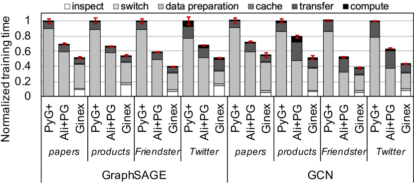
Figure 14. Normalized training time breakdown of PyG+, Ali+PG, and Ginex. Smaller is better.

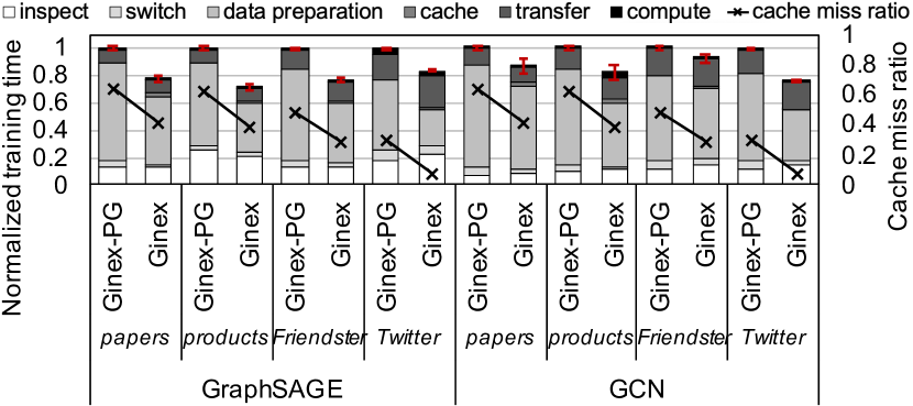
Figure 15. Normalized training time breakdown of Ginex-PG and Ginex

We first measure and break down the training time of PyG+, Ali+PG and Ginex for the four datasets. For GraphSAGE, the superbatch size of Ginex is set to 3300, 2100, 3600, and 6400 for papers, products, Friendster, and Twitter. For GCN, we set the superbatch size of Ginex to 2500, 300, 900, and 900, respectively. We derive these values via the offline profiling-based heuristic in Section 3.5. The actual size of runtime files falls very close to our target (100 GB) within 3%.

Figure 14 shows the results. The training time of PyG+ and Ali+PG can be broken down into three components: data preparation, transfer, and compute. Data preparation time refers to the amount of time that the CUDA operations are stalled either by sample or gather. Meanwhile, the training time of Ginex has three more components: inspect, switch, and cache update. Inspect time refers to the time consumed for the pipelined execution of superbatch sample and changeset precomputation. In all cases the time for changeset precomputation completely hidden by superbatch sample, and the inspect time is equal to the time for superbatch sample. Switch time is the time spent for initializing the feature cache. For Ginex, data preparation time includes not the time for sample but that for gather and runtime file loading.

For all workloads Ginex demonstrates the superior performance. For GraphSAGE the speedups of Ginex range 1.86-2.50$\times$ over PyG+ and 1.23-1.47$\times$ over Ali+PG. For GCN Ginex is 1.83-2.67$\times$ and 1.28-1.57$\times$ faster than PyG+ and Ali+PG, respectively. This performance gains are attributed to the optimal caching scheme for gather outweighing the cost for it. The overhead of the serialization of sample and gather is shown to be insignificant as expected. The switch time and cache update time also account for a minor portion (less than 10%). All these benefits come with a moderate storage cost of about 145 GB (for runtime files and neighbor cache), which is less than a half of the smallest dataset being used.

5.3. Impact of Optimal Feature Cache

In Figure 15, we evaluate Ginex with its cache policy replaced by PaGraph (Ginex-PG) to measure the impact of Ginex’s optimal feature cache in isolation. We report the normalized training time and the cache miss ratio. Ginex consistently demonstrates significantly lower miss ratio, which leads to a proportional reduction in data preparation time. The adoption of the optimal feature cache, however, results in a slightly longer inspect time. While the changeset precomputation can be hidden under the superbatch sample, it may slow down superbatch sample as it involves disk I/Os to stream input and output of the changeset precomputation. However, the increase of inspect time is limited to less than 20%, which is small compared to the data preparation time reduction.

5.4. Sensitivity Study

We conduct a sensitivity study with varying four parameters that may affect performance: superbatch size, feature dimension, memory size, and batch size. We only use GraphSAGE for this study.

Impact of Superbatch size.

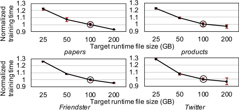
Figure 16. Training time of Ginex normalized to the default superbatch size (circled) on varying superbatch sizes

In Figure 16, we evaluate Ginex with different superbatch sizes to quantify its performance impact. Specifically, we adjust the target runtime file size from 25 GB to 200 GB and report the training time normalized to that of the default setting in which the target runtime file size is 100 GB. Generally, the larger the superbatch size is, the better the performance tends to be. This is mainly because the switch time, which remains constant, is amortized. However, increasing the superbatch size eventually gives diminishing returns beyond a certain point. For example, doubling the runtime file size from 100 GB to 200 GB results in only a marginal decrease of the training time ($7.22\%$, $3.15\%$, $4.81\%$, and $3.16\%$ for the four datasets). Thus, it is an effective heuristic to set the target runtime file size (100GB in our setting) based on the storage capacity constraint as discussed in Section 3.5.

Impact of Feature Dimension.

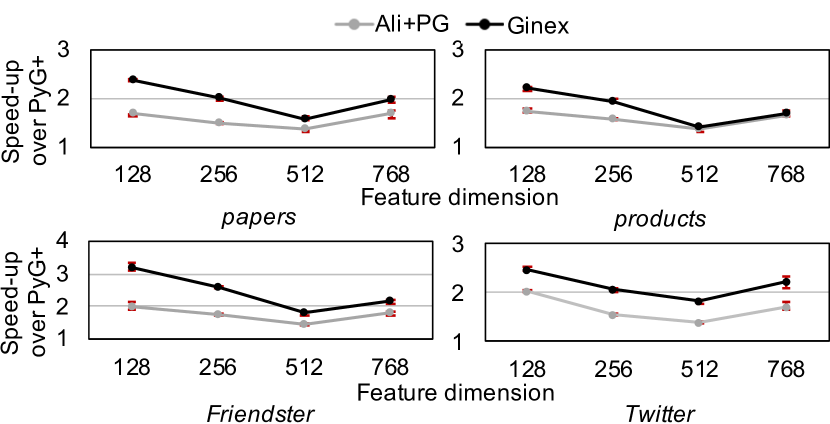
Figure 17. Speedup of Ali+PG and Ginex over PyG+ with varying feature dimensions

In Figure 17, we evaluate the impact of feature dimension on performance. Specifically, we run experiments scaling the feature dimension to $\times 0.5$, $\times 2$ and $\times 3$ of the default setting (256). We report the speedup of Ginex and Ali+PG over PyG+. While Ginex is consistently faster than PyG+ as well as Ali+PG, the degree of its improvement varies with the feature dimension. For the feature dimension of 128, 256 and 512, the higher the feature dimension, the smaller the gap among the three schemes. This can be explained by two factors. First, the relative miss penalty of in-memory cache gets smaller as the feature dimension increases. Regardless of whether the feature dimension is 128, 256, or 512, the miss penalty is the same as a whole 4KB page should be read from SSD. On the other hand, the hit time linearly increases with the feature dimension. Thus, the reduction of the number of cache misses is more critical when the feature dimension is low, which makes the impact of Ginex’s optimal caching more significant. Second, the relative cache size compared to the whole feature table size gets smaller with higher feature dimension. For example, when using a feature dimension of 512 in papers dataset, only about 5% of the whole feature data can be kept in Ginex’s feature cache. In such case, there is usually no significant difference in terms of cache miss ratio between different mechanisms.

Meanwhile, the experimental results with the feature dimension of 768 do not follow the trend discussed above. The gap among the three schemes becomes slightly greater. This is because of the alignment issue. When the feature dimension is 768, the size of each feature vector is 3KB assuming 32-bit floating point format. In this case, a single feature vector may often span two 4KB pages, which means that one should read 8KB in total from SSD to access it. This does not happen when the feature dimension is 128, 256 and 512 as the page size is aligned with the feature vector size. This issue amplifies the miss penalty, thereby making the impact of in-memory caching mechanism more pronounced.

Impact of Memory Size.

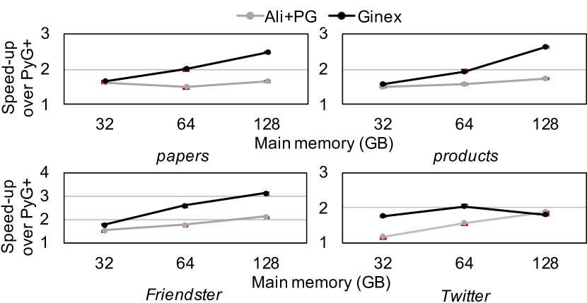
Figure 18. Speedup of Ali+PG and Ginex over PyG+ with varying main memory size

Figure 18 shows the impact of memory size. We scale the memory size to 0.5$\times$ and 2$\times$ of the default size (64 GB). The performance gap between the two caching schemes tends to get narrower as the memory size gets smaller. It is because only about 10 GB of memory can be used for the cache after sparing enough workspace at 32 GB. Too small cache leads to equally poor caching performance for both schemes. Meanwhile, the Twitter dataset demonstrates different trend. Due to the high inter-batch locality, Ginex can achieve substantial performance gains even at 32 GB. However, both schemes are comparable at 128 GB. This is because the caching performance of Ginex already gets saturated with a very low cache miss ratio (<8%) at 64 GB (see Figure 15). Thus, allocation of an additional memory space gives very little benefits to Ginex, whereas Ali+PG gets a substantial boost from it.

Impact of Batch Size.

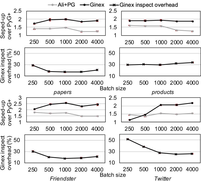
Figure 19. Speedup of Ali+PG and Ginex over PyG+ with varying batch size

Figure 19 shows the impact of batch size. Ginex is consistently faster than Ali+PG except when batch size is very small (e.g., 250). This is because the changeset precomputation overhead of Ginex can be a new bottleneck at a small batch size. As the batch size decreases, the time for changeset computation tends to reduce much more slowly than the other stages which scale almost linearly. Thus, beyond a certain point, the changeset precomputation time is no longer hidden by the superbatch sample stage. However, this behavior manifests at a very low batch size outside the typical range. It is common to use larger batch sizes ($\geq$ 1000) in GNN training (Hu et al., 2021b) for both throughput and accuracy.

5.5. Cost Comparison with Distributed Training

Table 3. Machine configurations on Google Cloud

DistDGL
	Node 0	Node 1-7
Host Processor	24 vCPU	24 vCPU
Host Memory	256 GB	156 GB for Friendster
		128 GB for Twitter
Host Storage	2 TB pd-standard	100 GB pd-standard
GPU	NVIDIA T4 $\times$ 2	NVIDIA T4 $\times$ 2
Network	16 Gbps outbound BW	16 Gbps outbound BW
Hourly Cost (8 Nodes)	$18.83 for Friendster / $17.94 for Twitter
Ginex
Host Processor	12 vCPU
Host Memory	64 GB
Host Storage	375 GB NVMe SSD $\times$ 16
	(Seq. write: 3.12 GB/s, Seq. Read: 6.24 GB/s)
GPU	NVIDIA T4 $\times$ 1
Hourly Cost (1 Node)	$1.36

Table 4. Cost comparison of Ginex and DistDGL

Dataset	Hourly Cost Reduction	Normalized Performance	Normalized Performance/$
Friendster	13.80$\times$	0.20$\times$	2.76$\times$
Twitter	13.15$\times$	0.43$\times$	5.71$\times$

This section presents a case study of comparing the cost efficiency of Ginex with that of DistDGL (Zheng et al., 2021), a popular distributed GNN training system. DistDGL partitions the graph dataset with the min-cut partitioning algorithm (Karypis and Kumar, 1998) and keeps it in memory over a distributed cluster. We set up both Ginex and DistDGL on Google Cloud and report the cost efficiency in terms of performance per dollar on GraphSAGE. We use two datasets, Friendster and Twitter.

Table 3 shows the configurations for DistDGL and Ginex. For DistDGL, we use an 8-node cluster. Each node has two NVIDIA T4 GPUs. This yields a slightly better cost-efficiency than a single-GPU setting. Since Node 0 serves as a master node and thus requires more memory than the others, we equip this node with a larger memory. We have carefully tuned the memory size for the master and worker nodes. Note that the aggregated memory size of the cluster is larger than the dataset size in Table 2. This is because some parts of the graph data are duplicated over multiple nodes for performance, and managing a distributed store consumes additional memory. For Ginex, we use a single node with 64 GB memory, one NVIDIA T4 GPU, and 16 375 GB NVMe SSDs configured with RAID-0.

Table 4 reports the cost efficiency. Ginex achieves 2.76$\times$ and 5.71$\times$ higher cost efficiency than DistDGL in terms of performance per dollar for Friendster and Twitter, respectively. Although the raw training throughput of Ginex is lower than DistDGL, the hourly cost of Ginex is over 13$\times$ lower than DistDGL to make it much more cost effective. The overhead of data distribution over multiple nodes in DistDGL incurs a significant cost when scaling GNN training.

6. Related Work

Scalable Graph Neural Networks. To the best of our knowledge, Ginex is the first to leverage commodity SSDs to scale GNN training. GLIST (Li et al., 2021) also utilizes SSDs to scale GNN but focuses on inference and requires specialized hardware. Instead, most proposals for large-scale GNN training have taken scale-out approaches. ROC (Jia et al., 2020) and NeuGraph (Ma et al., 2019) propose multi-GPU training system for GNN. However, they adopt full-batch training which makes them eventually face the GPU memory capacity wall when training on very large graphs. Meanwhie, distributed systems utilizing multiple CPU nodes for graph storage present more scalable options (Gandhi and Iyer, 2021; Zhu et al., 2019; Zhang et al., 2020; Zhao et al., 2021; Zheng et al., 2021, 2022). Although details vary, they partition the graph dataset and keep it in memory on a cluster. However, a surge of system cost limits cost-effectiveness of this approach.

Caching Mechanism for Graph Processing. There are proposals for caching mechanisms specially designed for graph processing. GRASP (Faldu et al., 2020) classifies nodes into three categories according to their degrees and manages nodes in different categories with different caching policies. Graphfire (Manocha et al., 2022) manages cached data in a fine-grained manner by learning access patterns online with a locality predictor. However, their caching performance is sub-optimal, and it takes substantial effort to implement them in software. P-OPT (Balaji et al., 2021) uses the transpose of a graph’s adjacency matrix to closely mimic the optimal caching policy. However, it assumes deterministic graph traversal patterns, and hence is not applicable to GNN training, where the seed nodes for each mini-batch are randomly selected and the sampling process might also require some randomization.

Scaling-up of Other Graph Workloads. There have been many proposals to optimize disk-based large-scale graph processing on a single node (Mohoney et al., 2021; Maass et al., 2017; Kim et al., 2016; Zheng et al., 2015; Zhu et al., 2015; Kyrola et al., 2012; Roy et al., 2013). GraphChi (Kyrola et al., 2012) makes various graph workloads available on a PC by a parallel sliding windows method. X-stream (Roy et al., 2013) reduces the disk accesses by an edge-centric approach. FlashGraph (Zheng et al., 2015) and MOSAIC (Maass et al., 2017) adopt a custom data structure for graph. Marius (Mohoney et al., 2021) optimizes graph embedding learning by partition caching and buffer-aware data orderings. While these works share the same spirit with Ginex to replace or augment a cluster-based approach with storage devices, they target non-GNN workloads, which have different characteristics.

Scaling DNN Training with SSD. Several proposals use SSD to scale training of a large-scale DNN other than GNN (Markthub et al., 2018; Bae et al., 2021; Kim et al., 2021). Dragon (Markthub et al., 2018) and FlashNeuron (Bae et al., 2021) leverage direct storage access as a backing store that augments GPU memory. Behemoth (Kim et al., 2021) introduces DNN training accelerator which replaces HBM DRAM with flash memory. While their goal is to overcome GPU memory capacity wall which stems from the excessive size of model or intermediate data, Ginex focuses on the CPU memory capacity wall in GNN training, which is required to process much larger datasets.

7. Conclusion

Training GNNs are often challenging as real-world graph datasets are usually very large exceeding the main memory capacity. Distributed training is an option, but may not be cost-effective. Thus, we propose Ginex, an SSD-based GNN training system that supports billion-scale graph datasets on a single machine. By reconstructing the training pipeline, Ginex realizes the optimal caching system for feature vectors thus alleviating the I/O bottleneck. With the reduced I/O overhead, Ginex can scale GNN training to datasets an order-of-magnitude larger than a single machine’s CPU memory capacity, while achieving substantial speedups over the state-of-the-art.

- (1)
- Bae et al. (2021) Jonghyun Bae, Jongsung Lee, Yunho Jin, Sam Son, Shine Kim, Hakbeom Jang, Tae Jun Ham, and Jae W. Lee. 2021. FlashNeuron: SSD-Enabled Large-Batch Training of Very Deep Neural Networks. In 19th USENIX Conference on File and Storage Technologies (FAST 21). USENIX Association, 387–401. https://www.usenix.org/conference/fast21/presentation/bae
- Balaji et al. (2021) Vignesh Balaji, Neal Crago, Aamer Jaleel, and Brandon Lucia. 2021. P-OPT: Practical Optimal Cache Replacement for Graph Analytics. In 2021 IEEE International Symposium on High-Performance Computer Architecture (HPCA). 668–681. https://doi.org/10.1109/HPCA51647.2021.00062
- Belady (1966) L. A. Belady. 1966. A study of replacement algorithms for a virtual-storage computer. IBM Systems Journal 5, 2 (1966), 78–101.
- Belletti et al. (2019) Francois Belletti, Karthik Lakshmanan, Walid Krichene, Yi-Fan Chen, and John Anderson. 2019. Scalable realistic recommendation datasets through fractal expansions. arXiv preprint arXiv:1901.08910 (2019).
- Chen et al. (2018a) Jie Chen, Tengfei Ma, and Cao Xiao. 2018a. FastGCN: Fast Learning with Graph Convolutional Networks via Importance Sampling. In International Conference on Learning Representations.
- Chen et al. (2018b) Jianfei Chen, Jun Zhu, and Le Song. 2018b. Stochastic Training of Graph Convolutional Networks with Variance Reduction. In International Conference on Machine Learning. 941–949.
- Cong et al. (2020) Weilin Cong, Rana Forsati, Mahmut Kandemir, and Mehrdad Mahdavi. 2020. Minimal Variance Sampling with Provable Guarantees for Fast Training of Graph Neural Networks. 1393–1403.
- Defferrard et al. (2016) Michaël Defferrard, Xavier Bresson, and Pierre Vandergheynst. 2016. Convolutional Neural Networks on Graphs with Fast Localized Spectral Filtering. In Proceedings of the 30th International Conference on Neural Information Processing Systems (Barcelona, Spain) (NIPS’16). Curran Associates Inc., Red Hook, NY, USA, 3844–3852.
- Faldu et al. (2020) Priyank Faldu, Jeff Diamond, and Boris Grot. 2020. Domain-Specialized Cache Management for Graph Analytics. In International Symposium on High-Performance Computer Architecture (HPCA).
- Fey and Lenssen (2019) Matthias Fey and Jan E. Lenssen. 2019. Fast Graph Representation Learning with PyTorch Geometric. In ICLR Workshop on Representation Learning on Graphs and Manifolds.
- Gandhi and Iyer (2021) Swapnil Gandhi and Anand Padmanabha Iyer. 2021. P3: Distributed Deep Graph Learning at Scale. In Proceedings of the 15th USENIX Symposium on Operating Systems Design and Implementation. USENIX Association, 551–568.
- Hamilton et al. (2017) Will Hamilton, Zhitao Ying, and Jure Leskovec. 2017. Inductive Representation Learning on Large Graphs. In Advances in Neural Information Processing Systems, I. Guyon, U. V. Luxburg, S. Bengio, H. Wallach, R. Fergus, S. Vishwanathan, and R. Garnett (Eds.).
- Harris et al. (2020) Charles R. Harris, K. Jarrod Millman, Stéfan J. van der Walt, Ralf Gommers, Pauli Virtanen, David Cournapeau, Eric Wieser, Julian Taylor, Sebastian Berg, Nathaniel J. Smith, Robert Kern, Matti Picus, Stephan Hoyer, Marten H. van Kerkwijk, Matthew Brett, Allan Haldane, Jaime Fernández del Río, Mark Wiebe, Pearu Peterson, Pierre Gérard-Marchant, Kevin Sheppard, Tyler Reddy, Warren Weckesser, Hameer Abbasi, Christoph Gohlke, and Travis E. Oliphant. 2020. Array programming with NumPy. Nature 585, 7825 (Sept. 2020), 357–362. https://doi.org/10.1038/s41586-020-2649-2
- Hu et al. (2021a) Weihua Hu, Matthias Fey, Marinka Zitnik, Yuxiao Dong, Hongyu Ren, Bowen Liu, Michele Catasta, and Jure Leskovec. 2021a. Open Graph Benchmark: Datasets for Machine Learning on Graphs. arXiv:2005.00687 [cs.LG]
- Hu et al. (2021b) Yaochen Hu, Amit Levi, Ishaan Kumar, Yingxue Zhang, and Mark Coates. 2021b. On Batch-size Selection for Stochastic Training for Graph Neural Networks. https://openreview.net/forum?id=HeEzgm-f4g1
- Jain and Lin (2016) Akanksha Jain and Calvin Lin. 2016. Back to the Future: Leveraging Belady’s Algorithm for Improved Cache Replacement. In 2016 ACM/IEEE 43rd Annual International Symposium on Computer Architecture (ISCA). 78–89. https://doi.org/10.1109/ISCA.2016.17
- Jia et al. (2020) Zhihao Jia, Sina Lin, Mingyu Gao, Matei Zaharia, and Alex Aiken. 2020. Improving the Accuracy, Scalability, and Performance of Graph Neural Networks with Roc. In Proceedings of Machine Learning and Systems, I. Dhillon, D. Papailiopoulos, and V. Sze (Eds.), Vol. 2. 187–198. https://proceedings.mlsys.org/paper/2020/file/fe9fc289c3ff0af142b6d3bead98a923-Paper.pdf
- Karypis and Kumar (1998) George Karypis and Vipin Kumar. 1998. A fast and high quality multilevel scheme for partitioning irregular graphs. SIAM Journal on Scientific Computing 20 (1998), 359–392.
- Kim et al. (2016) Min-Soo Kim, Kyuhyeon An, Himchan Park, Hyunseok Seo, and Jinwook Kim. 2016. GTS: A Fast and Scalable Graph Processing Method Based on Streaming Topology to GPUs. In Proceedings of the 2016 International Conference on Management of Data. Association for Computing Machinery, 447–461. https://doi.org/10.1145/2882903.2915204
- Kim et al. (2021) Shine Kim, Yunho Jin, Gina Sohn, Jonghyun Bae, Tae Jun Ham, and Jae W. Lee. 2021. Behemoth: A Flash-centric Training Accelerator for Extreme-scale DNNs. In 19th USENIX Conference on File and Storage Technologies (FAST 21). USENIX Association, 371–385. https://www.usenix.org/conference/fast21/presentation/kim
- Kipf and Welling (2017) Thomas N. Kipf and Max Welling. 2017. Semi-Supervised Classification with Graph Convolutional Networks. In International Conference on Learning Representations (ICLR).
- Kyrola et al. (2012) Aapo Kyrola, Guy Blelloch, and Carlos Guestrin. 2012. GraphChi: Large-Scale Graph Computation on Just a PC. In Proceedings of the 10th USENIX Symposium on Operating Systems Design and Implementation. USENIX Association, 31–46.
- Lee et al. (2021) Yunjae Lee, Youngeun Kwon, and Minsoo Rhu. 2021. Understanding the Implication of Non-Volatile Memory for Large-Scale Graph Neural Network Training. IEEE Computer Architecture Letters 20, 2 (2021), 118–121. https://doi.org/10.1109/LCA.2021.3098943
- Leskovec et al. (2010) Jure Leskovec, Deepayan Chakrabarti, Jon Kleinberg, Christos Faloutsos, and Zoubin Ghahramani. 2010. Kronecker graphs: an approach to modeling networks. Journal of Machine Learning Research 11, 2 (2010).
- Leskovec and Krevl (2014) Jure Leskovec and Andrej Krevl. 2014. SNAP Datasets: Stanford large network dataset collection.
- Li et al. (2021) Cangyuan Li, Ying Wang, Cheng Liu, Shengwen Liang, Huawei Li, and Xiaowei Li. 2021. GLIST: Towards In-Storage Graph Learning. In Proceedings of the 2021 USENIX Annual Technical Conference. USENIX Association, 225–238.
- Lin et al. (2020) Zhiqi Lin, Cheng Li, Youshan Miao, Yunxin Liu, and Yinlong Xu. 2020. PaGraph: Scaling GNN Training on Large Graphs via Computation-Aware Caching. In Proceedings of the 11th ACM Symposium on Cloud Computing (SoCC ’20).
- Liu et al. (2020) Evan Zheran Liu, Milad Hashemi, Kevin Swersky, Parthasarathy Ranganathan, and Junwhan Ahn. 2020. An Imitation Learning Approach for Cache Replacement. In Proceedings of the 37th International Conference on Machine Learning, ICML 2020, 13-18 July 2020, Virtual Event (Proceedings of Machine Learning Research), Vol. 119. PMLR, 6237–6247. http://proceedings.mlr.press/v119/liu20f.html
- Ma et al. (2019) Lingxiao Ma, Zhi Yang, Youshan Miao, Jilong Xue, Ming Wu, Lidong Zhou, and Yafei Dai. 2019. NeuGraph: Parallel Deep Neural Network Computation on Large Graphs. In Proceedings of the 2019 USENIX Annual Technical Conference. USENIX Association, 443–458.
- Maass et al. (2017) Steffen Maass, Changwoo Min, Sanidhya Kashyap, Woonhak Kang, Mohan Kumar, and Taesoo Kim. 2017. Mosaic: Processing a Trillion-Edge Graph on a Single Machine. In Proceedings of the Twelfth European Conference on Computer Systems. Association for Computing Machinery, 527–543. https://doi.org/10.1145/3064176.3064191
- Manocha et al. (2022) Aninda Manocha, Juan Luis Aragon, and Margaret Martonosi. 2022. Graphfire: Synergizing Fetch, Insertion, and Replacement Policies for Graph Analytics. IEEE Trans. Comput. (2022), 1–1. https://doi.org/10.1109/TC.2022.3157525
- Markthub et al. (2018) Pak Markthub, Mehmet E. Belviranli, Seyong Lee, Jeffrey S. Vetter, and Satoshi Matsuoka. 2018. DRAGON: Breaking GPU Memory Capacity Limits with Direct NVM Access. In SC18: International Conference for High Performance Computing, Networking, Storage and Analysis. 414–426. https://doi.org/10.1109/SC.2018.00035
- Min et al. (2021) Seung Won Min, Kun Wu, Sitao Huang, Mert Hidayetoğlu, Jinjun Xiong, Eiman Ebrahimi, Deming Chen, and Wen-mei Hwu. 2021. Large Graph Convolutional Network Training with GPU-Oriented Data Communication Architecture. Proc. VLDB Endow. (2021).
- Mirchandaney et al. (1991) R. Mirchandaney, J. Saltz, and R. Crowley. 1991. Run-Time Parallelization and Scheduling of Loops. IEEE Trans. Comput. 40, 05 (may 1991), 603–612. https://doi.org/10.1109/12.88484
- Mohoney et al. (2021) Jason Mohoney, Roger Waleffe, Henry Xu, Theodoros Rekatsinas, and Shivaram Venkataraman. 2021. Marius: Learning Massive Graph Embeddings on a Single Machine. In Proceedings of the 15th USENIX Symposium on Operating Systems Design and Implementation. USENIX Association, 533–549.
- Pal et al. (2020) Aditya Pal, Chantat Eksombatchai, Yitong Zhou, Bo Zhao, Charles Rosenberg, and Jure Leskovec. 2020. PinnerSage: Multi-Modal User Embedding Framework for Recommendations at Pinterest. Association for Computing Machinery, New York, NY, USA, 2311–2320. https://doi.org/10.1145/3394486.3403280
- Paszke et al. (2019) Adam Paszke, Sam Gross, Francisco Massa, Adam Lerer, James Bradbury, Gregory Chanan, Trevor Killeen, Zeming Lin, Natalia Gimelshein, Luca Antiga, Alban Desmaison, Andreas Kopf, Edward Yang, Zachary DeVito, Martin Raison, Alykhan Tejani, Sasank Chilamkurthy, Benoit Steiner, Lu Fang, Junjie Bai, and Soumith Chintala. 2019. PyTorch: An Imperative Style, High-Performance Deep Learning Library. In Advances in Neural Information Processing Systems, H. Wallach, H. Larochelle, A. Beygelzimer, F. d'Alché-Buc, E. Fox, and R. Garnett (Eds.), Vol. 32. Curran Associates, Inc. https://proceedings.neurips.cc/paper/2019/file/bdbca288fee7f92f2bfa9f7012727740-Paper.pdf
- Roy et al. (2013) Amitabha Roy, Ivo Mihailovic, and Willy Zwaenepoel. 2013. X-Stream: Edge-Centric Graph Processing Using Streaming Partitions. In Proceedings of the Twenty-Fourth ACM Symposium on Operating Systems Principles (Farminton, Pennsylvania) (SOSP ’13). Association for Computing Machinery, New York, NY, USA, 472–488. https://doi.org/10.1145/2517349.2522740
- Shi et al. (2019) Zhan Shi, Xiangru Huang, Akanksha Jain, and Calvin Lin. 2019. Applying Deep Learning to the Cache Replacement Problem. In Proceedings of the 52nd Annual IEEE/ACM International Symposium on Microarchitecture (Columbus, OH, USA) (MICRO ’52). Association for Computing Machinery, New York, NY, USA, 413–425. https://doi.org/10.1145/3352460.3358319
- Strout et al. (2018) Michelle Mills Strout, Mary Hall, and Catherine Olschanowsky. 2018. The Sparse Polyhedral Framework: Composing Compiler-Generated Inspector-Executor Code. Proc. IEEE 106, 11 (2018), 1921–1934. https://doi.org/10.1109/JPROC.2018.2857721
- Veličković et al. (2018) Petar Veličković, Guillem Cucurull, Arantxa Casanova, Adriana Romero, Pietro Liò, and Yoshua Bengio. 2018. Graph Attention Networks. International Conference on Learning Representations (2018).
- Wang et al. (2019) Minjie Wang, Da Zheng, Zihao Ye, Quan Gan, Mufei Li, Xiang Song, Jinjing Zhou, Chao Ma, Lingfan Yu, Yu Gai, Tianjun Xiao, Tong He, George Karypis, Jinyang Li, and Zheng Zhang. 2019. Deep Graph Library: A Graph-Centric, Highly-Performant Package for Graph Neural Networks. arXiv preprint arXiv:1909.01315 (2019).
- Wu et al. (2021) Zonghan Wu, Shirui Pan, Fengwen Chen, Guodong Long, Chengqi Zhang, and Philip S. Yu. 2021. A Comprehensive Survey on Graph Neural Networks. IEEE Transactions on Neural Networks and Learning Systems 32, 1 (Jan 2021), 4–24.
- Yang (2019) Hongxia Yang. 2019. AliGraph: A Comprehensive Graph Neural Network Platform. In Proceedings of the 25th ACM SIGKDD International Conference on Knowledge Discovery & Data Mining (KDD ’19). Association for Computing Machinery, New York, NY, USA. https://doi.org/10.1145/3292500.3340404
- Ying et al. (2018) Rex Ying, Ruining He, Kaifeng Chen, Pong Eksombatchai, William L. Hamilton, and Jure Leskovec. 2018. Graph Convolutional Neural Networks for Web-Scale Recommender Systems. In Proceedings of the 24th ACM SIGKDD International Conference on Knowledge Discovery & Data Mining (KDD ’18).
- Zhang et al. (2020) Dalong Zhang, Xin Huang, Ziqi Liu, Jun Zhou, Zhiyang Hu, Xianzheng Song, Zhibang Ge, Lin Wang, Zhiqiang Zhang, and Yuan Qi. 2020. AGL: A Scalable System for Industrial-Purpose Graph Machine Learning. Proc. VLDB Endow. (2020).
- Zhang and Chen (2018) Muhan Zhang and Yixin Chen. 2018. Link Prediction Based on Graph Neural Networks. In Proceedings of the 32nd International Conference on Neural Information Processing Systems (NIPS’18).
- Zhang et al. (2022) Z. Zhang, P. Cui, and W. Zhu. 2022. Deep Learning on Graphs: A Survey. IEEE Transactions on Knowledge & Data Engineering 34, 01 (jan 2022), 249–270. https://doi.org/10.1109/TKDE.2020.2981333
- Zhao et al. (2021) Guoyi Zhao, Tian Zhou, and Lixin Gao. 2021. CM-GCN: A Distributed Framework for Graph Convolutional Networks using Cohesive Mini-batches. In 2021 IEEE International Conference on Big Data (Big Data). 153–163. https://doi.org/10.1109/BigData52589.2021.9671931
- Zhao et al. (2015) Jishen Zhao, Sheng Li, Jichuan Chang, John L. Byrne, Laura L. Ramirez, Kevin Lim, Yuan Xie, and Paolo Faraboschi. 2015. Buri: Scaling Big-Memory Computing with Hardware-Based Memory Expansion. ACM Trans. Archit. Code Optim. 12, 3, Article 31 (oct 2015), 24 pages. https://doi.org/10.1145/2808233
- Zheng et al. (2021) Da Zheng, Chao Ma, Minjie Wang, Jinjing Zhou, Qidong Su, Xiang Song, Quan Gan, Zheng Zhang, and George Karypis. 2021. DistDGL: Distributed Graph Neural Network Training for Billion-Scale Graphs. arXiv:2010.05337 [cs.LG]
- Zheng et al. (2015) Da Zheng, Disa Mhembere, Randal Burns, Joshua Vogelstein, Carey E. Priebe, and Alexander S. Szalay. 2015. FlashGraph: Processing Billion-Node Graphs on an Array of Commodity SSDs. In Proceedings of the 13th USENIX Conference on File and Storage Technologies. USENIX Association, 45–58.
- Zheng et al. (2022) Da Zheng, Xiang Song, Chengru Yang, Qidong Su, Minjie Wang, Chao Ma, and George Karypis. 2022. Distributed Hybrid CPU and GPU training for Graph Neural Networks on Billion-Scale Graphs. arXiv:2112.15345 [cs.DC]
- Zhou et al. (2021) Jie Zhou, Ganqu Cui, Shengding Hu, Zhengyan Zhang, Cheng Yang, Zhiyuan Liu, Lifeng Wang, Changcheng Li, and Maosong Sun. 2021. Graph Neural Networks: A Review of Methods and Applications. arXiv:1812.08434 [cs.LG]
- Zhu et al. (2019) Rong Zhu, Kun Zhao, Hongxia Yang, Wei Lin, Chang Zhou, Baole Ai, Yong Li, and Jingren Zhou. 2019. AliGraph: A Comprehensive Graph Neural Network Platform. Proc. VLDB Endow. 12, 12 (aug 2019), 2094–2105. https://doi.org/10.14778/3352063.3352127
- Zhu et al. (2015) Xiaowei Zhu, Wentao Han, and Wenguang Chen. 2015. GridGraph: Large-Scale Graph Processing on a Single Machine Using 2-Level Hierarchical Partitioning. In Proceedings of the 2015 USENIX Annual Technical Conference. USENIX Association, 375–386.