Abstract

Recently, test time adaptation (TTA) has attracted increasing attention due to its power of handling the distribution shift issue in the real world. Unlike what has been developed for convolutional neural networks (CNNs) for image data, TTA is less explored for Graph Neural Networks (GNNs). There is still a lack of efficient algorithms tailored for graphs with irregular structures. In this paper, we present a novel test time adaptation strategy named Graph Adversarial Pseudo Group Contrast (GAPGC), for graph neural networks TTA, to better adapt to the Out Of Distribution (OOD) test data. Specifically, GAPGC employs a contrastive learning variant as a self-supervised task during TTA, equipped with Adversarial Learnable Augmenter and Group Pseudo-Positive Samples to enhance the relevance between the self-supervised task and the main task, boosting the performance of the main task. Furthermore, we provide theoretical evidence that GAPGC can extract minimal sufficient information for the main task from information theory perspective. Extensive experiments on molecular scaffold OOD dataset demonstrated that the proposed approach achieves state-of-the-art performance on GNNs.

1 Introduction

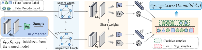
Figure 1: Overall framework of GAPGC for graph test time adaptation. The circle, triangle and square on the left denote three different classes. The green circles represent the selected positive samples with the same pseudo-class as the anchor graph.

Deep neural network models have gained excellent performance under the condition that training and testing data from the same distribution Kipf & Welling (2016); Xu et al. (2018); Zhang et al. (2022a). However, performance suffers when the training data differ from the test data (also called distribution shift) Ding et al. (2021); Li et al. (2022).

Recently test time adaptation has been proposed to improve the performance of OOD test data via model adaptation with test samples and has shown superior performance in the visual domain. For example, Tent Wang et al. (2020) uses entropy minimization as a self-supervised objective during testing, adapting the model by minimizing the entropy of the model predictions on test samples, and TTT Sun et al. (2020) introduces a rotation task as a self-supervised auxiliary task to be jointly optimized with the main task (the target task) during training and to further finetune the trained model during testing, while TTT++ Liu et al. (2021) replaces the rotation task with a contrastive learning task, which can extract discriminative representation by bringing closer the similar instances and separating the dissimilar instances. Despite the encouraging progress, existing TTA schemes are focusing on image data. However, there is still a lack of efficient TTA algorithms tailored for graph data, for which there also exist many OOD circumstances, including molecular property prediction with different molecular scaffolds and protein fold classification with various protein families Ji et al. (2022); Li et al. (2022), etc.

It is imperative to investigate the test time adaptation method tailored for GNNs for the following limitations of the current methods: 1) Unlike images, graph data is irregular and abstract of diverse nature (e.g. citation networks, social networks, and biomedical networks,  Zhang et al. (2022b)), thus image-based methods are not suitable for graphs. For instance, many image augmentation-based methods Ashukha et al. (2020); Zhang et al. (2021) can not be simply extended to graph due to the complication of graph augmentations. 2) Most of data-agnostic approaches involve Entropy Minimization Wang et al. (2020); Niu et al. (2022), which is in effect equivalent to pseudo label Lee et al. (2013). Trusting false pseudo-labels as “ground truth” by encoding them as hard labels could lead to overconfident mistakes (confidence bias) and easily confuse the models Zou et al. (2019). 3) The GNN encoders may learn representations involving the label-irrelevant redundant information through the self-supervised auxiliary task such as contrastive learning Liu et al. (2021), resulting in a sub-optimal performance in the main task Suresh et al. (2021).

To tackle above limitations, we propose Graph Adversarial Pseudo Group Contrast (namely GAPGC), a novel TTA method tailored for GNNs with a contrastive loss variant as the self-supervised objective during testing. Firstly, GAPGC uses group pseudo-positive samples, i.e. a group of graph augmentations with the same class as the anchor graph are selected as the positive samples (Wang et al., 2021a), where the class information comes from the pseudo-labels output by the online test model initialized with the offline trained model. The group pseudo-positive samples enable the contrastive loss to exploit pseudo-labels into model training, bringing useful discriminative information from the well-trained model to the embedding space, thereby enhancing the relevance between the contrastive self-supervised task and the main task. Meanwhile, it also can mitigate the reliance on pseudo-labels and boost the tolerance to incorrect pseudo-labels. This is especially important for label-sensitive graph augmentations.

Secondly, GAPGC adopts adversarial learning to avoid capturing redundant information. Specifically, a Adversarial Learnable Augmenter is proposed to generate aggressive positive samples. On the one hand, GAPGC enforces the augmenter to disturb the original graphs and decrease the information being encoded by maximizing the contrastive loss. On the other hand, GAPGC optimizes the encoder to maximize the correspondence between the disturbed graph pairs by minimizing the contrastive loss. Following such a min-max principle, GAPGC can reduce redundant information for the main task as much as possible, thereby increasing the relevance between the contrastive self-supervised task and the main task. Furthermore we provide theoretical evidence that GAPGC can yield upper bound guarantee of the redundant information from the original graphs from information theory perspective. Empirically, the results on eight different molecular scaffold OOD datasets validate the effectiveness and generalization of our method.

Contributions: 1) We propose a graph test time adaptation method GAPGC tailored for GNNs, based on contrastive learning. The GAPGC explores the trained model knowledge by utilizing pseudo-labels in sample selection, and employs a min-max optimization to pull together the self-supervised task and the main task. To the best of our knowledge, it is the first test time adaptation method tailored for GNNs. 2) The GAPGC alleviates the confidence bias issue caused by entropy minimization (pseudo-labels) through a group of positive samples. Besides, we also provide theoretical evidence that GAPGC can extract minimal sufficient information for the main task from information theory perspective. 3) Experiments on various Scaffold OOD molecular datasets demonstrate that GAPGC achieves state-of-the-art performance for GNN TTA.

2 Related Work

Test Time Adaptation.

Test time adaptation aims to adapt models based on test samples in the presence of distributional shifts. Test time adaptation can be further subdivided into test time training and fully test time adaptation according to whether it can access the source data and alter the training of the source model. Existing test time training methods Sun et al. (2020); Liu et al. (2021) rely on a self-supervised auxiliary task, which is jointly optimized with the main task on the source data and then further finetunes the model on test data. Fully test time adaptation methods with only test data contains batch normalization statistics adaptation Li et al. (2016); Nado et al. (2020); Schneider et al. (2020), prediction entropy minimization Wang et al. (2020); Zhang et al. (2021); Niu et al. (2022), and classifier adjustment Iwasawa & Matsuo (2021). Our work follows the fully test time adaptation setting and aims to design a TTA method tailored for GNNs. We use adversarial contrastive learning with a group pseudo-positive samples to address two key limitations of prior works (i.e.involving redundant information and misleading of incorrect pseudo-labels).

Graph Contrastive Learning.

Recently, contrastive learning (CL) aiming to learn discriminative representation has been widely applied to the visual domain Tian et al. (2020); Chen et al. (2020); Wang et al. (2021a). In GNNs, many GCL methods are arisen for graph representation learning, such as GraphCL You et al. (2020), GRACE Zhu et al. (2020), AD-GCL Suresh et al. (2021) and G-Mixup Han et al. (2022). The performance of GCL heavily relies on the elaborate design of augmentations Zhao et al. (2022). The simple operators like randomly dropping edges or dropping nodes may damage the label-related information and get label-various augmentations Wang et al. (2021b). However, in the self-supervised setting, the dilemma is that model can not directly produce label-invariant augmentations via the current training model  Guo & Sun (2022); Luo et al. (2022). Fortunately, GAPGC uses the decent trained model to generate the relatively reliable pseudo-labels, avoiding the severe model shift caused by the incorrect positive samples.

Table 1: Test ROC-AUC (%) of GIN(contexpred) on molecular property prediction benchmarks with OOD split.(’$\uparrow$’ denotes performance improvement compared to the pure test baseline. PF: parameter-free.)

Methods	BBBP	Tox21	Toxcast	SIDER	ClinTox	MUV	HIV	BACE	Average
# Test Molecules	203	783	857	142	147	9308	4112	151	$\diagup$
# Binary prediction task	1	12	617	27	2	17	1	1	$\diagup$
Test (baseline)	69.23	75.44	63.68	59.70	68.94	78.32	77.52	80.16	71.62
Tent Wang et al. (2020)	68.80	74.70	63.41	59.50	69.68	78.18	76.72	80.39	71.42
BN Ada. Schneider et al. (2020)	69.31	75.30	63.95	60.09	71.59	78.63	77.34	80.26	72.06
SHOT Liang et al. (2020)	69.46	74.84	63.77	60.47	68.52	79.05	77.57	80.19	71.73
PF-GAPGC (ours)	69.25	75.33	63.89	59.93	72.92	78.91	78.14	82.80	72.65
GAPGC (ours)	70.34$\uparrow_{1.11}$	76.00$\uparrow_{0.56}$	64.58$\uparrow_{0.90}$	60.85$\uparrow_{1.15}$	72.92$\uparrow_{3.98}$	80.17$\uparrow_{1.85}$	78.63$\uparrow_{1.11}$	83.03$\uparrow_{2.87}$	73.31$\uparrow_{1.69}$

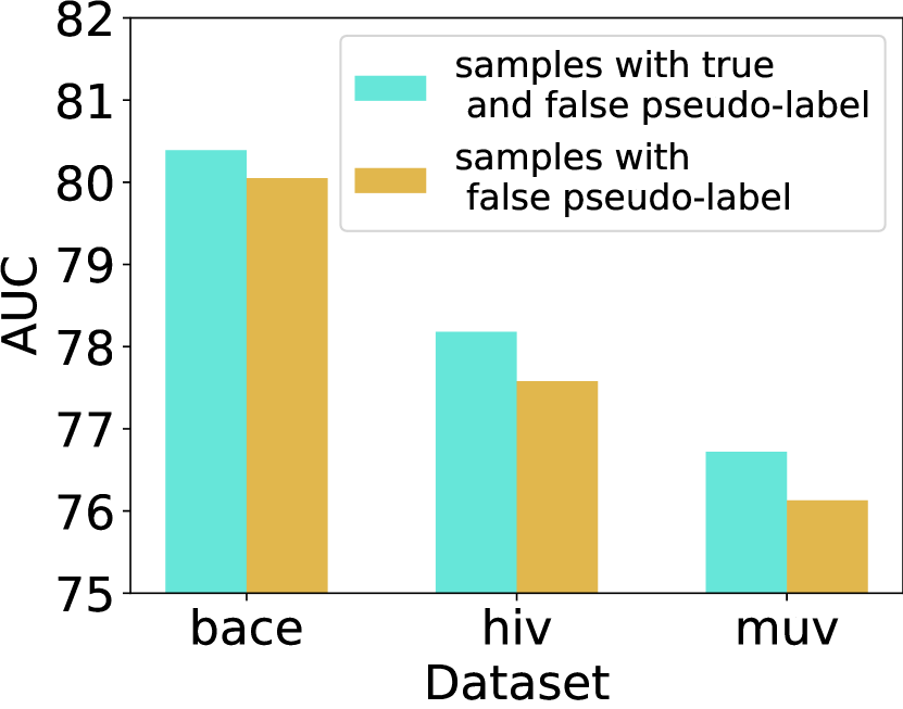
(a)

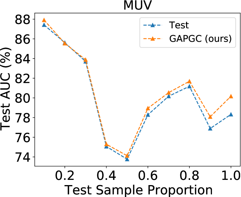
(b)

Figure 2: (a) Entropy minimization performed on test samples with only false pseudo-label will degrade the performance, compared with that performed on all test samples with both true pseudo-label and false pseudo-label. (b) AUC with different proportion of test data during testing.

3 Graph Adversarial Pseudo Group Contrast

Notations.

We use boldface letter $\mathbf{x}\in\mathbb{R}^{n}$ to denote an $n$-dimensional vector, where $\mathbf{x}(i)$ is the $i^{\text{th}}$ entry of $\mathbf{x}$. Let $G=(V,E)$ be a graph with vertices $V$ and edges $E$. We denote by $\mathbf{A}\in\mathbb{R}^{|\mathcal{V}|\times|\mathcal{V}|}$ the adjacency matrix of $G$. Suppose $G$ has node features $\{\mathbf{x}_{i}\in\mathbb{R}^{F}\}_{i=1}^{|V|}$. For test time adaptation, we denote the previously trained model as $f_{\Phi}$, in which $\Phi$ consists of the learnable parameters of encoder $\Phi_{1}$ and classifier $\Phi_{2}$ respectively.

To address those challenges mentioned in the introduction and better adapt the trained model to test dataset online, we propose a new graph test time adaptation method based on a novel Adversarial Pseudo Group Contrast strategy.

3.1 Group Pseudo-Positive Samples for Graph CL

Here, we aim at adapting the model via utilizing the informative pseudo-labels (i.e. the output of the model) during test time. However, as alluded to earlier in the introduction, directly using the entropy minimization would push the probability of a false pseudo-label sample as sharp as possible, thus causing the overconfidence mistake and confusing the model during TTA (c.f. Fig. 2(a)). To avoid this problem, we use a Contrastive Learning variant to better explore the pseudo-labels. In the CL variant, a number of the same pseudo-class augmentations are selected to mitigate the reliance on pseudo-labels and enhance the tolerance to false labels. Specially, for each anchor graph $G_{i}$ in test set, its representation $\mathbf{z}_{i}=h(f_{\Phi_{1}}(G_{i}))$ as well as its augmentation $\mathbf{z}_{i}^{a}=h(f_{\Phi_{1}}(G_{i}^{a}))$ are generated by the GNN encoder $f_{\Phi_{1}}$ following with a projection head $h$ ($2$-layer MLP), where $G_{i}^{a}$ is an augmentation of $G_{i}$ sampling from a given Graph Data Augmentation (GDA) $T(G_{i})$. Then we obtain the pseudo-label of $G_{i}$ by forwarding the classifier $f_{\Phi_{2}}$, i.e. $\hat{y}_{i}=\text{arg}\max_{c}{f_{\Phi_{2}}(f_{\Phi_{1}}(G_{i})}))$.

Instead of using only one positive sample in standard contrastive loss, a group of positive samples $\mathcal{S}^{p}=\{\mathbf{z}_{d}^{a,\hat{y}_{i}}\}_{d=1}^{D}$ in a mini-batch (suppose the size is $m>D$) are chosen according to the anchor pseudo-label $\hat{y}_{i}$. In addition, all augmentations with other class $\{\mathbf{z}_{i}^{a,\hat{y}}:\hat{y}\in\{1,2,\cdots,C\}\setminus\hat{y_{i}}\}$ are acted as negative samples. Finally, the contrastive loss variant can be formulated as follows:

$$\hat{\mathcal{L}} (f_{\Phi},\{(G_{i})\}_{i=1}^{m},\{G_{i}^{a}\}_{i=1}^{m})$$

$$:=\frac{-1}{m}\sum_{i=1}^{m}\mathcal{F}(\{\log\frac{\exp(s(\mathbf{z}_{i},\mathbf{z}_{d}^{a,\hat{y}_{i}}))}{\sum_{j=1}^{m}\exp(s(\mathbf{z}_{i},\mathbf{z}_{j}^{a}))}\}_{d=1}^{D}),$$ (1)

where $\sum_{j=1}^{m}\exp(s(\mathbf{z}_{i},\mathbf{z}_{j}^{a}))$ represents the sum of every pairs of anchor $\mathbf{z}_{i}$ in a min-batch, $s$ is the cosine similarity, and $\mathcal{F}:\mathbb{R}^{D}\to\mathbb{R}$ denotes a general multivariate function, such as the mean function. If not specifically stated, we default to $\mathcal{F}$ as the mean function throughout this paper. It is conspicuous that the loss $\hat{\mathcal{L}}$ maximizes the similarity between the anchor graph $G$ and its positive samples $\mathcal{S}^{p}$. When some pseudo-labels in $\mathcal{S}^{p}$ are error, those samples with true pseudo-labels will win this instance conflict since their representations are more similar to the anchor compared with the false ones. The group pseudo-positive samples take advantage of pseudo-labels and enhance the tolerance to false labels, effectively alleviating the confidence bias. It’s worth noting that the group positive samples are particularly suitable for graph CL since graph augmentations are always label-sensitive. For example, in a molecular graph dataset, supposing that all molecular graphs containing a cycle are labeled as toxic. If we drop any node belonging to the cycle, it will damage this cyclic structure, mapping a toxic molecule to a non-toxic one.

3.2 Adversarial Learnable Augmenter for Graph CL

On test time adaptation, the self-supervised task should only concentrate on the performance of the main task. TTT++Liu et al. (2021) can enhance the relevant between the contrastive learning auxiliary task with the main task by jointly optimizing on source data. However, in our setting without access to source data, directly optimizing the contrastive loss $\hat{\mathcal{L}}$ is insufficient to obtain a promising performance for the main task (c.f. Table 2) since the contrastive learning would capture the redundant information that is irrelevant to downstream tasks. This phenomenon has been well studied in early literature under the representation learning context Tschannen et al. (2019); Suresh et al. (2021). In order to reduce the redundant information, we adopt the adversarial learning strategy upon the contrastive learning framework. A trainable GNN-based augmenter optimized by maximizing the contrastive loss is used to decrease the amount of information being encoded.

Learnable Augmenter.

Here we use a learnable edge-dropping augmentation. For a graph $G$, $T(G)$ is an augmentation of $G$ obtained by dropping some edges from $G$. This can be done by setting the edge weights $e_{ij}$ of $T(G)$ as a binary variable, where edge $(i,j)$ is selected if $e_{ij}=1$ and is dropped otherwise. The binary variable can be regarded as following a Bernoulli distribution with a parameter denoted as $w_{ij}$, where $P(e_{ij}=1)=w_{ij}$. We parameterize the Bernoulli parameter $w_{ij}$ with a GNN-based augmenter initialized from the offline trained model. Further, to make the augmenter trainable, we relax the edge weights to continue variable in (0,1) with the reparameterization trick Maddison et al. (2016). Specifically, the weight $\hat{e}_{ij}$ of edge $(i,j)$ is calculated by:

$$\omega_{ij}=\text{MLP}([\mathbf{h}_{i},\mathbf{h}_{j}]),\quad\delta\backsim\text{Uniform}(0,1)$$ (2)

$$\hat{e}_{ij} =\text{Sigmoid}((\log\delta-\log(1-\delta)+\omega_{ij})/\tau)$$ (3)

where $\mathbf{h}_{i}$ is the $i$-th node representation output by GNN encoder $g_{\Theta_{1}}(G)$, and $\Theta$ corresponds to the learnable parameters of GNN encoder ($\Theta_{1}$) as well as MLP ($\Theta_{2}$). Note that $e_{ij}$ is approximated to binary when the temperature hyper-parameter $\tau\to 0$. Besides, the regularization term $\mathcal{L}_{e}=\sum_{ij}\omega_{ij}/|E|$ is also added to prevent the excessive perturbation.

Min-Max Game.

The GAPGC TTA framework is constructed following a min-max principle:

$$\max\limits_{\Theta}\min\limits_{\Phi}{\mathcal{L}}_{GAPGC}(f_{\Phi},g_{\Theta},\{G_{i}\}_{i=1}^{m})=$$

$$\max\limits_{\Theta}\min\limits_{\Phi}(\hat{\mathcal{L}}(f_{\Phi},\{G_{i}\}_{i=1}^{m},\{g_{\Theta}(G_{i})\}_{i=1}^{m})+\lambda\mathcal{L}_{e})$$ (4)

where $\lambda$ is the regularization weight. This objective contains two folds: (1) Optimize encoder $f_{\Phi_{1}}$ to pull an anchor and a number of pseudo-positive samples together in the embedding space, while pushing the anchor away from many negative samples; (2) Optimize the the augmenter $g_{\Theta}$ to maximize such a contrastive loss. Overall, the min-max optimization expects to train an encoder that is capable of maximizing the similarity between the original graph and a set of augmentations even though the augmentations are very aggressive (i.e. the $T(G)$ is clearly different with $G$).

The interpretation from information bottleneck perspective shows that the objective can provide a lower bound guarantee of the information related to the main task, while simultaneously holding a upper bound guarantee of the redundant information from the original graphs, with the details can be seen in Appendix B due to the space limitation. Finally, this objective can get representations containing minimal information that is sufficient to identify each graph.

Discussion.

a) A recent approach called PGC (Pseudo Group Contrast ) Wang et al. (2021b) shares a similar manner with our group pseudo-positive samples for GCL. However, they are different in the following aspects: (1) GAPGC aims at working for TTA (self-supervised) while PGC is designed for self-tuning (self-training + fine-tuning), and the former explores the test data without any labels while the latter needs both labeled and unlabeled data. (2) GAPGC uses adversarial learning to generate the hard positive samples and reduce the redundant information between input graphs and graph representations while PGC is only designed for image data with simple augmentations. b) The style of learnable edge-dropping augmentation has also been used in representation learning AD-GCL Suresh et al. (2021). The difference between our method with AD-GCL is that (1) we parameterize the Bernoulli weights with a GNN-based augmenter initialized from the offline trained model, while AD-GCL uses another GNN trained from scratch, and (2) our augmenter is optimized by a contrastive loss variant with group pseudo-positive samples, different from AD-GCL.

Table 2: The results of ablation study on GAPGC(ROC-AUC %). ALA means Adversarial Learnable Augmenter and GPPS represents Group Pseudo-Positive Samples.

Methods	BBBP	Tox21	Toxcast	SIDER	ClinTox	MUV	HIV	BACE	Average
test (baseline)	69.23	75.44	63.68	59.70)	68.94	78.32	77.52	80.16	71.62
w/ Both	69.98	75.72	64.18	60.21	71.79	80.17	78.32	82.28	72.83
w/o ALA	68.90	75.39	64.42	59.85	70.98	82.50	77.67	81.05	72.60
w/o GPPS	69.94	75.40	64.41	59.70	71.25	76.94	77.31	81.97	72.12
w/o Both	68.87	75.38	64.47	59.78	70.91	80.09	77.57	80.93	72.25

4 Experiment

We conduct experiments on molecular scaffold OOD datasets to evaluate our method. The multi-task style version is deferred to the appendix due to the space limitation.

4.1 Molecular Property Prediction

Settings.

We use the same model architecture and datasets in Hu et al. (2019). Dataset: eight binary classification datasets in MoleculeNet Wu et al. (2018) is used and the data split follows the OOD split principle: scaffold split. The split ratio for the train/validation/test sets is $8$:$1$:$1$. Architecture: A 5-layer GIN Xu et al. (2018). We first directly initialize the model with a pretrained model GIN (contextpred) released at (https://github.com/snap-stanford/pretrain-gnns), which is pretrained via the Context Prediction on Chemistry dataset. Then the model would be trained on the training set offline and finally adapted on the testing set online to evaluate TTA methods. More details of the experimental settings can be referred to the appendix .

Baselines.

Since we have not found related works about test time adaptation on graph data, we extend several state-of-the-art baselines designed for Convolutional Neural Networks to GNNs: Tent, BN Adaptation, and SHOT. Specifically, Tent (Wang et al., 2020) minimizes the entropy of the model predictions on test data during testing. BN Schneider et al. (2020) updates the batch normalization statistics according to the test samples. SHOT Liang et al. (2020) exploits both information maximization and self-supervised pseudo-labeling during testing.

PF-GAPGC: Parameter-Free GAPGC.

In test time training, since it is not able to access the training data, the projection head $h$ and MLP $g_{\Theta_{2}}$ can not get an ideal weights initialization when the number of test data points is extremely small. To address this problem, we extend GAPGC to a parameter-free version, i.e. using only the weights of the trained model and not introducing any extra learnable parameters. i) Remove Projection Head. Although many works have shown that the projection head is vital for improving the expressive power of representations  Chen et al. (2020); Luo et al. (2022), it will be better to remove it when we don’t have enough data to train Chen et al. (2022). ii) Parameter-Free $g_{\Theta_{2}}$. We directly replace MLP $g_{\Theta_{2}}$ in Eq. (2) with a inner product for removing the extra parameters $\Theta_{2}$, i.e.

$$\omega_{ij}=\frac{\mathbf{h}_{i}^{\top}\mathbf{h}_{j}}{\|\mathbf{h}_{i}\|_{2}\|\mathbf{h}_{j}\|_{2}}$$ (5)

where $\|\cdot\|$ is $L_{2}$ norm. Note that after this replacement, $g_{\Theta}$ can be seen as a graph inner product decoder variant.

Results.

The results compared with different TTA methods are shown in Table 1. Obs. (1): Both PF-GAPGC and GAPGC improve over all the baselines on average, and GAPGC consistently gains the best performance among all the baselines in all different datasets, suggesting its generalization and robustness. And since GAPGC is better than PF-GAPGC, it demonstrates that the contrastive projector $h$ and MLP in augmenter $g_{\Theta}$ can learn well even though they have not been pre-trained offline. Obs. (2): The performance of Tent is worse than the test baseline on average, indicating that directly using entropy minimization may lead to negative transfer. This may be caused by optimizing the entropy is biased to predict only a particular class, which will hurt the performance in the binary classification problem, as illustrated in Fig. 2(a). Besides, SHOT only gives a small performance improvement, further implying the limitations of entropy minimization for this binary classification task on graphs.

4.2 Ablation Study

1) Effects of Different Components.

We conduct ablation experiments to verify the efficiency of the proposed two components: Adversarial Learnable Augmenter (ALA) and Group Pseudo-Positive Samples (GPPS). The results are shown in Table 2, where without Adversarial Learnable Augmenter means randomly edge-dropping augmentation is used instead, while without Group Pseudo-Positive Samples represents only the correspondent augmentation of the anchor graph is used as its positive sample in the contrastive loss. Obs. (1): The four models all outperform the test baseline, verifying that contrastive learning as a self-supervised task during testing can improve test performance. Obs. (2): The variant ’w/o ALA’ is better than the variant ’w/o GPPS’, demonstrating that the Adversarial Learnable Augmenter contributes more in GAPGC. Obs. (3): The combination of these two components achieves the best performance on average.

2) Effects of Different Proportion of Test Samples.

In actual deployment, test data may come in batches of different sizes. Here we evaluate the effectiveness of GAPGC under different proportions of test data. As described in Fig. 2(b), our GAPGC can consistently gain performance improvement compared with the pure test baseline under different proportions of test data.

5 Conclusions and Limitations

We propose a graph test time adaptation strategy GAPGC for the graph OOD problem. Despite the good results, there are some aspects worth exploring further in the future: i) The parameterized augmenter can generalize to other learnable graph generators. ii) The GCL projector and augmenter’s MLP can be initialized offline by training on public datasets (e.g., Chemistry dataset) prior to deployment.

Appendix

.tocmtappendix mtchapternone mtappendixsubsection

Appendix A GAPGC for Multi-tasks

A.1 Multi-Tasks

Multi-labels Similarity.

We define a similarity between two multi-labels for selecting the positive samples in a min-batch.

Definition A.1.

Given the label of two n-task samples $y_{1}=(t_{1},t_{2},\cdots,t_{n})$, $y_{2}=(l_{1},l_{2},\cdots,l_{n})$, where $t_{i}\in\{0,1\}$and $l_{i}\in\{0,1\}$ for all $i\in\{1,2,\cdots,n\}$. The similarity between $y_{1}$ and $y_{2}$ can be defined as

$$sim(y_{1},y_{2})=\frac{1}{n}\sum_{i=1}^{n}\mathbf{1}(t_{i}=l_{i})$$ (6)

Positive Sample Selection.

In GAPGC, suppose that we get the pseudo-label of anchor is $\hat{y}=[y_{1},y_{2},\cdots,y_{n}]$ and its augmentation pseudo-label is $\hat{y}^{a}=[y_{1}^{a},y_{2}^{a},\cdots,y_{n}^{a}]$. The similarity can be calculated by the $sim(\hat{y},\hat{y}^{a})$.

Since $sim\in[0,1]$ is a real number, we use a threshold $\gamma\in[0,1]$ to decide whether the the augmentation graph can be selected as positive sample, i.e.

$$\mathcal{Y}(\hat{y},\hat{y}^{a})=\begin{cases}0,&\text{if }sim(\hat{y},\hat{y}^{a})<\gamma\\ 1,&\text{if }sim(\hat{y},\hat{y}^{a})\geq\gamma\end{cases}$$ (7)

$\mathcal{Y}(\hat{y},\hat{y}^{a})=1$ represents the augmentation is selected otherwise is not selected.

Appendix B Theoretical Analysis From Graph Information Bottleneck

In this part, we show the GAPGC is actually very closely linked to the GIB Wu et al. (2020), which minimizes the mutual information between input graph and graph representation and simultaneously maximizes the mutual information between representation and output, i.e.$\min_{f}[I(f(G);G)-\beta I(f(G);Y)]$.

Different from the existing works AD-GCL Suresh et al. (2021) that just provides the connection between standard adversarial contrastive loss and GIB, here we give a more general version based on GAPGC.

Min-Max Mutual Information.

We consider $\mathcal{F}$ as a general multivariate function to investigate a comprehensive conclusion about the GAPGC and mutual information. The results show below.

Proposition 1.

Let $\mathbf{z}_{i}=h(f_{\Phi_{1}}(G_{i}))$ and $\mathbf{z}_{d}^{a,\hat{y}_{i}}=h(f_{\Phi_{1}}(G_{d}^{a,\hat{y}_{i}}))$ denote the representation of anchor graph $G_{i}$ and a positive augmentation $G_{d}^{a,\hat{y}_{i}}$, respectively. where $\hat{y}_{i}={arg}\max_{c}{f_{\Phi_{2}}(f_{\Phi_{1}}(g_{\Theta}(G_{i})}))$ is the pseudo-label of $G_{i}$. If $\mathcal{F}$ is a multivariate function satisfying

i) enables exchange order with expectation, and

ii) monotonically non-decreases for each component,

then the contrastive loss in Eq. (1) can be bounded by

$$\mathcal{F}(\{I(\mathbf{z}_{i},\mathbf{z}_{d}^{a,\hat{y}_{i}})\}_{d=1}^{D})\geq\mathcal{F}(\log(m))-\hat{\mathcal{L}}_{GAPGC}$$ (8)

where $g_{\theta}(G)$ is the parameterized augmenter, composed of a GNN encoder $g_{\Theta_{0}}$ and a MLP decoder $g_{\Theta_{1}}$.

Therefore, the Eq. (4) is approximately equivalent to optimizing the transformation ($\mathcal{F}$ is the transform function) of mutual information between the anchor graph and its positive samples. Formally, we have

$${\mathcal{L}}_{GAPGC}\thickapprox\min\limits_{\Theta}\max\limits_{\Phi}\mathcal{F}\left(\{I(f_{\Phi}(G_{i});f_{\Phi}(g_{\Theta}(G_{d}^{a,\hat{y}_{i}})))\}_{d=1}^{D}\right)$$ (9)

Note that the mean function is a multivariate function that satisfies the conditions in Proposition 1. For clarity, we rewrite $g_{\Theta}$ as a graph data augmentation family $\mathcal{T}$ and omit the subscript $\Theta$ of $f_{\Theta}$. We have

$${\mathcal{L}}_{GAPGC}\thickapprox\min\limits_{T\in\mathcal{T}}\max\limits_{f}\mathcal{F}\left(\{I(f(G);f(t(G_{d}^{a,\hat{y}_{i}})))\}_{d=1}^{D}\right),\text{where }t(G)\backsim T(G)$$ (10)

Graph Information Bottleneck (GIB).

We theoretically describe the property of the encoder online trained via GAPGC and explain it by GIB.

Proposition 2.

Assume that the GNN encoder $f$ has the same power as the 1-WL test and $\mathcal{F}$ satisfies the conditions in proposition  1. Suppose $\mathcal{G}$ is a countable space and thus quotient space $\mathcal{G}^{\prime}=G/\cong$ is a countable space, where $\cong$ denotes equivalence ($G_{1}\cong G_{2}$ if $G_{1},G_{2}$ cannot be distinguished by the 1-WL test). Define $\mathbb{P}_{\mathcal{G}^{\prime}\times\mathcal{Y}}(G^{\prime},Y^{\prime})=\mathbb{P}_{\mathcal{G}\times\mathcal{Y}}(G\cong G^{\prime},Y)$ and $T^{\prime}(G^{\prime})=\mathbb{E}_{G\backsim\mathbb{P}_{\mathcal{G}}}[T^{*}(G)|G\cong G^{\prime}]$ for $G^{\prime}\in\mathcal{G}$. Then, the optimal solution $(f^{*},T^{*})$ to GAPGC satisfies

1. $\mathcal{F}\left(\{I(f^{*}(t^{*}(G_{d}));G|Y)\}_{d=1}^{D}\right)\leq\min_{T\in\mathcal{T}}\mathcal{F}(\{I(t^{\prime}(G^{\prime}_{d});G^{\prime})-I(t^{\prime*}(G^{\prime}_{d});Y)\}_{d=1}^{D})$, where $t^{*}(G_{d})\backsim T^{*}(G),t^{\prime}(G_{d}^{\prime})\backsim T^{\prime}(G^{\prime}),t^{\prime*}(G_{d}^{\prime})\backsim T^{\prime*}(G^{\prime}),(G,Y)\backsim\mathbb{P}_{\mathcal{G}\times\mathcal{Y}}$.

2. $\mathcal{F}\left(\{I(f^{*}(G);Y)\}_{d=1}^{D}\right)\geq\mathcal{F}\left(\{I(f^{*}(t^{\prime*}(G^{\prime}_{d}));Y)\}_{d=1}^{D}\right)=\mathcal{F}\left(\{I(t^{\prime*}(G_{d}^{\prime});Y)\}_{d=1}^{D}\right)$, where $t^{\prime*}(G_{d}^{\prime})\backsim T^{\prime*}(G^{\prime}),(G,Y)\backsim\mathbb{P}_{\mathcal{G}\times\mathcal{Y}}$ and $(G^{\prime},Y)\backsim\mathbb{P}_{\mathcal{G}^{\prime}\times\mathcal{Y}}$.

The left side of inequality in statement 1 measures the redundant information that is embedded in representations but irrelevant to the main tasks during TTA. i) The result in statement 1 of proposition 2 suggests that the redundant information have a GIB style upper bound, since $\min_{T\in\mathcal{T}}I(t^{\prime}(G^{\prime});G^{\prime})-I(t^{\prime*}(G^{\prime});Y)\geq\min_{f}[I(f(G);G)-I(f(G);Y)]$ (i.e. $\beta=1$ of GIB). Therefore, the encoder trained by GAPGC enables encoding a representation that only has limited redundant information.

ii) The statement 2 shown that $\mathcal{F}\left(\{I(t^{\prime*}(G_{d}^{\prime});Y)\}_{d=1}^{D}\right)$ can act as a lower bound of the mutual information between the learnt representations and the labels of the main tasks. Therefore, optimizing the GDA family $\mathcal{T}$ allows $\mathcal{F}\left(\{I(f^{*}(t^{*}(G_{d}));Y)\}_{d=1}^{D}\right)$ to achieve a larger value. This implies that it is better to regularize when learning over $\mathcal{T}$ . In the GAPGC loss, based on edge-dropping augmentation, we follow  Suresh et al. (2021) to regularize the ratio of dropped edges per graph.

When $\mathcal{F}$ is a mean function, the statement 2 can be rewritten as:

$$I(t^{\prime*}(G_{d}^{\prime});Y)\geq\frac{1}{D}\sum_{d=1}^{D}I(f^{*}(t^{\prime*}(G^{\prime}_{d}));Y)$$ (11)

Appendix C Missing Proof.

See 1

Proof.

From Oord et al. (2018), we easily get a lower bound of mutual information between $z_{i}$ and $z_{j}^{a}$.

$$\mathbb{E}_{(G,G^{\hat{y},d})}\left[\log\frac{\exp(s(\mathbf{z}_{i},\mathbf{z}_{d}^{a,\hat{y}_{i}})}{\sum_{j=1}^{m}\exp(s(\mathbf{z}_{i},\mathbf{z}_{j}^{a}))}\right] =\frac{1}{m}\sum_{i=1}^{m}\log\frac{\exp(s(\mathbf{z}_{i},\mathbf{z}_{d}^{a,\hat{y}_{i}})}{\sum_{j=1}^{m}\exp(s(\mathbf{z}_{i},\mathbf{z}_{j}^{a}))}$$ (12)

$$\leq I(\mathbf{z}_{i},\mathbf{z}_{d}^{a,\hat{y}_{i}})-\log(m)$$ (13)

$$\hat{\mathcal{L}}_{GAPGC}:=-\mathbb{E}_{(G,G^{\hat{y}})}\left[\mathcal{F}(\{\log\frac{\exp(s(\mathbf{z}_{i},\mathbf{z}_{d}^{a,\hat{y}_{i}})}{\sum_{j=1}^{m}\exp(s(\mathbf{z}_{i},\mathbf{z}_{j}^{a}))}\}_{d=1}^{D})\right]=-\frac{1}{m}\sum_{i=1}^{m}\mathcal{F}(\{\log\frac{\exp(s(\mathbf{z}_{i},\mathbf{z}_{d}^{a,\hat{y}_{i}})}{\sum_{j=1}^{m}\exp(s(\mathbf{z}_{i},\mathbf{z}_{j}^{a}))}\}_{d=1}^{D})$$ (14)

where $\mathcal{F}:\mathbb{R}^{d}\to\mathbb{R}$ is a general multivariate function, which can be designed a learnable neural network such as MLP, Attention networks.

Since $\mathcal{F}$ can exchange order with expectation, then we have

$$\mathbb{E}_{(G,G^{\hat{y}})}\left[\mathcal{F}(\{\log\frac{\exp(s(\mathbf{z}_{i},\mathbf{z}_{d}^{a,\hat{y}_{i}})}{\sum_{j=1}^{m}\exp(s(\mathbf{z}_{i},\mathbf{z}_{j}^{a}))}\}_{d=1}^{D})\right] =\mathcal{F}(\{\mathbb{E}_{(G_{i},G_{i}^{\hat{y}})}\left[\log\frac{\exp(s(\mathbf{z}_{i},\mathbf{z}_{d}^{a,\hat{y}_{i}})}{\sum_{j=1}^{m}\exp(s(\mathbf{z}_{i},\mathbf{z}_{j}^{a}))}\right]\}_{d=1}^{D})$$ (15)

$$\leq\mathcal{F}(\{I(z_{i},\mathbf{z}_{d}^{a,\hat{y}_{i}})-\log(m)\}_{d=1}^{D})$$ (16)

If $\mathcal{F}$ is monotonically non-decreasing for each component, minimizing $\hat{\mathcal{L}}_{GAPGC}$ is equivalent to maximize the lower bound of $\mathcal{F}\left(\{I(f_{\Phi_{1}}(G);f_{\Phi_{1}}(g_{\Theta}(G_{d}^{\hat{y}})))\}_{d=1}^{D}\right)$.

In our experiments, we use the mean function as an instance.

∎

See 2

Proof.

Our proof based on the lemma below.

Lemma C.1 (Suresh et al. (2021), theorem 1).

Suppose the encoder $f$ is implemented by a GNN as powerful as the 1-WL test. Suppose $\mathcal{G}$ is a countable space and thus $\mathcal{G}^{\prime}$ is a countable space. Then, the optimal solution $(f^{*},T^{*})$ to $\min_{T\in\mathcal{T}}\max_{f}I(f(G),f(t(G)))$ satisfies, letting $T^{\prime*}(G^{\prime})=\mathbb{E}_{G\backsim\mathbb{P}_{G}}[T^{*}(G)|G\cong G^{\prime}]$,

1.

$$I(f^{*}(t^{*}(G));G|Y)\leq\min_{T\in\mathcal{T}}I(t^{\prime}(G^{\prime});G^{\prime}))-I(t^{\prime*}(G^{\prime});Y),$$ (17)

where $t^{*}(G)\backsim T^{*}(G),t^{\prime}(G^{\prime})\backsim T^{\prime}(G^{\prime}),t^{\prime*}(G^{\prime})\backsim T^{\prime*}(G^{\prime}),(G,Y)\backsim\mathbb{P}_{\mathcal{G}\times\mathcal{Y}}$ and $(G^{\prime},Y)\backsim\mathbb{P}_{\mathcal{G}^{\prime}\times\mathcal{Y}}.$

2. $I(f^{*}(G);Y)\geq I(f^{*}(t^{\prime*}(G^{\prime}));Y)=I(t^{\prime*}(G^{\prime});Y)$, where $t^{*}(G)\backsim T^{*}(G),t^{\prime*}(G^{\prime})\backsim T^{\prime*}(G^{\prime}),(G,Y)\backsim\mathbb{P}_{\mathcal{G}\times\mathcal{Y}}$ and $(G^{\prime},Y)\backsim\mathbb{P}_{\mathcal{G}^{\prime}\times\mathcal{Y}}$.

In lemma C.1, we know for each anchor-augmentation pair, the mutual information between them can be bounded by $I(f^{*}(t^{*}(G_{d}));G|Y)\leq\min_{T\in\mathcal{T}}I(t^{\prime}(G_{d}^{\prime});G^{\prime}))-I(t^{\prime*}(G_{d}^{\prime});Y),d=1,2,\cdots D$. So we use the $\mathcal{F}$ to act on two sides of Eq. (17), then we get

$$\mathcal{F}(\{I(f^{*}(t^{*}(G_{d}));G|Y)\}_{d=1}^{D})\leq\mathcal{F}(\{\min_{T\in\mathcal{T}}I(t^{\prime}(G_{d}^{\prime});G^{\prime}))-I(t^{\prime*}(G_{d}^{\prime});Y)\}_{d=1}^{D}),$$ (18)

Since the $\mathcal{F}$ is monotonically non-decreases for each component, we have $\mathcal{F}(\{\min_{T\in\mathcal{T}}I(t^{\prime}(G_{d}^{\prime});G^{\prime}))-I(t^{\prime*}(G_{d}^{\prime});Y)\}_{d=1}^{D})\leq\min_{T\in\mathcal{T}}(\mathcal{F}(\{I(t^{\prime}(G_{d}^{\prime});G^{\prime}))-I(t^{\prime*}(G_{d}^{\prime});Y)\}_{d=1}^{D})$. Thus,

$$\mathcal{F}(\{I(f^{*}(t^{*}(G_{d}));G|Y)\}_{d=1}^{D})\leq\min_{T\in\mathcal{T}}(\mathcal{F}(\{I(t^{\prime}(G_{d}^{\prime});G^{\prime}))-I(t^{\prime*}(G_{d}^{\prime});Y)\}_{d=1}^{D})$$ (19)

Similarly, the statement 2 can be obtained due to the monotonicity of $\mathcal{F}$

$$\mathcal{F}(\{I(f^{*}(G);Y)\}_{d=1}^{D})\geq\mathcal{F}\left(\{I(f^{*}(t^{\prime*}(G^{\prime}_{d}));Y)\}_{d=1}^{D}\right)=\mathcal{F}\left(\{I(t^{\prime*}(G_{d}^{\prime});Y)\}_{d=1}^{D}\right)$$ (20)

∎

Appendix D Details of Experiments.

Settings.

In our experiments, we fix the weights of classifier $f_{\Phi_{2}}$ for alleviating the over-fitting and Catastrophic Forgetting in TTA Niu et al. (2022) and improving the model generalization.

Baselines: Tent (Wang et al., 2020) minimizes the entropy of model prediction during testing. BN Schneider et al. (2020) updates the batch normalization statistics according to the test samples. SHOT Liang et al. (2020) exploits both information maximization and self supervised pseudo-labeling to implicitly align representations from the target domains to the source hypothesis.

Datasets: The eight molecular datasets used are summarized in Table 3.

Table 3: Statistical information of the datasets. We provide (median, max, min, mean, std) number of graph vertices in different datasets.

dataset	# Molecules	# training set	median	max	min	mean	std
BBBP	2039	1631	22	63	2	22.5	8.1
Tox21	7831	6264	14	114	1	16.5	9.5
Toxcast	8575	6860	14	103	2	16.7	9.7
SIDER	1427	1141	23	483	1	30.0	39.7
ClinTox	1478	1181	23	121	1	25.5	15.3
MUV	93087	74469	24	44	6	24.0	5.0
HIV	41127	32901	23	222	2	25.3	12.0
BACE	1513	1210	32	66	10	33.6	7.8

Datasets Splitting: We follow the Out Of Distribution data split principle in Hu et al. (2019): scaffold split, in which, molecules are clustered by scaffold (molecular graph substructure), and then the dataset is split so that different clusters end up in the training, validation and test sets.

Hyper-parameter Strategy: We use Adam optimizer with $L_{2}$ regularization during test time. For all hyper-parameters, we use grid search strategies and the range of hyper-parameters listed in Table 4, 5, where Table 4 shows our methods and Table 5 shows the baselines.

Table 4: Hyper-parameter search range for GAPGC.

Hyper-parameter	Range
$\lambda$	{0.1, 1, 10, 20, 50}
$\gamma$	{0.6, 0.7, 0.8, 0.9, 1.0}
Learning rate	{0.001, 0.005, 0.01,0.0005,0.0001}
Weight decay	{1e-2, 1e-3,1e-4,5e-4, 1e-5,1e-6,1e-7,0}
Dropout rate	{0,0.05,0.1,0.15,0.2,0.25,0.3,0.35, 0.4,0.45, 0.5}
Batch size	{32,64,128,256,512}
Optimizer	Adam
TTA Epoch	1
runseed	1
GPU	Tesla V100

Table 5: Hyper-parameter search range for Baselines.

Hyper-parameter for Tent	Range
Learning rate	{0.001, 0.005, 0.01,0.0005,0.0001}
Weight decay	{1e-2, 1e-3,1e-4,5e-4, 1e-5,1e-6,1e-7,0}
Batch size	{32,64,128,256,512}
Optimizer	Adam
Hyper-parameter for BN	Range
Batch size	{32,64,128,256,512}
Hyper-parameter for SHOT	Range
Learning rate	{0.001, 0.005, 0.01,0.0005,0.0001}
Weight decay	{1e-2, 1e-3,1e-4,5e-4, 1e-5,1e-6,1e-7,0}
$\beta$	{0 0.1, 0.2, 0.3,0.4,0.5,0.7,0.8,0. 1}
Batch size	{32,64,128,256,512}
Optimizer	Adam

Appendix E Additional Experiments.

We conduct experiments on molecular scaffold OOD datasets with the non pre-trained GIN model, that is, directly training GIN on the training set of OOD datasets without weights initialization from the pretrained model provided by Hu et al. (2019). The results show in Table 6.

Table 6: Test ROC-AUC (%) of GIN on molecular property prediction benchmarks with OOD split.(’$\uparrow$’ denotes performance improvement compared to the pure test baseline. PF: parameter-free.)

Methods	BBBP	Tox21	Toxcast	SIDER	ClinTox	MUV	HIV	BACE	Average
# Test Molecules	203	783	857	142	147	9308	4112	151	$\diagup$
# Binary prediction task	1	12	617	27	2	17	1	1	$\diagup$
Test (baseline)	64.56	72.57	63.72	57.81	65.54	71.06	72.85	74.54	67.83
Tent Wang et al. (2020)	65.17	72.46	63.83	60.35	70.66	71.28	71.79	74.84	68.80
BN Ada.	64.40	72.71	63.88	60.58	73.40	71.23	71.57	74.89	69.07
SHOT Liang et al. (2020)	65.99	72.55	63.91	58.21	68.36	72.19	73.43	75.60	68.78
GAPGC (ours)	68.27$\uparrow_{3.71}$	73.21$\uparrow_{0.64}$	63.29$\downarrow_{0.43}$	58.57$\uparrow_{0.76}$	69.91$\uparrow_{4.37}$	71.43$\uparrow_{0.37}$	73.12$\uparrow_{0.27}$	75.27$\uparrow_{0.73}$	69.13$\uparrow_{1.30}$

References

- Ashukha et al. (2020) Ashukha, A., Lyzhov, A., Molchanov, D., and Vetrov, D. Pitfalls of in-domain uncertainty estimation and ensembling in deep learning. arXiv preprint arXiv:2002.06470, 2020.
- Chen et al. (2022) Chen, D., Wang, D., Darrell, T., and Ebrahimi, S. Contrastive test-time adaptation. arXiv preprint arXiv:2204.10377, 2022.
- Chen et al. (2020) Chen, T., Kornblith, S., Norouzi, M., and Hinton, G. A simple framework for contrastive learning of visual representations. In International conference on machine learning, pp. 1597–1607. PMLR, 2020.
- Ding et al. (2021) Ding, M., Kong, K., Chen, J., Kirchenbauer, J., Goldblum, M., Wipf, D., Huang, F., and Goldstein, T. A closer look at distribution shifts and out-of-distribution generalization on graphs. In NeurIPS 2021 Workshop on Distribution Shifts: Connecting Methods and Applications, 2021.
- Guo & Sun (2022) Guo, H. and Sun, S. Softedge: Regularizing graph classification with random soft edges. arXiv preprint arXiv:2204.10390, 2022.
- Han et al. (2022) Han, X., Jiang, Z., Liu, N., and Hu, X. G-mixup: Graph data augmentation for graph classification. arXiv preprint arXiv:2202.07179, 2022.
- Hu et al. (2019) Hu, W., Liu, B., Gomes, J., Zitnik, M., Liang, P., Pande, V., and Leskovec, J. Strategies for pre-training graph neural networks. arXiv preprint arXiv:1905.12265, 2019.
- Iwasawa & Matsuo (2021) Iwasawa, Y. and Matsuo, Y. Test-time classifier adjustment module for model-agnostic domain generalization. Advances in Neural Information Processing Systems, 34, 2021.
- Ji et al. (2022) Ji, Y., Zhang, L., and et al. DrugOOD: Out-of-Distribution (OOD) Dataset Curator and Benchmark for AI-aided Drug Discovery – A Focus on Affinity Prediction Problems with Noise Annotations. arXiv e-prints, art. arXiv:2201.09637, January 2022.
- Kipf & Welling (2016) Kipf, T. N. and Welling, M. Semi-supervised classification with graph convolutional networks. arXiv preprint arXiv:1609.02907, 2016.
- Lee et al. (2013) Lee, D.-H. et al. Pseudo-label: The simple and efficient semi-supervised learning method for deep neural networks. In Workshop on challenges in representation learning, ICML, volume 3, pp. 896, 2013.
- Li et al. (2022) Li, H., Wang, X., Zhang, Z., and Zhu, W. Out-of-distribution generalization on graphs: A survey. arXiv preprint arXiv:2202.07987, 2022.
- Li et al. (2016) Li, Y., Wang, N., Shi, J., Liu, J., and Hou, X. Revisiting batch normalization for practical domain adaptation. arXiv preprint arXiv:1603.04779, 2016.
- Liang et al. (2020) Liang, J., Hu, D., and Feng, J. Do we really need to access the source data? source hypothesis transfer for unsupervised domain adaptation. In International Conference on Machine Learning, pp. 6028–6039. PMLR, 2020.
- Liu et al. (2021) Liu, Y., Kothari, P., van Delft, B., Bellot-Gurlet, B., Mordan, T., and Alahi, A. Ttt++: When does self-supervised test-time training fail or thrive? Advances in Neural Information Processing Systems, 34, 2021.
- Luo et al. (2022) Luo, Y., McThrow, M., Au, W. Y., Komikado, T., Uchino, K., Maruhash, K., and Ji, S. Automated data augmentations for graph classification. arXiv preprint arXiv:2202.13248, 2022.
- Maddison et al. (2016) Maddison, C. J., Mnih, A., and Teh, Y. W. The concrete distribution: A continuous relaxation of discrete random variables. arXiv preprint arXiv:1611.00712, 2016.
- Nado et al. (2020) Nado, Z., Padhy, S., Sculley, D., D’Amour, A., Lakshminarayanan, B., and Snoek, J. Evaluating prediction-time batch normalization for robustness under covariate shift. arXiv preprint arXiv:2006.10963, 2020.
- Niu et al. (2022) Niu, S., Wu, J., Zhang, Y., Chen, Y., Zheng, S., Zhao, P., and Tan, M. Efficient test-time model adaptation without forgetting. arXiv preprint arXiv:2204.02610, 2022.
- Oord et al. (2018) Oord, A. v. d., Li, Y., and Vinyals, O. Representation learning with contrastive predictive coding. arXiv preprint arXiv:1807.03748, 2018.
- Schneider et al. (2020) Schneider, S., Rusak, E., Eck, L., Bringmann, O., Brendel, W., and Bethge, M. Improving robustness against common corruptions by covariate shift adaptation. Advances in Neural Information Processing Systems, 33:11539–11551, 2020.
- Sun et al. (2020) Sun, Y., Wang, X., Liu, Z., Miller, J., Efros, A., and Hardt, M. Test-time training with self-supervision for generalization under distribution shifts. In International Conference on Machine Learning, pp. 9229–9248. PMLR, 2020.
- Suresh et al. (2021) Suresh, S., Li, P., Hao, C., and Neville, J. Adversarial graph augmentation to improve graph contrastive learning. Advances in Neural Information Processing Systems, 34, 2021.
- Tian et al. (2020) Tian, Y., Krishnan, D., and Isola, P. Contrastive multiview coding. In European conference on computer vision, pp. 776–794. Springer, 2020.
- Tschannen et al. (2019) Tschannen, M., Djolonga, J., Rubenstein, P. K., Gelly, S., and Lucic, M. On mutual information maximization for representation learning. In International Conference on Learning Representations, 2019.
- Wang et al. (2020) Wang, D., Shelhamer, E., Liu, S., Olshausen, B., and Darrell, T. Tent: Fully test-time adaptation by entropy minimization. arXiv preprint arXiv:2006.10726, 2020.
- Wang et al. (2021a) Wang, X., Gao, J., Long, M., and Wang, J. Self-tuning for data-efficient deep learning. In International Conference on Machine Learning, pp. 10738–10748. PMLR, 2021a.
- Wang et al. (2021b) Wang, X., Wu, Y., Zhang, A., He, X., and Chua, T.-S. Towards multi-grained explainability for graph neural networks. Advances in Neural Information Processing Systems, 34, 2021b.
- Wu et al. (2020) Wu, T., Ren, H., Li, P., and Leskovec, J. Graph information bottleneck. Neural Information Processing Systems (NeurIPS), 2020.
- Wu et al. (2018) Wu, Z., Ramsundar, B., Feinberg, E. N., Gomes, J., Geniesse, C., Pappu, A. S., Leswing, K., and Pande, V. Moleculenet: a benchmark for molecular machine learning. Chemical science, 9(2):513–530, 2018.
- Xu et al. (2018) Xu, K., Hu, W., Leskovec, J., and Jegelka, S. How powerful are graph neural networks? arXiv preprint arXiv:1810.00826, 2018.
- You et al. (2020) You, Y., Chen, T., Sui, Y., Chen, T., Wang, Z., and Shen, Y. Graph contrastive learning with augmentations. Advances in Neural Information Processing Systems, 33:5812–5823, 2020.
- Zhang et al. (2022a) Zhang, J., Chen, Y., Xiao, X., Lu, R., and Xia, S.-T. Learnable hypergraph laplacian for hypergraph learning. In ICASSP 2022-2022 IEEE International Conference on Acoustics, Speech and Signal Processing (ICASSP), pp. 4503–4507. IEEE, 2022a.
- Zhang et al. (2022b) Zhang, J., Li, F., Xiao, X., Xu, T., Rong, Y., Huang, J., and Bian, Y. Hypergraph convolutional networks via equivalency between hypergraphs and undirected graphs. arXiv preprint arXiv:2203.16939, 2022b.
- Zhang et al. (2021) Zhang, M., Levine, S., and Finn, C. Memo: Test time robustness via adaptation and augmentation. arXiv preprint arXiv:2110.09506, 2021.
- Zhao et al. (2022) Zhao, T., Liu, G., Günnemann, S., and Jiang, M. Graph data augmentation for graph machine learning: A survey. arXiv preprint arXiv:2202.08871, 2022.
- Zhu et al. (2020) Zhu, Y., Xu, Y., Yu, F., Liu, Q., Wu, S., and Wang, L. Deep graph contrastive representation learning. arXiv preprint arXiv:2006.04131, 2020.
- Zou et al. (2019) Zou, Y., Yu, Z., Liu, X., Kumar, B., and Wang, J. Confidence regularized self-training. In Proceedings of the IEEE/CVF International Conference on Computer Vision, pp. 5982–5991, 2019.