Estimating and using information in inverse problems

Abstract

In inverse problems, one attempts to infer spatially variable functions from indirect measurements of a system. To practitioners of inverse problems, the concept of “information” is familiar when discussing key questions such as which parts of the function can be inferred accurately and which cannot. For example, it is generally understood that we can identify system parameters accurately only close to detectors, or along ray paths between sources and detectors, because we have “the most information” for these places.

Although referenced in many publications, the “information” that is invoked in such contexts is not a well understood and clearly defined quantity. Herein, we present a definition of information density that is based on the variance of coefficients as derived from a Bayesian reformulation of the inverse problem. We then discuss three areas in which this information density can be useful in practical algorithms for the solution of inverse problems, and illustrate the usefulness in one of these areas – how to choose the discretization mesh for the function to be reconstructed – using numerical experiments.

1 Introduction

Inverse problems – i.e., determining distributed internal parameters of a system from measurements of its state – are frequently ill-posed. Mathematically, this ill-posedness is often described as the lack of a continuous mapping from the space of measurements to the corresponding parameters reconstructed from a measurement. A consequence of ill-posedness is that a small measurement error can result in a significantly different reconstructed parameter unless the problem is regularized in some way.

Concretely, let us consider that we want to identify a spatially varying parameter $q=q(\mathbf{x})$, for instance the density and elastic moduli of the earth in seismology or the absorption and scattering properties of the human body in biomedical imaging. This identification requires using measurements $z$ of some part of the state of the system under interrogation, e.g. the time-dependent displacement at a seismometer station, or the light intensity at the surface of the body as recorded by the pixels of a camera. If $z$ is corrupted by noise of level $\varepsilon$ we will get two reconstructions ($q_{1}=q_{1}(\mathbf{x}),q_{2}=q_{2}(\mathbf{x})$) for two measurements ($z_{1},z_{2}$) that differ only by the realization of the measurement noise. Ideally, we would be able to show that

$$\|q_{1}-q_{2}\|\leq C\|z_{1}-z_{2}\|$$ (1)

for some appropriate choice of norms and a constant $C$ of moderate size. The problem is “ill-posed” if such an estimate does not exist. Many inverse problems fall into this category of ill-posedness.

On the other hand, a pragmatic view of inverse problems is that the ill-posedness of the problem is simply the result of a lack of information. Some inverse problems can achieve well-posedness by obtaining different kinds of measurements from the system under consideration, but even if that is not the case, it would already be advantageous to simply reduce the ill-posedness. In either case, we may ask whether it is possible to derive estimates of the kind

$$\|J(\mathbf{x})(q_{1}(\mathbf{x})-q_{2}(\mathbf{x}))\|\leq C\|z_{1}-z_{2}\|,$$ (2)

again with an appropriate choice of norms. We will call $J(\mathbf{x})\geq 0$, or a related quantity such as its square root, the information density. Equation (2) is motivated by the observation that at places where $J(\mathbf{x})$ is large, we can accurately determine the value of the coefficient $q(\mathbf{x})$ we are looking for (i.e., $|q_{1}(\mathbf{x})-q_{2}(\mathbf{x})|$ must be small to satisfy the inequality). Conversely, the places where $J(\mathbf{x})$ is small coincide with those locations where we have little control over the coefficient, and even small amounts of noise in $z$ may lead to large variations $|q_{1}(\mathbf{x})-q_{2}(\mathbf{x})|$. In the extreme case when the problem is truly ill-posed, $J(\mathbf{x})$ would not be bounded away from zero and consequently $\|J(\mathbf{x})\varphi(\mathbf{x})\|$ would not be a norm of $\varphi$.

It is unlikely that for practical problems we can find meaningful expressions for $J$ that give rise to provable estimates of the form (2). This is because for many inverse problems, what can and cannot be recovered stably is often not about where in space we are, but about which modes in feature space (for example low- versus high-frequency components of a function $q(\mathbf{x})$) are identifiable. In our discussions below, we therefore consider estimates such as (2) aspirational: We will instead seek statements such as

$$\|j(\mathbf{x})(q_{1}(\mathbf{x})-q_{2}(\mathbf{x}))\|\simeq C\|z_{1}-z_{2}\|,$$ (3)

where $j(\mathbf{x})$ takes on the role of the information density, and where $\simeq$ expresses a relationship of the form “behaves conceptually like, but possibly only when spatial discretization is used”. Although proving that any choice of $j$ in (3) implies an estimate of the form (2) is likely impossible, the conceptual approach of seeking a function $j(\mathbf{x})$ that expresses the idea of an information density of how much we know about $q$ at different points in space will turn out to be useful in practice – as we will demonstrate in Sections 4 and 5.

References to information in inverse problems in the research literature

The notion of information density is not new, in particular in applications where $q(\mathbf{x})$ is replaced by finite-dimensional parameter vectors $(q_{i})_{i=1}^{N}$. Indeed, similar notions can be found in many areas of inverse and parameter estimation problems in various forms, and among practitioners of inverse problems, there is a degree of “knowledge” that information is a key concept. At the same time, practitioners do not appear to have a clear understanding of what information actually means, and uses of this concept in the literature appear to be vaguely defined and disconnected.

Many publications touch on the concept of information in inverse problems. The most obvious application of information concepts to inverse problems is in optimal experimental design where the goal of the design of schemes is to measure data about the system to minimize the uncertainty (that is, to maximize the information) in the parameters we wish to recover [6, 12, 28]. This relation to uncertainty is most clearly articulated in the Bayesian setting of optimal experimental design where the information gain of the posterior probability distribution over the prior is maximized. However, information, generally defined in less concise terms, is also a topic discussed in other contexts. For example, considering concrete applications, [44] presents Fisher information for a single-particle system and proposes a new uncertainty relationship based on Fisher information. Similarly, [55, 14] discuss the use of a resolution matrix in seismic tomography (see also [43]); related concepts of resolution, resolution length scales, event kernels, sensitivity kernels, or point spread functions also appear in both seismic imaging and a number of other fields, see for example [35, 26, 50, 36, 37, 42]. In many other cases, the literature references the Fisher information matrix that, together with the Cramér-Rao bound, quantifies how accurately we know what the inverse problem seeks to identify [34]; examples include [13], which uses this approach for estimating diffusion in a single particle tracking process; [30], which compares Fisher matrices to the Hessian calculation in boundary value inversion problem using the heat equation; and [40] which presents a preconditioning and regularization scheme based on Fisher information.

These publications make connections between the accuracy of measurements and the uncertainty in the recovered parameters of the inverse problem, but these studies have not been undertaken to specifically identify the role of information in the spatially variable ability to recover parameters in inverse problems. Indeed, a common feature of the many definitions of resolution, adjoints, controllability, and identifiability that can be found in the literature, is that most of these notions originate in, and were developed for deterministic inverse problems. On the other hand, “information” is probably best understood as a statistical concept, and a useful definition will therefore be rooted in statistical reformulations of the inverse problems. We will utilize the connection between the Fisher information matrix and the variance of reconstructed parameters, via the Cramér-Rao bound, to derive information densities in Section 2.2 below. If the parameter-to-measurement map is linear, our definition of “information” is related to the sensitivity of this map to changes in parameters; in the nonlinear case, it is related to some average of this sensitivity.

The differences in the concepts mentioned above, and the lack of a common language to describe them, presents the motivation for this work. Our goals are as follows:

• To introduce the notion of an information density based on a statistical interpretation of the inverse problem, the Fisher information matrix, and an application of the Cramér-Rao bound.

• To outline a number of applications for which we believe information density can be usefully employed.

• To practically evaluate our concepts in a concrete application, namely the choice of mesh on which to discretize an inverse source-identification problem.

Herein, we address these goals by first considering a finite-dimensional, linear model problem in Section 2 that we use to provide a conceptual overview of what we are trying to achieve, followed by the extension of this model problem to the infinite-dimensional case in Section 3. Having so set the stage, in Section 4, we provide “vignettes” for three ways in which we believe information densities can be used in practice. Section 5 then explores one of these – the choice of mesh for discretizing an infinite-dimensional inverse problem – in detail and with numerical and quantitative results. We conclude in Section 6. Two appendices discuss the extension of our work to nonlinear problems (Appendix A) and explain the derivation of the mesh refinement criteria that we compare against the method we propose in Section 5 (Appendix B).

2 A finite-dimensional, linear model problem

In order to explain our ideas, let us first consider a linear, finite-dimensional problem. (In practice, of course, many inverse problems are nonlinear; as we will show in Appendix A, it turns out that nearly everything we say here will carry over to the nonlinear case under common assumptions, namely, if the model is not too nonlinear, or if the noise level in measurements is sufficiently small.) Specifically, let us consider a problem in which a state vector $\mathbf{u}$ is related to source terms via the relationship

$$A\mathbf{u}=\sum_{k}q_{k}\mathbf{s}_{k},$$ (4)

where $\mathbf{s}_{k}$ are possible source vectors and $q_{k}$ are their relative strengths. We assume that the system matrix $A$ is invertible, although it may be ill-conditioned. In the inverse problem, we are then interested in recovering unknown source strengths $q_{k}$ through a number of (linear, noisy) measurements

$$z_{\ell}=\mathbf{m}_{\ell}^{T}\mathbf{u}+\varepsilon_{\ell},$$ (5)

where the dot product $\mathbf{m}_{\ell}\cdot$ corresponds to the $\ell$th measurement operator, and $\varepsilon_{\ell}$ is measurement noise. We assume that we have a guess $\sigma_{\ell}$ for the magnitude of the noise $\varepsilon_{\ell}$.

For convenience, let us collect the quantities $q_{k},\mathbf{s}_{k},z_{\ell},\mathbf{m}_{\ell}$ into vectors and matrices $\mathbf{q},S,\mathbf{z},M$, where the $\mathbf{s}_{k}$ form the columns of $S$ and the $\mathbf{m}_{\ell}$ the rows of $M$. Then, we can state the source strength recovery problem we will consider here as

$$\begin{split}\min_{\mathbf{q},\mathbf{u}}\;&\frac{1}{2}\left\|M\mathbf{u}-\mathbf{z}\right\|^{2}_{\Sigma^{-2}}+\frac{\beta}{2}\left\|R\mathbf{q}\right\|^{2},\\ \text{such that}\;&A\mathbf{u}=S\mathbf{q}.\end{split}$$ (6)

Here, we have used the weighted norm $\|M\mathbf{u}-\mathbf{z}\|_{\Sigma^{-2}}^{2}=\sum_{\ell}\frac{1}{\sigma_{\ell}^{2}}|\mathbf{m}_{\ell}^{T}\mathbf{u}-z_{\ell}|^{2}$, where the diagonal matrix $\Sigma_{\ell\ell}=\sigma_{\ell}$ weighs measurements according to the assumed certainty $\frac{1}{\sigma_{\ell}}$ we have of the $\ell$th measurement. We have also added a Tikhonov-type regularization term where $\beta$ is the regularization parameter and $R$ a matrix that amplifies the undesirable components of $\mathbf{q}$.

By eliminating the state variable using the state equation (4), we can re-state this problem as an unconstrained, quadratic minimization problem:

$$\begin{split}\min_{\mathbf{q}}\;{\cal J}_{\text{red}}(\mathbf{q}):=&\frac{1}{2}\left\|MA^{-1}S\mathbf{q}-\mathbf{z}\right\|^{2}_{\Sigma^{-2}}+\frac{\beta}{2}\left\|R\mathbf{q}\right\|^{2}.\end{split}$$ (7)

It is then not difficult to show that the minimizer $\mathbf{q}$ of this problem satisfies

$$\underbrace{\left(S^{T}A^{-T}M^{T}\Sigma^{-2}MA^{-1}S+\beta R^{T}R\right)}_{Q}\mathbf{q}=S^{T}A^{-T}M^{T}\Sigma^{-2}\mathbf{z}.$$ (8)

If we consider the noise to be random, we can ask how the solution $\mathbf{q}$ depends on concrete measurements. Specifically, if we have two, presumably nearby, measurements $\mathbf{z}_{1},\mathbf{z}_{2}$, then the following relationship holds for the corresponding solutions $\mathbf{q}_{1},\mathbf{q}_{2}$:

$$Q(\mathbf{q}_{1}-\mathbf{q}_{2})=S^{T}A^{-T}M^{T}\Sigma^{-2}(\mathbf{z}_{1}-\mathbf{z}_{2}).$$ (9)

For the following discussions, it is important to point out that the structure of $Q$ guarantees that the matrix is symmetric, positive, semidefinite ; that is, all of its eigenvalues are non-negative. We will assume that the user has chosen $\beta$ and $R$ in such a way that $Q$ is positive definite, although some of the eigenvalues may be small.

2.1 Defining an “information content” for components of the solution vector

We investigate herein if the relationship (9) between $\mathbf{q}_{1}-\mathbf{q}_{2}$ and $\mathbf{z}_{1}-\mathbf{z}_{2}$ allows us to define stability bounds such as those outlined in (2) or (3) above. In the context of this finite-dimensional situation, such a bound would have the form

$$\left\|\mathbf{j}\odot(\mathbf{q}_{1}-\mathbf{q}_{2})\right\|\simeq C\left\|\mathbf{z}_{1}-\mathbf{z}_{2}\right\|,$$ (10)

with a constant $C$ of possibly unknown size, and where $\odot$ indicates the Hadamard product that scales each entry of the vector $\mathbf{q}_{1}-\mathbf{q}_{2}$ by the corresponding entry of the “information vector” $\mathbf{j}$. (Alternatively, we can interpret $\mathbf{j}\odot(\mathbf{q}_{1}-\mathbf{q}_{2})$ as $\text{diag}(\mathbf{j})(\mathbf{q}_{1}-\mathbf{q}_{2})$ where $\text{diag}(\mathbf{j})$ is a diagonal matrix with diagonal entries $j_{k}$.)

A meaningful statement such as (10) will not always follow from (8) unless either the action of the matrix $Q=S^{T}A^{-T}M^{T}\Sigma^{-2}MA^{-1}S+\beta R^{T}R$ can somehow be approximated from below by a diagonal matrix, or $Q^{-1}$ be approximated from above by a diagonal matrix. Indeed, we could choose $\mathbf{j}$ to be a vector whose elements are all equal to $j_{k}:=\lambda_{\text{min}}(Q)=[\lambda_{\max}(Q^{-1})]^{-1}$. If, in addition, $C:=\|S^{T}A^{-T}M^{T}\Sigma^{-2}\|$, then (10) holds true. This approach works as long as the regularization is chosen so that all eigenvalues of $Q$ are reasonably large, i.e., that the problem is well-posed; in practice, however, this choice may over-regularize the problem. Alternatively, we could try to obtain a bound by formally solving (9) to obtain $(\mathbf{q}_{1}-\mathbf{q}_{2})=Q^{-1}S^{T}A^{-T}M^{T}\Sigma^{-2}(\mathbf{z}_{1}-\mathbf{z}_{2})$, and then trying to find a vector $\mathbf{j}$ obtained from a lower bound of

$$Q^{-1}S^{T}A^{-T}M^{T}\Sigma^{-2}=\left[S^{T}A^{-T}M^{T}\Sigma^{-2}MA^{-1}S+\beta R^{T}R\right]^{-1}\left[S^{T}A^{-T}M^{T}\Sigma^{-2}\right].$$

In the end, we have found that choices such as $j_{k}=\lambda_{\text{min}}(Q)$ obtained by purely algebraic manipulation tend not to be interesting since they do not give us any insight into which elements of $\mathbf{q}$ can be accurately estimated and which cannot. Furthermore, if the problem is indeed ill-posed, as the regularization parameter $\beta$ is reduced, all elements $j_{k}$ will become small, despite the fact that the unregularized problem may only imply that some components of $\mathbf{q}$ cannot be stably recovered. To address this problem, we will appeal to a stochastic (Bayesian) interpretation of the inverse problem [49, 33]. From this perspective, we assume that our measurements $\mathbf{z}$ are stochastic because they are corrupted by noise, and that consequently our recovered coefficients $\mathbf{q}$ are also stochastic variables whose joint probability distribution we would like to infer. If we assume that the components of $\mathbf{z}$ are distributed according to $\mathbf{z}=\mathbf{\hat{z}}+N(0,\Sigma^{2})$ with a nominal (but unknown) “exact” measurement value $\mathbf{\hat{z}}$ (that is, we assume that the noise is Gaussian and that our guessed noise levels $\sigma_{\ell}$ are indeed correct), then the desired probability distribution for $\mathbf{q}$ will be of the form

$$p(\mathbf{q}|\mathbf{z})=\kappa e^{-{\cal J}_{\text{red}}(\mathbf{q})}$$ (11)

where $\kappa$ is a normalization constant whose concrete value is not of importance to us.

Given this interpretation, the question of how much we know about the individual components of $\mathbf{q}$ can be related to the uncertainty under $p(\mathbf{q}|\mathbf{z})$ – namely, we should choose the information weights $j_{k}$ as the inverse of the standard deviation of $q_{k}$, that is, equal to $\frac{1}{\sqrt{\text{var}_{p}(\mathbf{q})_{k}}}$, where

$$\text{var}_{p}(\mathbf{q})_{k}=\int\left(q_{k}-{\mathbb{E}}_{p}[\mathbf{q}]_{k}\right)^{2}p(\mathbf{q}|\mathbf{z})\;\text{d}q.$$ (12)

Here, ${\mathbb{E}}_{p}[\mathbf{q}]=\int\mathbf{q}\;p(\mathbf{q}|\mathbf{z})\;\text{d}q$. This choice of $j_{k}$ has the pleasant property of making (10) dimensionally correct also for cases where the components of $\mathbf{q}$ have different physical units. Yet, it turns out to be computationally difficult to obtain the variances $\text{var}_{p}(\mathbf{q})_{k}$, and as a consequence we will show in the next section how we can define $j_{k}$ in a way that allows for an efficient computation.

2.2 Estimating the information content for components of the solution vector

The definition of an information content $j_{k}$ based on the inverse of the variance in the stochastic inverse problem makes intuitive sense. The question remains whether these weights $j_{k}$ can be computed efficiently. As discussed in Remark 2 at the end of this section, the answer is no, but we will show next that approximations can be found that are efficiently computable.

To do so, recall that the variances $\text{var}_{p}(\mathbf{q})_{k}=\text{cov}_{p}(\mathbf{q})_{kk}$ are the diagonal entries of the covariance matrix associated with $p(\mathbf{q}|\mathbf{z})$, where the covariance matrix is defined as

$$\text{cov}_{p}(\mathbf{q})_{kl}=\int\left(q_{k}-{\mathbb{E}}_{p}[\mathbf{q}]_{k}\right)\left(q_{l}-{\mathbb{E}}_{p}[\mathbf{q}]_{l}\right)p(\mathbf{q}|\mathbf{z})\;\text{d}q.$$ (13)

This matrix is not computable via the integral in an efficient way. However, we can find estimates of its elements via the Cramér-Rao bound that states that

$$\text{cov}_{p}(\mathbf{q})\geq I_{p}^{-1}$$

in the sense that $[\text{cov}_{p}(\mathbf{q})-I_{p}^{-1}]$ is a positive semidefinite matrix. Here, $I_{p}$ is the Fisher information matrix defined by

$$(I_{p})_{kl}=-{\mathbb{E}}\left[\frac{\partial^{2}}{\partial q_{k}\partial q_{l}}\ln p(\mathbf{q}|\mathbf{z})\right],$$ (14)

which for our choice of $p(\mathbf{q}|\mathbf{z})$ and ${\cal J}_{\text{red}}(\mathbf{q})$ evaluates to

$$(I_{p})_{kl}={\mathbb{E}}\left[\frac{\partial^{2}}{\partial q_{k}\partial q_{l}}\left(-\ln\kappa+{\cal J}_{\text{red}}(\mathbf{q})\right)\right]={\mathbb{E}}\left[\frac{\partial^{2}}{\partial q_{k}\partial q_{l}}{\cal J}_{\text{red}}(\mathbf{q})\right]=Q_{kl}.$$

Moreover, the following inequality holds [22]:

$$\text{var}_{p}(\mathbf{q})_{k}=\text{cov}_{p}(\mathbf{q})_{kk}\geq\left[I_{p}^{-1}\right]_{kk}\geq\left[(I_{p})_{kk}\right]^{-1}.$$

These statements then provide us with an efficient way to estimate $\text{var}_{p}(\mathbf{q})_{k}$:

$$\text{var}_{p}(\mathbf{q})_{k}\geq\left[(I_{p})_{kk}\right]^{-1}=\left[Q_{kk}\right]^{-1}.$$ (15)

In the spirit of the transition from (2) to (3), let us then define the information content of the $k$th parameter as

$$j_{k}:=\sqrt{Q_{kk}}.$$ (16)

Remark 1.

Based on the definition $Q=S^{T}A^{-T}M^{T}\Sigma^{-2}MA^{-1}S+\beta R^{T}R$, the elements $j_{k}=\sqrt{Q_{kk}}$ can be computed in different ways by setting parentheses in the defining expression. The first way computes

$$Q_{kk} =\mathbf{e}_{k}^{T}Q\mathbf{e}_{k}$$

$$=(\Sigma^{-1}MA^{-1}S\mathbf{e}_{k})^{T}(\Sigma^{-1}MA^{-1}S\mathbf{e}_{k})+\beta(R\mathbf{e}_{k})^{T}(R\mathbf{e}_{k})$$

$$=(\Sigma^{-1}MA^{-1}\mathbf{s}_{k})^{T}(\Sigma^{-1}MA^{-1}\mathbf{s}_{k})+\beta(R\mathbf{e}_{k})^{T}(R\mathbf{e}_{k})$$

$$=(\Sigma^{-1}M\mathbf{h}_{k})^{T}(\Sigma^{-1}M\mathbf{h}_{k})+\beta\mathbf{r}_{k}^{T}\mathbf{r}_{k}$$

$$=\sum_{\ell}\frac{1}{\sigma_{\ell}^{2}}\left(\mathbf{m}_{\ell}^{T}\mathbf{h}_{k}\right)^{2}+\beta\mathbf{r}_{k}^{T}\mathbf{r}_{k},$$

where $\mathbf{e}_{k}$ is the $k$th unit vector and

$$\mathbf{h}_{k}=A^{-1}S\mathbf{e}_{k}=A^{-1}\mathbf{s}_{k},\qquad\qquad\mathbf{r}_{k}=R\mathbf{e}_{k}.$$

That is, computing the information content vector $\mathbf{j}$ requires the solution of the forward operator $A$ for each of the source terms, plus a few matrix vector products.

An alternative way involves computing $MA^{-1}=(A^{-T}M^{T})^{T}$ first. Because the vectors $\mathbf{m}_{\ell}$ form the rows of $M$ (and so the columns of $M^{T}$), we can compute vectors

$$\mathbf{h}_{\ell}^{\ast}=A^{-T}\mathbf{m}_{\ell},$$

and then recognize that

$$Q_{kk} =\sum_{\ell}\frac{1}{\sigma_{\ell}^{2}}\left((\mathbf{h}_{\ell}^{\ast})^{T}\mathbf{s}_{k}\right)^{2}+\beta\mathbf{r}_{k}^{T}\mathbf{r}_{k}.$$

This approach requires solving a linear system with $A^{T}$ for each measurement.

Which of the two ways of computing $Q_{kk}$ is more efficient depends on whether there are more measurements than source terms, or the other way around.

Regardless of the way $Q_{kk}$ (and consequently $j_{k}=\sqrt{Q_{kk}}$) is computed, it can be interpreted as having contributions from all measurements (through the sum over $\ell$) and from regularization. The scalar product $\mathbf{m}_{\ell}^{T}\mathbf{h}_{k}$ can be considered as the influence of the forward propagated sources ($\mathbf{h}_{k}$) on measurements. On the other hand, the equivalent term $(\mathbf{h}_{\ell}^{\ast})^{T}\mathbf{s}_{k}$ corresponds to a view where we first compute an adjoint solution $\mathbf{h}_{\ell}^{\ast}$ that indicates which possible source terms affect a measurement functional, and then take the dot product with a concrete source $\mathbf{s}_{k}$. Both views represent the sensitivity of measurement functionals to sources.

Interestingly, the formula expresses the intuitive concept that information is additive: If there are no measurements and no regularization, then $j=0$; each measurement in turn adds a non-negative contribution. Finally, because the measurement contributions to $Q_{kk}$ are proportional to $\frac{1}{\sigma_{\ell}^{2}}$, and because the information content is the square root of $Q_{kk}$ we have the convenient and reasonable property that information is inversely proportional to the measurement uncertainty.

Remark 2.

The intent of the derivations above is to define the information content as $j_{k}\approx\frac{1}{\sqrt{\text{var}_{p}(\mathbf{q})_{k}}}$, see the end of Section 2.1, but in practice, we define it as $j_{k}:=\sqrt{Q_{kk}}$, the latter being an approximation of the former via the Cramér-Rao bound and (15). We do not choose the former because in practice computing all diagonal elements $Q_{kk}$ can be done efficiently via the techniques outlined in Remark 1, whereas computing all variances $\text{var}_{p}(\mathbf{q})_{k}$ (i.e., all diagonal elements of the covariance matrix) is far more expensive, in particular for nonlinear problems (see also Appendix A). It is conceivable that the variances can be efficiently approximated, for example via randomized linear algebra techniques and sampling methods to compute expectation values. Whether it makes a practical difference to use one or the other definition of $j_{k}$ – and consequently whether it is worth the effort to actually compute the variances – is, of course, a different question; we will leave the answer to this question to future research.

3 Extension to infinite-dimensional inverse problems

We can extend the reasoning of the previous section to infinite-dimensional inverse problems. Specifically, let us consider the linear source identification problem

$${\cal L}u(\mathbf{x})=\sum_{k}q_{k}s_{k}(\mathbf{x}),\qquad\qquad\forall\mathbf{x}\in\Omega,$$ (17)

where $\cal L$ is a differential operator acting on functions defined on a domain $\Omega\subset{\mathbb{R}}^{d}$, and the equations are augmented by appropriate boundary conditions on $\partial\Omega$ whose details we will skip for the moment. As before, $s_{k}(\mathbf{x})$ are possible source vectors and $q_{k}$ are their relative strengths. We again seek to identify source strengths $q_{k}$. Importantly, we will assume that the source terms are all of the form

$$s_{k}(\mathbf{x})=\chi_{\omega_{k}}(\mathbf{x}),$$

where $\chi_{\omega_{k}}$ is the characteristic function of a subdomain $\omega_{k}$, and we assume that $\omega_{k}\cap\omega_{l}=\emptyset$ for $k\neq l$ and $\bigcup_{k}\overline{\omega}_{k}=\overline{\Omega}$. In other words, we seek to identify a source term that is a piecewise constant function defined on a partition of the domain $\Omega$.

We will infer the source strengths $q_{k}$ through (linear, noisy) measurements

$$z_{\ell}=\left<m_{\ell},u\right>+\varepsilon_{\ell}=\int_{\Omega}m_{\ell}(\mathbf{x})u(\mathbf{x})\;\text{d}x+\varepsilon_{\ell},$$ (18)

where $\varepsilon_{\ell}$ is again measurement noise assumed to have magnitude $\sigma_{\ell}$. The formalism we will develop will allow us to assign an information content to each $q_{k}$. Because the source strengths $q_{k}$ correspond to characteristic functions $s_{k}$ of subdomains $\omega_{k}$, the information content $j_{k}$ divided by the volume $|\omega_{k}|$ will define an information density $j(\mathbf{x})$, for which we can consider the limit case $|\omega_{k}|\rightarrow 0$. This limit is not computable, but we can use finite subdivisions into regions $\omega_{k}$ that allow us to approximate it with reasonable accuracy.

To make these concepts concrete, in Section 5 we will consider this model where ${\cal L}$ is an advection-diffusion operator, ${\cal L}=-D\Delta+\mathbf{b}\cdot\nabla$, and where $z_{\ell}$ correspond to point measurements of $u(\mathbf{x})$ (or a well-defined approximation of point measurements if the solution $u$ is not guaranteed to be a continuous function). This example is motivated by a desire to identify sources of air pollution from sparse measurements at a finite number of points.

3.1 Definition of the inverse problem

The inverse problem we have described above then has the following mathematical formulation, where we also include an $L_{2}$ regularization term:

$$\begin{split}\underset{\mathbf{q},u}{\text{min}}\;\mathcal{J}(\mathbf{q},u)&=\frac{1}{2}\sum_{\ell}\frac{1}{\sigma_{\ell}^{2}}\left|\left<m_{\ell},u\right>-z_{\ell}\right|^{2}+\frac{\beta}{2}\left\|\sum_{k}q_{k}s_{k}\right\|_{L_{2}(\Omega)}^{2},\\ \text{such that}\quad&{\cal L}u=\sum_{k}q_{k}s_{k}.\end{split}$$ (19)

As in the previous section, we can define a reduced objective function

$${\cal J}_{\text{red}}(\mathbf{q}) ={\cal J}\left(\mathbf{q},{\cal L}^{-1}\sum_{k}q_{k}s_{k}\right)$$ (20)

$$=\frac{1}{2}\sum_{\ell}\frac{1}{\sigma_{\ell}^{2}}\left|\left<m_{\ell},{\cal L}^{-1}\sum_{k}q_{k}s_{k}\right>-z_{\ell}\right|^{2}+\frac{\beta}{2}\left\|\sum_{k}q_{k}s_{k}\right\|_{L_{2}(\Omega)}^{2},$$

which gives rise to a related stochastic inverse problem with a probability density $p(\mathbf{q}|\mathbf{z})$ defined as in (11).

3.2 Defining the information content

As in Section 2.2, we can again identify the information content associated with each parameter $q_{k}$ via the precision, i.e., inverse of the variance $\text{var}_{p}(\mathbf{q})_{k}=\text{cov}_{p}(\mathbf{q})_{kk}$, and the estimate we have for the variance based on the Fisher information matrix.

In the finite-dimensional case, the Fisher information matrix $I_{p}$ could be computed by solving one forward problem for each source vector $\mathbf{s}_{k}$. The same is true for the current infinite-dimensional situation:

Proposition 1.

For the model problem defined above, the Fisher information matrix $I_{p}$ defined in (14) has the following form:

$$(I_{p})_{kl} =Q_{kl}$$ (21)

where

$$Q_{kl} =\sum_{\ell}\frac{1}{\sigma_{\ell}^{2}}\left<m_{\ell},h_{k}\right>\left<m_{\ell},h_{l}\right>+\beta\int_{\Omega}s_{k}s_{l},$$ (22)

and where $h_{k}$ satisfies the equation

$${\cal L}h_{k}(\mathbf{x}) =s_{k}(\mathbf{x})\qquad\qquad\forall\mathbf{x}\in\Omega,$$ (23)

again augmented by appropriate boundary conditions for $h_{k}$.

Proof. Recall that

$$(I_{p})_{kl}=-{\mathbb{E}}\left[\frac{\partial^{2}}{\partial q_{k}\partial q_{l}}\ln p(\mathbf{q}|\mathbf{z})\right],\qquad\qquad\text{with}\qquad p(\mathbf{q}|\mathbf{z})=\kappa e^{-{\cal J}_{\text{red}}(\mathbf{q})}.$$

Based on the definition of ${\cal J}_{\text{red}}(\mathbf{q})$ and the linearity of $\cal L$, we then obtain

$$(I_{p})_{kl} =\frac{\partial^{2}}{\partial q_{k}\partial q_{l}}{\cal J}(\mathbf{q})$$

$$=\frac{\partial^{2}}{\partial q_{k}\partial q_{l}}\left[\frac{1}{2}\sum_{\ell}\frac{1}{\sigma_{\ell}^{2}}\left<m_{\ell},{\cal L}^{-1}\sum_{r}q_{r}s_{r}\right>^{2}+\frac{\beta}{2}\left\|\sum_{r}q_{r}s_{r}\right\|_{L_{2}(\Omega)}^{2}\right]$$

$$=\sum_{\ell}\frac{1}{\sigma_{\ell}^{2}}\left<m_{\ell},{\cal L}^{-1}s_{k}\right>\left<m_{\ell},{\cal L}^{-1}s_{l}\right>+\beta\int_{\Omega}s_{k}s_{l},$$

as claimed when using $h_{k}:={\cal L}^{-1}s_{k}$. $\square$

Proposition 2.

The matrix $Q$ can alternatively be expressed through the following formula:

$$Q_{kl} =\sum_{\ell}\frac{1}{\sigma_{\ell}^{2}}\left<h_{\ell}^{\ast},s_{k}\right>\left<h_{\ell}^{\ast},s_{l}\right>+\beta\int_{\Omega}s_{k}s_{l}.$$ (24)

Here $h_{\ell}^{\ast}$ satisfies the equation

$${\cal L}^{\ast}h_{\ell}^{\ast}(\mathbf{x}) =m_{\ell}(\mathbf{x})\qquad\qquad\forall\mathbf{x}\in\Omega,$$ (25)

where ${\cal L}^{\ast}$ is the adjoint operator to $\cal L$, using appropriate boundary conditions for $h_{\ell}^{\ast}$.

Proof. The proposition follows from the observation that

$$\left<m_{\ell},h_{k}\right>=\left<m_{\ell},{\cal L}^{-1}s_{k}\right>=\left<{\cal L}^{-\ast}m_{\ell},s_{k}\right>=\left<h^{\ast}_{\ell},s_{k}\right>.$$

$\square$

Remark 3.

As in the finite-dimensional case, the Fisher information matrix (21) is easy to compute for problems with either not too many parameters (using (22)) or not too many measurements (then using (24)). In either case, the functions $h_{k}$ or $h^{\ast}_{\ell}$ can be computed independently in parallel. Which of the two forms is more efficient depends on whether there are more measurements than source terms or the other way around. That said, in the discussions below, we will want to let $|\omega_{k}|\rightarrow 0$ and consequently make the number of source terms and parameters infinite, and in that case the adjoint formulation in (24) provides the more useful perspective.

The Fisher information matrix approximates the inverse of the covariance matrix, and the diagonal elements of the Fisher matrix $I_{p}$ therefore provide a means to estimate the certainty in the corresponding parameters $q_{k}$. In the same way as for the finite-dimensional case in (16), we can then define an information content for the parameter $k$ via

$$j_{k}:=\sqrt{Q_{kk}},$$ (26)

where now

$$Q_{kk}=\sum_{\ell}\frac{1}{\sigma_{\ell}^{2}}\left<m_{\ell},h_{k}\right>^{2}+\beta\int_{\Omega}s_{k}^{2}=\sum_{\ell}\frac{1}{\sigma_{\ell}^{2}}\left<h^{\ast}_{\ell},s_{k}\right>^{2}+\beta\int_{\Omega}s_{k}^{2}.$$

3.3 Defining the information density

The discussions in the previous section did not make use of any particular properties of the source basis functions $s_{k}$. We now examine the special case of indentifying a piecewise constant source function, i.e., where

$$s_{k}(\mathbf{x})=\chi_{\omega_{k}}(\mathbf{x}).$$

In this case, the information content for the parameter $q_{k}$ associated with area $\omega_{k}$ is

$$j_{k}=\sqrt{Q_{kk}}=\sqrt{\sum_{\ell}\frac{1}{\sigma_{\ell}^{2}}\left(\int_{\omega_{k}}h^{\ast}_{\ell}(\mathbf{x})\;dx\right)^{2}+\beta|\omega_{k}|}.$$ (27)

Since this quantity scales with the size of the subdomains $\omega_{k}$, it is reasonable to define a piecewise constant information density as

$$j(\mathbf{x})|_{\omega_{k}} =\frac{1}{|\omega_{k}|}j_{k}=\frac{1}{|\omega_{k}|}\sqrt{Q_{kk}}$$

$$=\sqrt{\sum_{\ell}\frac{1}{\sigma_{\ell}^{2}}\left(\frac{1}{|\omega_{k}|}\int_{\omega_{k}}h^{\ast}_{\ell}(\mathbf{x})\;dx\right)^{2}+\beta\frac{1}{|\omega_{k}|}}$$ (28)

$$\approx\sqrt{\sum_{\ell}\frac{1}{\sigma_{\ell}^{2}}h_{\ell}^{\ast}(\mathbf{x})^{2}+\beta\frac{1}{|\omega_{k}|}}.$$ (29)

We can make a number of observations based on these definitions, analogous to the finite-dimensional case of the previous section:

• Because the definition of $h_{\ell}^{\ast}$ is independent of the choice of $\omega_{k}$, the formulas shown above can be interpreted as saying that the information density has a component that results from the measurements $\ell$ (and, in particular, grows monotonically with the number of measurements), and a component that results from regularization.

• As before, the information density is inversely proportional to the measurement uncertainties $\sigma_{\ell}$, in the absence of regularization.

• Regularization bounds the amount of information from below: $j(\mathbf{x})|_{\omega_{k}}\geq\sqrt{\beta/|\omega_{k}|}$. This dependence on the square root of the regularization parameter is well known [23].

• The information content $j_{k}$ for a subdomain $\omega_{k}$ decreases under mesh refinement (i.e., as the subdomains become smaller and smaller). This makes sense if we have only finitely many measurements, and the rather weak $L_{2}$ regularization term. In order to ensure the continued well-posedness (i.e., an information content $j_{k}$ that is bounded away from zero) under mesh refinement, we also need to either increase the number of measurements accordingly, or use a stronger regularization term; for the latter, we need to choose regularizers that are “trace-class” – see also the discussion in the Conclusions (Section 6).

Remark 4.

An important observation is that the definitions of information content and information density above depend only on the forward operator and the measurement functionals, but not on concrete measured values $z_{\ell}$. Consequently, and as anticipated, information quantities can be computed before measurements, and they are independent of the specific noise in measurements later obtained. We will come back to this point in Sections 5.2 and 5.3.1, as well as in the discussion of nonlinear problems in Appendix A.

Remark 5.

We remark that the idea of using variances $Q_{kk}$ as a spatially variable measure of certainty is not new. For example, [42, Section 3.1] illustrates the spatially variable variance for a seismic imaging problem. Yet, the authors’ definition is unclear regarding the role of regularization, misses the square root, and is then discarded as not very useful.

4 Using information densities

Having shown a way to define an information density $j({\mathbf{x}})$, the question is whether it is useful. Indeed, there are numerous questions related to the practical solution of inverse problems for which information densities could be useful. In the following subsections, we therefore first outline three vignettes of situations in which the information density could be useful. In Section 5, we then expand on one of these ideas using a concrete numerical example.

In the examples below, we will consider the situation in which we have discretized the source term $q(\mathbf{x})=\sum_{k}q_{k}s_{k}(\mathbf{x})$ in (17) on a “mesh” $\mathbb{T}$, as is common in the finite element method. Because there are no differentiability requirements on $q(\mathbf{x})$, it is common to identify the source term as a piecewise constant function on the mesh, and in this case, the source functions $s_{k}$ are the characteristic functions of the cells $K$ of $\mathbb{T}$. By identifying the index $k$ with a cell $K$, (26) and (27) then define an “information content” $j_{K}$ for each cell $K$ of the mesh.

4.1 Using information densities for regularization

As a first example of where we believe that information densities could be used, we consider the regularization of inverse problems. In a large number of practical applications, one regularizes inverse problems by adding a penalty term to the misfit function for the purpose of penalizing undesirable aspects of the recovered function. For example, in our definition of the source identification problem in Section 3.1 (see also equation (19)), we have penalized the magnitude of the source term to be identified. The strength of this penalization is provided by the factor $\beta$.

A practical question is how large this factor $\beta$ should be. Many criteria have been proposed in the literature [29], but, in practice many studies do not use any of these automatic criteria and instead choose values of $\beta$ that yield reasonable results based on trial and error.

Moreover, it is clear to many practitioners that regularization may not be necessary to the same degree in all parts of the domain. For example, if measurements are available only in parts of the domain (say, on the boundary), then intuitively more information is available to identify source strengths close to the boundary than deep in the interior of the domain. A particularly obvious example is in seismic imaging: There, we can accurately identify properties of the Earth only in those places that are crossed by ray paths from earthquake sources (predominantly located at plate boundaries) to seismometer stations (predominantly located on land), but not in the rest of the Earth [7, 45, 36, 42, 16]. In the definition of the information density $j(\mathbf{x})$ in (29), this would imply that the first term under the square root would be large along these ray paths, but small elsewhere. In cases such as this, a reasonable approach would be to make the regularization parameter spatially variable: large where little information is available, and small where regularization is not as important, for example so that $j(\mathbf{x})\geq j_{0}$. This spatial variability could be achieved by replacing the regularization term in (19) by

$$\frac{1}{2}\left\|\sqrt{\beta(\mathbf{x})}\left(\sum_{k}q_{k}s_{k}(\mathbf{x})\right)\right\|_{L_{2}(\Omega)}^{2},$$

and defining $\beta(\mathbf{x})$ in some appropriate way.

Using spatially variable regularization is not a new idea (see, for example, [7, 41, 5, 48, 53, 54, 21, 16]), although we are not aware of any references that would provide an overarching, systematic framework for choosing $\beta(\mathbf{x})$. In contrast, the connection between information density $j(\mathbf{x})$ and $\beta(\mathbf{x})$ in (29) has the potential to provide such a systematic approach. A scheme based on this observation also satisfies other considerations that appear reasonable. For example, increasing the number of measurements, or decreasing the measurement error, leads to a larger information density and therefore to a smaller regularization term to satisfy $j(\mathbf{x})\geq j_{0}$.

4.2 Using information densities to guide the discretization of an inverse problem

In actual practice, inverse problems are solved by discretization. In our derivation above, we have chosen finitely many source functions $s_{k}$ that we have assumed are the characteristic functions of “cells” $K$ of some kind of mesh or subdivision of the domain $\Omega$ on which $q(\mathbf{x})$ is defined, and then expanded the function we seek as

$$q(\mathbf{x})=\sum_{k}q_{k}s_{k}(\mathbf{x}).$$

A practical question is how to create this subdivision. Oftentimes, the subdivision is chosen fine enough to resolve the features of interest but coarse enough to keep the computational cost in check. Regularization is frequently used to ensure that an overly fine mesh does not lead to unwanted oscillations in the recovered coefficients – in other words, to keep the problem reasonably well-posed.

Most often in the literature, the mesh for the inverse problem is either uniform or at least chosen a priori through insight into the problem (for approaches in the latter direction, see for example, [17, 7, 36]). On the other hand, discretization is a form of regularization, and it is reasonable to choose the mesh finer where more information is available – say, close to a measurement device – but coarser where our measurements have little information to offer. This idea has been used as a heuristic in the past [7], or at least mentioned (see Section 2.3 of [42] and the references therein), but, as with regularization, no overarching scheme is available to guide this choice of the mesh. [15] is also an example where the mesh is made part of what needs to be estimated in a Bayesian inversion scheme, which in practice appears to lead to meshes that are more refined where information is available. However, [15] is concerned with choosing the mesh used for the solution of the state equation, not the discretization of the parameter we seek – although it seems reasonable to assume that the scheme could be adapted to the latter as well. At the same time, the scheme described in [15] requires the solution of a Bayesian inverse problem, which is far more expensive than the deterministic approach we use here.

Moreover, an information density can provide such a guide to determine optimal cell sizes. First, we conjecture that meshes should be graded in such a way that the information content of each cell (i.e., roughly the information density times the measure of a cell) is approximately equal among all cells. We will explore in detail how well this works in practice in Section 5. Second, in mathematical research, mesh refinement cycles are frequently terminated whenever we run out of memory, out of patience, or both, whereas in applications, mesh refinement is stopped whenever an expert deems the solution sufficiently accurate. Either approach is unsatisfactory, and the amount of information available per cell might provide a more rational criterion to stop mesh refinement.

4.3 Using information densities for experimental design

As a final example, we consider optimal experimental design, that is, the question of what, how, or where to measure so as to minimize the uncertainty in recovered parameters given a certain noise level in measurements.

Optimal experimental design for inverse problems is more difficult than for finite-dimensional parameter estimation problems because it is not entirely clear what the objective function should be when minimizing or maximizing by varying the specifics of measuring. For finite-dimensional problems, objective functions include the $A$-, $C$-, $D$-, $E$-, and $T$-optimality criteria, plus many variations [6].

For the infinite-dimensional case (or discretized versions thereof), the choice might be to maximize the information content in all of $\Omega$, or a subset $\omega\subset\Omega$:

$$\phi_{\text{information}}(\{m_{\ell}\})=\int_{\omega}j(\mathbf{x})\;dx,$$

where $\{m_{\ell}\}$ denotes the set of measurements to be performed and optimization will typically happen over a set of implementable such measurements.

If $\omega=\Omega$, then the integral above reduces to

$$\phi_{\text{information}}(\{m_{\ell}\})=\sum_{k}\sqrt{Q_{kk}},$$

based on the definitions in (27) and (3.3). Recalling that the matrix $Q$ is the Fisher information matrix, we recognize that the criterion $\phi$ above is similar to – but distinct from – the $T$-optimality criterion that maximizes the sum of diagonal entries of $Q$ (i.e., the trace of $Q$):

$$\phi_{T}(\{m_{\ell}\})=\sum_{k}Q_{kk}.$$

5 Numerical examples of using information densities

The previous section provided three vignettes of how we imagine information densities could be used for practical computations. Exploring all of these ideas through numerical examples exceeds the reasonable length of a single publication, and as a consequence we will focus on only mesh refinement.

In the following subsections, we will first lay out the inverse problem we will use as a test case. We will then show numerical results that illustrate the use of information densities as applied to this problem.

All numerical results were obtained with a program that is based on the open-source finite element library deal.II [4, 3]. This program is available under an open source license as part of the deal.II code gallery at https://dealii.org/developer/doxygen/deal.II/CodeGallery.html under the name “Information density-based mesh refinement”.

5.1 The test case

Let us consider the following question: Given an advection-diffusion problem for a concentration $u(\mathbf{x})$, can we identify the sources $q(\mathbf{x})$ of the concentration field from point measurements of $u$ at points $\mathbf{\xi}_{\ell}$? This kind of problem is widely considered in environmental monitoring of pollution sources [46, 38, 52, 32], and also when trying to identify the sources of nuclear radiation.

Mathematically, we assume that the concentration field satisfies the stationary advection-diffusion equation

$${\cal L}u(\mathbf{x})\equiv\mathbf{b}(\mathbf{x})\cdot\nabla u(\mathbf{x})-D\Delta u(\mathbf{x}) =q(\mathbf{x})\qquad\qquad \text{in $\Omega$},$$ (30)

where $$\mathbf{b} D$$ is a (known) wind field and is the (known) diffusion constant. For simplicity, we will assume homogenous Dirichlet boundary conditions

$$u =0 \text{on $\partial\Omega$}.$$ (31)

Concretely, for our computations, we will assume that $\Omega=(-1,1)^{2}\subset{\mathbb{R}}^{2}$ is a square, $D=1$, and $\mathbf{b}=(100,0)^{T}$. These choices lead to a Péclet number of 200; that is, the problem is advection dominated.

For the inverse problem, we ask whether we can recover the function $q(\mathbf{x})$ (or a discretized version of it) from measurements $z_{\ell}$ at a number of points $\mathbf{\xi}_{\ell}\in\Omega,\ell=1,\ldots,L$. That is, we consider (18) with $m_{\ell}(\mathbf{x})=\delta(\mathbf{x}-\mathbf{\xi}_{\ell})$ where $\sigma_{\ell}$ is the assumed noise level for the measurement at location $\xi_{\ell}$ (see below). We choose these points $\mathbf{\xi}_{\ell}$ equally distributed around two concentric circles of radius 0.2 and 0.6, centered at the origin, with 50 points on each of the circles, for a total of $L=100$ measurement points.

For our experiments, we will consider a situation where the data we have, $z_{\ell}$, has been obtained by solving the forward problem with the finite element method, using a known source distribution $q^{\ast}(\mathbf{x})$ that is equal to one in a circle of radius 0.2 centered at $(-0.25,0)^{T}$. A solution $u^{\ast}(\mathbf{x})$ can then be evaluated at the points $\mathbf{\xi}_{\ell}$ to obtain “synthetic” measurements $z_{\ell}$ via

$$z_{\ell}=\left<m_{\ell},u^{\ast}\right>+\varepsilon_{\ell}=u^{\ast}(\mathbf{\xi}_{\ell})+\varepsilon_{\ell}.$$ (32)

We choose Gaussian noise $\varepsilon_{\ell}=N(0,\sigma_{\ell}^{2})$ and set $\sigma_{\ell}=0.1\max_{\mathbf{x}\in\Omega}|u^{\ast}(\mathbf{x})|$.

To avoid an inverse crime, we solve for $u^{\ast}$ on a mesh that is different from the meshes used for all other computations. The solution of this forward problem so computed to obtain synthetic measurements is shown in Fig. 1, along with the locations of the source term and the detector locations.

. .

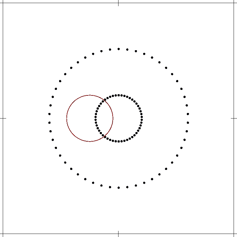
Fig. 1: Left: The solution $u^{\ast}(\mathbf{x})$ of the forward problem from which we generate “synthetic” measurements $z_{\ell}$ via (32). Right: The source term $q^{\ast}(\mathbf{x})$ from which we compute synthetic measurements is constant and nonzero only in the solid red circle offset from the center; the detector locations $\xi_{\ell},\ell=1,\ldots,L=100$ are marked by dots.

5.2 The inverse problem

The inverse problem we seek to solve is the identification of the source term $q(\mathbf{x})$ (which we approximate via a finite-dimensional expansion $\sum_{k}q_{k}s_{k}(\mathbf{x})$) in (30), based on the measurements described by (32). We approach this problem by reformulating it in the form of the constrained optimization problem (19), where we set the regularization parameter to $\beta=10^{4}$. This problem is then solved by introducing a Lagrangian

$${\mathfrak{L}}(u,q,\lambda)={\cal J}(u,q)+\int_{\Omega}\lambda(\mathbf{x})\left({\cal L}u(\mathbf{x})-q(\mathbf{x})\right)\text{d}x,$$

and then solving the linear system of partial differential equations that results by setting the derivatives of ${\mathfrak{L}}$ to zero (that is, the optimality conditions). In strong form, these optimality conditions read

$$\begin{split}{\cal L}u(\mathbf{x})&=q(\mathbf{x}),\\ {\cal L}^{\ast}\lambda(\mathbf{x})&=-\sum_{\ell}\frac{1}{\sigma^{2}_{\ell}}(u(\mathbf{\xi}_{\ell})-z_{\ell})\delta(\mathbf{x}-\mathbf{\xi}_{\ell}),\\ \beta q-\lambda&=0.\end{split}$$ (33)

The solution of this system of equations is facilitated by discretizing on a finite element mesh. We use continuous, piecewise cubic elements for $u$ and $\lambda$, and discontinuous, piecewise constants elements for $q$.

The three components $u,q,\lambda$ of this solution, computed on a very fine mesh with $256\times 256=$65\,536$$ cells, for which the coupled problem has $1\,248\,258$ unknowns, are shown in Fig. 2. The maximal value of the recovered source is less than half the maximal size of the “true” source, owing to the effect of the $L_{2}$ regularization term. As a consequence, the forward solution $u$ is also too small. Furthermore, the inverse problem places the source in a broader region than where it really is, but this is not surprising: In an advection-dominated problem, it is only possible to say with accuracy that the source is upstream of a detector, but not where in the upstream region it actually is unless another detector further upstream indicates that it must be downstream from the latter.

The adjoint variable $\lambda$ clearly illustrates the effect that the adjoint operator ${\cal L}^{\ast}$ transports information in the opposite direction $-\mathbf{b}$ of the forward operator ${\cal L}$, and that the sources of the adjoint equation are the residuals $-(u(\mathbf{\xi}_{\ell})-z_{\ell})\delta(\mathbf{x}-\mathbf{\xi}_{\ell})$; here $u(\mathbf{\xi}_{\ell})-z_{\ell}$ reflects the measurement error and, based on our choice of noise above, is Gaussian distributed with both positive and negative values.

The bottom right panel of the figure also shows the information density $j(\mathbf{x})$ that corresponds to this problem, as defined in (29). It illustrates that, given the location of detectors and the nature of the equation, information is primarily available upstream of detector locations. Notably, and as mentioned in Remark 4, the information density is based solely on the operator $\cal L$ and the measurement functionals $m_{\ell}$, but not on the actual measurements $z_{\ell}$ (or the noise that is part of $z_{\ell}$).

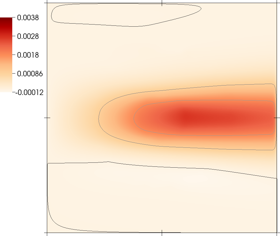
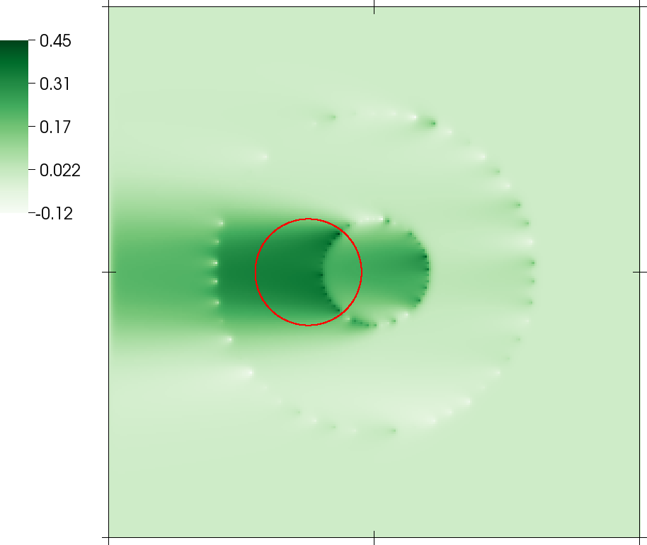
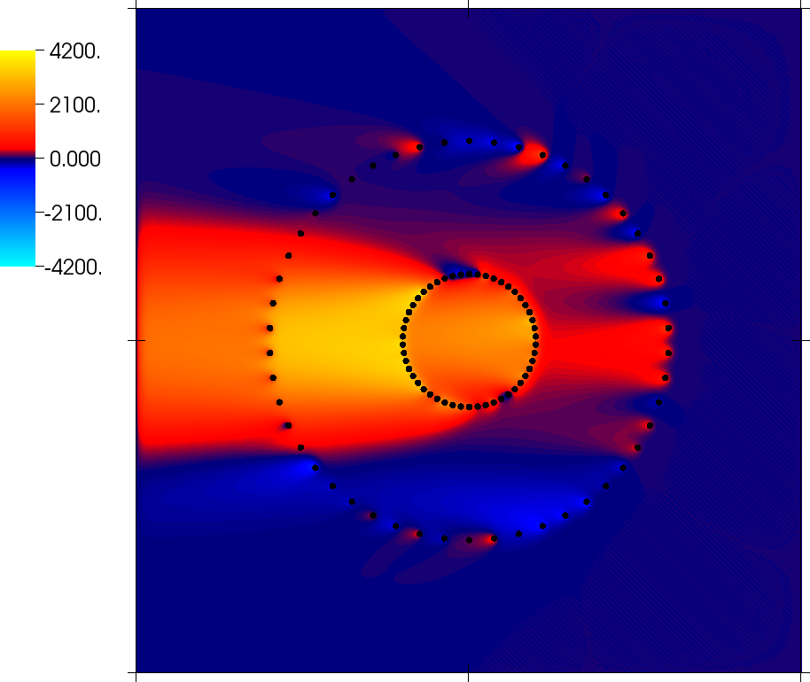
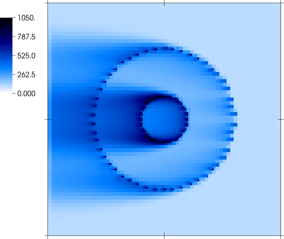
. $u(\mathbf{x})$ $q(\mathbf{x})$ .
. $\lambda(\mathbf{x})$ $j(\mathbf{x})$ .

Fig. 2: The solution of problem (33), computed on a very fine finite element mesh. Top left: The primal variable $u(\mathbf{x})$, shown with the same scale for color and isocontours as in Fig. 1. Top right: The recovered sources $q(\mathbf{x})$, i.e., the solution of the inverse problem. The red circle indicates the location of the source term used in generating the synthetic data. Bottom left: The adjoint variable $\lambda(\mathbf{x})$. Bottom right: The information density $j(\mathbf{x})$ associated with this problem, as defined in (29).

5.3 Choice of mesh for the inverse problem

The question of interest then is how we can use information densities for mesh refinement. To answer this question, we have repeated the computations discussed above, but instead of using a uniformly refined mesh, we have used a sequence of meshes in which we refine cells hierarchically so as to equilibrate the information content $j_{k}$ of each cell $\omega_{k}$, see (26), by always refining those cells that have the largest information content. The reconstructions and the sequence of meshes they are computed on are shown in Fig. 3. For comparison with the computations mentioned above and shown in Fig. 2, the rightmost mesh has $1642$ cells and the coupled problem solved on it has $32\,582$ unknowns.

.  

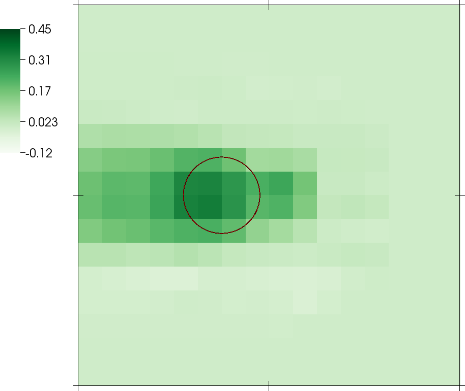
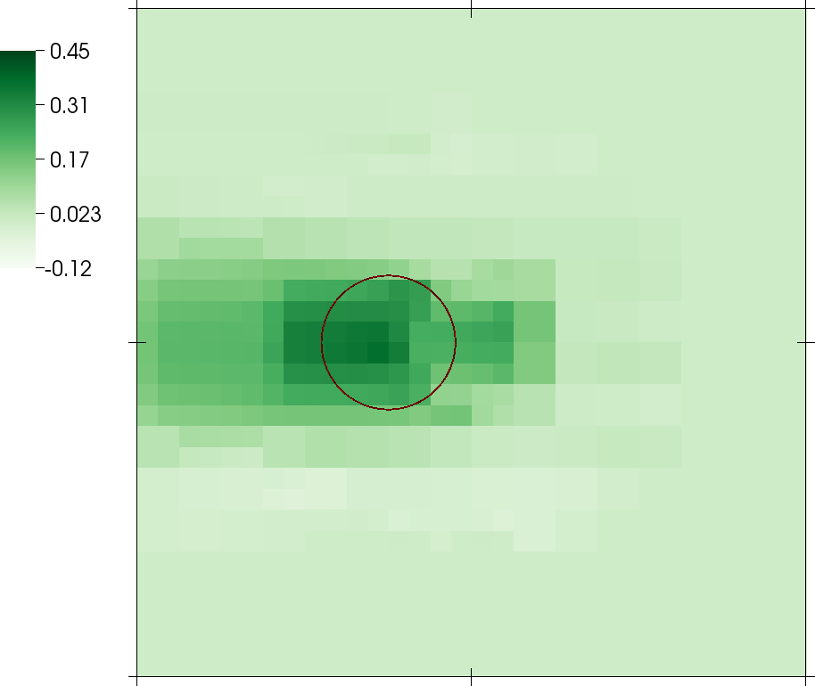
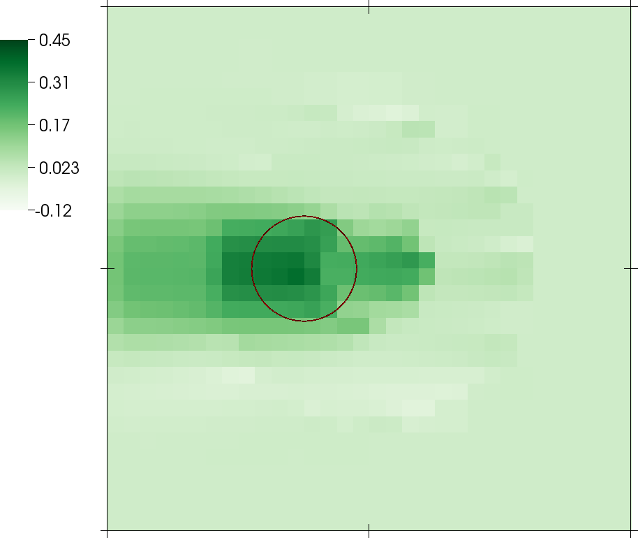
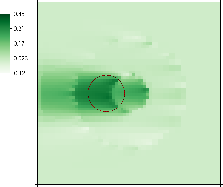
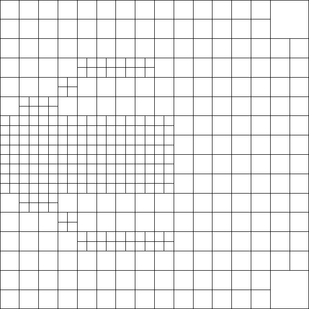
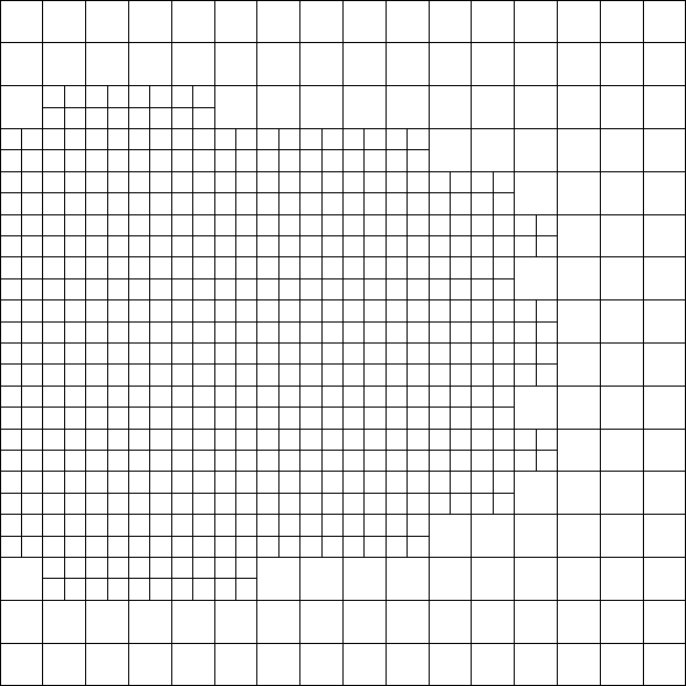
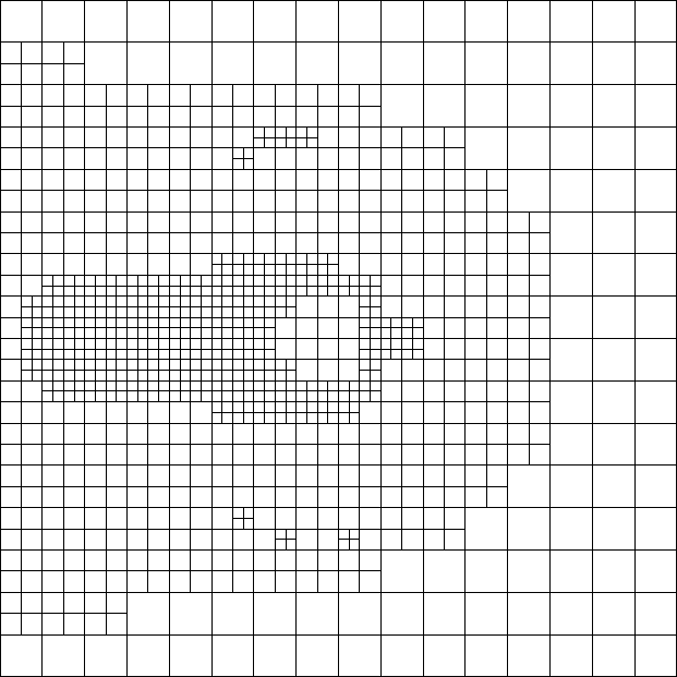
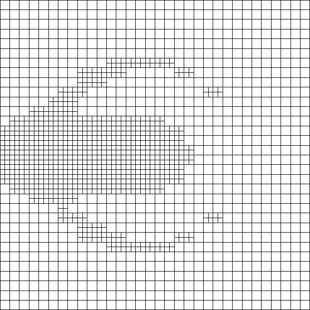
Fig. 3: Reconstructions (top) on a sequence of meshes (bottom) refined based on the information content of each cell of the mesh.

5.3.1 Comparison with other mesh refinement criteria

The relevant question to ask is whether this mesh is better suited to the task than any other potential mesh. Answering this question is notoriously difficult in inverse problems because, in general, the exact solution of the problem is unknown if only finitely many measurements are available and if regularization is used. As a consequence, it is difficult to answer the question through comparison of convergence rates of different methods, for example.

However, we can sometimes make intuitive comparisons based on experience on “how a good mesh should look”, even though for problems like the one under consideration, it is generally difficult to create such meshes by hand a priori. For comparison with the meshes shown in Fig. 3, we present in Fig. 4 the meshes generated using two different, “traditional” mesh refinement criteria that we will justify in more detail in Appendix B. In both cases, the meshes are obtained by always refining those cells $K$ that have the largest “refinement indicators” $\eta_{K}$. In the top row of Fig. 4, this indicator $\eta_{K}$ is the cell-wise norm of the residual of the third equation of (33) and is thus an a posteriori error indicator that can be derived in a way similar to that shown in [8, 10, 11, 31]:

$$\eta_{K}=\|\beta q-\lambda\|_{L_{1}(K)}.$$

We will consequently refer to this quantity as the “error estimator”.

In the bottom row of Fig. 4, we show meshes generated by evaluating a finite difference approximation $\nabla_{h}q(\mathbf{x})$ on each cell by comparing the values of $q|_{K}$ with the values of $q$ on neighboring cells, and then computing

$$\eta_{K}=h_{K}\|\nabla_{h}q\|_{L_{2}(K)},$$

where $h_{K}$ denotes the diameter of cell $K$. The choice of $\eta_{K}$ is proportional to the interpolation error of a continuous function when approximated by a piecewise constant finite element function (as we do here); the indicator therefore measures where the piecewise constant approximation is likely poor. We will refer to this criterion as the “smoothness indicator”. It is also used in [45], for example.

As outlined in Section 4.2, the literature contains discussions of many other ways to refine meshes for the inverse problem, but we consider the two mentioned above as representative mesh refinement criteria to compare our approach against. We provide a detailed derivation of these two indicators in Appendix B.

.  
.  

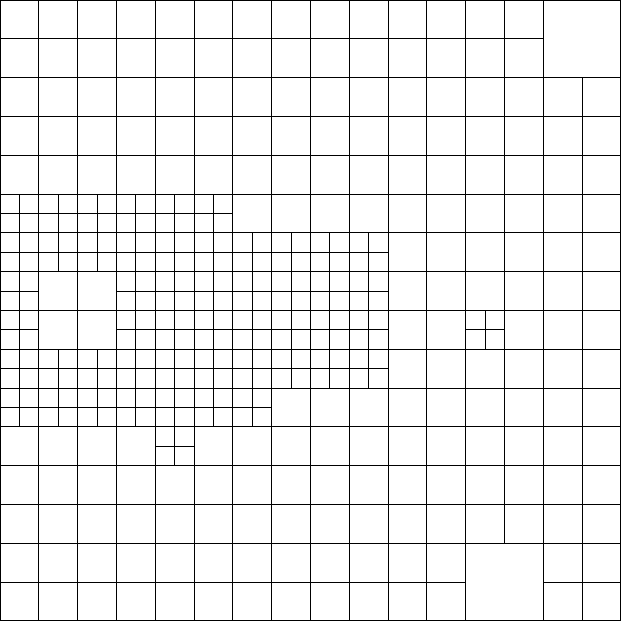
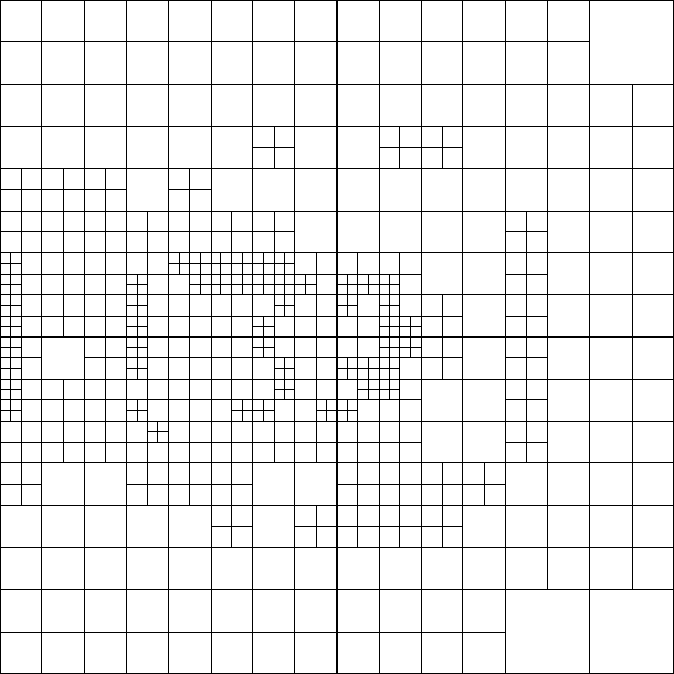
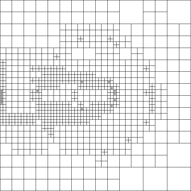
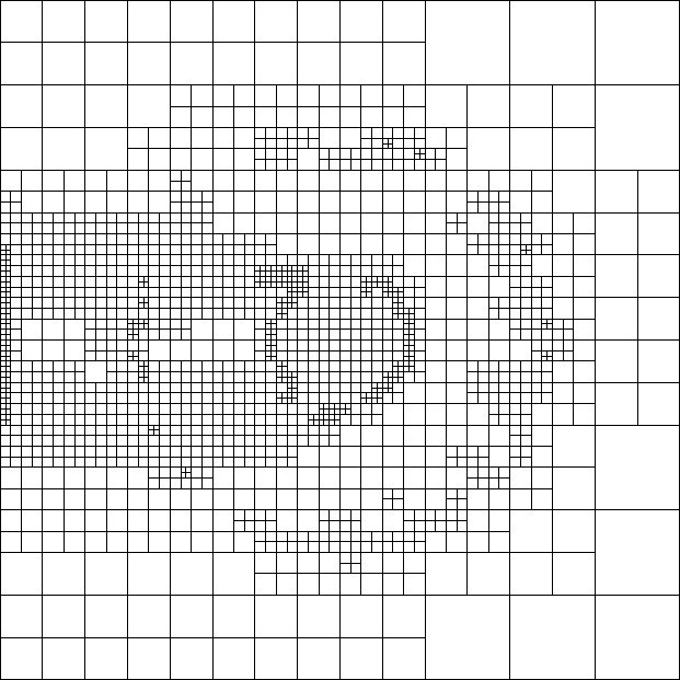
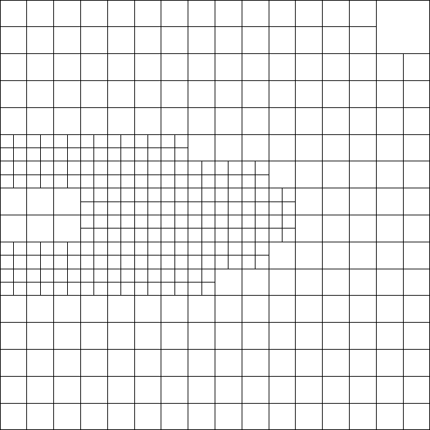
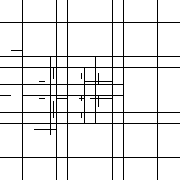
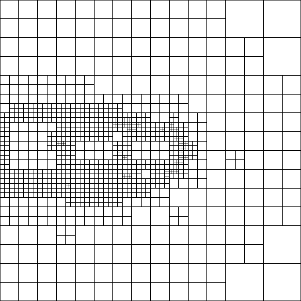
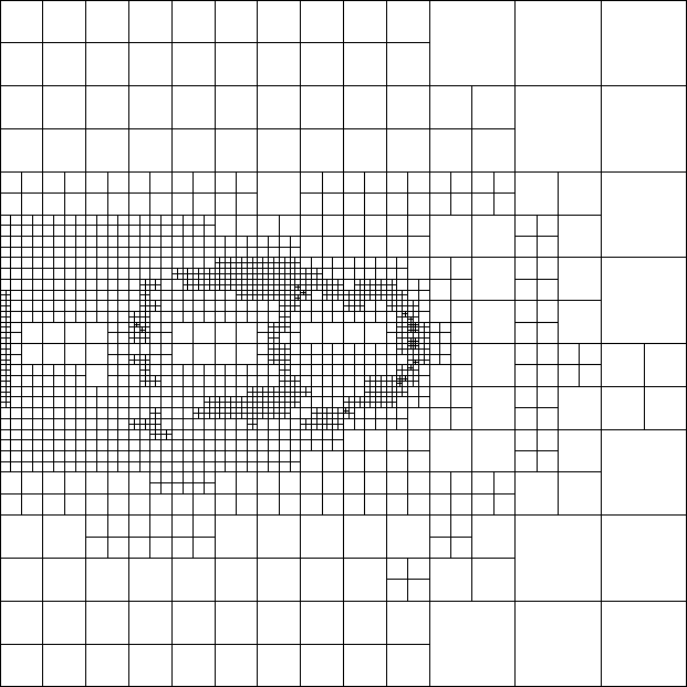
Fig. 4: Sequences of meshes generated by different mesh refinement criteria. Top: Mesh refinement is driven by an a posteriori error indicator. Bottom: Mesh refinement is driven by a a smoothness indicator.

The meshes shown in Fig. 4 are structurally similar to those generated based on the information content and shown in Fig. 3. However, they lack the top-bottom symmetry of the ones in Fig. 3 and look generally less organized, owing to the fact that they are based on the solution of the inverse problem, which is subject to the noise in the measurements, whereas the information density reflects only how much we know about the solution at a specific point in the domain – that is, a quantity that is independent of the concrete realization of the noise that is part of the measurements, see also Remark 4. Conceptually, the best mesh should be independent of the concrete realization of noise, although dependent on what is being measured. The refinement by information content allows us to construct the mesh even before solving the inverse problem because it does not depend on the solution of the inverse problem.

If the individual measurements $m_{\ell}$ had had differently sized measurement errors, then this would also have affected the information density-based mesh refinement and led to smaller cells where more accurate measurements are available. In contrast, there is no such direct dependence for the other refinement methods; rather, for those methods, variable noise levels only affect mesh refinement because $\lambda$ indirectly depends on the error level.

5.3.2 Quantitative evaluation: Condition numbers of matrices

A more concrete comparison between meshes would be to measure the degree of ill-posedness of the problem. Of course, we use regularization to make the problem well-posed, but a well-chosen mesh results in a matrix after discretization that has a better condition number than a poorly chosen mesh, and for which the reconstruction is consequently less sensitive to noise. In practice, the condition number is a poor indicator since it considers only the largest and smallest eigenvalues; we hypothesize that a better criterion would be to ask how many “large” eigenvalues there are, and it is this criterion that we will consider below.

To test this hypothesis, let us consider the discretized version of (33). If we collect the degrees of freedom of a finite element discretization of $u$ into a vector $U$, and similarly those of $\lambda$ into a vector $\Lambda$ and those of $q$ into the vector $P$ (a symbol chosen to avoid confusion with the matrix $Q$ of Section 2), then (33) corresponds to the following system of linear equations after discretization by the finite element method:

$$\begin{split}AU&=BP,\\ A^{T}\Lambda&=-C(U-Z),\\ \beta NP-B^{T}\Lambda&=0.\end{split}$$ (34)

Here, the matrix $A$ corresponds to the discretized operator ${\cal L}=\mathbf{b}\cdot\nabla-D\Delta$ acting on the finite element space chosen to discretize the state and adjoint variables, and $N$ is the mass matrix on the finite element space chosen for the source $q$ – that is, on the set of piecewise constant functions $s_{k}(\mathbf{x})$ associated with the cells of the mesh. The matrix $B$ results from the product $B_{ik}=(\varphi_{i},s_{k})_{\Omega}$ between the shape functions for $u$ and $q$, and $C$ corresponds to terms of the form $C_{ij}=\sum_{\ell}\frac{1}{\sigma^{2}_{\ell}}\varphi_{i}(\mathbf{\xi}_{\ell})\varphi_{j}(\mathbf{\xi}_{\ell})$. By noting that the matrices $A$ and $N$ are invertible, we can reduce this system of equations to an equation for $P$ by repeated substitution to

$$HP =B^{T}A^{-1}CZ,$$ (35)

where the matrix $$H$$ is the Schur complement,

$$H =B^{T}A^{-T}CA^{-1}B+\beta N.$$ (36)

The matrix $H$, which is symmetric and at least positive semidefinite, thus relates the vector of measurements $Z$ to the vector of coefficients $P$ we would like to recover. $H$ can be thought of as the discretized counterpart to the matrix $Q$ in (8). Each eigenvalue of $H$ then corresponds to an eigenvector (“mode”) of the coefficient $q(\mathbf{x})$ we would like to recover. Moreover, large eigenvalues correspond to modes that are insensitive to noise, whereas small eigenvalues correspond to modes that are strongly affected by noise. As a consequence, we would like to aim for discretizations that result in many large and few small eigenvalues.

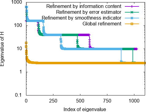
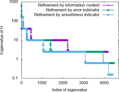
Fig. 5: Comparison of the eigenvalues of the resolution matrix $H$ for different ways of refining meshes. Left: After three refinement cycles, yielding problems with approximately 1,000 parameters to identify for the adaptive refinement criteria, and 16,384 for global refinement. For the global refinement case, only the first 1,100 eigenvalues are shown; the remaining ones have nearly the same value. Right: After six refinement cycles, resulting in problems with approximately 4,000 parameters for the adaptive refinement criteria. (Global refinement would have resulted in more than one million parameters; the eigenvalues of this matrix could not be computed.)

Fig. 5 provides a numerical evaluation of this perspective. It shows that when refining the mesh using the information content criterion, the eigenvalues of $H$ are further to the top right – in other words, there are more large eigenvalues than when using refinement by the error estimator or the smoothness indicator. This pattern persists after both three refinement cycles (the left part of the figure) and six refinement cycles (the right part).

The stair-step structure of the figure results from the fact that mesh refinement turns one large cell into four small ones. Consequently, in general one large eigenvalue turns into four smaller eigenvalues. By counting the number of derivatives present in the operators that enter into $H$, we can conjecture that the conditioning of the problem scales with the mesh size $h$ squared; indeed, the levels in the plots confirm that each mesh refinement step reduces the size of the smallest eigenvalues by approximately a factor of $(h_{\text{large}}/h_{\text{small}})^{2}=4$.

The left part of the figure also shows the eigenvalues of $H$ for meshes constructed via global refinement, where the globally refined mesh is chosen so that it has the same finest resolution as the adaptively refined ones. Global refinement results in vastly more unknowns than for the adaptively refined meshes, with a large majority of small eigenvalues. These eigenvalues all correspond to small cells to the right of the array of detectors where very little information is available. Given the size of the problem, we were not able to compute the eigenvalues of $H$ following six global refinement steps; the corresponding data are therefore omitted in the right panel.

The comparison shown in the figure confirms the hypothesis we laid out at the beginning of the section: namely, that refining the mesh based on information contents leads to an inverse problem that is better posed than those that result from any of the other refinement criteria we have compared with, in the sense that our approach leads to more large eigenvalues.

6 Conclusions and outlook

In this paper, we have used a statistical approach to define how much information we have about the parameter that is recovered in an inverse problem. More concretely, we have defined a density $j(\mathbf{x})$ that corresponds to how much we know about the solution at a given point $\mathbf{x}$, and derived an explicit expression for it that can be computed. We have then outlined a number of ways in which we believe that this information density can be used, via three vignettes. Finally, we have assessed one of these application areas numerically and showed that basing mesh refinement for inverse problems on information densities indeed leads to meshes that not only visually look more suited to the task than other criteria, but also quantitatively lead to better-posed discrete problems.

At the same time, this paper did not address many areas that would make for very natural next questions, including the following:

• In our work, we have chosen a simple $L_{2}$ regularization term $\frac{\beta}{2}\|q\|_{L_{2}}^{2}$, see (19). In practice, however, regularization terms would typically be used that penalize oscillations, for example using terms of the form $\frac{\beta}{2}\|\nabla^{\alpha}q\|_{L_{2}}^{2}$, $\alpha\geq 1$. How this would affect the definition of the information density would be interesting to ask in a future study. In order to consider the limit of infinite-dimensional inverse problems, we need to ensure that the covariance operators that result from regularization are of trace class (see, for example, [47, 1, 20]), which is also likely a precondition for the definition of information densities.

• For many inverse problems – such as ultrasound or seismic imaging, or electrical impedance tomography – the quantity we would like to identify is not a right-hand source term, but a coefficient in the operator on the left side of the equation. In these cases, the definition of the information density will have to be linearized around the solution of the inverse problem, which then may make the definition of $j(\mathbf{x})$ dependent on actual noise values. How this affects the usefulness of the information density is a priori unclear, but it would at least require solving the inverse problem before we can compute $j(\mathbf{x})$. We provide a brief outlook at this case in Appendix A.

• The computation of $j(\mathbf{x})$ requires the solution of a number of forward or adjoint problems, which is expensive, especially for three-dimensional inverse problems, even though these problems are all independent of each other and can be computed in parallel. At the same time, although we have shown in Sections 2 and 3 what is necessary to form the complete matrix $Q$, we need only the diagonal entries of this matrix, see (3.3). We may be able to compute approximations to the entries $Q_{kk}$ more cheaply, for example by random projections, low-rank approximations, or hierarchical low-rank approximations. Such ideas can, for example, be found in [24, 25, 1], and in [20, Section 5] and [2] for the closely related reduced Hessian matrix.

We leave the exploration of these topics to future work.

Acknowledgments.

WB would like to thank Dustin Steinhauer for an introduction to the Fisher information matrix many years ago. WB’s work was partially supported by the National Science Foundation under award OAC-1835673; by award DMS-1821210; and by award EAR-1925595. CRJ’s work was partially supported by the Intel Graphics and Visualization Institutes of XeLLENCE, the National Institutes of Health under award R24 GM136986, the Department of Energy under grant number DE-FE0031880, and the Utah Office of Energy Development.

This paper describes objective technical results and analysis. Any subjective views or opinions that might be expressed in the paper do not necessarily represent the views of the U.S. Department of Energy or the United States Government. Sandia National Laboratories is a multimission laboratory managed and operated by National Technology and Engineering Solutions of Sandia LLC, a wholly owned subsidiary of Honeywell International, Inc., for the U.S. Department of Energy’s National Nuclear Security Administration under contract DE-NA-0003525.

Appendix A On the extension to nonlinear problems

The derivations in both Section 2 (for the finite-dimensional case) and Section 3 (for the infinite-dimensional case) have assumed that the forward model is linear, and that the solution-to-measurement map is as well. This linearity is clearly a severe restriction – many inverse problems are nonlinear: typical examples are optical tomography, ultrasound imaging, electrical impedance tomography, or seismic imaging. In all of these cases, we seek to identify a coefficient inside a differential operator.

In order to understand what needs to change in the formalism we have outlined in this paper to accommodate the nonlinear case, we stay with the finite-dimensional case for simplicity; the infinite-dimensional case will follow the exact same steps. The argument is essentially one of linearization, predicated on the assumption that measurement errors are small and that the parameter-to-measurement map is sufficiently smooth.

First, let us assume that we replace the forward model (4) by the following model that is (potentially) nonlinear in the parameters $q_{k}$ we seek:

$$A(S\mathbf{q};\mathbf{u})=\mathbf{f},$$ (37)

where $S\mathbf{q}$ is a vector of coefficients that appear in the operator and is expressed in terms of a basis encoded by the columns of the matrix $S$ times the unknown parameters $\mathbf{q}$ we would like to identify. We have also allowed for a right-hand side forcing term $\mathbf{f}$ that is assumed known and that could have been incorporated into $A$ but commonly is not. For a given $\mathbf{q}$, we then use the following notation to denote the solution of the forward model:

$$\mathbf{u}=A(S\mathbf{q};\bullet)^{-1}\mathbf{f}.$$ (38)

Next, we assume that we obtain measurements using (possibly nonlinear) functionals $m_{\ell}$ instead of the linear ones in (5):

$$z_{\ell}=m_{\ell}(\mathbf{u})+\varepsilon_{\ell}.$$ (39)

We can combine the state equation and the measurement process by introducing the parameter-to-measurement map $\mathbf{F}(S\mathbf{q})$:

$$z_{\ell}=F(S\mathbf{q})_{\ell}+\varepsilon_{\ell}.$$ (40)

For comparison with the material in Section 2, note that in the linear case, we have that $A(S\mathbf{q};\mathbf{u})=A\mathbf{u}-S\mathbf{q}$, $\mathbf{f}=0$, $A(S\mathbf{q};\bullet)^{-1}\mathbf{f}=A^{-1}S\mathbf{q}$, and $\mathbf{F}(S\mathbf{q})=MA^{-1}S\mathbf{q}$.

With this parameter-to-measurement operator $\mathbf{F}$, the deterministic parameter estimation problem (7) then takes on the following form:

$$\min_{\mathbf{q}}\;{\cal J}_{\text{red}}(\mathbf{q}):= \underbrace{\frac{1}{2}\left\|\mathbf{F}(S\mathbf{q})-\mathbf{z}\right\|^{2}_{\Sigma^{-2}}+\frac{\beta}{2}\left\|R\mathbf{q}\right\|^{2}}_{=:{\cal J}_{\text{red}}(\mathbf{q}}.$$ (41)

Let us assume that this problem has a unique minimizer, which we will denote by $\mathbf{q}^{\ast}=\mathbf{q}^{\ast}(\mathbf{z})$. Then, under appropriate smoothness assumptions, we can perform a Taylor expansion of the optimality conditions for $\mathbf{q}^{\ast}$. For two random noisy realizations of measurements $\mathbf{z}_{1},\mathbf{z}_{2}$, we obtain that the minimizers $\mathbf{q}_{1}=\mathbf{q}(\mathbf{z}_{2}),\mathbf{q}_{2}=\mathbf{q}(\mathbf{z}_{2})$ of (41) have to satisfy the following relationship that generalizes (9):

$$Q(\mathbf{q}_{1}-\mathbf{q}_{2})=S^{T}F^{\prime}(S\mathbf{q}^{\ast})^{T}\Sigma^{-2}(\mathbf{z}_{1}-\mathbf{z}_{2})+{\cal O}(\|\mathbf{z}_{1}-\mathbf{z}\|^{2})+{\cal O}(\|\mathbf{z}_{2}-\mathbf{z}\|^{2}).$$ (42)

Here, the matrix $F^{\prime}(S\mathbf{q}^{\ast})$ is the derivative of the vector function $\mathbf{F}$ with regard to its argument, evaluated at $S\mathbf{q}^{\ast}$. In the linear case, $F^{\prime}=MA^{-1}$ is independent of $q^{\ast}$. The matrix $Q$ above readily generalizes the situation for the linear case and has the form:

$$Q=S^{T}F^{\prime}(S\mathbf{q}^{\ast})^{T}\Sigma^{-2}F^{\prime}(S\mathbf{q}^{\ast})S+\beta R^{T}R.$$ (43)

Ultimately, the information content we seek is based on the precision matrix, which we obtain via the Fisher information matrix from the Bayesian inverse problem (11). Specifically, we will continue to define the information content via the square root of the inverse of the diagonal elements of the covariance matrix (13), which we approximate by way of the Cramér-Rao bound and using (14):

$$j_{k}:=\sqrt{(I_{p})_{kk}},\qquad\text{ where }(I_{p})_{kk}={\mathbb{E}}\left[\frac{\partial^{2}}{\partial q_{k}^{2}}{\cal J}_{\text{red}}(\mathbf{q})\right]$$ (44)

The differences between the linear and nonlinear cases appear here. First, in the linear case, the Cramér-Rao bound holds with equality, and as a consequence the definition of $j_{k}$ in the previous equation also satisfies the desired identity (12)

$$j_{k}:=\sqrt{(I_{p})_{kk}}=\frac{1}{\sqrt{\text{var}_{p}(\mathbf{q})_{k}}}.$$

However, in the nonlinear case, the probability distribution $p(\mathbf{q}|\mathbf{z})$ is no longer Gaussian (because ${\cal J}_{\text{red}}$ is no longer quadratic in $\mathbf{q}$), and consequently the last identity of the previous equation may no longer be exact.

Second, in the linear case, we had $I_{p}=Q$ because ${\cal J}_{\text{ref}}({\mathbf{q}})$ is a quadratic function, its second derivative is a constant, $\frac{\partial^{2}}{\partial q_{k}\partial q_{l}}{\cal J}_{\text{red}}(\mathbf{q})=Q_{kl}$, and consequently the expectation value in (44) simply evaluates to $Q_{kk}$. In the nonlinear case, a straightforward Taylor expansion of the definition of ${\cal J}_{\text{red}}$ around $\mathbf{q}^{\ast}$ shows that to first order in $\mathbf{q}-\mathbf{q}^{\ast}$,

$$I_{p}\approx Q+\text{sym}\left((\mathbf{F}(S\mathbf{q}^{\ast})-\mathbf{z})^{T}\Sigma^{-2}F^{\prime\prime}(S\mathbf{q}^{\ast})SS\right)+\text{higher order terms},$$

with appropriate contractions over the indices of the various matrices and vectors that appear in this expression. Here, $\text{sym}(X)=\frac{1}{2}(X+X^{T})$ symmetrizes the matrix $X$.

The first correction term beyond $Q$ in the previous expression corresponds to the difference between the Gauss-Newton and Newton matrices in least-squares minimization [39]. The correction is small if either the problem is nearly linear ($F^{\prime\prime}$ is small), or if the residual $\mathbf{F}(S\mathbf{q}^{\ast})-\mathbf{z}$ is small – essentially a condition on whether the model is able to accurately predict the data and whether the noise level is small.

The next order term of the higher order corrections in the expression above is of the form ${\mathbb{E}}\left[\text{sym}\left(P(\mathbf{q}-\mathbf{q}^{\ast})\right)\right]=\text{sym}\left(P\;{\mathbb{E}}\left[\mathbf{q}-\mathbf{q}^{\ast}\right]\right)$, where $P$ is a rank-3 tensor composed of a lengthy list of terms proportional to at least second derivatives of $\mathbf{F}$, often multiplied by the residual $\mathbf{F}(S\mathbf{q}^{\ast})-\mathbf{z}$. As above, for problems that either have a small residual or are nearly linear, $P$ by itself is already small. Furthermore, if the noise level is small, we should expect the posterior probability to be localized near $\mathbf{q}^{\ast}$, nearly symmetric around $\mathbf{q}^{\ast}$, and therefore for the expectation value ${\mathbb{E}}\left[\mathbf{q}-\mathbf{q}^{\ast}\right]$ to be small.

Whether or not these correction terms will be small for a concrete application depends, of course, on both how nonlinear the operator $\mathbf{F}$ is (i.e., how large $\mathbf{F}^{\prime\prime}$ is) and how large we expect the measurement errors (and consequently the residuals) to be. Assuming that one or the other is indeed small for a particular case, it seems reasonable to expect that our choice (16) for the information content, namely

$$j_{k}:=\sqrt{Q_{kk}},$$

may still be a useful one for nonlinear problems.

Having settled the question of how to define the information content $j_{k}$ in the nonlinear case, there remains the question of how to compute it. Given (43), we find that it can be computed in much the same way as outlined in Section 2.2, Remark 1. In analogy to the derivations there, note that now

$$Q_{kk} =\mathbf{e}_{k}^{T}S^{T}F^{\prime}(S\mathbf{q}^{\ast})^{T}\Sigma^{-2}F^{\prime}(S\mathbf{q}^{\ast})S\mathbf{e}_{k}+\beta\mathbf{r}_{k}^{T}\mathbf{r}_{k}$$

$$=\left(\Sigma^{-1}F^{\prime}(S\mathbf{q}^{\ast})S\mathbf{e}_{k}\right)^{T}\left(\Sigma^{-1}F^{\prime}(S\mathbf{q}^{\ast})S\mathbf{e}_{k}\right)+\beta\mathbf{r}_{k}^{T}\mathbf{r}_{k}$$

$$=\sum_{\ell}\frac{1}{\sigma_{\ell}^{2}}\eta_{\ell k}^{2}+\beta\mathbf{r}_{k}^{T}\mathbf{r}_{k},$$

where

$$\eta_{\ell k}=F_{\ell}^{\prime}(S\mathbf{q}^{\ast})S\mathbf{e}_{k}.$$

These quantities require a solve with the linearized forward model, linearized around the solution $\mathbf{q}^{\ast}$ of the deterministic problem. Similar considerations apply when computing $Q_{kk}$ via adjoint solutions (the “alternative way” in Remark 1).

The cost of these forward solves is the same as for the linear case, but two other considerations come into play. First, the solution of the nonlinear inverse problem problem (in which we are of course primarily interested) is generally more expensive than for linear problems, and so the cost of computing information contents $j_{k}$ may or may not be a major cost any more, unlike in the linear case. On the other hand, in the nonlinear case, the definition of $Q_{kk}$ and consequently $j_{k}$ depends on the solution $\mathbf{q}^{\ast}$ of the deterministic problem and, thus, on the noisy data $\mathbf{z}$ from which $\mathbf{q}^{\ast}$ was computed. This is unfortunate: One of the major benefits of using $j_{k}$ touted in Remark 4 was that it did not depend on the noisy data, unlike all other criteria we know of. Whether this dependence is strong enough in practice to be important will remain an open question for now; as in the discussions about the difference between $Q$ and $I_{p}$, we can speculate that this is a higher order concern, unlike for example in the mesh refinement criteria in Fig. 4, where the noise in the data was clearly visible in the structure of the generated mesh.

Appendix B On the derivation of traditional mesh refinement criteria

Section 5.3.1 contains a comparison of our information-density based mesh refinement criterion against two other mesh refinement criteria that we have called “error estimator” and “smoothness indicator”. Both of these can be derived in ways that follow common finite element theory. In the following, we will attempt to provide an intuitive derivation of their form, without attempting to be precise and complete.

The starting point for the derivation of both forms is the optimality condition (33) – a system of partial differential equations – for the deterministic problem we are trying to solve. For simplicity, let us repeat this set of equations here:

$${\cal L}u(\mathbf{x}) =q(\mathbf{x}),$$

$${\cal L}^{\ast}\lambda(\mathbf{x}) =-\sum_{\ell}\frac{1}{\sigma^{2}_{\ell}}(u(\mathbf{\xi}_{\ell})-z_{\ell})\delta(\mathbf{x}-\mathbf{\xi}_{\ell}),$$

$$\beta q-\lambda =0.$$

In order to compute a numerical solution, we seek finite-dimensional approximations $u_{h}(\mathbf{x}),\lambda_{h}(\mathbf{x}),q_{h}(\mathbf{x})$ of the exact solution $u(\mathbf{x}),\lambda(\mathbf{x}),q(\mathbf{x})$ of this problem. We will use the finite element method; specifically, we will use piecewise polynomials of degree $p_{u},p_{\lambda},p_{q}$ for this approximation. The appropriate choice in the current context is to use continuous shape functions for $u_{h}$ and $\lambda_{h}$ (because we apply a second-order differential operator, for which the weak form of the equations above requires $H^{1}$ solutions of which the continuous functions are a subset), and discontinuous shape functions for $q_{h}$ (because no differential operator is ever applied to this variable).

To assess the quality of the mesh we have chosen, we would like to quantify the “error”, i.e., the difference between $u$ and $u_{h}$, and similarly for the other variables. For the second order operator $\cal L$ we consider, the appropriate norm to measure this error is

$$e:=\left(\|\nabla(u-u_{h})\|^{2}_{L^{2}(\Omega)}+\|\nabla(\lambda-\lambda_{h})\|^{2}_{L^{2}(\Omega)}+\|q-q_{h}\|^{2}_{L^{2}(\Omega)}\right)^{1/2}.$$ (45)

There are now two conceptually different ways in which we can approach estimating this error: a priori and a posteriori error estimates. These two approaches will yield the two criteria we used in Section 5.3.1.

A priori error estimates are based on the premise that for many equations and under certain conditions, one can show that on every cell $K$ of the mesh, we have [18, 19]

$$\|\nabla(u-u_{h})\|_{L^{2}(K)} \leq c_{u}\|\nabla(u-I_{h,p_{u}}u)\|_{L^{2}(K)} \leq C_{u}h_{K}^{p_{u}}\|\nabla^{p_{u}+1}u\|_{L^{2}(K)},$$

$$\|\nabla(\lambda-\lambda_{h})\|_{L^{2}(K)} \leq c_{\lambda}\|\nabla(\lambda-I_{h,p_{\lambda}}\lambda)\|_{L^{2}(K)} \leq C_{\lambda}h_{K}^{p_{\lambda}}\|\nabla^{p_{\lambda}+1}u\|_{L^{2}(K)},$$

$$\|q-q_{h}\|_{L^{2}(K)} \leq c_{q}\|q-I_{h,q_{q}}u\|_{L^{2}(K)} \leq C_{q}h_{K}^{p_{q}}\|\nabla^{p_{q}+1}u\|_{L^{2}(K)},$$

where $c_{\bullet},C_{\bullet}<\infty$ are constants we know exist but generally do not know the value of, and $I_{h,p}$ denotes the interpolation operator from a function to a discrete, piecewise polynomial function represented on the mesh with polynomial degree $p$. The first inequality in each line above represents the “best-approximation” property that holds for many equations and finite element schemes, whereas the latter is the Bramble-Hilbert inequality for polynomial approximation. $h_{K}$ denotes the diameter of cell $K$.

Because we were primarily interested in the mesh used to discretize the coefficient $q$ in Section 5.3, we chose $p_{u}=p_{\lambda}=3,p_{q}=0$. In other words, we used cubic elements to represent $u,\lambda$ accurately, but approximated $q$ only with piecewise constant functions. With the considerations above, the a priori error estimate (45) would then have the form

$$e =\left(\sum_{K}\left[\|\nabla(u-u_{h})\|^{2}_{L^{2}(K)}+\|\nabla(\lambda-\lambda_{h})\|^{2}_{L^{2}(K)}+\|q-q_{h}\|^{2}_{L^{2}(K)}\right]\right)^{1/2}$$

$$\leq C\left(\sum_{K}\left[h_{K}^{6}\|\nabla^{4}u\|_{L^{2}(K)}^{2}+h_{K}^{6}\|\nabla^{4}\lambda\|_{L^{2}(K)}^{2}+h_{K}^{2}\|\nabla q\|_{L^{2}(K)}^{2}\right]\right)^{1/2}$$

$$\approx C\left(\sum_{K}h_{K}^{2}\|\nabla q\|_{L^{2}(K)}^{2}\right)^{1/2}.$$

The last approximation is because for sufficiently small $h_{K}$, the first two terms in square brackets are much smaller than the third because their exponents are much larger. In practice, the exact solution $q$ is of course unknown, but we can derive a computable quantity for mesh refinement purposes by defining

$$\eta_{K}=h_{K}\|\nabla_{h}q_{h}\|_{L_{2}(K)}$$

for every cell, where $q_{h}$ is the computed approximate solution, and $\nabla_{h}q_{h}$ is a finite difference approximation of the gradient $\nabla q$ based on the piecewise constant function $q_{h}$. We have omitted the (unknown) constant $C$ because we are only interested in comparing which cells have large and which have small errors, rather than actually computing a reasonable approximation for $e$. This derivation of $\eta_{K}$ therefore leads to the “smoothness indicator” used in Section 5.3.1. The term “smoothness” indicates that we are measuring the size of derivatives of the function $(\mathbf{x})$.

The second approach toward deriving estimates for the error $e$, called “a posteriori error estimation”, is premised on first computing a numerical solution $u_{h},\lambda_{h},q_{h}$ and then deriving an estimate for $e$ that does not require knowledge of the true solution $u,\lambda,q$. Omitting many details (but see [11, 51]), we typically end up with an estimate that contains norms of the residual (i.e., the degree to which the left and right hand sides of (33) are not actually equal), times a constant of again unknown size, times powers of the mesh size $h_{K}$ in the same way as above. That is, these error estimators will have the form

$$e \leq C\Biggl{\{}\sum_{K}\Biggl{[}h_{K}^{6}\left(\|{\cal L}u_{h}-q_{h}\|_{L^{2}(K)}^{2}+\text{jump}(u_{h})\right)$$

$$\qquad\qquad+h_{K}^{6}\left(\left\|{\cal L}^{\ast}\lambda_{h}+\sum_{\ell}\frac{1}{\sigma^{2}_{\ell}}(u(\mathbf{\xi}_{\ell})-z_{\ell})\delta(\mathbf{x}-\mathbf{\xi}_{\ell})\right\|_{L^{2}(K)}^{2}+\text{jump}(\lambda_{h})\right)$$

$$\qquad\qquad+h_{K}^{2}\|\beta q_{h}-\lambda_{h}\|_{L^{2}(K)}^{2}\Biggr{]}\Biggr{\}}^{1/2}$$

$$\approx C\left(\sum_{K}h_{K}^{2}\|\beta q_{h}-\lambda_{h}\|_{L^{2}(K)}^{2}\right)^{1/2}.$$

In these formulas, $\text{jump}(u_{h})$ and $\text{jump}(\lambda_{h})$ are “jump terms” that arise due to integration by parts and whose specific form is not important in the current context. Crucially, again for reasons of high powers of $h_{K}$, we can estimate $e$ in the last line by omitting everything but the term that contains the residual of the last line of the optimality conditions (33). Again dropping the unknown constant $C$ for the same reasons as above, we can define an indicator for the size of the error on cell $K$ by

$$\eta_{K}=h_{K}\|\beta q_{h}-\lambda_{h}\|_{L_{2}(K)}.$$

This is nearly the “error estimator” form of $\eta_{K}$ presented in Section 5.3.1 – the difference being that we use the $L_{1}$-norm instead of the $L_{2}$-norm above. We note that this derivation is essentially what all publications do that base their mesh refinement decisions on a posteriori error estimates, perhaps up to the choice of norm or using weighting factors derived from dual solutions (see, for example, [8, 11, 9, 31], along with many others). The estimator $\eta_{K}$ we use here is then really just a “redux” of what other papers use, adapted to the fact that we have chosen $p_{u},p_{\lambda}\gg p_{q}$.

The two choices for the refinement criterion $\eta_{K}$ we have derived in these ways thus represent the two most widely used ways to derive error estimators for finite element discretizations. There, of course, exists a large collection of publications that derive variations of such estimators, perhaps also including ways of assessing the sizes of the constants that appear in the estimates, but experience has shown that – at least for the purposes of mesh refinement – the meshes obtained from different estimators vary little and look conceptually very similar within each of the two broad categories of deriving these estimators. As a consequence, we consider the two choices we have presented here as representative for these categories, and we do not expect that any variation on the approach would produce meshes that are fundamentally better or worse. This, in particular, includes the methods presented in the papers mentioned in the previous paragraph. In contrast, the refinement indicator based on the information density is an entirely different approach that has no resemblance to either of the two methods outlined above – in fact, it makes no reference to any numerical solution of the optimality conditions at all!

References

- [1] A. Alexanderian, N. Petra, G. Stadler, and O. Ghattas, A-optimal design of experiments for infinite-dimensional Bayesian linear inverse problems with regularized -sparsification, SIAM Journal on Scientific Computing, 36 (2014), pp. A2122–A2148.
- [2] I. Ambartsumyan, W. Boukaram, T. Bui-Thanh, O. Ghattas, D. Keyes, G. Stadler, G. Turkiyyah, and S. Zampini, Hierarchical matrix approximations of Hessians arising in inverse problems governed by PDEs, SIAM J. Sci. Comput., 42 (2020), pp. A3397–A3426.
- [3] D. Arndt, W. Bangerth, B. Blais, M. Fehling, R. Gassmöller, T. Heister, L. Heltai, U. Köcher, M. Kronbichler, M. Maier, P. Munch, J.-P. Pelteret, S. Proell, K. Simon, B. Turcksin, D. Wells, and J. Zhang, The deal.II library, version 9.3, Journal of Numerical Mathematics, 29 (2021), pp. 171–186.
- [4] D. Arndt, W. Bangerth, D. Davydov, T. Heister, L. Heltai, M. Kronbichler, M. Maier, J.-P. Pelteret, B. Turcksin, and D. Wells, The deal.II finite element library: design, features, and insights, Computers & Mathematics with Applications, 81 (2021), pp. 407–422.
- [5] S. R. Arridge and M. Schweiger, Inverse methods for optical tomography, in Information Processing in Medical Imaging, Harrison H. Barrett and A. F. Gmitro, eds., Berlin, Heidelberg, 1993, Springer Berlin Heidelberg, pp. 259–277.
- [6] A. C. Atkinson and A. N. Donev, Optimum Experimental Design, Clarendon Press, Oxford, 1992.
- [7] L. Auer, L. Boschi, T. W. Becker, T. Nissen‐Meyer, and D. Giardini, Savani: A variable resolution whole‐mantle model of anisotropic shear velocity variations based on multiple data sets, J. Geophys. Res. Solid Earth, 119 (2014), pp. 3006–3034.
- [8] W. Bangerth, Adaptive Finite Element Methods for the Identification of Distributed Parameters in Partial Differential Equations, PhD thesis, University of Heidelberg, 2002.
- [9] , A framework for the adaptive finite element solution of large inverse problems, SIAM J. Sc. Comput., 30 (2008), pp. 2965–2989.
- [10] W. Bangerth and A. Joshi, Adaptive finite element methods for the solution of inverse problems in optical tomography, Inverse Problems, 24 (2008), p. 034011.
- [11] W. Bangerth and R. Rannacher, Adaptive Finite Element Methods for Differential Equations, Birkhäuser Verlag, 2003.
- [12] H. T. Banks, K. Holm, and F. Kappel, Comparison of optimal design methods in inverse problems, Inverse Problems, 27 (2011), p. 075002.
- [13] A. J. Berglund, Statistics of camera-based single-particle tracking, Physical Review E, 82 (2010).
- [14] J. G. Berryman, Analysis of approximate inverses in tomography in tomography I. Resolution analysis of common inverses, Optimization and Engineering, 1 (2000), pp. 87–115.
- [15] D. Bigoni, Y. Chen, N. Garcia Trillos, Y. Marzouk, and D Sanz-Alonso, Data-driven forward discretizations for Bayesian inversion, Inverse Problems, 36 (2020), p. 105008.
- [16] R. Bonadio, S. Lebedev, T. Meier, P. Arroucau, A. J. Schaeffer, A. Licciardi, M. R. Agius, C. Horan, L. Collins, B. M. O’Reilly, P. W. Readman, and Ireland Array Working Group, Optimal resolution tomography with error tracking and the structure of the crust and upper mantle beneath Ireland and Britain, Geophysical Journal International, 226 (2021), pp. 2158–2188.
- [17] L. Borcea, V. Druskin, and A. V. Mamonov, Circular resistor networks for electrical impedance tomography with partial boundary measurements, Inverse Problems, 26 (2010), pp. 045010/1–32.
- [18] D. Braess, Finite elements, Cambridge University Press, 1997.
- [19] S. C. Brenner and R. L. Scott, The Mathematical Theory of Finite Elements, Springer, Berlin-Heidelberg-New York, second ed., 2002.
- [20] T. Bui-Thanh, O. Ghattas, J. Martin, and G. Stadler, A computational framework for infinite-dimensional bayesian inverse problems part i: The linearized case, with application to global seismic inversion, SIAM J. Sci. Comput., 35 (2013), pp. A2494–A2523.
- [21] C. Cohen-Bacrie, Y. Goussard, and R. Guardo, Regularized reconstruction in electrical impedance tomography using a variance uniformization constraint, IEEE Trans. Med. Imag., 16 (1997), pp. 562–571.
- [22] T. M. Cover and J. A. Thomas, Elements of Information Theory, Wiley, 2006.
- [23] D. R. Cox and D. V. Hinkley, Theoretical Statistics, Chapman, 1974.
- [24] S. Das, Efficient calculation of Fisher information matrix: Monte Carlo approach using prior information, PhD thesis, Johns Hopkins University, 2007.
- [25] S. Das, J. C. Spall, and R. Ghanem, Efficient monte carlo computation of fisher information matrix using prior information, Computational Statistics & Data Analysis, 54 (2010), pp. 272–289.
- [26] A. Datta-Gupta, J. Xie, N. Gupta, M. J. King, and W. J. Lee, Radius of investigation and its generalization to unconventional reservoirs, J. Petroleum Techn., (2011), pp. 52–55.
- [27] M. H. DeGroot, Optimal statistical decisions, Wiley-Interscience, 1970.
- [28] A. F. Emery and A. V. Nenarokomov, Optimal experiment design, Measurement Science and Technology, 9 (1998), pp. 864–876.
- [29] H. W. Engl, M. Hanke, and A. Neubauer, Regularization of Inverse Problems, Kluwer Academic Publishers, Dordrecht, 1996.
- [30] Y. Favennec, Hessian and Fisher matrices for error analysis in inverse heat conduction problems, Numerical Heat Transfer, Part B: Fundamentals, 52 (2007), pp. 323–340.
- [31] A. Griesbaum, B. Kaltenbacher, and B. Vexler, Efficient computation of the Tikhonov regularization parameter by goal-oriented adaptive discretization, Inverse Problems, 24 (2008), p. 025025.
- [32] A. Jamshidi, J. M. V. Samani, H. M. V. Samani, A. Zanini, M. G. Tanda, and M. Mazaheri, Solving inverse problems of unknown contaminant source in groundwater-river integrated systems using a surrogate transport model based optimization, Water, 12 (2020).
- [33] J. Kaipio and E. Somersalo, Statistical and Computational Inverse Problems, Springer, 2006.
- [34] S. M. Kay, Fundamentals of Statistical Signal Processing, Volume I: Estimation Theory, Prentice Hall, 1993.
- [35] F. J. Kuchuk, Radius of investigation for reserve estimation from pressure transient well tests, SPE, (2009), pp. 120515/1–22.
- [36] Q. Liu and Y. J. Gu, Seismic imaging: From classical to adjoint tomography, Tectonophysics, 566-567 (2012), pp. 31–66.
- [37] R. Montelli, G. Nolet, F. A. Dahlen, and G. Masters, A catalogue of deep mantle plumes: New results from finite-frequency tomography, Geochemistry, Geophysics, Geosystems, 7 (2006), pp. n/a–n/a.
- [38] R. M. Neupauer, B. Borchers, and J. L. Wilson, Comparison of inverse methods for reconstructing the release history of a groundwater contamination source, Water Resources Research, 36 (2000), pp. 2469–2475.
- [39] J. Nocedal and S. J. Wright, Numerical Optimization, Springer Series in Operations Research, Springer, New York, 1999.
- [40] S. Nordebo and M. Gustavsson, A priori modeling for gradient based inverse scattering algorithms, Progress in Electromagnetics Research B, 16 (2009), pp. 407–432.
- [41] B. W. Pogue, T. O. McBride, J. Prewitt, U. L Österberg, and K. D. Paulsen, Spatially variant regularization improves optical tomography, Appl. Optics, 38 (1999), pp. 2950–2961.
- [42] N. Rawlinson, A. Fichtner, M. Sambridge, and M. K. Young, Seismic tomography and the assessment of uncertainty, in Advances in Geophysics, Elsevier, 2014, pp. 1–76.
- [43] J. Ritsema, A. Deuss, H. J. van Heijst, and J. H. Woodhouse, S40RTS: a degree-40 shear-velocity model for the mantle from new rayleigh wave dispersion, teleseismic traveltime and normal-mode splitting function measurements, Geophysical Journal International, 184 (2010), pp. 1223–1236.
- [44] E. Romera, P. Sánchez-Moreno, and J. S. Dehesa, The Fisher information of single-particle systems with a central potential, Chemical Physics Letters, 414 (2005), pp. 468–472.
- [45] M. Sambridge and N. Rawlinson, Seismic tomography with irregular meshes, in Seismic earth: Array analysis of broadband seismograms, A. Levander and G. Nolet, eds., American Geophysical Union, 2005, pp. 49–65.
- [46] T. H. Skaggs and Z. J. Kabala, Recovering the release history of a groundwater contaminant, Water Resources Research, 30 (1994), pp. 71–79.
- [47] A. M. Stuart, Inverse problems: A Bayesian perspective, Acta Numerica, 19 (2010), pp. 451–559.
- [48] L. Tang, G. Hamarneh, and R. Abugharbieh, Reliability-driven, spatially-adaptive regularization for deformable registration, in Biomedical Image Registration, 4th International Workshop, WBIR 2010, Lübeck, Germany, July 11-13, 2010. Proceedings, B. Fischer, B. M. Dawant, and C. Lorenz, eds., vol. 6204 of Lecture Notes in Computer Science, Springer, 2010, pp. 173–185.
- [49] A. Tarantola, Inverse Problem Theory and Methods for Model Parameter Estimation, SIAM, 2004.
- [50] D. W. Vasco, H. Keers, and K. Karasaki, Estimation of reservoir properties using transient pressure data: An asymptotic approach, Water Resources Res., 36 (2000), pp. 3447–3465.
- [51] R. Verfürth, A Review of A Posteriori Error Estimation and Adaptive Mesh Refinement Techniques, Wiley/Teubner, New York, Stuttgart, 1996.
- [52] J. A. Vrugt, P. H. Stauffer, T. Wöhling, B. A. Robinson, and V. V. Vesselinov, Inverse Modeling of Subsurface Flow and Transport Properties: A Review with New Developments, Vadose Zone Journal, 7 (2008), pp. 843–864.
- [53] M. W. Woolrich, T. E. J. Behrens, C. F. Beckmann, and S. M. Smith, Mixture models with adaptive spatial regularization for segmentation with an application to MRI, IEEE Trans. Med. Imag., 24 (2005), pp. 1–11.
- [54] Y. Yin, E. A. Hoffman, and C.-L. Lin, Lung lobar slippage assessed with the aid of image registration, Med. Image. Comput. Comput. Assist. Interv., 13 (2010), pp. 578–585.
- [55] H. Zhang and C. H. Thurber, Estimating the model resolution matrix for large seismic tomography problems based on lanczos bidiagonalization with partial reorthogonalization, Geophysical Journal International, 170 (2007), pp. 337–345.