\externaldocument
[main-]dasf_part2_ieee
A Unified Algorithmic Framework for Distributed Adaptive Signal and Feature Fusion Problems
— Part II: Convergence Properties: Supplementary Material
Cem Ates Musluoglu, Charles Hovine,
and Alexander Bertrand
Copyright ©2023 IEEE. Personal use of this material is permitted. Permission from IEEE must be obtained for all other uses, in any current or future media, including reprinting/republishing this material for advertising or promotional purposes, creating new collective works, for resale or redistribution to servers or lists, or reuse of any copyrighted component of this work in other works.This paper is a supplementary material to [1 ] .
This supplementary material details the steps we follow to prove Lemma LABEL:main-lem:rank_H from [1 ] , i.e., to show that rank ( 𝐇 ) = K J − J rank 𝐇 𝐾 𝐽 𝐽 \text{rank}(\mathbf{H})=KJ-J 𝐇 ⋅ 𝝀 𝒦 = 0 ⋅ 𝐇 subscript 𝝀 𝒦 0 \mathbf{H}\cdot\bm{\lambda}_{\mathcal{K}}=0 LABEL:main-eq:H_lambda_0 ) in [1 ] ) can only have solutions 𝝀 𝒦 = [ 𝝀 T ( 1 ) , … , 𝝀 T ( K ) ] T subscript 𝝀 𝒦 superscript superscript 𝝀 𝑇 1 … superscript 𝝀 𝑇 𝐾
𝑇 \bm{\lambda}_{\mathcal{K}}=[\bm{\lambda}^{T}(1),\dots,\bm{\lambda}^{T}(K)]^{T} 𝝀 ( 1 ) = ⋯ = 𝝀 ( K ) 𝝀 1 ⋯ 𝝀 𝐾 \bm{\lambda}(1)=\dots=\bm{\lambda}(K) LABEL:main-cond:lin_indep_2 (repeated below) is satisfied.
Condition LABEL:main-cond:lin_indep_2 .
For a fixed point \macc@depth Δ \frozen@everymath \macc@group \macc@set@skewchar \macc@nested@a 111 X \macc@depth Δ \frozen@everymath \macc@group \macc@set@skewchar \macc@nested@a 111 𝑋 \macc@depth\char 1\relax\frozen@everymath{\macc@group}\macc@set@skewchar\macc@nested@a 111{X} LABEL:main-alg:dasf , the elements of the set { D j , q ( \macc@depth Δ \frozen@everymath \macc@group \macc@set@skewchar \macc@nested@a 111 X ) } j ∈ 𝒥 subscript subscript 𝐷 𝑗 𝑞
\macc@depth Δ \frozen@everymath \macc@group \macc@set@skewchar \macc@nested@a 111 𝑋 𝑗 𝒥 \{D_{j,q}(\macc@depth\char 1\relax\frozen@everymath{\macc@group}\macc@set@skewchar\macc@nested@a 111{X})\}_{j\in\mathcal{J}} q 𝑞 q
D j , q ( \macc@depth Δ \frozen@everymath \macc@group \macc@set@skewchar \macc@nested@a 111 X ) = [ \macc@depth Δ \frozen@everymath \macc@group \macc@set@skewchar \macc@nested@a 111 X q T ∇ X q h j ( \macc@depth Δ \frozen@everymath \macc@group \macc@set@skewchar \macc@nested@a 111 X ) ∑ k ∈ ℬ n 1 q \macc@depth Δ \frozen@everymath \macc@group \macc@set@skewchar \macc@nested@a 111 X k T ∇ X k h j ( \macc@depth Δ \frozen@everymath \macc@group \macc@set@skewchar \macc@nested@a 111 X ) ⋮ ∑ k ∈ ℬ n | 𝒩 q | q \macc@depth Δ \frozen@everymath \macc@group \macc@set@skewchar \macc@nested@a 111 X k T ∇ X k h j ( \macc@depth Δ \frozen@everymath \macc@group \macc@set@skewchar \macc@nested@a 111 X ) ] , subscript 𝐷 𝑗 𝑞
\macc@depth Δ \frozen@everymath \macc@group \macc@set@skewchar \macc@nested@a 111 𝑋 matrix \macc@depth Δ \frozen@everymath \macc@group \macc@set@skewchar \macc@nested@a 111 superscript subscript 𝑋 𝑞 𝑇 subscript ∇ subscript 𝑋 𝑞 subscript ℎ 𝑗 \macc@depth Δ \frozen@everymath \macc@group \macc@set@skewchar \macc@nested@a 111 𝑋 subscript 𝑘 subscript ℬ subscript 𝑛 1 𝑞 \macc@depth Δ \frozen@everymath \macc@group \macc@set@skewchar \macc@nested@a 111 superscript subscript 𝑋 𝑘 𝑇 subscript ∇ subscript 𝑋 𝑘 subscript ℎ 𝑗 \macc@depth Δ \frozen@everymath \macc@group \macc@set@skewchar \macc@nested@a 111 𝑋 ⋮ subscript 𝑘 subscript ℬ subscript 𝑛 subscript 𝒩 𝑞 𝑞 \macc@depth Δ \frozen@everymath \macc@group \macc@set@skewchar \macc@nested@a 111 superscript subscript 𝑋 𝑘 𝑇 subscript ∇ subscript 𝑋 𝑘 subscript ℎ 𝑗 \macc@depth Δ \frozen@everymath \macc@group \macc@set@skewchar \macc@nested@a 111 𝑋 D_{j,q}(\macc@depth\char 1\relax\frozen@everymath{\macc@group}\macc@set@skewchar\macc@nested@a 111{X})=\begin{bmatrix}\macc@depth\char 1\relax\frozen@everymath{\macc@group}\macc@set@skewchar\macc@nested@a 111{X}_{q}^{T}\nabla_{X_{q}}h_{j}(\macc@depth\char 1\relax\frozen@everymath{\macc@group}\macc@set@skewchar\macc@nested@a 111{X})\\
\sum\limits_{k\in\mathcal{B}_{n_{1}q}}\macc@depth\char 1\relax\frozen@everymath{\macc@group}\macc@set@skewchar\macc@nested@a 111{X}_{k}^{T}\nabla_{X_{k}}h_{j}(\macc@depth\char 1\relax\frozen@everymath{\macc@group}\macc@set@skewchar\macc@nested@a 111{X})\\
\vdots\\
\sum\limits_{k\in\mathcal{B}_{n_{|\mathcal{N}_{q}|}q}}\macc@depth\char 1\relax\frozen@everymath{\macc@group}\macc@set@skewchar\macc@nested@a 111{X}_{k}^{T}\nabla_{X_{k}}h_{j}(\macc@depth\char 1\relax\frozen@everymath{\macc@group}\macc@set@skewchar\macc@nested@a 111{X})\end{bmatrix}, (99)
which is a block-matrix containing ( 1 + | 𝒩 q | ) 1 subscript 𝒩 𝑞 (1+|\mathcal{N}_{q}|) Q × Q 𝑄 𝑄 Q\times Q
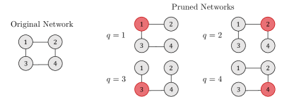
The proof will be accompanied by an example network topology, given in Figure 3
At a fixed point \macc@depth Δ \frozen@everymath \macc@group \macc@set@skewchar \macc@nested@a 111 X = X i + 1 = X i \macc@depth Δ \frozen@everymath \macc@group \macc@set@skewchar \macc@nested@a 111 𝑋 superscript 𝑋 𝑖 1 superscript 𝑋 𝑖 \macc@depth\char 1\relax\frozen@everymath{\macc@group}\macc@set@skewchar\macc@nested@a 111{X}=X^{i+1}=X^{i} LABEL:main-app:dasf_conv_2 in [1 ] that at each node q ∈ 𝒦 𝑞 𝒦 q\in\mathcal{K}
\macc@depth Δ \frozen@everymath \macc@group \macc@set@skewchar \macc@nested@a 111 X q T ∇ X q f ( \macc@depth Δ \frozen@everymath \macc@group \macc@set@skewchar \macc@nested@a 111 X ) \macc@depth Δ \frozen@everymath \macc@group \macc@set@skewchar \macc@nested@a 111 superscript subscript 𝑋 𝑞 𝑇 subscript ∇ subscript 𝑋 𝑞 𝑓 \macc@depth Δ \frozen@everymath \macc@group \macc@set@skewchar \macc@nested@a 111 𝑋 \displaystyle\macc@depth\char 1\relax\frozen@everymath{\macc@group}\macc@set@skewchar\macc@nested@a 111{X}_{q}^{T}\nabla_{X_{q}}f(\macc@depth\char 1\relax\frozen@everymath{\macc@group}\macc@set@skewchar\macc@nested@a 111{X}) = − ∑ j ∈ 𝒥 λ j ( q ) \macc@depth Δ \frozen@everymath \macc@group \macc@set@skewchar \macc@nested@a 111 X q T ∇ X q h j ( \macc@depth Δ \frozen@everymath \macc@group \macc@set@skewchar \macc@nested@a 111 X ) , absent subscript 𝑗 𝒥 subscript 𝜆 𝑗 𝑞 \macc@depth Δ \frozen@everymath \macc@group \macc@set@skewchar \macc@nested@a 111 superscript subscript 𝑋 𝑞 𝑇 subscript ∇ subscript 𝑋 𝑞 subscript ℎ 𝑗 \macc@depth Δ \frozen@everymath \macc@group \macc@set@skewchar \macc@nested@a 111 𝑋 \displaystyle=-\sum_{j\in\mathcal{J}}\lambda_{j}(q)\macc@depth\char 1\relax\frozen@everymath{\macc@group}\macc@set@skewchar\macc@nested@a 111{X}_{q}^{T}\nabla_{X_{q}}h_{j}(\macc@depth\char 1\relax\frozen@everymath{\macc@group}\macc@set@skewchar\macc@nested@a 111{X}), (100)
∑ k ∈ ℬ n q \macc@depth Δ \frozen@everymath \macc@group \macc@set@skewchar \macc@nested@a 111 X k T ∇ X k f ( \macc@depth Δ \frozen@everymath \macc@group \macc@set@skewchar \macc@nested@a 111 X ) subscript 𝑘 subscript ℬ 𝑛 𝑞 \macc@depth Δ \frozen@everymath \macc@group \macc@set@skewchar \macc@nested@a 111 superscript subscript 𝑋 𝑘 𝑇 subscript ∇ subscript 𝑋 𝑘 𝑓 \macc@depth Δ \frozen@everymath \macc@group \macc@set@skewchar \macc@nested@a 111 𝑋 \displaystyle\sum_{k\in\mathcal{B}_{nq}}\macc@depth\char 1\relax\frozen@everymath{\macc@group}\macc@set@skewchar\macc@nested@a 111{X}_{k}^{T}\nabla_{X_{k}}f(\macc@depth\char 1\relax\frozen@everymath{\macc@group}\macc@set@skewchar\macc@nested@a 111{X}) = − ∑ j ∈ 𝒥 ∑ k ∈ ℬ n q λ j ( q ) \macc@depth Δ \frozen@everymath \macc@group \macc@set@skewchar \macc@nested@a 111 X k T ∇ X k h j ( \macc@depth Δ \frozen@everymath \macc@group \macc@set@skewchar \macc@nested@a 111 X ) , absent subscript 𝑗 𝒥 subscript 𝑘 subscript ℬ 𝑛 𝑞 subscript 𝜆 𝑗 𝑞 \macc@depth Δ \frozen@everymath \macc@group \macc@set@skewchar \macc@nested@a 111 superscript subscript 𝑋 𝑘 𝑇 subscript ∇ subscript 𝑋 𝑘 subscript ℎ 𝑗 \macc@depth Δ \frozen@everymath \macc@group \macc@set@skewchar \macc@nested@a 111 𝑋 \displaystyle=-\sum_{j\in\mathcal{J}}\sum_{k\in\mathcal{B}_{nq}}\lambda_{j}(q)\macc@depth\char 1\relax\frozen@everymath{\macc@group}\macc@set@skewchar\macc@nested@a 111{X}_{k}^{T}\nabla_{X_{k}}h_{j}(\macc@depth\char 1\relax\frozen@everymath{\macc@group}\macc@set@skewchar\macc@nested@a 111{X}), (101)
∀ n ∈ 𝒩 q for-all 𝑛 subscript 𝒩 𝑞 \forall n\in\mathcal{N}_{q}
∑ j ∈ 𝒥 ∑ k ∈ ℬ n q λ j ( k ) \macc@depth Δ \frozen@everymath \macc@group \macc@set@skewchar \macc@nested@a 111 X k T ∇ X k h j ( \macc@depth Δ \frozen@everymath \macc@group \macc@set@skewchar \macc@nested@a 111 X ) subscript 𝑗 𝒥 subscript 𝑘 subscript ℬ 𝑛 𝑞 subscript 𝜆 𝑗 𝑘 \macc@depth Δ \frozen@everymath \macc@group \macc@set@skewchar \macc@nested@a 111 superscript subscript 𝑋 𝑘 𝑇 subscript ∇ subscript 𝑋 𝑘 subscript ℎ 𝑗 \macc@depth Δ \frozen@everymath \macc@group \macc@set@skewchar \macc@nested@a 111 𝑋 \displaystyle\sum_{j\in\mathcal{J}}\sum_{k\in\mathcal{B}_{nq}}\lambda_{j}(k)\macc@depth\char 1\relax\frozen@everymath{\macc@group}\macc@set@skewchar\macc@nested@a 111{X}_{k}^{T}\nabla_{X_{k}}h_{j}(\macc@depth\char 1\relax\frozen@everymath{\macc@group}\macc@set@skewchar\macc@nested@a 111{X}) (102)
= \displaystyle= ∑ j ∈ 𝒥 ∑ k ∈ ℬ n q λ j ( q ) \macc@depth Δ \frozen@everymath \macc@group \macc@set@skewchar \macc@nested@a 111 X k T ∇ X k h j ( \macc@depth Δ \frozen@everymath \macc@group \macc@set@skewchar \macc@nested@a 111 X ) , ∀ n ∈ 𝒩 q . subscript 𝑗 𝒥 subscript 𝑘 subscript ℬ 𝑛 𝑞 subscript 𝜆 𝑗 𝑞 \macc@depth Δ \frozen@everymath \macc@group \macc@set@skewchar \macc@nested@a 111 superscript subscript 𝑋 𝑘 𝑇 subscript ∇ subscript 𝑋 𝑘 subscript ℎ 𝑗 \macc@depth Δ \frozen@everymath \macc@group \macc@set@skewchar \macc@nested@a 111 𝑋 for-all 𝑛
subscript 𝒩 𝑞 \displaystyle\sum_{j\in\mathcal{J}}\sum_{k\in\mathcal{B}_{nq}}\lambda_{j}(q)\macc@depth\char 1\relax\frozen@everymath{\macc@group}\macc@set@skewchar\macc@nested@a 111{X}_{k}^{T}\nabla_{X_{k}}h_{j}(\macc@depth\char 1\relax\frozen@everymath{\macc@group}\macc@set@skewchar\macc@nested@a 111{X}),\;\forall n\in\mathcal{N}_{q}.
For clarity, we vectorize the the matrices \macc@depth Δ \frozen@everymath \macc@group \macc@set@skewchar \macc@nested@a 111 X k T ∇ X k h j ( \macc@depth Δ \frozen@everymath \macc@group \macc@set@skewchar \macc@nested@a 111 X ) \macc@depth Δ \frozen@everymath \macc@group \macc@set@skewchar \macc@nested@a 111 superscript subscript 𝑋 𝑘 𝑇 subscript ∇ subscript 𝑋 𝑘 subscript ℎ 𝑗 \macc@depth Δ \frozen@everymath \macc@group \macc@set@skewchar \macc@nested@a 111 𝑋 \macc@depth\char 1\relax\frozen@everymath{\macc@group}\macc@set@skewchar\macc@nested@a 111{X}_{k}^{T}\nabla_{X_{k}}h_{j}(\macc@depth\char 1\relax\frozen@everymath{\macc@group}\macc@set@skewchar\macc@nested@a 111{X}) 𝐡 j , k = vec ( \macc@depth Δ \frozen@everymath \macc@group \macc@set@skewchar \macc@nested@a 111 X k T ∇ X k h j ( \macc@depth Δ \frozen@everymath \macc@group \macc@set@skewchar \macc@nested@a 111 X ) ) ∈ ℝ Q 2 subscript 𝐡 𝑗 𝑘
vec \macc@depth Δ \frozen@everymath \macc@group \macc@set@skewchar \macc@nested@a 111 superscript subscript 𝑋 𝑘 𝑇 subscript ∇ subscript 𝑋 𝑘 subscript ℎ 𝑗 \macc@depth Δ \frozen@everymath \macc@group \macc@set@skewchar \macc@nested@a 111 𝑋 superscript ℝ superscript 𝑄 2 \mathbf{h}_{j,k}=\text{vec}\left(\macc@depth\char 1\relax\frozen@everymath{\macc@group}\macc@set@skewchar\macc@nested@a 111{X}_{k}^{T}\nabla_{X_{k}}h_{j}(\macc@depth\char 1\relax\frozen@everymath{\macc@group}\macc@set@skewchar\macc@nested@a 111{X})\right)\in\mathbb{R}^{Q^{2}} H k = [ 𝐡 1 , k , … , 𝐡 J , k ] ∈ ℝ Q 2 × J subscript 𝐻 𝑘 subscript 𝐡 1 𝑘
… subscript 𝐡 𝐽 𝑘
superscript ℝ superscript 𝑄 2 𝐽 H_{k}=[\mathbf{h}_{1,k},\dots,\mathbf{h}_{J,k}]\in\mathbb{R}^{Q^{2}\times J} ∀ k ∈ 𝒦 for-all 𝑘 𝒦 \forall k\in\mathcal{K} { D j , q } j subscript subscript 𝐷 𝑗 𝑞
𝑗 \{D_{j,q}\}_{j} q 𝑞 q
𝐃 𝐪 = [ H q ∑ k ∈ ℬ n 1 q H k ⋮ ∑ k ∈ ℬ n | 𝒩 q | q H k ] subscript 𝐃 𝐪 matrix subscript 𝐻 𝑞 subscript 𝑘 subscript ℬ subscript 𝑛 1 𝑞 subscript 𝐻 𝑘 ⋮ subscript 𝑘 subscript ℬ subscript 𝑛 subscript 𝒩 𝑞 𝑞 subscript 𝐻 𝑘 \mathbf{D_{q}}=\begin{bmatrix}H_{q}\\
\sum_{k\in\mathcal{B}_{n_{1}q}}H_{k}\\
\vdots\\
\sum_{k\in\mathcal{B}_{n_{|\mathcal{N}_{q}|}q}}H_{k}\end{bmatrix} (103)
being full rank, i.e., rank ( 𝐃 𝐪 ) = J rank subscript 𝐃 𝐪 𝐽 \text{rank}(\mathbf{D_{q}})=J 102
∑ k ∈ ℬ n q H k 𝝀 ( k ) = ( ∑ k ∈ ℬ n q H k ) 𝝀 ( q ) , ∀ n ∈ 𝒩 q , formulae-sequence subscript 𝑘 subscript ℬ 𝑛 𝑞 subscript 𝐻 𝑘 𝝀 𝑘 subscript 𝑘 subscript ℬ 𝑛 𝑞 subscript 𝐻 𝑘 𝝀 𝑞 for-all 𝑛 subscript 𝒩 𝑞 \sum_{k\in\mathcal{B}_{nq}}H_{k}\bm{\lambda}(k)=\left(\sum_{k\in\mathcal{B}_{nq}}H_{k}\right)\bm{\lambda}(q),\;\forall n\in\mathcal{N}_{q}, (104)
where 𝝀 ( k ) = [ λ 1 ( k ) , … , λ J ( k ) ] T 𝝀 𝑘 superscript subscript 𝜆 1 𝑘 … subscript 𝜆 𝐽 𝑘
𝑇 \bm{\lambda}(k)=[\lambda_{1}(k),\dots,\lambda_{J}(k)]^{T} 3 q = 1 𝑞 1 q=1
H 2 𝝀 ( 2 ) = H 2 𝝀 ( 1 ) , subscript 𝐻 2 𝝀 2 subscript 𝐻 2 𝝀 1 \displaystyle H_{2}\bm{\lambda}(2)=H_{2}\bm{\lambda}(1), (105)
H 3 𝝀 ( 3 ) + H 4 𝝀 ( 4 ) = ( H 3 + H 4 ) 𝝀 ( 1 ) . subscript 𝐻 3 𝝀 3 subscript 𝐻 4 𝝀 4 subscript 𝐻 3 subscript 𝐻 4 𝝀 1 \displaystyle H_{3}\bm{\lambda}(3)+H_{4}\bm{\lambda}(4)=(H_{3}+H_{4})\bm{\lambda}(1). (106)
Figure 3 : The example 4 − limit-from 4 4-
Equation (104
𝐇 n q ⋅ 𝝀 𝒦 = 0 , ⋅ subscript 𝐇 𝑛 𝑞 subscript 𝝀 𝒦 0 \mathbf{H}_{nq}\cdot\bm{\lambda}_{\mathcal{K}}=0, (107)
with 𝐇 n q subscript 𝐇 𝑛 𝑞 \mathbf{H}_{nq} l ∈ 𝒦 𝑙 𝒦 l\in\mathcal{K}
𝐇 n q ( l ) = { − ∑ k ∈ ℬ n q H k if l = q H l if l ∈ ℬ n q 0 otherwise. subscript 𝐇 𝑛 𝑞 𝑙 cases subscript 𝑘 subscript ℬ 𝑛 𝑞 subscript 𝐻 𝑘 if l = q subscript 𝐻 𝑙 if l ∈ ℬ n q 0 otherwise. \mathbf{H}_{nq}(l)=\begin{cases}-\sum_{k\in\mathcal{B}_{nq}}H_{k}&\text{if $l=q$}\\
H_{l}&\text{if $l\in\mathcal{B}_{nq}$}\\
0&\text{otherwise.}\end{cases} (108)
We can then stack vertically every 𝐇 n q subscript 𝐇 𝑛 𝑞 \mathbf{H}_{nq} n ∈ 𝒩 q 𝑛 subscript 𝒩 𝑞 n\in\mathcal{N}_{q} q 𝑞 q q 𝑞 q
𝐇 ⋅ 𝝀 𝒦 = 0 . ⋅ 𝐇 subscript 𝝀 𝒦 0 \mathbf{H}\cdot\bm{\lambda}_{\mathcal{K}}=0. (109)
In the example network of Figure 3 110
Note that 𝐇 𝐇 \mathbf{H} Q 2 ∑ k ∈ 𝒦 | 𝒩 k | × K J superscript 𝑄 2 subscript 𝑘 𝒦 subscript 𝒩 𝑘 𝐾 𝐽 Q^{2}\sum_{k\in\mathcal{K}}|\mathcal{N}_{k}|\times KJ ∀ q ∈ 𝒦 for-all 𝑞 𝒦 \forall q\in\mathcal{K} n ∈ 𝒩 q 𝑛 subscript 𝒩 𝑞 n\in\mathcal{N}_{q}
∑ k ∈ 𝒦 \ { l } 𝐇 n q ( k ) = − 𝐇 n q ( l ) subscript 𝑘 \ 𝒦 𝑙 subscript 𝐇 𝑛 𝑞 𝑘 subscript 𝐇 𝑛 𝑞 𝑙 \sum_{k\in\mathcal{K}\backslash\{l\}}\mathbf{H}_{nq}(k)=-\mathbf{H}_{nq}(l) (111)
∀ l ∈ 𝒦 for-all 𝑙 𝒦 \forall l\in\mathcal{K} 𝝀 𝒦 ∈ ℝ K J subscript 𝝀 𝒦 superscript ℝ 𝐾 𝐽 \bm{\lambda}_{\mathcal{K}}\in\mathbb{R}^{KJ} 𝝀 ( 1 ) = ⋯ = 𝝀 ( K ) 𝝀 1 ⋯ 𝝀 𝐾 \bm{\lambda}(1)=\dots=\bm{\lambda}(K) 109
ℰ = { [ 𝐞 1 ⋮ 𝐞 1 ] , [ 𝐞 2 ⋮ 𝐞 2 ] , … [ 𝐞 J ⋮ 𝐞 J ] } ⊂ ℝ K J , ℰ matrix subscript 𝐞 1 ⋮ subscript 𝐞 1 matrix subscript 𝐞 2 ⋮ subscript 𝐞 2 … matrix subscript 𝐞 𝐽 ⋮ subscript 𝐞 𝐽 superscript ℝ 𝐾 𝐽 \mathcal{E}=\left\{\begin{bmatrix}\mathbf{e}_{1}\\
\vdots\\
\mathbf{e}_{1}\end{bmatrix},\begin{bmatrix}\mathbf{e}_{2}\\
\vdots\\
\mathbf{e}_{2}\end{bmatrix},\dots\begin{bmatrix}\mathbf{e}_{J}\\
\vdots\\
\mathbf{e}_{J}\end{bmatrix}\right\}\subset\mathbb{R}^{KJ}, (112)
where 𝐞 k subscript 𝐞 𝑘 \mathbf{e}_{k} ℝ J superscript ℝ 𝐽 \mathbb{R}^{J} ℰ ℰ \mathcal{E} J − limit-from 𝐽 J-
rank ( 𝐇 ) ≤ K J − J . rank 𝐇 𝐾 𝐽 𝐽 \text{rank}(\mathbf{H})\leq KJ-J. (113)
To show that the solution of (109 𝝀 ( 1 ) = ⋯ = 𝝀 ( K ) 𝝀 1 ⋯ 𝝀 𝐾 \bm{\lambda}(1)=\dots=\bm{\lambda}(K) span ( ℰ ) span ℰ \text{span}(\mathcal{E}) rank ( 𝐇 ) = K J − J rank 𝐇 𝐾 𝐽 𝐽 \text{rank}(\mathbf{H})=KJ-J LABEL:main-lem:rank_H from [1 ] , repeated below and followed by a proof. By the dimensions of 𝐇 𝐇 \mathbf{H} Q 2 ∑ k ∈ 𝒦 | 𝒩 k | ≥ K J − J superscript 𝑄 2 subscript 𝑘 𝒦 subscript 𝒩 𝑘 𝐾 𝐽 𝐽 Q^{2}\sum_{k\in\mathcal{K}}|\mathcal{N}_{k}|\geq KJ-J J ≤ Q 2 K − 1 ∑ k ∈ 𝒦 | 𝒩 k | 𝐽 superscript 𝑄 2 𝐾 1 subscript 𝑘 𝒦 subscript 𝒩 𝑘 J\leq\frac{Q^{2}}{K-1}\sum_{k\in\mathcal{K}}|\mathcal{N}_{k}|
Lemma LABEL:main-lem:rank_H .
If Condition LABEL:main-cond:lin_indep_2 holds, then rank ( 𝐇 ) = K J − J rank 𝐇 𝐾 𝐽 𝐽 \text{rank}(\mathbf{H})=KJ-J
Proof.
Let us take the bottom part of the matrix 𝐇 𝐇 \mathbf{H} K 𝐾 K 𝐇 n K subscript 𝐇 𝑛 𝐾 \mathbf{H}_{nK} n ∈ 𝒩 K 𝑛 subscript 𝒩 𝐾 n\in\mathcal{N}_{K} 108
𝐇 Σ K ( l ) = { − ∑ k ∈ 𝒦 \ { K } H k if l = K H l if l ≠ K . subscript 𝐇 Σ 𝐾 𝑙 cases subscript 𝑘 \ 𝒦 𝐾 subscript 𝐻 𝑘 if l = K subscript 𝐻 𝑙 if l ≠ K \mathbf{H}_{\Sigma K}(l)=\begin{cases}-\sum_{k\in\mathcal{K}\backslash\{K\}}H_{k}&\text{if $l=K$}\\
H_{l}&\text{if $l\neq K$}.\end{cases} (114)
In the example network, we have K = 4 𝐾 4 K=4
𝐇 Σ 4 = [ H 1 H 2 H 3 − H 1 − H 2 − H 3 ] . subscript 𝐇 Σ 4 delimited-[] subscript 𝐻 1 missing-subexpression subscript 𝐻 2 missing-subexpression subscript 𝐻 3 missing-subexpression subscript 𝐻 1 subscript 𝐻 2 subscript 𝐻 3 missing-subexpression \mathbf{H}_{\Sigma 4}=\left[\begin{array}[]{@{}*{8}{c}@{}}H_{1}&\vline&H_{2}&\vline&H_{3}&\vline&-H_{1}-H_{2}-H_{3}\end{array}\right]. (115)
We then insert vertically the matrices 𝐇 Σ K subscript 𝐇 Σ 𝐾 \mathbf{H}_{\Sigma K} 𝐇 n | 𝒩 q | q subscript 𝐇 subscript 𝑛 subscript 𝒩 𝑞 𝑞 \mathbf{H}_{n_{|\mathcal{N}_{q}|}q} q ≠ K 𝑞 𝐾 q\neq K 𝐇 𝐇 \mathbf{H} 𝐇 𝐇 \mathbf{H} [ 𝐇 n 1 K T , … , 𝐇 n | 𝒩 K | K T ] T superscript subscript superscript 𝐇 𝑇 subscript 𝑛 1 𝐾 … subscript superscript 𝐇 𝑇 subscript 𝑛 subscript 𝒩 𝐾 𝐾
𝑇 [\mathbf{H}^{T}_{n_{1}K},\dots,\mathbf{H}^{T}_{n_{|\mathcal{N}_{K}|}K}]^{T} K 𝐾 K 𝐇 ~ ~ 𝐇 \widetilde{\mathbf{H}} 3 116
rank ( 𝐇 ) ≥ rank ( 𝐇 ~ ) rank 𝐇 rank ~ 𝐇 \text{rank}(\mathbf{H})\geq\text{rank}(\widetilde{\mathbf{H}}) (117)
since the removal of rows can only reduce the rank.
We will first look at the rank of 𝐇 ~ ~ 𝐇 \widetilde{\mathbf{H}} 𝐇 𝐇 \mathbf{H} 116 𝐇 ~ ~ 𝐇 \widetilde{\mathbf{H}} K 𝐾 K 𝐇 ~ ~ 𝐇 \widetilde{\mathbf{H}} the block-column at position k ∈ 𝒦 𝑘 𝒦 k\in\mathcal{K} [ 𝐇 n 1 q T , … , 𝐇 n | 𝒩 q | q T , 𝐇 Σ K ] T superscript subscript superscript 𝐇 𝑇 subscript 𝑛 1 𝑞 … subscript superscript 𝐇 𝑇 subscript 𝑛 subscript 𝒩 𝑞 𝑞 subscript 𝐇 Σ 𝐾
𝑇 [\mathbf{H}^{T}_{n_{1}q},\dots,\mathbf{H}^{T}_{n_{|\mathcal{N}_{q}|q}},\mathbf{H}_{\Sigma K}]^{T} q ≠ K 𝑞 𝐾 q\neq K the submatrix corresponding to node q 𝑞 q 116 3 3 3 2 2 2 [ H 3 T , 0 , H 3 T ] T superscript superscript subscript 𝐻 3 𝑇 0 superscript subscript 𝐻 3 𝑇
𝑇 [H_{3}^{T},0,H_{3}^{T}]^{T}
For each q ≠ K 𝑞 𝐾 q\neq K 𝐇 n q subscript 𝐇 𝑛 𝑞 \mathbf{H}_{nq} n ∈ 𝒩 q 𝑛 subscript 𝒩 𝑞 n\in\mathcal{N}_{q} 𝐇 Σ K subscript 𝐇 Σ 𝐾 \mathbf{H}_{\Sigma K} q 𝑞 q [ 0 | … | 0 | ∑ k ∈ 𝒦 H k | 0 | … | 0 | − ∑ k ∈ 𝒦 H k ] delimited-[] conditional 0 … 0 subscript 𝑘 𝒦 subscript 𝐻 𝑘 0 … 0 subscript 𝑘 𝒦 subscript 𝐻 𝑘 [0|\dots|0|\sum_{k\in\mathcal{K}}H_{k}|0|\dots|0|-\sum_{k\in\mathcal{K}}H_{k}] q ≠ K 𝑞 𝐾 q\neq K
An important observation is that, for each q ≠ K 𝑞 𝐾 q\neq K q 𝑞 q q 𝑞 q 𝐃 𝐪 subscript 𝐃 𝐪 \mathbf{D_{q}} 103 𝐃 𝐪 subscript 𝐃 𝐪 \mathbf{D_{q}} rank ( 𝐃 𝐪 ) = J rank subscript 𝐃 𝐪 𝐽 \text{rank}(\mathbf{D_{q}})=J LABEL:main-cond:lin_indep_2 , we can apply the necessary EROs to obtain the following reduced echelon form for the submatrix corresponding to node q = 1 𝑞 1 q=1
[ I J ∗ ⋯ ∗ ∗ 0 ] . delimited-[] subscript 𝐼 𝐽 missing-subexpression missing-subexpression ⋯ missing-subexpression missing-subexpression missing-subexpression 0 missing-subexpression missing-subexpression missing-subexpression missing-subexpression missing-subexpression \left[\begin{array}[]{@{}*{10}{c}@{}}I_{J}&\vline&\hbox{\multirowsetup$*$}&\vline&\hbox{\multirowsetup$\cdots$}&\vline&\hbox{\multirowsetup$*$}&\vline&\hbox{\multirowsetup$*$}&\\
0&\vline&&\vline&&\vline&&\vline&&\end{array}\right]. (119)
We can use the J 𝐽 J J 𝐽 J 119 q ≠ 1 𝑞 1 q\neq 1
[ I J ∗ ⋯ ∗ ∗ 0 0 ℛ 𝐃 𝟐 ⋯ ⋮ ⋮ ⋱ ⋮ ⋮ 0 ∗ ⋯ ] , delimited-[] subscript 𝐼 𝐽 missing-subexpression missing-subexpression ⋯ missing-subexpression missing-subexpression missing-subexpression 0 missing-subexpression missing-subexpression missing-subexpression missing-subexpression missing-subexpression missing-subexpression missing-subexpression missing-subexpression missing-subexpression missing-subexpression missing-subexpression 0 missing-subexpression ℛ subscript 𝐃 2 missing-subexpression ⋯ missing-subexpression missing-subexpression missing-subexpression missing-subexpression missing-subexpression missing-subexpression missing-subexpression missing-subexpression missing-subexpression missing-subexpression missing-subexpression missing-subexpression missing-subexpression ⋮ missing-subexpression ⋮ missing-subexpression ⋱ missing-subexpression ⋮ missing-subexpression ⋮ missing-subexpression missing-subexpression missing-subexpression missing-subexpression missing-subexpression missing-subexpression missing-subexpression missing-subexpression missing-subexpression missing-subexpression missing-subexpression 0 missing-subexpression missing-subexpression ⋯ missing-subexpression ℛ subscript 𝐃 𝐊 1 missing-subexpression missing-subexpression \left[\begin{array}[]{@{}*{10}{c}@{}}I_{J}&\vline&\hbox{\multirowsetup$*$}&\vline&\hbox{\multirowsetup$\cdots$}&\vline&\hbox{\multirowsetup$*$}&\vline&\hbox{\multirowsetup$*$}&\\
0&\vline&&\vline&&\vline&&\vline&&\\
\hline\cr\hbox{\multirowsetup$0$}&\vline&\hbox{\multirowsetup$\mathcal{R}\mathbf{D_{2}}$}&\vline&\hbox{\multirowsetup$\cdots$}&\vline&\hbox{\multirowsetup$*$}&\vline&\hbox{\multirowsetup$*$}&\\
&\vline&&\vline&&\vline&&\vline&&\\
\hline\cr\hbox{\multirowsetup$\vdots$}&\vline&\hbox{\multirowsetup$\vdots$}&\vline&\hbox{\multirowsetup$\ddots$}&\vline&\hbox{\multirowsetup$\vdots$}&\vline&\hbox{\multirowsetup$\vdots$}&\\
&\vline&&\vline&&\vline&&\vline&&\\
\hline\cr\hbox{\multirowsetup$0$}&\vline&\hbox{\multirowsetup$*$}&\vline&\hbox{\multirowsetup$\cdots$}&\vline&\hbox{\multirowsetup$\mathcal{R}\mathbf{D_{K-1}}$}&\vline&\hbox{\multirowsetup$*$}&\\
&\vline&&\vline&&\vline&&\vline&&\end{array}\right], (120)
where ℛ 𝐃 𝐤 ℛ subscript 𝐃 𝐤 \mathcal{R}\mathbf{D_{k}} 𝐃 𝐤 subscript 𝐃 𝐤 \mathbf{D_{k}} 120 k ∉ { 1 , K } 𝑘 1 𝐾 k\notin\{1,K\} k 𝑘 k 𝐃 𝐤 subscript 𝐃 𝐤 \mathbf{D_{k}} H k subscript 𝐻 𝑘 H_{k} 118 J 𝐽 J q = 1 𝑞 1 q=1 k 𝑘 k k 𝑘 k 𝐃 𝐤 subscript 𝐃 𝐤 \mathbf{D_{k}} ℛ 𝐃 𝟐 ℛ subscript 𝐃 2 \mathcal{R}\mathbf{D_{2}} J 𝐽 J J 𝐽 J 2 ≤ q ≤ K − 1 2 𝑞 𝐾 1 2\leq q\leq K-1
[ I J ∗ ⋯ ∗ ∗ 0 0 I J ⋯ 0 ⋮ ⋮ ⋱ ⋮ ⋮ 0 0 ⋯ 0 ] . delimited-[] subscript 𝐼 𝐽 missing-subexpression missing-subexpression ⋯ missing-subexpression missing-subexpression missing-subexpression 0 missing-subexpression missing-subexpression missing-subexpression missing-subexpression missing-subexpression missing-subexpression missing-subexpression missing-subexpression missing-subexpression missing-subexpression missing-subexpression 0 missing-subexpression subscript 𝐼 𝐽 missing-subexpression ⋯ missing-subexpression missing-subexpression missing-subexpression missing-subexpression 0 missing-subexpression missing-subexpression missing-subexpression missing-subexpression missing-subexpression missing-subexpression missing-subexpression missing-subexpression missing-subexpression missing-subexpression ⋮ missing-subexpression ⋮ missing-subexpression ⋱ missing-subexpression ⋮ missing-subexpression ⋮ missing-subexpression missing-subexpression missing-subexpression missing-subexpression missing-subexpression missing-subexpression missing-subexpression missing-subexpression missing-subexpression missing-subexpression missing-subexpression 0 missing-subexpression 0 missing-subexpression ⋯ missing-subexpression subscript 𝐼 𝐽 missing-subexpression missing-subexpression missing-subexpression missing-subexpression missing-subexpression 0 missing-subexpression missing-subexpression \left[\begin{array}[]{@{}*{10}{c}@{}}I_{J}&\vline&\hbox{\multirowsetup$*$}&\vline&\hbox{\multirowsetup$\cdots$}&\vline&\hbox{\multirowsetup$*$}&\vline&\hbox{\multirowsetup$*$}&\\
0&\vline&&\vline&&\vline&&\vline&&\\
\hline\cr\hbox{\multirowsetup$0$}&\vline&I_{J}&\vline&\hbox{\multirowsetup$\cdots$}&\vline&\hbox{\multirowsetup$*$}&\vline&\hbox{\multirowsetup$*$}&\\
&\vline&0&\vline&&\vline&&\vline&&\\
\hline\cr\hbox{\multirowsetup$\vdots$}&\vline&\hbox{\multirowsetup$\vdots$}&\vline&\hbox{\multirowsetup$\ddots$}&\vline&\hbox{\multirowsetup$\vdots$}&\vline&\hbox{\multirowsetup$\vdots$}&\\
&\vline&&\vline&&\vline&&\vline&&\\
\hline\cr\hbox{\multirowsetup$0$}&\vline&\hbox{\multirowsetup$0$}&\vline&\hbox{\multirowsetup$\cdots$}&\vline&I_{J}&\vline&\hbox{\multirowsetup$*$}&\\
&\vline&&\vline&&\vline&0&\vline&&\end{array}\right]. (121)
Since there are at least K − 1 𝐾 1 K-1 J 𝐽 J rank ( 𝐇 ~ ) ≥ K J − J rank ~ 𝐇 𝐾 𝐽 𝐽 \text{rank}(\widetilde{\mathbf{H}})\geq KJ-J 117 rank ( 𝐇 ) ≥ rank ( 𝐇 ~ ) rank 𝐇 rank ~ 𝐇 \text{rank}(\mathbf{H})\geq\text{rank}(\widetilde{\mathbf{H}}) rank ( 𝐇 ) ≥ K J − J rank 𝐇 𝐾 𝐽 𝐽 \text{rank}(\mathbf{H})\geq KJ-J 113 rank ( 𝐇 ) ≤ K J − J rank 𝐇 𝐾 𝐽 𝐽 \text{rank}(\mathbf{H})\leq KJ-J rank ( 𝐇 ) = K J − J rank 𝐇 𝐾 𝐽 𝐽 \text{rank}(\mathbf{H})=KJ-J
References
[1]
C. A. Musluoglu, C. Hovine, and A. Bertrand, “A unified algorithmic framework for distributed adaptive signal and feature fusion problems — Part II: Convergence properties,” 2022.