Out-of-distribution Detection via Frequency-regularized Generative Models

Abstract

Modern deep generative models can assign high likelihood to inputs drawn from outside the training distribution, posing threats to models in open-world deployments. While much research attention has been placed on defining new test-time measures of OOD uncertainty, these methods do not fundamentally change how deep generative models are regularized and optimized in training. In particular, generative models are shown to overly rely on the background information to estimate the likelihood. To address the issue, we propose a novel frequency-regularized learning (FRL) framework for OOD detection, which incorporates high-frequency information into training and guides the model to focus on semantically relevant features. FRL effectively improves performance on a wide range of generative architectures, including variational auto-encoder, GLOW, and PixelCNN++. On a new large-scale evaluation task, FRL achieves the state-of-the-art performance, outperforming a strong baseline Likelihood Regret by 10.7% (AUROC) while achieving 147$\times$ faster inference speed. Extensive ablations show that FRL improves the OOD detection performance while preserving the image generation quality. Code is available at https://github.com/mu-cai/FRL.

1 Introduction

Modern deep generative models have achieved unprecedented success in known contexts for which they are trained, yet they do not necessarily know what they don’t know. In particular, Nalisnick et al. [32] showed that generative models can produce abnormally high likelihood estimation for out-of-distribution (OOD) data—samples with semantics outside the training data distribution. Ideally, a model trained on MNIST should not produce a high likelihood score for an animal image, because the semantic is clearly different from hand-written digits.

This intriguing yet bewildering observation has triggered a plethora of literature to address the problem of OOD detection in generative modeling. Much of the prior work focused on defining more suitable test-time measures of OOD uncertainty, such as Likelihood Ratio [36], Input Complexity [39], and Likelihood Regret [48]. Despite the improved performance, these methods do not fundamentally change how deep generative models are trained and optimized. Arguably, continued research progress in OOD detection requires the improved design of learning methods, in addition to the inference-time statistical tests. This paper bridges this critical gap.

In this paper, we propose a novel Frequency-Regularized Learning framework for OOD detection (dubbed FRL). Our work is motivated by observations in Ren et al. [36], which suggested that generative models’ reliance on the background information undesirably leads to a high likelihood for OOD samples. Indeed, several recent studies [55, 31, 21] showed that current generative models overfit to the training data, particularly background pixels. To alleviate the issue, our key idea is to guide the model to pay more attention to the high-frequency information, which represents object contours and semantic details rather than the low-frequency image background. Shown in Figure 2, though OOD and in-distribution data have similar backgrounds, their high-frequency information represents semantic feature differences well. Our framework is grounded in classic signal processing [40, 3, 13], which demonstrated the efficacy of high-frequency components for capturing semantic content. In particular, FRL adds the high-frequency component as an additional channel to the input image, which regularizes deep generative models to have less reliance on background information and thus improves test-time OOD detection.

FRL provides a general plug-and-play mechanism, which is applicable to common generative models, including Variational Auto-Encoder (VAE) [20, 14], GLOW [19], and PixelCNN++ [35, 38]. Importantly, our method incurs minimal changes to the existing training architecture, and only requires modifying the number of the input channel. FRL is straightforward and relatively simple to implement in practice. During the test time, we concatenate the original image with the high-frequency component, and estimate the OOD score on the concatenated input.

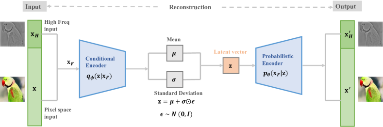
Figure 1: Overview of the proposed frequency-regularized learning framework (FRL) for OOD detection. We exemplify using the VAE architecture. The key idea is to extract the high-frequency information from the original image, and use that for regularizing the generative models. High frequency information captures the outline of objects as opposed to background.

We extensively evaluate our approach on various generative modeling architectures and datasets, where FRL establishes state-of-the-art performance. On flow-based model GLOW, FRL improves the performance on CIFAR-10 by 7.5$\%$ (AUROC), compared to the best baseline Input Complexity [39]. While prior literature has primarily evaluated performance on simple datasets such as CIFAR-10 and Fashion-MNIST, we further extend our evaluation to a large-scale setting and test the limit of our approach. On CelebA dataset with higher resolution, FRL outperforms a competitive method Likelihood Regret (LR) [48] by 10.7% in AUROC while achieving 147$\times$ faster inference speed on VAE. Unlike LR, FRL alleviates the need for online optimization during inference time, a major bottleneck that prevents LR from performing real-time OOD detection. Our key contributions and results are summarized as follows:

• We propose a new frequency-regularized OOD detection framework FRL, which regularizes the training of deep generative models by emphasizing high-frequency information. FRL effectively improves performance on common generative modeling methods including VAE, GLOW, and PixelCNN++.

• We extensively evaluate FRL on common benchmarks, along with a new large-scale evaluation task with high-resolution images. FRL achieves the state-of-the-art performance, outperforming a strong baseline Likelihood Regret [48] by 10.7% (AUROC) while achieving 147$\times$ faster inference speed on CelebA. To the best of our knowledge, this is the first work that demonstrates the efficacy of generative-based OOD detection on datasets beyond the CIFAR benchmark.

• We conduct extensive ablations to improve the understanding of the efficacy of our method, highlighting the importance of high-frequency. We show that FRL improves the OOD detection performance while preserving the image generation quality.

2 Preliminaries

We consider the setting of unsupervised learning, where $\mathcal{X}$ denotes the input space. The training set $\mathcal{D}=\{\mathbf{x}_{i}\}_{i=1}^{n}$ is drawn i.i.d. from in-distribution $P_{\mathcal{X}}$. This setting imposes weaker data assumption than discriminative-based OOD detection approaches, which require labeling information.

Out-of-distribution Detection

OOD detection can be viewed as a binary classification problem. At test time, the goal of OOD detection is to decide whether a sample $\mathbf{x}\in\mathcal{X}$ is from in-distribution $P_{\mathcal{X}}$ (ID) or not (OOD). In practice, OOD is often defined by a distribution that simulates unknowns encountered during deployment time, such as samples from an irrelevant semantic (e.g. MNIST vs. cat). The decision can be made via a thresholding mechanism:

$$G_{\lambda}(\mathbf{x})=\begin{cases}\text{ID}&S(\mathbf{x})\leq\lambda\\ \text{OOD}&S(\mathbf{x})>\lambda\end{cases},$$

where samples with lower scores $S(\mathbf{x})$ are classified as ID and vice versa. The threshold $\lambda$ is typically chosen so that a high fraction of ID data (e.g. 95%) is correctly classified. A natural choice of scoring function is to directly estimate the negative log likelihood of the input using generative modeling, which we describe in the next.

3 Method

Our novel frequency-regularized out-of-distribution detection framework is illustrated in Figure 1. In what follows, we first introduce the mechanism of extracting high-frequency information from an image (Section 3.1). Our training object facilitates the preservation of frequency information during the generative modeling process (Section 3.2).

3.1 High Frequency Information

Our work is motivated by prior work by Ren et al. [36], which showed that generative models’ reliance on the background undesirably leads to high likelihood estimation for OOD samples. For example, deep generative models trained on CIFAR-10 can assign a higher likelihood to OOD data from MNIST. To better understand the phenomenon, several recent studies [55, 31, 21] showed that current generative models overfit to the training data, especially the background pixels that are non-essential for determining the image semantics. In contrast, humans can distinguish MNIST images as OOD w.r.t. animal images, based on semantic information.

Motivated by this, the key idea of our framework is to exploit high-frequency information for enhancing generative-based OOD detection. In particular, we alleviate the generative model’s reliance on background information by guiding it to pay more attention to the high-frequency component of images. The high-frequency component is effective in capturing high-level semantic content, as established in classic signal processing literature [40, 3, 13]. Compared to the color space image, high-frequency features can filter out the low-level background information and maintain the key semantic information, shown in Figure 2.

We now introduce details of how to transform the input image $\*\mathbf{x}\in\mathcal{X}$ into the high frequency counterpart $\*\mathbf{x}_{H}$ . The overall procedure is shown in Figure 3. Note that $\*\mathbf{x}_{H}$ has the same spatial dimension as $\*\mathbf{x}$. Specifically, we employ the Gaussian kernel $K_{\sigma}$:

$$K_{\sigma}[m,n] =\frac{1}{2\pi\sigma^{2}}e^{-\frac{1}{2}\left(\frac{m^{2}+n^{2}}{\sigma^{2}}\right)},$$ (1)

where $[m,n]$ denotes the spatial location with respect to the center of an image batch, and $\sigma^{2}$ denotes the variance of the Gaussian function. Following [13], the variance is increased proportionally with the Gaussian kernel size. By conducting convolution on input $\*\mathbf{x}$ using $K_{\sigma}$, we obtain the low frequency (blurred) image $\mathbf{x}_{L}$:

$$\mathbf{x}_{L}[i,j] =\sum_{m=-\frac{k-1}{2}}^{\frac{k-1}{2}}\sum_{n=-\frac{k-1}{2}}^{\frac{k-1}{2}}K_{\sigma}[m,n]\cdot\mathbf{x}[i+m,j+n],$$ (2)

where $k$ denotes the kernel size, and $m,n$ denotes the index of an 2D Gaussian kernel, i.e., $m,n\in[-\frac{k-1}{2},\frac{k-1}{2}]$.

To obtain the high-frequency image $\*\mathbf{x}_{H}$, we first convert color images into grayscale images, and then subtract the low frequency information:

$$\mathbf{x}_{H} ={\texttt{rgb2gray}}(\mathbf{x})-[\texttt{rgb2gray}(\mathbf{x})]_{{L}},$$ (3)

where the rgb2gray function converts the color image to the grayscale image. This operation removes the color and illumination information that is unrelated to the identity and structure. The resulting high-frequency image $\mathbf{x}_{{H}}$ contains the object outlines of the original image. We proceed by introducing the training objective that can leverage the high-frequency information.

3.2 Generative Modeling with High-frequency Information

To enforce the deep generative models to pay more attention to the high frequency, i.e., semantic features, we propose training deep generative models by adding high-frequency component to the input. In other words, we use input $\mathbf{x}_{F}=[\mathbf{x},\mathbf{x}_{H}]$ via channel concatenation (see Figure 1). This way, the deep generative model is incentivized to learn the semantic information, because failure to recover the high-frequency component will incur a reconstruction loss. Our method incurs minimal changes to the architecture by only modifying the number of the input channel. In what follows, we consider three common generative modeling approaches including VAE, GLOW, and PixelCNN++.

3.2.1 Variational Auto-Encoder (VAE)

VAE is a widely known approach for generative modeling [20, 14]. The VAE consists of an encoder $q_{\phi}(\mathbf{z}\mid\mathbf{x}_{F})$ and a decoder $p_{\theta}(\mathbf{x}_{F}\mid\mathbf{z})$ , as illustrated in Figure 1. Given a latent code $\mathbf{z}$ and its prior $p(\mathbf{z})$, the likelihood $p_{\theta}(\mathbf{x}_{F})$ is modeled as:

$$p_{\theta}(\mathbf{x}_{F})=\int_{\mathcal{Z}}p_{\theta}(\mathbf{x}_{F}\mid\mathbf{z})p(\mathbf{z})\mathrm{d}\mathbf{z}.$$ (4)

During training, variational inference is utilized to minimize the evidence lower bound of the log likelihood, which serves as a proxy for the true likelihood [20]:

$$\small\log p_{\theta}(\mathbf{x}_{F}) \geq\mathbb{E}_{q_{\phi}(\mathbf{z}\mid\mathbf{x}_{F})}\left[\log p_{\theta}(\mathbf{x}_{F}\mid\mathbf{z})\right]-D_{\mathrm{KL}}\left[q_{\phi}(\mathbf{z}\mid\mathbf{x}_{F})\|p(\mathbf{z})\right]$$

$$\triangleq\mathcal{L}(\mathbf{x}_{F};\theta,\phi),$$

where $q_{\phi}(\mathbf{z}\mid\mathbf{x}_{F})$ is the variational approximation to the true posterior distribution $p_{\theta}(\mathbf{z}\mid\mathbf{x}_{F})$.

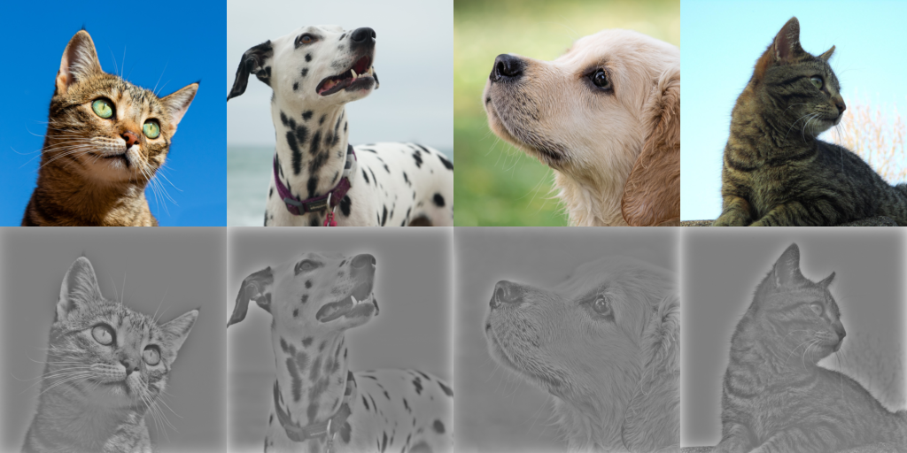
(a) In-distribution

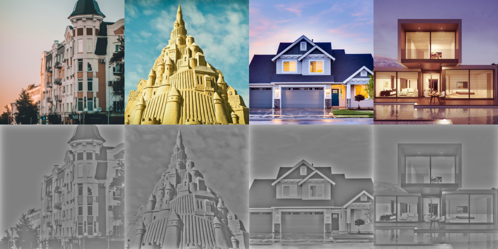
(b) Out-of-distribution

Figure 2: Visualization of the original RGB images and corresponding high-frequency features with similar backgrounds. In-distribution data contains cats and dogs, which are different from out-of-distribution data buildings.

During inference, it is not tractable to directly obtain the log likelihood $\log p_{\theta}(\mathbf{x}_{F})$. Instead, the log likelihood is approximated by the importance weighted lower bound $\mathcal{L}_{K}(\mathbf{x}_{F};\theta,\phi)$:

$$\log p_{\theta}(\mathbf{x}_{F}) \geq\mathbb{E}_{\mathbf{z}^{1},\ldots,\mathbf{z}^{K}\sim q_{\phi}(\mathbf{z}|\mathbf{x}_{F})}\left[\log\frac{1}{K}\sum_{k=1}^{K}\frac{p_{\theta}\left(\mathbf{x}_{F}|\mathbf{z}^{k}\right)p\left(\mathbf{z}^{k}\right)}{q_{\phi}\left(\mathbf{z}^{k}|\mathbf{x}_{F}\right)}\right]$$

$$\triangleq\mathcal{L}_{K}(\mathbf{x}_{F};\theta,\phi),$$

where $\mathbf{z}^{k}$ is a Gaussian sample from the variational posterior $q_{\phi}(\mathbf{z}|\mathbf{x}_{F})$.

3.2.2 GLOW

GLOW [19] adopts the invertible networks [37], without using the encoder-decoder architecture. Specifically, $\mathbf{f}$ is composed of a sequence of transformations: $\mathbf{f}=\mathbf{f}_{1}\circ\mathbf{f}_{2}\circ\cdots\circ\mathbf{f}_{K}$, such that the relationship between $\mathbf{x}_{F}$ and latent code $\mathbf{z}$ can be modeled as:

$$\mathbf{x}_{F}\stackrel{{\scriptstyle\mathbf{f}_{1}}}{{\longleftrightarrow}}\mathbf{h}_{1}\stackrel{{\scriptstyle\mathbf{f}_{2}}}{{\longleftrightarrow}}\mathbf{h}_{2}\cdots\stackrel{{\scriptstyle\mathbf{f}_{K}}}{{\longleftrightarrow}}\mathbf{z},$$ (5)

where $\mathbf{h}_{i}(i=1,\cdots,K-1)$ is the intermediate variable. Such a sequence of invertible transformations is also called a (normalizing) flow. The latent variable $\mathbf{z}$ is generated as a descriptor for the input $\mathbf{x}_{F}$. Then given a datapoint $\mathbf{x}_{F}$, the log probability density function of the model parameterized by $\theta$ can be written as:

$$\log p_{\bm{\theta}}(\mathbf{x}_{F}) =\log p_{\bm{\theta}}(\mathbf{z})+\log|\operatorname{det}(d\mathbf{z}/d\mathbf{x}_{F})|$$ (6)

$$=\log p_{\bm{\theta}}(\mathbf{z})+\sum_{i=1}^{K}\log\left|\operatorname{det}\left(d\mathbf{h}_{i}/d\mathbf{h}_{i-1}\right)\right|.$$

In other words, the log-likelihood $\log p_{\bm{\theta}}(\mathbf{x}_{F})$ is derived using the likelihood of $\mathbf{z}$ and invertible 1$\times$1 convolution modules. The negative log-likelihood (bits per dimension) could be utilized for downstream tasks such as OOD detection.

3.2.3 PixelCNN++

PixelCNN and PixelCNN++ [35, 38] belong to the family of autoregressive models, which sequentially predict the output elements. Given an 2D image $\mathbf{x}_{F}$, PixelCNN++ generates the output image pixel by pixel. Therefore, the joint distribution of pixels over an image $\mathbf{x}_{F}$ can be decomposed into the following product of conditional probabilities:

$$p(\mathbf{x}_{F})=\prod_{i=1}^{n^{2}}p\left(x_{i}\mid x_{1},\ldots,x_{i-1}\right),$$ (7)

where $x_{i}$ is the pixel value in each location. The ordering of the pixel dependencies is in raster scan order: row by row and pixel by pixel within every row. Therefore, each pixel depends on all the pixels above and to the left of it, and not on any of the other pixels.

Figure 3: Illustration on the process of extracting high frequency information. Gaussian blur is used to obtain the low frequency image. The high-frequency component is the difference between the grayscale image and the blurred grayscale image.

3.3 OOD Detection Score

While a straightforward idea is to employ the Negative Log Likelihood score, recent work [39] showed that it is more advantageous to subtract the Input Complexity, resulting in the following function:

$$S(\mathbf{x})=-\log p_{\theta}(\mathbf{x})-L(\mathbf{x}),$$ (8)

where the complexity score $L(\mathbf{x})$ is represented by the code length derived from the data compressors [39]. This score function can also be interpreted from a likelihood-ratio test perspective.

Inspired by this, we employ the frequency-based log-likelihood term to derive a new scoring function $S_{F}(\mathbf{x})$ for OOD detection:

$$S_{F}(\mathbf{x})=-\log p_{\theta}(\mathbf{x}_{F})-L(\mathbf{x}),$$ (9)

where $S_{F}(\mathbf{x})$ captures frequency information for OOD detection. The image compression algorithm to represent the code length $L(\mathbf{x})$ is based on the Portable Network Graphics (PNG) [11] format.

4 Experiments

In this section, we first describe the experimental details (Section 4.1), then we evaluate our approach FRL on various generative modeling architectures and datasets (Section 4.2 & Section 4.3). Further ablation studies are provided in Section 4.4. Extensive experimental results show that FRL not only preserves the image generation capability, but also enhances OOD detection.

4.1 Experimental Details

Common Benchmark

We use CIFAR-10 [22], Fashion-MNIST [46] as the in-distribution datasets. For both datasets, we consider a total of 9 OOD datasets, which are all resized to 32$\times$32. The OOD datasets includes SVHN [33], LSUN [54], MNIST [9], KMNIST [25], Omniglot [23], NotMNIST, Noise, and Constant. In CIFAR-10 evaluation, the OOD dataset also includes Fashion-MNIST, vice versa.

Large-scale Evaluation Datasets

Furthermore, we also evaluate our method on large scale high-resolution dataset CelebA [29]. Following [16], we adopt four high resolution OOD datasets: iNaturalist [41], Places [47], SUN [56], and Textures [6]. All images are resized to $128\times 128$.

Training Details

We provide details for training on each of the architecture: VAE, GLOW and PixelCNN++.

(1) VAE is trained for 100 epochs for CIFAR-10 and Fashion-MNIST, and 110 epochs for CelebA. The Gaussian kernel size is set to be 5, which we provide further ablation in Section 4.4. Following [48], $p_{\theta}(\mathbf{x}\mid\mathbf{z})$ is chosen to be follow the 256-way discrete distribution. In image domain, this distribution corresponds to an 8-bit image on each pixel.

(2) GLOW is trained for 50 epochs with batch size 32 for both CIFAR-10 and Fashion-MNIST. The learning rate is $5\times 10^{-4}$. Following [19], we adopt the invertible $1\times 1$ convolutional (InvConv) layers in GLOW.

(3) PixelCNN++ is trained by 110 epochs with the learning rate $5\times 10^{-4}$. There are overall 160 filters across the model. For the encoding part of the PixelCNN++, the model uses 3 residual blocks consisting of 5 residual layers.

Metric and Hardware

Following the literature [32, 36], we primarily use AUROC as our evaluation metrics for OOD detection. All experiments are conducted on NVIDIA GTX 2080Ti GPUs.

4.2 Evaluation on Common Benchmarks

In this section, we evaluate our approach on the common benchmark, and compare it with competitive generative-based OOD detection methods. We consider the following baselines: Negative Log Likelihood (NLL) [32], Likelihood Ratio (LRatio) [36], Input Complexity (IC) [39], and two variants of Likelihood Regret (LR) [48]: LR(E) which optimizes the encoder, and LR(Z) which optimizes the latent variable. For fair comparison, all the baseline methods are trained and evaluated under consistent setting. Our results reported are averaged across 5 independent runs.

Table 1: AUROC values for OOD detection in GLOW and PixelCNN++ when CIFAR-10 is the in-distribution dataset.

Dataset	GLOW				PixelCNN++
	NLL	LRatio	IC	FRL		NLL	LRatio	IC	FRL
	[32]	[36]	[39]	(ours)		[32]	[36]	[39]	(ours)
SVHN	0.070	0.161	0.883	0.915 $\pm$ 0.001		0.129	0.949	0.737	0.831 $\pm$ 0.002
LSUN	0.890	0.730	0.213	0.114 $\pm$ 0.002		0.852	0.785	0.640	0.569 $\pm$ 0.004
MNIST	0.001	0.003	0.858	0.961 $\pm$ 0.002		0.000	0.092	0.967	0.999 $\pm$ 0.000
FMNIST	0.007	0.007	0.712	0.874 $\pm$ 0.003		0.003	0.494	0.907	0.979 $\pm$ 0.001
KMNIST	0.007	0.008	0.380	0.645 $\pm$ 0.002		0.002	0.341	0.826	0.980 $\pm$ 0.001
Omniglot	0.000	0.001	0.955	0.987 $\pm$ 0.000		0.000	0.951	0.989	1.000 $\pm$ 0.000
NotMNIST	0.006	0.009	0.539	0.720 $\pm$ 0.005		0.003	0.718	0.826	0.979 $\pm$ 0.001
Noise	1.000	0.426	1.000	1.000 $\pm$ 0.000		1.000	1.000	1.000	1.000 $\pm$ 0.000
Constant	0.010	0.053	1.000	1.000 $\pm$ 0.000		0.042	0.428	1.000	1.000 $\pm$ 0.000
Average	0.221	0.155	0.727	0.802$\pm$ 0.001		0.226	0.640	0.877	0.926 $\pm$ 0.001
Num img/$s$ ($\uparrow$)	40.1	20.3	38.6	33.7		20.0	10.7	19.3	16.2
$T_{\text{inference}}(s)$ ($\downarrow$)	0.025	0.049	0.026	0.030		0.050	0.093	0.052	0.062

GLOW

The OOD detection results for CIFAR-10 based on GLOW model are shown in Table 1 (left). Flow-based models use invertible convolutions for estimating the likelihood, thus the parameters of the encoder and decoder are the same. Therefore, Likelihood Regret (LR) is not applicable here. FRL establishes the state-of-the-art performance, outperforming the best baseline Input Complexity (IC) by 7.5% in AUROC. The comparison between our method and IC directly highlights the benefit of using high-frequency information for model regularization as well as inference. Note that Likelihood Ratio (LRatio) does not perform well on the GLOW model. We will contrast our method with LRatio on PixelCNN+ and VAE in the next, where LRatio is more effective.

PixelCNN++

Table 1 (right) shows the OOD detection results using PixelCNN++ [35], where FRL outperforms the baselines. Among all the baselines, LRatio [36] also attempts to mitigate the influence of background information using the Likelihood Ratio statistics. Compared to LRatio, FRL displays an improvement of 28.6% AUROC. This suggests that using frequency information for model regularization can be more effective in mitigating the influence of background. Note that due to the property of sequential prediction in autoregressive models, there are no latent variables and encoders. Hence, Likelihood Regret (LR) is not applicable here.

Table 2: AUROC values for OOD Detection in VAE when CIFAR-10 is the in-distribution dataset.

OOD Dataset	NLL	LRatio	LR(Z)	LR(E)	IC	FRL
	[32]	[36]	[48]	[48]	[39]	(ours)
SVHN	0.081	0.050	0.655	0.959	0.907	0.854 $\pm$ 0.002
LSUN	0.926	0.952	0.456	0.403	0.174	0.449 $\pm$ 0.003
MNIST	0.000	0.902	0.759	0.999	0.984	0.984 $\pm$ 0.000
FMNIST	0.033	0.665	0.732	0.991	0.992	0.993 $\pm$ 0.001
KMNIST	0.011	0.918	0.755	0.999	0.981	0.985 $\pm$ 0.000
Omniglot	0.000	0.937	0.637	0.996	0.988	0.988 $\pm$ 0.001
NotMNIST	0.030	0.492	0.737	0.994	0.988	0.990 $\pm$ 0.000
Noise	1.000	1.000	0.703	0.999	0.167	0.925 $\pm$ 0.002
Constant	0.299	0.353	0.833	0.995	1.000	1.000 $\pm$ 0.000
Average	0.264	0.697	0.696	0.926	0.798	0.906 $\pm$ 0.001
Num img/$s$ ($\uparrow$)	240.8	133.2	1.3	2.6	238.8	169.3
$T_{\text{inference}}(s)$ ($\downarrow$)	0.0042	0.0075	0.7438	0.3783	0.0042	0.0059

VAE

Table 2 shows the OOD detection results on CIFAR-10. We compare with a competitive baseline, Likelihood Regret (LR) [48]. Note that LR employs an online estimation, which incurs excessive inference time in its optimization. The best variant, namely LR(E), can only process 2.6 images per second. In contrast, FRL is computationally efficient (169.3 images per second measured by the inference speed), while achieving comparable performance. Moreover, compared to IC, the failure cases of  LSUN and  Noise are reduced significantly using our method FRL. For example, when using Noise as OOD data, FRL improves the AUROC from 0.167 (IC) to 0.922. This is because the image code length is only the approximation of the complexity score. We also show in appendix that FRL produces a more concentrated score distribution for ID data (green shade), benefiting the OOD detection .

When using Fashion-MNIST as the ID dataset, FRL achieves a strong performance across all OOD datasets, with an average AUROC score of 0.976. This can attribute to the simple structure of Fashion-MNIST data, where VAE in this case indeed estimates the likelihood more easily. The full results are in the appendix.

4.3 Evaluation on High Resolution Dataset

While prior literature has primarily evaluated OOD detection performance on simple datasets such as CIFAR-10 and Fashion-MNIST, we extend our evaluation to the large-scale setting and test the limit of our approach. In particular, we consider a model trained on CelebA [29], a large-scale human face dataset. Table 3 shows the OOD detection results on VAE. FRL achieves the best performance of AUROC 0.984, averaged over four diverse OOD test datasets. Noticeably, Likelihood Regret families perform poorly in this setting—the best variant LR(E) achieves an AUROC 0.877. This behavior is in sharp contrast with small datasets such as CIFAR-10 (c.f. Section 4.2), where generative models can overfit to the in-distribution data and as a result, allows Likelihood Regret to learn a large likelihood offset during online likelihood optimization. However, in a large-scale setting, generative models such as VAE may no longer overfit to the in-distribution data, and become less effective when using LR. Our results demonstrate that FRL can be flexibly used for both small and large scale datasets, and displays more stable performance than baseline approaches such as Likelihood Regret. To the best of our knowledge, this is the first work that demonstrates the efficacy of generative-based OOD detection on large-scale datasets (relative to CIFAR).

Table 3: AUROC values for OOD Detection in VAE when CelebA is the in-distribution dataset.

OOD Dataset	NLL	LRatio	LR(Z)	LR(E)	IC	FRL
	[32]	[36]	[48]	[48]	[39]	(ours)
iNaturalist	0.993	0.969	0.415	0.808	0.955	0.995 $\pm$ 0.000
Places	0.933	0.847	0.744	0.928	0.976	0.991 $\pm$ 0.000
SUN	0.945	0.884	0.726	0.929	0.959	0.987 $\pm$ 0.001
Textures	0.938	0.891	0.465	0.842	0.918	0.965 $\pm$ 0.001
Average	0.952	0.898	0.588	0.877	0.952	0.984 $\pm$ 0.000
Num img/$s$ ($\uparrow$)	99.3	6.3	0.6	0.3	44.3	41.2
$T_{\text{inference}}(s)$ ($\downarrow$)	0.0101	0.1586	1.5643	3.5843	0.0226	0.0243

4.4 Ablation and Further Analysis

High-frequency information is critical.

We demonstrate that frequency information is critical in inference-time OOD detection. Here we use the VAE framework to exemplify this. Recall that VAE has three components in the importance weighted lower bound during evaluation: $p_{\theta}\left(\mathbf{x}_{F}\mid\mathbf{z}^{k}\right)$, $p\left(\mathbf{z}^{k}\right)$, $q_{\phi}\left(\mathbf{z}^{k}\mid\mathbf{x_{F}}\right)$. In particular, $p_{\theta}\left(\mathbf{x}_{F}\mid\mathbf{z}^{k}\right)$ denotes the likelihood of reconstruction for the input $\mathbf{x}_{F}=[\mathbf{x},\mathbf{x}_{H}]$. Since the reconstruction is operated pixel-wise, we can split $p_{\theta}\left(\mathbf{x}_{F}\mid\mathbf{z}^{k}\right)$ into two parts: $p_{\theta}\left(\mathbf{x}\mid\mathbf{z}^{k}\right)$ and $p_{\theta}\left(\mathbf{x}_{H}\mid\mathbf{z}^{k}\right)$, which represent the contribution from the original image and high-frequency information respectively. To isolate the effect of high-frequency information, we vary the weight of $p_{\theta}\left(\mathbf{x}_{H}\mid\mathbf{z}^{k}\right)$ from 0 to 2 in the log likelihood form in inference time. The average AUROC is shown in Figure 4 (up). When the high-frequency reconstruction part is completely removed (corresponding to 0), OOD detection performance degrades significantly. This becomes equivalent to the IC baseline. When we further increase the high-frequency weight to 1.5, FRL achieves an AUROC value of 0.927, which matches the performance of LR(E) using costly online optimization.

To further validate, when removing high-frequency information from the source image, AUROC would decrease from 0.906 to 0.834 for VAE when CIFAR-10 serves as the in-distribution data. This ablation study again demonstrates the importance of high frequency reconstruction in generative-based OOD detection. Another example is that for Fashion MNIST in VAE, the mean square reconstruction error for high frequency information decreases from $2.12\times 10^{-3}$ to $1.34\times 10^{-3}$ by adopting FRL, where our methods achieves strong performance across all OOD datasets with average AUROC of 0.976.

Note that there is no reconstruction process in GLOW and PixelCNN++, where they directly produce the likelihood. Therefore we focus on the VAE since the disentanglement of the likelihood from the original image and high-frequency image is not meaningful for GLOW and PixelCNN++.

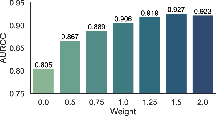
(a) Ablation on high-frequency importance

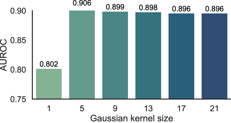
(b) Ablation on Gaussian kernel sizes

Figure 4: Ablation on high-frequency importance and Gaussian kernel sizes in VAE. CIFAR-10 is the in-distribution data. Results are averaged over all OOD test datasets.

Ablation on the Gaussian kernel sizes.

Recall that the Gaussian kernel is adopted to induce the cf Section 3.1). The kernel size controls the tradeoff between the high-level structures and texture details. We train VAEs with different Gaussian kernel sizes on CIFAR-10, and evaluate the OOD detection performance respectively. The average AUROC across all OOD datasets is shown in Figure 4 (down). Results show that FRL is not sensitive to the choice of kernel size when it is sufficiently large.

FRL is compatible with alternative high-frequency representations.

In FRL, the Gaussian kernel aims at exploiting high-frequency information to enhance OOD detection performance. In addition to the Gaussian kernel, we show that other mechanisms for extracting high-frequency information can also be used in our framework, such as Fourier transformation with FFT [4] and Wavelet transformation using Haar wavelets [53]. Table 4 shows that the performance of all three methods exploiting high-frequency information surpasses the baseline Input Complexity by a large margin. On GLOW, the Wavelet transformation shows slight improvement over the Gaussian kernel.

Table 4: AUROC values for OOD detection under three high frequency representation forms in VAE, GLOW, and PixelCNN++ when CIFAR-10 is the in-distribution dataset, here results are averaged upon all OOD datasets.

High-frequency form	VAE	GLOW	PixelCNN++
None (Input Complexity)	0.798	0.727	0.877
Gaussian kernel	0.906	0.802	0.920
Fourier transformation	0.860	0.809	0.893
Wavelet transformation	0.894	0.826	0.905

FRL achieves strong results with efficient inference.

We show the number of images processed per second under different approaches for VAE in Table 2 when CIFAR-10 serves as the ID dataset. Specifically, FRL can process 169.3 images per second, while the current best generative approach LR(E) can only process 1.3 images per second, which is far from the real-time inference requirement. Furthermore, LR(E) can be much slower when deployed into real-world datasets with higher resolution. For example, as we show in Section 4.3, LR(E) processes 0.3 images per second on a larger dataset CelebA, which is 147$\times$ slower than our method.

5 Related Work

Out-of-distribution Detection

Machine learning models commonly make the closed-world assumption that the training and testing data distributions match. However, this assumption rarely holds in the real world, where a model can encounter out-of-distribution data. OOD detection is thus critical to enabling safe model deployment. The idea of OOD detection is to reject samples from the unfamiliar distribution, and handle those with caution. A comprehensive survey on OOD detection is provided in [52]. Existing OOD approaches can be categorized broadly into generative-based and discriminative-based approaches. The key difference between the two is the presence or absence of label information. Below we review literature in the two categories separately.

Generative-based OOD Detection

Generative modeling aims at estimating the likelihood of the given input [20]. Generative models can be roughly categorized into three types: auto-encoders [20], flow-based models [37], and autoregressive [35, 38] models. Autoencoder-based models [1] aim at reconstructing the input using the encoder-decoder architecture. Flow-based models [37] such as GLOW [37] adopt the invertible network architectures to derive the likelihood from the latent variable. Autoregressive models like PixeCNN [35] and PixelCNN++ [38] sequentially predict the likelihood for each element, and optimize the joint likelihood over all elements. The generative model is a natural choice for OOD detection. Intuitively, the likelihood of the in-distribution samples should be higher than that of the out-of-distribution samples. However, Nalisnick et al. [32] revealed that deep generative models trained on CIFAR-10 unexpectedly assign a higher likelihood to certain OOD datasets such as MNIST. Subsequent works propose different test-time measurements such as Likelihood Ratio [36], Input Complexity [39], and Likelihood Regret [48]. To better understand the phenomenon, several recent studies [55, 31, 21] showed that current generative models overfit to the training set, especially when the structures of the images are simple. In this paper, we propose to use high-frequency information to regularize the training of deep generative models, which in turn improves the test-time OOD detection substantially.

Discriminative-based OOD Detection

A parallel line of the OOD detection approach relies on discriminative-based models, which utilize label information. The phenomenon of neural networks’ overconfidence in out-of-distribution data is first revealed by Nguyen et al. [34], which makes softmax probability confidence unable to effectively distinguish between the ID and OOD data. Subsequent works attempted to improve the OOD uncertainty estimation by using OpenMax score [2], deep ensembles [24], ODIN score [15, 27], and the energy score [28]. Besides model-based OOD detection, several works explored using features information to discriminative ID vs OOD data. For example, Mahalanobis distance [26] uses the multivariate Gaussian model to estimate the feature space, then apply the distance score in the feature space to detect OOD samples. However, a drawback of discriminative-based OOD detection methods is that they don’t directly model the likelihood of the input $p(\mathbf{x})$. In other words, the OOD scores can be less interpretable from a likelihood perspective.

Frequency Analysis in Deep Learning

Frequency domain analysis is widely used in traditional image processing [13, 7, 42, 17, 12]. The key idea of frequency analysis is to map the pixels from the Euclidean space to a frequency space, based on the changing speed in the spatial domain. Several works tried to bridge the connection between deep learning and frequency analysis [49, 5, 50, 51, 44, 30]. Wang et al. [43] found that the high-frequency components are useful in explaining the generalization of neural networks. Durall et al. [10] observed that the images generated by GANs are heavily distorted in high-frequency parts, where they introduced a spectral regularization term to the loss function to alleviate this problem. Recent work FDIT [4] indicated that the high-frequency information better enhances the identity preserving in the image generation process. To the best of our knowledge, no prior work has explored using frequency-domain analysis for the out-of-distribution detection task. In this work, we propose a novel frequency regularized OOD detection framework, which demonstrates its superiority in terms of both OOD detection performance and computational efficiency.

6 Conclusion

In this work, we propose a novel frequency-regularized learning (FRL) framework for out-of-distribution detection, which jointly estimates the likelihood of the pixel-space input and high-frequency information. Unlike existing generative modeling approaches, FRL guides the model to focus on semantically relevant features during training, where high-frequency information helps regularize the model in training. FRL can be flexibly used for common generative model architectures including VAE, GLOW, and PixelCNN++. Experiments on both common benchmark and a large-scale evaluation show that FRL effectively improves the OOD detection performance while preserving the generative capability. Extensive ablation studies further validate the effectiveness of our approach both qualitatively and quantitatively. We hope our work will increase the attention toward a broader view of frequency-based approaches for uncertainty estimation.

Supplementary Material

Appendix A OOD Detection Results on Fashion-MNIST

Table 5 shows the OOD detection results on Fashion MNIST in VAE. Our method FRL achieves a strong performance across all OOD datasets, with an average AUROC score of 0.976. Among the challenging OOD datasets for Input Complexity (IC) [39], such as LSUN and Noise, FRL achieves nearly optimal OOD detection performance.

Table 5: AUROC values for OOD Detection in VAE when Fashion-MNIST is the in-distribution dataset.

OOD Dataset	NLL	LRatio	LR(Z)	LR(E)	IC	FRL
	[32]	[36]	[48]	[48]	[39]	(ours)
SVHN	0.998	0.546	0.795	1.000	0.999	1.000
LSUN	1.000	0.991	0.691	0.995	0.508	1.000
CIFAR-10	1.000	0.929	0.751	0.999	0.905	1.000
MNIST	0.165	0.864	0.589	0.961	0.932	0.909
KMNIST	0.630	0.967	0.620	0.992	0.629	0.887
Omniglot	1.000	1.000	0.725	1.000	1.000	1.000
NotMNIST	0.979	0.965	0.721	1.000	0.909	0.988
Noise	1.000	1.000	0.603	0.999	0.490	1.000
Constant	0.938	0.416	0.761	0.998	1.000	1.000
Average	0.857	0.853	0.695	0.994	0.819	0.976
Num img/$s$ ($\uparrow$)	557.0	284.4	2.6	1.3	360.0	262.0
$T_{\text{inference}}(s)$ ($\downarrow$)	0.0018	0.0035	0.3779	0.7419	0.0028	0.0038

Appendix B Diagnosing the failure cases of prior approaches

Though the complexity score (IC) mitigates many failure cases compared to directly employing NLL, IC struggles with a few special failure cases. In particular, we show the score distribution when the Noise dataset serves as the OOD dataset for VAE trained on Fashion-MNIST (ID). Shown in Figure 5, the scores for Noise lie in the middle of the scores for Fashion-MNIST, which is undesirable. This is because the image code length is only the approximation of the complexity score. In contrast, FRL enables effective model regularization, which better distinguishes Noise and Fashion-MNIST data. Moreover, we also notice that FRL produces a more concentrated score distribution for ID data (green shade), benefiting the OOD detection.

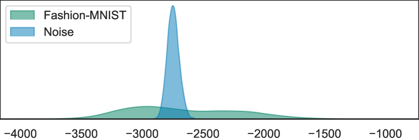
(a) IC

(b) FRL

Figure 5: The distribution of OOD scores $S_{F}(\mathbf{x})$ for Fashion-MNIST and Noise dataset when Fashion-MNIST serves as the in-distribution dataset. Two panels denote the distributions under IC and FRL, respectively.

Appendix C Ablations on Gaussian Kernel Sizes

Similar to the ablation studies on Gaussian kernels in VAE, we train GLOW [19] and PixelCNN++ [38] models with different kernel sizes on CIFAR-10, and evaluate the OOD detection performance respectively. The average AUROC across all OOD datasets is shown in Figure  6. Results also suggest that FRL is not sensitive to the choice of kernel size.

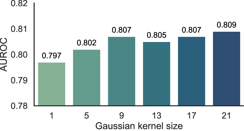
(a) GLOW

(b) PixelCNN++

Figure 6: Ablation on Gaussian kernel sizes in GLOW and PixelCNN++. CIFAR-10 is the in-distribution data. Results are averaged over all OOD test datasets.

Appendix D Model Overview for PixelCNN++

The overview of PixelCNN++ [38] under FRL is shown in Figure 7. For each pixel, four channels ($\mathbf{x}_{H}$, R, G, B) are modeled successively, with $\mathbf{x}_{H}$ conditioned on (R, G, B), B conditioned on (R, G), and G conditioned on R. Here $\mathbf{x}_{H}$ denotes the high-frequency features given input $\mathbf{x}$ in FRL. The sequential prediction is achieved by splitting the feature maps at every layer of the network into four and adjusting the centre values of the mask tensors. The 256 possible values for each channel are then modeled using the softmax.

PixelCNN++ [38] consists of a stack of masked convolution layers that takes an $N\times N\times 4$ image as input and produces $N\times N\times 4\times 256$ predictions as output. The use of convolutions allows the predictions for all the pixels to be made in parallel during training. During sampling the predictions are sequential: every time a pixel is predicted, it is fed back into the network to predict the next pixel.

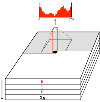
Figure 7: Overview of PixelCNN++ under FRL.

Appendix E Model Overview for GLOW

The overview of GLOW [19] under FRL is shown in Figure 8.

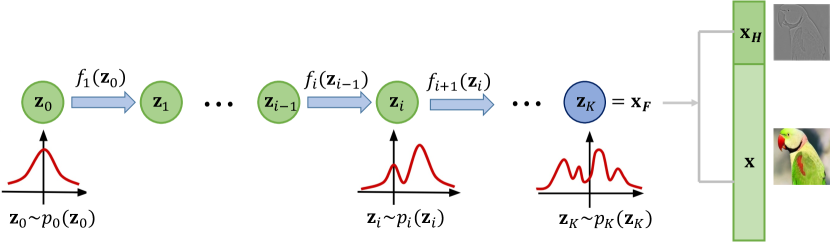
Figure 8: Overview of the GLOW under FRL.

Figure 9: The qualitative reconstruction results for CelebA under VAE. (a) shows the source images randomly picked from CelebA. (b) Shows the reconstruction results under the vanilla VAE training scheme. (c) shows the results when VAE is trained jointly with pixel level input and the high frequency information.

GLOW consists of a series of steps of flow, combined in a multi-scale architecture [19]. Each step of flow consists of actnorm followed by an invertible $1\times 1$ convolution and a coupling layer. The GLOW model has a depth of flow $K$, which maps the latent variable $\mathbf{z}_{0}$ to input $\mathbf{x}_{F}$.

Appendix F More Training Details

We provide more details for training on each of the architecture: VAE, GLOW and PixelCNN+.

(1) We train VAE using learning rate $1\times 10^{-3}$ and Adam optimizer [18]. The learning rate is decayed by half every 30 epochs. The encoder of VAEs consists of four convolutional layers of kernel size 4, strides 2 without biases. The decoder of VAEs has a symmetric structure to the encoder, reconstructing the image pixel-wise. In VAE, the distribution of the latent code prior $p(\mathbf{z})$ and the variational posterior $q_{\phi}(\mathbf{z}|\mathbf{x})$ are set to be Gaussians. In our experiments, the dimension for the latent code $p(\mathbf{z})$ is set to be 200 for CIFAR-10 and CelebA, and 100 for Fashion-MNIST.

(2) For GLOW, the number of the hidden channels is 400 for CIFAR-10 and 200 for Fashion-MNIST. 3-layer networks are used in the coupling blocks. We use two blocks of 16 flows for Fashion-MNIST, and three blocks of 8 flows with multi-scale for CIFAR-10.

(3) In PixelCNN++, all residual layers use 192 feature maps and a dropout rate of 0.5.

Appendix G Qualitative Results of Image Generation

FRL not only significantly improves the OOD detection performance, but also preserves the generative capability. Figures 9 shows the visualizations of the reconstruction results under the vanilla VAE and FRL for CelebA, where the reconstruction quality of FRL is not compromised. We further quantitatively measure the reconstruction results in Table 6. FRL achieves stronger results measured by both pixel-level and perception level metrics, including mean-square error (MSE), mean absolute error (MAE), peak signal-to-noise ratio (PSNR), and SSIM.

Table 6: CelebA reconstruction performance, measured by the image reconstruction quality between vanilla VAE and FRL. Evaluation metrics includes mean-square error (MSE), mean absolute error (MAE), peak signal-to-noise ratio (PSNR) [8], and SSIM [45]. $\uparrow$ means that higher value represents better image quality, and vice versa.

	vanilla VAE	FRL
MSE $\downarrow$	0.0041	0.0037
MAE $\downarrow$	0.0352	0.0337
PSNR $\uparrow$	24.657	25.097
SSIM $\uparrow$	0.7662	0.7806

Appendix H Social Impact

This paper aims to improve the reliability and safety of modern neural networks, particularly generative model families. Our study can lead to direct benefits and societal impacts when deploying machine learning models in the real world. Our work does not involve any human subjects or violation of legal compliance. We do not anticipate any potentially harmful consequences. Through our study and releasing our code, we hope to raise stronger research and societal awareness towards the problem of out-of-distribution detection.

References

- [1] Jinwon An and Sungzoon Cho. Variational autoencoder based anomaly detection using reconstruction probability. Special Lecture on IE, 2(1):1–18, 2015.
- [2] Abhijit Bendale and Terrance Boult. Towards open set deep networks. In Computer Vision and Pattern Recognition (CVPR), 2016 IEEE Conference on. IEEE, 2016.
- [3] Ronald Newbold Bracewell and Ronald N Bracewell. The Fourier transform and its applications, volume 31999. McGraw-Hill New York, 1986.
- [4] Mu Cai, Hong Zhang, Huijuan Huang, Qichuan Geng, Yixuan Li, and Gao Huang. Frequency domain image translation: More photo-realistic, better identity-preserving. In Proceedings of the IEEE/CVF International Conference on Computer Vision (ICCV), pages 13930–13940, October 2021.
- [5] Yunpeng Chen, Haoqi Fan, Bing Xu, Zhicheng Yan, Yannis Kalantidis, Marcus Rohrbach, Shuicheng Yan, and Jiashi Feng. Drop an octave: Reducing spatial redundancy in convolutional neural networks with octave convolution. In IEEE International Conference on Computer Vision, 2019.
- [6] Mircea Cimpoi, Subhransu Maji, Iasonas Kokkinos, Sammy Mohamed, and Andrea Vedaldi. Describing textures in the wild. In Proceedings of the IEEE Conference on Computer Vision and Pattern Recognition (CVPR), June 2014.
- [7] James W Cooley. The re-discovery of the fast fourier transform algorithm. Microchimica Acta, 93(1):33–45, 1987.
- [8] Johannes F De Boer, Barry Cense, B Hyle Park, Mark C Pierce, Guillermo J Tearney, and Brett E Bouma. Improved signal-to-noise ratio in spectral-domain compared with time-domain optical coherence tomography. Optics letters, 28(21):2067–2069, 2003.
- [9] Li Deng. The mnist database of handwritten digit images for machine learning research. IEEE Signal Processing Magazine, 29(6):141–142, 2012.
- [10] Ricard Durall, Margret Keuper, and Janis Keuper. Watch your up-convolution: Cnn based generative deep neural networks are failing to reproduce spectral distributions. In Proceedings of the IEEE/CVF Conference on Computer Vision and Pattern Recognition, 2020.
- [11] Borko Furht, editor. Portable Network Graphics (Png), pages 729–729. Springer US, Boston, MA, 2008.
- [12] W Morven Gentleman and Gordon Sande. Fast fourier transforms: for fun and profit. In Proceedings of the November 7-10, 1966, fall joint computer conference, pages 563–578, 1966.
- [13] Michael Heideman, Don Johnson, and Charles Burrus. Gauss and the history of the fast fourier transform. IEEE ASSP Magazine, 1(4):14–21, 1984.
- [14] Irina Higgins, Loic Matthey, Arka Pal, Christopher Burgess, Xavier Glorot, Matthew Botvinick, Shakir Mohamed, and Alexander Lerchner. beta-vae: Learning basic visual concepts with a constrained variational framework. In International Conference on Learning Representations, 2017.
- [15] Y. C. Hsu, Y. Shen, H. Jin, and Z. Kira. Generalized odin: Detecting out-of-distribution image without learning from out-of-distribution data. In 2020 IEEE/CVF Conference on Computer Vision and Pattern Recognition (CVPR), pages 10948–10957, 2020.
- [16] Rui Huang and Yixuan Li. Mos: Towards scaling out-of-distribution detection for large semantic space. In Proceedings of the IEEE/CVF Conference on Computer Vision and Pattern Recognition (CVPR), pages 8710–8719, June 2021.
- [17] Steven G Johnson and Matteo Frigo. A modified split-radix fft with fewer arithmetic operations. IEEE Transactions on Signal Processing, 55(1):111–119, 2006.
- [18] Diederik P Kingma and Jimmy Ba. Adam: A method for stochastic optimization. arXiv preprint arXiv:1412.6980, 2014.
- [19] Diederik P. Kingma and Prafulla Dhariwal. Glow: Generative flow with invertible 1x1 convolutions. In NeurIPS, pages 10236–10245, 2018.
- [20] Diederik P. Kingma and Max Welling. Auto-encoding variational bayes. In Yoshua Bengio and Yann LeCun, editors, 2nd International Conference on Learning Representations, ICLR 2014, Banff, AB, Canada, April 14-16, 2014, Conference Track Proceedings, 2014.
- [21] Polina Kirichenko, Pavel Izmailov, and Andrew Gordon Wilson. Why normalizing flows fail to detect out-of-distribution data. In Hugo Larochelle, Marc’Aurelio Ranzato, Raia Hadsell, Maria-Florina Balcan, and Hsuan-Tien Lin, editors, Advances in Neural Information Processing Systems 33: Annual Conference on Neural Information Processing Systems 2020, NeurIPS 2020, December 6-12, 2020, virtual, 2020.
- [22] Alex Krizhevsky, Geoffrey Hinton, et al. Learning multiple layers of features from tiny images. Master’s thesis, Department of Computer Science, University of Toronto, 2009.
- [23] Brenden M Lake, Ruslan Salakhutdinov, and Joshua B Tenenbaum. Human-level concept learning through probabilistic program induction. Science, 350(6266):1332–1338, 2015.
- [24] Balaji Lakshminarayanan, Alexander Pritzel, and Charles Blundell. Simple and scalable predictive uncertainty estimation using deep ensembles. In Proceedings of the 31st International Conference on Neural Information Processing Systems, NIPS’17, page 6405–6416, 2017.
- [25] Alex Lamb, Asanobu Kitamoto, David Ha, Kazuaki Yamamoto, Mikel Bober-Irizar, and Tarin Clanuwat. Deep learning for classical japanese literature. In NIPS Workshop on Machine Learning for Creativity and Design, 2018.
- [26] Kimin Lee, Kibok Lee, Honglak Lee, and Jinwoo Shin. A simple unified framework for detecting out-of-distribution samples and adversarial attacks. In NeurIPS, pages 7167–7177, 2018.
- [27] Shiyu Liang, Yixuan Li, and R Srikant. Enhancing the reliability of out-of-distribution image detection in neural networks. International Conference on Learning Representations (ICLR), 2018.
- [28] Weitang Liu, Xiaoyun Wang, John Owens, and Yixuan Li. Energy-based out-of-distribution detection. Advances in Neural Information Processing Systems (NeurIPS), 2020.
- [29] Ziwei Liu, Ping Luo, Xiaogang Wang, and Xiaoou Tang. Deep learning face attributes in the wild. In Proceedings of International Conference on Computer Vision (ICCV), December 2015.
- [30] Zhenhua Liu, Jizheng Xu, Xiulian Peng, and Ruiqin Xiong. Frequency-domain dynamic pruning for convolutional neural networks. In Advances in Neural Information Processing Systems, 2018.
- [31] Vaishnavh Nagarajan, Anders Andreassen, and Behnam Neyshabur. Understanding the failure modes of out-of-distribution generalization. In International Conference on Learning Representations, 2021.
- [32] Eric Nalisnick, Akihiro Matsukawa, Yee Whye Teh, Dilan Gorur, and Balaji Lakshminarayanan. Do deep generative models know what they don’t know? In International Conference on Learning Representations, 2019.
- [33] Yuval Netzer, Tao Wang, Adam Coates, Alessandro Bissacco, Bo Wu, and Andrew Y. Ng. Reading digits in natural images with unsupervised feature learning. In NIPS Workshop on Deep Learning and Unsupervised Feature Learning 2011, 2011.
- [34] Anh Nguyen, Jason Yosinski, and Jeff Clune. Deep neural networks are easily fooled: High confidence predictions for unrecognizable images. In Proceedings of the IEEE conference on computer vision and pattern recognition, pages 427–436, 2015.
- [35] Aäron van den Oord, Nal Kalchbrenner, Oriol Vinyals, Lasse Espeholt, Alex Graves, and Koray Kavukcuoglu. Conditional image generation with pixelcnn decoders. In Proceedings of the 30th International Conference on Neural Information Processing Systems, NIPS’16, page 4797–4805, Red Hook, NY, USA, 2016. Curran Associates Inc.
- [36] Jie Ren, Peter J. Liu, Emily Fertig, Jasper Snoek, Ryan Poplin, Mark Depristo, Joshua Dillon, and Balaji Lakshminarayanan. Likelihood ratios for out-of-distribution detection. In H. Wallach, H. Larochelle, A. Beygelzimer, F. d'Alché-Buc, E. Fox, and R. Garnett, editors, Advances in Neural Information Processing Systems, volume 32. Curran Associates, Inc., 2019.
- [37] Danilo Jimenez Rezende and Shakir Mohamed. Variational inference with normalizing flows. In Proceedings of the 32nd International Conference on International Conference on Machine Learning - Volume 37, ICML’15, page 1530–1538. JMLR.org, 2015.
- [38] Tim Salimans, Andrej Karpathy, Xi Chen, and Diederik P. Kingma. Pixelcnn++: Improving the pixelcnn with discretized logistic mixture likelihood and other modifications. In 5th International Conference on Learning Representations, ICLR 2017, Toulon, France, April 24-26, 2017, Conference Track Proceedings. OpenReview.net, 2017.
- [39] Joan Serrà, David Álvarez, Vicenç Gómez, Olga Slizovskaia, José F. Núñez, and Jordi Luque. Input complexity and out-of-distribution detection with likelihood-based generative models. In International Conference on Learning Representations, 2020.
- [40] Christopher Torrence and Gilbert P Compo. A practical guide to wavelet analysis. Bulletin of the American Meteorological society, 79(1):61–78, 1998.
- [41] Grant Van Horn, Oisin Mac Aodha, Yang Song, Yin Cui, Chen Sun, Alex Shepard, Hartwig Adam, Pietro Perona, and Serge Belongie. The inaturalist species classification and detection dataset. In Proceedings of the IEEE Conference on Computer Vision and Pattern Recognition (CVPR), June 2018.
- [42] Charles Van Loan. Computational frameworks for the fast Fourier transform. SIAM, 1992.
- [43] Haohan Wang, Xindi Wu, Zeyi Huang, and Eric P Xing. High-frequency component helps explain the generalization of convolutional neural networks. In Proceedings of the IEEE/CVF Conference on Computer Vision and Pattern Recognition, 2020.
- [44] Yunhe Wang, Chang Xu, Shan You, Dacheng Tao, and Chao Xu. Cnnpack: Packing convolutional neural networks in the frequency domain. In Advances in Neural Information Processing Systems, 2016.
- [45] Zhou Wang, Alan C Bovik, Hamid R Sheikh, and Eero P Simoncelli. Image quality assessment: from error visibility to structural similarity. IEEE Transactions on Image Processing, 13(4):600–612, 2004.
- [46] Han Xiao, Kashif Rasul, and Roland Vollgraf. Fashion-mnist: a novel image dataset for benchmarking machine learning algorithms, 2017.
- [47] Jianxiong Xiao, James Hays, Krista A Ehinger, Aude Oliva, and Antonio Torralba. Sun database: Large-scale scene recognition from abbey to zoo. In 2010 IEEE computer society conference on computer vision and pattern recognition, pages 3485–3492. IEEE, 2010.
- [48] Zhisheng Xiao, Qing Yan, and Yali Amit. Likelihood regret: An out-of-distribution detection score for variational auto-encoder. In H. Larochelle, M. Ranzato, R. Hadsell, M. F. Balcan, and H. Lin, editors, Advances in Neural Information Processing Systems, volume 33, pages 20685–20696. Curran Associates, Inc., 2020.
- [49] Kai Xu, Minghai Qin, Fei Sun, Yuhao Wang, Yen-Kuang Chen, and Fengbo Ren. Learning in the frequency domain. In Proceedings of the IEEE/CVF Conference on Computer Vision and Pattern Recognition, 2020.
- [50] Zhi-Qin John Xu. Frequency principle: Fourier analysis sheds light on deep neural networks. Communications in Computational Physics, 28(5):1746–1767, Jun 2020.
- [51] Zhi-Qin John Xu, Yaoyu Zhang, and Yanyang Xiao. Training behavior of deep neural network in frequency domain. In Tom Gedeon, Kok Wai Wong, and Minho Lee, editors, Neural Information Processing, pages 264–274, Cham, 2019. Springer International Publishing.
- [52] Jingkang Yang, Kaiyang Zhou, Yixuan Li, and Ziwei Liu. Generalized out-of-distribution detection: A survey. arXiv preprint arXiv:2110.11334, 2021.
- [53] Jaejun Yoo, Youngjung Uh, Sanghyuk Chun, Byeongkyu Kang, and Jung-Woo Ha. Photorealistic style transfer via wavelet transforms. In IEEE International Conference on Computer Vision, 2019.
- [54] Fisher Yu, Yinda Zhang, Shuran Song, Ari Seff, and Jianxiong Xiao. Lsun: Construction of a large-scale image dataset using deep learning with humans in the loop. CoRR, abs/1506.03365, 2015.
- [55] Lily H. Zhang, Mark Goldstein, and Rajesh Ranganath. Understanding failures in out-of-distribution detection with deep generative models, 2021.
- [56] Bolei Zhou, Agata Lapedriza, Aditya Khosla, Aude Oliva, and Antonio Torralba. Places: A 10 million image database for scene recognition. IEEE Transactions on Pattern Analysis and Machine Intelligence, 2017.