An Integer L-shaped Method for Dynamic Order Dispatching in Autonomous Last-Mile Delivery with Demand Uncertainty

Abstract

Given the potential to significantly reduce the cost and time in last-mile delivery, autonomous delivery solutions via delivery robots or unmanned aerial vehicles have received increasing attention. This paper studies the dynamic order dispatching problem in an autonomous last-mile delivery system with intrinsic demand uncertainty. We consider a rolling order-fulfilment context and formulate a two-stage stochastic programming to take into account both existing unfulfilled orders and future incoming requests to minimize the total expected delays in package delivery. The considered uncertainty includes the stochastic arrival of delivery requests, their types, locations/delivery distances, and associated penalties for late delivery. Due to the constrained service capacity, the size of the problem grows exponentially as the number of simulated scenarios increases. In this study, we propose a modified integer L-shaped method, which (i) significantly reduces the number of nodes in the branching tree, and (ii) simplifies the computation of optimality cuts. The computational results show that these two modifications improve the average running time by roughly 10 times and 1,000 times compared to the non-customized L-shaped method and the classic branch-and-bound method, respectively. The linearly growing computational speed in response to the number of scenarios enables it as a viable solution for large-sized problems in reality.

Keywords - last-mile delivery; dynamic order dispatch; two-stage stochastic programming; integer L-shaped

1 Introduction

Given its utmost convenience provided to consumers, online-enabled delivery service has been rising steadily in the past decades and expanded its coverage to an extensive list of discretionary and non-discretionary products and services, including goods, meals, groceries, medications, among others. The availability and popularization of these delivery channels have deeply reshaped people’s lifestyles (Shi and Xu,, 2021). Especially during the COVID-19 pandemic, more and more people gave up shopping at brick-and-mortar stores and shifted toward online channels having packages delivered directly to their front doors. Facing the explosive demand for last-mile delivery, the delivery industry has eyed autonomous solutions using drones and delivery robots. According to a report by Verified Market Research (Verified Market Research,, 2021), the global autonomous delivery robots market size was valued around USD 24.3 million in 2019 and is expected to grow up to USD 236.59 million by 2027. More and more deliver companies and online retailers including FedEx and Amazon are joining the game and testing drones and robots for last-mile delivery (Banker, Steve,, 2022). These low-capacity autonomous vehicles have been demonstrated to significantly reduce the vehicle miles traveled as well as the energy consumption related to package delivery (Figliozzi,, 2020).

For a delivery system, there are two core logistical processes: order dispatch and vehicle routing. The former refers to the management control of receiving, storing, picking, packing, and shipping orders at depots, whilst the latter manages delivery fleets to travel back and forth between the depots and spatially distributed delivery points. This study focuses on the process of order dispatch to a group of unit-capacity autonomous vehicles. We consider customers’ order requests arrive dynamically at a central depot and accumulate until a decision epoch, in which the manager decides the set of orders to fulfill and then service them in batch through a wave of autonomous delivery. The decision epochs are carried out periodically with constant intervals. At each epoch, there are two categories of information available to the manager. One is the set of unfulfilled requests that remain open with known delivery destinations and penalties for late delivery. The other is the profile of potential requests that may arrive in the next few waves. The penalty for the late delivery of each request is assumed proportional to the delivery distance/cost and its elapsed time in the system after passing the committed time of delivery.

Given the fixed service capacity, the dynamic and stochastic demand requests may temporarily exceed the full capacity of autonomous vehicles at a depot. Accordingly, in those cases, a number of requests will need to be delayed to join the future epochs for service. Then, the manager should decide which requests to put off by trading off between the tasks on the pipeline and potential arrivals in the future. She needs to make a priori decisions at each epoch and take correction actions via recourse rules in future waves. The fundamental consideration falls between serving for distant customers with higher penalties or close ones with lower penalties, constrained by the furthest distance delivery vehicles can travel in the current and future waves. To assist with the decision-making in such contexts, this paper formulates a stochastic optimization model with a two-stage structure to tackle the dynamic dispatching problem at each epoch. A customized integer L-Shaped method by reducing the branching nodes and modifying the optimality cuts is developed to achieve better computing efficiency.

The remainder of this paper is organized as follows. The next section first reviews the related work. The third section introduces our problem setting of dispatching unit-capacity autonomous delivery vehicles for spatially distributed tasks and formulates a two-stage stochastic program for tackling the problem with intrinsic demand uncertainty. The integer L-shaped method as well as our modifications are then detailed, followed by the computational results that compare the performance of our customized method to the classic integer L-shaped method and the branch-and-bound method. At the end, the last section concludes the paper.

2 Related Work

Existing work has tackled the dynamic order dispatching using dynamic programming by modeling the multi-staged problems as Markov decision process (MDP) (Klapp et al.,, 2018). Many other studies formulated dynamic routing problems in MDP and customized various heuristic algorithms for efficient solutions (Kok et al.,, 2010; Ulmer et al.,, 2020). Given the nature of MDP as a sequential decision-making, reinforcement learning approaches were used more and more often to solve the dynamic problems in logistics (Nazari et al.,, 2018; Mao and Shen,, 2018). In general, due to the exponentially growing complexity in the dimensions of states, decisions, and scenario realizations, dynamic programming faces challenges in dealing with large-scale stochastic problems. In this paper, we formulate a two-stage stochastic program to solve the dynamic dispatching problem of unit-capacity autonomous delivery vehicles (ADVs). The two stages respectively account for the dispatching decisions and system conditions in the current wave and the future waves to come. By iteratively rolling out this program at each epoch, the dispatching problem can be solved dynamically to minimize the total penalties occurred over time.

The adopted approach falls within the scope of the stochastic vehicle routing problems (SVRPs) where the stochastic components are typically modeled either as a chance constrained program (CCP) or a stochastic program with recourse (SPR). In CCPs, the failure of delivery is allowed and the probability of failure is constrained to be below a certain threshold (Raff,, 1983). The more common formulation is through SPR, whose aim is to determine the first-stage solution that minimizes the expected cost of both the two stages, i.e., the realized cost of the first-stage solution plus the expected net cost of the recourse. The uncertainty in SPRs can originate from stochastic demands (Bertsimas,, 1992; Erera et al.,, 2010) or stochastic travel time (Laporte et al.,, 1992; Taş et al.,, 2013; Venkatachalam et al.,, 2018). In this study, the uncertain demand sums up the random arrival of delivery requests as well as the various aspects of properties associated with each request including its location and urgency. Since we hold all requests during each period and consider them altogether at the ending epoch, the random arrivals of requests are then transferred into the random number of requests at each delivery wave.

The stochastic or dynamic vehicle routing problem is usually modeled as a mixed or pure integer stochastic program. The most common way is to transfer it to an equivalent deterministic problem by solving the sample average. The basic idea is to approximate the expected demand-related costs through sample-average estimates under a finite set of scenarios that are assumed to be independent and identically distributed (i.i.d.) samples of uncertain elements. When the number of sample scenarios is sufficiently large, the yielded optimal solution will converge to the true optimum almost surely (Bertsimas et al.,, 2018). However, accurately solving the problems with heavily simulated scenarios is often time-consuming, and effective methods are needed to accelerate the solution procedure and obtain feasible solutions in a reasonable time. For example, hybrid genetic algorithm has been applied to solve the SVRP (Berger and Barkaoui,, 2003), that approaches a suboptimal solution by exploiting the similarities between a set of parallel solutions. Another more robust solution is the integer L-shaped method, an exact decomposition algorithm applicable to a wide range of stochastic integer programs with recourse. It is implemented with branch and cut that iteratively updates the first stage solution using the generated optimality cut obtained through the lower bound on the expected cost of recourse (Laporte and Louveaux,, 1993). Compared to the brutal solution of deterministic counterparts, this decomposition method has been demonstrated to perform exceedingly well in many applications with a large number of scenarios, such as vehicle routing problem (Laporte et al.,, 2002), location and network restoration problem (Sanci and Daskin,, 2021) and generalized assignment problem (Albareda-Sambola et al.,, 2006).

3 Problem Formulation

3.1 Background on Two-Stage Stochastic Program

In general, the two-stage stochastic program with recourse is defined with the following form:

(P1):

$$\min\bm{c}^{T}\bm{x}+\mathbb{E}_{\xi}\left[\mathbb{Q}(\bm{x},\xi)\right]$$ (1a)

s.t.

$$A\bm{x}=b$$ (1b)

$$\bm{x}\geq 0$$ (1c)

where

$$\mathbb{Q}(\bm{x},\xi)=\min\{q(\xi)^{T}\bm{y}(\xi)\ |\ W(\xi)\bm{y}(\xi)=h(\xi)-T(\xi)\bm{x},\ \bm{y}(\xi)\geq 0\}$$ (1d)

In problem (P1), $\bm{x}$ and $\bm{y}(\xi)$ are the first-stage and second-stage decision variables; $\xi$ represents the set of random factors, and $\mathbb{E}_{\xi}$ denotes the mathematical expectation with respect to $\xi$. In the most general case, all parameters of the recourse function $\mathbb{Q}(\bm{x},\xi)$, including $\bm{q,\ W,\ h}$, and $\bm{T}$, can be made responsive to the realization of $\xi$. The first-stage decisions $\bm{x}$ is made taking into account the full randomness of $\xi$, whereas the second-stage or recourse (corrective) actions $\bm{y}$ will base on the decisions admitted in the first stage as well as the revealed realization of $\xi$ Birge and Louveaux, (2011).

3.2 Problem Statement

We consider the dynamic order dispatching problem that send out ADVs for spatial delivery. There is a set of customer nodes $N$ consisting of all possible delivery destinations and a set of arcs $A$ connecting between the depot and customer nodes. The ADVs are considered unit-capacity and can only serve one customer at one time. On delivery of a package at its destination, the ADV will return to the depot and then proceed with the next request. A request can stay open for a length of $|T|$ waves, after which it will be cancelled and result in a devastating penalty. For each request $i$, the penalty incurred at wave $t(\in T)$ after its generation is predetermined as $c_{t}^{i}$. New orders add continuously to the system with known delivery distances and penalties, and existing orders are served and removed from the system during each delivery wave.

The dispatching decisions at each epoch of the above dynamic rolling problem can be materialized as a two-stage problem. There is an accumulation of requests $I$ remaining open in the system. For each of these existing requests $i\in I$, we know its exact delivery distance, generated time, and time-moving penalties. Then, at each epoch, the first-stage decision variables are $x_{0}^{i}$ and $u_{0}^{i,l}$, which are both binary indicators for whether request $i$ will be selected for delivery in the current wave and whether to be taken by ADV $l\in L$. A set of potential requests $J$ may appear in the several periods afterward. In this problem, we define the second-stage tasks $J$ as the set of new tasks accumulated within $|T|$ waves and denote $a^{j,\xi}$ as the arriving time (wave) of request $j\in J$. The second stage involves four primary sets of decision variables: $x_{t}^{i,\xi}$ and $y_{t}^{j,\xi}$ are two sets of binary variables indicating whether a request $i\in I$ from the first stage or a newly arriving request $j\in J$ will be serviced in wave $t$ in the second stage; $u_{t}^{i,l,\xi}$ and $v_{t}^{j,l,\xi}$ are their corresponding variables determining the responsible ADVs. Assume that all the requests are reachable by an ADV in a wave, i.e., the length of each wave is long enough to allow an ADV to travel at least back and forth from the furthest possible delivery point. The interval between any two consecutive epochs is predetermined and fixed.

The stochasticity in the second stage originates from the number of requests realized in $J$, as well as their arriving epoch $\{a^{j,\xi}\}$, delivery distance $\{d^{j,\xi}\}$, and time-moving penalties $\{c^{j,\xi}_{t}\}$. Because the two-stage formulation does not recognize a variable set of $J$, i.e., $\left|J\right|$ is fixed for different scenarios in $\xi$, we use a trick to allow variations in the number of requests arriving in the second stage. For example, if normal requests are distributed within a delivery range of 10 miles, we then simulate a fixed number of requests in the range of e.g., -5 to 10 miles by including an extra range for each scenario. Those cases outside the normal range will be treated as invalid requests and served immediately by a virtual ADV with unlimited flying range in each wave. Thus, even though the size of $J$ is fixed, this treatment allows the number of valid orders being random in different scenarios.

3.3 Mathematical Formulation

Table 1: Notation list of sets, variables, parameters and functions

Notation	Description
Sets
$i\in I$	Existing requests in the current delivery wave
$j\in J$	Potential requests arriving in the future waves
$l\in L$	Fleet of ADVs
$t\in T$	Retention time of tasks
$\omega\in\Omega$	Scenario realization in the future waves
Deterministic Parameters
$c_{t}^{i}$	Penalty for a first-stage task delivered in the $t^{\text{th}}$ wave
$D$	Maximum distance an ADV can travel in a delivery wave
$d^{i}$	Delivery distance of task $i$
$M$	Sufficiently large number
Uncertain Parameters
$c^{j,\omega}_{t}$	Penalty for a second-stage task $j$ delivered in the $t^{\text{th}}$ wave in realization $\omega$
$d^{j,\omega}$	Delivery distance of task $j$ in realization $\omega$
$a^{j,w}$	Arriving time (epoch) of the task $j$ in realization $\omega$
First-Stage Binary Variables
$x_{0}^{i}$	Whether task $i$ is delivered in the current wave
$u_{0}^{i,l}$	Whether task $i$ is delivered in the current wave by ADV $l$
Second-Stage Binary Variables
$x_{t}^{i,\omega}\ (y_{t}^{j,\omega})$	Whether task $i(j)$ would be delivered in the $t^{\text{th}}$ wave
$u_{t}^{i,l,\omega}\ (v_{t}^{j,l,\omega})$	Whether task $i(j)$ would be delivered by ADV $l$ in the $t^{\text{th}}$ wave
$v^{j,0,\omega}$	Whether task $j$ would be delivered by the virtual ADV once it is generated
Functions
$\mathbb{Q}(\cdot)$	Second-stage recourse function

The physical processes detailed above for the dispatching of ADVs at each epoch can be expressed into a two-stage structure as follows (A notational glossary is enclosed in Table 1 for reference):

(P2):

$$\min_{x,u\in\mathds{B}}\ \sum_{i\in I}c^{i}_{0}\cdot x_{0}^{i}+\mathbb{E}_{\xi}\left[\mathbb{Q}(\bm{x_{0}},\xi)\right]$$ (2a)

s.t.

$$x_{0}^{i}=\sum_{l\in L}u_{0}^{i,l} \forall i\in I$$ (2b)

$$\sum_{i\in I}d^{i}\cdot u_{0}^{i,l}\leq D \forall l\in L$$ (2c)

where

$$\mathbb{Q}(\bm{x_{0}},\xi)=\min_{\bm{x,y,u,v\in\mathds{B}}}\ \sum_{i\in I}\sum_{t\in T+1}c^{i}_{t}\cdot x_{t}^{i,\xi}+\sum_{j\in J}\sum_{t\in T+1}c^{j,\xi}_{t}\cdot y_{t}^{j,\xi}$$ (2d)

s.t.

$$x_{0}^{i}+\sum_{t\in T+1}x_{t}^{i,\xi}=1 \forall i\in I$$ (2e)

$$\sum_{t\in T+1}y_{t}^{j,\xi}=1 \forall j\in J$$ (2f)

$$x_{t}^{i,\xi}=\sum_{l\in L}u_{t}^{i,l,\xi} \forall i\in I,t\in T$$ (2g)

$$y_{t}^{j,\xi}=\sum_{l\in L}v_{t}^{j,l,\xi}+v^{j,0,\xi}\cdot\mathbbm{1}(a^{j,\xi}=t) \forall j\in J,t\in T$$ (2h)

$$M\cdot(1-y^{j,\xi}_{t})\geq a^{j,\xi}-t \forall j\in J,t\in T+1$$ (2i)

$$\sum_{i\in I}d^{i}\cdot u_{t}^{i,l,\xi}+\sum_{j\in J}d^{j,\xi}\cdot v_{t}^{j,l,\xi}\leq D \forall l\in L,t\in T$$ (2j)

$$d^{j,\xi}\geq-M\cdot v^{j,0,\xi} \forall j\in J$$ (2k)

$$d^{j,\xi}\leq M\cdot\left(1-v^{j,0,\xi}\right) \forall j\in J$$ (2l)

In the optimization problem, the objective function (2a) is to minimize the sum of penalties from the first-stage delivery and the expected penalties during the future waves (i.e., the recourse function in (2d); Constraints (2b,g) ensure if request $i\in I$ is selected for service in a wave, it is taken only by one ADV; and if it is not served, no ADV will be committed; Constraints (2c,j) guarantee for each ADV $l\in L$, its total delivery distance in each wave cannot exceed its maximum travel range per wave. For the second-stage constraints, (2e) and (2f) limit that all requests will be either serviced in one of the delivery waves in $T$ or cancelled at the $(|T|+1)^{\text{th}}$ wave. Equation (2h) ensures that for any request $j\in J$ realized in the second stage, it will be served by either a real ADV $l\in L$ or the virtual ADV immediately on its arrival if the request is invalid. Constraint (2i) restrains that all the requests can only be serviced or cancelled after its generation. The last two Big-M constraints (2k,l) limit the invalid and valid tasks to be only taken care of by the virtual and real ADVs, respectively.

4 Methodology

Solving the above optimization problem (P2) requires the computation of the expected values outputted by the recourse function $\mathbb{Q}(\bm{x},\xi)$. In nature, this characterizes an integral in extremely high dimensions that is challenging, if not impossible, to compute. The most common solution is to solve an equivalent deterministic sample-average problem by sampling a discrete set of realizations $\Omega$ instead of a continuously distributed random events $\xi$ Birge and Louveaux, (2011). Therefore, in this section, we propose a Sample Average Approximation (SAA) formulation, which is directly solvable but maybe time-consuming using the basic integer optimization method. An integer L-shaped method is further customized to efficiently handle the extensive form of SAA.

4.1 Sample Average Approximation

The SAA is based on the Monte Carlo simulation and deterministic optimization techniques. Instead of computing the expectation of recourse function value $\mathbb{Q}(\bm{x},\xi)$ in problem (P2), we employ a finite set of scenarios $\Omega$ and rewrite the problem as follows:

(P3):

$$\min_{x,u\in\mathds{B}}\ \sum_{i\in I}c^{i}_{0}\cdot x_{0}^{i}+\frac{1}{\left|\Omega\right|}\sum_{\omega\in\Omega}(\sum_{i\in I}\sum_{t\in T+1}c^{i}_{t}\cdot x_{t}^{i,\omega}+\sum_{j\in J}\sum_{t\in T+1}c^{j,\omega}_{t}\cdot y_{t}^{j,\omega})$$ (3a)

s.t.

$$x_{0}^{i}=\sum_{l\in L}u_{0}^{i,l} \forall i\in I$$ (3b)

$$\sum_{i\in I}d^{i}\cdot u_{0}^{i,l}\leq D \forall l\in L$$ (3c)

$$x_{0}^{i}+\sum_{t\in T+1}x_{t}^{i,\omega}=1 \forall i\in I,\omega\in\Omega$$ (3d)

$$\sum_{t\in T+1}y_{t}^{j,\omega}=1 \forall j\in J,\omega\in\Omega$$ (3e)

$$x_{t}^{i,\omega}=\sum_{l\in L}u_{t}^{i,l,\omega} \forall i\in I,t\in T,\omega\in\Omega$$ (3f)

$$y_{t}^{j,\omega}=\sum_{l\in L}v_{t}^{j,l,\omega}+v^{j,0,\omega}\cdot\mathbbm{1}(a^{j,w}=t) \forall j\in J,t\in T,\omega\in\Omega$$ (3g)

$$M\cdot(1-y^{j,\omega}_{t})\geq a^{j,\omega}-t \forall j\in J,t\in T+1,\omega\in\Omega$$ (3h)

$$\sum_{i\in I}d^{i}\cdot u_{t}^{i,l,\omega}+\sum_{j\in J}d^{j,\omega}\cdot v_{t}^{j,l,\omega}\leq D \forall l\in L,t\in T,\omega\in\Omega$$ (3i)

$$d^{j,\omega}\geq-M\cdot v^{j,0,\omega} \forall j\in J,\omega\in\Omega$$ (3j)

$$d^{j,\omega}\leq M\cdot\left(1-v^{j,0,\omega}\right) \forall j\in J,\omega\in\Omega$$ (3k)

Based on the historical data, the set $\Omega$ contains simulated i.i.d. scenarios from the random events $\xi$. When the size of $\Omega$ is adequately large, the SAA formulation of problem (P3) can well approximate the expected objective value in Equation (2a). The optimal solution of problem (P3) would also approach the true optimum of problem (P2). However, it can be observed that as the set $\Omega$ grows, directly solving the SAA formulation (P3) becomes quite time-consuming because both the numbers of decision variables and constraints increase accordingly. Therefore, a decomposition method is needed to reduce the computational complexity for better scalability.

4.2 General Framework of the L-shaped Method

Before heading to our customization, let us first briefly introduce the general idea of the classical L-shaped method based on the general form (P1). Taking advantage of the separable structure between the first and second stages, the L-shaped method aims to build an outer linearization of the second-stage recourse function. This outer linearization depicts the shape of $\mathbb{L}(\bm{x})=\mathbb{E}_{\xi}\mathbb{Q}(\bm{x},\xi)$ based on a given $\bm{x}$. Now, we introduce a new variable $\theta$ to create a series of lower bound cutting planes to successively approximate $\mathbb{L}(\bm{x})$. Through the successful addition of optimality cuts, $\theta$ keeps increasing to better approximate $\mathbb{L}(\bm{x})$ until an optimal solution $\mathbb{L}(\bm{x}^{*})=\theta^{*}$ is found. Thus, problem (P1) can be transferred as follows Birge and Louveaux, (2011):

(P4):

$$\min z=\bm{c}^{T}\bm{x}+\theta$$ (4a)

s.t.

$$Ax=b$$ (4b)

$$D_{l}\bm{x}\geq d_{l} l=1,2,\ldots,r$$ (4c)

$$E_{l}\bm{x}+\theta\geq e_{l} l=1,2,\ldots,s$$ (4d)

$$\bm{x}\geq 0$$ (4e)

This problem (P4) is called the master problem. It consists of finding a proposal first-stage solution $\bm{x}^{v}$ in $v^{\text{th}}$ iteration, and sent to the second stage for calculating two types of cuts added to the master problem. Then, these two types of cuts are sequentially added: (i) feasibility cuts (4c) ensure the second-stage problem is feasible when current first-stage solution is sent to it, and (ii) optimality cuts (4d), which are linear approximations of $\mathbb{L}(\bm{x})$. For our problem (P3), no matter whether an order is served or not in the first stage, it is always feasible for the second stage problem to be solved. So, there is no feasibility cut needed to be considered in our problem. For the optimality cuts, we will describe the integer optimality cuts for the binary first-stage variables in the next section.

4.3 Customized Integer L-Shaped Method

This section presents a decomposition-based branch-and-cut algorithm adapting from the integer L-shaped method developed by (Laporte and Louveaux,, 1993). The integer L-shaped method couples the branching scheme widely used in integer programming with the concept of optimality cuts from the L-shaped method. In each iteration, we need to solve the master problem (P4), if the solution is not integer, we create two new branches on one of the fractional variable following the usual branch and bound procedure. If the solution satisfies the integrality constraint, we need to check the condition $\theta^{v}\geq\mathbb{L}(\bm{x}^{v})$ for the current solution of $\bm{x}$ and $\theta$ during this iteration $v$. If it is not satisfied, the following optimality cut, developed by (Laporte and Louveaux,, 1993), will be added to the master problem:

$$\theta\geq(\mathbb{L}(\bm{x})-L)(\sum_{i\in S}x_{i}-\sum_{i\notin S}x_{i})-(\mathbb{L}(\bm{x})-L)(\left|S\right|-1)+L$$ (5)

Here, $x_{i}=1$, $i\in S$, and $x_{i}=0$, $i\notin S$ are the first-stage feasible solution solved in this iteration. $\mathbb{L}(\bm{x})=\mathbb{E}_{\xi}\mathbb{Q}(\bm{x},\xi)$ is the corresponding second-stage recourse function value. $L$ is the lower bound for all $\mathbb{L}(\bm{x})$, i.e., $L\leq\min_{\bm{x}}\{\mathbb{L}(\bm{x})\ |A\bm{x}=b,\bm{x}\in X\}$. In our problem, to find a lower bound $L$ as large as possible, we can set the first-stage variables $x_{0}^{i}=1$ for all orders, meaning there is no remaining orders to be passed to the second stage. The resultant $\mathbb{L}(\bm{x_{0}})$ serves a feasible lower bound.

Different from the original treatment proposed by (Laporte and Louveaux,, 1993), one modification we adopt here is that instead of considering all first-stage variables, we only include the cuts related to $x_{0}^{i}$ and ignore $u_{0}^{i,l}$, i.e.,

$$\theta\geq(\mathbb{L}(\bm{x_{0}})-L)(\sum_{i\in S}x_{0}^{i}-\sum_{i\notin S}x_{0}^{i})-(\mathbb{L}(\bm{x_{0}})-L)(\left|S\right|-1)+L$$ (6)

where $x_{0}^{i}=1$, $i\in S$, and $x_{0}^{i}=0$, $i\notin S$ are the first-stage binary variables determining whether task $i$ is delivered. Because in our problem, the remaining requests are the only factor from the first stage that will influences the value of second-stage recourse function. How the requests selected in the first stage are delivery by ADVs does not interact with the second-stage decisions. We can see that the term $(\sum_{i\in S}x_{0}^{i}-\sum_{i\notin S}x_{0}^{i})$ is constantly less than or equal to $\left|S\right|$. Under the condition when all $x_{0}^{i}=1$, which is how we obtained our lower bound $L$, the right hand side of Equation (6) equals to $\mathbb{L}(\bm{x_{0}})$, and thus $\theta\geq\mathbb{L}(\bm{x_{0}})$ is the cut we need to add to meet the condition we checked before. In all other cases, $(\sum_{i\in S}x_{0}^{i}-\sum_{i\notin S}x_{0}^{i})$ is smaller than or equal to $\left|S\right|-1$, which implies that the right hand side of Equation (6) takes a value smaller than or equal to $L$. This is also valid since $\theta$ is an approximation of second-stage value and should always be larger than the lower bound of second-stage value.

Comparing to the original cut proposed by (Laporte and Louveaux,, 1993), the key point why it works here is the calculation of second-stage recourse function value $\mathbb{L}(\bm{x})$ only depends on $\bm{x_{0}}$ but not $\bm{u_{0}}$ in our problem. Another point worthy of attention is the need to ensure the current solution of $\bm{x_{0}}$ is feasible, i.e., there exists a set of non-negative integer solution of $\bm{u_{0}}$ to satisfy the $\bm{x_{0}}$. With these conditions hold, our modified cut is valid and transforms the master problem for (P2) as follows:

(MP):

$$\min_{x,u\in\mathds{B}}\ z=\sum_{i\in I}c^{i}_{0}\cdot x_{0}^{i}+\theta$$ (7a)

s.t.

$$x_{0}^{i}=\sum_{l\in L}u_{0}^{i,l} \forall i\in I$$ (7b)

$$\sum_{i\in I}d^{i}\cdot u_{0}^{i,l}\leq D \forall l\in L$$ (7c)

$$\theta\geq(\mathbb{L}(\bm{x_{0}^{v}})-L)(\sum_{i\in S^{v}}x_{0}^{i}-\sum_{i\notin S^{v}}x_{0}^{i})-(\mathbb{L}(\bm{x_{0}^{v}})-L)(\left|S\right|-1)+L \forall v\in V$$ (7d)

where $\mathbb{L}(\bm{x_{0}})=\mathbb{E}_{\omega\in\Omega}\left[\mathbb{Q}(\bm{x_{0}},\omega)\right]$ calculates the expectation from solving $\left|\Omega\right|$ subproblems (SP) as follows,

(SP):

$$\mathbb{Q}(\bm{x_{0}},\omega)=\min_{\bm{x,y,u,v\in\mathds{B}}}\ \sum_{i\in I}\sum_{t\in T+1}c^{i}_{t}\cdot x_{t}^{i,\omega}+\sum_{j\in J}\sum_{t\in T+1}c^{j,\omega}_{t}\cdot y_{t}^{j,\omega}$$ (8a)

s.t.

$$x_{0}^{i}+\sum_{t\in T+1}x_{t}^{i,\omega}=1 \forall i\in I$$ (8b)

$$\sum_{t\in T+1}y_{t}^{j,\omega}=1 \forall j\in J$$ (8c)

$$x_{t}^{i,\omega}=\sum_{l\in L}u_{t}^{i,l,\omega} \forall i\in I,t\in T$$ (8d)

$$y_{t}^{j,\omega}=\sum_{l\in L}v_{t}^{j,l,\omega}+v^{j,0,\omega}\cdot\mathbbm{1}(a^{j,w}=t) \forall j\in J,t\in T$$ (8e)

$$M\cdot(1-y^{j,\omega}_{t})\geq a^{j,\omega}-t \forall j\in J,t\in T+1$$ (8f)

$$\sum_{i\in I}d^{i}\cdot u_{t}^{i,l,\omega}+\sum_{j\in J}d^{j,\omega}\cdot v_{t}^{j,l,\omega}\leq D \forall l\in L,t\in T$$ (8g)

$$d^{j,\omega}\geq-M\cdot v^{j,0,\omega} \forall j\in J$$ (8h)

$$d^{j,\omega}\leq M\cdot\left(1-v^{j,0,\omega}\right) \forall j\in J$$ (8i)

Given the above elucidation, we now assemble the components into the following procedure, which demonstrates swift and effective convergence in our implementation:

1. Set the best objective value $\bar{z}=\infty$. The value of $\theta$ is set to $-\infty$ and is ignored in the initialization computation. A single pendant node corresponding to the master problem of (MP) without any optimality cut (7d) is first created, and append it as the root node to the branch-and-bound tree.

2. Select a pendant node in the branching tree. If none exists, stop.

3. Solve the current master problem.

   • If the current problem has no feasible solution, fathom the current node and go to Step 1.

   • Otherwise, let ($\bm{x_{0}^{v}}$, $\theta^{v}$) be the current optimal solution and go to Step 3.

4. • If current master problem objective is larger than the best objective obtained already ($\sum_{i\in I}c^{i}_{0}\cdot x_{0}^{i,v}+\theta^{v}\geq\bar{z}$), no need to continue branch on this node, fathom the current problem and go to Step 1.

   • Otherwise, go to Step 4.

5. Check the integrality status of the current problem.

   • If one of $\bm{x_{0}}$ violates the integrality restriction, create two new branches following the usual branch and bound procedure. Append the two new nodes to the branching tree, and go to Step 1.

   • Else if $\bm{x_{0}}$ is integer, $\bm{u_{0}^{l}}$ cannot be integer, which means some orders can only be served by multiple drones, fathom this infeasible node, and go to Step 1.

   • Else if $\bm{x_{0}}$ is integer, $\bm{u_{0}^{l}}$ can be integer, which means current solution of $\bm{x_{0}}$ and $\bm{u_{0}^{l}}$ is feasible, then go to Step 5.

6. Compute $\mathbb{L}(\bm{x_{0}})$ and $z^{v}=\sum_{i\in I}c^{i}_{0}\cdot x_{0}^{i,v}+\mathbb{L}(\bm{x_{0}})$. If $z^{v}<\bar{z}$, update $\bar{z}=z^{v}$ and record current $\bm{x_{0}}$ and $\bm{u_{0}^{l}}$ as the best solution so far. Go to Step 6.

7. • If $\theta\geq\mathbb{L}(\bm{x_{0}})$, then fathom this current node and return to Step 1.

   • Otherwise, impose one optimality cut of (6) to the master problem of all pendant nodes in the tree, and return to Step 2.

5 Computational Results

In this section, we evaluate the performance of our customized integer L-shaped method for solving the dispatch problem (P3) and compare it to the performance achieved by the non-customized L-shaped and non-decomposition branch-and-bound (BnB) methods. Because all three methods are exact algorithms targeting the global minimum, we report their computational time (CPU time) and branching tree sizes instead of the quality of optimal solutions from solving various instances. All three methods are coded in Python and deployed with Gurobi 9.5 on MacBook Pro with Apple M1 Pro Chip 3.22 GHz and 16 GB RAM.

5.1 Data Generation

Table 2: Notation list of simulated problem parameters

Notation	Description
$\left|I\right|$	Number of first-stage requests
$\left|J\right|$	Number of second-stage requests
$\left|L\right|$	Number of ADVs
$\left|T\right|$	Lifespan of requests
$\left|\Omega\right|$	Number of simulated scenarios
$N_{vars}$	Number of variables for the SAA formulation (P3)

A number of simulated data sets are generated for numerical experiments (Table 2 overviews the notations of parametric settings in simulations). For the following experiments, the lifespan of requests is set to three waves, i.e., all requests will be cancelled with a high penalty if they are not answered in three epochs. Thus, in each epoch, no existing tasks can be generated four waves before. This setting can be extended to any longer lifespan. Meanwhile, the number of ADVs is fixed in our model but can be relaxed in future work. The delivery distances of requests in the second stage are simulated with uniform distribution between -5 and 10 miles to enable randomness in the number of valid requests. The number of variables $N_{vars}$ is computed from all the other parametric setting to indicate the problem size. Lastly, we cap the running time for each experimental instance at 10,000 seconds to avoid the endless wait.

5.2 Result Comparison

Table 3: Running time and branching tree size comparison of three methods
($\left|I\right|=6$, $\left|J\right|=6$, $\left|L\right|=3$, $\left|\Omega\right|=3$, $N_{vars}=366$)

Runs	Running Time (seconds)
	Customized L-shaped	Non-customized L-shaped	Branch-and-Bound
1	3	23	$>$10000
2	3	23	$>$10000
3	2	22	744
4	2	71	1
5	2	17	4130
6	2	16	497
7	3	26	113
8	2	9	$>$10000
9	2	21	2642
10	3	70	21
Average	2.4	29.8	$>$3814.8
St. Dev	0.5	20.8	$>$4234.7
Runs	Number of Branching Tree Nodes
	Customized L-shaped	Non-customized L-shaped	Branch-and-Bound
1	95	2353	$>$1324807
2	101	2913	$>$1419775
3	103	2771	136065
4	117	5077	57
5	105	2133	690085
6	111	2193	94779
7	113	3501	21573
8	107	1141	$>$1458713
9	93	2205	434643
10	125	5231	3689
Average	107.0	2951.8	$>$558518.6
St. Dev	9.3	1244.5	$>$589495.2

On completion of a series of numerical experiments, we compare the running time (in seconds) and the number of branching tree nodes exhibited during the solutions of the three methods. The number of branching tree nodes is defined as the total number of nodes computed or added to the branching tree. When one variable is integer, two new nodes are appended to the branching tree, and the number of nodes reported adds by two. In general, a larger sized branching tree would imply longer computation time. But the relation is not linear. The L-shaped method requires additional time to construct the optimality cuts for each node, whereas the branch-and-bound can move to the next branching more quickly. Consequently, both metrics are reported as indicators for computational efficiency.

Table 3 first reports the results on instances, with $\left|I\right|=6$, $\left|J\right|=6$, and $\left|L\right|=3$. It is clear that even for a small problem with $\left|\Omega\right|=3$ scenarios, solving the SAA formulation of (P3) using branch-and-bound is rather time-consuming and unstable. With 366 integer variables, the average running time is already over an hour, with 3 out of 10 cases exceeding the 10,000-second cap. Each scenario added will roughly result in a hundred additional integer variables. So the running time using branch-and-bound will explode for a large number of scenarios. In contrast, both the customized and non-customized L-shaped methods can significantly reduce the running time and branching tree size to a computable degree. Later, more examples will demonstrate the superiority of the L-shaped methods in solving stochastic problems with a large number of scenarios. Since the BnB method is infeasible to solve problems with hundreds of integer variables, it will be excluded from the comparisons hereafter.

5.3 Sensitivity to the Number of Scenarios

We next present the sensitivity analyses with respect to the number of simulated scenarios. Figure 1 and 2 show the box plots of running time and number of branching tree nodes for the customized and non-customized L-shaped methods. Ten replications are simulated at each scenario size. Table 4 and 5 in Appendix A provide the detailed results of each instance. We can see for both of the running time and number of branching tree nodes metrics, the customized L-shaped method improves over 10 times on average comparing to the non-customized counterpart. Since the optimal solution will converge to the true value when the number of simulated scenarios $\left|\Omega\right|$ is sufficiently large, the customized L-shaped method acts as a more viable solution in this regard.

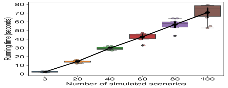
(a) Customized L-shaped

(b) Non-customized L-shaped

Figure 1: Comparisons of running time w.r.t number of simulated scenarios for (a) Customized L-shaped and (b) Non-customized L-shaped

Figure 1 shows that the running time of both the customized and non-customized L-shaped methods increases linearly with respect to the number of scenarios increases. For the customized method, the average running time increases by $\{15.2,13.2,14.1,13.8\}$ seconds, with a very small range of fluctuations, for every 20 (or close to 20) extra scenarios simulated. It is also worth noting that although the variance of the CPU time enlarges with the number of scenarios, the customized L-shaped method generally performs more robust across all level of scenarios.

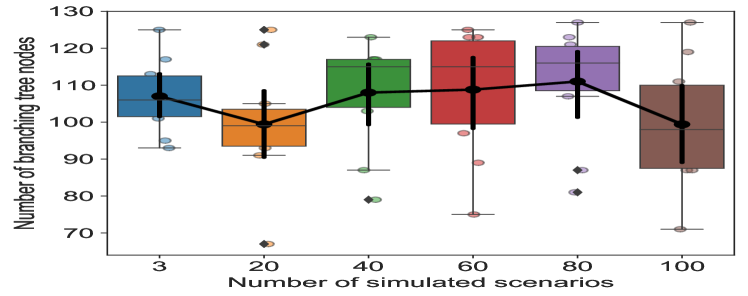
(a) Customized L-shaped

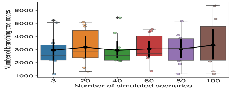
(b) Non-customized L-shaped

Figure 2: Comparisons of number of branching tree nodes w.r.t number of simulated scenarios for (a) Customized L-shaped and (b) Non-customized L-shaped

As shown in Figure 2, the number of branching tree nodes remains almost the same for both methods. The reason is that the branching tree size mostly depends on the number of variables in the first stage. Increasing the number of scenarios will only affect the speed of computing optimality cuts, where one of its element $\mathbb{L}(\bm{x_{0}})=\mathbb{E}_{\omega\in\Omega}\left[\mathbb{Q}(\bm{x_{0}},\omega)\right]$ requires solving $\left|\Omega\right|$ subproblems (SP). This is also why the running time is linear in the number of scenarios, because the time spent computing optimality cuts is linearly proportional to the scenario size. In addition, by considering the first-stage variables $\bm{x_{0}}$ and $\bm{u_{0}^{l}}$ separately, our customized method could fathom more infeasible nodes through each iteration (in Step 4, specifically) and thus compute fewer nodes in the branching tree. Combined with the other modification of simplified optimality cuts, the customized method improves significantly in solving the order dispatching problem.

5.4 Sensitivity to the Number of Requests

Another dimension that may affect the performance of our customized L-shaped method are the number of requests. Figure 3 and 4 presents our customized L-shaped method’s sensitivity in running time and branching tree size with respect to the number of requests in the first stage $\left|I\right|$ and second stage $\left|J\right|$, respectively. Please see Tables 6 and 7 in Appendix B for the detailed results of individual instances. Figure 3 first shows that both the running time and number of branching tree nodes grow roughly exponentially with the number of first-stage requests. The increments of running time for $\left|I\right|=\{6,8,10,12,14\}$ exhibit an increasing manner of $\{121.6,433.4,710.1,2911.7\}$ seconds. Since the branching algorithm works on the first-stage variable $\bm{x_{0}}$, such an exponential growth can be anticipated. Comparatively, the running time grows linearly in the number of second-stage requests $\left|J\right|$, with a constant 10-second increment for every two more requests. For both $\left|I\right|$ and $\left|J\right|$, adding two more requests would involve an additional one thousand integer variables approximately. However, increasing $\left|J\right|$ will not affect the size of the branching tree, while increasing $\left|I\right|$ causes a sharp increase in the number of nodes to compute. Thus, the running time of the customized method presents an exponential pattern on $\left|I\right|$ but increases only linearly on $\left|J\right|$.
 

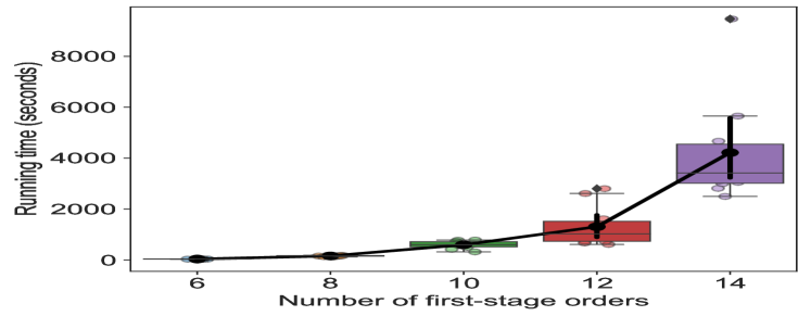
(a) Running Time (seconds)

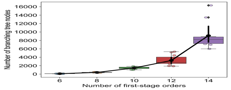
(b) Number of Branching Tree Nodes

Figure 3: (a) Running time (seconds) and (b) Number of branching tree nodes w.r.t number of first-stage orders $\left|I\right|$ for customized L-shaped method

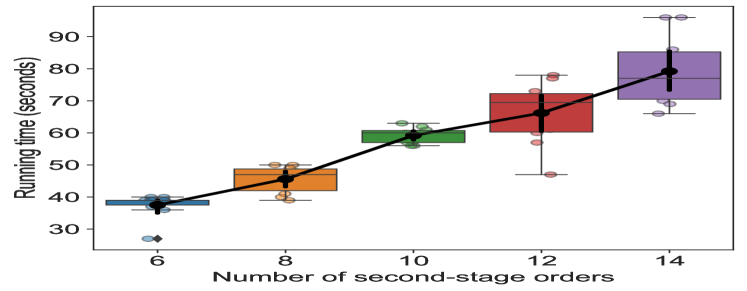
(a) Running Time (seconds)

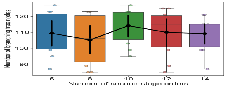
(b) Number of Branching Tree Nodes

Figure 4: (a) Running time (seconds) and (b) Number of branching tree nodes w.r.t number of second-stage orders $\left|J\right|$ for customized L-shaped method

6 Conclusion

This paper studies the dynamic order dispatching problem in the context of autonomous last-mile delivery with demand uncertainty. A two-stage stochastic program is formulated catering to the rolling process of order dispatching, with the current wave considered as the first stage and future waves gathered in the second stage. The uncertainty involves the stochastic arrival time of orders, their delivery distances, and corresponding penalties for late delivery. By considering the expectation of future second stage penalty, we can obtain an optimal dispatching schedule of ADVs in the current wave. Afterward, we can move on to the next wave, and dynamically solve this problem in a rolling base. To effectively solve this two-stage problem, we propose an exact solution approach modified from the integer L-shaped method developed by (Laporte and Louveaux,, 1993). The computational results indicate that our customized integer L-shaped method improves over 10 times and 1,000 times in average running time comparing to the non-customized L-shaped and classical branch-and-bound, respectively. The sensitivity analysis suggests that the running time of our algorithm is linearly correlated to the number of scenarios simulated, which provides a viable solution when the number of scenarios is sufficiently large. Other empirical results show that the solution time highly depends on the size of the branching tree created, i.e., growing exponentially with respect to the number of first-stage variables, but remains insensitive to the size of second-stage variables.

Future research directions may include: (i) considering the vehicle routing problems after the order dispatching stage; (ii) modeling the planning-level decisions, such as to determine the number of delivery vehicles; (iii) involving specific technological constraints for delivery vehicles on their capacitated transportation, charging, and potential collaborations with high-capacity trucks; (iv) enhancing the operational objectives accounting for the environmental aspects of societal concerns.

Appendix A Computational Results for Sensitivity to the Number of Scenarios

Table 4: Sensitivity of scenarios number for customized L-shaped method
($\left|I\right|=6$, $\left|J\right|=6$, $\left|L\right|=3$)

Runs	Running Time (seconds)
	$\left|\Omega\right|=20$	$\left|\Omega\right|=40$	$\left|\Omega\right|=60$	$\left|\Omega\right|=80$	$\left|\Omega\right|=100$
	($N_{vars}=2304$)	($N_{vars}=4584$)	($N_{vars}=6864$)	($N_{vars}=9144$)	($N_{vars}=11424$)
1	16	31	47	54	70
2	15	29	40	54	76
3	15	29	43	64	74
4	13	30	45	44	79
5	12	27	44	54	78
6	13	32	47	57	65
7	16	28	46	60	53
8	15	28	44	59	79
9	15	32	40	60	79
10	15	31	33	64	55
Average	14.5	29.7	42.9	57.0	70.8
St. Dev	1.2	1.7	4.1	5.6	9.4
Runs	Number of Branching Tree Nodes
	$\left|\Omega\right|=20$	$\left|\Omega\right|=40$	$\left|\Omega\right|=60$	$\left|\Omega\right|=80$	$\left|\Omega\right|=100$
	($N_{vars}=2304$)	($N_{vars}=4584$)	($N_{vars}=6864$)	($N_{vars}=9144$)	($N_{vars}=11424$)
1	91	117	123	107	91
2	95	115	113	81	119
3	121	115	89	127	105
4	99	87	107	113	127
5	99	107	117	113	71
6	105	79	125	119	107
7	93	123	123	121	89
8	67	103	119	87	87
9	99	117	97	123	87
10	125	117	75	119	111
Average	99.4	108.0	108.8	111.0	99.4
St. Dev	15.3	13.7	15.9	14.5	16.3

Table 5: Sensitivity of scenarios number for non-customized L-shaped method
($\left|I\right|=6$, $\left|J\right|=6$, $\left|L\right|=3$)

Runs	Running Time (seconds)
	$\left|\Omega\right|=20$	$\left|\Omega\right|=40$	$\left|\Omega\right|=60$	$\left|\Omega\right|=80$	$\left|\Omega\right|=100$
	($N_{vars}=2304$)	($N_{vars}=4584$)	($N_{vars}=6864$)	($N_{vars}=9144$)	($N_{vars}=11424$)
1	182	338	650	419	516
2	125	253	318	480	2858
3	179	214	494	1103	707
4	138	325	513	229	1561
5	74	209	337	405	1156
6	93	470	620	486	680
7	284	207	640	683	288
8	434	245	395	953	984
9	191	626	357	783	2310
10	384	543	175	1046	295
Average	208.4	343.0	449.9	658.7	1135.5
St. Dev	115.2	144.0	151.1	286.1	821.6
Runs	Number of Branching Tree Nodes
	$\left|\Omega\right|=20$	$\left|\Omega\right|=40$	$\left|\Omega\right|=60$	$\left|\Omega\right|=80$	$\left|\Omega\right|=100$
	($N_{vars}=2304$)	($N_{vars}=4584$)	($N_{vars}=6864$)	($N_{vars}=9144$)	($N_{vars}=11424$)
1	2557	2761	4357	2271	2089
2	2367	2509	2349	2149	6341
3	3551	2171	3005	5177	2461
4	2487	2603	2805	1151	6377
5	1325	2135	2643	1901	3091
6	1613	3165	4553	2565	2649
7	4913	2183	4429	3619	1339
8	5097	2185	2479	3877	2535
9	3125	5447	2589	4103	5343
10	4781	4275	1359	3737	1151
Average	3181.6	2943.4	3056.8	3055.0	3337.6
St. Dev	1296.5	1040.8	999.3	1170.2	1859.1

Appendix B Computational Results for Sensitivity to the Number of Requests

Table 6: Sensitivity of first-stage orders number $\left|I\right|$ for customized L-shaped method
($\left|J\right|=6$, $\left|L\right|=3$, $\left|\Omega\right|=50$)

Runs	Running Time (seconds)
	$\left|I\right|=6$	$\left|I\right|=8$	$\left|I\right|=10$	$\left|I\right|=12$	$\left|I\right|=14$
	($N_{vars}=5724$)	($N_{vars}=6632$)	($N_{vars}=7540$)	($N_{vars}=8448$)	($N_{vars}=9356$)
1	38	163	670	738	2813
2	36	152	562	897	5652
3	37	185	318	1230	3049
4	37	121	776	1616	2495
5	27	154	499	611	4198
6	39	181	618	666	3101
7	30	174	580	2611	4664
8	38	149	783	728	9468
9	32	163	416	2800	2999
10	39	127	731	1157	3732
Average	35.3	156.9	595.3	1305.4	4217.1
St. Dev	4.0	20.0	145.6	760.0	1977.3
Runs	Number of Branching Tree Nodes
	$\left|I\right|=6$	$\left|I\right|=8$	$\left|I\right|=10$	$\left|I\right|=12$	$\left|I\right|=14$
	($N_{vars}=5724$)	($N_{vars}=6632$)	($N_{vars}=7540$)	($N_{vars}=8448$)	($N_{vars}=9356$)
1	125	417	1711	2729	7147
2	97	457	1503	2819	13459
3	119	491	1049	2787	7995
4	117	339	1445	4455	5999
5	89	439	1271	1937	8927
6	67	309	1475	1891	7557
7	99	441	1535	5331	8483
8	123	403	1857	2441	16321
9	97	355	1007	5197	6981
10	115	375	1711	2723	8545
Average	104.8	402.6	1456.4	3231.0	9141.4
St. Dev	17.4	54.4	264.8	1214.3	3055.6

Table 7: Sensitivity of second-stage orders number $\left|J\right|$ for customized L-shaped method
($\left|I\right|=6$, $\left|L\right|=3$, $\left|\Omega\right|=50$)

Runs	Running Time (seconds)
	$\left|J\right|=6$	$\left|J\right|=8$	$\left|J\right|=10$	$\left|J\right|=12$	$\left|J\right|=14$
	($N_{vars}=5724$)	($N_{vars}=6724$)	($N_{vars}=7724$)	($N_{vars}=8724$)	($N_{vars}=9724$)
1	39	47	60	78	96
2	36	50	60	47	70
3	37	48	56	61	72
4	39	50	57	77	86
5	40	40	63	73	66
6	39	39	56	60	96
7	40	45	60	70	69
8	39	49	61	70	78
9	27	41	57	69	76
10	39	47	62	57	83
Average	37.5	45.6	59.2	66.2	79.2
St. Dev	3.7	4.0	2.4	9.3	10.3
Runs	Number of Branching Tree Nodes
	$\left|J\right|=6$	$\left|J\right|=8$	$\left|J\right|=10$	$\left|J\right|=12$	$\left|J\right|=14$
	($N_{vars}=5724$)	($N_{vars}=6724$)	($N_{vars}=7724$)	($N_{vars}=8724$)	($N_{vars}=9724$)
1	101	123	123	99	113
2	111	99	99	85	115
3	117	85	121	125	99
4	123	101	121	121	121
5	123	123	95	119	99
6	87	85	113	111	87
7	111	113	103	107	115
8	127	111	117	119	121
9	95	89	123	125	115
10	99	123	127	89	107
Average	109.4	105.2	114.2	110.0	109.2
St. Dev	12.8	14.8	10.7	13.9	10.5

References

- Albareda-Sambola et al., (2006) Albareda-Sambola, M., Van Der Vlerk, M. H., and Fernández, E. (2006). Exact solutions to a class of stochastic generalized assignment problems. European journal of operational research, 173(2):465–487.
- Banker, Steve, (2022) Banker, Steve (2022). Home delivery robots: Last mile gamechangers. https://www.forbes.com/sites/stevebanker/2022/05/01/home-delivery-robots-last-mile-gamechangers/?sh=41939f1030b, Last accessed on 2022-08-01.
- Berger and Barkaoui, (2003) Berger, J. and Barkaoui, M. (2003). A hybrid genetic algorithm for the capacitated vehicle routing problem. In Genetic and evolutionary computation conference, pages 646–656. Springer.
- Bertsimas et al., (2018) Bertsimas, D., Gupta, V., and Kallus, N. (2018). Robust sample average approximation. Mathematical Programming, 171(1):217–282.
- Bertsimas, (1992) Bertsimas, D. J. (1992). A vehicle routing problem with stochastic demand. Operations Research, 40(3):574–585.
- Birge and Louveaux, (2011) Birge, J. R. and Louveaux, F. (2011). Introduction to stochastic programming. Springer Science & Business Media.
- Erera et al., (2010) Erera, A. L., Morales, J. C., and Savelsbergh, M. (2010). The vehicle routing problem with stochastic demand and duration constraints. Transportation Science, 44(4):474–492.
- Figliozzi, (2020) Figliozzi, M. A. (2020). Carbon emissions reductions in last mile and grocery deliveries utilizing air and ground autonomous vehicles. Transportation Research Part D: Transport and Environment, 85:102443.
- Klapp et al., (2018) Klapp, M. A., Erera, A. L., and Toriello, A. (2018). The one-dimensional dynamic dispatch waves problem. Transportation Science, 52(2):402–415.
- Kok et al., (2010) Kok, A. L., Meyer, C. M., Kopfer, H., and Schutten, J. M. J. (2010). A dynamic programming heuristic for the vehicle routing problem with time windows and european community social legislation. Transportation Science, 44(4):442–454.
- Laporte et al., (1992) Laporte, G., Louveaux, F., and Mercure, H. (1992). The vehicle routing problem with stochastic travel times. Transportation science, 26(3):161–170.
- Laporte and Louveaux, (1993) Laporte, G. and Louveaux, F. V. (1993). The integer l-shaped method for stochastic integer programs with complete recourse. Operations research letters, 13(3):133–142.
- Laporte et al., (2002) Laporte, G., Louveaux, F. V., and Van Hamme, L. (2002). An integer l-shaped algorithm for the capacitated vehicle routing problem with stochastic demands. Operations Research, 50(3):415–423.
- Mao and Shen, (2018) Mao, C. and Shen, Z. (2018). A reinforcement learning framework for the adaptive routing problem in stochastic time-dependent network. Transportation Research Part C: Emerging Technologies, 93:179–197.
- Nazari et al., (2018) Nazari, M., Oroojlooy, A., Snyder, L., and Takác, M. (2018). Reinforcement learning for solving the vehicle routing problem. Advances in neural information processing systems, 31.
- Raff, (1983) Raff, S. (1983). Routing and scheduling of vehicles and crews: The state of the art. Computers & Operations Research, 10(2):63–211.
- Sanci and Daskin, (2021) Sanci, E. and Daskin, M. S. (2021). An integer l-shaped algorithm for the integrated location and network restoration problem in disaster relief. Transportation Research Part B: Methodological, 145:152–184.
- Shi and Xu, (2021) Shi, L. and Xu, Z. (2021). Dine in or take out? trends on restaurant service demand amid the covid-19 pandemic. Trends on Restaurant Service Demand amid the COVID-19 Pandemic (October 1, 2021).
- Taş et al., (2013) Taş, D., Dellaert, N., Van Woensel, T., and De Kok, T. (2013). Vehicle routing problem with stochastic travel times including soft time windows and service costs. Computers & Operations Research, 40(1):214–224.
- Ulmer et al., (2020) Ulmer, M. W., Goodson, J. C., Mattfeld, D. C., and Thomas, B. W. (2020). On modeling stochastic dynamic vehicle routing problems. EURO Journal on Transportation and Logistics, 9(2):100008.
- Venkatachalam et al., (2018) Venkatachalam, S., Sundar, K., and Rathinam, S. (2018). A two-stage approach for routing multiple unmanned aerial vehicles with stochastic fuel consumption. Sensors, 18(11):3756.
- Verified Market Research, (2021) Verified Market Research (2021). Autonomous delivery robots market. https://www.verifiedmarketresearch.com/download-sample/?rid=25692, Last accessed on 2022-08-01.