Improving Small Molecule Generation using Mutual Information Machine

Abstract

We address the task of controlled generation of small molecules, which entails finding novel molecules with desired properties under certain constraints. Here we introduce MolMIM, a probabilistic auto-encoder for small molecule drug discovery that learns an informative and clustered latent space. MolMIM is trained with Mutual Information Machine (MIM) learning and provides a fixed-size representation of variable-length SMILES strings. Since encoder-decoder models can learn representations with “holes” of invalid samples, here we propose a novel extension to the MIM training procedure which promotes a dense latent space and allows the model to sample valid molecules from random perturbations of latent codes. We provide a thorough comparison of MolMIM to several variable-size and fixed-size encoder-decoder models, demonstrating MolMIM’s superior generation as measured in terms of validity, uniqueness, and novelty. We then utilize CMA-ES, a naive black-box, and gradient-free search algorithm, over MolMIM’s latent space for the task of property-guided molecule optimization. We achieve state-of-the-art results in several constrained single-property optimization tasks and show competitive results in the challenging task of multi-objective optimization. We attribute the strong results to the structure of MolMIM’s learned representation which promotes the clustering of similar molecules in the latent space, whereas CMA-ES is often used as a baseline optimization method. We also demonstrate MolMIM to be favorable in a compute-limited regime.

1 Introduction

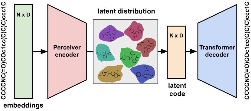
Figure 1: MolMIM is a Mutual Information Machine (MIM), a probabilistic encoder-decoder model with a fixed-size representation that learns an informative latent distribution clustered around similar molecules. N is the variable tokens number, D is the embeddings dimension, K is the fixed hidden length. Tokens are mapped to learnable embeddings.

The lead optimization stage of the drug discovery process is time consuming, labor intensive, and has a high rate of failure, requiring as much as three years and hundreds of millions of dollars for a single drug. This stage is focused on optimizing candidate molecules using the design-make-test cycle, in which scientists design new molecules based on available assay information, synthesize these molecules, and then test them in new assays. The risk and associated cost of this process makes it a high-value automation task in the drug discovery pipeline (Kim et al., 2020; Engkvist et al., 2021). Successful solutions to the automated design of small molecules can be directly applied to related challenges associated with other biological modalities, such as protein design (Berenberg et al., 2022) and optimization of guide RNA sequence for CRISPR systems (Chuai et al., 2018).

Controlled generation of small molecules entails finding a new molecule with certain properties and under some constraints (e.g., similarity to a reference molecule, Vamathevan et al. (2019)). Often these molecules are represented in a text-based encoding format called SMILES (Weininger, 1988). Efficient search of the space of molecules is a challenging problem due to the high dimensional and sparse nature of samples, where valid molecules are sparse given all possible combinations of legal characters in SMILES.

A common search method relies on genetic algorithms to modify a molecule’s SMILES representation using heuristics. Examples would be random mutations and hand-crafted rules (Sliwoski et al., 2014; Mahmood et al., 2021). The complex and high dimensional search space often leads to low sampling efficiency of such methods. In addition, the search is often based on ad hoc rules which require input from experts.

An alternative approach to automate this process with deep learning is to project the discrete molecules into a continuous space, wherein generation becomes sampling from a continuous space, and exploration becomes a manipulation of continuous vectors (Gómez-Bombarelli et al., 2018; Hoffman et al., 2022; Winter et al., 2019). Here, we follow that approach, focusing on learning a dense representation space that allows efficient sampling and exploration (Fig. 1).

In this paper we propose a novel probabilistic encoder-decoder model named MolMIM, a Mutual Information Machine (Livne et al., 2019) for large-scale SMILES pretraining. Depicted in Fig. 1, we leverage a Perceiver encoder with a Transformer Decoder to learn an informative and clustered fixed-sized latent space which is promoted by Mutual Information Machine (MIM) learning. We empirically show that MolMIM clusters similar molecules together, and in contrast to prior work we emphasize that the latent organization occurs implicitly without integrating chemical property information into the training procedure (e.g., Winter et al. (2019)). We also compare MolMIM with additional architectures with and without a bottleneck, and with other latent regularization methods, showing the effect on the ability to sample novel molecules, and on the performance of constrained molecular optimization in the latent space.

Main Contributions: We present MolMIM, a novel latent variable model that is trained in an unsupervised manner over a large-scale SMILES dataset. We show how MolMIM is capable of efficiently sampling unique and novel molecules with only slight perturbations of the latent code. We show that MolMIM learns an informative fixed-sized latent space in which chemically similar molecules are clustered together without explicit chemical property information. We demonstrate how a naive latent optimization strategy over MolMIM’s latent space outperforms competing complex optimization methods. We set multiple state-of-the-art results, demonstrating the effectiveness of MolMIM in single and multi-property optimization, and under a limited compute regime.

2 Formulation

MolMIM expands upon prior SMILES-based modeling techniques by leveraging a Transformer architecture to learn an informative fixed-size latent space using MIM learning. We propose to utilize a Perceiver (Jaegle et al., 2021) encoder architecture which outputs a fixed-size representation, where molecules of various lengths are mapped into a latent space, allowing us to learn latent variable models, and in particular, MIM and VAE, the Variational Auto-Encoder (Kingma & Welling, 2014).

Algorithm 1 Learning parameters ${\bm{\theta}}$ of MolMIM

0:  Samples from dataset $\mathcal{P}({\bm{x}})$

1:  while not converged do

2:     $\sigma\sim\mathcal{U}(0,1]$

3:     $D\leftarrow\{{\bm{x}}_{j},{\bm{z}}_{j}\sim q_{{\bm{\theta}}}({\bm{z}}|{\bm{x}},\sigma)\mathcal{P}({\bm{x}})\}_{j=1}^{N}$

4:     $\hat{\mathcal{L}}_{\text{A-MIM}}\left({\bm{\theta}};D\right)=-\frac{1}{N}\!\sum_{i=1}^{N}\!\big{(}~{}\log p_{{\bm{\theta}}}({\bm{x}}_{i}|{\bm{z}}_{i})+\frac{1}{2}\left(\log q_{{\bm{\theta}}}({\bm{z}}_{i}|{\bm{x}}_{i},\sigma)+\log\mathcal{P}({\bm{z}}_{i})\right)~{}\big{)}$

5:     $\Delta{\bm{\theta}}\propto-\nabla_{{\bm{\theta}}}\hat{\mathcal{L}}_{\text{A-MIM}}\left({\bm{\theta}};D\right)$ {Gradient computed through sampling using reparameterization}

6:  end while

MIM is a learning framework for a latent variable model which promotes informative and clustered latent codes. We use MIM to avoid the main caveat of VAE, a phenomenon called posterior collapse where the learned encoding distribution closely matches the prior, and the latent codes carry little information (Razavi et al., 2019). Posterior collapse leads to poor reconstruction accuracy, where the learned model performs well as a sampler, but allows little control over the generated molecule. We further provide the relation between MIM, VAE, and Auto-Encoder (AE) in Appendix A.1.

Here we use A-MIM learning Livne et al. (2019), a MIM variant that minimizes the following loss per observation,

$$\mathcal{L}_{\text{A-MIM}}({\bm{\theta}})=\mathbb{E}_{{\bm{x}}\sim\mathcal{P}({\bm{x}}),{\bm{z}}\sim q_{{\bm{\theta}}}({\bm{z}}|{\bm{x}})}\left[\log p_{{\bm{\theta}}}({\bm{x}}|{\bm{z}})+\log\mathcal{P}({\bm{z}})+\log q_{{\bm{\theta}}}({\bm{z}}|{\bm{x}})+\log q_{{\bm{\theta}}}({\bm{x}})\right]$$ (1)

where the expectation of ${\bm{z}}$ is taken over samples ${\bm{z}}\sim q_{{\bm{\theta}}}({\bm{z}}|{\bm{x}})$, similar to VAE, $\mathcal{P}({\bm{x}})$ is the given data distribution (i.e., the SMILES dataset), and $\mathcal{P}({\bm{z}})$ is the prior over the latent variable. Minimizing $\mathcal{L}_{\text{A-MIM}}({\bm{\theta}})$ trains a model with a consistent encoder-decoder, high mutual information, and low marginal entropy. In practice, we define the marginal probabilities to be the expectation over the conditional distributions (Livne et al., 2020), and the final loss that is minimized is given in Alg. 1.

Unlike VAE, MIM does not suffer from posterior collapse. However, like VAE, it might learn a posterior marginal distribution that does not match the prior, leaving “holes” where corresponding latent codes are decoded into invalid samples (Li et al., 2020; Livne et al., 2020). Here, we introduce a novel yet simple extension to A-MIM learning which empirically mitigates the sampling of invalid molecules.

During training, we sample the posterior’s standard deviation,

$$q_{{\bm{\theta}}}({\bm{z}}|{\bm{x}},\sigma)\equiv\mathcal{N}\big{(}{\bm{z}}|\mu_{\bm{\theta}}({\bm{x}},\sigma),\sigma\big{)}$$ (2)

where $\sigma\sim\mathcal{U}(0,1]$ is sampled uniformly, and where the posterior is conditioned on the sampled $\sigma$ via linear mapping which is prepended to the input embedding. This, in effect, is training a model that can accommodate different levels of uncertainty, and is encouraged to learn a dense latent space that supports sampling with little to no “holes”. During inference time, we can adaptively choose the desired uncertainty in our latent space according to particular downstream tasks. We provide the full training procedure in Algorithm 1, where $\mathcal{P}({\bm{z}})$ is a Normal distribution.

In order to understand why such a training procedure would work, it is first important to remember that MIM learning promotes high mutual information (MI) between the observation ${\bm{x}}$ and the latent code ${\bm{z}}$. The maximization of MI prevents the decoder from ignoring the conditioning latent code. Conditioning the encoder on the variance allows the latent code to carry the uncertainty to the decoder, which then learns to support accurate reconstruction when a small variance is provided. Although MIM has been applied to text before as seen in SentenceMIM (Livne et al., 2020), MolMIM is the first instance of MIM applied to molecules.

3 Related Work

The challenges associated with the task of molecular optimization have been thoroughly researched, and here we described models that relate to the scope of this work. SMILES VAE (Gómez-Bombarelli et al., 2018) learns physical chemical information by jointly training a molecular property predictor from the continuous latent codes. CDDD (Winter et al., 2019) similarly leverages character-level SMILES encoding but is trained with an additional chemical property regression loss to structure the resulting latent space. To take advantage of the underlying graphical structure of molecules, JT-VAE, AtomG2G/HierVAE and VJTNN/VJTNN+GAN (Jin et al., 2018; 2019a; 2019b) leverage graph neural networks to learn a VAE for property optimization and graph translation.

VSeq2Seq (Bahdanau et al., 2015), Chemformer (Irwin et al., 2022), and more recently MoLFormer-XL(Ross et al., 2022) are sequence-to-sequence models which are based on RNN (Rumelhart et al., 1986), BART (Lewis et al., 2020), and Transformer with relative positional embeddings, respectively. VSeq2Seq and Chemformer can be considered the precursor of MolMIM. Both MolMIM and MoLFormer-XL apply large-scale pretraining, but we focus on generative tasks instead of property prediction.

There have been several examples of deep learning methods for molecular optimization and design. While each relies on fundamentally different design choices, all attempt to generate molecules under strict constraints such as improved properties, target binding affinity, solubility, or reduced toxicity. Previous approaches such as MolDQN (Zhou et al., 2019), GCPN (You et al., 2018), REINVENT (Olivecrona et al., 2017), GVAE-RL/RationaleRL Jin et al. (2020), and FaST (Chen et al., 2021) leverage reinforcement learning (RL) for single and multi-property molecule optimization. These methods use various molecule representations, including fragments and motifs to build expressive generative models.

Outside of RL, there have been major successes in using fragment-based approaches in MMPA (Dalke et al., 2018) and MARS (Xie et al., 2021), query-based guided search QMO (Hoffman et al., 2022), and molecular fingerprint to SMILES translation in DESMILES (Maragakis et al., 2020) for property optimization. Several methods use flow-based models, including MoFlow (Zang & Wang, 2020), MolGrow (Kuznetsov & Polykovskiy, 2021), GraphAF (Shi et al., 2020), and GraphDF (Luo et al., 2021) for efficient molecule graph generation. Genetic algorithms such as GA (Nigam et al., 2020) and JANUS (Nigam et al., 2022) and diffusion models like CDGS (Huang et al., 2023) have also shown success in property-guided molecular optimization.

4 Experiments

In what follows, we evaluate MolMIM against several SMILES-based architectures on small molecule generation tasks to better understand the effect of different model components on the generative performance. We discuss MegaMolBART (NVIDIA, 2021), a BART model trained on SMILES data; PerBART, a Perceiver BART, where we replace the Transformer encoder with a fixed-size output Perceiver encoder; MolVAE, a VAE which shares the architecture with PerBART and has two additional linear layers to project the Perceiver encoder output to a mean and variance of the posterior; and MolMIM which shares the same architecture as MolVAE with an additional linear layer to project the Gaussian posterior’s standard deviation into the input embedding. For a detailed description of the training, including architecture, data, and optimization procedure please see supplementary Appendix A.2.

We remind the reader that both VAE and MIM are latent variable models that are implemented with almost identical encoder-decoder architectures but possess subtle differences in their loss functions. VAE tends to learn a smooth representation (i.e., roughly matching the Gaussian prior) but suffers from posterior collapse; i.e., manifested via uninformative latent codes and poor reconstruction, see discussion in Bowman et al. (2016). In contrast, MIM learns an informative and clustered representation and does not suffer from posterior collapse by design (Livne et al., 2019).

4.1 Sampling Quality

Model	K	Latent Dim.	Eff. Nov.(%)	Validity(%)	Unique(%)	Non Id.(%)	Novelty(%)	$\bm{\sigma}$	Test Time	Batch
MMB	-	variable	51.1	75	84.8	74.4	93.1	1.2	8.7 hours	100 †
PerBART	4	2048	59.1	71.8	94.9	88.4	94.3	0.7	38 min	500
MolVAE	4	2048	93.9	95.7	100	100	98.1	1.2	63 min	500
MolMIM	1	512	94.2	98.7	100	99.9	95.5	1.42	30 min	500
CDDD	1	512	82.2	84.5	98.9	98	99.4	1.2	12 hours	1

Table 1: Molecule sampling quality was evaluated with 20,000 molecules randomly selected from the test set, where 10 samples were acquired per molecule. MMB stands for MegaMolBART. $K$ is the hidden length. $\sigma$ is the optimal scale of Gaussian random noise used in sampling. †batch size constrained by memory. Top models are developed herein.

Our motivation is to be able to generate useful (e.g., novel, see discussion below) molecules for a variety of optimization tasks from our pre-trained models. To do so, we perturb the latent code of a given molecule by adding Gaussian noise. In more detail, sampling entails

$${\bm{x}}^{\prime}\sim p_{{\bm{\theta}}}({\bm{x}}|{\bm{z}}^{\prime}={\bm{z}}+\epsilon)$$ (3)

where the latent code ${\bm{z}}=\mathbb{E}_{z}\left[q_{{\bm{\theta}}}({\bm{z}}|{\bm{x}})\right]$ is taken to be the posterior mean, and $\epsilon\sim\mathcal{N}\big{(}\mu=0,\sigma\big{)}$ is noise sampled from a Gaussian with a given standard deviation $\sigma$. In the case of MegaMolBART and PerBART, which have deterministic encoders, we define a posterior as a Dirac delta around the encoder output.

In what follows, we compare MolMIM to various models, measuring their sampling performance according to the following common metrics (Brown et al., 2019): Validity is the percentage of generated molecules that are valid SMILES; Uniqueness is the percentage of generated valid molecules that are unique; and Novelty is the percentage of generated valid and unique molecules that are not present in the training data.

In addition, we add the following metrics: Non-Identicality is the percentage of valid molecules that are not identical to the input; Effective Novelty is the percentage of generated molecules that are valid, non-identical, unique, and novel. Effective novelty was created to provide a single metric that measures the percentage of “useful” molecules when sampling, combining all other metrics in a practical manner. We point the reader to Appendix A.6 for an additional discussion.

Table 1 shows the results of the various sampling metrics, as defined above, for the best performing models (i.e., following hyper-parameters search). We performed a grid search over the hidden length $K\in\{1,2,4,8,16\}$ (i.e., for Perceiver-based models only), and the sampling noise scale $\sigma\in(0,2]$ (in 0.1 increments, for all models) in order to maximize the effective novelty. The results were computed with 10 sampled molecules per input molecule. We randomly sampled 20,000 input molecules from the ZINC-15 (Sterling & Irwin, 2015) test set at the optimal noise scale per model, and report the average sampling metrics.

We conclude, based on Table 1, that the overall sampling quality is improved by the bottleneck architecture of PerBART, and further improved by regularization over the latent codes (i.e., MolMIM, MolVAE). Importantly, MolMIM’s best effective novelty was achieved using the smallest number of latent dimensions, which is beneficial for sample-based optimization in the latent space. The usefulness of effective novelty is demonstrated by the CDDD model, which has the best novelty out of all of the benchmarked models, but its effective novelty is 12% lower than MolMIM. We note that MolMIM was trained on nearly 10x the data compared to CDDD. Each model’s novelty calculation was based on their respective training sets.

4.2 Latent Space Structure

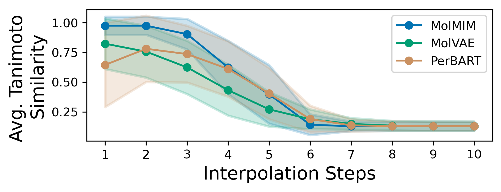
Figure 2: Average Tanimoto similarity (y-axis) between input and non-identical interpolated molecules (x-axis is interpolation step). Colored areas indicate standard deviation. MolMIM clusters similar molecules and has the smallest variance in early steps.

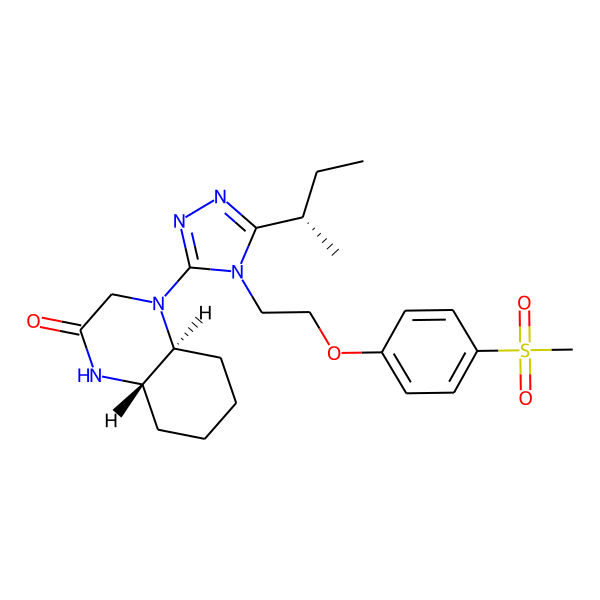
(a) Initial

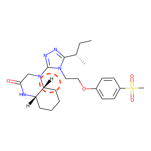
(b) Perturbed

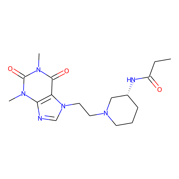
(c) Initial

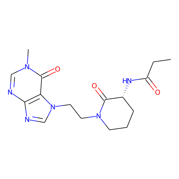
(d) Perturbed

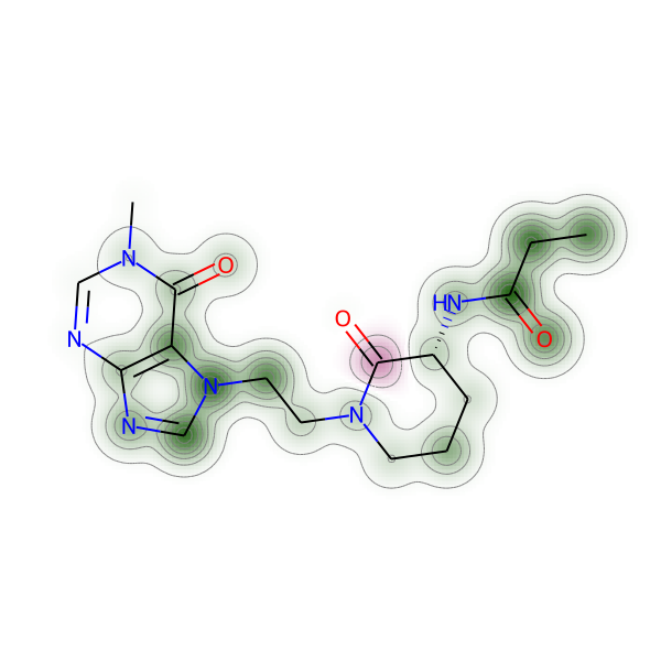
(e) Similarity Map

Figure 3: MolMIM’s fine-grained control over molecule generation. (a-b) Small perturbations lead to changes in chirality only (circled in dashed red). (c-d) Bigger changes allow the substitution of a single atom (red background in similarity map (e)). The similarity map depicts green background for chemically similar structures and red background for modified structures.

 

In addition to the ability to sample valid, unique, and novel molecules, we would like to train a model with a learned latent structure that will lend itself to the optimization of molecular properties. In the context of unsupervised learning, the structure can relate to the similarity of observations, or intrinsic properties of latent codes (e.g., smoothness). We hypothesize that a latent space where latent codes of similar molecules are clustered together will allow for fine-grained control while searching for molecules with target properties.

In what follows we explore the clustering of molecules in the latent space using pair-wise interpolations of 1,000 test set molecules. This allows us to better understand the qualitative differences in the spatial structures of the respective latent spaces of each model. An interpolation entails projecting two molecules onto the latent space by taking the latent codes to be the respective mean of the posterior for each molecule. Following the method used by Gómez-Bombarelli et al. (2018), we then linearly interpolate between the latent codes over 10 equidistant steps, and for each interpolated latent code we decode a corresponding molecule. We then compute the Morgan fingerprint (Rogers & Hahn, 2010) with 2048 bits and radius 2, resulting in a bit vector of hashed molecular features for each molecule. Finally, the average Tanimoto similarity (Rogers & Hahn, 2010) is calculated between the Morgan fingerprints of the initial and all non-identical interpolated molecules.

Fig. 2 shows that MolVAE’s smooth latent space results in a gradual similarity decline, whereas MolMIM contains regions of high similarity followed by a sharper decline. MolVAE and PerBART show lower average similarity for interpolation step 1. For MolVAE, it is due to poor reconstruction in the absence of noise. For PerBART, the less ordered structure of its latent space leads to a quick divergence when small amounts of noise are added.

In contrast, MolMIM maintains near perfect similarity for steps 1 and 2, while producing non-identical molecules. MolMIM also demonstrates a significantly lower variance in steps 1-3, making it a reliable sampler when considering similarity. This is an interesting result as MolMIM is not explicitly trained with Tanimoto similarity information. We conclude from Fig. 2 that the latent structure of MolMIM is clustered by meaningful chemical similarity.

Fig. 3(b) depicts qualitative examples of the fine-grained control supported by MolMIM. Fig. 3(b)(a-b) demonstrate how small perturbations can lead to minimal changes, such as inversions of a chiral center of a single molecule (circled in dashed red). Fig. 3(b)(c-e) depict more significant changes where the similarity map highlights in red a single-atom change. The ability to generate molecules of even more diversity is discussed next.

4.3 Small Molecule Optimization

In what follows we use CMA-ES (Hansen, 2006), a greedy, gradient-free (i.e., 0^th order optimization), evolutionary search algorithm that maximizes a black-box reward function for small molecule optimization. CMA-ES is often used as an optimization baseline (e.g., Yang et al. (2021)), and does not scale well to high-dimensional problems. We apply CMA-ES directly to the latent space to generate proposed latent solutions thus expanding on the sampling technique discussed in Sec. 4.1. These putative solutions are then greedily decoded to generate molecules. The molecules are the required inputs to the reward function, which is comprised of molecular property oracle functions. We chose CMA-ES as it is a simple algorithm and weak baseline for novel optimization methods thus allowing us to isolate the optimization success of MolMIM to its latent structure. We believe that using more powerful latent optimization techniques, such as RL, could further improve the results. We used TDC (Huang et al., 2021) oracle functions for all chemical property values in this section. Here we demonstrate how such a naive algorithm can deliver state-of-the-art results given an informative and clustered latent space.

4.3.1 Single Property Optimization

	QED (%)	Penalized logP
Task	$\delta=0.4$	$\delta=0.6$	$\delta=0.4$
JT-VAE	8.8	0.28 $\pm$ 0.79	1.03 $\pm$ 1.39
GCPN	9.4	0.79 $\pm$ 0.63	2.49 $\pm$ 1.30
MolDQN	-	1.86 $\pm$ 1.21	3.37 $\pm$ 1.62
MMPA	32.9	-	-
VSeq2Seq	58.5	2.33 $\pm$ 1.17	3.37 $\pm$ 1.75
VJTNN+GAN	60.6	-	-
VJTNN	-	2.33 $\pm$ 1.24	3.55 $\pm$ 1.67
MoFlow	-	2.10 $\pm$ 2.86	4.71 $\pm$ 4.55
GA	-	3.44 $\pm$ 1.09	5.93 $\pm$ 1.41
AtomG2G	73.6	-	-
HierG2G	76.9	-	-
DESMILES	77.8	-	-
QMO	92.8	3.73 $\pm$ 2.85	7.71 $\pm$ 5.65
MolGrow	-	4.06 $\pm$ 5.61	8.34 $\pm$ 6.85
GraphAF	-	4.98 $\pm$ 6.49	8.21 $\pm$ 6.51
GraphDF	-	4.51 $\pm$ 5.80	9.19 $\pm$ 6.43
CDGS	-	5.10 $\pm$ 5.80	9.56 $\pm$ 6.33
FaST	-	8.98 $\pm$ 6.31	18.09 $\pm$ 8.72
MolMIM	94.6	7.60 $\pm$ 23.62	28.45 $\pm$ 54.67
MolMIM†		4.57 $\pm$ 3.87	9.44 $\pm$ 4.12

Table 2: QED and penalized logP optimization under minimal Tanimoto similarity constraint $\delta$. QED results show success percentage and penalized logP show the mean and standard deviation of the improvement in value. †  limits logP solutions to improvement $\leq$ 20. Bottom models are developed herein. For logP, 97.25% and 79.13% of the molecules saw an increase in score for $\delta\in{0.4,0.6}$ respectively, 100% were within the target $\delta$, and 0% saw a decrease in score.

In what follows we explore the optimization of a single chemical property under a Tanimoto similarity constraint $\delta$, which limits the allowed distance from an input molecule. Specifically, we target Quantitative Estimate of Drug-likeness (QED, Bickerton et al. (2012)) and penalized logP (Jin et al., 2018).

We use 800 molecules with QED $\in[0.7,0.8]$ (Jin et al., 2019b), and 800 molecules with low penalized logP scores (Jin et al., 2018) as the starting points for our respective optimizations. For the QED task, the success rate is defined as the percentage of generated molecules with QED $\geq 0.9$ while maintaining at least a $\delta=0.4$ Tanimoto similarity to the respective input (Jin et al., 2019b). For the penalized logP task, we report the mean and standard deviation of penalized logP improvement under a similarity constraint for $\delta\in\{0.4,0.6\}$ (Jin et al., 2018). We provide the reward functions and additional information in Appendix A.3.

In both experiments, we follow a query budget of 50,000 oracle calls per input molecule, following Hoffman et al. (2022). We have found that dividing each optimization into 50 restarts with 1,000 CMA-ES iterations, and a population size of 20 to yield the best results. We omit MegaMolBART from the next experiments since it is unclear how to utilize CMA-ES in a variable-size representation.

Table 2 shows that MolMIM yields new state-of-the-art results in both QED and penalized logP optimization tasks. We also point the reader to the large value of the standard deviation for the logP experiment, in which MolMIM exploits a known flaw in the logP oracle function where generating molecules with long saturated carbon chains yield high logP values (Renz et al., 2019).

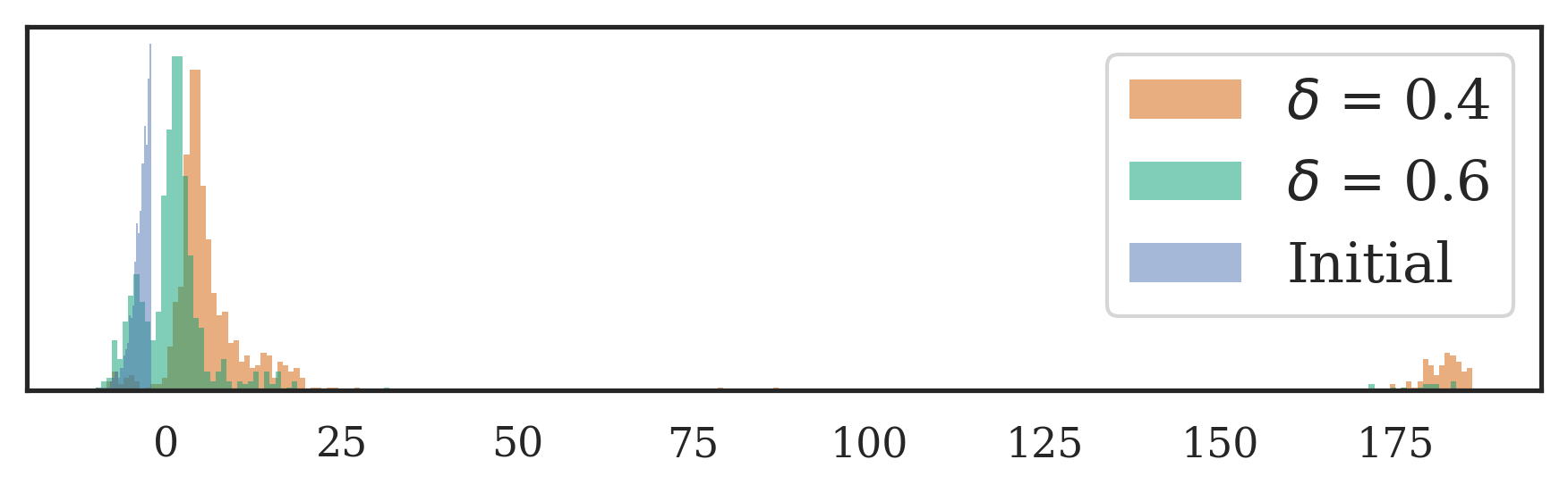
Figure 4: Penalized logP distribution of initial molecules (blue) and optimized molecules under increasingly stringent Tanimoto similarity constraints of 0.4 and 0.6 (orange and green, respectively). The right-hand side mode represents a common bias in the pen. logP oracle function.

Fig. 4 clearly shows a bimodal distribution with the right-hand side mode depicting the logP exploitation described above. As these saturated molecules are not useful in practice (Renz et al., 2019), we also provide results of MolMIM† in Table 2. Here we limit the maximal penalized logP improvement to 20 during the optimization procedure, removing the problematic mode. By doing so we obtain a significantly smaller standard deviation while still maintaining a high mean value and 100% success rate. We stress that the structure of MolMIM’s latent space allows a simple CMA-ES to outperform CDGS which relied on a complex diffusion procedure and ODE solvers. Only FaST and MolMIM† can achieve a standard deviation less than its mean for the more difficult similarity constraint $\delta=0.6$.

As a final single property experiment, we point the reader to the Appendix A.5 Table. 4 where we use CMA-ES with a limited iteration budget to optimize over each latent space. MolMIM consistently provides superior results over all other models, including CDDD, especially at the lower limit of 100 iterations (roughly 2x performance increase).

4.3.2 Multi-Objective Property Optimization

	GSK3$\beta$ + JNK3 + QED + SA
Model	Success (%)	Novelty (%)	Diversity
JT-VAE	1.3	-	-
GVAE-RL	2.1	-	-
GCPN	4.0	-	-
REINVENT	47.9	-	-
RationaleRL	74.8	56.1	0.621
MARS	92.3	82.4	0.719
JANUS	100	32.6	.821
FaST	100	100	0.716
MolMIM (R)	97.5	71.1	0.791
MolMIM (A)	96.6	63.3	0.807
MolMIM (E)	98.3	55.1	0.767
MolMIM (E)†	99.2	54.8	0.772

Table 3: Multi-objective molecule optimization. (R) random initialization, (A) promising precursor initialization, (E) initialization with exemplars. †  results are based on additional restarts. Bottom models are developed herein.

Due to the fact that the unbounded optimization of penalized logP contradicts Lipinski’s rule of 5 (Lipinski et al., 1997), we chose a more challenging setting that better represents the complexity of real-world drug discovery (Coley et al., 2020; Chen et al., 2021). The task is defined over multiple objectives, where a randomly chosen molecule is jointly optimized for $\text{QED}\geq 0.6$, $\text{SA}\leq 4.0$, $\text{JNK3}\geq 0.5$, and $\text{GSK3}\beta\geq 0.5$. We follow the same procedure and model usage as defined by Jin et al. (2020) for predicting inhibition of JNK3 and GSK3$\beta$.

We consider three variants of initial molecule selection: (R) random start - 2,000 initial molecules are randomly sampled from the ZINC-15 test set; (A) approximate start - 551 initial molecules that satisfy all three conditions $\text{QED}\in[0.25,0.4),\text{JNK3}\in[0.25,0.35),\text{GSK3}\beta\in[0.25,0.35)$; (E) exemplar-based - 741 initial molecules that already satisfy the required success conditions. In the case of (E), we also force the optimized molecule to have at most 0.4 Tanimoto similarity to the initial molecule. The multi-property experiments entailed 28 restarts of 1500 iterations with a CMA-ES population size of 20. We provide the reward functions in Appendix A.3.

Table 3 shows the results measured by success rate, novelty, and diversity, as defined by Jin et al. (2020). Here, novelty is the percentage of generated molecules with Tanimoto similarity less than 0.4 compared to the nearest neighbor in the ChEMBL training set (Olivecrona et al., 2017). Diversity is defined as the pairwise Tanimoto similarity over Morgan fingerprints between all generated molecules $1-\frac{2}{n(n-1)}\sum_{{\bm{x}}\neq{\bm{x}}^{\prime}}TanSim({\bm{x}},{\bm{x}}^{\prime})$ where ${\bm{x}}$ is sampled without replacement.

Compared to JANUS, a genetic algorithm, MolMIM achieves competitive success rate and diversity while significantly improving novelty . MolMIM also achieves better diversity than FaST a recent molecular fragment-based optimization method that uses a novelty/diversity-aware RL policy. We note that MolMIM achieves competitive results without RL or other complex optimization methods and can later be combined with such in future research.

We also present in Table 3 results for MolMIM (E)†, where we launched additional restarts, reaching 49 in total. In such a case we present a very high success rate at the expense of novelty. We added MolMIM (E) to mimic more realistic drug development where we generate a new molecular structure while maintaining the desired properties. MolMIM (A) targets drug development use cases where, starting from a promising precursor, we want to generate a successful related molecule. MolMIM (E) increases the difficulty of the optimization task and now not only do we have to meet four property thresholds we also introduce a similarity maximum constraint.

In summary, we present three variants for multi-objective optimization. MolMIM demonstrates competitive results using a simple CMA-ES algorithm. We attribute the success of MolMIM to the informative and clustered latent space which proved to be useful for various optimization tasks.

5 Conclusions

In this paper, we present a novel probabilistic auto-encoder for small molecules called MolMIM. Trained with Mutual Information Machine (MIM) learning, the model learns an informative and clustered latent space and samples novel molecules with high probability. We utilize MolMIM to set multiple state-of-the-art results in single and multiple property optimization tasks through the incorporation of a simple search algorithm, CMA-ES. Importantly, any successful solution to the small molecule optimization problem can be applied to other biological modalities such as proteins, RNA, and DNA. Future research directions will include improvement of the latent space search, replacing CMAE-ES with a more informed search algorithm. In addition, the utilization of graphical molecular representations for training MolMIM might yield further improvement.

Appendix A Supplementary Material

A.1 Formal Model Definitions

Here we discuss the relation between auto-encoder (AE), VAE, and MIM. We explicitly show that MIM and VAE extends AE with a regularization term that promotes certain properties of the latent space, which are different for the two models.

A.1.1 Denoising Auto-encoder

MolMIM builds upon denoising auto-encoders (Goodfellow et al., 2016) where a corrupted input is encoded by an encoder into a latent code. The latent code is then used to reconstruct the original input by the decoder. More formally, we can describe auto-encoders (AE) in terms of encoding distribution $q_{{\bm{\theta}}}({\bm{z}}|{\bm{x}})$ and decoding distribution $p_{{\bm{\theta}}}({\bm{x}}|{\bm{z}})$, where we opt here for a probabilistic view. A deterministic encoder can be viewed as a Dirac delta function around the predicted mean. Given the encoder and decoder, the denoising AE (DAE) loss, per observation ${\bm{x}}$ can be expressed as,

$$\mathcal{L}_{\text{AE}}({\bm{\theta}})=\mathbb{E}_{{\bm{z}}\sim q_{{\bm{\theta}}}({\bm{z}}|\tilde{{\bm{x}}})}\left[\log p_{{\bm{\theta}}}({\bm{x}}|{\bm{z}})\right]$$ (4)

where ${\bm{x}}\in\mathcal{V}^{N}$ for vocabulary $\mathcal{V}$, $\tilde{{\bm{x}}}$ is some kind of corruption or augmentation of ${\bm{x}}$, ${\bm{z}}\in\mathbb{R}^{H}$, $H$ is the hidden dimensions, and ${\bm{\theta}}$ is the union of all learnable parameters. Here we include the identity function in the set of augmentations, where $\tilde{{\bm{x}}}\equiv{\bm{x}}$.

A.1.2 Bottleneck Architectures

A precursor to MolMIM is our baseline BART (Lewis et al., 2020) model referred to as MegaMolBART, with data augmentation identical to Chemformer (Irwin et al., 2022). BART is a transformer-based seq2seq model that learns a variable-size hidden representation $H=|\tilde{{\bm{x}}}|\times D$. That is, the dimension of the hidden representation is equal to the number of tokens in the encoder input times the embedding dimension. This makes sampling from the model especially challenging since the molecule length has to be sampled as well. In contrast, learning a fixed-size representation as typically done in denoising auto-encoders, where all molecules are mapped into the same space, makes sampling easier.

Thus, we propose to replace MegaMolBART’s Transformer encoder with a fixed-sized output Perceiver encoder (Jaegle et al., 2021). Perceiver is an attention-based architecture that utilizes cross-attention to project a variable input onto a fixed-size output. More formally, ${\bm{z}}\in\mathbb{R}^{H}$ for a pre-defined dimension $H$.

A.1.3 Latent Variable Models

A fixed-sized representation with a bottleneck architecture allows us to learn latent variable models (LVMs). A popular LVM is a Variational Auto-Encoder (VAE) and was introduced by Kingma & Welling (2014). VAE training expands on the typical denoising AE with the following loss per observations,

$$\mathcal{L}_{\text{VAE}}({\bm{\theta}})=\mathcal{L}_{\text{AE}}({\bm{\theta}})+\mathcal{D}_{\text{KL}}\left(q_{{\bm{\theta}}}({\bm{z}}|\tilde{{\bm{x}}})\,\|\,p_{{\bm{\theta}}}({\bm{z}})\right)$$ (5)

where $p_{{\bm{\theta}}}({\bm{z}})$ is the prior over the latent code, which is typically a Normal distribution as in our case. The KL divergence term encourages smoothness in the latent space. We define our posterior $q_{{\bm{\theta}}}$ to be a Gaussian with a diagonal covariance matrix. We sample ${\bm{z}}$ from the posterior using the reparametrization trick which leads to a low variance estimator of the gradient during training.

A main caveat of VAE is a phenomenon called posterior collapse where the learned encoding distribution is closely matching the prior, and the latent codes carry little information (Razavi et al., 2019). Posterior collapse leads to poor reconstruction accuracy, where the learned model performs well as a sampler, but allows little control over the generated molecule.

In contrast to VAE, MIM learning entails minimizing the following loss per observation

$$\mathcal{L}_{\text{MIM}}({\bm{\theta}})=\mathcal{L}_{\text{AE}}({\bm{\theta}})+\mathbb{E}_{q_{{\bm{\theta}}}}\left[\log\big{(}p_{{\bm{\theta}}}({\bm{z}})q_{{\bm{\theta}}}({\bm{z}}|\tilde{{\bm{x}}})q_{{\bm{\theta}}}({\bm{x}})\big{)}\right]$$ (6)

which promotes high mutual information between ${\bm{z}}$ and ${\bm{x}}$, and low marginal entropy in ${\bm{z}}$ (i.e., clustered representation). As discussed in Sec. 2, MolMIM was designed in response to the aforementioned flaws of variable-length transformer models and VAEs. To test our novel combination of bottleneck architecture and learning framework we compare MolMIM to MolVAE, and PerBART, which use the same Perceiver bottleneck architecture and general training procedure.

We note that the PerBART uses the same learning as a regular BART, which does not explicitly promotes any structure in the learned latent space. We show empirically that BART learns a latent space with “holes”, where sampling from a “hole” results in an invalid molecule. PerBART was specifically created to exemplify how the added latent regularization of MolMIM and MolVAE promotes structure in the latent space. Doing so allows a greater understanding of how both the addition of a bottleneck as well as the form of latent regularization impact generative molecular tasks in different ways.

A.2 Training Details

Dataset: All models were trained using a tranche of the ZINC-15 dataset (Sterling & Irwin, 2015), labeled as reactive and annotated, with molecular weight $\leq$ 500Da and logP $\leq$ 5. Of these molecules, 730M were selected at random and split into training, testing, and validation sets, with 723M molecules in the training set. We note that we do not explore the effect of model size, hyperparameters, and data on the models. Instead, we train all models on the same data using the same hyperparameters, focusing on the effect of the learning framework and the fixed-size bottleneck. For comparison, Chemformer was trained on 100M molecules from ZINC-15 (Sterling & Irwin, 2015) – 20X the size of the dataset used to train CDDD (72M from ZINC-15 and PubChem (Kim et al., 2018)). MoLFormer-XL was trained on 1.1 billion molecules from the PubChem and ZINC datasets.

Data augmentation: Following Irwin et al. (2022), we used two augmentation methods: masking, and SMILES enumeration (Weininger, 1988). Masking is as described for the BART MLM denoising objective, with 10% of the tokens being masked, and was only used during the training of MegaMolBART. In addition, MegaMolBART, PerBART, and MolVAE used SMILES enumeration where the encoder and decoder received different valid permutations of the input SMILES string. MolMIM was the only model to see an increase in performance when both the encoder and decoder received the same input SMILES permutation, simplifying the training procedure.

Model details: We implemented all models with NeMo Megatron toolkit (Kuchaiev et al., 2019). We used a RegEx tokenizer with 523 tokens (Bird et al., 2009). All models had 6 layers in the encoder and 6 layers in the decoder, with a hidden size of 512, 8 attention heads, and a feed-forward dimension of 2048. The Perceiver-based models also required defining K, the hidden length, which relates to the hidden dimension by $H=K\times D$ where $H$ is the total hidden dimension, and $D$ is the model dimension (Fig. 1). MegaMolBART had $58.9M$ parameters, PerBART had $64.6M$, and MolVAE and MolMIM had $65.2M$. We used greedy decoding in all experiments. We note that we trained MolVAE using the loss of $\beta$-VAE (Higgins et al., 2017) where we scaled the KL divergence term with $\beta=\frac{1}{D}$ where $D$ is the hidden dimensions.

Optimization: We use ADAM optimizer (Kingma & Ba, 2015) with a learning rate of 1.0, betas of 0.9 and 0.999, weight decay of 0.0, and an epsilon value of 1.0e-8. We used Noam learning rate scheduler (Vaswani et al., 2017) with a warm-up ratio of 0.008, and a minimum learning rate of 1e-5. During training, we used a maximum sequence length of 512, dropout of 0.1, local batch size of 256, and global batch size of 16384. All models were trained for 1,000,000 steps with fp16 precision for 40 hours on 4 nodes with 16 GPU/node (Tesla V100 32GB). MolVAE was trained using $\beta$-VAE (Higgins et al., 2017) with $\beta=\frac{1}{H}$ where $H$ is the number of hidden dimensions. We have found this choice to provide a reasonable balance between the rate and distortion (see Alemi et al. (2018) for details). It is important to note that MolMIM does not require the same $\beta$ hyperparameter tuning as done for VAE.

A.3 Small Molecule Optimization

In this section, we formulate the reward functions that were used in the small molecule optimization part of the main body.

A.3.1 Single Property Optimization

Quantitative Estimate of Druglikeness (QED) is a simple rule-based molecular property that measures drug-likeliness (Bickerton et al., 2012). Penalized logP (Jin et al., 2018) is logP, which is the $\log_{10}$ of the octanol and water solute partition ratio and is a measure of hydrophobicity with larger values indicating increased hydrophobicity, minus the Synthetic Accessibility (SA) score (Ertl & Schuffenhauer, 2009).

Formally, we define the following reward functions for our CMA-ES optimization:

$$\mathcal{R}_{QED} =\min(\frac{QED}{0.9},1)+\min(\frac{TanSim}{0.4},1)$$ (7)

$$\mathcal{R}_{plogP} =\frac{plogP}{20}+\min(\frac{TanSim}{\delta},1)$$ (8)

where $TanSim$ is the Tanimoto similarity, $\delta$ is the value of the similarity constraint, and $QED,\ plogP$ are the corresponding properties. The loss scaling of each term was tuned manually over a few test runs.

A.3.2 Multi Property Property Optimization

JNK3 is the inhibition of c-Jun N-terminal kinase-3. GSK3$\beta$ is the inhibition of glycogen synthase kinase-3 beta.

Formally, we show the reward function below,

$$\mathcal{R}_{MP}^{R,A} =\frac{QED+GSK3\beta}{2}+\frac{SA}{40}+JNK3$$ (9)

$$\mathcal{R}_{MP}^{E} =\frac{1}{50}\mathcal{R}_{MP}^{R,A}+\min(1.0,\frac{1-TanSim}{1-0.4})$$ (10)

where $TanSim$ is the Tanimoto similarity, and $QED,\ SA,\ JNK3,\ GSK3\beta$ are the corresponding properties. The loss scaling of each term was tuned manually over a few test runs.

A.4 Finding Optimal Noise Scale for Top Models

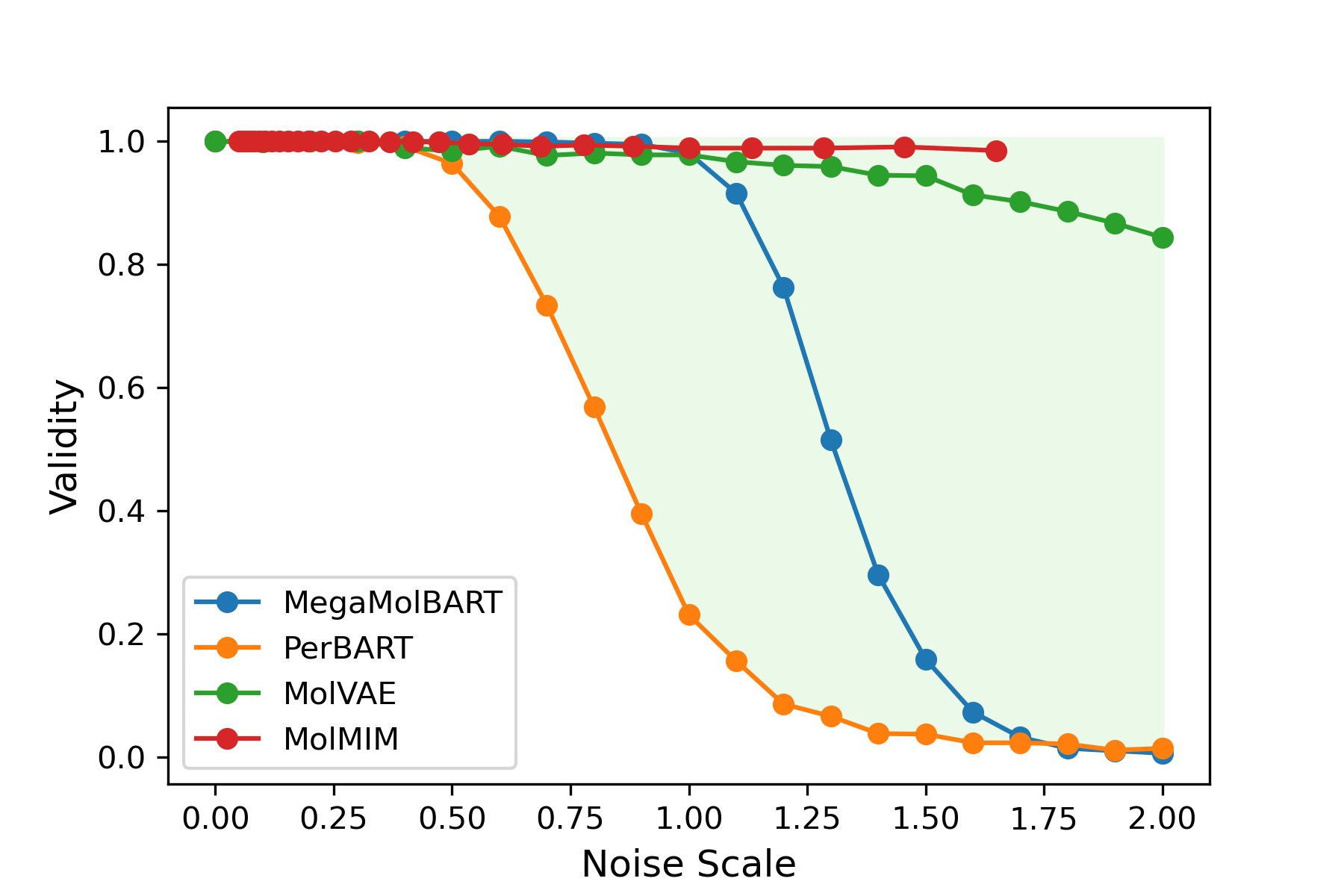
Figure 5: Validity as a function of noise scale. Note how latent variable models, MolVAE and MolMIM, are consistent while the others, MegaMolBART and PerBART, see a sharp decline at larger noise scales.

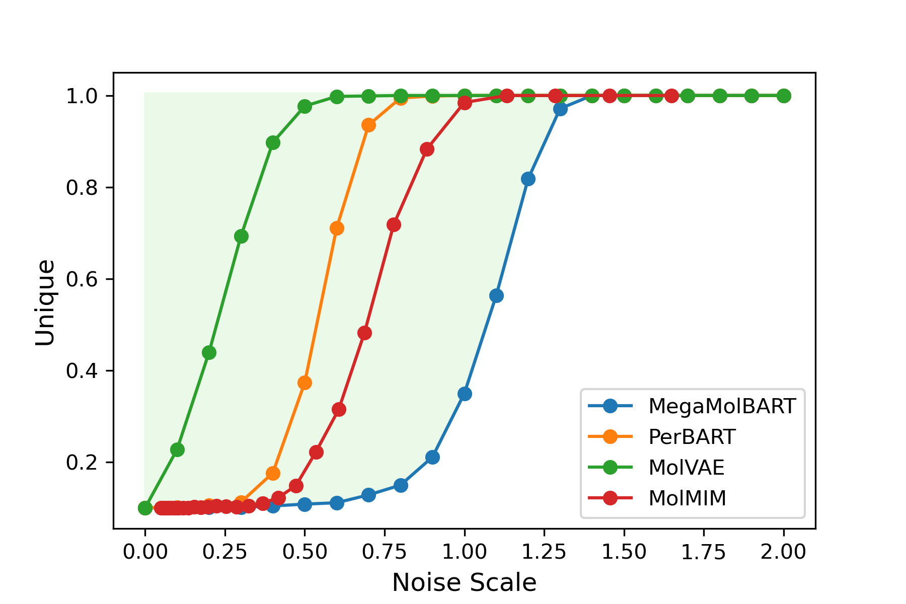
Figure 6: Uniqueness as a function of noise scale. Note MegaMolBART is a lower bound for the entire range of tested noise scales.

Figure 7: Non-Identicality as a function of noise scale. Note at a nose scale of 0, only MolVAE has a non zero non-identicality as a result of poor reconstruction (i.e., relates to posterior collapse).

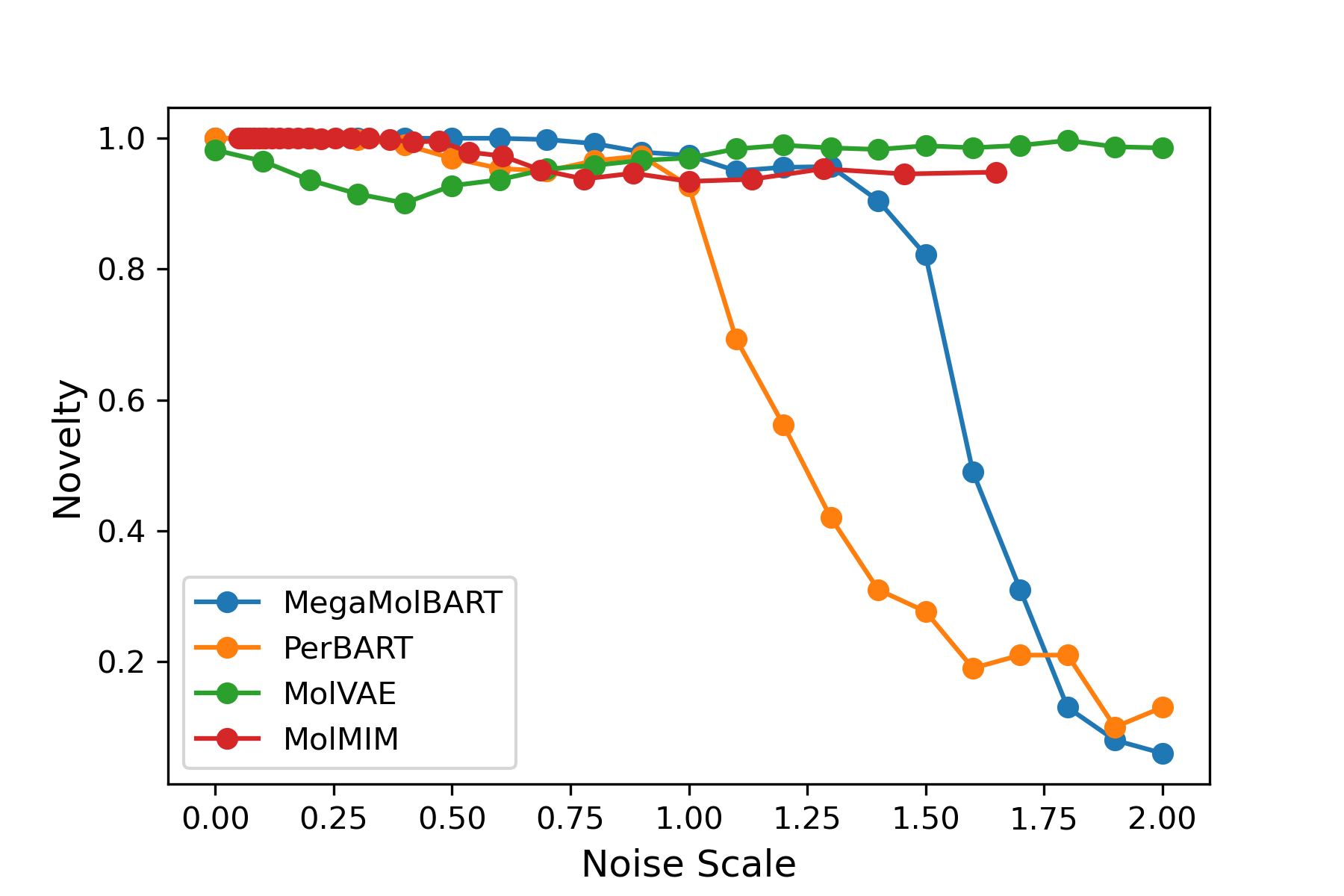
Figure 8: Novelty as a function of noise scale. Note how latent variable models, MolVAE and MolMIM, are consistent while the others, MegaMolBART and PerBART, see a sharp decline due to the increased validity issues at large noise scales.

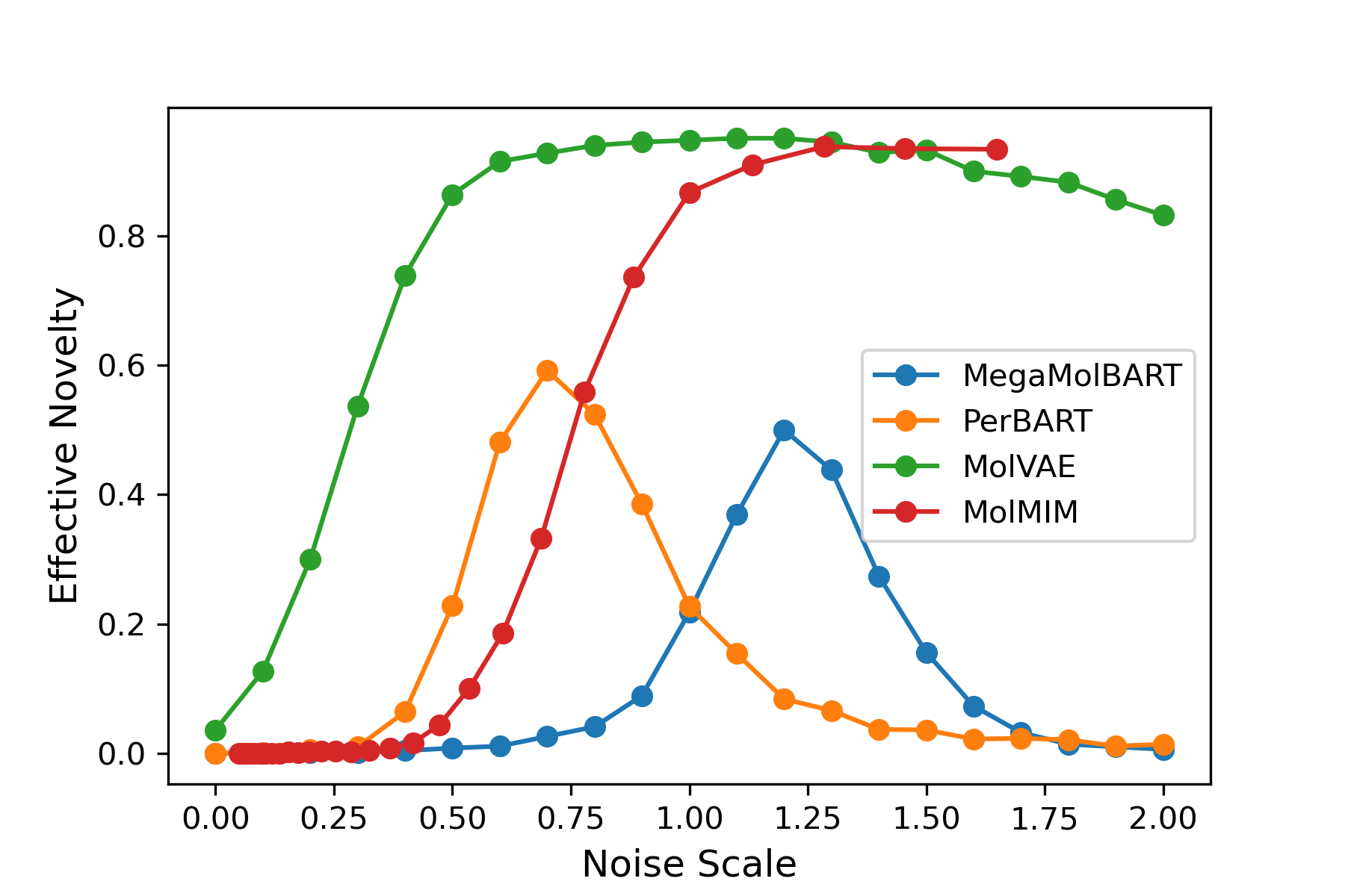
Figure 9: Effective Novelty as a function of noise scale. Note the non-latent variable models, MegaMolBART and PerBART, have a parabolic shape due to validity issues at large noise scales.

In this section, we show the results of the hyperparameter search for the optimal noise scale that maximizes effective novelty, per model. See Figs. 5, 6, 7, 8, 9. We omit here the search for the optimal hidden length $K$ per model, where we considered $K\in{1,2,4,8,16}$ for all models.

A.5 Compute Limited Single Property Optimization

	Success % of QED (iter)				Pen. logP  ($\bm{\delta=0.4}$)
Model	100	300	400	800	avg. $\Delta$	% ($\Delta>0$)
PerBART	2	2.12	-	-	2.6 ± 2.3	23
MolVAE	6.6	21.2	-	-	3.0 ± 2.8	40.6
MolMIM	37	58	66.8	70.5	4.2 ± 1.6	78
CDDD	16	38	51.0	70.2	2.1 ± 2.4	45

Table 4: Results based on compute limited to a single restart and specified number of iterations. Penalized logP uses 100 iterations. We see that MolMIM improves upon all tested methods in terms of success rate for QED, and average increase and improvement percentage for logP. Missing results are due to excessively long run times. Top models are developed herein.

As a final single property experiment, we explore the above tasks using significantly reduced query budgets, and only a single restart. We consider 100, 300, 400, and 800 iterations for the QED task, and 100 iterations for the penalized logP task. Table. 4 shows the results, where MolMIM consistently provides superior results over all other models, including CDDD, which is trained with chemical property information. It is important to mention that only CDDD exhibited the generation of invalid molecules during the optimization procedure. We note that the improved performance of both MolMIM and MolVAE, relative to PerBART demonstrates the importance of having a regularized latent space. We also point the reader to the significant difference between MolMIM and MolVAE, demonstrating the importance of the learned latent spaces.

A.6 Sampling Metrics

A.6.1 Sampling Metric Formulation

Here, we formulate the sampling metrics as described in the main body:

validity $$~{}=~{} \frac{|V|}{|G|}$$ (11)

uniqueness $$~{}=~{} \frac{|U|}{|V|}$$ (12)

novelty $$~{}=~{} \frac{|N|}{|U|}$$ (13)

non identicality $$~{}=~{} \frac{|\bar{I}|}{|V|}$$ (14)

effective novelty $$~{}=~{} \frac{|N\cap\bar{I}|}{|G|}$$ (15)

where

• $G$ is the set of all generated molecules

• $V$ is the subset of all valid molecules in $G$

• $U$ is the subset of all unique molecules in $V$

• $N$ is the subset of all novel molecules in $U$

• $\bar{I}$ is the subset of all non identical molecules in $V$

are the corresponding sets.

The design flaw in Eq. 13 is that $N$ is a subset of $U$ and therefore does not consider the total amount of generated molecules $G$. Effective novelty not only measures the percentage of useful molecules but it also provides a measurement for sampling efficiency as it is defined over all generated molecules in Eq. 15.

A.6.2 Visualizing Effective Novelty

Novelty is based on molecules that are not present in the training set. However, it does not discriminate against duplicates. In such a case, one might need to sample multiple times to achieve the desired quantity of novel molecules. For this reason, it can be convenient to have a single metric that describes the sampling efficiency of the model. As an example, imagine a model reconstructs the novel input molecule 50% of the time, and the other 50% of the time generates different molecules which are valid, novel, and unique. If such a model produces 10 samples, the novelty will be 100%, and the uniqueness will be 60%. If the objective is to generate 10 novel molecules, we will have to sample 20 times from this model, which is deceiving for a novelty of 100%. To address the above issue and in order to simplify the evaluation of the sampling quality of a model, we introduce two new metrics Non-Identicality and Effective Novelty. In the case of the example above, the effective novelty will be 50%.

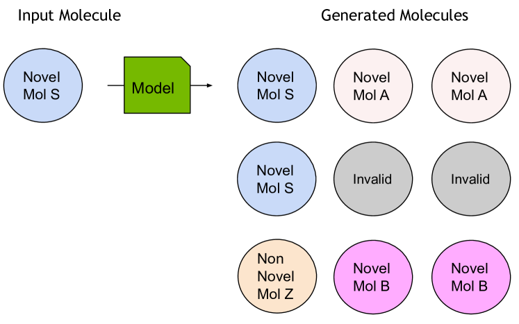
Figure 10: Given a novel input molecule S, we provide an example sampling output used in Figure. 11 to visualize all of the defined metrics Eq. 11 - 15

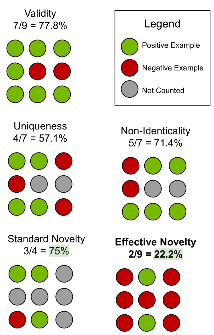
Figure 11: Here, we highlight the difference between novelty and effective novelty. For each metric, we mark the numerator (green), the denominator (green + red), and the irrelevant part(gray). The high novelty might still lead to low efficiency in sampling novel molecules.

We provide a depiction of effective novelty in Figs. 10-11 for further understandings..

References

- Alemi et al. (2018) Alexander Alemi, Ben Poole, Ian Fischer, Joshua Dillon, Rif A. Saurous, and Kevin Murphy. Fixing a broken ELBO. In Jennifer Dy and Andreas Krause (eds.), ICML, volume 80 of Proceedings of Machine Learning Research, pp. 159–168. PMLR, 10–15 Jul 2018.
- Bahdanau et al. (2015) Dzmitry Bahdanau, Kyung Hyun Cho, and Yoshua Bengio. Neural machine translation by jointly learning to align and translate. In ICLR, January 2015.
- Berenberg et al. (2022) Daniel Berenberg, Jae Hyeon Lee, Simon Kelow, Ji Won Park, Andrew Watkins, Vladimir Gligorijević, Richard Bonneau, Stephen Ra, and Kyunghyun Cho. Multi-segment preserving sampling for deep manifold sampler, 2022. URL https://arxiv.org/abs/2205.04259.
- Bickerton et al. (2012) G. Richard Bickerton, Gaia V. Paolini, Jérémy Besnard, Sorel Muresan, and Andrew L. Hopkins. Quantifying the chemical beauty of drugs. Nature Chemistry, 4(2):90–98, Feb 2012. ISSN 1755-4349.
- Bird et al. (2009) Steven Bird, Ewan Klein, and Edward Loper. Natural language processing with Python: analyzing text with the natural language toolkit. ” O’Reilly Media, Inc.”, 2009.
- Bowman et al. (2016) Samuel R. Bowman, Luke Vilnis, Oriol Vinyals, Andrew M. Dai, Rafal Józefowicz, and Samy Bengio. Generating sentences from a continuous space. In CoNLL, 2016.
- Brown et al. (2019) Nathan Brown, Marco Fiscato, Marwin H.S. Segler, and Alain C. Vaucher. Guacamol: Benchmarking models for de novo molecular design. Journal of Chemical Information and Modeling, 59(3):1096–1108, 2019.
- Chen et al. (2021) Benson Chen, Xiang Fu, Regina Barzilay, and Tommi S. Jaakkola. Fragment-based sequential translation for molecular optimization. In NeurIPS 2021 AI for Science Workshop, 2021. URL https://openreview.net/forum?id=E˙Slr0JVvuC.
- Chuai et al. (2018) Guohui Chuai, Hanhui Ma, Jifang Yan, Ming Chen, Nanfang Hong, Dongyu Xue, Chi Zhou, Chenyu Zhu, Ke Chen, Bin Duan, Feng Gu, Sheng Qu, Deshuang Huang, Jia Wei, and Qi Liu. Deepcrispr: optimized crispr guide rna design by deep learning. Genome Biology, 19(1):80, Jun 2018. ISSN 1474-760X. doi: 10.1186/s13059-018-1459-4. URL https://doi.org/10.1186/s13059-018-1459-4.
- Coley et al. (2020) Connor W. Coley, Natalie S. Eyke, and Klavs F. Jensen. Autonomous discovery in the chemical sciences part ii: Outlook. Angewandte Chemie International Edition, 59(52):23414–23436, 2020.
- Dalke et al. (2018) Andrew Dalke, Jérôme Hert, and Christian Kramer. mmpdb: An open-source matched molecular pair platform for large multiproperty data sets. Journal of Chemical Information and Modeling, 58(5):902–910, 2018.
- Engkvist et al. (2021) Ola Engkvist, Josep Arús-Pous, Esben Jannik Bjerrum, and Hongming Chen. Chapter 13 molecular de novo design through deep generative models. In Artificial Intelligence in Drug Discovery, pp. 272–300. The Royal Society of Chemistry, 2021. ISBN 978-1-78801-547-9. doi: 10.1039/9781788016841-00272. URL http://dx.doi.org/10.1039/9781788016841-00272.
- Ertl & Schuffenhauer (2009) Peter Ertl and Ansgar Schuffenhauer. Estimation of synthetic accessibility score of drug-like molecules based on molecular complexity and fragment contributions. Journal of Cheminformatics, 1(1):8, Jun 2009. ISSN 1758-2946.
- Goodfellow et al. (2016) Ian Goodfellow, Yoshua Bengio, and Aaron Courville. Deep Learning. MIT Press, 2016. http://www.deeplearningbook.org.
- Gómez-Bombarelli et al. (2018) Rafael Gómez-Bombarelli, Jennifer N. Wei, David Duvenaud, José Miguel Hernández-Lobato, Benjamín Sánchez-Lengeling, Dennis Sheberla, Jorge Aguilera-Iparraguirre, Timothy D. Hirzel, Ryan P. Adams, and Alán Aspuru-Guzik. Automatic chemical design using a data-driven continuous representation of molecules. ACS Central Science, 4(2):268–276, 2018. doi: 10.1021/acscentsci.7b00572. URL https://doi.org/10.1021/acscentsci.7b00572. PMID: 29532027.
- Hansen (2006) Nikolaus Hansen. The cma evolution strategy: A comparing review, 2006.
- Higgins et al. (2017) Irina Higgins, Loic Matthey, Arka Pal, Christopher Burgess, Xavier Glorot, Matthew Botvinick, Shakir Mohamed, and Alexander Lerchner. beta-VAE: Learning basic visual concepts with a constrained variational framework. In ICLR, 2017.
- Hoffman et al. (2022) Samuel C. Hoffman, Vijil Chenthamarakshan, Kahini Wadhawan, Pin-Yu Chen, and Payel Das. Optimizing molecules using efficient queries from property evaluations. Nature Machine Intelligence, 4(1):21–31, Jan 2022. ISSN 2522-5839. doi: 10.1038/s42256-021-00422-y. URL https://doi.org/10.1038/s42256-021-00422-y.
- Huang et al. (2023) Han Huang, Leilei Sun, Bowen Du, and Weifeng Lv. Conditional diffusion based on discrete graph structures for molecular graph generation. ArXiv, abs/2301.00427, 2023.
- Huang et al. (2021) Kexin Huang, Tianfan Fu, Wenhao Gao, Yue Zhao, Yusuf Roohani, Jure Leskovec, Connor W Coley, Cao Xiao, Jimeng Sun, and Marinka Zitnik. Therapeutics data commons: Machine learning datasets and tasks for drug discovery and development. NeurIPS Datasets and Benchmarks, 2021.
- Irwin et al. (2022) Ross Irwin, Spyridon Dimitriadis, Jiazhen He, and Esben Jannik Bjerrum. Chemformer: a pre-trained transformer for computational chemistry. Machine Learning: Science and Technology, 3(1):015022, jan 2022. doi: 10.1088/2632-2153/ac3ffb. URL https://doi.org/10.1088/2632-2153/ac3ffb.
- Jaegle et al. (2021) Andrew Jaegle, Felix Gimeno, Andy Brock, Oriol Vinyals, Andrew Zisserman, and Joao Carreira. Perceiver: General perception with iterative attention. In Marina Meila and Tong Zhang (eds.), Proceedings of the 38th International Conference on Machine Learning, volume 139 of Proceedings of Machine Learning Research, pp. 4651–4664. PMLR, 18–24 Jul 2021. URL https://proceedings.mlr.press/v139/jaegle21a.html.
- Jin et al. (2018) Wengong Jin, Regina Barzilay, and Tommi Jaakkola. Junction tree variational autoencoder for molecular graph generation. In Jennifer Dy and Andreas Krause (eds.), ICML, volume 80 of Proceedings of Machine Learning Research, pp. 2323–2332. PMLR, 10–15 Jul 2018.
- Jin et al. (2019a) Wengong Jin, Regina Barzilay, and Tommi Jaakkola. Hierarchical graph-to-graph translation for molecules, 2019a. URL https://arxiv.org/abs/1907.11223.
- Jin et al. (2019b) Wengong Jin, Kevin Yang, Regina Barzilay, and Tommi Jaakkola. Learning multimodal graph-to-graph translation for molecule optimization. In ICLR, 2019b.
- Jin et al. (2020) Wengong Jin, Dr.Regina Barzilay, and Tommi Jaakkola. Multi-objective molecule generation using interpretable substructures. In Hal Daumé III and Aarti Singh (eds.), ICML, volume 119 of Proceedings of Machine Learning Research, pp. 4849–4859. PMLR, 13–18 Jul 2020.
- Kim et al. (2020) Hyunho Kim, Eunyoung Kim, Ingoo Lee, Bongsung Bae, Minsu Park, and Hojung Nam. Artificial intelligence in drug discovery: A comprehensive review of data-driven and machine learning approaches. Biotechnol. Bioprocess Eng., 25(6):895–930, 2020.
- Kim et al. (2018) Sunghwan Kim, Jie Chen, Tiejun Cheng, Asta Gindulyte, Jia He, Siqian He, Qingliang Li, Benjamin A Shoemaker, Paul A Thiessen, Bo Yu, Leonid Zaslavsky, Jian Zhang, and Evan E Bolton. PubChem 2019 update: improved access to chemical data. Nucleic Acids Research, 47(D1):D1102–D1109, 10 2018. ISSN 0305-1048. doi: 10.1093/nar/gky1033. URL https://doi.org/10.1093/nar/gky1033.
- Kingma & Ba (2015) Diederik P. Kingma and Jimmy Ba. Adam: A method for stochastic optimization. In Yoshua Bengio and Yann LeCun (eds.), ICLR, 2015.
- Kingma & Welling (2014) Diederik P. Kingma and Max Welling. Auto-encoding variational bayes. CoRR, abs/1312.6114, 2014.
- Kuchaiev et al. (2019) Oleksii Kuchaiev, Jason Li, Huyen Nguyen, Oleksii Hrinchuk, Ryan Leary, Boris Ginsburg, Samuel Kriman, Stanislav Beliaev, Vitaly Lavrukhin, Jack Cook, et al. Nemo: a toolkit for building ai applications using neural modules. arXiv preprint arXiv:1909.09577, 2019.
- Kuznetsov & Polykovskiy (2021) Maksim Kuznetsov and Daniil Polykovskiy. Molgrow: A graph normalizing flow for hierarchical molecular generation. Proceedings of the AAAI Conference on Artificial Intelligence, 35(9):8226–8234, May 2021. ISSN 2159-5399. doi: 10.1609/aaai.v35i9.17001. URL http://dx.doi.org/10.1609/aaai.v35i9.17001.
- Lewis et al. (2020) Mike Lewis, Yinhan Liu, Naman Goyal, Marjan Ghazvininejad, Abdelrahman Mohamed, Omer Levy, Veselin Stoyanov, and Luke Zettlemoyer. BART: Denoising sequence-to-sequence pre-training for natural language generation, translation, and comprehension. In ACL, pp. 7871–7880, Online, July 2020. Association for Computational Linguistics. doi: 10.18653/v1/2020.acl-main.703. URL https://aclanthology.org/2020.acl-main.703.
- Li et al. (2020) Ruizhe Li, Xutan Peng, Chenghua Lin, Wenge Rong, and Zhigang Chen. On the low-density latent regions of vae-based language models. In Luca Bertinetto, João F. Henriques, Samuel Albanie, Michela Paganini, and Gül Varol (eds.), NeurIPS Workshop on Pre-registration in Machine Learning, volume 148 of Proceedings of Machine Learning Research, pp. 343–357. PMLR, 11 Dec 2020.
- Lipinski et al. (1997) Christopher A. Lipinski, Franco Lombardo, Beryl W. Dominy, and Paul J. Feeney. Experimental and computational approaches to estimate solubility and permeability in drug discovery and development settings. Advanced Drug Delivery Reviews, 23(1):3–25, 1997. ISSN 0169-409X. doi: https://doi.org/10.1016/S0169-409X(96)00423-1. URL https://www.sciencedirect.com/science/article/pii/S0169409X96004231. In Vitro Models for Selection of Development Candidates.
- Livne et al. (2019) Micha Livne, Kevin Swersky, and David J. Fleet. MIM: Mutual Information Machine. arXiv e-prints, 2019.
- Livne et al. (2020) Micha Livne, Kevin Swersky, and David J. Fleet. Sentencemim: A latent variable language model, 2020. URL https://arxiv.org/abs/2003.02645.
- Luo et al. (2021) Youzhi Luo, Keqiang Yan, and Shuiwang Ji. Graphdf: A discrete flow model for molecular graph generation. In Marina Meila and Tong Zhang (eds.), ICML, volume 139 of Proceedings of Machine Learning Research, pp. 7192–7203. PMLR, 18–24 Jul 2021.
- Mahmood et al. (2021) Omar Mahmood, Elman Mansimov, Richard Bonneau, and Kyunghyun Cho. Masked graph modeling for molecule generation. Nature Communications, 12(1):3156, May 2021. ISSN 2041-1723.
- Maragakis et al. (2020) Paul Maragakis, Hunter Nisonoff, Brian Cole, and David E. Shaw. A deep-learning view of chemical space designed to facilitate drug discovery. Journal of Chemical Information and Modeling, 60(10):4487–4496, 2020.
- Nigam et al. (2020) AkshatKumar Nigam, Pascal Friederich, Mario Krenn, and Alan Aspuru-Guzik. Augmenting genetic algorithms with deep neural networks for exploring the chemical space. In ICLR, 2020.
- Nigam et al. (2022) AkshatKumar Nigam, Robert Pollice, and Alán Aspuru-Guzik. Parallel tempered genetic algorithm guided by deep neural networks for inverse molecular design. Digital Discovery, 1:390–404, 2022. doi: 10.1039/D2DD00003B. URL http://dx.doi.org/10.1039/D2DD00003B.
- NVIDIA (2021) NVIDIA, Jul 2021. URL https://github.com/NVIDIA/MegaMolBART.
- Olivecrona et al. (2017) Marcus Olivecrona, Thomas Blaschke, Ola Engkvist, and Hongming Chen. Molecular de-novo design through deep reinforcement learning. Journal of Cheminformatics, 9(1):48, Sep 2017. ISSN 1758-2946.
- Razavi et al. (2019) Ali Razavi, Aaron van den Oord, Ben Poole, and Oriol Vinyals. Preventing posterior collapse with delta-VAEs. In ICLR, 2019.
- Renz et al. (2019) Philipp Renz, Dries Van Rompaey, Jörg Kurt Wegner, Sepp Hochreiter, and Günter Klambauer. On failure modes in molecule generation and optimization. Drug Discovery Today: Technologies, 32-33:55–63, 2019. ISSN 1740-6749. doi: https://doi.org/10.1016/j.ddtec.2020.09.003.
- Rogers & Hahn (2010) David Rogers and Mathew Hahn. Extended-connectivity fingerprints. Journal of Chemical Information and Modeling, 50(5):742–754, 2010. doi: 10.1021/ci100050t. URL https://doi.org/10.1021/ci100050t. PMID: 20426451.
- Ross et al. (2022) Jerret Ross, Brian Belgodere, Vijil Chenthamarakshan, Inkit Padhi, Youssef Mroueh, and Payel Das. Large-scale chemical language representations capture molecular structure and properties. Nature Machine Intelligence, 4(12):1256–1264, 2022. doi: 10.1038/s42256-022-00580-7. URL https://doi.org/10.1038/s42256-022-00580-7.
- Rumelhart et al. (1986) David E. Rumelhart, Geoffrey E. Hinton, and Ronald J. Williams. Learning representations by back-propagating errors. Nature, 323:533–536, 1986.
- Shi et al. (2020) Chence Shi, Minkai Xu, Zhaocheng Zhu, Weinan Zhang, Ming Zhang, and Jian Tang. Graphaf: a flow-based autoregressive model for molecular graph generation, 2020.
- Sliwoski et al. (2014) Gregory Sliwoski, Sandeepkumar Kothiwale, Jens Meiler, and Edward W. Lowe. Computational methods in drug discovery. Pharmacological Reviews, 66(1):334–395, 2014. ISSN 0031-6997. doi: 10.1124/pr.112.007336.
- Sterling & Irwin (2015) Teague Sterling and John J. Irwin. Zinc 15 – ligand discovery for everyone. Journal of Chemical Information and Modeling, 55(11):2324–2337, 2015.
- Vamathevan et al. (2019) Jessica Vamathevan, Dominic Clark, Paul Czodrowski, Ian Dunham, Edgardo Ferran, George Lee, Bin Li, Anant Madabhushi, Parantu Shah, Michaela Spitzer, and Shanrong Zhao. Applications of machine learning in drug discovery and development. Nature Reviews Drug Discovery, 18(6):463–477, 2019.
- Vaswani et al. (2017) Ashish Vaswani, Noam Shazeer, Niki Parmar, Jakob Uszkoreit, Llion Jones, Aidan N Gomez, Ł ukasz Kaiser, and Illia Polosukhin. Attention is all you need. In I. Guyon, U. Von Luxburg, S. Bengio, H. Wallach, R. Fergus, S. Vishwanathan, and R. Garnett (eds.), Advances in Neural Information Processing Systems, volume 30. Curran Associates, Inc., 2017.
- Weininger (1988) David Weininger. Smiles, a chemical language and information system. 1. introduction to methodology and encoding rules. Journal of Chemical Information and Computer Sciences, 28(1):31–36, 1988.
- Winter et al. (2019) Robin Winter, Floriane Montanari, Frank Noé, and Djork-Arné Clevert. Learning continuous and data-driven molecular descriptors by translating equivalent chemical representations. Chemical Science, 10:1692–1701, 2019. doi: 10.1039/C8SC04175J. URL http://dx.doi.org/10.1039/C8SC04175J.
- Xie et al. (2021) Yutong Xie, Chence Shi, Hao Zhou, Yuwei Yang, Weinan Zhang, Yong Yu, and Lei Li. Mars: Markov molecular sampling for multi-objective drug discovery. In ICLR, 2021.
- Yang et al. (2021) Kevin Yang, Tianjun Zhang, Chris Cummins, Brandon Cui, Benoit Steiner, Linnan Wang, Joseph E. Gonzalez, Dan Klein, and Yuandong Tian. Learning space partitions for path planning. In A. Beygelzimer, Y. Dauphin, P. Liang, and J. Wortman Vaughan (eds.), NeurIPS, 2021.
- You et al. (2018) Jiaxuan You, Bowen Liu, Rex Ying, Vijay Pande, and Jure Leskovec. Graph convolutional policy network for goal-directed molecular graph generation. In NeurIPS, NIPS’18, pp. 6412–6422, Red Hook, NY, USA, 2018. Curran Associates Inc.
- Zang & Wang (2020) Chengxi Zang and Fei Wang. Moflow: An invertible flow model for generating molecular graphs. Proceedings of the 26th ACM SIGKDD International Conference on Knowledge Discovery and Data Mining, Aug 2020. doi: 10.1145/3394486.3403104. URL http://dx.doi.org/10.1145/3394486.3403104.
- Zhou et al. (2019) Zhenpeng Zhou, Steven Kearnes, Li Li, Richard N Zare, and Patrick Riley. Optimization of molecules via deep reinforcement learning. Sci Rep, 9(1):10752, July 2019.