SDSS-IV MaNGA: the chemical co-evolution of gas and stars in spiral galaxies

Abstract

We investigate archaeologically how the metallicity in both stellar and gaseous components of spiral galaxies of differing masses evolve with time, using data from the SDSS-IV MaNGA survey. For the stellar component, we can measure this evolution directly by decomposing the galaxy absorption-line spectra into populations of different ages and determining their metallicities. For the gaseous component, we can only measure the present-day metallicity directly from emission lines. However, there is a well-established relationship between gas metallicity, stellar mass and star formation rate which does not evolve significantly with redshift; since the latter two quantities can be determined directly for any epoch from the decomposition of the absorption-line spectra, we can use this relationship to infer the variation in gas metallicity over cosmic time. Comparison of present-day values derived in this way with those obtained directly from the emission lines confirms the validity of the method. Application of this approach to a sample of 1619 spiral galaxies reveals how the metallicity of these systems has changed over the last 10 billion years since cosmic noon. For lower-mass galaxies, both stellar and gaseous metallicity increase together, as one might expect in well-mixed fairly isolated systems. In higher-mass systems, the average stellar metallicity has not increased in step with the inferred gas metallicity, and actually decreases with time. Such disjoint behaviour is what one might expect if these more massive systems have accreted significant amounts of largely pristine gas over their lifetimes, and this material has not been well mixed into the galaxies.

1 Introduction

Measuring the levels of heavy elements within galaxies over time is fundamental in order to fully understand their evolution. Typically, the chemical composition of galaxies is quantified by determining the levels of elements heavier than helium – the “metallicities” – of the stars and gas within these galaxies. Recent reviews by Kewley et al. (2019) and Maiolino & Mannucci (2019) comprehensively discuss galactic gas metallicities, and Madau & Dickinson (2014) and Maiolino & Mannucci (2019) review metallicities of the stellar populations within galaxies. While most studies of chemical evolution tend to focus on gas and stellar metallicities separately, these quantities can – and should – be treated on equal footing, since the stars whose metallicities we measure form from the same gas we are also interested in studying. Previous authors, such as Lian et al. (2018a); Lian et al. (2018b), and Yates et al. (2021), have found success in modelling the metallicities of the gas and the stars within galaxies in tandem. The results from this paper will aid the efforts of such authors by providing observational evidence to feed into these models.

Metallicities are known to evolve with cosmic time. However, the precise evolution of the metal content of both the gas and the stellar populations within galaxies is still not fully understood. Since metallicities are closely associated with other fundamental galaxy properties such as star formation rates (SFRs) and stellar masses (e.g. Mannucci et al., 2010; Yates et al., 2012; Curti et al., 2020), this is a crucial problem for astronomy to solve. Consequently, the evolution of metallicities back to the point at which galactic SFRs were at their most prodigious is of particular interest. This epoch, known as “cosmic noon”, occurred at a redshift of $z\sim 1.5$ (Madau et al., 1998; Madau & Dickinson, 2014). It is thus especially important to investigate how metallicities have evolved since cosmic noon to build a robust model of galaxy evolution.

In recent years, stellar metallicity histories have been determined thanks to observations of low-redshift, spatially resolved galaxies made by integral field unit (IFU) surveys such as the Mapping Nearby Galaxies at Apache Point Observatory (MaNGA; Bundy et al., 2015) survey; the Calar Alto Legacy Integral Field Area (CALIFA; Sánchez et al., 2012) survey; and the Sydney-AAO (Australian Astronomical Observatory) Multi-object Integral field spectrograph (SAMI; Croom et al., 2012) galaxy survey. For example, Peterken et al. (2019, 2020), Camps-Fariña et al. (2021, 2022), and Fraser-McKelvie et al. (2022) estimate spatially resolved stellar metallicity histories by excavating the fossil records of nearby MaNGA, CALIFA, and SAMI galaxies respectively. Spectral fitting methods, such as those employed by these authors, allow us to track the evolution of the average stellar metallicity with time within individual galaxies. This evolution can be yet further constrained when such methods are used in conjunction with direct observations of average stellar metallicities in higher-redshift galaxies (see, for instance, Onodera et al., 2015; Sanders et al., 2021; and Beverage et al., 2021).

By contrast, determining the gas metallicity histories within galaxies has previously proved elusive. The gas metallicity of a given galaxy can be estimated at the time at which the light was emitted by measuring certain emission lines in the galactic spectra, but it is not possible to track the evolution of these emission lines back over cosmic time. Nevertheless, the desire to do so is well-motivated, as work by Vale Asari et al. (2007) demonstrates. From their analysis of the star formation histories (SFHs) of over 80 000 galaxies, these authors found that galaxies with lower mean gas metallicities evolved more slowly than metal-rich galaxies.

It is, of course, possible to model the gas metallicity histories of galaxies through the use of simulations, as work by authors such as Fu et al. (2012), Somerville et al. (2015) and Yates et al. (2021) demonstrates. Observationally, however, the evolution of the gas metallicity has traditionally been estimated by observing galaxies at increasing redshift (see, for example, work by Troncoso et al., 2014; Wuyts et al., 2014; and Kashino et al., 2017). Unfortunately, this approach provides us only with snapshots of the chemical evolution of galaxies; furthermore, the quality of such snapshots diminishes with the redshift at which they are obtained. In theory, it should be possible to track the complete evolution histories of the gas metallicity in low-redshift, spatially resolved galaxies, just as is done for the average stellar metallicity. However, the wealth of observational information from IFU surveys such as MaNGA has not yet been fully exploited to determine the fossil records of the gas metallicities, as has been so successfully done for the stars which formed from this same gas.

Fortunately, gas metallicities are closely linked to other physical properties of galaxies. In particular, star-forming galaxies with higher stellar masses exhibit higher SFRs (e.g. Brinchmann et al., 2004; Noeske et al., 2007; Whitaker et al., 2012; Greener et al., 2020). This correlation is often called the “star formation main sequence” (SFMS). More massive galaxies also tend to have higher gas metallicities – a correlation often referred to as the “mass–gas metallicity relation” ($\rm MZ_{g}R$; e.g. Tremonti et al., 2004; Mannucci et al., 2010; Zahid et al., 2013a; Maiolino & Mannucci, 2019). Moreover, and perhaps unsurprisingly, authors such as Mannucci et al. (2010), Lara-López et al. (2010), Yates et al. (2012), and Curti et al. (2020) have demonstrated that there exists a more fundamental relation between stellar mass, gas metallicity, and SFR. In essence, these authors find that gas metallicity exhibits a very tight relationship with both stellar mass and SFR. This relationship is generally referred to as the fundamental metallicity relation (FMR; see, for instance, Figure 2 of Mannucci et al., 2010). Since the FMR does not evolve with redshift out to at least $z\sim 2.5$ (Mannucci et al., 2010; Sanders et al., 2021), it is therefore possible to infer the gas metallicity at earlier cosmic times from quantities that are derivable from spectral fitting – namely, stellar mass and SFR as a function of redshift.

It should be noted that the FMR is under debate, with certain authors questioning the validity of such a relation (see, for instance, Kashino et al., 2016; Telford et al., 2016; and Cresci et al., 2019). In this paper, we assume the existence of such an FMR, in line with various of its proponents, including Mannucci et al. (2010), Lara-López et al. (2010), Yates et al. (2012), Sanders et al. (2018, 2021), and Curti et al. (2020). An extensive review of the FMR – and its origin – is given by Maiolino & Mannucci (2019).

This process of spectral fitting (i.e. decomposing the integrated galaxy spectrum into stellar population spectra of single ages and stellar metallicities) brings us into dangerous territory, and due care must be taken during the procedure. We have to ensure that the spectra are reliably decomposed into the full two-dimensional stellar metallicity–age plane of the single stellar population (SSP) templates. We must perform checks to ensure that this spectral decomposition can be done safely, after which we can confidently proceed with our analysis of the stellar masses and SFHs produced as a result of the procedure.

In this paper, we infer via galactic archaeology the evolution of both the gas and stellar metallicity over cosmic time for a well-defined sample of galaxies in the present-day Universe that have been observed by the MaNGA survey. These quantities are calculated for the same galaxies both at the present day and at a redshift of $z\sim 1.4$. The gas metallicity histories of the galaxies are determined by using the FMR of Mannucci et al. (2010). Giving equal consideration to both the gas and the stars within the galaxies allows us to probe the redshift evolution of their gas and stellar metallicities simultaneously back to the epoch of cosmic noon.

The paper is structured as follows. In Section 2 we outline technical details of the MaNGA survey and our sample selection. We explain how stellar and gas metallicities are determined – and also describe the various checks and tests we perform on the SSP templates employed in this work – in Section 3. The results of this paper are presented and discussed in Section 4, and finally Section 5 summarises our conclusions. In this work, we employ a Chabrier (2003) initial mass function (IMF), and we assume a $\rm\Lambda CDM$ cosmology with $\Omega_{M}=0.3$, $\Omega_{\Lambda}=0.7$, and $H_{0}=70\>\rm km\ s^{-1}\ Mpc^{-1}$.

2 Data and Analysis

2.1 MaNGA

MaNGA (Bundy et al., 2015) is part of the fourth generation of the Sloan Digital Sky Survey (SDSS-IV; Blanton et al., 2017), and has now completed spectroscopic observations for over 10 000 nearby galaxies (Yan et al., 2016b; Wake et al., 2017). Hexagonal IFU fibre bundles (Law et al., 2015) are connected to a spectrograph (Smee et al., 2013; Drory et al., 2015), which in turn is mounted on the $2.5\,{\rm m}$ telescope at Apache Point Observatory (Gunn et al., 2006). MaNGA acquires spectra for each galaxy to a distance of at least 1.5 effective radii, meaning that most of the light from the observed galaxies is captured. The wavelength range of MaNGA is $3600-10300~{}$\mathrm{\text{Å}}$$, and it has a spectral resolution of $R\sim 2000$ (Bundy et al., 2015). The Data Reduction Pipeline (DRP; Law et al., 2016) reduces and calibrates the raw data observed by MaNGA (Yan et al., 2016a), and the Data Analysis Pipeline (DAP; Westfall et al., 2019; Belfiore et al., 2019a) subsequently further processes these data to produce maps detailing the physical properties of each galaxy.

2.2 Sample Selection

In order to select a representative sample of spiral galaxies, we make use of classifications provided by the citizen science project Galaxy Zoo 2 (GZ2; Willett et al., 2013). The process that we follow is essentially identical to that described in Peterken et al. (2020) and Greener et al. (2021), except that we exploit data from the most recent eleventh (and final) MaNGA Product Launch (MPL-11). For a more detailed discussion of the method adopted here, we refer the reader to Willett et al. (2013) and Hart et al. (2016).

GZ2 classifications are available for a total of 9315 MPL-11 galaxies. The first step is to remove from this sample 81 galaxies which are obscured by a star or other artifact. To ensure we are only selecting spiral galaxies, we choose only those for which $>43\%$ of $N\geq 20$ respondents observed either spiral features or a disk in the galaxy (as recommended by Willett et al., 2013). This cut reduces the sample to 6727 candidates who may be spiral galaxies. Since we wish our sample to be comprised of unequivocally spiral galaxies, we also want to select only those that are oriented reasonably face-on. In addition to requiring that $>80\%$ of $N\geq 20$ respondents determine that each galaxy is not edge-on (Willett et al., 2013), we also select only those galaxies which have a photometric axis ratio of $\frac{b}{a}\geq 0.5$ (corresponding to an inclination of $i\geq$$$). This constraint is somewhat stricter than that proposed by Hart et al. (2017), and further reduces the sample size to reasonably face-on 2081 spiral galaxies. Finally, we reject any galaxies that were flagged for poor data quality by the DRP or had for any reason failed to produce the necessary DAP data sets. This leaves a final sample comprised of 1619 reasonably face-on spiral galaxies that are fit for analysis.

3 Metallicities

The chemical compositions of both the stellar populations as well as the gaseous interstellar medium (ISM) within the sample galaxies are considered in this paper. In this section, we detail the processes by which the metallicities of both the stars and the gas are measured.

3.1 Stellar Metallicities

The average stellar metallicities of the sample galaxies are calculated using the full-spectrum stellar population fitting code STARLIGHT (Cid Fernandes et al., 2005). The STARLIGHT fitting process is very similar to that implemented by Greener et al. (2020, 2021), and is fully detailed by Peterken et al. (2020, including their Appendix A). This fitting process used in this work has already been extensively tested by these authors. The main steps relevant to this work are described below.

Each of the MaNGA spectra are fitted using a linear combination of SSP templates from the E-MILES library of Vazdekis et al. (2016), which in turn is based on the earlier MILES library of Vazdekis et al. (2010). No binning of neighbouring spaxels is done, since we wish to fully retain all spatial information. During the fitting procedure, we adopt a Chabrier (2003) IMF, and the “Padova” isochrones of Girardi et al. (2000). The E-MILES templates constitute nine ages $(\log(\rm age/yr)=7.85,\>8.15,\>8.45,\>8.75,\>9.05,\>9.35,\>9.65,\>9.95,\>10.25)$ and six stellar metallicities $([\rm M/H]_{*}=-1.71,\>-1.31,\>-0.71,\>-0.40,\>+0.00,\allowbreak\>+0.22)$. To reproduce younger stellar populations, we include an additional six ages $(\log(\rm age/yr)=6.8,\>6.9,\>7.0,\allowbreak\>7.2,\>7.4,\>7.6)$ and two stellar metallicities $([\rm M/H]_{*}=-0.41,\>+0.00)$ from the templates of Asa’d et al. (2017). These younger templates are produced in the same way as the E-MILES templates, except the (very similar) isochrones of Bertelli et al. (1994) are used. Following the advice of Ge et al. (2018) and Cid Fernandes (2018), we run STARLIGHT in a configuration which prioritises robustness over computation times.

As Peterken et al. (2020) recommend, we do not use stellar metallicities at ages younger than $10^{7.6}\>\rm yr$ for any subsequent analysis, due to uncertainties in the derived SFHs of such populations (see also Cid Fernandes & González Delgado, 2010). These uncertainties are likely related to the “UV upturn” produced by planetary nebulae in old stellar populations (see Yi, 2008 for a review of this phenomenon). Furthermore, at ages younger than $10^{7.6}\>\rm yr$, the calculated stellar metallicities also become increasingly unreliable; young, metal-poor stars are rare, and thus it is difficult to create accurate SSP templates for such populations. Moreover, the optical spectra of very hot type O stars do not have significant metal absorption lines, and thus provide poor stellar metallicity diagnostics. We do, however, include in our analysis the SSP templates at this threshold age of $10^{7.6}\>\rm yr$. We do not use stellar metallicities in the age bin at $10^{10.25}\>\rm yr$, since this is older than the age of the Universe. As such, it makes no physical sense to retain this age bin for our analysis.

The STARLIGHT fitting process generates a set of weights which encode the mass contribution made by each SSP to the light seen in that spectrum for every spaxel across the face of each galaxy. Summing the results from each spaxel then gives a fit to the integrated light from the entire galaxy, reducing the data from each galaxy to a two-dimensional parameter space of mass-weighted stellar metallicity and age. The contributions from SSPs of different mass-weighted stellar metallicities are then summed. This step further collapses the data for each galaxy to a one-dimensional function that encodes the proportion of stellar mass that stars in different age bins contribute to the total mass of that galaxy.

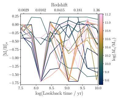
Figure 1: Mass-weighted mean stellar metallicity $[\rm M/H]_{*}$ in each age bin, determined by STARLIGHT, plotted as a function of lookback time for a random subsample of 20 galaxies. The line colour corresponds to the stellar mass of each galaxy. A flaw in the fitting process can be observed at a lookback time of $10^{8.15}\>\rm yr$ – namely that STARLIGHT is drawn to the lower bound of the stellar metallicity parameter space for this age bin. It is for this reason that we choose to exclude the SSP template with the lowest stellar metallicity value (i.e. $[\rm M/H]_{*}=-1.71$) at this specific age bin during the fitting process used to determine stellar metallicity histories in this work.

The steps described above allow the stellar mass history of each galaxy to be ascertained at each of the 15 template ages. The SFH of the galaxies can also be determined at each age bin by finding the difference in stellar mass between two ages, and then dividing this mass difference by the time span between bins. Finally, using a similar procedure, we can alternatively collapse the two-dimensional parameter space in the other dimension to form a one-dimensional function of mass-weighted stellar metallicity, which we use to obtain the mean value for the mass-weighted stellar metallicity history for each galaxy at the 15 template ages.

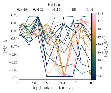
Figure 2: As Fig. 1 for the same random subsample of 20 galaxies, except now the problematic SSP template at $10^{8.15}\>\rm yr$ and $[\rm M/H]_{*}=-1.71$ is ignored during the STARLIGHT fitting process.

Since the galaxies which comprise the final sample used in this work are drawn from both the MaNGA Primary+ and Secondary samples (which obtain radial coverage out to $1.5\>\rm R_{e}$ and $2.5\>\rm R_{e}$ respectively; Bundy et al., 2015; Yan et al., 2016b), it is necessary to ensure that median stellar metallicities for galaxies in each of these samples can be compared with each other. Fortunately, the median value for the mass-weighted mean stellar metallicities for the Primary+ sample is $[\rm M/H]_{*}=-0.143$, while the corresponding value for the Secondary sample is $[\rm M/H]_{*}=-0.135$. Since there is not a substantial difference between these values, it is unlikely that the different radial coverage in the two samples has a significant influence on the results presented in this paper.

It is well known that some of the SSP templates are ill-constrained by the fitting process (Vazdekis et al., 2010; Vazdekis et al., 2016). In particular, low stellar metallicity templates with ages around ${\sim}10^{8}\>\rm yr$ are likely to fit systematic errors, such as residual flux calibration errors, rather than the data.

It is particularly difficult to produce reliable SSP templates for low metallicity populations. Creating these templates for populations that are dominated by intermediate age type B and A stars poses a challenge, since these stars are not only rare, but also contain very few metal lines in their spectra. Arguably, it is harder to create templates for these populations than those dominated by type O stars, since type B and A stars are vastly less luminous than their younger counterparts and hence their spectra are harder to observe. Like type O stars, the absence of metal lines makes the optical spectra of intermediate age populations poor stellar metallicity diagnostics. In fact, Vazdekis et al. (2010); Vazdekis et al. (2016) note that the templates of such stars flirt with being unreliable, as can be seen in Fig. 6 of Vazdekis et al. (2010) and Figs. 3 and 5 of Vazdekis et al. (2016). Both Fig. 6 of Vazdekis et al. (2010) and Fig. 3 of Vazdekis et al. (2016) show that the threshold age at which the quality of the SSP templates at $[\rm M/H]_{*}=-1.71$ drops into the “unsafe” range is almost exactly $10^{8.15}\>\rm yr$. Indeed, if we perform a fit to the spectra with all of the templates at our disposal (Fig. 1), we find that the lowest stellar metallicity template at a lookback time of $10^{8.15}\>\rm yr$ is hugely over-represented, leading to a systematic distortion in the stellar metallicity history of many galaxies. Such a drop is unphysical, and arises due to STARLIGHT latching on to the lowest stellar metallicity SSP template at this age, as this template is erroneously identified as the best fit for the galaxy. For an in-depth discussion about the reliability of the SSP templates used in this work, we refer the reader to Section 3.2 of Vazdekis et al. (2010), as well as Section 2 of Vazdekis et al. (2016).

The simplest course of action to try and address this issue is to exclude this lone problematic template at $10^{8.15}\>\rm yr$ prior to analysis. Throwing out this template does largely make the problem vanish, as can be seen in Fig. 2. While there may still be some residual issues at neighbouring ages, the stellar metallicities for both young ($\rm age<10^{8.15}\>\rm yr$) and old ($\rm age>10^{9.35}\>\rm yr$) populations do not appear to be at all affected by the removal of the SSP template at $10^{8.15}\>\rm yr$. Fortunately, since the young and old populations are not strongly coupled, they are robust against this potential systematic uncertainty – particularly when compared to the templates of intermediate age stars. Finally, it is encouraging to see that the mass-weighted mean stellar metallicities in both Fig. 1 and Fig. 2 converge to comparable, slightly sub-solar values at more recent lookback times. Despite our earlier concerns about whether the spectra of stars at such ages constitute reliable stellar metallicity diagnostics, this convergence means that we can now with confidence analyse mass-weighted mean stellar metallicities for populations dominated by stars in the range $10^{7.6}\>\rm yr\leq\rm age<10^{8.15}\>\rm yr$.

In short, whether or not this subset of troublesome SSPs is included in the fit makes essentially no difference to the results obtained in the age intervals considered in this work. Although some systematic residual effects are still apparent in Fig. 2, the worst of them have been mitigated. Comparing Figs. 1 and 2, we see that ages $<10^{8.15}\>\rm yr$ and $>10^{9.35}\>\rm yr$ are largely unaffected by these issues at intermediate ages. Accordingly, we can, with some confidence, compare the inferred mass-weighted mean stellar metallicities of galaxies at an age of $\rm 10^{9.95}\>\rm yr$ to those at the present day ($\rm age=10^{7.6}\>\rm yr$). This allows us to robustly study chemical evolution since cosmic noon. For a detailed description of some of the tests we performed to check that the fitting procedure undertaken in this work is sound, we refer the interested reader to Appendix A.

3.2 Gas Metallicities

The gas metallicities of the galaxies are determined in two separate ways in this work. The first – and most obvious – method by which gas metallicities are calculated is by measuring the strengths of various emission lines in the galaxies’ spectra. While this method is reasonably reliable, measuring the emission lines in these galaxies will naturally only allow the gas metallicities at the present day to be determined. In order to determine the gas metallicities of the galaxies at earlier times, we also employ the FMR of Mannucci et al. (2010). These two separate methods are expanded upon below.

3.2.1 Emission Lines

Although it is possible to directly measure the gas metallicity of a galaxy by measuring the strength of its ${\rm[\textsc{O~{}iii}]}\>\lambda 4363$ emission line, this line is very weak even in the best quality data and with the most appropriate chemical composition (e.g. Kewley & Ellison, 2008; Kewley et al., 2019). Furthermore, this so-called “direct method” may underestimate gas metallicities in both metal-rich galaxies (e.g. Stasińska, 2002, 2005; Bresolin et al., 2006) as well as metal-poor galaxies (e.g. Kobulnicky & Zaritsky, 1999).

For these reasons, we instead choose to estimate gas metallicities in this work via the use of strong-line methods. Many different theoretical calibrations have been developed to convert certain emission-line ratios, known to be sensitive to gas metallicities, into gas metallicity estimates. However, in order to obtain gas metallicities from the multitude of strong line calibrations available, these various diagnostics have to first be converted to a common calibration scale. Fortunately, Kewley & Ellison (2008) find that it is possible to convert a given gas metallicity diagnostic into any other calibration scheme via:

$$\log y=\sum_{n}c_{n}x^{n},$$ (1)

where $y$ is the original gas metallicity diagnostic to be converted in $12+\log(\rm O/H)$ units, the $c_{n}$ are $n$th-order polynomial coefficients to be optimised, and $x$ is the gas metallicity (specifically, the oxygen abundance) relative to solar metallicity (which we assume to be $12+\log(\rm O/H)_{\odot}=8.69$; Asplund et al., 2009). For the purposes of subsequent comparison with average stellar metallicities, we convert gas metallicities derived from emission line measurements from their $12+\log(\rm O/H)$ values to gas metallicity $\rm[M/H]_{g}$ via:

$$\rm[M/H]_{g}=\log\left(Z_{g}/Z_{\odot}\right)=12+\log(\rm O/H)-8.69,$$ (2)

(e.g. Sanders et al., 2021). Here, $Z_{\odot}$ is the Solar metallicity value ($Z_{\odot}=0.0142$; Asplund et al., 2009).

There are many available strong line calibrations: see, for instance, Kewley & Ellison (2008) for a comprehensive study comparing various different strong line calibrations, as well as to Scudder et al. (2021) for a similar, more recent study exclusive to MaNGA galaxies. However, according to both Kewley & Ellison (2008) and Kewley et al. (2019), the $\rm N2O2$ ratio – defined as $\rm[\textsc{N~{}ii}]\>\lambda 6584/[\textsc{O~{}ii}]\>\lambda\lambda 3727,\>3729$ – is by far the most reliable optical gas metallicity diagnostic. Not only is it robust (Paalvast & Brinchmann, 2017), but it also does not depend on the ionisation parameter (e.g. Kewley & Dopita, 2002; Blanc et al., 2015). The $\rm N2O2$ ratio is highly sensitive to gas metallicity for two reasons: firstly, because nitrogen may be formed by both primary and secondary nucleosynthesis processes (e.g. Considère et al., 2000; Kewley et al., 2019); secondly, because the $[\textsc{O~{}ii}]\>\lambda\lambda 3727,\>3729$ line is very sensitive to electron temperature (e.g. Hägele et al., 2008; Kewley et al., 2019). The $\rm N2O2$ ratio depends on ISM pressure only at very high gas metallicities $\left[12+\log(\rm O/H)>9.23\right]$ and at the highest ISM pressures (Kewley et al., 2019). Finally, the $\rm N2O2$ ratio is also the least sensitive optical diagnostic to the presence of an active galactic nucleus (Kewley et al., 2006) or diffuse ionised gas (Zhang et al., 2017).

While gas metallicities are derived from oxygen abundances (cf. Equation 2), stellar metallicities, by contrast, trace the iron abundance of stars (e.g. Tinsley, 1980; Maiolino & Mannucci, 2019). Therefore, in order to treat the metallicities of the stellar populations and the gas from which these formed on equal footing, we must transform our elemental abundance base. Fortunately, Fraser-McKelvie et al. (2022) have demonstrated that it is possible to convert gas metallicities into an iron base using the scaling relations of Nicholls et al. (2017) as follows:

$${\rm[M/H]_{g,\>iron}} =0.9941\times(12+\log(\rm O/H))-8.9011,$$ (3)

$$\ \ \ (\rm if\ 12+\log(\rm O/H)-8.69>-0.5),$$

$$=0.6753\times(12+\log(\rm O/H))-8.6875,$$

$$\ \ \ (\rm if\ 12+\log(\rm O/H)-8.69<-0.5),$$

(A. Fraser-McKelvie, private communication). Throughout the rest of this paper, any $\rm[M/H]_{g}$ values quoted will be understood to be scaled to an iron base, unless otherwise stated.

In this work, we use the best-fit coefficients calculated by Kewley & Dopita (2002) in Equation (1) to estimate the present-day gas metallicities of the MaNGA galaxies from measurements of the $\rm N2O2$ line ratio. Since – as Kewley & Ellison (2008) caution – the absolute gas metallicity determined from any particular strong-line method should not be trusted, the final step is to calibrate the gas metallicities calculated in this work to the stellar mass–gas metallicity relation ($\rm MZ_{g}R$) of Tremonti et al. (2004). This is done by forcing the best fit line to our data to have the same value for the gas metallicity predicted by the $\rm MZ_{g}R$ of Tremonti et al. (2004) at a stellar mass of $10^{10}\ \rm M_{\odot}$. Doing so decreases the calculated gas metallicities by $0.3\>\rm dex$. Note that the $\rm MZ_{g}R$ is distinct from the stellar mass–stellar metallicity relation, which we denote $\rm MZ_{*}R$ throughout this paper for the sake of clarity.

3.2.2 The Fundamental Metallicity Relation

Since the aim of this paper is to compare the chemical evolution of the stars and the gas within spiral galaxies, we require an alternative method for determining the gas metallicities at epochs earlier than the present day. To this end, we turn to the FMR obtained by Mannucci et al. (2010), who demonstrate that the gas metallicity of a galaxy may be estimated if both its stellar mass, $M_{*}$, and its SFR are known:

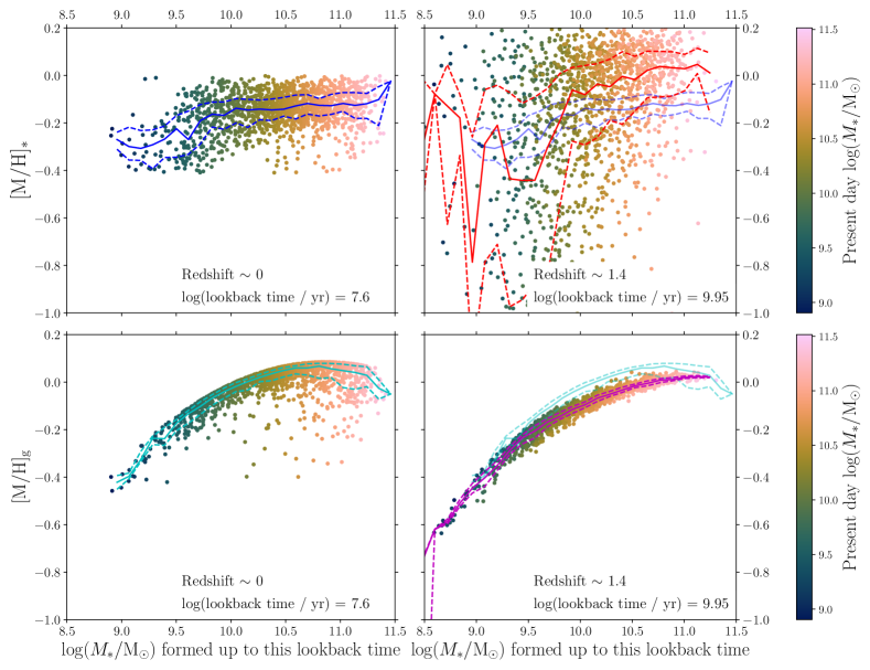
Figure 3: Mass–metallicity relations for the sample of MaNGA galaxies. Individual galaxies are coloured by their present-day stellar masses. The horizontal axis shows the mass in stars that has formed up to a certain lookback time. The plots on the top row show mass-weighted mean stellar metallicity as a function of stellar mass, while the plots on the bottom row show gas metallicity as a function of stellar mass. The data in the left-hand column are from the youngest age bin at a lookback time of $10^{7.6}\>\rm yr$, while the right-hand column shows data from the oldest age bin at a lookback time of $10^{9.95}\>\rm yr$. The running medians (solid lines) and running inter-quartile ranges (dashed lines) to the mass-weighted mean stellar metallicity data at high and low redshift are overplotted in red and blue, respectively. Similarly, the equivalent lines for the gas metallicities at high and low redshift are overplotted in magenta and cyan, respectively.

$$12+\log(\rm O/H)= \ 8.90+0.37m-0.14s-0.19m^{2}$$ (4)

$$+0.12ms-0.054s^{2}.$$

Here, $m=\log\left(M_{*}\right)-10$, with $M_{*}$ measured in units of $\rm M_{\odot}$; and $s=\log\left(\rm SFR\right)$, with SFR measured in units of $\rm M_{\odot}\ yr^{-1}$. Mannucci et al. (2010) find that the FMR does not evolve until a redshift of $z\sim 2.5$, while Sanders et al. (2021) conclude that there is no evolution in the FMR until $z\sim 3.3$. Therefore, we can use Equation (4) to comfortably estimate the gas metallicities of galaxies as far back as the largest lookback time we consider in this work, $10^{9.95}\>\rm yr$ ($z\sim 1.4$). Again, we convert all gas metallicities determined by using the FMR into $\rm[M/H]_{g}$ values, before calibrating the present-day values against the $\rm MZ_{g}R$ calculated by Tremonti et al. (2004), as described in Section 3.2.1. This calibration results in a decrease in $\rm[M/H]_{g}$ of $0.31\>\rm dex$ at the present day.

Reassuringly, as we shall see from the analysis in Section 4.2, gas metallicities inferred from the FMR at recent epochs agree very well with those obtained directly from the gas itself via measurements of the N2O2 line ratio.

4 Results and Discussion

We first plot the mass–metallicity relations for both the stellar populations and the gaseous ISM at low and high redshifts. This also allows us to determine how both the $\rm MZ_{*}R$ and the $\rm MZ_{g}R$ of the sample galaxies evolve over cosmic time. We then explore the ramifications of these results further by investigating how stellar mass influences the evolution of the average stellar and gas metallicities of these galaxies.

4.1 Evolution of the Mass–Metallicity Relations

Figure 3 shows mass–metallicity relations for the sample of 1619 MaNGA galaxies. Plots on the top row show the mass-weighted mean stellar metallicities for each of the sample galaxies, and plots on the bottom row show gas metallicity data. The plots in the left-hand column show the $\rm MZ_{*}R$ and the $\rm MZ_{g}R$ at the closest lookback time to the present day, $10^{7.6}\>\rm yr$ ($z\sim 0$), while those in the right-hand column show how both the mass–metallicity relations were at a lookback time of $10^{9.95}\>\rm yr$ ($z\sim 1.4$).

There are two kinds of uncertainties that we have to consider in Fig. 3. The first kind are the random errors from the scatter in the data used to construct the plots of Fig. 3. The second kind of uncertainties are systematic errors in the $\rm MZ_{*}R$. Although these errors are fundamentally unquantifiable, fortunately they will at least all be internally consistent at all redshifts, since we have determined the $\rm MZ_{*}R$ in exactly the same way both at low and high redshift.

The gas metallicities exhibit a much tighter relationship with stellar mass than do the mass-weighted mean stellar metallicities. This is because they are estimated (via the FMR – see Equation 4) using just two input parameters: the stellar mass and the SFR at a particular age. This means that the tight relationship in the $\rm MZ_{g}R$ is actually a consequence of the tight relationship between stellar mass and SFR. In order to test how reliably the FMR reproduces the $\rm MZ_{g}R$, we investigated at both low and high redshift the relationship between stellar mass and SFR. Reassuringly, the evolution in this parameter space from high to low redshift was found to be in good agreement with that reported by Speagle et al. (2014). Additionally, to further verify that the FMR robustly reproduces the $\rm MZ_{g}R$ at low redshift, we also independently derived the $\rm MZ_{g}R$ at $z\sim 0$ using the N2O2 calibrator of Kewley & Dopita (2002) – see Section 3.2.1 – and found that these two different methods yielded consistent relationships between stellar mass and gas metallicity

Figure 3 shows that the evolution of the $\rm MZ_{g}R$ between $z\sim 1.4$ and $z\sim 0$ is marginal; nevertheless, the $\rm MZ_{g}R$ is seen to increase to higher average gas metallicity values between a redshift of $z\sim 1.4$ and the present day. This result is in line with many authors who have previously studied the redshift evolution of the $\rm MZ_{g}R$ – for instance Maiolino et al. (2008); Moustakas et al. (2011); Zahid et al. (2013b, 2014); Lian et al. (2018a); Lian et al. (2018b); and Yates et al. (2021). In particular, the $\rm MZ_{g}R$ at $z\sim 0$ shown in Fig. 3 is in very good agreement with the results reported by both Fontanot et al. (2021) and Curti et al. (2020), the latter of which find a peak O/H value of ${\sim}0.1$ dex above Solar, just as we report here. While our $\rm MZ_{g}R$ at $z\sim 1.4$ is systematically lower than that reported by Fontanot et al. (2021), it is still within their range of uncertainty (see also the large spread of observational results from different authors such as Zahid et al., 2014, Yabe et al., 2015, and Curti et al., 2020).

A similar evolution in the $\rm MZ_{*}R$ has been found from semi-analytic modelling performed by Yates et al. (2021), as well as at a high redshift range of $1.6\leq z\leq 3.0$ by Kashino et al. (2022). Observational results at low redshifts from authors such as Camps-Fariña et al. (2021, 2022) and Fontanot et al. (2021) also show that the $\rm MZ_{*}R$ does indeed evolve from high to low redshift, with high-mass galaxies found to evolve faster than low-mass ones. It is important to note, however, that Camps-Fariña et al. (2021, 2022) also find that the chemical evolution history of a galaxy may be strongly influenced by other fundamental properties, such as their stellar masses and morphologies. In addition, Beverage et al. (2021) find that the $\rm MZ_{*}R$ may not evolve with redshift at all, depending on the elemental abundance concerned.

It can be seen from Fig. 3 that there has been little evolution in the median $\rm MZ_{*}R$ with redshift since a lookback time of ${\sim}10^{9.95}\>\rm yr$. While a similar lack of evolution in the $\rm MZ_{*}R$ over this time period is reported by Panter et al. (2008) and Vale Asari et al. (2009), other authors, such as Camps-Fariña et al. (2021, 2022) show that $[\rm M/H]_{*}$ has decreased since this lookback time. However, the overall spread of the $\rm MZ_{*}R$ clearly does evolve with redshift. Fundamentally, there is a very large spread in the observed mass-weighted mean stellar metallicities of galaxies, particularly at higher redshifts. This can be seen in this work in the top-right plot of Fig. 3, as well as in work by previous authors such as Gallazzi et al. (2005); Panter et al. (2008); and Beverage et al. (2021). The spread of the data in this top-right plot is very similar to the $\rm MZ_{*}R$ found by Panter et al. (2008). By contrast, the spread of the data in the low-redshift $\rm MZ_{*}R$ is much tighter, a result also reported at low redshift by Fontanot et al. (2021) – though note the spread of the data in our high-redshift $\rm MZ_{*}R$ is larger than that reported at high redshift by these same authors. The range of our average stellar metallicities in the top-left plot of Fig. 3 is between $-0.4$ and $0.0$ dex, and the median $\rm MZ_{*}R$ reaches roughly solar abundance at the very high-mass end, in agreement with previous authors including Zahid et al. (2017) and Fontanot et al. (2021).

In essence, as we move closer to the present day, the mass-weighted mean stellar metallicities exhibit a much tighter relation with stellar mass, and are comparable to the observed gas metallicities; the data here are actually in much better agreement with the $\rm MZ_{g}R$ of Tremonti et al. (2004). Such a finding is in accord with previous work by authors such as González Delgado et al. (2014), Sánchez et al. (2018), and Lacerda et al. (2020), each of whom find good agreement between the $\rm MZ_{g}R$ and the $\rm MZ_{*}R$ at young stellar ages. This makes sense when we recall that this is the gas from which these same stars are forming. That the mass-weighted mean stellar metallicities converge in this manner over cosmic time is not a consequence of our sample selection; in reality it is a consequence of the rich and varied chemical evolution histories of the individual galaxies over several generations of star formation. As Fraser-McKelvie et al. (2022) explain, the difference between stellar and gas metallicities at early cosmic times is dependent on the SFH of the galaxy. Galaxies that reach their peak SFR at later times take longer to accumulate metals, and so $[\rm M/H]_{*}\ll[\rm M/H]_{g}$ (Fraser-McKelvie et al., 2022).

The analysis presented in this work ultimately represents a step forward over complementary methodology by which gas metallicities are also observationally determined – i.e. obtaining snapshots of the metallicity of the gas in various galaxies at increasing redshifts. While the quality of data obtained via these snapshots decreases with increasing redshift, this alternative method of galactic archaeology, by contrast, acquires high-quality measurements of the gas metallicity back to distant lookback times, as seen in Fig. 3. Such analysis is similar to that which has already been carried out for the stellar metallicity histories of galaxies by authors such as Peterken et al. (2019, 2020), Camps-Fariña et al. (2021, 2022), and Fraser-McKelvie et al. (2022). Furthermore, since we are tracking the evolution of the gas (as well as the stellar populations) from observations made in very low-redshift galaxies, we are also able to check the validity of our archaeological approach against present-day emission-line data in these same galaxies. This concept is explored further in Section 4.2.

4.2 How does Stellar Mass Affect Metallicity Evolution?

In order to investigate how stellar mass influences metallicity evolution, we now turn to Fig. 4, which shows how both mass-weighted mean stellar metallicity, $[\rm M/H]_{*}$, and gas metallicity, $[\rm M/H]_{g}$, have evolved with cosmic time since cosmic noon. We have divided the galaxies into five logarithmically-spaced stellar mass bins, and calculated the median of the gas and mass-weighted mean stellar metallicity for each mass bin. The star-shaped datapoints are generated using mass-weighted mean stellar metallicity data from STARLIGHT, and gas metallicity data from the FMR of Mannucci et al. (2010); these evolve from a lookback time of $10^{9.95}\>\rm yr$ through to $10^{7.6}\>\rm yr$. The open circles show – as a comparison – the same stellar metallicities at a lookback time of $10^{7.6}\>\rm yr$, but plotted instead against the present-day gas metallicities that have been directly determined from measurements of the N2O2 ratio. These emission line data are included only as a consistency check to ensure that the data derived from the FMR (at the present day) are sensible. The two complementary methods for determining gas metallicities at the present epoch yield consistent values for galaxies in all mass bins. To summarise, Fig. 4 represents the ultimate result of the co-evolution of gas and stellar metallicity that we originally set out to measure. As mentioned in Section 3.2.2, the good agreement between the present-day gas metallicity derived from the FMR and that measured directly from emission lines gives some confidence in the validity of this approach.

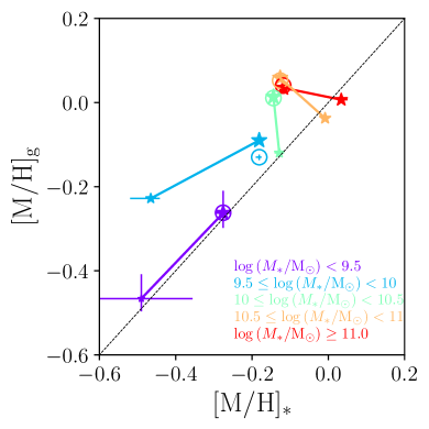
Figure 4: Evolution of stellar and gas metallicities with cosmic time. The median metallicities for the sample galaxies are determined for five different stellar mass bins. Three datapoints are plotted for each mass bin. Star-shaped datapoints denote mass-weighted mean stellar metallicity data derived from STARLIGHT and gas metallicity data from the FMR of Mannucci et al. (2010). The size of the star is proportional to the fraction of mass that had formed at that redshift. The larger stars therefore correspond to a lookback time of $10^{7.6}\>\rm yr$ ($z\sim 0$), and the smaller stars to a lookback time of $10^{9.95}\>\rm yr$ ($z\sim 1.4$). The open circles plot the stellar metallicities of the mass bins at a lookback time of $10^{7.6}\>\rm yr$ against the present-day gas metallicities derived from measurements of the N2O2 ratio (Kewley & Dopita, 2002) to ensure the gas metallicities predicted by the FMR are plausible. The errorbars show the $1\sigma$ uncertainty on the median of each datapoint. The black diagonal line is a 1-to-1 relation, and does not represent a fit to the data.

In interpreting these results, let us first consider those spiral galaxies with stellar masses less than $10^{10}\ \rm M_{\odot}$. Generically, these galaxies are seen to increase both their stellar and gas metallicities since cosmic noon. The increases in the median gas metallicities are consistent with those measured by Panter et al. (2008) and Maiolino et al. (2008), and similar increases in stellar metallicities over this time period are also seen by Camps-Fariña et al. (2021, 2022). While certain authors, such as Sánchez Almeida (2017), Sánchez-Menguiano et al. (2019), and Belfiore et al. (2019b), have reported that gas accretion may in fact play an important role in galactic evolution, even in low-mass systems, the findings presented in this paper fit in well with the results from recent work (Greener et al., 2021; see also Mejía-Narváez et al., 2020 and the semi-analytic spectral fitting performed by Zhou et al., 2022), in which we conclude that such relatively low-mass spiral galaxies tend to evolve as closed boxes (i.e. very little or no gas flows into or out of the galaxy over the course of its life – see Talbot & Arnett, 1971 and Tinsley, 1974).

Within the context of these results, the behaviour of the low-mass spiral galaxies in Fig. 4 is to be anticipated. Since these low-mass galaxies evolve as closed boxes but are still forming stars at the present epoch, they must be forming stars over much longer timescales than their high-mass counterparts. Previous authors, such as Vale Asari et al. (2007), have attributed the languid star formation within such galaxies to their proportionally lower gas metallicities (see Fig. 4). However, it is more likely that the low stellar masses of such galaxies are actually the driving force behind their lengthy star formation timescales (Greener et al., 2021; Peterken et al., 2021; see also Camps-Fariña et al., 2021, 2022 and Fraser-McKelvie et al., 2022), since stellar mass is the dominant factor influencing the gas metal content of galaxies (e.g. Tremonti et al., 2004). This leisurely pace allows these low-mass galaxies to thoroughly mix their gas between stellar generations, and thus they steadily increase both the metallicity of their stars – and the ISM which these stars pollute – over cosmic time, exactly as we see in Fig. 4.

Figure 4 shows that high-mass galaxies have also increased their median gas metallicities since $z\sim 1.4$ (albeit less dramatically than their low-mass counterparts; again, this is consistent with the direct measurements made by Panter et al., 2008, Maiolino et al., 2008, and Camps-Fariña et al., 2021, 2022). In Greener et al. (2021), we showed that a spiral galaxy with a stellar mass greater than $10^{10}\ \rm M_{\odot}$ is far more likely to behave instead as an accreting box rather than a closed box. The accreting box model is similar to that of a closed box, but additionally allows for a steady stream of pristine gas to flow into the galaxy over time (Larson, 1972, 1976; Tinsley, 1974, 1980). Moreover, if galaxies do not accrete pristine gas, their star formation quenches rapidly; this effect is also far more pronounced for higher mass galaxies in the epoch since cosmic noon (E. Taylor et al. 2022, submitted).

This infall of metal-poor gas allows these galaxies to produce a significant quantity of high-mass stars, which, upon their deaths, pollute the ISM with newly-forged metals. Subsequent generations of stars will be formed from this enriched material, which ultimately means that over cosmic time, the gas metallicity of high-mass galaxies gradually increases.

We might expect that the stellar populations in high-mass galaxies should be similarly enriched over cosmic time; however, Fig. 4 demonstrates that the median stellar metallicity of such galaxies decreases at later times. This is a surprising result, and is in disagreement with other authors such as Panter et al. (2008) – who find essentially no change in the average stellar metallicity over this redshift interval – and Camps-Fariña et al. (2021, 2022) – while these authors do report a decrease in the average stellar metallicity since ${\sim}10^{9.75}\>\rm yr$, this decrease is less pronounced than that which we report here. Why should this be? High-mass galaxies must accrete largely unmixed pristine gas over their lifetimes in order to satiate the demand required to maintain star formation at later times. Furthermore, these galaxies have been found to form the majority of their stars at earlier times (e.g. Beverage et al., 2021; Peterken et al., 2021; Zhou et al., 2021; Fraser-McKelvie et al., 2022).

The decrease in the median stellar metallicities of these galaxies over cosmic time could, therefore, be a direct consequence of the pristine gas that they accrete. If this gas is not well mixed into the galaxy, it is probable that metal-poor stars will continuously form, even at very late times. These stars will still pollute the ISM with metals upon their deaths, raising the average metallicity of the gas in these galaxies over time; however, even at late times the average stellar metallicity may be suppressed if such metal-poor stars always form from the supply of pristine gas. Further work will be required to investigate whether the average stellar metallicities observed in high-mass galaxies in this work at the redshift of $z\sim 1.4$ around cosmic noon represents a local maximum, or whether the median stellar metallicities of such galaxies increases yet further at even higher redshifts.

5 Conclusions

We investigate the chemical evolution histories of both the stellar populations and the gas for a well-defined sample of 1619 spiral galaxies observed by MaNGA. Mass-weighted mean stellar metallicities are determined at low ($z\sim 0$) and high ($z\sim 1.4$) redshifts via the use of the full-spectrum stellar population synthesis code STARLIGHT (Cid Fernandes et al., 2005); gas metallicities are estimated at the same epochs using the FMR of Mannucci et al. (2010). We also calculate the present-day gas metallicities of the same galaxies by using the strong-line N2O2 calibration proposed by Kewley & Dopita (2002).

The evolution of both the $\rm MZ_{*}R$ and the $\rm MZ_{g}R$ are examined and discussed, in addition to the mass-dependence of the average stellar and gas metallicities of the galaxies. The results of these investigations are summarised below.

1. The $\rm MZ_{g}R$ is generically found to evolve in such a way that at a given mass, the gas within the galaxies becomes increasingly metal-rich with cosmic time. This result is in agreement with the findings of Maiolino et al. (2008), Moustakas et al. (2011), Zahid et al. (2013b, 2014), Lian et al. (2018a); Lian et al. (2018b), and Yates et al. (2021). Unlike the methods by which these authors determine the evolution of the $\rm MZ_{g}R$, however, the method used in this work of tracking the evolution of the gas within low-redshift galaxies back to more distant lookback times via galactic archaeology allows for high-quality measurements of the gas metallicity even at high redshifts.

2. The median $\rm MZ_{*}R$ exhibits a general decline in stellar metallicity from $z\sim 1.4$ to $z\sim 0$, for the bulk of the explored sample, with the possible exception for the mass range $M_{*}<10^{10}\>\rm M_{\odot}$, in which little to no evolution is seen. The shape of the $\rm MZ_{*}R$ also changes: it is steeper at $z\sim 1.4$ and shallower at $z\sim 0$. The spread of the mass-weighted mean stellar metallicity data – comparable to that found by Gallazzi et al. (2005), Panter et al. (2008), and Beverage et al. (2021) – also evolves with cosmic time: the $\rm MZ_{*}R$ exhibits a much tighter relation at later times. In fact, at $z\sim 0$, the observed $\rm MZ_{*}R$ is more comparable to the $\rm MZ_{g}R$ of Tremonti et al. (2004) than, for instance, the $\rm MZ_{*}R$ of Panter et al. (2008), since these stars are forming from the same gas whose emission lines authors such as Tremonti et al. (2004) observe.

3. The results in this paper align well with those found in recent work (Greener et al., 2021), in which we conclude that low-mass spirals evolve as closed boxes, whereas high-mass spirals accrete a stream of relatively pristine gas over the course of their lives. We find in this work that low-mass galaxies steadily increase their stellar and gas metallicities over cosmic time since they form stars relatively slowly and are parsimonious with their gas reservoirs. High-mass galaxies, by contrast, have lower average stellar metallicities at later times. If the pristine gas is not particularly well-mixed into the galaxy upon accretion, large numbers of metal-poor stars will readily form in that galaxy even at very late times. This could result in the average stellar metallicities in high-mass spiral galaxies being suppressed at the present epoch.

Data Availability

This publication uses MPL-11 MaNGA science data products. The full sample of data used in this paper has recently been made completely accessible as part of the public release of SDSS DR17 (Abdurro’uf et al., 2022).

Appendix A Additional Tests of the Spectral Fitting Outputs

In order to verify that the mass-weighted mean stellar metallicities and SFRs obtained from the STARLIGHT fitting procedure are reliable – even after removing the problematic SSP template at $\log(\rm age/yr)=8.15$ and $[\rm M/H]_{*}=-1.71$ prior to analysis (as described in detail in Section 3.1) – we have undertaken several tests which we describe in detail below.

A1 Comparing Best-Fit Spectra

STARLIGHT uses Monte Carlo techniques to derive best-fit spectra for the input spectra of each of the spaxels in the sample galaxies, with no assumptions made on the shape of the derived star formation histories (Cid Fernandes et al., 2005). Each best-fit spectrum is created from a linear combination of a set of input SSP template spectra and an applied dust attenuation. We wish to test whether the resulting best-fit spectrum produced for a given galaxy is affected by the removal of a single SSP template at $\log(\rm age/yr)=8.15$ and $[\rm M/H]_{*}=-1.71$.

The upper plot of Fig. A1 compares – for each of three randomly selected sample galaxies of varying signal-to-noise ratio (S/N) levels – the raw MaNGA spectrum (black line), the best-fit spectrum produced by STARLIGHT if all the SSP templates (described in Section 3.1) are included in the fitting procedure (light coloured line), and the equivalent best-fit spectrum if the problematic SSP template at $\log(\rm age/yr)=8.15$ and $[\rm M/H]_{*}=-1.71$ is excluded prior to the fitting procedure (dark coloured line). For each of the three galaxies, the fluxes of the best-fit spectra have been arbitrarily offset to either side of the raw MaNGA spectrum so that each of the spectra are clearly visible; otherwise, both spectra would be plotted almost exactly on top of each other for a given galaxy.

The lower plot of Fig. A1 shows – for each of the three galaxies – the flux residuals between the raw MaNGA spectrum and the two best-fit spectra described above. Again, each pair of flux residuals – and their respective black baselines – have been arbitrarily vertically offset from each other, so that both can be clearly seen.

The upper plot of Fig. A1 indicates that removing the troublesome SSP prior to the STARLIGHT fitting procedure makes essentially no discernible difference to the best-fit spectra of any of the three galaxies: for each of the three galaxies, the two best-fit spectra shown are almost identical to each other. Furthermore, the flux residuals for these galaxies tell a similar story: the residuals between the raw MaNGA spectrum and the two best-fit spectra for each galaxy are so similar as to be virtually indistinguishable.

In short, this test demonstrates that the best-fit spectrum produced by STARLIGHT for a given MaNGA galaxy is very unlikely to be affected by the removal of the lone SSP template at $\log(\rm age/yr)=8.15$ prior to analysis.

A2 Comparison of Stellar Metallicities

As explained in Section 3.1, the result of the STARLIGHT fitting process is a set of weights for the mass contributions of SSPs with different ages and chemical compositions to the light seen in the spectrum of each spaxel across the face of a galaxy. In this work, we use these weights to derive mass-weighted mean stellar metallicities and SFHs for the sample galaxies.

In order to test whether the mass-weighted mean stellar metallicities obtained in this work are reliable, we compared our values to those from two different Value Added Catalogues (VACs), both of which provide spatially-resolved stellar population properties for the full set of MaNGA galaxies included in the seventeenth (and final) SDSS-IV data release (DR17; Abdurro’uf et al., 2022). One VAC uses the full spectral fitting code Fitting IteRativEly For Likelihood analYsis (FIREFLY; Wilkinson et al., 2017), and its data products are described in full by Goddard et al. (2017) and Neumann et al. (2022); the other VAC uses the software Pipe3D (Sánchez et al., 2016a, b), and the data products are detailed fully in Lacerda et al. (2022) and Sánchez et al. (2022).

Figures A2 and A3 compare the median mass-weighted stellar metallicities calculated in this work with stellar metallicity values provided by the FIREFLY (Goddard et al., 2017; Neumann et al., 2022) and Pipe3D (Lacerda et al., 2022; Sánchez et al., 2022) VACs. The left-hand and central plots show stellar metallicity data for sample galaxies from the FIREFLY VAC within a shell located at 1 $\rm R_{e}$ and within a diameter of $3^{\prime\prime}$, respectively; the right-hand plots, meanwhile, show stellar metallicity data from the Pipe3D VAC. Confidence contours of $1\sigma$, $2\sigma$, and $3\sigma$ are drawn for each of these comparative plots. The histograms plot the density distribution of the difference between the median mass-weighted stellar metallicities calculated in this work, and those from the various VAC data (denoted $\Delta_{[\rm M/H]_{*}}$). The mean value of this difference, $\langle\Delta\rangle$, is also quoted in each instance.

Both of these Figures display very similar data. Figure A2 shows a comparison of the stellar metallicity data calculated in this work at a lookback time of $10^{7.6}\>\rm yr$ with the various VAC data; whereas Fig. A3 instead plots a similar comparison of the stellar metallicity data calculated in this work at a lookback time of $10^{9.95}\>\rm yr$.

At small ($10^{7.6}\>\rm yr$; Fig. A2) lookback times, corresponding to young stellar components, the stellar metallicity data obtained in this analysis are less well correlated with the various VAC data than at high ($10^{9.95}\>\rm yr$; Fig. A3) lookback times, corresponding to old stars. Indeed, at high lookback times, the correlation between our data and those of the various VACs improves significantly, lying close to the 1-to-1 relation and becoming a fairly tight relationship. This is not too surprising: at progressively younger stellar ages, the metallicities of a stellar population will become increasingly akin to the metallicity of the gas from which it is forming (cf. Section 4.1), and the difficulties of deriving stellar metallicities for very young stars are equally difficult and uncertain for all the three methods compared here. Therefore, we would expect to see a better correlation between the stellar metallicity data in this work and those from the VACs at higher lookback times – which is apparent in the different shapes of the confidence contours in Fig. A2 and in Fig. A3.

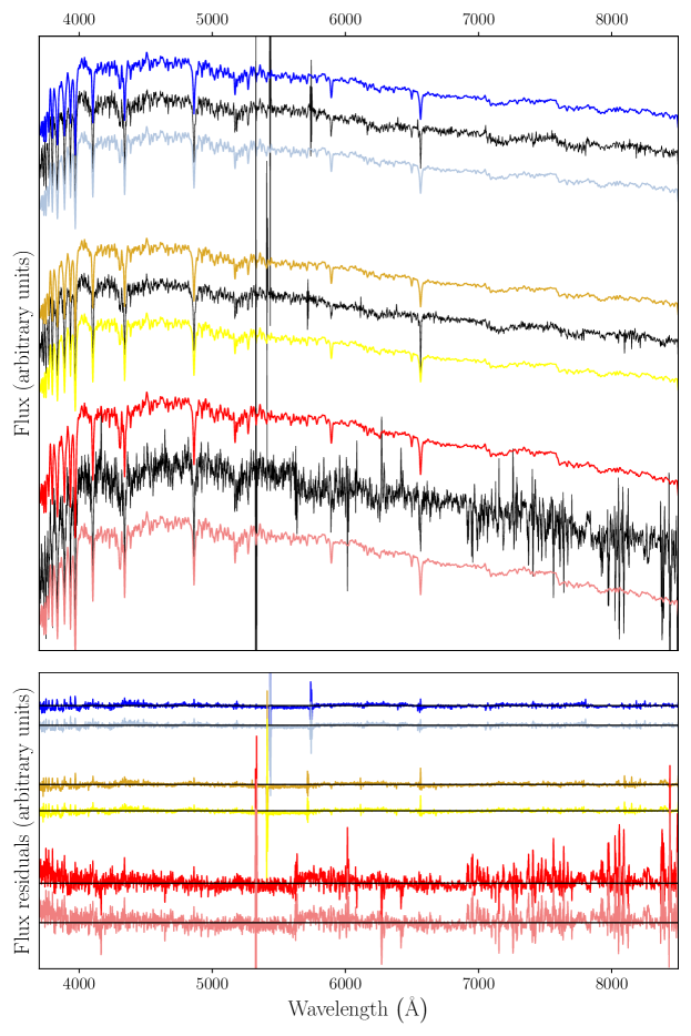
Figure A1: Example spectra (upper plot) and residuals (lower plot) for three randomly selected sample galaxies with varying S/N levels. Blue spectra are those of galaxy 9499-6102 ($\rm S/N=93.4$); yellow spectra are those of galaxy 9024-6102 ($\rm S/N=46.2$); red spectra are those of galaxy 8619-12703 ($\rm S/N=26.2$). Black lines show the raw MaNGA spectra for each of these three galaxies. Light coloured lines (plotted below the corresponding black spectra) show the best-fit spectra (upper plot), and residuals between these spectra and the raw MaNGA spectra (lower plot), produced by STARLIGHT if all the SSP templates are included in the fitting procedure. Dark coloured lines (plotted above the corresponding black spectra) show the best-fit spectra and residuals if the problematic SSP template at $\log(\rm age/yr)=8.15$ and $[\rm M/H]_{*}=-1.71$ is excluded from the fitting procedure (cf. Section 3.1). Note that the vertical axis, showing the flux of the stellar spectra, is arbitrary, since spectra are offset from each other by arbitrary amounts for the sake of clarity. Almost no differences can be seen between either any of the three pairs of best-fit spectra or any of their residuals.

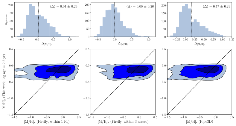
Figure A2: The vertical axis of these plots shows median mass-weighted stellar metallicities calculated for the sample galaxies in this work at a lookback time of $10^{7.6}\>\rm yr$. These data are compared with stellar metallicities calculated for the same galaxies provided by the FIREFLY VAC of DR17 galaxies (Goddard et al., 2017; Neumann et al., 2022) calculated within a shell located at 1 $\rm R_{e}$ (left-hand plots); with stellar metallicities provided by the same FIREFLY VAC calculated within a diameter of $3^{\prime\prime}$ (central plots); and finally with stellar metallicities provided by the Pipe3D VAC of DR17 galaxies (Lacerda et al., 2022; Sánchez et al., 2022, right-hand plots). The lower plots show confidence contours of $1\sigma$, $2\sigma$, and $3\sigma$ for the data, with the 1-to-1 relation shown by the dashed black diagonal line. The corresponding upper plots show histograms plotting the density distribution of the difference between our median mass-weighted stellar metallicity data and those from the VACs cited above, $\Delta_{[\rm M/H]_{*}}$. The mean value of this difference, $\langle\Delta\rangle$, and its standard deviation, are also shown in these upper plots.

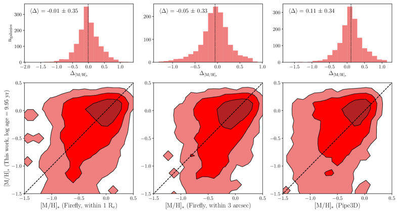
Figure A3: As Fig. A2, except that the median mass-weighted stellar metallicities plotted on the vertical axis are instead calculated for the sample galaxies in this work at a lookback time of $10^{9.95}\>\rm yr$. The data plotted on the horizontal axes are the same as in Fig. A2.

Reassuringly, however, the mean value of $\Delta_{[\rm M/H]_{*}}$ is consistent with a mean of zero (within the range of the quoted uncertainty) for each of the six comparisons made across both sets of Figures at the different lookback times. This statistic implies that the mass-weighted mean stellar metallicities calculated during the STARLIGHT fitting process are in agreement with stellar metallicities provided by both the FIREFLY and Pipe3D VACs. The dispersion in the mean $\Delta_{[\rm M/H]_{*}}$ ranges from 0.26 to 0.35, which corresponds to ${\sim}30\%$ of the dynamical range covered by the sampled parameter. These mean $\Delta_{[\rm M/H]_{*}}$ statistics show higher dispersions than that found when comparing FIREFLY and Pipe3D data against each other; Sánchez et al. (2022) report a mean value of $\Delta_{[\rm M/H]_{*}}=0.21\pm 0.16$. The standard deviations reported are up to twice as high as those expected from simulations when using STARLIGHT (see both Cid Fernandes et al., 2014 and González Delgado et al., 2014).

A3 Comparison of Star Formation Rates

In this work, we use SFHs derived by the STARLIGHT fitting procedure to trivially determine the SFRs of the sample galaxies at different lookback times. It is therefore crucial to ensure that the SFRs used throughout this work are reasonably accurate. In order to test the reliability of these SFRs that we employ, we can produce a similar plot to those discussed in Section A2 and assess the data accordingly.

We can derive an alternative and independent value for the present-day SFR by measuring the intrinsic $\rm H\alpha$ flux – provided by the MaNGA DAP – for each of the sample galaxies. This procedure is described fully by Greener et al. (2020), but in essence, we first correct the raw $\rm H\alpha$ flux for dust attenuation using measurements of the Balmer decrement (defined as the flux ratio of $\rm H\alpha$ to $\rm H\beta$) at each star-forming spaxel within a given galaxy and by employing the reddening curve of Calzetti et al. (2000). We then use the total galactic dust-corrected $\rm H\alpha$ flux in conjunction with luminosity distances provided by the NASA Sloan Atlas catalogue (Blanton et al., 2011) to obtain the $\rm H\alpha$ luminosity in Watts, $L_{{\rm H\alpha}}\>{\rm\left[W\right]}$, for each of the sample galaxies. The $\rm H\alpha$ derived SFR, $\rm SFR_{H\alpha}$, for each galaxy is then calculated using the Kennicutt (1998) relation:

$${\rm SFR_{H\alpha}}\>\left[{\rm M_{\odot}\ yr^{-1}}\right]=\frac{L_{{\rm H\alpha}}\>{\rm\left[W\right]}}{2.16\times 10^{34}\>\rm M_{\odot}\ yr^{-1}}.$$ (5)

Since we obtain an estimate for the $\rm H\alpha$ derived SFR via the measurement of nebular emission lines, it makes sense to compare $\rm SFR_{H\alpha}$ with the SFR calculated by STARLIGHT only at the youngest stellar age – a lookback time of $10^{7.6}\>\rm yr$. This is not only because such emission lines are produced at the present day, but also because only the young type O and B stars will have temperatures sufficient to ionise the neutral hydrogen gas which surrounds them into H ii regions, thus producing the nebular emission lines we require to measure the $\rm H\alpha$ derived SFRs of their host galaxies.

Figure A4 therefore shows a comparison between these two SFR values for the sample galaxies, using the same layout as in Figs. A2 and A3. Confidence contours of $1\sigma$, $2\sigma$, and $3\sigma$ are again displayed, and the histogram once again shows the density distribution of the difference between the two SFR values (which we denote $\Delta_{\rm SFR}$).

The two independent SFR measurements are correlated, but the $\rm H\alpha$ derived SFRs are systematically slightly higher than the corresponding SFRs determined using STARLIGHT. Despite this offset, the 1-to-1 relation is found to pass within the inner confidence contour. The mean value of $\Delta_{\rm SFR}$ is equal to $-0.58\pm 0.95$. The scatter in the mean value of this statistic is larger than that found in similar analyses undertaken by both Peterken et al. (2021) and Sánchez et al. (2022), who report uncertainties of ${\sim}0.7$ dex and 0.32 dex respectively, and is also larger than the ${\sim}0.25$ dex standard deviation of the SFMS reported by Sánchez et al. (2022).

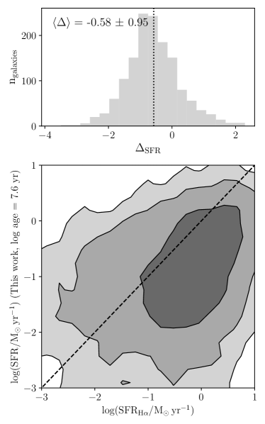
Figure A4: SFRs calculated for the sample galaxies in this work by using the STARLIGHT fitting procedure at a lookback time of $10^{7.6}\>\rm yr$ compared with SFRs derived from measurements of the $\rm H\alpha$ emission in these same galaxies. Similarly to Fig. A2, the lower plot shows confidence contours of $1\sigma$, $2\sigma$, and $3\sigma$ for the data, with the 1-to-1 relation shown by the dashed black diagonal line. The upper plot shows a histogram plotting the density distribution of the difference between the two measures of SFR, $\Delta_{\rm SFR}$. The mean value of this difference, $\langle\Delta\rangle$, and its standard deviation, are also shown in this upper plot.

Given the different systematic errors affecting these independent SFR estimates, a small offset is to be expected. This is a result also found by Peterken et al. (2021, see their Fig. 2), who also compared SFRs derived by STARLIGHT with $\rm SFR_{H\alpha}$ and found the latter quantity to be systematically slightly higher than the former. Such an offset will not, however, affect any of the conclusions presented in this paper. As such, we may conclude that the SFRs used in this work are – like the mass-weighted stellar metallicities produced by STARLIGHT – also indeed reasonably reliable and safe to use.

References

- Abdurro’uf et al. (2022) Abdurro’uf et al., 2022, ApJS, 259, 35
- Asa’d et al. (2017) Asa’d R. S., Vazdekis A., Cervino M., Noel N. E. D., Beasley M. A., Kassab M., 2017, MNRAS, 471, 3599
- Asplund et al. (2009) Asplund M., Grevesse N., Sauval A. J., Scott P., 2009, ARA&A, 47, 481
- Belfiore et al. (2019a) Belfiore F., et al., 2019a, AJ, 158, 160
- Belfiore et al. (2019b) Belfiore F., Vincenzo F., Maiolino R., Matteucci F., 2019b, MNRAS, 487, 456
- Bertelli et al. (1994) Bertelli G., Bressan A., Chiosi C., Fagotto F., Nasi E., 1994, A&AS, 106, 275
- Beverage et al. (2021) Beverage A. G., Kriek M., Conroy C., Bezanson R., Franx M., van der Wel A., 2021, ApJ, 917, L1
- Blanc et al. (2015) Blanc G. A., Kewley L., Vogt F. P., Dopita M. A., 2015, ApJ, 798, 99
- Blanton et al. (2011) Blanton M. R., Kazin E., Muna D., Weaver B. A., Price-Whelan A., 2011, AJ, 142, 31
- Blanton et al. (2017) Blanton M. R., et al., 2017, AJ, 154, 28
- Bresolin et al. (2006) Bresolin F., Pietrzynski G., Urbaneja M. A., Gieren W., Kudritzki R.-P., Venn K. A., 2006, ApJ, 648, 1007
- Brinchmann et al. (2004) Brinchmann J., Charlot S., White S. D. M., Tremonti C., Kauffmann G., Heckman T., Brinkmann J., 2004, MNRAS, 351, 1151
- Bundy et al. (2015) Bundy K., et al., 2015, ApJ, 798, 7
- Calzetti et al. (2000) Calzetti D., Armus L., Bohlin R. C., Kinney A. L., Koornneef J., Storchi-Bergmann T., 2000, ApJ, 533, 682
- Camps-Fariña et al. (2021) Camps-Fariña A., Sanchez S. F., Lacerda E. A. D., Carigi L., García-Benito R., Mast D., Galbany L., 2021, MNRAS, 504, 3478
- Camps-Fariña et al. (2022) Camps-Fariña A., et al., 2022, eprint (arXiv:2203.01159)
- Chabrier (2003) Chabrier G., 2003, PASP, 115, 763
- Cherinka et al. (2018) Cherinka B., et al., 2018, AJ, 158, 74
- Cid Fernandes (2018) Cid Fernandes R., 2018, MNRAS, 480, 4480
- Cid Fernandes & González Delgado (2010) Cid Fernandes R., González Delgado R. M., 2010, MNRAS, 403, 780
- Cid Fernandes et al. (2005) Cid Fernandes R., Mateus A., Sodré L., Stasińska G., Gomes J. M., 2005, MNRAS, 358, 363
- Cid Fernandes et al. (2014) Cid Fernandes R., et al., 2014, A&A, 561, A130
- Considère et al. (2000) Considère S., Coziol R., Contini T., Davoust E., 2000, A&A, 356, 89
- Cresci et al. (2019) Cresci G., Mannucci F., Curti M., 2019, A&A, 627, 42
- Croom et al. (2012) Croom S. M., et al., 2012, MNRAS, 421, 872
- Curti et al. (2020) Curti M., Mannucci F., Cresci G., Maiolino R., 2020, MNRAS, 491, 944
- Drory et al. (2015) Drory N., et al., 2015, AJ, 149, 77
- Fontanot et al. (2021) Fontanot F., et al., 2021, MNRAS, 504, 4481
- Fraser-McKelvie et al. (2022) Fraser-McKelvie A., et al., 2022, MNRAS, 510, 320
- Fu et al. (2012) Fu J., Kauffmann G., Li C., Guo Q., 2012, MNRAS, 424, 2701
- Gallazzi et al. (2005) Gallazzi A., Charlot S., Brinchmann J., White S. D., Tremonti C. A., 2005, MNRAS, 362, 41
- Ge et al. (2018) Ge J., Yan R., Cappellari M., Mao S., Li H., Lu Y., 2018, MNRAS, 478, 2633
- Girardi et al. (2000) Girardi L., Bressan A., Bertelli G., Chiosi C., 2000, A&AS, 141, 371
- Goddard et al. (2017) Goddard D., et al., 2017, MNRAS, 466, 4731
- González Delgado et al. (2014) González Delgado R. M., et al., 2014, ApJ, 791, 16
- Greener et al. (2020) Greener M. J., et al., 2020, MNRAS, 495, 2305
- Greener et al. (2021) Greener M. J., Merrifield M., Aragón-Salamanca A., Peterken T., Andrews B., Lane R. R., 2021, MNRAS, 502, L95
- Gunn et al. (2006) Gunn J. E., et al., 2006, AJ, 131, 2332
- Hägele et al. (2008) Hägele G. F., Díaz Á. I., Terlevich E., Terlevich R., Pérez-Montero E., Cardaci M. V., 2008, MNRAS, 383, 209
- Hart et al. (2016) Hart R. E., et al., 2016, MNRAS, 461, 3663
- Hart et al. (2017) Hart R. E., et al., 2017, MNRAS, 472, 2263
- Hunter (2007) Hunter J. D., 2007, Comput. Sci. Eng., 9, 90
- Kashino et al. (2016) Kashino D., Renzini A., Silverman J. D., Daddi E., 2016, ApJ, 823, L24
- Kashino et al. (2017) Kashino D., et al., 2017, ApJ, 835, 88
- Kashino et al. (2022) Kashino D., et al., 2022, ApJ, 925, 82
- Kennicutt (1998) Kennicutt R. C., 1998, ApJ, 498, 541
- Kewley & Dopita (2002) Kewley L. J., Dopita M. A., 2002, ApJS, 142, 35
- Kewley & Ellison (2008) Kewley L. J., Ellison S. L., 2008, ApJ, 681, 1183
- Kewley et al. (2006) Kewley L. J., Geller M. J., Barton E. J., 2006, AJ, 131, 2004
- Kewley et al. (2019) Kewley L. J., Nicholls D. C., Sutherland R. S., 2019, ARA&A, 57, 511
- Kobulnicky & Zaritsky (1999) Kobulnicky H. A., Zaritsky D., 1999, ApJ, 511, 118
- Lacerda et al. (2020) Lacerda E. A. D., Sánchez S. F., Cid Fernandes R., López-Cobá C., Espinosa-Ponce C., Galbany L., 2020, MNRAS, 492, 3073
- Lacerda et al. (2022) Lacerda E. A., Sánchez S., Mejía-Narváez A., Camps-Fariña A., Espinosa-Ponce C., Barrera-Ballesteros J., Ibarra-Medel H., Lugo-Aranda A., 2022, NewA, 97, 101895
- Lara-López et al. (2010) Lara-López M. A., et al., 2010, A&A, 521, 53
- Larson (1972) Larson R. B., 1972, Nature Phys. Sci., 236, 7
- Larson (1976) Larson R. B., 1976, MNRAS, 176, 31
- Law et al. (2015) Law D. R., et al., 2015, AJ, 150, 19
- Law et al. (2016) Law D. R., et al., 2016, AJ, 152, 83
- Lian et al. (2018a) Lian J., Thomas D., Maraston C., Goddard D., Comparat J., Gonzalez-Perez V., Ventura P., 2018a, MNRAS, 474, 1143
- Lian et al. (2018b) Lian J., Thomas D., Maraston C., 2018b, MNRAS, 481, 4000
- Madau & Dickinson (2014) Madau P., Dickinson M., 2014, ARA&A, 52, 415
- Madau et al. (1998) Madau P., Pozzetti L., Dickinson M., 1998, ApJ, 498, 106
- Maiolino & Mannucci (2019) Maiolino R., Mannucci F., 2019, A&A Rev., 27, 187
- Maiolino et al. (2008) Maiolino R., et al., 2008, A&A, 488, 463
- Mannucci et al. (2010) Mannucci F., Cresci G., Maiolino R., Marconi A., Gnerucci A., 2010, MNRAS, 408, 2115
- Mejía-Narváez et al. (2020) Mejía-Narváez A., Sánchez S. F., Lacerda E. A. D., Carigi L., Galbany L., Husemann B., García-Benito R., 2020, MNRAS, 499, 4838
- Moustakas et al. (2011) Moustakas J., et al., 2011, eprint (arXiv:1112.3300)
- Neumann et al. (2022) Neumann J., et al., 2022, MNRAS, 513, 5988
- Nicholls et al. (2017) Nicholls D. C., Sutherland R. S., Dopita M. A., Kewley L. J., Groves B. A., 2017, MNRAS, 466, 4403
- Noeske et al. (2007) Noeske K. G., et al., 2007, ApJ, 660, L43
- Onodera et al. (2015) Onodera M., et al., 2015, ApJ, 808, 161
- Paalvast & Brinchmann (2017) Paalvast M., Brinchmann J., 2017, MNRAS, 470, 1612
- Panter et al. (2008) Panter B., Jimenez R., Heavens A. F., Charlot S., 2008, MNRAS, 391, 1117
- Peterken et al. (2019) Peterken T., et al., 2019, MNRAS, 489, 1338
- Peterken et al. (2020) Peterken T., Merrifield M., Aragón-Salamanca A., Fraser-McKelvie A., Avila-Reese V., Riffel R., Knapen J., Drory N., 2020, MNRAS, 495, 3387
- Peterken et al. (2021) Peterken T., et al., 2021, MNRAS, 502, 3128
- Robitaille et al. (2013) Robitaille T. P., et al., 2013, A&A, 558
- Sánchez Almeida (2017) Sánchez Almeida J., 2017, ASSL, 430, 67
- Sánchez-Menguiano et al. (2019) Sánchez-Menguiano L., Almeida J. S., Muñoz-Tuñón C., Sánchez S. F., Filho M., Hwang H.-C., Drory N., 2019, ApJ, 882, 9
- Sánchez et al. (2012) Sánchez S. F., et al., 2012, A&A, 538, A8
- Sánchez et al. (2016a) Sánchez S. F., et al., 2016a, Rev. Mex. AA, 52, 21
- Sánchez et al. (2016b) Sánchez S. F., et al., 2016b, Rev. Mex. AA, 52, 171
- Sánchez et al. (2018) Sánchez S. F., et al., 2018, Rev. Mex. AA, 54, 217
- Sánchez et al. (2022) Sánchez S. F., et al., 2022, preprint (arXiv:2206.07062)
- Sanders et al. (2018) Sanders R. L., et al., 2018, ApJ, 858, 99
- Sanders et al. (2021) Sanders R. L., et al., 2021, ApJ, 914, 19
- Scudder et al. (2021) Scudder J. M., Ellison S. L., El Meddah El Idrissi L., Poetrodjojo H., 2021, MNRAS, 507, 2468
- Smee et al. (2013) Smee S. A., et al., 2013, AJ, 146, 32
- Somerville et al. (2015) Somerville R. S., Popping G., Trager S. C., 2015, MNRAS, 453, 4337
- Speagle et al. (2014) Speagle J. S., Steinhardt C. L., Capak P. L., Silverman J. D., 2014, ApJS, 214, 15
- Stasińska (2002) Stasińska G., 2002, Rev. Mex. AA conf. Ser., 12, 62
- Stasińska (2005) Stasińska G., 2005, A&A, 434, 507
- Talbot & Arnett (1971) Talbot R. J., Arnett W. D., 1971, ApJ, 170, 409
- Taylor (2005) Taylor M. B., 2005, Astronomical Data Analysis Software and Systems XIV - ASP Conference Series, 347, 29
- Telford et al. (2016) Telford O. G., Dalcanton J. J., Skillman E. D., Conroy C., 2016, ApJ, 827, 35
- Tinsley (1974) Tinsley B. M., 1974, ApJ, 192, 629
- Tinsley (1980) Tinsley B. M., 1980, Fund. Cosmic Phys., 5, 287
- Tremonti et al. (2004) Tremonti C. A., et al., 2004, ApJ, 613, 898
- Troncoso et al. (2014) Troncoso P., et al., 2014, A&A, 563, 58
- Vale Asari et al. (2007) Vale Asari N., Cid Fernandes R., Stasińska G., Torres-Papaqui J. P., Mateus A., Sodré L., Schoenell W., Gomes J. M., 2007, MNRAS, 381, 263
- Vale Asari et al. (2009) Vale Asari N., Stasinska G., Fernandes R. C., Gomes J. M., Schlickmann M., Mateus A., Schoenell W., 2009, MNRAS, 396, 71
- Vazdekis et al. (2010) Vazdekis A., Sánchez-Blázquez P., Falcón-Barroso J., Cenarro A. J., Beasley M. A., Cardiel N., Gorgas J., Peletier R. F., 2010, MNRAS, 404, 1639
- Vazdekis et al. (2016) Vazdekis A., Koleva M., Ricciardelli E., Röck B., Falcón-Barroso J., 2016, MNRAS, 463, 3409
- Virtanen et al. (2020) Virtanen P., et al., 2020, Nature Methods, 17, 261
- Wake et al. (2017) Wake D. A., et al., 2017, AJ, 154, 86
- Westfall et al. (2019) Westfall K. B., et al., 2019, AJ, 158, 231
- Whitaker et al. (2012) Whitaker K. E., van Dokkum P. G., Brammer G., Franx M., 2012, ApJ, 754, L29
- Wilkinson et al. (2017) Wilkinson D. M., Maraston C., Goddard D., Thomas D., Parikh T., 2017, MNRAS, 472, 4297
- Willett et al. (2013) Willett K. W., et al., 2013, MNRAS, 435, 2835
- Wuyts et al. (2014) Wuyts E., et al., 2014, ApJ, 789, 40
- Yabe et al. (2015) Yabe K., et al., 2015, PASJ, 67, 102
- Yan et al. (2016a) Yan R., et al., 2016a, AJ, 151, 8
- Yan et al. (2016b) Yan R., et al., 2016b, AJ, 152, 197
- Yates et al. (2012) Yates R. M., Kauffmann G., Guo Q., 2012, MNRAS, 422, 215
- Yates et al. (2021) Yates R. M., Henriques B. M. B., Fu J., Kauffmann G., Thomas P. A., Guo Q., White S. D. M., Schady P., 2021, MNRAS, 503, 4474
- Yi (2008) Yi S. K., 2008, ASP Conference Series, 392, 3
- Zahid et al. (2013a) Zahid H. J., Yates R. M., Kewley L. J., Kudritzki R.-P., 2013a, ApJ, 763, 92
- Zahid et al. (2013b) Zahid H. J., Geller M. J., Kewley L. J., Hwang H. S., Fabricant D. G., Kurtz M. J., 2013b, ApJ, 771, 19
- Zahid et al. (2014) Zahid H. J., Dima G. I., Kudritzki R. P., Kewley L. J., Geller M. J., Hwang H. S., Silverman J. D., Kashino D., 2014, ApJ, 791, 130
- Zahid et al. (2017) Zahid H. J., et al., 2017, ApJ, 847, 18
- Zhang et al. (2017) Zhang K., et al., 2017, MNRAS, 466, 3217
- Zhou et al. (2021) Zhou S., Li C., Hao C.-N., Guo R., Mo H., Xia X., 2021, ApJ, 916, 38
- Zhou et al. (2022) Zhou S., Merrifield M., Aragón-Salamanca A., 2022, MNRAS, 513, 5446
- van der Walt et al. (2011) van der Walt S., Colbert S. C., Varoquaux G., 2011, Comput. Sci. Eng., 13, 22