Reservoir-induced stabilisation of a periodically driven many-body system

Abstract

Exploiting the rich phenomenology of periodically-driven many-body systems is notoriously hindered by persistent heating in both the classical and quantum realm. Here, we investigate to what extent coupling to a large thermal reservoir makes stabilisation of a non-trivial steady state possible. To this end, we model both the system and the reservoir as classical spin chains where driving is applied through a rotating magnetic field, and simulate the Hamiltonian dynamics of this setup. We find that the intuitive limits of infinite and vanishing frequency, where the system dynamics is governed by the average and the instantaneous Hamiltonian, respectively, can be smoothly extended into entire regimes separated only by a small crossover region. At high frequencies, the driven system stroboscopically attains a Floquet-type Gibbs state at the reservoir temperature. At low frequencies, a synchronised Gibbs state emerges, whose temperature may depart significantly from that of the reservoir. Although our analysis in some parts relies on the specific properties our setup, we argue that much of its phenomenology should be generic for a large class of systems.

Introduction.–

Our understanding of periodically-driven quantum systems is largely facilitated by Floquet’s theorem Kitagawa-Oka-Brataas-Fu-Demler ; Sambe ; Torres-Kunold , which implies that the explicit time-dependence of Schrödinger’s equation can be removed by means of a unitary basis transformation with the same periodicity as the drive Bukov-DAlessio-Polkovnikov-review ; Eckardt-rmp . Hence, the stroboscopic time evolution of a such systems is generated by a time-independent Hermitian operator, the Floquet Hamiltonian, whose properties can be tailored through the applied driving protocol. This result opened the field of Floquet engineering Weitenberg-Simonet and led to the discovery of novel phenomena with no static counterpart such as anomalous Floquet topological insulators Rubio-Abadal ; Cayssol-Dora-Simon-Moessner or so-called time crystals Else-Bauer-Nayak ; vonKeyserlingk-Khemani-Sondhi ; Sacha-Zakrzewski .

The Floquet Hamiltonian of a many-body system is generally a complicated object, which in most cases can be determined only via approximate methods. Its eigenstates, which govern the long-time behaviour of the system, are generically superpositions of its instantaneous energy eigenstates with quasi-homogeneously distributed coefficients Moessner-Sondhi ; Zhang-Khemani-Huse . Combining this observation with the notion that energy eigenstates typically display thermal behaviour, i.e. the eigenstate thermalisation hypothesis Deutsch ; Srednicki ; Rigol-Dunjko-Olshanii ; DAlessio-Kafri-Polkovnikov-Rigol , leads to an ensemble with no conservation laws DAlessio-Rigol ; Kim-Ikeda-Huse . That is, a generic many-body system continuously absorbs energy until the statistics of all observables are described by a structureless infinite-temperature ensemble Ponte-Chandran-Papic-Abanin ; Russomanno-Silva-Santoro ; Kuwahara-Mori-Saito ; Abanin-DeRoeck-Huveneers . In practice, this behaviour confines Floquet engineering to the high-frequency regime, where heating is exponentially suppressed, or to special systems where thermalisation is hindered by other means such as many-body localisation Fleckenstein-Bukov ; Ishii-Kuwahara-Mori-Hatano ; BAA ; Nandkishore-Huse ; vonKeyserlingk-Sondhi .

Floquet theory does not apply to systems obeying non-linear dynamics. A variety of techniques used in analysing periodically driven quantum systems such as high-frequency expansions may, however, be naturally adopted in a classical Hamiltonian framework Bukov-DAlessio-Polkovnikov-review and much phenomenology may persist.

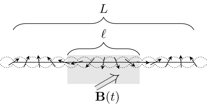
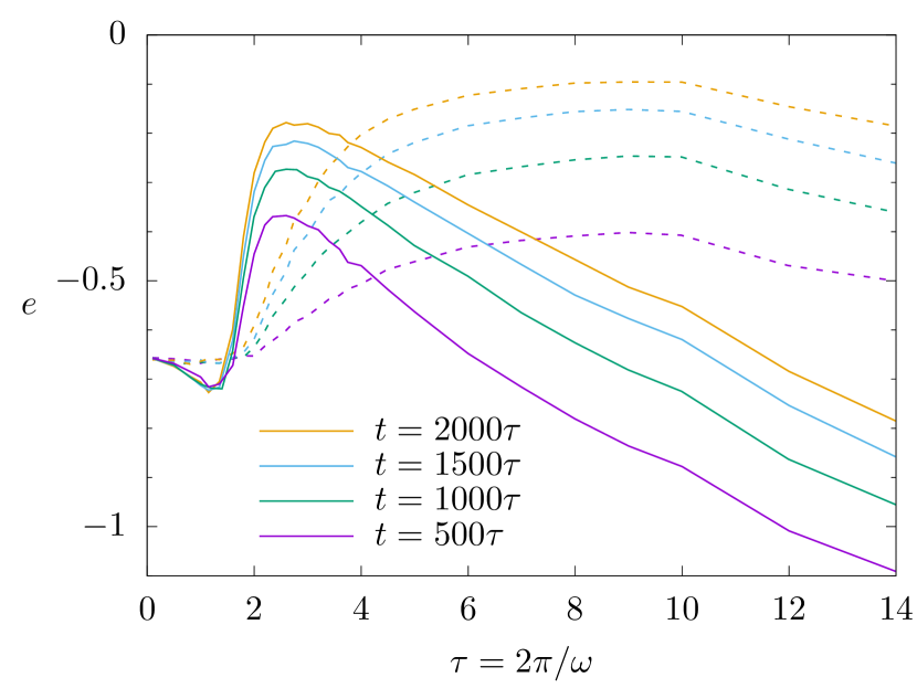
Figure 1: Above: Sketch of the system. A classical spin chain with nearest-neighbour interactions, wark disorder, and total number of sites $L$, $\ell$ of which are exposed to a time-periodic magnetic field ${\bf B}(t)$. Below: Mean energy density of the driven system as a function of the period $\tau$ over the elapsed time $t$. While nearly no energy is absorbed for $\tau\lesssim 2$, a reservoir-stabilised steady state with strongly suppressed absorption emerges for $\tau\gtrsim 3$, before heating eventually prevails due to finite-size effects (solid, $L=2000$). By contrast, the isolated system rapidly heats up for $\tau\gtrsim 2$ (dashed, $L=\ell$). For all plots we have set $\ell=20$, $\delta J=2\times 10^{-2}$, $e_{\rm initial}=-0.66$, see main text for symbols.

Nonetheless, systematic investigations of classical systems have begun only recently, despite greater numerical accessibility of larger systems sizes and longer evolution times than in the quantum case Nunnenkamp ; Howell ; Mori-Floquet-prethermal ; Citro-Dalla-Torre ; Bukov-DAlessio-Polkovnikov-review ; McRoberts-Bilitewski-Haque-Moessner . Here, we exploit this advantage to explore reservoir-induced thermalisation as a new approach to avoid overheating in periodically driven many-body systems.

For concreteness, we consider a classical spin chain with a magnetic drive applied to a finite region, and the remainder of the system acting as a reservoir, see Fig. 1. At high driving frequencies, the system is well-described by the time-averaged Hamiltonian, up to perturbative corrections in the inverse driving frequency; this behaviour is qualitatively insensitive to the presence of the reservoir. In the quasi-static limit, the system relaxes to the instantaneous Hamiltonian before it changes appreciably. At any finite frequency, however, the existence and nature of a stroboscopic steady state is a priori unclear. Our main finding is that the reservoir stabilises a non-trivial steady state over a wide range of frequencies and on an intermediate but practically long timescale, where the isolated system would overheat, see Fig. 1. This steady state, which is smoothly connected to the quasi-static limit, emerges through synchronisation between the driven system and the reservoir, suppressing net energy absorption long-paper , and is described by a Gibbs ensemble whose temperature can deviate significantly from the initial temperature of the reservoir. This behaviour is in clear contrast with the intuitive expectation of the reservoir acting as a mere energy sink, whose state is invariant up to finite-size corrections. In the following, we explicitly construct both high- and low-frequency ensembles, which describe all local observables of the driven system, leaving only a small crossover region unexplained by a steady state.

Setup.–

We consider the setup of Fig. 1. We will refer to the $\ell$ driven sites as the system proper, and the remaining $L-\ell$ sites of the spin-chain as the reservoir, where we are particularly interested in the regime $\ell\ll L$. The dynamical variables are classical spin vectors normalised such that $|{\bf S}_{j}|^{2}=1$. The Hamiltonian of the entire system is

$$H(t)=-\sum_{j=1}^{L}{\bf S}_{j}^{\top}J_{j}{\bf S}_{j+1}+\sum_{j=1}^{\ell}{\bf B}(t)\cdot{\bf S}_{j}.$$ (1)

We assume periodic boundary conditions i.e. ${\bf S}_{L+1}={\bf S}_{1}$. The $J_{j}$ are diagonal matrices whose entries $J_{j}^{\alpha}$ are independently and identically distributed and drawn from a normal distribution with mean $J=1$, which we use as our energy scale throughout, and variance $\delta J$. The driving ${\bf B}(t)=J(\cos\omega t,\sin\omega t,0)^{\top}$ is a rotating planar magnetic field with period $\tau=2\pi/\omega$. We choose $\delta J$ small but non-zero to ensure that there are no conserved quantities, which would constrain the dynamics.

The time evolution of the system is determined by Hamilton’s equations of motion, $\frac{\mathrm{d}f}{\mathrm{d}t}=\frac{\partial f}{\partial t}+\{f,H\}$, where the Poisson bracket for spin degrees of freedom is determined by the Lie algebra of $SO(3)$

$$\{S_{j}^{\alpha},S_{k}^{\beta}\}=\delta_{jk}\varepsilon^{\alpha\beta\gamma}S_{j}^{\gamma}.$$ (2)

Accordingly, the microscopic equations of motion are

$$\frac{\mathrm{d}{\bf S}_{j}}{\mathrm{d}t} =-{\boldsymbol{\Omega}}_{j}\times{\bf S}_{j},$$ (3)

$${\boldsymbol{\Omega}}_{j} =J_{j-1}{\bf S}_{j-1}+J_{j}{\bf S}_{j+1}-\begin{cases}{\bf B}(t)&1\leq j\leq\ell\\ 0&\ell<j\leq L\end{cases}.$$

We choose our initial state as a global equilibrium state with zero magnetic field. Initial conditions are sampled using standard Metropolis-Hastings Monte Carlo (MC) methods from the Gibbs distribution

$$P_{0}(\{{\bf S}_{j}\})=e^{-\beta H_{0}}/Z_{0}$$ (4)

with $H_{0}=-\sum_{j=1}^{L}{\bf S}_{j}^{\top}J_{j}{\bf S}_{j+1}$ Newman-Barkema . Throughout this article, $P$ will denote a probability density and $Z$ a normalisation constant. The dynamics are numerically realised via symplectic integration which manifestly conserves spin-normalisation Krech-Bunker-Landau . Unless otherwise stated, presented results are averages over a large number of initial states and disorder realisations. We confirm in Ref. [long-paper, ] that in the absence of driving and with small $\delta J=10^{-3}$, time and ensemble averages are indeed equivalent i.e. the free system is ergodic.

We first explore the existence of a steady-state through observables of the system proper, specifically focusing on magnetisation and energy density, given by

$${\bf m} =\frac{1}{\ell}\sum_{j=1}^{\ell}{\bf S}_{j},$$ (5)

$$e =-\frac{1}{\ell-1}\sum_{j=1}^{\ell-1}{\bf S}_{j}^{\top}J_{j}{\bf S}_{j+1}+{\bf m}\cdot{\bf B}(t).$$

The energy of the system proper is a salient observable through which to explore reservoir-induced stabilisation. In Fig. 1, we plot the stroboscopic energy density $e(t=n\tau)$ after a large number of cycles $n$, where we set $\delta J=0.02$ such that heating is observable on the timescales considered. To gain a clearer theoretical picture of the different regimes, we henceforth take $\delta J=10^{-3}$ in order to increase the separation of timescales between heating and relaxation to the intermediate steady state.

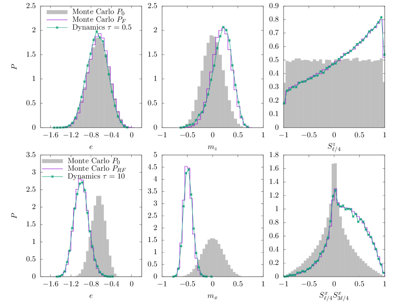
Figure 2: Probability density histograms of stroboscopic observables for dynamical evolution and statistical descriptions, $\ell=20$, $L=2000$, $\delta J=10^{-3}$, $\beta$ chosen such that $e_{\rm initial}=-0.66$. Here $e$, $m_{x}$, $m_{z}$, and $m_{x}$ are determined by Eq. (5), $S^{z}_{\ell/4}$ is the $z$-component of the spin at site $j=\ell/4$, and $S^{x}_{\ell/4}S^{x}_{3\ell/4}$ is the product of the $x$-components of the spins at sites $j=\ell/4$ and $j=3\ell/4$, highlighting that spatial correlations are also captured by the stroboscopic low-frequency ensemble of Eq. (11). For comparison, the initial ensemble $P_{0}$ of Eq. (4) is shown in grey. Top: fast-driving regime, $\tau=0.5$, purple curves show MC sampling of from Eq. (7) with $\beta_{F}=\beta$, dynamics sampled at $t=2000\tau$. Bottom: slow-driving regime, $\tau=10$, where purple curves show MC sampling of from Eq. (11) with $\beta_{RF}$ determined from Eq. (12), and dynamics are sampled at $t=1000\tau$.

High-frequency regime.–

When the system is driven at a frequency $\omega\gg J$ we expect its physics to be well-approximated by the time-averaged Hamiltonian, with corrections scaling as powers of $\omega^{-1}$, given by the classical Floquet-Magnus expansion Oteo-Ros ; Blanes-Casas-Oteo-Ros ; large-omega-comment ; Bukov-DAlessio-Polkovnikov-review . Note that we formally set $\hbar=1$ such that the spins are dimensionless and energies and inverse timescales have the same dimension. Such expansions are generally asymptotic in $\omega^{-1}$ and only in special cases is resummation possible feldman . More precisely, rigorous recent results on the classical limit of quantum spin-chains demonstrate that the Floquet-Magnus Hamiltonian approximates a conserved quantity as $\omega\to\infty$, although the stroboscopic evolution of observables generated by $H_{F}$ is not guaranteed to converge to those of the true time-dependent evolution Mori-Kuwahara-Saito-prl-2016 . In our case, the leading order gives the Floquet Hamiltonian

$$H_{F}^{(1)}=-\sum_{j=1}^{L}{\bf S}_{j}^{\top}J^{HF}_{j}{\bf S}_{j+1}-\frac{J^{2}}{2\omega}\sum_{j=1}^{\ell}{\bf\hat{z}}\cdot{\bf S}_{j}+\mathcal{O}(\omega^{-2})$$ (6)

with the modified couplings $J^{HF}_{j}=Q_{j}^{\top}J_{j}Q_{j+1}$, where $Q_{j}=R_{y}(J/\omega)$ represents rotation around the $y$-axis by $J/\omega$ for $j=1,\ldots,\ell$ and the identity otherwise Bukov-DAlessio-Polkovnikov-review .

In the absence of other conserved quantities, statistical-mechanics leads us to posit a stroboscopic Floquet-Gibbs ensemble of the form

$$P_{F}(\{{\bf S}_{j}\})=e^{-\beta_{F}H_{F}}/Z_{F},$$ (7)

where $H_{F}$ is an appropriately truncated Floquet-Magnus expansion. For our purposes, we find it sufficient to set $H_{F}=H_{F}^{(1)}$ Floquet-gibbs-1 ; Floquet-gibbs-2 . As $\omega\gg J$, energy absorption is significantly suppressed, and we expect that the effective inverse temperature fulfills $\beta_{F}\approx\beta$. Fig. 2 shows that such an ensemble reproduces the statistics of system proper observables well for $\tau=0.5$, where the leading correction in $\omega^{-1}$ is necessary to capture the asymmetry in observables involving $S^{z}_{j}$. We confirm in Ref. [long-paper, ] that higher-order corrections can indeed be safely neglected.

Low-frequency regime.–

We observe that our model admits an almost-static description in the rotating frame defined by introducing new variables ${\bf S}_{j}=R(t)\widetilde{\bf S}_{j}$, where

$$R(t)=\begin{pmatrix}\cos(\omega t)&-\sin(\omega t)&0\\ \sin(\omega t)&\cos(\omega t)&0\\ 0&0&1\end{pmatrix}.$$ (8)

The microscopic equations of motion become

$$\frac{\mathrm{d}\widetilde{\bf S}_{j}}{\mathrm{d}t} =-\widetilde{\boldsymbol{\Omega}}_{j}\times\widetilde{\bf S}_{j}+\mathcal{O}(\delta J)=\{\widetilde{\bf S}_{j},H_{RF}\}+\mathcal{O}(\delta J),$$ (9)

$$\widetilde{\boldsymbol{\Omega}}_{j} =J\widetilde{\bf S}_{j-1}+J\widetilde{\bf S}_{j+1}+\begin{cases}\omega\hat{\bf z}-J\hat{\bf x}&1\leq j\leq\ell\\ \omega\hat{\bf z}&\ell<j\leq L\end{cases}.$$

Here, we have neglected time-dependent corrections of order $\delta J$ and introduce the rotating-frame Hamiltonian

$$H_{RF}=-\sum_{j=1}^{L}\left[\widetilde{\bf S}_{j}\cdot\widetilde{\bf S}_{j+1}+\omega\hat{\bf z}\cdot\widetilde{\bf S}_{j}\right]+\sum_{j=1}^{\ell}\hat{\bf x}\cdot\widetilde{\bf S}_{j}.$$ (10)

Since the transformation (8) reduces to the identity at every integer multiple of the period, the autonomous dynamics generated by $H_{RF}$ are stroboscopically equivalent to the dynamics of the drive system in the limit $\delta J\ll J$.

In this global Floquet picture, statistical mechanics implies that the total system should, after some transient phase, be stroboscopically described by a canonical ensemble

$$P_{RF}(\{{\bf S}_{j}\})=e^{-\beta_{RF}H_{RF}}/Z_{RF},$$ (11)

where $\beta_{RF}$ is an effective inverse temperature. Two remarks are in order here. First, although we neglect order $\delta J$ corrections to the rotating-frame Hamiltonian, which can be calculated systematically by means of a Floquet-Magnus expansion long-paper , we still assume that the disorder makes the system ergodic. Second, as the total system is closed, one would in principle have to use a micro-canonical ensemble in Eq. (11). However, here we prefer the technically simpler canonical ensemble, which should be equivalent for any local observables if $L\gg 1$.

On a timescale slower than the inverse heating rate $H_{RF}$ is approximately conserved, and so the Lagrange multiplier $\beta_{RF}$ may be fixed by requiring that the expectation value of $H_{RF}$ in the final ensemble of Eq. (11) is the same as in the initial ensemble of Eq. (4) i.e.

$$\int\mathrm{d}{\bf S}_{1}\dots\mathrm{d}{\bf S}_{L}H_{RF}(\{{\bf S}_{j}\})e^{-\beta H_{0}(\{{\bf S}_{j}\})}/Z_{0}=$$ (12)

$$\ \int\mathrm{d}{\bf S}_{1}\dots\mathrm{d}{\bf S}_{L}H_{RF}(\{{\bf S}_{j}\})e^{-\beta_{RF}H_{RF}(\{{\bf S}_{j}\})}/Z_{RF}.$$

In the limit $L\gg\ell$, these quantities are dominated by the reservoir terms and become independent of $\ell$. Thus Eq. (12) implicitly defines an effective reservoir temperature $\beta_{RF}=\beta_{RF}(\beta,\omega)$, which may be found numerically using MC methods. We recover instantaneous equilibration in the quasi-static limit i.e. $\lim_{\omega\to 0}\beta_{RF}(\beta,\omega)=\beta$.

We show in Fig. 2 that the ensemble of Eq. (11) convincingly reproduces dynamical results after 1000 cycles. Fruthermore, the mean energy density derived from Eq. (12) agrees well with the dynamics for $\tau\gtrsim 5$, see Fig. 3. These results underpin our main insight: at low and intermediate frequencies, although being applied only locally, the driving gradually affects the entire system as the reservoir synchronises with the system proper and an equilibrium state with low net energy absorption emerges long-paper . This collective behaviour, which is mediated only by short-range interactions, is in stark contrast with the conventional notion of a thermal reservoir as a reversible heat sink, which is realised here only in the high-frequency regime.

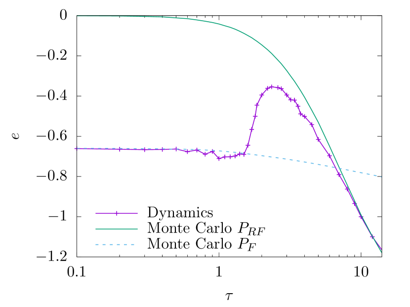
Figure 3: Energy of the system proper from dynamical simulations and ensemble descriptions of Eq. (7) with $\beta_{F}=\beta$ (high frequency), and Eq. (11) (low frequency), with $\beta_{RF}$ determined from Eq. (12). We have set $e_{\rm initial}=-0.66$, $\ell=20$, $L=2000$, $t=1000\tau$, $\delta J=10^{-3}$.

Perspectives.–

Our results provide strong evidence that effective equilibrium states may be stroboscopically established in a periodically driven open many-body system over a wide range of frequencies. The limits $\omega\to 0$ and $\omega\to\infty$ match physical intuition, and we have demonstrated that even leading-order correction in $\omega^{-1}$ and $\omega$ respectively are sufficient to account for all but a small frequency window around $\tau\approx 2$. This crossover regime may still be described by a non-equilibrium steady state featuring persistent currents. A natural mechanism for generating such currents would be an emerging phase lag in the synchronisation that governs the low-frequency regime. Hence, an increasing inability of the system to respond to the drive could be the physical origin for the breakdown of the low-frequency ensemble which, on dimensional grounds, must occur at $\omega/J\sim 1$.

The existence of a rotating frame is contingent on our choice of the drive. We nonetheless generically expect relaxation to an instantaneous Gibbs ensemble in the quasi-static limit $\omega\to 0$. The instantaneous Hamiltonian then plays the role of an adiabatic invariant, and it would be interesting to pursue a perturbative construction of analogous invariants away from this limit. Although numerically accessible, the analytic construction of such ensembles is likely not straightforward. However, by numerically evaluating the response functions entering fluctuation-dissipation relations, it is in principle possible to verify that a system is in equilibrium without specific knowledge of its state.

There remain many interesting questions about the relationship between the convergence of the high-frequency expansions and heating and the role of effective conservation laws. In addition, it would be instructive to explore how the physics that we have uncovered here survives or is modified in higher dimensions, where the same theoretical manipulations are in principle possible.

Data access statement.–

The source code used for all simulations, and all data used in figures, is freely available at https://github.com/tveness/spinchain-papers.

References

- (1) T. Kitagawa, T. Oka, A. Brataas, L. Fu, E. Demler, Phys. Rev. B 84, 235108 (2011).
- (2) H. Sambe, Phys. Rev. A 7, 2203 (1973).
- (3) M. Torres and A. Kunold, Phys. Rev. B 71, 115313 (2005).
- (4) M. Bukov, L. D’Alessio, A. Polkovnikov, Adv. Phys. 64, 139 (2015).
- (5) A. Eckardt, Rev. Mod. Phys. 89, 011004 (2017).
- (6) C. Weitenberg, J. Simonet, Nat. Phys. 17, 1342 (2021).
- (7) A. Rubio-Abadal, M. Ippoliti, S. Hollerith, D. Wei, J. Rui, S. L. Sondhi, V. Khemani, C. Gross, I. Bloch, Phys. Rev. X 10, 021044 (2020).
- (8) J. Cayssol, B. Dóra, F. Simon, R. Moessner, Phys. Stat. Sol. RRL 7, 101 (2013).
- (9) D. V. Else, B. Bauer, C. Nayak, Phys. Rev. Lett. 117, 090402 (2016).
- (10) C. W. von Keyserlingk, V. Khemani, S. L. Sondhi, Phys. Rev. B 94, 085112 (2016).
- (11) K. Sacha, J. Zakrzewski, Rep. Prog. Phys. 81, 016401 (2017).
- (12) R. Moessner, S. L. Sondhi, Nat. Phys. 13, 424 (2017).
- (13) L. Zhang, V. Khemani, D. A. Huse, Phys. Rev. B 94, 224202 (2016).
- (14) J. M. Deutsch, Phys. Rev. A 43, 2046 (1991).
- (15) M. Srednicki, Phys. Rev. E 50, 888 (1994).
- (16) M. Rigol, V. Dunjko, M. Olshanii, Nature 452, 854 (2008).
- (17) L. D’Alessio, Y. Kafri, A. Polkovnikov, M. Rigol, Adv. Phys. 65, 239 (2016).
- (18) L. D’Alessio, M. Rigol, Phys. Rev. X 4, 041048 (2014).
- (19) H. Kim, T. N. Ikeda, D. A. Huse, Phys. Rev. E 90, 052105 (2014).
- (20) P. Ponte, A. Chandran, Z. Papic, D. A. Abanin, Ann. Phys. 353, 196 (2015).
- (21) A. Russomanno, A. Silva, G. E. Santoro, J. Stat. Mech. P09012 (2013).
- (22) T. Kuwahara, T. Mori, K. Saito, Ann. Phys. 367, 96 (2016).
- (23) D. A. Abanin, W. De Roeck, F. Huveneers, Phys. Rev. Lett. 115 256803l (2015).
- (24) C. Fleckenstein, M. Bukov, Phys. Rev. B 103, 144307 (2021).
- (25) T. Ishii, T. Kuwahara, T. Mori, N. Hatano, Phys. Rev. Lett. 120, 220602 (2018).
- (26) D. Basko, I. Aleiner, B. Altshuler, Ann. Phys. 321, 1126 (2006).
- (27) R. Nandkishore, D. A. Huse, Ann. Rev. Condens. Matter Phys. 6, 15 (2015).
- (28) C. W. von Keyserlingk, S. L. Sondhi, Phys. Rev. B 93, 245146 (2016).
- (29) T. Veness, K. Brandner, Reservoir-induced stabilisation of a periodically driven classical spin chain: local vs. global relaxation (2022).
- (30) M. E. J. Newman, G. T. Barkema, Monte Carlo methods in statistical physics, Clarendon Press (1999).
- (31) M. Krech, A. Bunker, D. P. Landau, Comput. Phys. Comm. 111, 1 (1998).
- (32) A. J. McRoberts, T. Bilitewski, M. Haque, R. Moessner, Phys. Rev. B 105, L100403 (2022).
- (33) A. Pizzi, A. Nunnenkamp, J. Knolle, Phys. Rev. Lett. 127, 140602 (2021).
- (34) O. Howell, P. Weinberg, D. Sels, A. Polkovnikov, M. Bukov, Phys. Rev. Lett. 122, 010602 (2019).
- (35) T. Mori, Phys. Rev. B 98, 104303 (2018).
- (36) R. Citro, E. G. Dalla Torre, L. D’Alessio, A. Polkovnikov, M. Babadi, T. Oka, E. Demler, Ann. Phys. 360, 694 (2015).
- (37) J. A. Oteo, J. Ros, J. Phys. A 24, 5751 (1991).
- (38) S. Blanes, F. Casas, J. A. Oteo, J. Ros, Phys. Rep. 470, 151 (2009).
- (39) Other methods yield identical results to leading order, including continuous averaging Guckenheimer-Holmes ; Kapitsa and the method of multiple scales Bender-Orszag
- (40) J. Guckenheimer, P. Holmes, Nonlinear oscillations, dynamical systems, and bifurcations of vector fields (Vol. 42), Springer Science & Business Media (2013).
- (41) L. D. Landau, E. M. Lifshitz, Mechanics. Vol. 1 §30, Pergamon Press (1960)
- (42) C. M. Bender, S. Orszag, Advanced mathematical methods for scientists and engineers I: Asymptotic methods and perturbation theory (Vol. 1), Springer Science & Business Media (1999).
- (43) E. B. Fel’dman, Phys. Lett. A 104 (1984).
- (44) T. Mori, T. Kuwahara, K. Saito, Phys. Rev. Lett. 116, 120401 (2016).
- (45) T. Shirai, J. Thingna, T. Mori, S. Denisov, P. Hänggi, S. Miyashita, New J. Phys. 18, 053088 (2016).
- (46) T. Shirai, T. Mori, S. Miyashita, Eur. Phys. J. Special Topics 227, 323 (2018).