A framework for implementing general virtual element spaces

Abstract

In this paper we present a framework for the construction and implementation of general virtual element spaces based on projections built from constrained least squares problems. Building on the triples used for finite element spaces, we introduce the concept of a VEM tuple which encodes the necessary building blocks to construct these projections. Using this approach, a wide range of virtual element spaces can be defined. We discuss $H^{k}$-conforming spaces for $k=1,2$ as well as divergence and curl free spaces. This general framework has the advantage of being easily integrated into any existing finite element package and we demonstrate this within the open source software package Dune.

65M60, 65N30, 65Y15, 65-04

1 Introduction

In recent years research and development of the virtual element method (VEM) has skyrocketed. The method, which was introduced in [11], is an extension of the finite element method (FEM) and has many benefits. These include, but are not limited to, the handling of general polytopal meshes as well as the construction of spaces with additional structure such as arbitrary global regularity [7, 15]. The method is highly flexible and as such has been applied to a wide range of problems. The list is extensive and detailing all developments goes beyond the scope of this paper, an overview can be found in [4].

One of the main ideas behind the virtual element method is that the basis functions are considered virtual and do not need to be evaluated explicitly. In contrast to standard FEM, the local spaces may include functions which are not polynomials. Therefore, when setting up the stiffness matrix there are additional procedures which need to be carried out as projection operators need to be introduced and used when one of the entries of the stiffness matrix is a non-polynomial. It is important to stress that the computation of the projections is the only modification required to switch between a finite element and a virtual element discretisation.

A key part of the virtual element method is the construction of the aforementioned projection operators which are necessary to construct the discrete bilinear form. Usually, one projection operator is built which depends on the local contribution of the bilinear form [11]. This approach leads to some restrictions as for example it does not extend easily to nonlinear problems or to PDEs with non-constant coefficients. Also, it is not straightforward to integrate such a method into an existing finite element package which relies on the spaces not depending on the data of the PDE being solved. An alternative approach first introduced in [1] and extended to general second-order elliptic problems in [20], involves a VEM enhancement technique to ensure the computation of certain $L^{2}$-projections. This approach was extended to fourth-order problems in [26] and applied to a nonlinear example in [25] where the starting point for the construction of projections is a constrained least squares (CLS) problem.

We aim to generalise this projection approach even further by introducing a general VEM framework in which we describe how to define fully computable projections starting from what we call a generic VEM tuple. The VEM tuple should be thought of as an extension of the well known finite element triple $(E,\mathcal{P}^{E},\Lambda^{E})$ [22]. Under the assumption of unisolvency of $\Lambda^{E}=\{\lambda_{1}^{E},\dots,\lambda_{N}^{E}\}$, this triple provides all the information required to construct the nodal basis functions $\Phi^{E}=\{\phi_{1}^{E},\dots,\phi_{N}^{E}\}$, i.e. a basis of $\mathcal{P}^{E}$ satisfying $\lambda_{i}^{E}(\phi^{E}_{j})=\delta_{ij}$. Code to evaluate the basis functions $\Phi^{E}$ and their derivatives for a given FEM triple forms the fundamental building block of most finite element packages. In most cases changing the element type, the properties of the spaces, or even only the order of the method can lead to a considerable amount of new code. Implementing more specialised finite element spaces is often so cumbersome that few software packages provide these spaces. For example, spaces to handle fourth-order problems in primal form are often not available except sometimes in the form of the lowest order nonconforming Morley element [35].

The introduction of a VEM tuple in this paper aims to extend the idea of a FEM triple as a fundamental building block for the implementation of a wide variety of VEM spaces. In particular, we incorporate all of the information required to build the projection operators in the VEM tuple. One of the benefits of this generic approach is the ability to build spaces with additional properties. We showcase this through examples detailing how to construct $H^{k}$-conforming for $k=1,2$, nonconforming, curl free and divergence free spaces suitable for e.g. acoustic vibration problems [16], Stokes flow [14, 23], to name but a few.

Extending the FEM concepts i.e. replacing the evaluation of the nodal basis functions and their derivatives with the evaluation of projection operators, reduces the complexity of adding virtual element methods to existing software frameworks. Such frameworks include for example deal.II [9], DUNE [10], Feel++ [37], FEniCS [2], Firedrake [38], or FreeFEM++ [30]. This is in contrast to available VEM software implementations such as [31, 33, 36, 40] which are often highly restrictive in what they offer. Either only lowest order spaces are available or there is no functionality to solve nonlinear problems. In this paper we explain the steps necessary to adapt a finite element implementation to include virtual element spaces. As proof of concept we demonstrate in two space dimensions how to integrate our general framework into a finite element package using the Dune-Fem module which is a part of the Dune software framework [28]. Switching between a finite element and a virtual element discretisation is seamless for users due to the Dune Python frontend. To the best of our knowledge, this is the first implementation of the virtual element method within a large finite element software package to include spaces suitable for nonlinear problems in addition to spaces with the extra properties listed above.

The paper is organised as follows. In Section 2 we detail the notation and state the model problem followed by the details of the discretised problem. The abstract virtual element framework is outlined in Section 3 including the construction of the projection operators from a given VEM tuple. In Section 3.4 we provide a number of VEM tuples suitable for a wide range of different problems. We restrict the main presentation to second-order problems in two space dimensions but provide an overview in Section 4 of how the framework extends to fourth-order problems and in Section 5 we sketch the extension of the approach to three space dimensions. We outline how to use the general framework to add VEM spaces to existing FEM software packages in Section 6. Finally, numerical experiments are presented in Section 7. Note that for now our proof of concept implementation is restricted to two space dimensions.

2 Problem setup

In this preliminary section we describe the notation and setup a model problem which we will use as an example during the discussion of the general concepts in the following.

2.1 Mesh notation and assumptions

Let $\mathcal{T}_{h}$ denote a tessellation of a domain $\Omega\subset\mathbb{R}^{d}$ for $d=2,3$, where $\Omega$ is a polygonal domain in 2D and a polyhedral domain in 3D. We assume the tessellation is made up of simple polygonal or polyhedral elements which do not overlap. Moreover, we assume that the boundary of each element is made up of a uniformly bounded number of interfaces (edges in 2D and faces in 3D) where each boundary is either part of $\partial\Omega$ or shared with another element in $\mathcal{T}_{h}$. We denote an element in $\mathcal{T}_{h}$ by $E$ with $h_{E}:=\text{diam}(E)$, and let $h$ denote the maximum of the diameters over all elements in $\mathcal{T}_{h}$. We denote with $s$ a $(d-1)$-dimensional mesh interface, either an edge when $d=2$ or a face when $d=3$. The set of all interfaces in the mesh is denoted by $\mathcal{S}_{h}$. For $E\in\mathcal{T}_{h}$ we denote by $\mathcal{S}_{h}(E)$ the set of all mesh interfaces which are part of $E$, i.e., $\mathcal{S}_{h}(E):=\{s\in\mathcal{S}_{h}:s\subset\partial E\}$.

We denote the space of polynomials over $E\in\mathcal{T}_{h}$ with degree up to and including $\ell\in\mathbb{N}$ by $\mathbb{P}_{\ell}(E)$. We also require a hierarchical basis for $\mathbb{P}_{\ell}(E)$, which we denote by $\mathcal{M}_{\ell}(E)$. An example is given by scaled monomials which are defined as follows. Firstly, for $k\in\mathbb{N}$, we denote by $\mathcal{M}^{*}_{k}(E)$ the scaled monomials of order $k$

$$\mathcal{M}^{*}_{k}(E)=\left\{\left(\frac{x-x_{E}}{h_{E}}\right)^{\alpha}\text{ with }\alpha\in\mathbb{N}^{d},\,|\alpha|=k\right\}$$

where $x_{E}$ denotes the barycentre of $E\in\mathcal{T}_{h}$, and $\alpha$ represents a multi-index with $|\alpha|=\sum_{i=1}^{d}\alpha_{i}$. Then, we take as basis of $\mathbb{P}_{\ell}(E)$ the set $\mathcal{M}_{\ell}(E)$ where

(2.1) $$\mathcal{M}_{\ell}(E):=\cup_{k\leq\ell}\mathcal{M}^{*}_{k}(E).$$

Notice that we can also construct bases for polynomial spaces defined on interfaces $s$ in the same way denoted with $\mathcal{M}_{\ell}(s)$.

2.2 Model problem and discrete setup

From now on, we restrict the presentation of the framework to two space dimensions, i.e. let $\Omega\subset\mathbb{R}^{2}$ denote a polygonal domain. We begin by setting up the model problem and describe the corresponding discrete problem. Note that we introduce the model problem with purposeful ambiguity to demonstrate the wide range of problems our framework can be applied to. To this end, assume that we have a form $a(\cdot,\cdot)$ defined on $V\times V$, where $V$ is the function space in which we define the associated PDE. We assume $a(\cdot,\cdot)$ can be expressed in the following way

(2.2) $$a(v,w)=\sum_{E\in\mathcal{T}_{h}}a^{E}(v,w)~{},\;a^{E}(v,w)=\int_{E}D(v,\nabla v)\cdot\nabla w\,\mathrm{d}x+\int_{E}m(v,\nabla v)w\,\mathrm{d}x$$

for some possibly nonlinear $D,m$. Further, for a linear functional $L$ defined on $V$, we assume that there exists a unique solution $u\in V$ such that

(2.3) $$a(u,v)={\color[rgb]{0,0,0}L(v)}\quad\forall v\in V.$$

Since we introduce a model problem with deliberate ambiguity, alongside the abstract concepts, we also introduce a running example in the simplest setting. That is, we make use of the two-dimensional Laplace problem in order to demonstrate the ideas behind our framework which are introduced throughout this section.

Example 2.1 (Conforming VEM example in 2D).

For a polygonal $\Omega\subset\mathbb{R}^{2}$, consider the following two-dimensional Laplace problem for some $f\in L^{2}(\Omega)$:

$$-\Delta u ={\color[rgb]{0,0,0}f},\quad \text{ in }\Omega,$$

with homogeneous Dirichlet boundary conditions. Therefore, to fit into the above format, we take the space ${V=H^{1}_{0}(\Omega)}$ and to obtain the bilinear form $a(\cdot,\cdot)$, we take $D(u,\nabla u)=\nabla u$ and $m$ to be zero. This gives $a(u,v)=(\nabla u,\nabla v)$, together with $L(v)=(f,v)$ it is clear that (2.3) has a unique solution via the Lax-Milgram lemma.

Remark 2.2.

We point out that we can include vector valued problems with a form $a(\cdot,\cdot):\boldsymbol{V}\times\boldsymbol{V}\rightarrow\mathbb{R}$, where $\boldsymbol{V}:=[V]^{r}$ for some $r>1$ and could for example be taken as $\boldsymbol{V}:=[H^{1}_{0}(\Omega)]^{r}$ in the case that $a(\boldsymbol{v},\boldsymbol{w}):=(\nabla\boldsymbol{v},\nabla\boldsymbol{w})$.

Next, given a space $\widetilde{V}$ not necessarily satisfying $\widetilde{V}\subset V$, we define a discrete bilinear form $a_{h}:\widetilde{V}\times\widetilde{V}\rightarrow\mathbb{R}$ such that for any $v_{h},w_{h}\in\widetilde{V}$

$$a_{h}(v_{h},w_{h})=\sum_{E\in\mathcal{T}_{h}}a_{h}^{E}(v_{h},w_{h})$$

where $a_{h}^{E}:\widetilde{V}|_{E}\times\widetilde{V}|_{E}\rightarrow\mathbb{R}$ is the restriction of the bilinear form $a_{h}$ to an element $E$. Denote this restriction of $\widetilde{V}$ to an element $E$ by $\widetilde{V}^{E}$. We assume further that the discrete form has the following form

(2.4) $$\begin{split}a_{h}^{E}(v_{h},w_{h})=&\int_{E}D(\Pi^{E}_{0}v_{h},\Pi^{E}_{1}v_{h})\cdot\Pi^{E}_{1}w_{h}\,\mathrm{d}x+\int_{E}m(\Pi^{E}_{0}v_{h},\Pi^{E}_{1}v_{h})\Pi^{E}_{0}w_{h}\,\mathrm{d}x\\ &+{\color[rgb]{0,0,0}(\bar{D}+\bar{m}h_{E}^{2})}S^{E}(v_{h}-\Pi^{E}_{0}v_{h},w_{h}-\Pi^{E}_{0}w_{h})\end{split}$$

for any $v_{h},w_{h}\in\widetilde{V}^{E}$, where $D,m$ have been given in Eq. 2.2, and $\bar{D}$, $\bar{m}$ are constants necessary to achieve the right scaling of the so called VEM stabilisation form $S^{E}(\cdot,\cdot)$. $S^{E}(\cdot,\cdot)$ denotes a symmetric, positive definite bilinear form necessary to ensure the coercivity of $a_{h}^{E}(\cdot,\cdot)$. Furthermore, $\Pi^{E}_{\mu}$ denotes a value projection for $\mu=0$ and a gradient projection for $\mu=1$ chosen so that

(2.5) $$\Pi^{E}_{\mu}v_{h}\sim\nabla^{\mu}v_{h}|_{E},\quad\mu=0,1.$$

In order to discretise the right hand side of (2.3), for any $v_{h}\in\widetilde{V}$ we define $L_{h}(v_{h}):=\sum_{E\in\mathcal{T}_{h}}L_{h}^{E}(v_{h})$. In the case of Example 2.1, we define $L^{E}_{h}(v_{h}):=(f,\Pi^{E}_{0}v_{h})_{E}$, i.e. we utilise the value projection. Note that for the remainder of this paper we focus on the bilinear form. In particular, the definitions of the projections will be made precise in the virtual element setting in Section 3.

Remark 2.3.

For a classical conforming FEM discretisation we would simply take $S^{E}=0$ and $\Pi^{E}_{\mu}v_{h}=\nabla^{\mu}v_{h}|_{E}$ so that $a_{h}^{E}(v_{h},w_{h})={\color[rgb]{0,0,0}a^{E}}(v_{h},w_{h})$ and $L_{h}^{E}(v_{h})=L^{E}(v_{h})=(f,v_{h})_{E}$.

Definition 2.4 (Degrees of freedom).

For $E\in\mathcal{T}_{h}$, we define a set of degrees of freedom (dof set) $\Lambda^{E}$ as a set of functionals $\lambda:\widetilde{V}\rightarrow\mathbb{R}$.

For a given dof set $\Lambda^{E}$ we define the subset $\Lambda^{E,s}$ for $s\in\mathcal{S}_{h}(E)$ as follows

(2.6) $$\Lambda^{E,s} :=\{\lambda\in\Lambda^{E}:\ \lambda(v^{E})=\lambda(w^{E})\text{ if }v^{E}|_{\bar{s}}=w^{E}|_{\bar{s}}\}.$$

We assume the following.

1. The dof set $\Lambda^{E}$ is unisolvent, i.e., a function $v_{h}$ in the local discrete space is uniquely determined by its degrees of freedom (dofs).

2. The dofs depend only on values of $v_{h}$ but not on derivatives.

3. The polynomial space is a subset of the local discrete VEM space, where $\ell$ represents a positive integer.

Note that (A2) will be generalised in a later section (Section 4) when we consider fourth-order problems. We now give an example set of dofs for Example 2.1.

As considered in e.g. [11, 20], for a polygon $E\in\mathcal{T}_{h}$, we consider the set of dofs $\Lambda^{E}$ for the $H^{1}$-conforming VEM. For $\ell\geq 1$, we define the following dofs.

1. • The values of $v_{h}$ for each vertex of $E$.

   • For $\ell>1$, the moments of $v_{h}$ up to order $\ell-2$ on each edge $s\in\mathcal{S}_{h}(E)$,

     (2.7) $$\frac{1}{|s|}\int_{s}v_{h}m_{\ell-2}\,\mathrm{d}s\quad \forall m_{\ell-2}\in\mathcal{M}_{\ell-2}(s).$$

2. For $\ell>1$, the moments of $v_{h}$ up to order $\ell-2$ inside the element $E$

   $$\frac{1}{|E|}\int_{E}v_{h}m_{\ell-2}\,\mathrm{d}x\quad \forall m_{\ell-2}\in\mathcal{M}_{\ell-2}(E).$$

In this example, we have $N^{s}+N^{s}(\ell-1)+\frac{1}{2}\ell(\ell-1)$ total dofs where $N^{s}$ denotes the number of edges in the polygon $E$. The dof set $\Lambda^{E,s}$ contains the dofs in (a), that is, the two dofs $v_{h}(s^{\pm})$ where $s^{\pm}$ denotes the vertices attached to the edge $s$, as well as the $|\mathcal{M}_{\ell-2}(s)|=\ell-1$ edge dofs.

Key to the virtual element discretisation is the concept of computability which we capture in the next definition.

Definition 2.5 (Computable).

Given $F\in\mathcal{T}_{h}$ (or ${F\in\mathcal{S}_{h}(E)}$ for some $E\in\mathcal{T}_{h}$), we say that a quantity is computable from $\Lambda^{F}$ (or $\Lambda^{E,s}$) if it is a linear combination of $\lambda\in\Lambda^{F}(\text{ or }\Lambda^{E,s})$.

3 Abstract virtual element framework

In this section we introduce an approach to construct general VEM spaces based on ideas borrowed from the abstract FEM framework where a triple is used to define the local space. We begin by defining the VEM tuple before describing the projection framework in two space dimensions. Recall that the projections are necessary to construct the discrete form (2.4). In particular, the element value projection $\Pi^{E}_{0}$ and gradient projection $\Pi^{E}_{1}$ are chosen so that they are as “close” as possible to the true value and gradient operators (2.5).

Within the projection framework we introduce two value projections, one for each element $E\in\mathcal{T}_{h}$ and one for each edge $s\in\mathcal{S}_{h}(E)$. These value projections are defined as solutions of a constrained least squares problem with the constraint set specified by the VEM tuple. The projections for the higher order derivatives e.g. the gradient or hessian projections are then defined hierarchically using these projections, independent of the space. We discuss the gradient projection here since we are focusing on second-order problems and delay the description of the generic construction of the hessian projection to Section 4.

3.1 Virtual element tuple

The starting point for the general framework is the notion of a virtual element tuple. The tuple contains all of the building blocks for the computation of the projection operators.

Definition 3.1 (Virtual element tuple).

We define a virtual element tuple $\mathcal{V}^{F}$

(3.1) $$\mathcal{V}^{F}={(F,\mathcal{B}_{0}^{F},\Lambda^{F},\mathcal{C}^{F}_{0},\mathcal{B}_{1}^{F})}$$

consisting of the following.

• A mesh object $F$ with either $F\in\mathcal{T}_{h}$ or $F\in\mathcal{S}_{h}$.

• A basis set $\mathcal{B}_{0}^{F}$ used for a value projection e.g. a subset of $[\mathcal{M}_{\ell}(F)]^{r}$ (see Eq. 2.1), where $r=1$ for scalar and $r>1$ for vector valued spaces, $|\mathcal{B}_{0}^{F}|\leq|\Lambda^{F}|$, and when $F\in\mathcal{T}_{h}$, $\mathcal{B}_{0}^{F}$ is a subset of the local discrete VEM space.

• A set of dofs $\Lambda^{F}$ subject to the conditions in Section 2.2.

• A set of linear functionals $\mathcal{C}^{F}_{0}$ computable from $\Lambda^{F}$. These will be called constraints in the following.

• When $F\in\mathcal{T}_{h}$, a basis set $\mathcal{B}_{1}^{F}$ used for a gradient projection. Note that since the basis set $\mathcal{B}_{1}^{F}$ is used to construct the gradient projection, it must at least be a vector valued quantity, e.g. a subset of $[\mathcal{M}_{\ell-1}(F)]^{r\times 2}$.

For the set of VEM tuples $(\mathcal{V}^{E})_{E\in\mathcal{T}_{h}}$ and $(\mathcal{V}^{s})_{s\in\mathcal{S}_{h}}$ we say that the VEM tuples are compatible if $\Lambda^{s}\subset\Lambda^{E}$ whenever $s\in\mathcal{S}_{h}(E)$.

For our conforming VEM running example, the dof set $\Lambda^{E}$ is taken as those described previously in Example 2.1(a)-(b). For each $E\in\mathcal{T}_{h}$, we take as basis set the monomial basis $\mathcal{B}_{0}^{E}$ from Eq. 2.1 of order $\ell$ and we take the basis for the gradient projection, $\mathcal{B}_{1}^{E}$, to be the monomials of order $\ell-1$, i.e. $\mathcal{B}_{1}^{E}:=[\mathcal{M}_{\ell-1}(E)]^{2}$. Also, for this example, for each $s\in\mathcal{S}_{h}(E)$, we take $\mathcal{B}_{0}^{s}$ to be $\mathcal{M}_{\ell}(s)$. That is, we shall define the value projections such that $\Pi^{E}_{0}v_{h}\in$ and $\Pi^{s}_{0}v_{h}\in$. Furthermore, we shall define the gradient projection such that $\Pi^{E}_{1}v_{h}\in[$. The dof set for the edge tuple is taken to be $\Lambda^{s}:=\Lambda^{E,s}$. We will discuss the constraints sets $\mathcal{C}^{E}_{0},\mathcal{C}^{s}_{0}$ for this example later in this section.

For the remainder of this section we now fix $E\in\mathcal{T}_{h}$ and $\Lambda^{E}$. In order to ensure compatibility of the VEM tuples we take $\Lambda^{s}:=\Lambda^{E,s}$ which is defined in Eq. 2.6 for $s\in\mathcal{S}_{h}(E)$. Then it is clear that $\Lambda^{s}\subset\Lambda^{E}$.

Remark 3.2.

For second-order elliptic problems, when $F\in\mathcal{S}_{h}(E)$ the basis set $\mathcal{B}_{1}^{F}$ is not prescribed as we do not require higher order derivative projections on the edges, this is due to (A2). The more general case will be discussed later.

Remark 3.3.

To construct finite element spaces a triple of the form $(F,\mathcal{B}_{0}^{F},\Lambda^{F})$ is commonly used. The main difference to the VEM tuple is that in the FEM setting $\mathcal{B}_{0}^{F}$ is a basis of the local space, in fact usually the local space itself is used in the FEM triple. In our VEM framework, we can have $|\mathcal{B}_{0}^{E}|<N^{E}$ where $N^{E}$ denotes the dimension of the discrete space. So only a (mostly polynomial) subspace of the local space is specified by the VEM tuple.

Both the basis sets $\mathcal{B}^{F}_{\mu}$ for $\mu=0,1$ and the constraint set $\mathcal{C}^{F}_{0}$ are kept ambiguous to allow for the construction of VEM spaces with different properties. In Section 3.4 we give concrete examples for these choices, but in general the basis sets will be sets of monomials used as a basis for various polynomial spaces.

3.2 Gradient projection

We now give the details of the projection framework. Given an element $E\in\mathcal{T}_{h}$, attached edges, and VEM tuples $\mathcal{V}^{E}$, $\mathcal{V}^{s}$ (see Definition 3.1) we introduce value projections $\Pi^{E}_{0},$ $\Pi^{s}_{0}$ for each edge $s$, and a gradient projection $\Pi^{E}_{1}$. In order to illustrate the hierarchical construction process, we start by giving the definition of the gradient projection in terms of the value projections $\Pi^{E}_{0}$, $\Pi^{s}_{0}$ to be determined later. The definition of the gradient projection comes from an application of integration by parts followed by a replacement of the lower order terms with computable projections, as shown in the next definition. This ensures that the gradient projection is fully computable. Note that it is more usual in the VEM literature to first define the gradient projection and then to use that to define the value projection.

Definition 3.4 (Gradient projection).

For a discrete function $v_{h}$ and an element $E\in\mathcal{T}_{h}$, we define the gradient projection $\Pi^{E}_{1}$ into the span of the basis set $\mathcal{B}_{1}^{E}$, where $\mathcal{B}_{1}^{E}$ is provided by the VEM tuple $\mathcal{V}^{E}$ (3.1). Then for any $v_{h}\in\widetilde{V}^{E}$, $\Pi^{E}_{1}$ satisfies

$$\int_{E}\Pi^{E}_{1}v_{h}\cdot q\,\mathrm{d}x=-\int_{E}\Pi^{E}_{0}v_{h}\nabla\cdot q\,\mathrm{d}x+\sum_{s\in\mathcal{S}_{h}(E)}\int_{s}\Pi^{s}_{0}v_{h}(n\cdot q)\,\mathrm{d}s$$

for all $q\in\mathcal{B}_{1}^{E}$, where $n$ denotes the outward pointing normal to the edge $s$.

Motivated by this definition, it is clear why we need to construct an inner value projection and projections on each edge $s\in\mathcal{S}_{h}(E)$.

3.3 Value projections

In this section, we now let $F$ denote either the element $E$ or an edge $s\in\mathcal{S}_{h}(E)$. We stress that there is no difference in the construction of the value projection whether $F$ is an element or an edge. Either way, these projections are defined using a constrained least squares problem, which we assume is uniquely solvable. Details on how to implement this projection can be found in Section 6 where we also discuss the unique solvability of the constrained least squares problem.

Definition 3.5 (Value projection).

For a discrete function $v_{h}$, we define the value projection $\Pi^{F}_{0}$ into the span of the basis set $\mathcal{B}_{0}^{F}$, where $\mathcal{B}_{0}^{F}$ is provided by $\mathcal{V}^{F}$. We define the value projection $\Pi^{F}_{0}$ as the solution to the following CLS problem

$${\rm min}\sum_{\lambda\in\Lambda^{F}}(\lambda(\Pi^{F}_{0}v_{h}-v_{h}))^{2},\qquad\text{subject to}\quad\mathcal{C}(\Pi^{F}_{0}v_{h}-v_{h})=0\quad\forall\mathcal{C}\in\mathcal{C}^{F}_{0}.$$

We revisit Example 2.1 again, giving concrete examples for the constraint set choices in the VEM tuples for this example.

We have so far defined all components of the VEM tuple except the constraint sets. One important aim of the constraints is to make sure that the value projection is an $L^{2}$ projection into as large a polynomial set as possible. Consequently, if for some polynomial $q$ the right hand side $\int_{E}v_{h}q$ of the $L^{2}$ projection of a discrete function $v_{h}$ is computable from its degrees of freedom, then the value projection should be constrained to satisfy $\int_{E}\Pi^{F}_{0}v_{h}q=\int_{E}v_{h}q$. In the case of the $H^{1}$-conforming space with dofs given by Example 2.1(a)-(b), we therefore take as constraint set a scalar multiple of the inner moments:

(3.2) $$\mathcal{C}(v_{h}):=\int_{E}v_{h}m_{\ell-2}\,\mathrm{d}x,\quad m_{\ell-2}\in\mathcal{M}_{\ell-2}(E).$$

The constraint set for the edges is given by the edge dofs only from Eq. 2.7. This leads to the following CLS problem for the value projection on each edge with a unique solution in .

(3.3) $${\rm min}\sum_{\lambda\in\Lambda^{s}}(\lambda(\Pi^{s}_{0}v_{h}-v_{h}))^{2}\quad\text{subject to}\int_{s}\left(\Pi^{s}_{0}v_{h}-v_{h}\right)m_{\ell-2}\,\mathrm{d}s=0,\ m_{\ell-2}\in\mathcal{M}_{\ell-2}(s).$$

Remark 3.6.

We note that for the upcoming $H^{1}$-conforming and nonconforming examples we can show using the standard approach of “extended VEM spaces” as in [20, 26] that for any discrete $v_{h}$ and for $\mu=0,1$

$$\Pi^{E}_{\mu}v_{h}=\mathcal{P}^{E}_{\ell-\mu}(\nabla^{\mu}v_{h}).$$

This says that the value projection is indeed the $L^{2}$-projection, denoted by $\mathcal{P}^{E}_{p}$ for $p\in\mathbb{N}$, and the gradient projection is the $L^{2}$-projection of the gradient. This follows due to our choice of constraints, combined with the standard “extended VEM space” approach. We therefore obtain the usual $L^{2}$ property necessary for convergence analysis.

3.4 Examples

In this section we give concrete examples of VEM tuples for specific problems. Our generic framework allows us to build further VEM spaces with additional properties and a unified way to construct the projection operators for these problems. It is important to reiterate that assuming we are given $E\in\mathcal{T}_{h}$ and $\Lambda^{E}$, when $s\in\mathcal{S}_{h}(E)$ we take $\Lambda^{s}:=\Lambda^{E,s}$ in the VEM tuple $\mathcal{V}^{s}$. Recall that $\Lambda^{E,s}$ is defined in Eq. 2.6 and satisfies $\Lambda^{E,s}\subset\Lambda^{E}$ thus ensuring compatibility of the VEM tuples.

3.4.1 Example: $H^{1}$-conforming VEM

We summarise the VEM tuple for the $H^{1}$-conforming VEM in two dimensions from the running Example 3.3 in Table 1.

Table 1: VEM tuple summary for the $H^{1}$-conforming VEM in two dimensions. We introduce $q\in\mathbb{N}$ with $q\leq\ell$ for the gradient basis set $\mathcal{B}_{1}^{E}$.

$\mathcal{B}_{0}^{E}$	$\Lambda^{E}$	$\mathcal{C}^{E}_{0}$	$\mathcal{B}_{1}^{E}$	$\mathcal{B}_{0}^{s}$	$\mathcal{C}^{s}_{0}$
$\mathcal{M}_{\ell}(E)$	Example 2.1(a)-(b)	Eq. 3.2	$[\mathcal{M}_{q}(E)]^{2}$	$\mathcal{M}_{\ell}(s)$	Eq. 3.3

Remark 3.7 (Stabilisation free spaces).

As discussed in Example 3.1, the natural choice for $q$ in Table 1 for the gradient basis set $\mathcal{B}_{1}^{E}$ is $q:=\ell-1$ however, we can take $q:=\ell$ following ideas for stabilisation free VEM as introduced for the lowest order space in [17].

Remark 3.8.

Another choice of basis set for the gradient projection which is smaller than $[\mathcal{M}_{\ell-1}(E)]^{2}$ could be $\mathcal{B}_{1}^{E}:=\nabla\mathcal{M}_{\ell}(E)$. This choice of basis set is suitable for constant coefficient problems as otherwise it leads to suboptimal convergence rates for varying coefficients as remarked in [13].

Remark 3.9 (Serendipity spaces).

The serendipity approach discussed in [12] can be easily incorporated by choosing fewer moment degrees of freedom in the interior of each element without needing a change to the projection operators.

3.4.2 Example: $H^{1}$-nonconforming VEM

In this example we consider a nonconforming VEM space suitable for second-order problems taking the degrees of freedom considered in e.g. [20, 21, 8].

Definition 3.10.

For $\ell\geq 1$, we define the following dofs.

• The moments of $v_{h}$ up to order $\ell-1$ on each edge $s\in\mathcal{S}_{h}(E)$

  (3.4) $$\frac{1}{|s|}\int_{s}v_{h}m_{\ell-1}\,\mathrm{d}s\quad \forall m_{\ell-1}\in\mathcal{M}_{\ell-1}(s).$$

• For $\ell>1$, the moments of $v_{h}$ up to order $\ell-2$ inside the element $E$

  (3.5) $$\frac{1}{|E|}\int_{E}v_{h}m_{\ell-2}\,\mathrm{d}x\quad \forall m_{\ell-2}\in\mathcal{M}_{\ell-2}(E).$$

Note that the set $\Lambda^{E,s}\subset\Lambda^{E}$ includes the dofs in Eq. 3.4 for each $s\in\mathcal{S}_{h}(E)$. The constraints for the edge value projection are a scalar multiple of the edge moments described in Eq. 3.4. Each constraint is therefore of the form

(3.6) $$\mathcal{C}(v_{h}):=\int_{s}v_{h}m_{\ell-1}\,\mathrm{d}s,\quad m_{\ell-1}\in\mathcal{M}_{\ell-1}(s).$$

Table 2 summarises the choices for the other quantities of the VEM tuple.

Table 2: VEM tuples for the nonconforming VEM. In particular, we define the value projection into $\text{Span}(\mathcal{M}_{\ell}(E))=$ and the edge projections into $\text{Span}(\mathcal{M}_{\ell-1}(s))=$.

$\mathcal{B}_{0}^{E}$	$\Lambda^{E}$	$\mathcal{C}^{E}_{0}$	$\mathcal{B}_{1}^{E}$	$\mathcal{B}_{0}^{s}$	$\mathcal{C}^{s}_{0}$
$\mathcal{M}_{\ell}(E)$	Definition 3.10	Eq. 3.2	$[\mathcal{M}_{q}(E)]^{2}$	$\mathcal{M}_{\ell-1}(s)$	Eq. 3.6

Similarly to Remark 3.7, the natural choice is $q:=\ell-1$ however in the spirit of [17] we can also take $q:=\ell$ for a stabilisation free VEM for this nonconforming example.

Remark 3.11.

The main difference to the conforming case is that $\Pi^{s}_{0}$ is only into . This is sufficient for computing the gradient projection which only requires moments in $\mathcal{B}_{1}^{E}=[\mathcal{M}_{\ell-1}(E)]^{2}$ to be exact.

3.4.3 Example: Divergence free VEM

For this example we present the projection approach in the divergence free setting based on the reduced dof set described in [14].

Definition 3.12.

For $\ell\geq 2$, we define the following dofs for a discrete vector field $\boldsymbol{v}_{h}$.

• The values of $\boldsymbol{v}_{h}$ for each vertex of $E$.

• The moments up to order $\ell-2$ for each edge $s\in\mathcal{S}_{h}(E)$,

  $$\frac{1}{|s|}\int_{s}\boldsymbol{v}_{h}\cdot\boldsymbol{m}_{\ell-2}\,\mathrm{d}s\quad \forall\boldsymbol{m}_{\ell-2}\in[\mathcal{M}_{\ell-2}(s)]^{2}.$$

• The moments of $\boldsymbol{v}_{h}$ inside the element $E$

  $$\frac{1}{|E|}\int_{E}\boldsymbol{v}_{h}\cdot\boldsymbol{m}_{\ell-2}^{\perp}\,\mathrm{d}x\quad \forall\boldsymbol{m}_{\ell-2}^{\perp}\in\boldsymbol{x}^{\perp}[\mathcal{M}_{\ell-3}(E)],$$

with the notation $\boldsymbol{x}^{\perp}:=(x_{2},-x_{1})$.

For this example we also assume as in [14] that each discrete function in the local VEM space satisfies $\nabla\cdot\boldsymbol{v}_{h}\in$ and $\boldsymbol{v}_{h}|_{s}\in[$ for each $s\in\mathcal{S}_{h}(E)$. This allows us to show important properties of the projections.

Up until now we have always taken the element constraint set $\mathcal{C}_{0}^{E}$ to contain the inner dofs. However, in this example we take some additional constraints as well as the inner dofs.

(3.7) $$\mathcal{C}(\boldsymbol{v}_{h}) :=\int_{E}\boldsymbol{v}_{h}\cdot\boldsymbol{m}_{\ell-2}^{\perp}\,\mathrm{d}x,\quad\boldsymbol{m}_{\ell-2}^{\perp}\in\boldsymbol{x}^{\perp}[\mathcal{M}_{\ell-3}(E)],$$

and in addition

(3.8) $$\mathcal{C}(\boldsymbol{v}_{h}) :=\int_{E}\boldsymbol{v}_{h}\cdot\nabla m_{\ell-1}\,\mathrm{d}x,\quad m_{\ell-1}\in\mathcal{M}_{\ell-1}(E)\backslash\mathcal{M}_{0}(E).$$

The constraints for the edge value projection are the vector version of those used in the $H^{1}$-conforming example and so we are able to define $\Pi^{s}_{0}\boldsymbol{v}_{h}\in[$. Since we assume $\boldsymbol{v}_{h}|_{s}\in[$, it follows that $\Pi^{s}_{0}\boldsymbol{v}_{h}=\boldsymbol{v}_{h}|_{s}$.

Note that the constraints in Eq. 3.8 are indeed computable and necessary to show properties of the discrete space - see Remark 3.13. Computability follows from applying integration by parts to the right hand side,

$$\int_{E}\boldsymbol{v}_{h}\cdot\nabla m_{\ell-1}\,\mathrm{d}x =-\int_{E}\nabla\cdot\boldsymbol{v}_{h}m_{\ell-1}\,\mathrm{d}x+\sum_{s\in\mathcal{S}_{h}(E)}\int_{s}(\boldsymbol{v}_{h}\cdot\boldsymbol{n})m_{\ell-1}\,\mathrm{d}s.$$

Assuming that $m_{\ell-1}$ is in an orthonormal basis, the first term disappears due to the assumption $\nabla\cdot\boldsymbol{v}_{h}\in$. The boundary term can also be computed using the edge projection since $\boldsymbol{v}_{h}|_{s}\in[$.

We now have all the ingredients to provide the VEM tuple given in Table 3.

Table 3: VEM tuples for the divergence free VEM. Notice that this example is vector valued and as such the basis set for the element value projection is $[\mathcal{M}_{\ell}(E)]^{2}$.

$\mathcal{B}_{0}^{E}$	$\Lambda^{E}$	$\mathcal{C}^{E}_{0}$	$\mathcal{B}_{1}^{E}$	$\mathcal{B}_{0}^{s}$	$\mathcal{C}^{s}_{0}$
$[\mathcal{M}_{\ell}(E)]^{2}$	Definition 3.12	Eq. 3.7-Eq. 3.8	$[\mathcal{M}_{\ell-1}(E)]^{2\times 2}$	$[\mathcal{M}_{\ell}(s)]^{2}$	Eq. 3.3

Remark 3.13.

Using integration by parts, the constraints in Eq. 3.8, and the exactness of the edge projection, we can show that $\text{tr}(\Pi^{E}_{1}v_{h})\in$. In particular, for any test function $m_{\beta}\in\mathcal{M}_{\ell-1}(E)\backslash\mathcal{M}_{0}(E)$ it holds that

$$\int_{E}\text{tr}(\Pi^{E}_{1}\boldsymbol{v}_{h})m_{\beta}\,\mathrm{d}x =-\int_{E}\Pi^{E}_{0}\boldsymbol{v}_{h}\cdot\nabla m_{\beta}\,\mathrm{d}x+\sum_{s\in\mathcal{S}_{h}(E)}\int_{s}(\Pi^{s}_{0}\boldsymbol{v}_{h}\cdot\boldsymbol{n})m_{\beta}\,\mathrm{d}s$$

$$=\int_{E}(\nabla\cdot\boldsymbol{v}_{h})m_{\beta}\,\mathrm{d}x.$$

From an implementation perspective, this property is highly valuable as it is one possibile approach which avoids the construction of additional projection operators for the divergence. We implement the divergence directly as the trace of the gradient projection which is likely to be the default implementation available in a finite-element code.

3.4.4 Example: Curl free VEM

We now show how our generic approach can be applied to construct a curl free space using the dof set considered for an acoustic vibration problem in [16].

Definition 3.14.

For $\ell\geq 0$, we define dofs for a vector field $\boldsymbol{v}_{h}$:

• The moments up to order $\ell$ for each edge $s\in\mathcal{S}_{h}(E)$,

  (3.9) $$\frac{1}{|s|}\int_{s}(\boldsymbol{v}_{h}\cdot\boldsymbol{n})m_{\ell}\,\mathrm{d}s\quad \forall m_{\ell}\in\mathcal{M}_{\ell}(s).$$

• The moments of $\boldsymbol{v}_{h}$ inside the element $E$,

  (3.10) $$\frac{1}{\sqrt{|E|}}\int_{E}\boldsymbol{v}_{h}\cdot\nabla m_{\ell}\,\mathrm{d}x\quad \forall m_{\ell}\in\mathcal{M}_{\ell}(E)\backslash\mathcal{M}_{0}(E).$$

As in [16], for this example we assume further that discrete functions in the local VEM space satisfy $\nabla\cdot\boldsymbol{v}_{h}\in$ and $(\boldsymbol{v}_{h}\cdot\boldsymbol{n})\in$ for each $s\in\mathcal{S}_{h}(E)$.

As in the previous example, we take as constraints the inner dofs as well as additional constraints based on the additional property $\nabla\cdot v_{h}\in$. They are of the following form.

(3.11) $$\mathcal{C}(\boldsymbol{v}_{h}) :=\int_{E}\boldsymbol{v}_{h}\cdot\nabla m_{\ell}\,\mathrm{d}x, m_{\ell}\in\mathcal{M}_{\ell}(E),$$

(3.12) $$\mathcal{C}(\boldsymbol{v}_{h}) :=\int_{E}\boldsymbol{v}_{h}\cdot\nabla m_{\ell+1}\,\mathrm{d}x, m_{\ell+1}\in\mathcal{M}_{\ell+1}(E)\backslash\mathcal{M}_{\ell}(E).$$

The constraints for the edge value projection are again a scalar multiple of the edge dofs in Eq. 3.9 and, for any $s\in\mathcal{S}_{h}(E)$, are of the form

(3.13) $${\color[rgb]{0,0,0}\int_{s}\boldsymbol{v}_{h}\cdot\boldsymbol{m_{\ell}}\,\mathrm{d}s,\quad\boldsymbol{m_{\ell}}\in\boldsymbol{n}\mathcal{M}_{\ell}(s).}$$

These constraints allows us to define the edge projection into and therefore $\Pi^{s}_{0}\boldsymbol{v}_{h}=\boldsymbol{v}_{h}|_{s}$.

It is clear that the constraints in Eq. 3.11 are computable using the dofs whereas the constraints in Eq. 3.12 reduce to the following

$$\int_{E}\boldsymbol{v}_{h}\cdot\nabla m_{\ell+1}\,\mathrm{d}x =-\int_{E}\nabla\cdot\boldsymbol{v}_{h}m_{\ell+1}\,\mathrm{d}x+\sum_{s\in\mathcal{S}_{h}(E)}\int_{s}(\boldsymbol{v}_{h}\cdot\boldsymbol{n})m_{\ell+1}\,\mathrm{d}s.$$

Assuming that we have an orthonormal basis for , the first term vanishes since we have $\nabla\cdot\boldsymbol{v}_{h}\in$. The boundary terms are also computable using the edge projection. The VEM tuples for this example are summarised in Table 4.

Table 4: VEM tuple summary for the curl free example. We use $I_{2\times 2}$ to denote the identity matrix in $\mathbb{R}^{2}$.

$\mathcal{B}_{0}^{E}$	$\Lambda^{E}$	$\mathcal{C}^{E}_{0}$	$\mathcal{B}_{1}^{E}$	$\mathcal{B}_{0}^{s}$	$\mathcal{C}^{s}_{0}$
$\nabla\mathcal{M}_{\ell+1}(E)$	Definition 3.14	Eq. 3.11-Eq. 3.12	$\mathcal{M}_{\ell}(E)I_{2\times 2}$	$\mathcal{M}_{\ell}(s)\boldsymbol{n}$	Eq. 3.13

Remark 3.15.

Similarly to Remark 3.13, we can show ${\rm tr}(\Pi^{E}_{1}v_{h})\in$. The projections are curl free due to the choice of basis sets $\mathcal{B}_{0}^{E}:=\nabla\mathcal{M}_{\ell+1}(E)$ and ${\mathcal{B}_{1}^{E}:=\mathcal{M}_{\ell}(E)I_{2\times 2}}$.

4 Extension to fourth-order problems

In this section we show how to generalise our framework to include fourth-order problems. We restrict our extension of the generic framework to the $H^{2}$-conforming and nonconforming VEM spaces considered in [7, 19] and [6, 26, 41], respectively. Additional nonconforming spaces which can be constructed using the concepts discussed in this paper were analysed and tested in [26]. These are especially suited for solving fourth-order perturbation problems.

4.1 Hessian projection

Since we are now considering biharmonic-type problems, we need to introduce a further projection for the hessian term; this will be denoted by $\Pi^{E}_{2}$. To this end, we extend the VEM tuple $\mathcal{V}^{E}$ to include an additional basis set, denoted by $\mathcal{B}_{2}^{E}$ and assume in the following that $\mathcal{B}_{2}^{E}\subset[\mathcal{M}_{\ell-2}(E)]^{2\times 2}$. Therefore our revised VEM tuple is of the form

(4.1) $$\mathcal{V}^{E}=(E,\mathcal{B}_{0}^{E},\Lambda^{E},\mathcal{C}^{E}_{0},(\mathcal{B}^{E}_{i})_{i=1}^{2}).$$

Similar to the gradient projection defined in Definition 3.4, we define a fully computable hessian projection hierarchically using integration by parts once.

Definition 4.1 (Hessian projection).

For a discrete function $v_{h}$ we define the hessian projection $\Pi^{E}_{2}$ into the span of $\mathcal{B}_{2}^{E}$ provided by the VEM tuple (4.1).

(4.2) $$\int_{E}\Pi^{E}_{2}v_{h}:q\,\mathrm{d}x=-\sum_{i,j=1}^{2}\int_{E}[\Pi^{E}_{1}v_{h}]_{i}\partial_{j}q_{ij}\,\mathrm{d}x\\ +\sum_{s\in\mathcal{S}_{h}(E)}\int_{s}\left(\Pi^{s}_{n}v_{h}\sum_{i,j=1}^{2}n_{i}n_{j}q_{ij}+\Pi^{s}_{1}v_{h}\sum_{i,j=1}^{2}\tau_{i}n_{j}q_{ij}\right)\,\mathrm{d}s$$

for all $q\in\mathcal{B}_{2}^{E}$. Here, $n,\tau$ denote the unit normal and tangent vectors of $s$, respectively.

As you can see from Definition 4.1, for the boundary terms we have used two new projections, one for the tangential derivative $\Pi^{s}_{1}$ and one for the normal derivative $\Pi^{s}_{n}$ of $v_{h}$ on the edges. In 2D we can use $\Pi^{s}_{1}=\partial_{s}\Pi^{s}_{0}$. We will give details of the new normal derivative projection $\Pi^{s}_{n}$ for both of the examples considered in this section.

4.2 Example: $H^{2}$-conforming VEM

The first example we consider is the $H^{2}$-conforming space and we take as $\Lambda^{E}$ the same dof set as in [7]. First, as in [7], we assume $\ell\geq 3$ but we will describe the lowest order case $\ell=2$, used for example in [5], at the end of the section.

Definition 4.2.

For $E\in\mathcal{T}_{h}$ the conforming dof set is given as follows.

(4.3) $$\text{For $\ell\geq 2$: $h^{|p|}_{v}D^{p}v_{h}(v),\,|p|\leq 1,$ for any vertex $v$ of $E$},$$

(4.4) $$\text{For $\ell\geq 4$: }\frac{1}{|s|}\int_{s}v_{h}m_{\ell-4}\,\mathrm{d}s\quad\forall m_{\ell-4}\in\mathcal{M}_{\ell-4}(s),\ \text{ for any edge }s\in\mathcal{S}_{h}(E),$$

(4.5) $$\text{For $\ell\geq 3$: }\int_{s}(\partial_{n}v_{h})m_{\ell-3}\,\mathrm{d}s\quad\forall m_{\ell-3}\in\mathcal{M}_{\ell-3}(s),\ \text{ for any edge }s\in\mathcal{S}_{h}(E),$$

(4.6) $$\text{For $\ell\geq 4$: }\frac{1}{|E|}\int_{E}v_{h}m_{\ell-4}\,\mathrm{d}x\quad\forall m_{\ell-4}\in\mathcal{M}_{\ell-4}(E).$$

Here, $h_{v}$ denotes a local length scale associated to the vertex v, e.g., an average of the diameters of all surrounding elements.

The element value projection is defined exactly as before (Definition 3.5) with constraints of the following form

(4.7) $$\mathcal{C}(v_{h}) :=\int_{E}v_{h}m_{\ell-4}\,\mathrm{d}x,\quad m_{\ell-4}\in\mathcal{M}_{\ell-4}(E).$$

Definition 4.3 (Edge value projection).

We define the edge value projection as the unique solution $\Pi^{s}_{0}v_{h}\in\text{Span}(\mathcal{M}_{\ell}(s))$ of the following CLS problem. The least squares is made up of the following parts

$$\Pi^{s}_{0}v_{h}(s^{\pm})-v_{h}(s^{\pm}), D(\Pi^{s}_{0}v_{h}(s^{\pm}))\cdot\tau-Dv_{h}(s^{\pm})\cdot\tau,$$

where $s^{\pm}$ denotes the vertices attached to an edge $s$, subject to the constraints

$$\int_{s}(\Pi^{s}_{0}v_{h}-v_{h})m^{s}_{\ell-4}\,\mathrm{d}s=0,\quad m_{\ell-4}^{s}\in\mathcal{M}_{\ell-4}(s).$$

Even though we only have edge moments up to order $\ell-4$ (which provide $\ell-3$ conditions) we are able to define the edge value projection into . This is due to the dofs at the vertices. More specifically, the value and derivative dofs provide the extra conditions needed to determine a polynomial of degree $\ell$ along an edge $s$. Similarly, as shown in the next definition, despite only having edge normal dofs up to order $\ell-3$, we are able to define the edge normal projection into due to the derivative values at the vertices. In fact in both cases the CLS problem is equivalent to a square linear system of equations.

Definition 4.4 (Edge normal projection).

We define the edge normal projection as the unique solution $\Pi^{s}_{n}v_{h}\in\text{Span}(\mathcal{M}_{\ell-1}(s))$ of the following CLS problem. The least squares is made up of the following parts

$$\Pi^{s}_{n}(v_{h}(s^{\pm}))-Dv_{h}(s^{\pm})\cdot n~{},$$

subject to the constraints

$$\int_{s}(\Pi^{s}_{n}v_{h}-\partial_{n}v_{h})m_{\ell-3}\,\mathrm{d}s=0,\quad m_{\ell-3}(s)\in\mathcal{M}_{\ell-3}(s).$$

The remaining parts of the VEM tuple $\mathcal{V}^{E}$ are summarised in Table 5.

Table 5: VEM tuple $\mathcal{V}^{E}$ summary for the $H^{2}$-conforming example (and $H^{2}$-nonconforming example). In particular, we take the hessian basis set to be the subset consisting of symmetric matrices of $[\mathcal{M}_{r}(E)]^{2\times 2}$. We introduce $q,r\in\mathbb{N}$ for the gradient and hessian basis sets with $q\leq\ell$ and $r\leq\ell$.

$\mathcal{B}_{0}^{E}$	$\mathcal{B}_{1}^{E}$	$\mathcal{B}_{2}^{E}$
$\mathcal{M}_{\ell}(E)$	$[\mathcal{M}_{q}(E)]^{2}$	${\rm sym}\big{(}[\mathcal{M}_{r}(E)]^{2\times 2}\big{)}$

Similar to Remark 3.7, in the spirit of [17] we can take $q:=\ell$ and $r:=\ell-1$ in order to use a stabilised free fourth-order VEM space whilst $q:=\ell-1$ and $r:=\ell-2$ are the standard choices. Additionally, as stated in Remark 3.8, for the $H^{2}$-spaces we can also use the smaller basis sets $\nabla\mathcal{M}_{\ell}(E)$ and $\nabla^{2}\mathcal{M}_{\ell}(E)$ which will work optimally for constant coefficient linear problems.

We conclude this example by describing how a minimal order $H^{2}$-conforming space can be constructed following [5]: the degrees of freedom are the same as before (given in Definition 4.2). Due to the fact that $\ell=2$, we have no inner moments and no edge moments but only values and derivatives at the vertices. As in the higher order case, this allows us to compute an edge normal projection into as detailed in Definition 4.4. Due to having a value and tangential derivative at both vertices of the edge, the edge value projection needs to be computed into , i.e., into instead of as described in Definition 4.3.

For the element value projection, using $\mathcal{B}_{0}^{E}=\mathcal{M}_{2}(E)$ as in the higher order case does not lead to a convergent method. Instead, our numerical experiments indicate that the correct choice is the one given in Table 6.

Table 6: VEM tuple $\mathcal{V}^{E}$ summary for the lowest order $H^{2}$-conforming example.

$\mathcal{B}_{0}^{E}$	$\mathcal{B}_{1}^{E}$	$\mathcal{B}_{2}^{E}$
$\mathcal{M}_{3}(E)$	$[\mathcal{M}_{2}(E)]^{2}$	${\rm sym}\big{(}[\mathcal{M}_{1}(E)]^{2\times 2}\big{)}$

An issue with the choice ${\mathcal{B}_{0}^{E}=\mathcal{M}_{3}(E)}$ is that on triangles the space has nine degrees of freedom (three per vertex) but the dimension of equals ten. Consequently, to uniquely define the value projection with our constrained least squares approach, we need to add a constraint. In the absence of any inner moments, we decided to introduce the following constraint in our implementation:

$$\int_{E}\Delta\Pi^{E}_{0}v_{h}\,\mathrm{d}x=\sum_{s\in\mathcal{S}_{h}(E)}\int_{s}\Pi^{s}_{n}v_{h}\,\mathrm{d}s.$$

In future releases we will investigate adding more constraints of this form to define the value projection also for other spaces.

4.3 Example: $H^{2}$-nonconforming VEM

We now study the nonconforming space and provide the remaining quantities of the VEM tuple. The dof set $\Lambda^{E}$ is provided in Definition 4.5 and for this example we assume $\ell\geq 2$.

Definition 4.5.

For $E\in\mathcal{T}_{h}$ the nonconforming dof set is given as follows.

(4.8) $$\text{For $\ell\geq 2$: the values of $v_{h}$ for any vertex $v$ of $E$},$$

(4.9) $$\text{For $\ell\geq 3$: }\frac{1}{|s|}\int_{s}v_{h}m_{\ell-3}\,\mathrm{d}s\quad\forall m_{\ell-3}\in\mathcal{M}_{\ell-3}(s),\ \text{ for any edge }s\in\mathcal{S}_{h}(E),$$

(4.10) $$\text{For $\ell\geq 2$: }\int_{s}(\partial_{n}v_{h})m_{\ell-2}\,\mathrm{d}s\quad\forall m_{\ell-2}\in\mathcal{M}_{\ell-2}(s),\ \text{ for any edge }s\in\mathcal{S}_{h}(E),$$

(4.11) $$\text{For $\ell\geq 4$: }\frac{1}{|E|}\int_{E}v_{h}m_{\ell-4}\,\mathrm{d}x\quad\forall m_{\ell-4}\in\mathcal{M}_{\ell-4}(E).$$

The element value projection is defined exactly as before (Definition 3.5) with the same constraints as the previous conforming example Eq. 4.7.

Since we do not have derivative vertex dofs for this example, the edge value projection is also defined exactly as in Definition 3.5 as always with $\Lambda^{s}:=\Lambda^{E,s}$, where $\Lambda^{E,s}$ contains the edge dofs in Eq. 4.9 and the two vertex value dofs Eq. 4.8. Note that we are able to define the edge value projection into $\text{Span}(\mathcal{M}_{\ell-1}(s))=$ due to the additional vertex value dofs in $\Lambda^{E,s}$, despite only having edge dofs up to order $\ell-3$. The constraints $\mathcal{C}^{s}_{0}$ for the edge value projection are of the following form

(4.12) $$\mathcal{C}(v_{h}) :=\int_{s}v_{h}m_{\ell-3}\,\mathrm{d}s,\quad m_{\ell-3}\in\mathcal{M}_{\ell-3}(s).$$

We define the edge normal projection into $\text{Span}(\mathcal{M}_{\ell-2}(s))=$ with the definition given next, but note that this is enough for the hessian projection to be the exact $L^{2}$-projection of $\nabla^{2}v_{h}$ as discussed in [26].

Definition 4.6 (Edge normal projection).

We define the edge normal projection as the unique solution $\Pi^{s}_{n}v_{h}\in\text{Span}(\mathcal{M}_{\ell-2}(s))$ of the following problem

$$\int_{s}(\Pi^{s}_{n}v_{h}-\partial_{n}v_{h})m_{\ell-2}\,\mathrm{d}s=0,\quad m_{\ell-2}(s)\in\mathcal{M}_{\ell-2}(s).$$

The basis sets for the element value, gradient, and hessian projections are identical to those in the conforming example (Section 4.2). Therefore, Table 5 also describes the remaining VEM tuple quantities for this example.

5 Extension to three dimensions

In this section we briefly describe how the framework can be extended to three space dimensions, under Section 2.2. We first point out that the VEM tuple defined in Definition 3.1 remains unchanged with the exception that $F\in\mathcal{S}_{h}(E)$ now represents a face in 3D as opposed to an edge in 2D. As before, for each $E\in\mathcal{T}_{h}$, we build an element value projection $\Pi^{E}_{0}$ and projections on each two dimensional interface (Definition 3.5) i.e. face projections $\Pi^{s}_{0}$ for each face $s\in\mathcal{S}_{h}(E)$. Using these projections, we then build a gradient projection $\Pi^{E}_{1}$ analogously to the definition given in Definition 3.4. We illustrate this extension by extending the example described in Section 3.4.1 to three space dimensions.

5.1 Example: $H^{1}$-conforming VEM in 3D

For this example, the dofs are defined recursively using the $d=2$ dofs. For each $E\in\mathcal{T}_{h}$, we note that $\partial E$ is a two dimensional face and so the VEM tuple for $s\in\mathcal{S}_{h}(E)$ is given already in the 2D case in Example 2.2. We take the degrees of freedom for the 3D space to be those in Definition 5.1, provided next.

Definition 5.1.

For $\ell\geq 1$, we define the following dofs

• The dof set $\Lambda^{s}$ for $s\in\mathcal{S}_{h}(E)$.

• For $\ell>1$, the moments of $v_{h}$ up to order $\ell-2$ inside the element $E$

  $$\frac{1}{|E|}\int_{E}v_{h}m_{\ell-2}\,\mathrm{d}x\quad \forall m_{\ell-2}\in\mathcal{M}_{\ell-2}(E).$$

We also note that the recursive construction of this 3D space means that the face projection in 3D is identical to the element value projection in 2D. Therefore, there is no difference between the constraints when $d=2,3$ for both value projections, other than whether $s\in\mathcal{S}_{h}(E)$ represents an edge or a face. Therefore, the constraints $\mathcal{C}^{s}_{0}$ for the face projections are given by (3.3) and the constraints $\mathcal{C}^{E}_{0}$ for the element value projection are given by (3.2). The VEM tuples for this 3D example are described in Table 7.

Table 7: VEM tuple summary for the $H^{1}$-conforming VEM in three dimensions.

$\mathcal{B}_{0}^{E}$	$\Lambda^{E}$	$\mathcal{C}^{E}_{0}$	$\mathcal{B}_{1}^{E}$	$\mathcal{B}_{0}^{s}$	$\mathcal{C}^{s}_{0}$
$\mathcal{M}_{\ell}(E)$	Definition 5.1	Eq. 3.2	$[\mathcal{M}_{\ell-1}(E)]^{2}$	$\mathcal{M}_{\ell}(s)$	Eq. 3.3

6 Implementation details

In this section we give an overview of our approach to implementing VEM spaces within an existing finite element software framework. The concepts for implementing general VEM spaces described here should easily carry over to other FE packages, e.g., [2, 9, 30, 37, 38] since it is minimally invasive. The implementation has been made available in the Dune-Fem [28] module which is part of the Distributed Unified Numerics Environment DUNE [10]. So far, we have a proof of concept implementation of all spaces described in the previous section only in two space dimensions. We believe that most of the required steps readily carry over to higher space dimensions. We can only give a very short overview here, assuming that the reader is to a certain extent familiar with the implementation of finite element methods on unstructured grids. In most cases, the implementation of general FEM spaces is based on the triple $(E,\mathcal{B}^{E},\Lambda^{E})$ consisting of:

• An element $E$ in an appropriate tessellation $\mathcal{T}_{h}$ of the domain $\Omega$ in which the problem is posed.

• A basis $\mathcal{B}^{E}:=(b_{\alpha}^{E})_{\alpha=1}^{N^{E}}$ of the finite element space, where $N^{E}$ denotes the dimension of the FEM space (more commonly the space is used directly as a component of the triple).

• A set of functionals (degrees of freedom) $\Lambda^{E}:=(\lambda_{j}^{E})_{j=1}^{N^{E}}$.

The degrees of freedom are assumed to be unisolvent, i.e. if $\Lambda^{E}(v_{h})=0$ then $v_{h}\equiv 0$. Consequently, the local matrix $\tilde{A}^{E}$ of size $(N^{E}\times N^{E})$ defined by evaluating the degrees of freedom at the finite element basis, i.e. $\tilde{A}^{E}_{i,\alpha}=\lambda_{i}^{E}(b_{\alpha}^{E})$ is regular. The inverse of $\tilde{A}^{E}$ can be used to construct the nodal basis functions $\Phi^{E}=(\phi_{j}^{E})_{j=1}^{N^{E}}$ on each element $E$, which satisfy $\lambda_{i}^{E}(\phi_{j}^{E})=\delta_{ij}$, and are given by [29]

(6.1) $$\Phi^{E}(x)=(\tilde{A}^{E})^{-1}\mathcal{B}^{E}(x).$$

Code to evaluate the nodal basis $\Phi^{E}$ and their derivatives for a given FEM triple forms the fundamental building block of most finite element packages. In the following we will demonstrate that the implementation of VEM spaces can be done following the same concepts using our VEM tuples which are a direct extension of the FEM triple. Note that the main difference between the finite element triple and the virtual element tuple is that the basis set $\mathcal{B}_{0}^{E}$ is not a basis for the virtual element space. In particular, we can have $\text{dim}(\mathcal{B}_{0}^{E})<N^{E}$ where $N^{E}$ denotes the dimension of the discrete space. This means that the matrix $\Lambda^{E}(\mathcal{B}^{E})$ is no longer square and the nodal basis can not be directly computed as in the FE setting.

6.1 General structure of assembly code

Most finite element implementations will in some form or another contain the following.

• A way to iterate over the tessellation $\mathcal{T}_{h}$, e.g., the triangles of a simplex grid.

• For each element $E\in\mathcal{T}_{h}$ and given order $p$, some form of quadrature rule

  $$Q^{E}_{p}(f)=\sum_{q=1}^{N_{Q}}\omega^{E}_{q}f(x^{E}_{q}),$$

  where $\omega^{E}_{q}$ are the weights and $x^{E}_{q}\in E$ are the quadrature points.

• The evaluation of the nodal basis $\Phi^{E}=(\phi^{E}_{k})_{k=1}^{N^{E}}$ of the local finite element space and its derivatives. The definition of $\Phi^{E}$ is given in Eq. 6.1 and satisfies $\Lambda^{E}(\Phi^{E})=I$.

• A local to global dof mapper $\mu^{E}=(\mu^{E}_{k})_{k=1}^{N^{E}}$. This takes the numbering of the local degrees of freedom and converts them into some global index so that shared dofs on faces, edges, and vertices correspond to the same entry in some global storage structure for the degrees of freedom.

Using the above, the assembly of for example a functional of the form ${b(v)=(f,v)_{\Omega}}$ is showcased in Algorithm 1.

Algorithm 1 Assembly of a functional of the form $b(v)=(f,v)_{\Omega}$

1:  Set the vector $b$ to zero

2:  for each element $E\in\mathcal{T}_{h}$ do

3:     Compute the local contribution $b_{k}^{E}=Q^{E}_{p}(f\phi^{E}_{k})$ for $k=1,\dots,N^{E}$

4:     Scatter the local contributions into the global vector $b$, $b_{\mu^{E}_{k}}=b_{\mu^{E}_{k}}+b_{k}^{E}$

5:  end for

Dune can directly work on polygonal grids but for quadrature we need to subdivide each polygon into standard domains such as triangles. For our implementation of the VEM spaces we therefore decided to directly work with such a sub-triangulation. So the iteration over the elements in Algorithm 1 would be over the sub-triangulation denoted by $T_{h}$. For each triangle $T\in T_{h}$ we have access to the unique polygon $E_{T}$ with $T\subset E_{T}$. This can be seen as a colouring or material property of each triangle.

Now, the above algorithm can be used unchanged with a VEM space: the dof mapper $\mu^{T}$ for a triangle $T$ is defined to be $\mu^{E_{T}}$ and instead of $\phi^{T}_{k}$ one uses $\Pi^{E}_{0}\phi^{E_{T}}_{k}$. For instance, if the existing assembly code is based on a function to evaluate all basis functions $(\phi^{T}_{k}(x))_{k}$ at a given point $x\in T$, one needs to provide a function to compute $(\Pi^{E}_{0}\phi^{E_{T}}_{k}(x))_{k}$ to use a VEM space. In the same way the assembly of the stiffness matrix requires a function evaluating the gradients which in the FEM case would return $(\nabla\phi^{T}_{k}(x))_{k}$ while in the VEM case it would return $(\Pi^{E}_{1}\phi^{E_{T}}_{k}(x))_{k}$.

6.2 Nodal basis functions and projection operators

As the above demonstrates, very little change is required to the assembly step of a finite element package to include our VEM implementation. The main new part required is code to compute $(\Pi^{E}_{0}\phi^{E}_{k}(x))_{k}$ and $(\Pi^{E}_{1}\phi^{E}_{k}(x))_{k}$ for a given polygon $E\in\mathcal{T}_{h}$ and $x\in E$. We will give a brief summary for $\Pi^{E}_{0}$; the projections for the higher derivatives, e.g., $\Pi^{E}_{1}$, are even simpler and identical for all spaces (see Definition 3.4 and Definition 4.1).

The range space for $\Pi^{E}_{0}$ is spanned by $\mathcal{B}_{0}^{E}=(m^{E}_{\alpha})_{\alpha}$ and is a subspace of the polynomial space spanned by the basis set $\mathcal{M}_{\ell}(E)$. In our implementation we construct a minimal area bounding box for each polygon $E$ and use scaled tensor product Legendre basis functions over this rectangle to define $\mathcal{M}_{\ell}(E)$. To increase stability of the system matrices we also provide the option to construct an orthonormalised version of these monomials for each $E$ based on the $L^{2}$-scalar product over $E$. More information and discussion on how the choice of basis affects the resulting system can be found in [34].

Next we construct $\Pi^{E}_{0}\phi^{E}_{k}$ in the span of $\mathcal{B}_{0}^{E}$. To do this, we construct the matrix $\boldsymbol{\Pi}^{E}_{0}$ which provides the coefficients for each basis function $k=1,\dots,N^{E}$, where

$$\Pi^{E}_{0}\phi^{E}_{k}=\sum_{\alpha=1}^{\mathcal{N}^{E}_{0}}(\boldsymbol{\Pi}^{E}_{0})_{\alpha,k}m_{\alpha}^{E}$$

so that the $k$-th column of $\boldsymbol{\Pi}^{E}_{0}$ contains the coefficients of the polynomial $\Pi^{E}_{0}\phi^{E}_{k}$ in the basis $\mathcal{B}_{0}^{E}=(m^{E}_{\alpha})_{\alpha}$. We denote with $\mathcal{N}^{E}_{0}$ the size of the basis set $\mathcal{B}_{0}^{E}$. The matrix $\boldsymbol{\Pi}^{E}_{0}$ can be computed based on the constrained least squares problem from Definition 3.5.

$$\sum_{i=1}^{N_{dof}^{E}}(\lambda_{i}(\Pi^{E}_{0}\phi^{E}_{k})-\lambda_{i}(\phi^{E}_{k}))^{2} =\sum_{i=1}^{N_{dof}^{E}}\left(\sum_{\alpha=1}^{\mathcal{N}^{E}_{0}}(\boldsymbol{\Pi}^{E}_{0})_{\alpha,k}\lambda_{i}(m^{E}_{\alpha})-\lambda_{i}(\phi^{E}_{k})\right)^{2}$$

$$=\|\tilde{A}^{E}(\boldsymbol{\Pi}^{E}_{0})_{k}-\lambda_{i}(\phi^{E}_{k})\|^{2}$$

where the matrix $\tilde{A}^{E}$ is the same basis transformation matrix used in the FEM setting and the vector $(\boldsymbol{\Pi}^{E}_{0})_{k}$ denotes the $k$-th column of $\boldsymbol{\Pi}^{E}_{0}$. Assuming that the nodal basis of the local VEM space satisfies $\lambda_{i}(\phi_{j}^{E})=\delta_{ij}$ for each $\lambda_{i}\in\Lambda^{E}$, then it is clear that $\lambda_{i}(\phi^{E}_{k})$ reduces to the $k$-th unit vector.

It remains to describe the set up of the constraint system, that is the remaining part of Definition 3.5. Recall that these are described as follows

$$\mathcal{C}(\Pi^{E}_{0}\phi^{E}_{k}-\phi^{E}_{k})=\mathcal{C}\left(\sum_{\alpha=1}^{\mathcal{N}^{E}_{0}}(\boldsymbol{\Pi}^{E}_{0})_{\alpha,k}m_{\alpha}^{E}-\phi^{E}_{k}\right)=\sum_{\alpha=1}^{\mathcal{N}^{E}_{0}}(\boldsymbol{\Pi}^{E}_{0})_{\alpha,k}\mathcal{C}(m_{\alpha}^{E})-\mathcal{C}(\phi^{E}_{k})=0.$$

Remark 6.1.

We note that all of the constraint matrices $\tilde{C}$ for the examples in Section 3.4 and Section 4 are of the form

(6.2) $$\tilde{C}_{\beta\alpha}=\int_{E}m_{\beta}^{E}m_{\alpha}^{E}\,\mathrm{d}x$$

for $m_{\alpha}^{E}\in\mathcal{B}_{0}^{E}$ and for $m_{\beta}^{E}\in\mathcal{B}^{E}_{*}$ where $\mathcal{B}^{E}_{*}\subset\mathcal{B}_{0}^{E}$. For instance, in Example 3.3 we take $\mathcal{B}^{E}_{*}:=\mathcal{M}_{\ell-2}(E)$. Since the constraint matrices in Eq. 6.2 are truncated mass matrices of size $(\mathcal{N}^{E}_{*}\times\mathcal{N}^{E}_{0})$ where $\mathcal{N}^{E}_{*}:={\rm dim}(\mathcal{B}^{E}_{*})$ they have full rank. The CLS problem is uniquely solvable if and only if (e.g. [18])

$${\rm rank}(\tilde{C})=\mathcal{N}^{E}_{*}\quad\text{ and }\quad{\rm rank}\left(\begin{array}[]{c}\tilde{A}^{E}\\ \tilde{C}\end{array}\right)=\mathcal{N}^{E}_{0}.$$

The second condition is equivalent to ${\rm Null}(\tilde{A}^{E})\cap{\rm Null}(\tilde{C})=\{0\}$ shown as in e.g. [18] but it is clear that ${\rm ker}(\tilde{A}^{E})=\{0\}$ due to unisolvency of the dofs and using that is a subset of the local VEM space (Section 2.2).

6.3 Usage in Dune-Fem

We provide Python bindings for our package that make use of Unified Form Language (UFL) [3] for the problem formulation. Therefore a problem of the form

$$\int_{\Omega}D(x,u)\nabla u\cdot\nabla v\,\mathrm{d}x+\int_{\Omega}m(x,u)v\,\mathrm{d}x=0$$

using a standard Lagrange space on an unstructured grid is shown in Listing LABEL:AlgLagrange.

⬇

1from ufl import TrialFunction,TestFunction,SpatialCoordinate,grad,dot,dx

2import dune.fem, dune.alugrid

3gridView = dune.alugrid.aluConformGrid( gridDict )

4spc = dune.fem.space.lagrange(gridView, order=k)

5u,v,x = TrialFunction(spc),TestFunction(spc),SpatialCoordinate(spc)

6D, m = 1+u*u, 2*u + cos(u) - cos(dot(x,x)) # example non-linearity

7eqn = ( D*dot(grad(u), grad(v)) + m*v ) * dx == 0

8scheme = dune.fem.scheme.galerkin( eqn )

9uh = space.interpolate(0,name="solution")

10scheme.solve(target=uh)

Listing 1: Python script to set up a Lagrange space using Dune-Fem

The grid is constructed using a Python dictionary gridDict containing the points and connectivity for the tessellation of the domain $\Omega$. To use a VEM space on a polygonal grid, both the grid and space construction part needs to be adapted as shown in Listing LABEL:AlgVEMSpace.

⬇

1import dune.vem

2gridView = dune.vem.polyGrid( gridDict )

3spc = dune.vem.vemSpace( gridView, order=k, testSpaces=[0,k-2,k-2])

Listing 2: Modifications to the Python script in order to set up a VEM space using Dune-Vem

In the gridDict the simplices key is replaced by polygons. The testSpaces argument in the space constructor can be used to set the vertex, edge, and inner moments to use for the degrees of freedom. So the above defines a conforming VEM space (see Section 3.4.1). Using testSpaces=[-1,k-1,k-3] results in the simplest serendipity version of this space (see Remark 3.9). The nonconforming space, for example, is constructed if testSpaces=[-1,k-1,k-2] was used. The $H^{2}$-nonconforming space (see the example in Section 4.3) requires testSpaces=[-1,[k-3,k-2],k-4] where the second argument now defines the value moments and the edge normal moments to use. This is the same notation introduced as the dof tuple in [26]. The default range spaces for the value, gradient, and hessian projections are polynomial spaces of order $k,k-1,k-2$, respectively. To use different values, the order parameter can be used by passing in a list instead, e.g., order=[k,k,k-1] provides the projection operators used in the example for the non-stabilised methods in Section 7.2.

Other available spaces at the time of writing are divFreeSpace (see Section 3.4.3) and curlFreeSpace (see Section 3.4.4). Other spaces, e.g., $H(div)$ and $H(curl)$-conforming spaces will be added in a later release.

The final required change concerns the stabilisation. After assembly we need to add the stabilisation term given by the matrix $S^{E}$ and some scaling $(\bar{D}+\bar{m}h^{2})S^{E},$ where $S^{E}$ is given by the dofi-dofi stabilisation [11] and is independent of the problem.

To allow for some flexibility, especially in the nonlinear setting, the scheme constructor takes two additional arguments used for $\bar{D},\bar{m}$, respectively. For the above problem one can simply use the same UFL expressions used to define the bilinear form as shown in Listing LABEL:AlgVemScheme.

⬇

1dune.vem.vemScheme(eqn, gradStabilization=D, massStabilization=m)

Listing 3: Additional arguments in the VEM scheme constructor to handle the stabilisation term

Remark 6.2.

The package can be simply downloaded through the Python Package Index (PyPI) using: pip install dune-vem and a number of examples can be found in the Dune-Fem tutorial [27].

7 Numerics

In the following we report results for a Laplace problem, an investigation of the non-stabilised methods, followed by two time dependent problems using the curl free, second-order, divergence free, and fourth-order spaces, respectively. The aim of this section is not a detailed discussion of convergence rates and performance of the virtual element methods. This has been done in the literature already referenced in the example section, Section 3.4. For discussions on fourth-order problems using the presented code see [25, 26]. We will therefore only present some results to demonstrate the wide range of problems that can be tackled with the presented VEM spaces. The code to run all examples in this section as well as detailed instructions on how to run the scripts can be found at the dune-vem-paper repository.

Remark 7.1.

In our examples we focus on problems with Dirichlet or homogeneous Neumann boundary conditions. To add non homogeneous Neumann or even Robin boundary conditions, terms involving integrals over the domain boundary are required. For example, consider the local form

$$a^{E}(v,w)=\int_{E}D(v,\nabla v)\cdot\nabla w\,\mathrm{d}x+\int_{E}m(v,\nabla v)w\,\mathrm{d}x+\sum_{s\in\mathcal{S}_{h}(E)\cap\partial\Omega}\int_{s}(\alpha v-g_{R})w\,\mathrm{d}s.$$

To implement the discrete version of the boundary term requires the edge projection,

$$\sum_{s\in\mathcal{S}_{h}(E)\cap\partial\Omega}\int_{s}\Big{(}\alpha\Pi^{s}_{0}v-g_{R}\Big{)}\Pi^{s}_{0}w\,\mathrm{d}s.$$

Note that we do not use the edge interpolation here since even though these coincide in most cases (in two space dimensions) they do not in the $H^{2}$-nonconforming case. An investigation of another fourth-order VEM space exploring this property can be found in [26]. Our numerical experiments indicate that using the element projections instead does not lead to a convergent scheme. To the best of our knowledge, numerical analysis of these problems is not yet available.

We note that at the time of writing, we are restricted to homogeneous Dirichlet and Neumann boundary conditions for the fourth-order problems. We hope to extend this in further releases.

7.1 Laplace problem: primal and mixed form

In our first example we solve a simple Laplace problem with Dirichlet boundary conditions on the square $[0,L_{x}]\times[0,L_{y}]$ subdivided into Voronoi cells. We use two different approaches to solve the problem. Firstly, we use a standard primal formulation as follows: find $u\in H^{1}_{0}(\Omega)$ such that

$$a(u,v):=(\nabla u,\nabla v)=(f,v)\quad\forall v\in H^{1}_{0}(\Omega),$$

using the conforming VEM space (Section 3.4.1). Secondly, we use a mixed formulation: find $(\sigma,u)\in H({\rm div},\Omega)\times L^{2}(\Omega)$ such that

$$\int_{\Omega}\sigma\cdot\tau+u{\rm div}\tau\,\mathrm{d}x=0~{},\quad\int_{\Omega}({\rm div}\sigma+f)v\,\mathrm{d}x=0~{},\quad\forall(\tau,v)\in H({\rm div},\Omega)\times L^{2}(\Omega)~{}.$$

We discretise using a discontinuous Galerkin (DG) space for $u$ and the curl free space for the flux $\sigma$. The forcing $f$ is chosen so that the exact solution is given by $\sin(2\pi x/L_{x})\sin(3\pi y/L_{y})$ and we use $L_{x}=1,L_{y}=1.1$. Results are shown in Fig. 1.

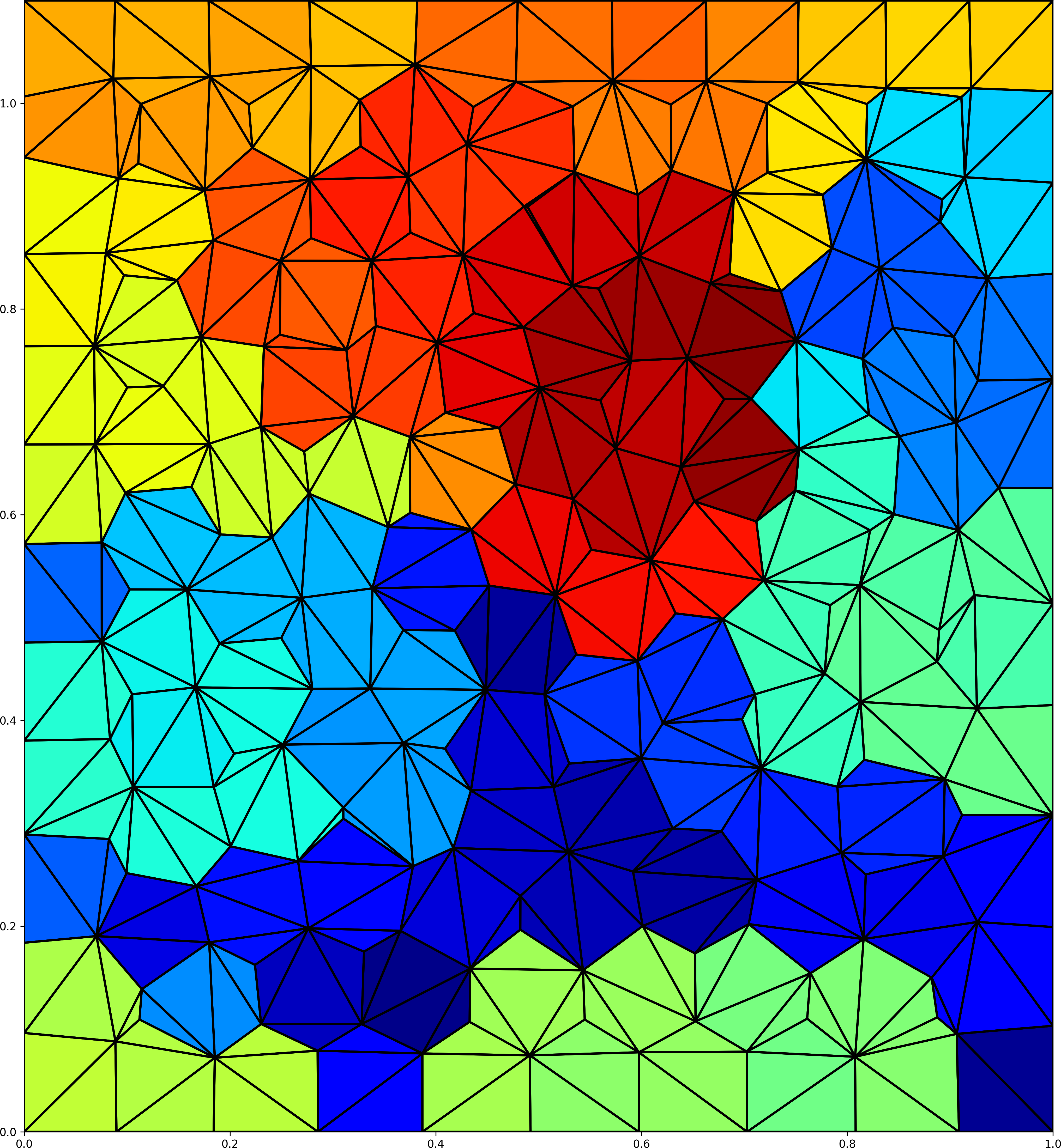
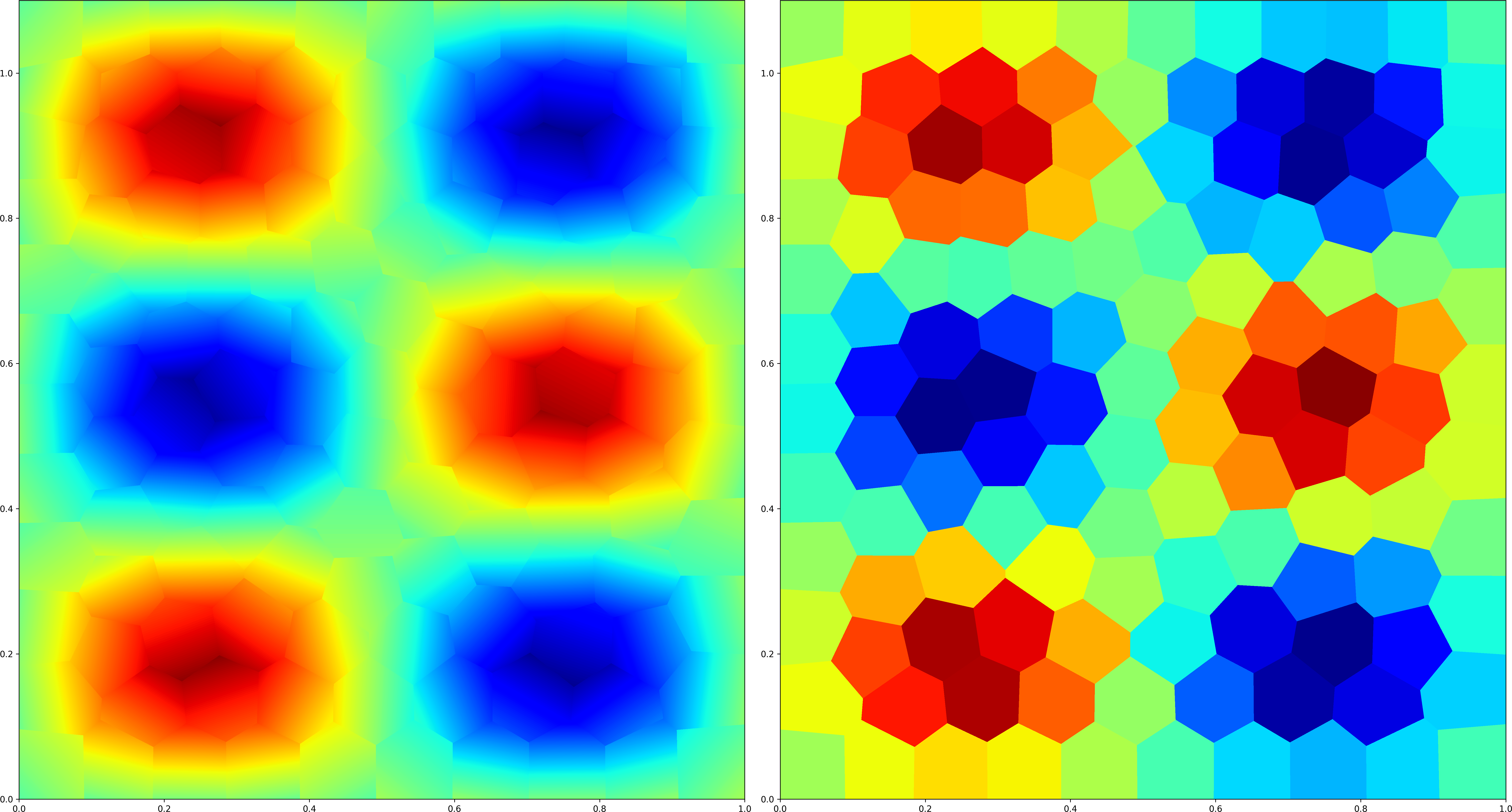
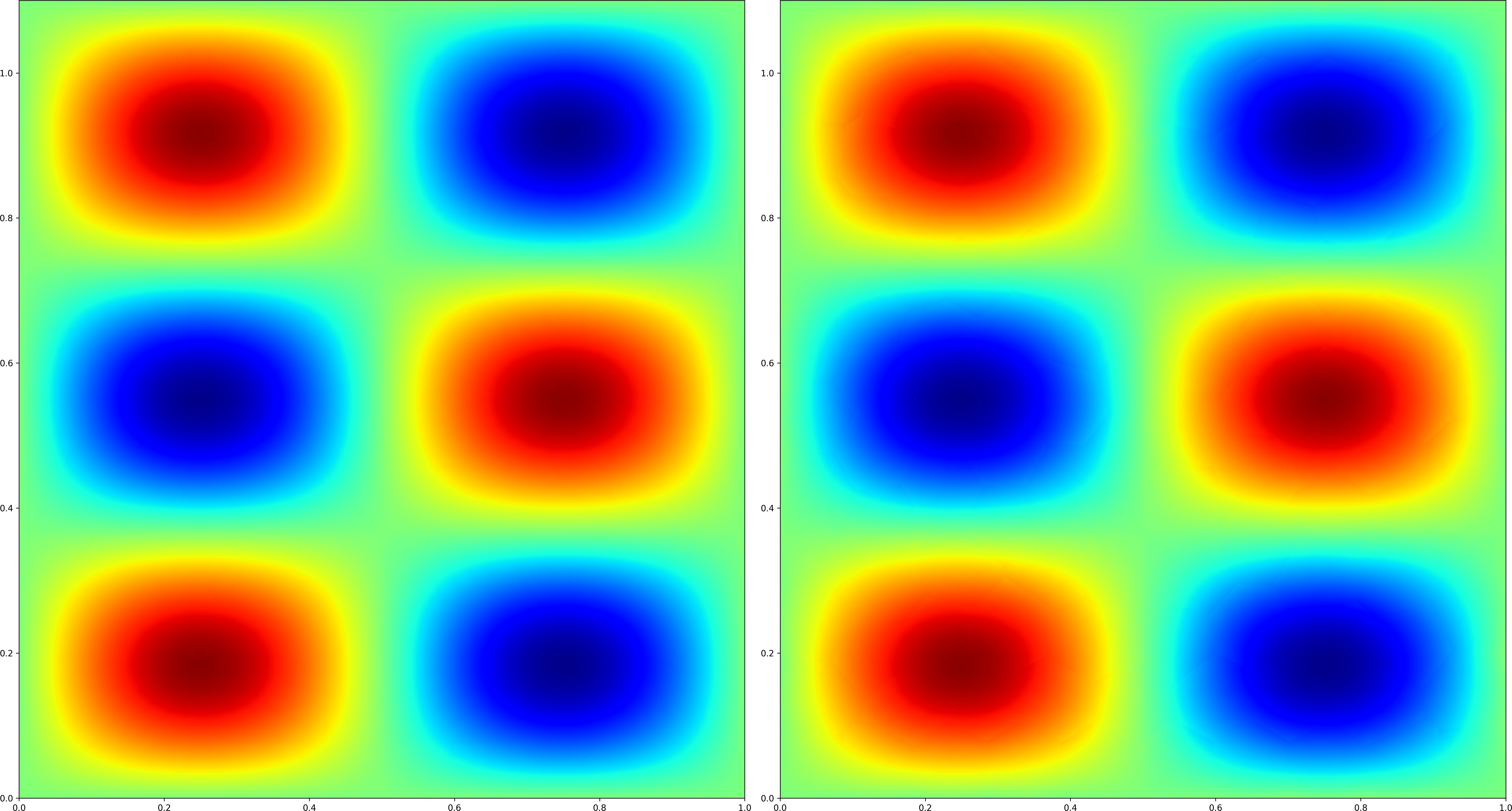
Figure 1: Solutions to the Laplace problem using two different orders for the approximation (left to right) using a Voronoi grid. The left figure shows the grid together with the sub-triangulation used for our agglomeration approach. The next two figures show the solution using a conforming space of order $1$ and the mixed approach with a DG and curl free space of order $0$, respectively. The right two figures show again the primal and mixed solutions but with $\ell=2$ and $\ell=1$, respectively.

7.2 Non-stabilised methods

In this next example we solve both a linear second-order and fourth-order problem using the conforming spaces (Section 3.4.1 and Section 4.2, respectively): find $u\in H^{p}_{0}$ such that

$$a(u,v):=(\kappa(\boldsymbol{x})\nabla^{p}u,\nabla^{p}v)=(f,v)\quad\forall v\in H^{p}_{0},$$

with $p=1$ or $p=2$ and $\kappa(\boldsymbol{x})=\frac{10}{0.01+\boldsymbol{x}\cdot\boldsymbol{x}}$. We set the forcing $f$ so that the exact solution is given by $u(x,y)=(\sin(2\pi x)\sin(2\pi y))^{2}$ on the domain $\Omega=[0,1]^{2}$, and we use a Cartesian grid in both cases.

We test three different variants of the discretisation: (a) the standard version of the spaces with the dofi-dofi stabilisation [11], (b) the standard version of the spaces without any stabilisation, and finally (c) a version of the spaces where the gradient and hessian projections are computed into $[\mathcal{M}_{\ell}(E)]^{2}$ and $[\mathcal{M}_{\ell-1}(E)]^{2\times 2}$ (instead of $\ell-1$ and $\ell-2$ as in the standard case). At the time of writing there is no proof that this will lead to a stable scheme but results shown in Fig. 2 indicate that the non-stabilised method with the extended range spaces for the projections is comparable to the original approach outperforming the non-stabilised method used with the original space which leads to a suboptimal convergence rate.

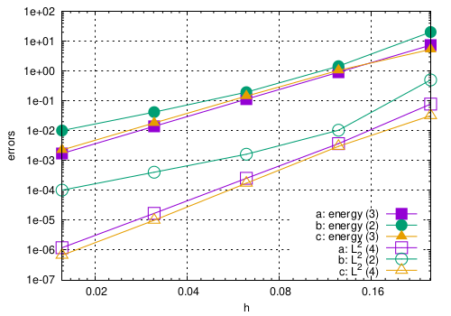
Figure 2: Energy and $L^{2}$-norm errors for different grid resolutions using the stabilised and non-stabilised versions of the VEM discretisation. Left figure shows results for a second-order problem with the $H^{1}$-conforming VEM with order $\ell=3$ and the right figure shows results for a fourth-order problem with the $H^{2}$-conforming VEM with order $\ell=4$. Recall that (a) is the original space with stabilisation, (b) the same space without, and (c) is without stabilisation but with the extended range spaces for the gradient and hessian projections.

7.3 Incompressible flow around a cylinder

We use the divergence free space to solve the Navier-Stokes equations for an incompressible flow with $\nu=0.001$: we seek $(u(t),p(t))$ such that:

$$\partial_{t}u+u\cdot\nabla u-\nu\Delta u+\nabla p =0~{},\quad{\rm div}u=0\quad\text{in }\Omega.$$

Here, $p$ is the pressure and for the velocity $u$ we prescribe the usual initial and boundary conditions for a flow around a cylinder with radius $0.05$ located at $(0.2,0.2)$ in the domain $[0,2.2]\times[0,0.41]$ see e.g. [32, 39]. To discretise this system we use the divergence free space for the velocity and a piecewise constant approximation for the pressure, which is the compatible space containing the divergence of the discrete velocity space. We use a simple discretisation in time based on a semi-implicit method

$$\frac{1}{\tau}u^{n+1}-\nu\Delta u^{n+1}+\nabla p^{n+1} =\frac{1}{\tau}u^{n}-u^{n}\cdot\nabla u^{n}~{},\quad{\rm div}u^{n+1}=0$$

with a time step $\tau=6.25e-4$. The resulting saddle point problem is solved using an Uzawa-type algorithm in each time step. We solve on a triangular grid using different polynomial degrees and compare with results using a more standard Taylor-Hood space. Results are shown in Fig. 3.

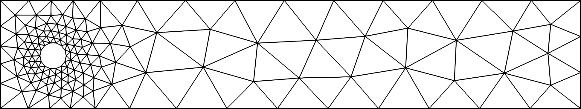
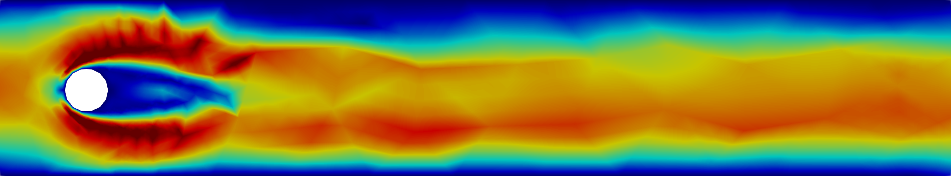
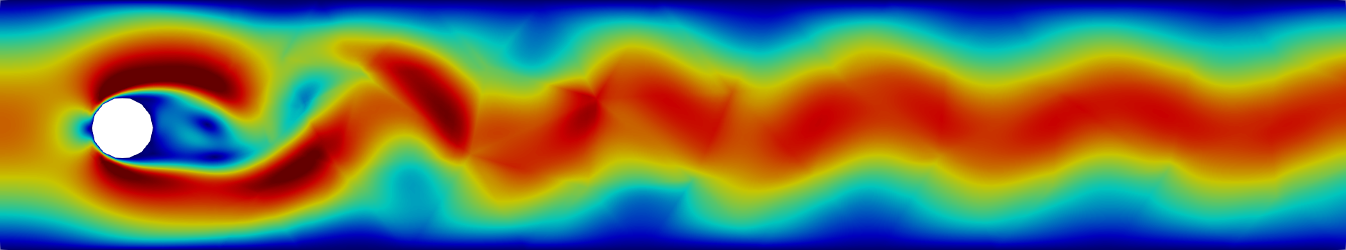
Figure 3: Flow around a cylinder showing magnitude of velocity. On the top left we show the results from using a second-order space for the velocity and piecewise constant pressure on a coarse grid with 260 triangles which itself is shown on the top right figure. On the middle right figure we show the the results from using a fourth-order velocity space and piecewise constant pressure on the same coarse grid. The middle left figure shows results with the same space as top left but on a grid with 1410 triangles having the same resolution around the cylinder but a higher resolution downstream. Bottom left figure shows results using a second-order Taylor Hood space on the same coarse grid shown in the top right figure and finally, the bottom right figure shows results using a fourth-order Taylor Hood space on the same coarse grid.

7.4 Willmore flow of graphs

In our final example we study the minimisation of the Willmore energy of a surface, in the case where the surface is given by a graph over a flat domain $\Omega$. The corresponding Euler-Lagrange equations can be rewritten as a fourth-order problem for a function $u$ defined over $\Omega$. We use a second-order two stage implicit Runge-Kutta method as suggested in [24]. The resulting problem is a system of two nonlinear fourth-order partial differential equations for the two Runge-Kutta stages.

As detailed for example in [24], the Willmore functional for the graph of a function ${u\in W^{2,\infty}(\Omega)}$ is given by

$$W(u)=\frac{1}{2}\int_{\Omega}[\ E(\nabla u):\nabla^{2}u\ ]^{2}\,\mathrm{d}x~{},\;\text{with}\;E_{ij}(w):=\frac{1}{(1+|w|^{2})^{\frac{1}{4}}}\big{(}\delta_{ij}-\frac{w_{i}w_{j}}{1+|w|^{2}}\big{)}$$

for $i,j=1,2$, and $w\in\mathbb{R}^{2}$. We initialise the gradient descent algorithm with $u(x,y)=\big{(}\sin(2\pi x)\sin(2\pi y)\big{)}^{2}$ and we use the time step $\tau=5e-6$ with the $H^{2}$-conforming space from Section 4.2. Fig. 4 shows the evolution of the graph on a Voronoi grid with $800$ cells.

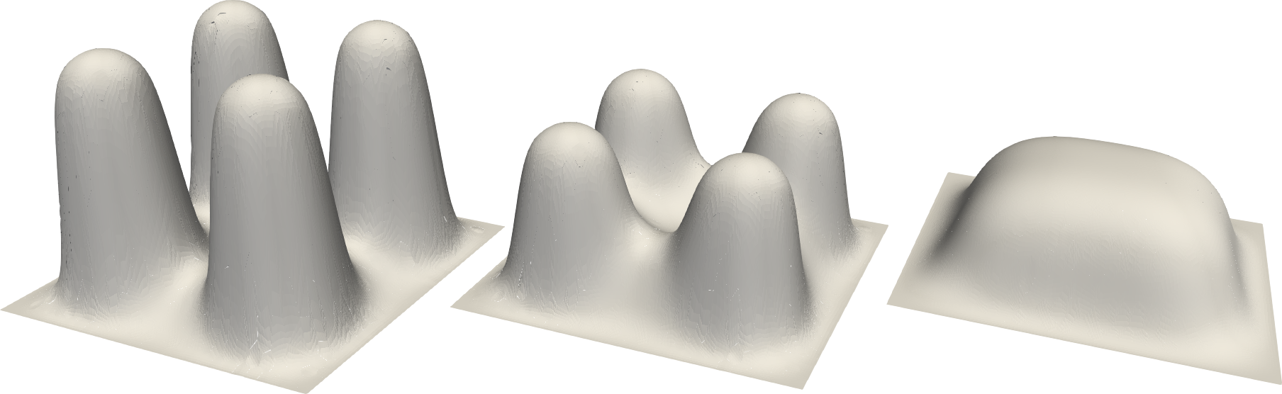
Figure 4: Evolution of a graph under Willmore flow at times $t=1e-4,4e-4,7e-4$ (from left to right) using the $H^{2}$-conforming space of order $\ell=4$. Results with the nonconforming space (also considered in [26]) of the same order are indistinguishable.

8 Conclusion

In this paper, we have presented a framework for implementing general virtual element spaces in two space dimensions and discussed what we believe is a straightforward extension of the framework concepts to three dimensions. As is usual with VEM schemes, the definition of projection operators is crucial in order to setup the discrete bilinear forms. In our approach the definition of the gradient and hessian projections are independent of the space and are based on value projections on the elements and skeleton of the grid. We introduced a VEM tuple for encapsulating all the necessary building blocks for computing these projection operators, a concept which aimed to mimic the FEM triple from the finite element setting. These building blocks included basis sets, dof sets, and constraint sets needed to construct the value projection operators on the elements and skeleton. Additionally, basis sets can be provided for the gradient and hessian projection. Our starting point for the construction of the value projections is constrained least squares problems. Projections for the higher order derivatives are then defined independently of the space. With examples we showed how to construct different VEM spaces with additional properties such as $H^{k}$-conforming spaces for $k=1,2$, divergence free as well as curl free spaces. Our approach has the added benefit of encapsulating extra properties of the space through the value projection. This avoids requiring further projection operators for e.g. the divergence, thus simplifying integration into existing frameworks.

One major advantage of our framework is that it can be easily integrated into an existing finite element package. As already mentioned the main advantage of the presented formulation is that no special projections depending on the underlying PDE are utilised thus minimising the changes required to existing software frameworks. We demonstrated this in two space dimensions within the Dune software framework and presented a handful of numerical experiments to showcase the wide variety of VEM spaces which can be utilised. To the best of our knowledge, this is the first available implementation to include such a vast collection of VEM spaces including but not limited to, spaces for fourth-order problems and nonlinear problems. The software is free and open source and the dune-vem module can be easily installed using PyPI.

References

- [1] B. Ahmad, A. Alsaedi, F. Brezzi, L. D. Marini, and A. Russo, Equivalent projectors for virtual element methods, Comput. Math. Appl., 66 (2013), pp. 376–391, https://doi.org/10.1016/j.camwa.2013.05.015.
- [2] M. Alnæs, J. Blechta, J. Hake, A. Johansson, B. Kehlet, A. Logg, C. Richardson, J. Ring, M. E. Rognes, and G. N. Wells, The FEniCS project version 1.5, Archive of Numerical Software, 3 (2015), https://doi.org/10.11588/ans.2015.100.20553.
- [3] M. S. Alnæs, A. Logg, K. B. Ølgaard, M. E. Rognes, and G. N. Wells, Unified form language: A domain-specific language for weak formulations of partial differential equations, ACM Trans. Math. Softw., 40 (2014), https://doi.org/10.1145/2566630.
- [4] P. F. Antonietti, L. Beirão da Veiga, and G. Manzini, The virtual element method and its applications, vol. 31 of SEMA SIMAI, Springer, Berlin, Heidelberg, 2022, https://doi.org/10.1007/978-3-030-95319-5.
- [5] P. F. Antonietti, L. Beirão da Veiga, S. Scacchi, and M. Verani, A virtual element method for the Cahn–Hilliard equation with polygonal meshes, SIAM J. Numer. Anal., 54 (2016), pp. 34–56, https://doi.org/10.1137/15M1008117.
- [6] P. F. Antonietti, G. Manzini, and M. Verani, The fully nonconforming virtual element method for biharmonic problems, Math. Models Methods Appl. Sci., 28 (2018), pp. 387–407, https://doi.org/10.1142/S0218202518500100.
- [7] P. F. Antonietti, G. Manzini, and M. Verani, The conforming virtual element method for polyharmonic problems, Comput. Math. Appl., 79 (2020), pp. 2021–2034, https://doi.org/10.1016/j.camwa.2019.09.022.
- [8] B. Ayuso de Dios, K. Lipnikov, and G. Manzini, The nonconforming virtual element method, ESAIM Math. Model. Numer. Anal., 50 (2016), pp. 879–904, https://doi.org/10.1051/m2an/2015090.
- [9] W. Bangerth, R. Hartmann, and G. Kanschat, deal.II—A general purpose object-oriented finite element library, ACM Trans. Math. Softw., 33 (2007), pp. 24–es, https://doi.org/10.1145/1268776.1268779.
- [10] P. Bastian, M. Blatt, A. Dedner, C. Engwer, R. Klöfkorn, R. Kornhuber, M. Ohlberger, and O. Sander, A generic grid interface for parallel and adaptive scientific computing. part II: Implementation and tests in DUNE, Computing, 82 (2008), pp. 121–138, https://doi.org/10.1007/s00607-008-0004-9.
- [11] L. Beirão da Veiga, F. Brezzi, A. Cangiani, G. Manzini, L. D. Marini, and A. Russo, Basic principles of virtual element methods, Math. Models Methods Appl. Sci., 23 (2013), pp. 199–214, https://doi.org/10.1142/S0218202512500492.
- [12] L. Beirão Da Veiga, F. Brezzi, L. Marini, and A. Russo, Serendipity nodal VEM spaces, Comput. & Fluids, 141 (2016), pp. 2–12, https://doi.org/10.1016/j.compfluid.2016.02.015.
- [13] L. Beirão da Veiga, F. Brezzi, L. D. Marini, and A. Russo, Virtual element method for general second-order elliptic problems on polygonal meshes, Math. Models Methods Appl. Sci., 26 (2016), pp. 729–750, https://doi.org/10.1142/S0218202516500160.
- [14] L. Beirão da Veiga, C. Lovadina, and G. Vacca, Divergence free virtual elements for the Stokes problem on polygonal meshes, ESAIM Math. Model. Numer. Anal., 51 (2015), pp. 509–535, https://doi.org/10.1051/m2an/2016032.
- [15] L. Beirão da Veiga and G. Manzini, A virtual element method with arbitrary regularity, IMA J. Numer. Anal., 34 (2014), pp. 759–781, https://doi.org/10.1093/imanum/drt018.
- [16] L. Beirão da Veiga, D. Mora, G. Rivera, and R. Rodríguez, A virtual element method for the acoustic vibration problem, Numer. Math., 136 (2017), pp. 725–763, https://doi.org/10.1007/s00211-016-0855-5.
- [17] S. Berrone, A. Borio, and F. Marcon, Lowest order stabilization free virtual element method for the Poisson equation, arXiv preprint arXiv:2103.16896, (2021), https://arxiv.org/abs/2103.16896.
- [18] Å. Björck, Numerical methods for least squares problems, SIAM, 1996.
- [19] F. Brezzi and L. D. Marini, Virtual element methods for plate bending problems, Comput. Methods Appl. Mech. Engrg., 253 (2013), pp. 455–462, https://doi.org/10.1016/j.cma.2012.09.012.
- [20] A. Cangiani, G. Manzini, and O. J. Sutton, Conforming and nonconforming virtual element methods for elliptic problems, IMA J. Numer. Anal., 37 (2017), pp. 1317–1354, https://doi.org/10.1093/imanum/drw036.
- [21] L. Chen and X. Huang, Nonconforming virtual element method for -th order partial differential equations in , Math. Comp., 89 (2020), pp. 1711–1744, https://doi.org/10.1090/mcom/3498.
- [22] P. G. Ciarlet, The finite element method for elliptic problems, North-Holland Publishing Company, 1987.
- [23] F. Dassi and G. Vacca, Bricks for the mixed high-order virtual element method: projectors and differential operators, Appl. Numer. Math., 155 (2020), pp. 140–159, https://doi.org/10.1016/j.apnum.2019.03.014.
- [24] K. Deckelnick, J. Katz, and F. Schieweck, A –finite element method for the Willmore flow of two-dimensional graphs, Math. Comp., 84 (2015), pp. 2617–2643, https://doi.org/10.1090/mcom/2973.
- [25] A. Dedner and A. Hodson, A higher order nonconforming virtual element method for the Cahn-Hilliard equation, arXiv preprint arXiv:2111.11408, (2021), https://arxiv.org/abs/2111.11408.
- [26] A. Dedner and A. Hodson, Robust nonconforming virtual element methods for general fourth-order problems with varying coefficients, IMA J. Numer. Anal., 42 (2022), pp. 1364–1399, https://doi.org/10.1093/imanum/drab003.
- [27] A. Dedner, R. Kloefkorn, and M. Nolte, Python bindings for the DUNE-FEM module, Zenodo, (2020), https://doi.org/10.5281/zenodo.3706994.
- [28] A. Dedner, R. Klöfkorn, M. Nolte, and M. Ohlberger, A generic interface for parallel and adaptive discretization schemes: abstraction principles and the DUNE-FEM module, Computing, 90 (2010), pp. 165–196, https://doi.org/10.1007/s00607-010-0110-3.
- [29] A. Dedner and M. Nolte, Construction of local finite element spaces using the generic reference elements, in Advances in DUNE, A. Dedner, B. Flemisch, and R. Klöfkorn, eds., Berlin, Heidelberg, 2012, Springer Berlin Heidelberg, pp. 3–16.
- [30] F. Hecht, New development in FreeFem++, J. Numer. Math., 20 (2012), pp. 251–266, https://doi.org/10.1515/jnum-2012-0013.
- [31] C. Herrera, R. Corrales-Barquero, J. Arroyo-Esquivel, and J. G. Calvo, A numerical implementation for the high-order 2D virtual element method in MATLAB, Numer. Algorithms, (2022), pp. 1–15, https://doi.org/10.1007/s11075-022-01361-4.
- [32] V. John, Higher order finite element methods and multigrid solvers in a benchmark problem for the 3D Navier–Stokes equations, Internat. J. Numer. Methods Fluids, 40 (2002), pp. 775–798, https://doi.org/10.1002/fld.377.
- [33] B. Kalyanaraman and S. Kehsav, iVEM: a Matlab implementation of the virtual element method, (2021), https://doi.org/10.5281/zenodo.4561721.
- [34] L. Mascotto, Ill-conditioning in the virtual element method: Stabilizations and bases, Numer. Methods Partial Differential Equations, 34 (2018), pp. 1258–1281, https://doi.org/10.1002/num.22257.
- [35] L. S. D. Morley, The triangular equilibrium element in the solution of plate bending problems, Aeronautical Quarterly, 19 (1968), pp. 149–169, https://doi.org/10.1017/S0001925900004546.
- [36] A. Ortiz-Bernardin, C. Alvarez, N. Hitschfeld-Kahler, A. Russo, R. Silva-Valenzuela, and E. Olate-Sanzana, Veamy: an extensible object-oriented C++ library for the virtual element method, Numer. Algorithms, 82 (2019), pp. 1189–1220, https://doi.org/10.1007/s11075-018-00651-0.
- [37] C. Prud’Homme, V. Chabannes, V. Doyeux, M. Ismail, A. Samake, and G. Pena, Feel++ : A computational framework for Galerkin Methods and Advanced Numerical Methods, in ESAIM Proc., vol. 38, EDP Sciences, 2012, pp. 429–455, https://doi.org/10.1051/proc/201238024.
- [38] F. Rathgeber, D. A. Ham, L. Mitchell, M. Lange, F. Luporini, A. T. McRae, G.-T. Bercea, G. R. Markall, and P. H. Kelly, Firedrake: automating the finite element method by composing abstractions, ACM Trans. Math. Softw., 43 (2016), pp. 1–27, https://doi.org/10.1145/2998441.
- [39] M. Schäfer, S. Turek, F. Durst, E. Krause, and R. Rannacher, Benchmark computations of laminar flow around a cylinder, in Flow simulation with high-performance computers II, Springer, 1996, pp. 547–566.
- [40] O. J. Sutton, The virtual element method in 50 lines of MATLAB, Numer. Algorithms, 75 (2017), pp. 1141–1159, https://doi.org/10.1007/s11075-016-0235-3.
- [41] J. Zhao, B. Zhang, S. Chen, and S. Mao, The Morley-type virtual element for plate bending problems, J. Sci. Comput., 76 (2018), pp. 610–629, https://doi.org/10.1007/s10915-017-0632-3.