Thread/State correspondence: the qubit threads model of holographic gravity

Abstract

We construct a new toy model of the holographic principle, named as holographic qubit threads model, which is an enlightening step towards the issue of spacetime emergence (“it from qubit”). More specifically, we propose for the first time that each bit thread in a locking bit thread configuration is in a “qubit” state, i.e., the quantum superposition state of two orthogonal states. Using this thread/state correspondence, we can construct the explicit expressions for the SS states corresponding to a set of bulk extremal surfaces in the surface/state correspondence, and nicely characterize their entanglement structure. Then we use the locking bit thread configurations to construct the holographic qubit threads model, and we show that it is closely related to the holographic tensor networks, kinematic space, and the connectivity of spacetime.

I Introduction

How to unify or reconcile quantum mechanics and general relativity is undoubtedly the most important problem in physics. Advances in recent decades suggest that we may have found an important and marvelous clue to the mystery between gravity and quantum mechanics. This clue is successively related to the concepts of the black hole area entropy Bekenstein:1972tm ; Bekenstein:1973ur ; Bekenstein:1974ax ; Bardeen:1973gs , the holographic principle (especially AdS/CFT duality) Maldacena:1997re ; Gubser:1998bc ; Witten:1998qj , and the RT formula of the holographic entanglement entropy Ryu:2006bv ; Ryu:2006ef ; Hubeny:2007xt , which have built a bridge between quantum mechanics and general relativity. In particular, the RT formula shows that the entanglement entropy that characterizes quantum entanglement between different parts of a particular class of (i.e., “holographic”) quantum systems can be equivalently (i.e., “dually”) described by the area of an extremal surface in a corresponding curved spacetime Ryu:2006bv ; Ryu:2006ef ; Hubeny:2007xt .

More recently, many enlightening ideas from other fields, such as condensed matter physics, quantum information theory, network flow optimization theory, etc., have entered and benefited the study of the holographic gravity. One of the most striking examples is that inspired by the tensor network method originally used in condensed matter physics as a numerical simulation tool to investigate the wave functions of quantum many-body systems, various holographic tensor network (TN) models have been constructed as toy models of the holographic duality Vidal:2007hda ; Vidal:2008zz ; Swingle:2009bg ; Swingle:2012wq ; Pastawski:2015qua ; Hayden:2016cfa ; Chen:2021ipv ; Bao:2018pvs ; Bao:2019fpq ; Lin:2020ufd ; SinaiKunkolienkar:2016lgg ; Qi:2013caa ; Sun:2019ycv ; Haegeman:2011uy . Furthermore, inspired by the continuous version of the holographic tensor network models, Miyaji:2015fia ; Miyaji:2015yva proposed the so-called SS correspondence (surface/state correspondence) as a more specific mechanism of the holographic principle. The SS duality refers to the duality between a codimension two convex surface $\Sigma$ in the holographic bulk spacetime and a quantum state described by a density matrix $\rho(\Sigma)$, which is defined on the Hilbert space of the quantum theory dual to the Einstein’s gravity.

Another idea to further explore the profound connection between spacetime geometry and quantum entanglement is inspired by the optimization problem in network flow theory. Freedman:2016zud ; Cui:2018dyq ; Headrick:2017ucz developed the optimization theory of flows on manifolds, endowed with the name of “bit threads”, and proposed the concept of bit threads can equivalently formulate the RT formula. In this letter, by studying the connection between bit threads and SS duality, we propose a natural and novel physical property of bit threads, dubbed “thread/state correspondence”, that is, in a so-called locking bit thread configuration Headrick:2020gyq ; Lin:2020yzf ; Lin:2021hqs ; Lin:2022aqf , each bit thread is in a quantum superposition state of two orthogonal states. Since the flux of bit threads is directly related to the geometry of a holographic spacetime, while this thread-state property can cleverly characterize quantum entanglement as one will see, it can be expected to be a very useful advance in the study of the relationship between quantum entanglement and spacetime geometry. Note that because bit threads are visually intuitive, they have usually been interpreted implicitly as the bell pairs distilled from the boundary quantum systems, however, they are mostly used merely as a mathematical tool to study different aspects of the holographic principle (see e.g. Lin:2022aqf ; Lin:2021hqs ; Lin:2020yzf ; Headrick:2020gyq ; Agon:2021tia ; Rolph:2021hgz ; Hubeny:2018bri ; Agon:2018lwq ; Du:2019emy ; Harper:2019lff ; Agon:2019qgh ; Agon:2020mvu ; Pedraza:2021fgp ; Pedraza:2021mkh ; Harper:2018sdd ; Shaghoulian:2022fop ; Susskind:2021esx ; Kudler-Flam:2019oru ; Headrick:2022nbe ; Harper:2021uuq ; Harper:2022sky ). Our thread/state rules explicitly accentuate for the first time the implied meaning of the name “bit threads”, namely, that these threads, which are used mathematically to recover the RT formula, can be physically assigned a meaning closely related to the concept of “bits”.

Using thread/state rules, we can do (but expect to do more than) the following things: we can construct the explicit expressions for the SS states corresponding to a set of bulk extremal surfaces in the SS duality, and nicely characterizing their entanglement structure; use the locking bit thread configurations to construct a new toy model of the holographic principle and actually, we explicitly give the relationship between this model and the holographic tensor network models; naturally understand the so-called kinematic space Czech:2015kbp ; Czech:2015qta , endow it with the interpretation of microscopic states such that to explain that the entropy is proportional to volume therein; in some sense quantitatively characterize the famous “It from qubit” thought experiment VanRaamsdonk:2010pw , that is, by removing the entanglement in the boundary quantum system, the bulk spacetime will accordingly deform, or even break up.

The idea of thread state will provide a complementary perspective distinct from the local tensors used in holographic TN models. Moreover, our thread/state prescription for locking thread configurations is an enlightening step towards the issue of spacetime emergence. It is intriguing to find the similar rules for the more general non-locking bit thread configurations, then it is possible to further read the SS states of the general bulk surfaces. It is even more tantalizing to completely reconstruct the bulk geometry merely from the properties of the quantum state assigned to the bit threads. In addition, it is also interesting to consider how the thread/state rules adapt to the covariant bit threads Headrick:2022nbe of the covariant RT formula Hubeny:2007xt , the quantum bit threads Agon:2021tia ; Rolph:2021hgz that can account for the bulk quantum corrections to the RT formula Faulkner:2013ana ; Engelhardt:2014gca , the Lorentzian bit threads Pedraza:2021fgp ; Pedraza:2021mkh that can characterize the holographic complexity Brown:2015bva ; Susskind:2014rva , the hyperthreads Harper:2021uuq ; Harper:2022sky that can study the multipartite entanglement, and so on, and may provide useful insights on all of these topics.

II Prescription: thread/state correspondence

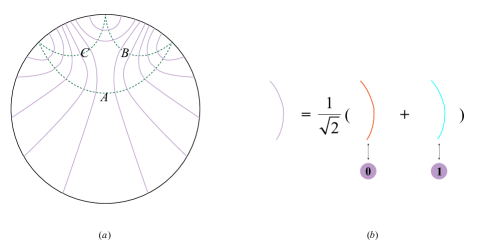
Figure 1: (a) A locking bit thread configuration that locks three RT surfaces $A$, $B$, and $C$ simultaneously. (b) Thread/state correspondence.

The motivation of thread/state correspondence originated from finding an effective scheme to characterize the entanglement structure between different bulk extremal surfaces in the framework of SS duality, or explicitly constructing the dual states (hereinafter referred to as SS states) of these extremal surfaces. This is inspired by the following two notable simple rules in the SS duality Miyaji:2015fia ; Miyaji:2015yva ; Lin:2020ufd : $\bf rule~{}1:$ the density matrix corresponding to an extremal surface is a direct product of the density matrices at each point. In other words, a bulk extremal surface corresponds to an equal-probability mixed state; $\bf rule~{}2:$ a closed surface corresponds to a pure state. Due to rule 1, one can imagine that on an extremal surface associated with an entropy $S$ (i.e., with an area of $4{G_{N}}S$), there distribute exactly $S$ bits (each with only two basic states, $\left|1\right\rangle$ and $\left|0\right\rangle$). Then, for any bulk extremal surface $\gamma$ with an entropy ${S_{\gamma}}$, we can label its basic states as $\left\{{\left|{\gamma=q}\right\rangle\left|{q\in N,0\leq q\leq{2^{{S_{\gamma}}}}-1}\right.}\right\}$. Each decimal number $q$ exactly corresponds to a binary string that describes the overall configuration state of all the SS bits on $\gamma$. The SS state corresponding to $\gamma$ can be represented as a mixed state ${\rho_{\gamma}}$ equipped with equal probabilities Lin:2020ufd :

$${\rho_{\gamma}}=\sum\limits_{q=0}^{{2^{{S_{\gamma}}}}-1}{\frac{1}{{{2^{{S_{\gamma}}}}}}\left|{\gamma=q}\right\rangle\left\langle{\gamma=q}\right|}.$$ (1)

Now we present the thread/state prescription. In the framework of the holographic principle, bit threads are defined as divergenceless but unoriented bulk threads whose density is less than $1/4{G_{N}}$ everywhere Freedman:2016zud ; Cui:2018dyq ; Headrick:2017ucz . Bit threads can be described by the language of $multiflow$. In particular, a bit thread configuration that can simultaneously optimize (i.e., maximize, or “lock”) a set of thread fluxes through some specified boundary regions is referred to as a locking bit thread configuration Headrick:2020gyq . We will show that, following the prescription, a locking bit thread configuration can automatically determine the explicit form of the SS states of the bulk extremal surfaces.

Consider a locking bit thread configuration that can lock three regions $A$, $B$, and $C$ (which are three RT extremal surfaces) simultaneously, as shown in figure 1(a). Denote the numbers of threads connecting $AB$, $AC$, and $BC$ in the configuration as ${F_{AB}}$, ${F_{AC}}$, and ${F_{BC}}$ respectively, which are exactly half of the mutual information ${I_{AB}}$, ${I_{AC}}$, and ${I_{BC}}$ Lin:2020yzf . The thread/state correspondence prescription is as follows:

$(\bf 1)$ Each bit thread has two possible orthogonal states, namely $\left|{{\rm{red}}}\right\rangle$ state and $\left|{{\rm{blue}}}\right\rangle$ state. The same bit thread is always in a same “color” state, or a same superposition state of the color states, while the state of one bit thread does not affect the state of the other bit thread.

$(\bf 2)$ In a locking bit thread configuration, each bit thread is in a special quantum superposition state:

$$\left|{{\rm{thread}}}\right\rangle=\frac{1}{{\sqrt{2}}}\left({\left|{{\rm{red}}}\right\rangle+\left|{{\rm{blue}}}\right\rangle}\right)$$ (2)

$(\bf 3)$ In a locking bit thread configuration, the bit threads exactly meet the SS bits on the intersecting bulk extremal surfaces. The red state of a bit thread corresponds to the $\left|0\right\rangle$ state of the SS bits it passes through on the bulk extremal surfaces, while the blue state corresponds to the $\left|1\right\rangle$ state. In fact, this correspondence can be written more explicitly as

$$\begin{array}[]{l}\left|{{\rm{red}}}\right\rangle=\left|{00\cdots 00}\right\rangle\\ \left|{{\rm{blue}}}\right\rangle=\left|{11\cdots 11}\right\rangle\end{array}$$ (5)

In other words, if we perform a measurement operation to make a bit thread in a certain color state, the SS bits crossed by the same red bit thread will be all in the certain $\left|0\right\rangle$ state, while the SS bits crossed by the same blue bit thread will be all in the certain $\left|1\right\rangle$ state.

Using the thread/state rules, we end up with an explicit form of the state of the whole closed surface $ABC$ as (see Appendix A for details):

$$\begin{array}[]{l}\left|\Psi\right\rangle=\sum\limits_{{q_{AB}}=0}^{{2^{{F_{AB}}}}-1}{\sum\limits_{{q_{AC}}=0}^{{2^{{F_{AC}}}}-1}{\sum\limits_{{q_{BC}}=0}^{{2^{{F_{BC}}}}-1}{\frac{1}{{\sqrt{{2^{{F_{AB}}+{F_{AC}}+{F_{BC}}}}}}}}}}\\ \cdot\left({\left|{{\phi_{AB}}={q_{AB}}}\right\rangle\otimes\left|{{\phi_{AC}}={q_{AC}}}\right\rangle}\right)\\ \otimes\left({\left|{{\phi_{AB}}={q_{AB}}}\right\rangle\otimes\left|{{\phi_{BC}}={q_{BC}}}\right\rangle}\right)\\ \otimes\left({\left|{{\phi_{AC}}={q_{AC}}}\right\rangle\otimes\left|{{\phi_{BC}}={q_{BC}}}\right\rangle}\right)\end{array},$$ (10)

where $\left|{{\phi_{AB}}={q_{AB}}}\right\rangle=\left|{\overbrace{--\cdots--}^{{F_{AB}}}}\right\rangle$ represents a configuration state of the bit threads connecting $A$ and $B$, whose number is ${F_{AB}}$, and it also provides the information of the configuration states of the SS bits on the bulk extremal surfaces that these bit threads pass through. The similar notation is used for ${\phi_{AC}}$ and ${\phi_{BC}}$. Note that (10) is indeed a pure state, and the key point is that it is not difficult to verify that this expression (10) can indeed be reduced to the correct reduced density matrixes (1) of $A$, $B$, and $C$.

A physical comment: because of the quantum entanglement between $B$ and $C$, the Hilbert space dimension of the states of $BC$ as a whole is exactly equal to the Hilbert space dimension of the corresponding states of $A$. Our thread/state correspondence rules explicitly show how the bit threads characterize the quantum entanglement between $B$ and $C$: that is, the SS bits on surfaces $B$ and $C$ crossed by the same bit thread must be in the same state.

Moreover, it is immediately to apply this method to the case involving more RT surfaces. As long as the corresponding locking bit thread configuration is constructed, the SS states of these RT surfaces can be read out at the same time.

III Holographic qubit threads model

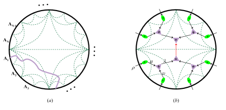
Figure 2: (a) The holographic qubit threads model. We only present one component flow (the thick mauve line) schematically. The green dashed lines represent a set of non-intersecting RT surfaces. (b) Match with a holographic tensor network model.

Inspired by the thread/state correspondence, it is natural to construct a novel toy model of the holographic principle, as shown in figure 2(a). We can divide the holographic boundary quantum system into extremely large $N$ non-overlapping adjacent subregions (called $elementary~{}regions$), denoted as ${A_{1}}$, ${A_{2}}$, …, ${A_{N}}$, then introduce a $multiflow$ composed of $N\left({N-1}\right)/2$ $component~{}flows$ to describe a locking thread configuration that can lock all these elementary regions and a set of non-intersecting $composite~{}regions$ (the unions of elementary regions) simultaneously. In addition, we also require that each component flow flux in the locking bit thread configuration satisfies the so-called “CFF=PEE” scheme Lin:2021hqs , i.e.,

$${F_{ij}}=\frac{1}{2}\left({S\left({\tilde{A}\cup{A_{i}}}\right)+S\left({\tilde{A}\cup{A_{j}}}\right)-S\left({\tilde{A}}\right)-S\left({{A_{i}}\cup\tilde{A}\cup{A_{j}}}\right)}\right),$$ (11)

where we denote the region sandwiched between ${A_{i}}$ and ${A_{j}}$ as $\tilde{A}={A_{\left({i+1}\right)\cdots\left({j-1}\right)}}$ .  This is for each component flow flux (CFF) to exactly match the partial entanglement entropy (PEE) in the boundary quantum system one by one, so as to reflect the entanglement structure information of the boundary quantum system correctly and reasonably. Using the convex dualization technique in the convex optimization theory and the bulk-cell decomposition method proposed in Headrick:2020gyq (see also Lin:2020yzf ), we can prove that a locking thread configuration can lock a specified set of non-intersecting boundary regions simultaneously while subject to the extra constraints (11) at the same time always exists. See app for details.

According to the thread/state prescription, and following the previous notation, then one can write out the explicit density matrix of each RT surface directly. For a general connected boundary composite region $R={A_{a\left({a+1}\right)\cdots b}}\equiv{A_{a}}\cup{A_{a+1}}\cup\cdots\cup{A_{b}}$, the SS state of its corresponding holographic RT surface ${\gamma_{a\left({a+1}\right)\cdots b}}$ can be expressed as follows:

$$\begin{array}[]{l}{\rho_{{\gamma_{a\left({a+1}\right)\cdots b}}}}=\sum\limits_{s,t}{\sum\limits_{{q_{st}}=0}^{{2^{{F_{st}}}}-1}{\frac{1}{{{2^{{S_{a\left({a+1}\right)\cdots b}}}}}}}}\\ \cdot\left({\prod\limits_{s,t}{\left|{{\phi_{st}}={q_{st}}}\right\rangle}}\right)\left({\prod\limits_{s,t}{\left\langle{{\phi_{st}}={q_{st}}}\right|}}\right)\end{array}$$ (14)

where $s\in\left\{{a,a+1,\cdots,b}\right\}$, $t\notin\left\{{a,a+1,\cdots,b}\right\}$.

IV Relation with holographic tensor network mo dels

Our holographic qubit threads model is closely related to the holographic tensor network models (the preliminary discussion on the connection between bit threads and holographic tensor networks can be seen in Lin:2020yzf ). In fact, it is natural to convert the former form into the latter form. The key point is that a part of the whole thread configuration in each bulk “cell” divided by the RT surfaces can be written as a tensor using the thread/state prescription. In particular, these tensors can just be understood as the $disentanglers$ in the holographic tensor networks Vidal:2007hda ; Vidal:2008zz ; Swingle:2009bg ; Swingle:2012wq .

More explicitly, as shown in figure 2(b), one can construct two kinds of tensors using thread/state correspondence, denoted as $V$ and $W$. Wherein $V$ represents the distillation tensor Bao:2018pvs ; Bao:2019fpq ; Lin:2020ufd , which is defined as mapping the reduced state of each boundary elementary region to the SS state associated with its RT surface. In this paper, we do not focus on the study of $V$ tensor, which is merely a pro forma definition at the moment. The $W$ tensor plays the role of a $disentangler$ Vidal:2007hda ; Vidal:2008zz ; Swingle:2009bg ; Swingle:2012wq , which maps the SS states of the two RT surfaces in the previous layer to the SS state of the RT surface in the next layer. Notice in the figure we also assign an arrow direction to each leg to specify the upper and lower indices of a tensor, then we can first write the $W$ tensor as $W_{\mu\nu}^{\lambda}$ pro forma, where $\mu$ and $\nu$ represent the SS states of the two RT surfaces of the previous layer, respectively, while $\lambda$ represents the SS state of the RT surface of the inner layer. Then the thread/state correspondence indicates that $\mu$, $\nu$ and $\lambda$ could be further decomposed into smaller indices, thus one can write a universal expression for the $W$ tensor of any layer immediately. We first write down the corresponding pure state of the closed surface that is the boundary of the cell of each layer. Consider a cell consisting of three RT surfaces ${\gamma_{R}}$, ${\gamma_{S}}$ and ${\gamma_{T}}$ corresponding to three adjacent composite boundary regions $R$, $S$ and $T$, respectively. Let us denote $R=\cup{A_{r}}$, $S=\cup{A_{s}}$, $T=\cup{A_{t}}$, i.e., denote the elementary regions within $R$, $S$ and $T$ as ${A_{r}}$, ${A_{s}}$ and ${A_{t}}$ respectively. Following these notations, we can write:

$$\begin{array}[]{l}\left|{{\Psi_{{\gamma_{R}}\cup{\gamma_{S}}\cup{\gamma_{T}}}}}\right\rangle=\left({\sum\limits_{r,t}{\sum\limits_{{q_{rt}}=0}^{{2^{{F_{rt}}}}-1}{}}}\right)\left({\sum\limits_{s,t}{\sum\limits_{{q_{st}}=0}^{{2^{{F_{st}}}}-1}{}}}\right)\left({\sum\limits_{r,s}{\sum\limits_{{q_{rs}}=0}^{{2^{{F_{rs}}}}-1}{}}}\right)\\ \frac{1}{{\sqrt{{2^{\sum\limits_{r,t}{{F_{rt}}}+\sum\limits_{s,t}{{F_{st}}}+\sum\limits_{r,s}{{F_{rs}}}}}}}}\cdot\left({\prod\limits_{r,t}{\left|{{\phi_{rt}}={q_{rt}}}\right\rangle}}\right)\\ \otimes\left({\prod\limits_{s,t}{\left|{{\phi_{st}}={q_{st}}}\right\rangle}}\right)\otimes\left({\prod\limits_{r,s}{\left|{{\phi_{rs}}={q_{rs}}}\right\rangle}}\right)\end{array},$$ (18)

then we obtain

$$\begin{array}[]{l}W_{{\mu_{R}}{\nu_{S}}}^{{\lambda_{T}}}=W_{\left\{{{\mu_{rt}}}\right\}\left\{{{\mu_{rs}}}\right\}\left\{{{\nu_{rs}}}\right\}\left\{{{\nu_{st}}}\right\}}^{\left\{{{\lambda_{rt}}}\right\}\left\{{{\lambda_{st}}}\right\}}\\ \quad\quad\,=\left\{{\begin{array}[]{*{20}{c}}{\frac{1}{{\sqrt{{2^{\sum\limits_{r,t}{{F_{rt}}}+\sum\limits_{s,t}{{F_{st}}}+\sum\limits_{r,s}{{F_{rs}}}}}}}},\quad{\lambda_{ij}}={\mu_{ij}}={\nu_{ij}}}\\ {0.\quad otherwise}\end{array}}\right.\end{array}.$$ (23)

From the expression of (23), it is clear that the lower index of the $W$ tensor has the $rs$ component representing the entanglement between a pair of elementary regions ${A_{r}}$ and ${A_{s}}$, while the upper index has no $rs$ component. Therefore, the $W$ tensor is exactly playing the role of a $disentangler$ (of course, it also plays the role of the $coarse$-$grainer$ at the same time. A preliminary discussion of this issue can be seen in Lin:2020ufd ; Lin:2020yzf ), because it is such a unitary operation that just converts the state of two entangled blocks in the previous layer into a state of a block without internal entanglement. This process of disentanglement can be intuitively understood as removing the contribution of the inner threads that represent the shorter range entanglement! This process is carried out successively, exactly in line with the idea of MERA-like tensor network, that is, the effect of short-range entanglement is successively removed and only the effect of long-range entanglement is finally focused on Vidal:2007hda ; Vidal:2008zz ; Swingle:2009bg ; Swingle:2012wq .

On the other hand, we can directly write the distillation tensor $V$ pro forma as

$$V_{{\rho_{i}}}^{{\mu_{i}}}=V_{{\rho_{i}}}^{\left\{{{\mu_{ij}}}\right\}},$$ (24)

where $j$ runs from 1 to $N$ (except for $j$ itself), and the lower index ${\rho_{i}}$ represents the reduced state of the elementary region ${A_{i}}$, while ${\mu_{i}}$ represents the SS state of the RT surface ${\gamma_{i}}$ corresponding to ${A_{i}}$. For example, for region ${A_{1}}$,

$$V_{{\rho_{1}}}^{{\mu_{1}}}=V_{{\rho_{1}}}^{{\mu_{12}}{\mu_{13}}\cdots{\mu_{1N}}}.$$ (25)

The $V$ tensors are isometries Bao:2018pvs ; Bao:2019fpq ; Lin:2020ufd .

V Relation with kinematic space

Our holographic qubit threads model also has a close connection to the so-called kinematic space app . Kinematic space is an example of the application of quantum information theory to the holographic duality Czech:2015kbp ; Czech:2015qta . Briefly speaking, it is a dual space wherein each point is one-to-one mapped from a pair of points on the boundary of the original geometry. Czech:2015kbp ; Czech:2015qta proposed that in the framework of the holographic principle, the metric of a kinematic space (i.e., its spatial volume density) is defined by the conditional mutual information (CMI),

$$\mathscr{D}g\equiv{d^{2}}{V_{{\rm{kin}}}}={\rm{CMI}},$$ (26)

where

$${\rm{CMI(}}A,C\left|B\right.{\rm{)}}=S(AB)+S(BC)-S(ABC)-S(B),$$ (27)

and the entanglement entropy can be represented by a volume in kinematic space

$$S\propto{\rm{Vol}}.$$ (28)

Naturally, we can relate each thread in our holographic qubit threads model to a point in a kinematic space. Moreover, seeing (11), CMI and PEE (or our component flow flux, CFF) are exactly the same thing characterizing the entanglement density in a sense. The point is that according to our thread/state correspondence, now every point in kinematic space can be just interpreted as a qubit, namely a quantum superposition of two orthogonal basic states. Therefore, in fact, our thread/state rules can be regarded as indicating the microstates of the kinematic space. By thread/state rules,

$$S\propto\ln\Omega=\ln\left({{2^{\sum{{F_{ij}}}}}}\right)=\sum{{F_{ij}}},$$ (29)

by (11),

$$\sum{{F_{ij}}}=\sum{{\rm{CMI}}},$$ (30)

then by (26), one obtain (28).

In other words, simply counting the number of these microstates $\Omega$ leads to the conclusion that the entanglement entropy is proportional to the volume of kinematic space (a natural interpretation). Kinematic space is also closely related to the interpretation of the MERA tensor network Czech:2015kbp ; Czech:2015qta , therefore, we expect that our thread/state correspondence will deepen the understanding of both.

VI Relation with the connectivity of spacetime

Our holographic qubit threads model can visualize the connection between the entanglement of the boundary quantum system and the connectivity of the holographic bulk spacetime. Consider a thought experiment similar to Raamsdonk’s famous “It from qubit” experiment VanRaamsdonk:2010pw , see figure 3. Consider dividing the whole boundary quantum system $M$ into two halves, denoted as ${M_{+}}$ and ${M_{-}}$, then remove the entanglement between the two halves, but still preserve the entanglement between the internal elementary regions within ${M_{+}}$ and those within ${M_{-}}$. Then this implies that the values of bit thread fluxes characterizing the former vanish, while those characterizing the latter are unchanged. Since these vanishing bit threads are originally passing through a series of RT surfaces and thus contributing to all these RT surfaces, not only does the area of the RT surface separating ${M_{+}}$ and ${M_{-}}$ shrink to zero (and thus the original bulk spacetime $N$ is split into two new disconnected independent spacetimes), but the areas of the RT surfaces inside the two halves of $N$ also decreases. Although we still do not fully figure out how to decode the geometric information of any surface or any region in the bulk from the entanglement information in the boundary CFT states completely, however, the area changes of these RT surfaces can quantitatively characterize how the bulk spacetime shrinks and splits as the quantum entanglement is taken away to some extent. This quantitative calculation can in principle be explicitly implemented by the following formula in the locking bit thread configuration Lin:2021hqs :

$$\begin{array}[]{l}{\rm{Are}}{{\rm{a}}_{a\left({a+1}\right)\ldots b}}=4{G_{N}}\sum\limits_{s,t}{{F_{st}}},\\ s\in\left\{{a,a+1,\cdots,b}\right\},t\notin\left\{{a,a+1,\cdots,b}\right\}\end{array},$$ (33)

where ${\rm{Are}}{{\rm{a}}_{a\left({a+1}\right)\ldots b}}$ represents the area of the RT surface associated with a connected composite region $R={A_{a\left({a+1}\right)\cdots b}}\equiv{A_{a}}\cup{A_{a+1}}\cup\cdots\cup{A_{b}}$. This is very interesting. With this splitting process repeating, finally, a bulk spacetime $N$ will eventually disintegrate into a tremendous number of small bubbles. Conversely, this implies that, one can build a continuous spacetime using quantum entanglement. Figuratively speaking, bit threads, or we now should say, “qubit threads” can play the roles of “sewing” a spacetime. The threads extract the entanglement information from the boundary quantum system, and then build a spacetime just like sewing many small fragments into a sweater!

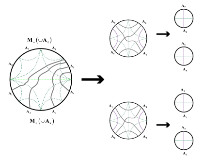
Figure 3: Removing all entanglement between the set of ${A_{s}}$ and the set of ${A_{t}}$ (we only draw a few of relevant thread bundles, i.e., the thick grey lines in the figure), the original bulk spacetime $N$ is split into two independent holographic bulk spacetimes ${N_{+}}$ and ${N_{-}}$. With this process repeating, finally, a bulk spacetime $N$ will eventually disintegrate into a tremendous number of small bubbles.

VII Discussions

The idea of holographic tensor networks or quantum information theory has proved to be enlightening to the issue of spacetime emergence (“it from qubit”), while in this letter we have seen that the concept of (long-range) “threads” can provide a new perspective that is different from, but closely related to the local “tensors” (or quantum circuit gates). Although our thread/state correspondence rules for locking thread configurations merely apply to bulk extremal surfaces at present, it is a suggestive step towards the issue of spacetime emergence. Since the concept of bit threads originates from the duality of the optimization problem of the areas of geometric surfaces and the optimization problem of the fluxes of thread flows, we can further ask whether similar rules can be found and applied to the more general non-locking bit thread configurations so that one can further read the SS states of the more general bulk surfaces. In the longer term, an even more tantalizing idea is to further cast off the metric information of the background spacetime and completely reconstruct the bulk geometry only from the properties of the quantum state assigned to the bit threads.

On the other hand, actually there are various updated versions of bit threads, which are very useful tools for studying various aspects of the relationship between geometry and quantum entanglement, such as the covariant bit threads Headrick:2022nbe , the quantum bit threads Agon:2021tia ; Rolph:2021hgz , the Lorentzian bit threads Pedraza:2021fgp ; Pedraza:2021mkh , the hyperthreads Harper:2021uuq ; Harper:2022sky , etc. It is likely that our thread/state correspondence rules could be further adapt to these similar objects and lead to deeper or clearer understandings of these different important aspects of the holographic duality.

Appendix A A user guide to thread/state prescription

Considering the simplest case involving three RT surfaces ($A$, $B$, and $C$) as shown in figure 1(a), focusing on the correct equal-probability mixed states ${\rho_{A}}$, the pure state corresponding to the whole closed surface $ABC$ can be constructed as

$$\left|\Psi\right\rangle=\sum\limits_{q=0}^{{2^{{S_{A}}}}-1}{\frac{1}{{\sqrt{{2^{{S_{A}}}}}}}\left|{A=q}\right\rangle\otimes\left|{BC=q}\right\rangle},$$ (34)

where $\left|{BC=q}\right\rangle$ is merely a pro forma definition at present, representing the basic states of the complement of region $A$ in the whole closed system. With a little thought, we realize that each of these $\left|{BC=q}\right\rangle$ states should actually be a quantum superposition state of $\left|{\underbrace{--\cdots--}_{{S_{B}}}\underbrace{--\cdots--}_{{S_{C}}}}\right\rangle=\left|{\underbrace{--\cdots--}_{{S_{B}}}}\right\rangle\otimes\left|{\underbrace{--\cdots--}_{{S_{C}}}}\right\rangle\equiv\left|{B={q_{b}}}\right\rangle\otimes\left|{C={q_{c}}}\right\rangle$.

Now suppose we are going to measure surface $A$ and find that $A$ is in a certain configuration after the measurement operation, for example, in the state $\left|{A=0}\right\rangle\equiv\left|{\underbrace{00\cdots 00}_{{S_{A}}}}\right\rangle$. Then by rule 3, this is also equivalent to measuring that all bit threads passing through surface $A$ (i.e., starting from $A$, and connecting to $B$ or $C$) are in red state. As per rule 1, the operation of measuring $A$ will not affect the state of other bit threads that do not cross $A$ (i.e. threads connecting $B$ with $C$), then we can immediately construct the explicit form of the corresponding configuration$\left|{BC=0}\right\rangle$ that $BC$ must be in when $A$ is measured to be in configuration $\left|{A=0}\right\rangle\equiv\left|{\underbrace{00\cdots 00}_{{S_{A}}}}\right\rangle$. Firstly, under this measurement, that $A$ is in configuration $\left|{A=0}\right\rangle\equiv\left|{\underbrace{00\cdots 00}_{{S_{A}}}}\right\rangle$ corresponds to the bit threads passing through surface $A$ (to $B$ or $C$) are all in red state, therefore, in fact, we have determined the states that a certain part of the SS bits on surface $B$ and $C$ must be in, that is, the SS bits passed through by these red bit threads are all in the definite state $\left|0\right\rangle$. On the other hand, the other bits on $B$ and $C$ are passed through by the bit threads in the superposition state (2) (rule 2). Therefore, the prescription automatically produces the specific form of $\left|{BC=0}\right\rangle$ as

$$\begin{array}[]{l}\left|{BC=0}\right\rangle=\chi\cdot\{\left|{\underbrace{\overbrace{00\cdots 00}^{{F_{AB}}}\overbrace{00\cdots 00}^{{F_{BC}}}}_{{S_{B}}}\underbrace{\overbrace{00\cdots 00}^{{F_{AC}}}\overbrace{00\cdots 00}^{{F_{BC}}}}_{{S_{C}}}}\right\rangle\\ +\left|{\underbrace{\overbrace{00\cdots 00}^{{F_{AB}}}\overbrace{00\cdots 01}^{{F_{BC}}}}_{{S_{B}}}\underbrace{\overbrace{00\cdots 00}^{{F_{AC}}}\overbrace{00\cdots 01}^{{F_{BC}}}}_{{S_{C}}}}\right\rangle\\ +\cdots+\left|{\underbrace{\overbrace{00\cdots 00}^{{F_{AB}}}\overbrace{11\cdots 11}^{{F_{BC}}}}_{{S_{B}}}\underbrace{\overbrace{00\cdots 00}^{{F_{AC}}}\overbrace{11\cdots 11}^{{F_{BC}}}}_{{S_{C}}}}\right\rangle\}\end{array},$$ (38)

where $\chi$ is a normalization constant that should satisfy

$${\chi^{2}}\cdot{2^{{F_{BC}}}}=1,$$ (39)

that is,

$$\chi=\frac{1}{{\sqrt{{2^{{F_{BC}}}}}}}=\frac{1}{{\sqrt{{2^{\frac{{{S_{B}}+{S_{C}}-{S_{A}}}}{2}}}}}}.$$ (40)

Similarly, we can use the same reasoning to obtain the explicit form of the corresponding $\left|{BC=q}\right\rangle$ state for each $\left|{A=q}\right\rangle$ state, and finally obtain the expression of the full pure state of the whole system $ABC$ as follows:

$$\begin{array}[]{l}\left|\Psi\right\rangle=\\ \frac{1}{{\sqrt{{2^{{F_{AB}}+{F_{AC}}}}}}}\left|{\underbrace{\overbrace{00\cdots 00}^{{F_{AB}}}\overbrace{00\cdots 00}^{{F_{AC}}}}_{{S_{A}}}}\right\rangle\otimes\{\frac{1}{{\sqrt{{2^{{F_{BC}}}}}}}(\left|{\underbrace{\overbrace{00\cdots 00}^{{F_{AB}}}\overbrace{00\cdots 00}^{{F_{BC}}}}_{{S_{B}}}\underbrace{\overbrace{00\cdots 00}^{{F_{AC}}}\overbrace{00\cdots 00}^{{F_{BC}}}}_{{S_{C}}}}\right\rangle\\ +\left|{\underbrace{\overbrace{00\cdots 00}^{{F_{AB}}}\overbrace{00\cdots 01}^{{F_{BC}}}}_{{S_{B}}}\underbrace{\overbrace{00\cdots 00}^{{F_{AC}}}\overbrace{00\cdots 01}^{{F_{BC}}}}_{{S_{C}}}}\right\rangle+\cdots+\left|{\underbrace{\overbrace{00\cdots 00}^{{F_{AB}}}\overbrace{11\cdots 11}^{{F_{BC}}}}_{{S_{B}}}\underbrace{\overbrace{00\cdots 00}^{{F_{AC}}}\overbrace{11\cdots 11}^{{F_{BC}}}}_{{S_{C}}}}\right\rangle)\}\\ +\frac{1}{{\sqrt{{2^{{F_{AB}}+{F_{AC}}}}}}}\left|{\underbrace{\overbrace{00\cdots 00}^{{F_{AB}}}\overbrace{00\cdots 01}^{{F_{AC}}}}_{{S_{A}}}}\right\rangle\otimes\{\frac{1}{{\sqrt{{2^{{F_{BC}}}}}}}(\left|{\underbrace{\overbrace{00\cdots 00}^{{F_{AB}}}\overbrace{00\cdots 00}^{{F_{BC}}}}_{{S_{B}}}\underbrace{\overbrace{00\cdots 01}^{{F_{AC}}}\overbrace{00\cdots 00}^{{F_{BC}}}}_{{S_{C}}}}\right\rangle\\ +\left|{\underbrace{\overbrace{00\cdots 00}^{{F_{AB}}}\overbrace{00\cdots 01}^{{F_{BC}}}}_{{S_{B}}}\underbrace{\overbrace{00\cdots 01}^{{F_{AC}}}\overbrace{00\cdots 01}^{{F_{BC}}}}_{{S_{C}}}}\right\rangle+\cdots+\left|{\underbrace{\overbrace{00\cdots 00}^{{F_{AB}}}\overbrace{11\cdots 11}^{{F_{BC}}}}_{{S_{B}}}\underbrace{\overbrace{00\cdots 01}^{{F_{AC}}}\overbrace{11\cdots 11}^{{F_{BC}}}}_{{S_{C}}}}\right\rangle)\}\\ +\cdots\\ \frac{1}{{\sqrt{{2^{{F_{AB}}+{F_{AC}}}}}}}\left|{\underbrace{\overbrace{11\cdots 11}^{{F_{AB}}}\overbrace{11\cdots 11}^{{F_{AC}}}}_{{S_{A}}}}\right\rangle\otimes\{\frac{1}{{\sqrt{{2^{{F_{BC}}}}}}}(\left|{\underbrace{\overbrace{11\cdots 11}^{{F_{AB}}}\overbrace{00\cdots 00}^{{F_{BC}}}}_{{S_{B}}}\underbrace{\overbrace{11\cdots 11}^{{F_{AC}}}\overbrace{00\cdots 00}^{{F_{BC}}}}_{{S_{C}}}}\right\rangle\\ +\left|{\underbrace{\overbrace{11\cdots 11}^{{F_{AB}}}\overbrace{00\cdots 01}^{{F_{BC}}}}_{{S_{B}}}\underbrace{\overbrace{11\cdots 11}^{{F_{AC}}}\overbrace{00\cdots 01}^{{F_{BC}}}}_{{S_{C}}}}\right\rangle+\cdots+\left|{\underbrace{\overbrace{11\cdots 11}^{{F_{AB}}}\overbrace{11\cdots 11}^{{F_{BC}}}}_{{S_{B}}}\underbrace{\overbrace{11\cdots 11}^{{F_{AC}}}\overbrace{11\cdots 11}^{{F_{BC}}}}_{{S_{C}}}}\right\rangle)\}\end{array}.$$ (49)

Notice that therein ${F_{AB}}+{F_{AC}}={S_{A}}$. Rewriting (49) compactly then results in the simple and symmetric form (10).

References

- (1) J. D. Bekenstein, “Black holes and the second law,” Lett. Nuovo Cim. 4, 737-740 (1972)
- (2) J. D. Bekenstein, “Black holes and entropy,” Phys. Rev. D 7, 2333-2346 (1973)
- (3) J. D. Bekenstein, “Generalized second law of thermodynamics in black hole physics,” Phys. Rev. D 9, 3292-3300 (1974)
- (4) J. M. Bardeen, B. Carter and S. W. Hawking, “The Four laws of black hole mechanics,” Commun. Math. Phys. 31, 161-170 (1973)
- (5) J. M. Maldacena, “The Large N limit of superconformal field theories and supergravity,” Int. J. Theor. Phys. 38, 1113-1133 (1999) [arXiv:hep-th/9711200 [hep-th]].
- (6) S. S. Gubser, I. R. Klebanov and A. M. Polyakov, “Gauge theory correlators from noncritical string theory,” Phys. Lett. B 428, 105-114 (1998) [arXiv:hep-th/9802109 [hep-th]].
- (7) E. Witten, “Anti-de Sitter space and holography,” Adv. Theor. Math. Phys. 2, 253-291 (1998) [arXiv:hep-th/9802150 [hep-th]].
- (8) S. Ryu and T. Takayanagi, “Holographic derivation of entanglement entropy from AdS/CFT,” Phys. Rev. Lett. 96, 181602 (2006) [arXiv:hep-th/0603001 [hep-th]].
- (9) S. Ryu and T. Takayanagi, “Aspects of Holographic Entanglement Entropy,” JHEP 08, 045 (2006) [arXiv:hep-th/0605073 [hep-th]].
- (10) V. E. Hubeny, M. Rangamani and T. Takayanagi, “A Covariant holographic entanglement entropy proposal,” JHEP 07, 062 (2007) [arXiv:0705.0016 [hep-th]].
- (11) G. Vidal, “Entanglement Renormalization,” Phys. Rev. Lett. 99, no.22, 220405 (2007) [arXiv:cond-mat/0512165 [cond-mat]].
- (12) G. Vidal, “Class of Quantum Many-Body States That Can Be Efficiently Simulated,” Phys. Rev. Lett. 101, 110501 (2008) [arXiv:quant-ph/0610099 [quant-ph]].
- (13) B. Swingle, “Entanglement Renormalization and Holography,” Phys. Rev. D 86, 065007 (2012) [arXiv:0905.1317 [cond-mat.str-el]].
- (14) B. Swingle, “Constructing holographic spacetimes using entanglement renormalization,” [arXiv:1209.3304 [hep-th]].
- (15) F. Pastawski, B. Yoshida, D. Harlow and J. Preskill, “Holographic quantum error-correcting codes: Toy models for the bulk/boundary correspondence,” JHEP 06, 149 (2015) [arXiv:1503.06237 [hep-th]].
- (16) P. Hayden, S. Nezami, X. L. Qi, N. Thomas, M. Walter and Z. Yang, “Holographic duality from random tensor networks,” JHEP 11, 009 (2016) [arXiv:1601.01694 [hep-th]].
- (17) L. Chen, X. Liu and L. Y. Hung, “Emergent Einstein Equation in p-adic Conformal Field Theory Tensor Networks,” Phys. Rev. Lett. 127, no.22, 221602 (2021) [arXiv:2102.12022 [hep-th]].
- (18) N. Bao, G. Penington, J. Sorce and A. C. Wall, “Beyond Toy Models: Distilling Tensor Networks in Full AdS/CFT,” JHEP 11, 069 (2019) [arXiv:1812.01171 [hep-th]].
- (19) N. Bao, G. Penington, J. Sorce and A. C. Wall, “Holographic Tensor Networks in Full AdS/CFT,” [arXiv:1902.10157 [hep-th]].
- (20) Y. Y. Lin, J. R. Sun and Y. Sun, “Surface growth scheme for bulk reconstruction and tensor network,” JHEP 12, 083 (2020) [arXiv:2010.01907 [hep-th]].
- (21) X. L. Qi, “Exact holographic mapping and emergent space-time geometry,” [arXiv:1309.6282 [hep-th]].
- (22) R. Sinai Kunkolienkar and K. Banerjee, “Towards a dS/MERA correspondence,” Int. J. Mod. Phys. D 26, no.13, 1750143 (2017) [arXiv:1611.08581 [hep-th]].
- (23) J. R. Sun and Y. Sun, “On the emergence of gravitational dynamics from tensor networks,” [arXiv:1912.02070 [hep-th]].
- (24) J. Haegeman, T. J. Osborne, H. Verschelde and F. Verstraete, “Entanglement Renormalization for Quantum Fields in Real Space,” Phys. Rev. Lett. 110, no.10, 100402 (2013) [arXiv:1102.5524 [hep-th]].
- (25) M. Miyaji and T. Takayanagi, “Surface/State Correspondence as a Generalized Holography,” PTEP 2015, no.7, 073B03 (2015) [arXiv:1503.03542 [hep-th]].
- (26) M. Miyaji, T. Numasawa, N. Shiba, T. Takayanagi and K. Watanabe, “Continuous Multiscale Entanglement Renormalization Ansatz as Holographic Surface-State Correspondence,” Phys. Rev. Lett. 115, no.17, 171602 (2015) [arXiv:1506.01353 [hep-th]].
- (27) M. Freedman and M. Headrick, “Bit threads and holographic entanglement,” Commun. Math. Phys. 352, no.1, 407-438 (2017) [arXiv:1604.00354 [hep-th]].
- (28) S. X. Cui, P. Hayden, T. He, M. Headrick, B. Stoica and M. Walter, “Bit Threads and Holographic Monogamy,” Commun. Math. Phys. 376, no.1, 609-648 (2019) [arXiv:1808.05234 [hep-th]].
- (29) M. Headrick and V. E. Hubeny, “Riemannian and Lorentzian flow-cut theorems,” Class. Quant. Grav. 35, no.10, 10 (2018) [arXiv:1710.09516 [hep-th]].
- (30) M. Headrick, J. Held and J. Herman, “Crossing versus locking: Bit threads and continuum multiflows,” [arXiv:2008.03197 [hep-th]].
- (31) Y. Y. Lin, J. R. Sun and Y. Sun, “Bit thread, entanglement distillation, and entanglement of purification,” Phys. Rev. D 103, no.12, 126002 (2021) [arXiv:2012.05737 [hep-th]].
- (32) Y. Y. Lin, J. R. Sun and J. Zhang, “Deriving the PEE proposal from the locking bit thread configuration,” JHEP 10, 164 (2021) [arXiv:2105.09176 [hep-th]].
- (33) Y. Y. Lin, J. R. Sun, Y. Sun and J. C. Jin, “The PEE aspects of entanglement islands from bit threads,” JHEP 07, 009 (2022) [arXiv:2203.03111 [hep-th]].
- (34) M. Headrick and V. E. Hubeny, “Covariant bit threads,” [arXiv:2208.10507 [hep-th]].
- (35) C. A. Agón and J. F. Pedraza, “Quantum bit threads and holographic entanglement,” JHEP 02, 180 (2022) [arXiv:2105.08063 [hep-th]].
- (36) A. Rolph, “Quantum bit threads,” [arXiv:2105.08072 [hep-th]].
- (37) J. F. Pedraza, A. Russo, A. Svesko and Z. Weller-Davies, “Lorentzian Threads as Gatelines and Holographic Complexity,” Phys. Rev. Lett. 127, no.27, 271602 (2021) [arXiv:2105.12735 [hep-th]].
- (38) J. F. Pedraza, A. Russo, A. Svesko and Z. Weller-Davies, “Sewing spacetime with Lorentzian threads: complexity and the emergence of time in quantum gravity,” JHEP 02, 093 (2022) [arXiv:2106.12585 [hep-th]].
- (39) J. Harper, “Hyperthreads in holographic spacetimes,” JHEP 09, 118 (2021) [arXiv:2107.10276 [hep-th]].
- (40) J. Harper, “Perfect tensor hyperthreads,” [arXiv:2205.01140 [hep-th]].
- (41) J. Kudler-Flam, I. MacCormack and S. Ryu, “Holographic entanglement contour, bit threads, and the entanglement tsunami,” J. Phys. A 52, no.32, 325401 (2019) [arXiv:1902.04654 [hep-th]].
- (42) C. A. Agón, E. Cáceres and J. F. Pedraza, “Bit threads, Einstein’s equations and bulk locality,” JHEP 01, 193 (2021) [arXiv:2007.07907 [hep-th]].
- (43) J. Harper, M. Headrick and A. Rolph, “Bit Threads in Higher Curvature Gravity,” JHEP 11, 168 (2018) [arXiv:1807.04294 [hep-th]].
- (44) V. E. Hubeny, “Bulk locality and cooperative flows,” JHEP 12, 068 (2018) [arXiv:1808.05313 [hep-th]].
- (45) C. A. Agón, J. De Boer and J. F. Pedraza, “Geometric Aspects of Holographic Bit Threads,” JHEP 05, 075 (2019) [arXiv:1811.08879 [hep-th]].
- (46) J. Harper and M. Headrick, “Bit threads and holographic entanglement of purification,” JHEP 08, 101 (2019) [arXiv:1906.05970 [hep-th]].
- (47) E. Shaghoulian and L. Susskind, “Entanglement in De Sitter Space,” [arXiv:2201.03603 [hep-th]].
- (48) L. Susskind, “Entanglement and Chaos in De Sitter Space Holography: An SYK Example,” JHAP 1, no.1, 1-22 (2021) [arXiv:2109.14104 [hep-th]].
- (49) D. H. Du, C. B. Chen and F. W. Shu, “Bit threads and holographic entanglement of purification,” JHEP 08, 140 (2019) [arXiv:1904.06871 [hep-th]].
- (50) C. A. Agón and M. Mezei, “Bit threads and the membrane theory of entanglement dynamics,” JHEP 11, 167 (2021) [arXiv:1910.12909 [hep-th]].
- (51) B. Czech, L. Lamprou, S. McCandlish and J. Sully, “Integral Geometry and Holography,” JHEP 10, 175 (2015) [arXiv:1505.05515 [hep-th]].
- (52) B. Czech, L. Lamprou, S. McCandlish and J. Sully, “Tensor Networks from Kinematic Space,” JHEP 07, 100 (2016) [arXiv:1512.01548 [hep-th]].
- (53) M. Van Raamsdonk, “Building up spacetime with quantum entanglement,” Gen. Rel. Grav. 42, 2323-2329 (2010) [arXiv:1005.3035 [hep-th]].
- (54) T. Faulkner, A. Lewkowycz and J. Maldacena, “Quantum corrections to holographic entanglement entropy,” JHEP 11, 074 (2013) [arXiv:1307.2892 [hep-th]].
- (55) N. Engelhardt and A. C. Wall, “Quantum Extremal Surfaces: Holographic Entanglement Entropy beyond the Classical Regime,” JHEP 01, 073 (2015) [arXiv:1408.3203 [hep-th]].
- (56) A. R. Brown, D. A. Roberts, L. Susskind, B. Swingle and Y. Zhao, “Holographic Complexity Equals Bulk Action?,” Phys. Rev. Lett. 116, no.19, 191301 (2016) [arXiv:1509.07876 [hep-th]].
- (57) L. Susskind, “Computational Complexity and Black Hole Horizons,” Fortsch. Phys. 64, 24-43 (2016) [arXiv:1403.5695 [hep-th]].
- (58) Q. Wen, “Fine structure in holographic entanglement and entanglement contour,” Phys. Rev. D 98, no.10, 106004 (2018) [arXiv:1803.05552 [hep-th]].
- (59) Y. Y. Lin, “Thread/State correspondence: from bit threads to qubit threads to qubit bonds,” in preparation.