3-body harmonic molecule

Abstract

In this study, the quantum 3-body harmonic system with finite rest length $R$ and zero total angular momentum $L=0$ is explored. It governs the near-equilibrium $S$-states eigenfunctions $\psi(r_{12},r_{13},r_{23})$ of three identical point particles interacting by means of any pairwise confining potential $V(r_{12},r_{13},r_{23})$ that entirely depends on the relative distances $r_{ij}=|{\mathbf{r}}_{i}-{\mathbf{r}}_{j}|$ between particles. At $R=0$, the system admits a complete separation of variables in Jacobi-coordinates, it is (maximally) superintegrable and exactly-solvable. The whole spectra of excited states is degenerate, and to analyze it a detailed comparison between two relevant Lie-algebraic representations of the corresponding reduced Hamiltonian is carried out. At $R>0$, the problem is not even integrable nor exactly-solvable and the degeneration is partially removed. In this case, no exact solutions of the Schrödinger equation have been found so far whilst its classical counterpart turns out to be a chaotic system. For $R>0$, accurate values for the total energy $E$ of the lowest quantum states are obtained using the Lagrange-mesh method. Concrete explicit results with not less than eleven significant digits for the states $N=0,1,2,3$ are presented in the range $0\leq R\leq 4.0$ a.u. . In particular, it is shown that (I) the energy curve $E=E(R)$ develops a global minimum as a function of the rest length $R$, and it tends asymptotically to a finite value at large $R$, and (II) the degenerate states split into sub-levels. For the ground state, perturbative (small-$R$) and two-parametric variational results (arbitrary $R$) are displayed as well. An extension of the model with applications in molecular physics is briefly discussed.

I Introduction

The quantum system of $n$ ($n>2$) point particles in $\mathbb{R}^{3}$ with arbitrary masses connected through springs can be considered as a natural $n$-body generalization of the celebrated two-body harmonic oscillator ($n=2$), the latter being a system of tantamount relevance in theoretical physics Moshinsky and Smirnov (1996) and intimately close to with the method of second quantization introduced by Dirac in the late 1920s. The corresponding potential $V(r_{ij})$ in classical and quantum mechanics, a linear combination of the squares of the mutual relative distances $r_{ij}=|{\mathbf{r}}_{i}-{\mathbf{r}}_{j}|$, is superintegrable and exactly-solvable. However, from a physical point of view a more adequate model is obtained by the replacement $r_{ij}^{2}\rightarrow{(r_{ij}-R_{ij})}^{2}$ where the constants $R_{ij}>0$ play the role of rest lengths. This model can be called generalized $n$-body harmonic system (GNBHS). Despite of its apparent modesty, in the simplest three-body case $n=3$ not a singly exact solution of the Schrödinger equation is known so far.

In classical mechanics, the three-body generalized harmonic system $n=3$ possesses a complex rich dynamics. For the case of identical particles, with common rest length $R_{ij}=R>0$, a chaotic behaviour as a function of the energy and the system parameters occurs Saporta Katz and Efrati (2019)-Saporta Katz and Efrati (2020). At fixed energy $E$, and restricted to the invariant manifold of zero total angular momentum, its dynamics transits between two regular regimes passing through a chaotic one as the parameter $R$ grows. Recently, an experimental physical realization of this system was built by means of analog electrical components Escobar-Ruiz et al. (2022). Therefore, the GNBHS represents a suitable candidate to test theoretical and numerical tools to analyze the nature of the classical-quantum relation in $n-$body chaotic systems Gutzwiller (1971).

In quantum mechanics, the solutions of the GNBHS are of great theoretical importance. Moreover, in practice they could be used as a basis for many-body calculations in molecular, nuclear and elementary particle physics just to mention few examples Richard (1992).

In the present work, for the $3$-body generalized harmonic system we now ask how the energies and eigenfunctions of the quantum system behave as the rest length $R$ increases. We restrict ourselves to the symmetric case of 3 identical particles $m_{1}=m_{2}=m_{3}=m$ with zero total angular momentum $L=0$ ($S-$states). The unfolding of the degenerate states due to a non zero value of $R$ is of particular interest. It is worth mentioning that different aspects of the three-body system in $\mathbb{R}^{d}$ $(d>1)$ with arbitrary masses ($m_{1},m_{2},m_{3}$) have been presented in Turbiner et al. (2017, 2018) (see also Gu et al. (2002)). For instance, a reduced Hamiltonian for the $S$-states which solely depends on the 3 coordinates $r_{ij}$ was established. Also, at $R=0$ a complete analysis of the one-dimensional case $d=1$ (three masses on a line) can be found in Fernández (2008). Here, for 3 equal masses in $\mathbb{R}^{3}$ and $R\neq 0$, using the Lagrange-Mesh Method the solutions of the lowest $S-$states eigenvalues of the corresponding Schrödinger equation are computed with high accuracy. Specifically, the energies are displayed with not less than eleven significant figures.

The structure of the paper is as follows. In Section II we define the generalized $3$-body harmonic system and the concrete setting of the problem is explained. Especially, the relevant reduced Hamiltonian governing the $S$-states is described. At zero rest length $R=0$, the system becomes superintegrable and solvable. In this case, we review the exact solutions of the corresponding Schrödinger equation in the Sec. III. This Section exposes a detailed comparison between two Lie-algebraic representations of the Hamiltonian as well as the explanation on the degeneracy of the system. The next Section IV treats the ground state solution at $R>0$ within the perturbative and variational formalism. In Sec. V we depict the implementation of the Lagrange Mesh Method to be used in the study of lowest excited states. For $R\geq 0$ such a method leads to highly accurate results of the energies. These are displayed and discussed in Sec. VI. Here, the partial splitting of the degenerate states is established. Finally, the Section VII contains the conclusions and future work.

II Generalities

Let us consider the quantum system of three non-relativistic identical particles with pairwise harmonic interaction. The potential is of the form:

$$V_{R}\,\equiv\,\frac{3}{2}\,m\,\omega^{2}\,\left[{(r_{12}-R)}^{2}\,+\,{(r_{13}-R)}^{2}\,+\,{(r_{23}-R)}^{2}\right]\ ,$$ (1)

${\mathbf{r}}_{i}\in\mathbb{R}^{3}$, $r_{ij}=|{\mathbf{r}}_{i}-{\mathbf{r}}_{j}|$ are the relative distances between the $i$th and $j$th particles, $m$ is the common mass of each body, $\omega>0$ plays the role of angular frequency and $R$ denotes the rest length of the system, see Fig. 1. The minimum of $V_{R}$ (1) corresponds to an equilateral triangle with each side equal to $R$. At $R=0$, the potential $V_{R}$ is known under the name of harmonic molecule, see Fernández (2008) for the case $d=1$ where the particles move on line.

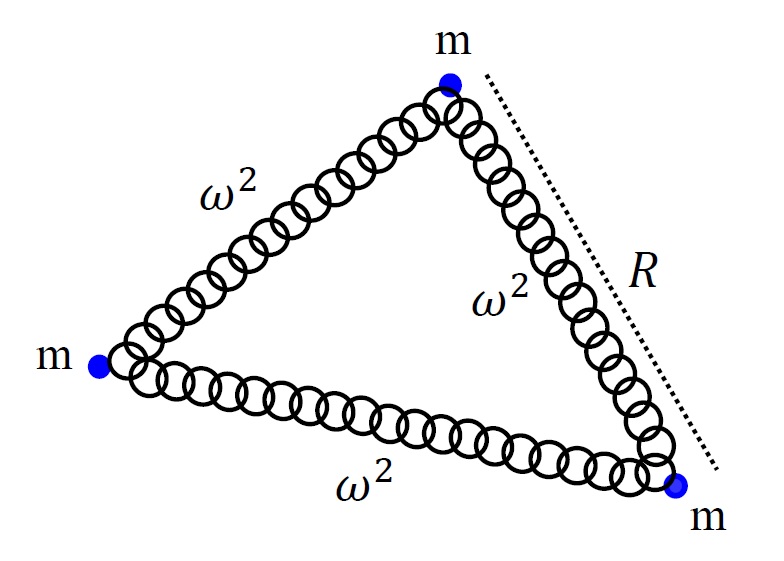
Figure 1: 3-body chain of harmonic oscillators. At the minimum of the potential $V_{R}$ (1), the system forms an equilateral triangle with sides $r_{12}=r_{13}=r_{23}=R$.

The Hamiltonian of the system is given by

$${\cal H}\ =\ \frac{1}{2\,m}{\hat{\mathbf{p}}_{{}_{1}}}^{2}\ +\ \frac{1}{2\,m}{\hat{\mathbf{p}}_{{}_{2}}}^{2}\ +\ \frac{1}{2\,m}{\hat{\mathbf{p}}_{{}_{3}}}^{2}\ +\ V_{R}(r_{ij})\ ,$$ (2)

here ${\hat{\mathbf{p}}_{{}_{j}}}=-i\,\hbar\,\nabla_{j}$ stands for the canonical momentum operator associated with the particle $j$. Due to translational invariance and rotational symmetry, the center of mass momentum

$${\hat{\mathbf{P}}}\ =\ {\hat{\mathbf{p}}_{{}_{1}}}\ +\ {\hat{\mathbf{p}}_{{}_{2}}}\ +\ {\hat{\mathbf{p}}_{{}_{3}}}\ ,$$ (3)

as well as the total angular momentum

$${\hat{\mathbf{L}}}\ =\ {\mathbf{r}}_{1}\times{\hat{\mathbf{p}}_{{}_{1}}}\ +\ {\mathbf{r}}_{2}\times{\hat{\mathbf{p}}_{{}_{2}}}\ +{\mathbf{r}}_{3}\times\ {\hat{\mathbf{p}}_{{}_{3}}}\ ,$$ (4)

are conserved quantities, respectively, i.e. they commute with the Hamiltonian (2). The corresponding stationary Schrödinger equation

$${\cal H}\,\Psi({\mathbf{r}}_{1},\,{\mathbf{r}}_{2},\,{\mathbf{r}}_{3})\ =\ E\,\Psi({\mathbf{r}}_{1},\,{\mathbf{r}}_{2},\,{\mathbf{r}}_{3})\ ,$$ (5)

is 9-dimensional.

Some remarks are in order:

• At $R=0$, the Hamiltonian ${\cal H}$ (2) admits a complete separation of variables in Jacobi coordinates de Castro and Sugaya (1993), see below. This separability holds even for the case of non-equal masses. Moreover, when all three masses are equal then the system becomes maximally superintegrable and exactly solvable Turbiner et al. (2020a). It is worth mentioning that for the same solvable model when restricted to a subdomain of the original configuration space, the supersymmetrization (SUSY realization) immediately encounters subtle difficulties Znojil (2003).

• For $R\neq 0$, not a singly exact solution to the Schrödinger equation is known so far. Interestingly, the corresponding classical system exhibits a rich dynamics with mixed regions of regularity and chaos Escobar-Ruiz et al. (2022).

The integrals of motion (3)-(4) allows us to construct a reduced Hamiltonian which describes all the states of ${\cal H}$ (2) with zero total angular momentum $L=0$ ($S$-states). It solely depends on the three variables $r_{ij}$ Turbiner et al. (2017). Explicitly, such a reduced Hamiltonian reads

$${\cal H}_{L=0}\ =\ -\frac{1}{2\,m}\triangle_{\rm rad}\ +\ \frac{3}{2}\,m\,\omega^{2}\,\left[{(r_{12}-R)}^{2}\,+\,{(r_{13}-R)}^{2}\,+\,{(r_{23}-R)}^{2}\right]\ ,$$ (6)

where the kinetic-like term can be written as follows:

$$\begin{split}&\frac{1}{2}\triangle_{\rm rad}\ =\ \frac{1}{r_{12}^{2}}\frac{\partial}{\partial r_{12}}\left(r_{12}^{2}\frac{\partial}{\partial r_{12}}\right)\ +\ \frac{1}{r_{13}^{2}}\frac{\partial}{\partial r_{13}}\left(r_{13}^{2}\frac{\partial}{\partial r_{13}}\right)\ +\ \frac{1}{r_{23}^{2}}\frac{\partial}{\partial r_{23}}\left(r_{23}^{2}\frac{\partial}{\partial r_{23}}\right)\ +\ \\ &\frac{r_{12}^{2}+r_{13}^{2}-r_{23}^{2}}{2\,r_{12}\,r_{13}}\,\frac{\partial^{2}}{\partial r_{12}\,\partial r_{13}}\ +\ \frac{r_{12}^{2}+r_{23}^{2}-r_{13}^{2}}{2\,r_{12}\,r_{23}}\,\frac{\partial^{2}}{\partial r_{12}\,\partial r_{23}}\ +\ \frac{r_{23}^{2}+r_{13}^{2}-r_{12}^{2}}{2\,r_{23}\,r_{13}}\,\frac{\partial^{2}}{\partial r_{23}\,\partial r_{13}}\ ,\end{split}$$ (7)

with $\hbar=1$, see Turbiner et al. (2018) and references therein. The operator (6) describes a 3-dimensional point particle moving in a (curved) space Turbiner et al. (2017). For the $S-$states, the relevant spectral problem occurs in the 3-dimensional space of radial relative motion ${\mathbb{R}}_{\rm rad}=(r_{12},r_{13},r_{23})\in{\mathbb{R}}^{3}_{+}$

$${\cal H}_{L=0}\,\psi(r_{12},r_{13},r_{23})\ =\ E\,\psi(r_{12},r_{13},r_{23})\ .$$ (8)

At $R=0$, the Hamiltonian (6) is $\mathbb{Z}_{2}^{\otimes 3}$-invariant under the reflections

$$r_{12}\rightarrow-r_{12}\quad;\qquad r_{13}\rightarrow-r_{13}\quad;\qquad r_{23}\rightarrow-r_{23}\ ,$$

and also under the action of the ${\mathcal{S}}_{3}^{\otimes 2}={\mathcal{S}}_{3}(r_{12},r_{13},r_{13})\oplus{\mathcal{S}}_{3}(1,2,3)$ symmetry (permutation of the three variables $r_{12},r_{13},r_{13},$ and interchange of any pair of particles). In the case $R\neq 0$, the discrete symmetry $\mathbb{Z}_{2}^{\otimes 3}$ is absent.

The Hamiltonian (6) is essentially self-adjoint with respect to the measure

$$d^{3}r\ =\ 8\,\pi^{2}\,r_{12}\,r_{13}\,r_{23}\,dr_{12}\,dr_{13}\,dr_{23}\ .$$ (9)

Accordingly, the configuration space ${\mathbb{R}}_{\rm rad}=(r_{12},r_{13},r_{23})$ is defined by the inequality $S\geq 0$ (see Figure 2), where $S$ is the area of the triangle formed by the three masses. Explicitly, using Heron’s formula, the area (squared) $S^{2}$ reads

$$S^{2}\ =\ \frac{1}{16}\,(r_{12}+r_{13}+r_{23})(r_{12}+r_{13}-r_{23})(r_{12}-r_{13}+r_{23})(-r_{12}+r_{13}+r_{23})\ .$$

Scaling Relation

The 3 parameters ($m,\,\omega,\,R$) in (6) define completely the harmonic 3-body system. Interestingly, one can relate two different systems ($m,\,\omega,\,R$) and ($m^{\prime},\,\omega^{\prime},\,R^{\prime}$) by making the scale transformation $r_{ij}\rightarrow\sqrt{\frac{m^{\prime}\,\omega^{\prime}}{m\,\omega}}\,r_{ij}$. That way, the following simple scaling relation between the two corresponding energies holds

$$E[m,\,\omega,\,R]\ =\ \frac{\omega}{\omega^{\prime}}\,E\bigg{[}m^{\prime},\,\omega^{\prime},\,R^{\prime}=\sqrt{\frac{m\,\omega}{m^{\prime}\,\omega^{\prime}}}\,R\bigg{]}\ .$$ (10)

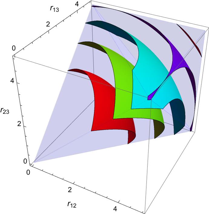
Figure 2: The domain $S\geq 0$ (shadow region), in the space of relative motion ${\mathbb{R}}_{\rm rad}=(r_{12},r_{13},r_{23})\in{\mathbb{R}}^{3}_{+}$, for the harmonic potential $V_{R}$ (1) with $m\,\omega^{2}=2/3$ and unit rest length $R=1$ a.u. The other surfaces (in color) correspond to level surfaces of $V_{R}$ (equipotentials).

III Case $R=0$: exact solutions

III.1 Jacobi-representation

Let us consider the original Hamiltonian ${\cal H}$ (2) which, by taking $R=0$, becomes

$${\cal H}\ =\ \frac{1}{2\,m}{\hat{\mathbf{p}}_{{}_{1}}}^{2}\ +\ \frac{1}{2\,m}{\hat{\mathbf{p}}_{{}_{2}}}^{2}\ +\ \frac{1}{2\,m}{\hat{\mathbf{p}}_{{}_{3}}}^{2}\ +\ \frac{3}{2}\,m\,\omega^{2}\,\left[r_{12}^{2}\,+\,r_{13}^{2}\,+\,r_{23}^{2}\right]\ .$$ (11)

This Hamiltonian (11) admits a complete separation of variables in Jacobi coordinates de Castro and Sugaya (1993); Turbiner et al. (2020a); Delves (1960). In the center-of-mass reference frame it takes the form

$${\cal H}\ =\ -\frac{1}{2}\bigg{[}\,\frac{\partial^{2}}{\partial{{\bf r}_{1}^{(J)}}\partial{{\bf r}_{1}^{(J)}}}\ +\ \frac{\partial^{2}}{\partial{{\bf r}_{2}^{(J)}}\partial{{\bf r}_{2}^{(J)}}}\,\bigg{]}\ +\ \frac{9}{2}\,\omega^{2}\,{{({\bf r}_{1}^{(J)}}}\cdot{{\bf r}_{1}^{(J)}})\ +\ \frac{9}{2}\,\omega^{2}\,{{({\bf r}_{2}^{(J)}}}\cdot{{\bf r}_{2}^{(J)}})\ ,$$ (12)

($\hbar=1$ and $m=1$) where

$${\bf r}^{(J)}_{1}\ =\ \sqrt{\frac{1}{2}}\left({\bf r}_{1}\ -\ {\bf r}_{2}\right),\qquad{\bf r}^{(J)}_{2}\ =\ \sqrt{\frac{2}{3}}\left({\bf r}_{3}\ -\ \frac{{\bf r}_{1}+{\bf r}_{2}}{2}\right)$$

are nothing but the two 3-dimensional vector Jacobi coordinates. In these variables, the Hamiltonian (11) corresponds to the sum of two identical 3-dimensional isotropic harmonic oscillators, more precisely, of two Jacobi harmonic oscillators Turbiner et al. (2020a). Hence, the system is maximally superintegrable and exactly solvable. In particular, in this Jacobi-representation the second quantization formalism in terms of creation and annihilation operators, namely

$${\cal H}\ =\ \sum_{\alpha}a^{\dagger}_{\alpha}\,a_{\alpha}\ +\ 9\,\omega\ ,$$ (13)

($\alpha$ is an index of a number of quantum numbers) can be introduced immediately. As demonstrated in Turbiner et al. (2020b), there exists a connection between the theory of superintegrable 2-dimensional systems (on the plane) and the theory of superintegrable systems (on the space of relative motion) of the 3-body problem parameterized by Jacobi distances. The spectra $E$ of (11) is the sum of spectra of individual Jacobi oscillators

$$E\ =\ \Lambda_{1}\ +\ \Lambda_{2}\ \equiv\ 3\,\omega\,\big{(}\,2\,[n_{1}\,+\,n_{2}]\ +\ell_{1}\ +\ \ell_{2}\ +\ 3\,\big{)}\ ,$$ (14)

and its eigenfunctions are the product

$$\Psi({\bf r}^{(J)}_{1},\,{\bf r}^{(J)}_{2})\ =\ \Psi_{1}^{(J)}({\bf r}^{(J)}_{1})\times\Psi_{2}^{(J)}({\bf r}^{(J)}_{2})\ ,$$ (15)

of the well-known individual solutions, see below. In spherical coordinates, ${\bf r}^{(J)}_{k}\equiv(r^{(J)}_{k},\,\theta^{(J)}_{k},\,\phi^{(J)}_{k})$, they are given by

$$\Psi_{k}^{(J)}({\bf r}^{(J)}_{k};\,n_{k},\,\ell_{k})\ =\ {\tau_{k}}^{\frac{\ell_{k}}{2}}\,e^{-\frac{3\,\omega}{2}\,\tau_{k}}\,L_{n_{k}}^{\ell_{k}+\frac{1}{2}}(3\,\omega\,\tau_{k})\,\,Y_{\ell_{k},\,s_{k}}(\theta^{(J)}_{k},\,\phi^{(J)}_{k})\,,\qquad k=1,2\ ,$$ (16)

where $\tau_{k}={(r^{(J)}_{k})}^{2}$, $\,L_{n_{k}}^{\ell_{k}+\frac{1}{2}}(3\,\omega\,\tau_{k})$ is a generalized Laguerre polynomial and $Y_{\ell_{k},\,s_{k}}$ denotes a spherical harmonic function. In (14)-(16), $n_{k}$ and $\ell_{k}$ are the individual radial and angular-momentum quantum numbers, respectively, of the $k$th Jacobi oscillator. In this representation the eigenfunctions of the Hamiltonian (12) are labeled by six quantum integers numbers ($n_{1},\,\ell_{1},\,s_{1};\,n_{2},\,\ell_{2},\,s_{2}$).

In the subspace of fixed $\ell_{1}$ and $\ell_{2}$, the Hamiltonian (12) reduces to

$${\cal H}\ =\ -\frac{1}{2}\sum_{k=1}^{2}\bigg{[}\,\frac{\partial^{2}}{\partial{{r}_{k}^{(J)}}\partial{{r}_{k}^{(J)}}}\ +\ \frac{2}{{r}_{k}^{(J)}}\frac{\partial}{\partial{{r}_{k}^{(J)}}}\ +\ \frac{\ell_{k}\,(\ell_{k}+1)}{{\big{(}{r}_{k}^{(J)}\big{)}}^{2}}\,\bigg{]}\ +\ \frac{9}{2}\,\omega^{2}\,\big{[}\,{\big{(}{r}_{1}^{(J)}\big{)}}^{2}\ +\ {\big{(}{r}_{2}^{(J)}\big{)}}^{2}\,\big{]}\ .$$ (17)

It acts on the $2$-dimensional space (${r}_{1}^{(J)},\,{r}_{2}^{(J)}$) of radial Jacobi distances alone. Evidently, it possesses a hidden Lie algebra $sl_{2}^{\,\otimes\,{2}}$.

Moreover, for fixed $\ell_{1}$ and $\ell_{2}$ the zero total angular momentum solutions ($S$-states) of the system are characterized by $\ell_{1}=\ell_{2}\equiv\ell$, $s_{1}=-s_{2}$ with $n_{1},n_{2}$ arbitrary. Otherwise in (12) the sum of the individual angular momentum of the two Jacobi oscillators is always different from zero. In the case $\ell_{1}=\ell_{2}\equiv\ell$ with $s_{1}=s_{2}=0$ it can be shown that the degeneracy of the $N$th-level $E=3\,\omega\,(2N+3)$, with $N=n_{1}+n_{2}+\ell$, is $g=\frac{(N+1)(N+2)}{2}$.

III.2 $\rho$-representation

If we now consider the reduced Hamiltonian ${\cal H}_{L=0}$ in (8), it is found that at $R=0$ it admits special solutions in the factorized form

$$\psi^{(g)}_{N}\ =\ P_{N,g}(r_{12}^{2},\,r_{13}^{2},\,r_{23}^{2})\times e^{-\frac{\omega}{2}(r_{12}^{2}+r_{13}^{2}+r_{23}^{2})}\ ,$$ (18)

where $P_{N,g}$ is a multivariate polynomial of degree $N$ in variables

$$\rho_{ij}\ =\ r_{ij}^{2}\,,\qquad\ i\neq j\,=\,1,2,3\ ,$$ (19)

and $g=(N+1)(N+2)/2$ is the degeneracy of the $N$th-level $E_{N}$

$$E_{N}\ =\ 3\,\omega\,\big{(}\,2\,N\ +\ 3\,\big{)}\,,\qquad N=0,1,2,3\ldots\ .$$ (20)

In these variables $\rho_{ij}=r_{ij}^{2}$, the Hamiltonian ${\cal H}_{L=0}$ in (8) possesses a hidden Lie algebra $sl_{4}$, and it can be rewritten (up to a gauge transformation) in terms of $sl_{4}$ algebra generators. The eigenvalues become linear in 3 quantum numbers Turbiner et al. (2020a), namely $N=N_{1}+N_{2}+N_{3}$. We emphasize that (8) does not separate in the $\rho-$variables.

In particular, for the normalized ground state $N=0$ eigenfunction we obtain

$$\psi_{0}\ =\ \frac{2\,\pi}{3\,\sqrt{3}\,\omega^{3}}e^{-\frac{\omega}{2}(\,\rho_{12}+\rho_{13}+\rho_{23}\,)}\ ,$$ (21)

with energy $E_{0}=9\,\omega$, whereas for the first excited state $N=1$ there exist 3 degenerate solutions of the form (18), explicitly they read

$$\begin{split}&\psi_{1}^{(0)}\ =\ \frac{(3)^{\frac{5}{4}}\omega^{\frac{3}{2}}}{\sqrt{2\,\pi}}\,(\,1\ -\ \omega\,\rho_{12})\,e^{-\frac{\omega}{2}(\,\rho_{12}+\rho_{13}+\rho_{23}\,)}\\ &\psi_{1}^{(1)}\ =\ \frac{(3)^{\frac{5}{4}}\omega^{\frac{3}{2}}}{\sqrt{2\,\pi}}\,(\,1\ -\ \omega\,\rho_{13})\,e^{-\frac{\omega}{2}(\,\rho_{12}+\rho_{13}+\rho_{23}\,)}\\ &\psi_{1}^{(2)}\ =\ \frac{(3)^{\frac{5}{4}}\omega^{\frac{3}{2}}}{\sqrt{2\,\pi}}\,(\,1\ -\ \omega\,\rho_{23})\,e^{-\frac{\omega}{2}(\,\rho_{12}+\rho_{13}+\rho_{23}\,)}\ ,\end{split}$$ (22)

corresponding to the same energy $E_{1}=15\,\omega$.

In this way, in the case $R=0$ we arrive to the following results:

• For the $S-$states of (12), the subset of the exact eigenfunctions $\Psi({\bf r}^{(J)}_{1},\,{\bf r}^{(J)}_{2})$ (15) in Jacobi coordinates characterized by $\ell_{1}=\ell_{2}=\ell$ and $s_{1}=s_{2}=0$ can be completely expressed as a linear combination of the $\rho$-dependable special solutions (18). To illustrate this point, for the lowest states $N=0,1,2$ we indicate, see Table 1, the degeneration of the system in both representations.

• The ground state eigenfunction of the original Hamiltonian (2) solely depends on the three $\rho-$variables, $\rho_{ij}=r^{2}_{ij}$, the three relative distances (squared). It is presented in (21).

• For the $S-$states of (12), the exact eigenfunctions $\Psi({\bf r}^{(J)}_{1},\,{\bf r}^{(J)}_{2})$ (15) in Jacobi coordinates characterized by $\ell_{1}=\ell_{2}=\ell$ but $s_{1}\neq s_{2}$ can not be expressed as a polynomial in $\rho-$variables multiplied by the ground state eigenfunction.

Table 1: $S-$states: Degeneration of the energy level $E_{N}=3\,\omega\,(\,2\,N\,+\,3\,)$ in (I) the Jacobi-representation ($N=n_{1}+n_{2}+\ell$) with $s_{1}=s_{2}=0$ vs (II) the $\rho-$representation ($N=N_{1}+N_{2}+N_{3}$).

$N$	$n_{1}$	$n_{2}$	$\ell$	$N_{1}$	$N_{2}$	$N_{3}$
0	0	0	0	0	0	0
1	1	0	0	1	0	0
1	0	1	0	0	1	0
1	0	0	1	0	0	1
2	2	0	0	2	0	0
2	0	2	0	0	2	0
2	1	1	0	0	0	2
2	1	0	1	1	1	0
2	0	1	1	1	0	1
2	0	0	2	0	1	1

It will be shown that for $R>0$ and fixed $N$, the original degenerate $g-$eigenfunctions with $g=\frac{(N+1)(N+2)}{2}$ split into $(N(N+1)+2)/2$ different energy sub-levels.

IV Case $R>0$: ground state

In this Section, as a first step we study the ground state of the spectral problem (8) as a function of the rest length $R$. To find the corresponding approximate solutions, the perturbative and the variational method are employed.

IV.1 Small $R$: perturbation theory

Taking the $R-$dependent terms in the potential $V_{R}$ (1) as a perturbation to the exactly solvable problem $V_{R=0}$, one can immediately compute the first correction to the energy within the non-linearization procedure Turbiner (1984). Putting $m=1$, the original potential $V_{R}$ (1) can be written as a sum of three terms

$$V_{R}\,=\,\frac{3}{2}\,\omega^{2}\,\left[r_{12}^{2}\,+\,r_{13}^{2}\,+\,r_{23}^{2}\right]\ -\ 3\,\omega^{2}\,R\,(r_{12}+r_{13}+r_{23})\ +\ \frac{9}{2}\,\omega^{2}\,R^{2}\ ,$$ (23)

where the first term corresponds to an exactly solvable potential whereas the last one is just a constant. Let us write the ground state function in exponential form:

$$\psi_{0}(r_{12},\,r_{13},\,r_{23}\,)\ =\ e^{-\Phi_{0}(r_{12},\,r_{13},\,r_{23}\,)}\ ,$$

here $\Phi$ is the phase of the wave function. Next, we develop perturbation theory in powers of $R$, namely

$$E_{0}\ =\ \sum_{n=0}^{\infty}\epsilon_{n}\,R^{n}\qquad;\qquad\Phi_{0}(\,r_{12},\,r_{13},\,r_{23}\,)\ =\ \sum_{n=0}^{\infty}a_{n}(r_{12},\,r_{13},\,r_{23}\,)\,R^{n}\ ,$$ (24)

with $\epsilon_{0}=9\,\omega$ and $a_{0}={\frac{\omega}{2}(r_{12}^{2}+r_{13}^{2}+r_{23}^{2})}$ being the exact ground- state solution occurring for $R=0$. As a result of direct calculations, we obtain the value

$$E_{0}(R)\ =\ 9\,\omega\ +\ \frac{3\,\omega}{2\,\pi}(\,3\,\pi\,\omega\,R^{2}\ -\ 4\,R\,\sqrt{6\,\pi\,\omega}\,)\ +\ {\rm corrections}\ .$$ (25)

Therefore, taking the zero and first order corrections as well as the constant term appearing in (23), perturbation theory predicts the existence of a global minimum in $E_{0}(R)$, localized at $R=R_{\rm crit}\sim 2\sqrt{\frac{2}{3\,\pi\,\omega}}$, which would corresponds to an equilateral configuration of equilibrium. Since this phenomenon could be an artifact of the deficiency of perturbation theory we will verify it using different approximate methods, see below.

IV.2 Arbitrary $R$: variational method

For arbitrary $R$, to evaluate the ground state energy $E_{0}(R)$ we take the simple two-parametric trial function

$$\psi_{\rm trial}\ =\ e^{-\frac{\alpha\,\omega}{2}\big{(}\,{(r_{12}\,-\,\beta\,R)}^{2}\ +\ {(r_{13}\,-\,\beta\,R)}^{2}\ +\ {(r_{23}\,-\,\beta\,R)}^{2}\,\big{)}}\ ,$$ (26)

where $\alpha,\,\beta\in[0,\,1]$ are variational parameters. At $\beta=0$ with $\alpha=1$, the function (26) degenerates into the exact solution appearing at $R=0$. Though the value of the minimum in $E_{0}(R)$ disagrees with that found in perturbation theory, the variational method also predicts the existence of a global minimum. At fixed $\omega=1$, a comparison of the values for $E_{0}(R)$ obtained with the perturbative (25), variational (using the optimal (26)) and Lagrange-mesh method (see below), respectively, is displayed in Figure 3 within the interval $R\in[0,\,3.5]$ a.u. In this case, perturbation theory (25) provides reasonable accurate results when $0\leq R\leq 0.3$ a.u. whereas for the variational method the corresponding interval of applicability is larger $0\leq R\leq 2.3$ a.u., as expected. A quantitative comparison between the variational and Lagrange-mesh results is presented in Table 2. In particular, the relative difference increases from $0.003\%$ at $R=0.2$ a.u. up to $9\%$ at $R=7/2$ a.u.

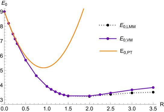
Figure 3: Comparison of the ground state energy $E_{0}$ in a.u. calculated using Perturbation Theory (PT) (25), the variational function $\psi_{\rm trial}$ (VM) (26) and the Lagrange-Mesh Method (LMM), see below, at $\omega=1$.

Table 2: Variational ground state energy $E_{0}^{\rm{VM}}$ vs $R$ computed using the 2-parametric trial function $\psi_{\rm trial}$ (26) with $\omega=1$. The optimal values of the parameters $\alpha$ and $\beta$ are also displayed. $E_{0}^{\rm{LMM}}$ corresponds to the value of the energy calculated using the Lagrange-mesh method (see below). The relative error (RE) is presented in the last column.

$R$	$E_{0}^{\rm{VM}}$	$\alpha$	$\beta$	$E_{0}^{\rm{LMM}}$	RE
0.0	9	1	0	9.000000000000	0
0.2	7.48081	0.960	0.300	7.480575209823	0.00003
0.3	6.82304	0.935	0.300	6.822630580417	0.00006
0.5	5.70206	0.875	0.310	5.700976066954	0.00019
1.0	3.92165	0.790	0.440	3.916842671126	0.00123
1.1	3.71684	0.770	0.460	3.710814446829	0.00162
1.2	3.55424	0.760	0.500	3.546619661941	0.00215
1.3	3.42955	0.760	0.544	3.420165435764	0.00274
1.4	3.33804	0.760	0.577	3.327196880347	0.00326
1.5	3.27597	0.760	0.610	3.263367579471	0.00386
2.0	3.26821	0.754	0.730	3.233525277971	0.01073
2.5	3.46849	0.750	0.843	3.373848351684	0.02805
3.0	3.68241	0.750	0.900	3.473009053896	0.06029
3.5	3.84142	0.750	0.930	3.522515737857	0.09053

V The Lagrange-mesh method

In order to solve the Schrödinger equation for the Hamiltonian (6), the Lagrange-mesh method (LMM) is also applied Baye and Heenen (1986); Baye (2015). To introduce this methodology let’s consider a one-dimensional problem where a set of $M$ Lagrange functions $f_{i}\,(x)$ defined over the domain $x\in[\,0,\infty)$ is associated with $M$ mesh points $x_{i}$ which correspond to the zeros of Laguerre polynomials of degree $M$, i.e. $L_{M}(x_{i})=0$. The Lagrange-Laguerre functions $f_{i}\,(x)$ which satisfy the Lagrange conditions

$$f_{i}(x_{j})=\lambda_{i}^{-1/2}\delta_{ij}\,,$$ (27)

at the $M$ mesh points are given by

$$f_{i}(x)=(-1)^{i}\frac{x}{x_{i}^{1/2}}\frac{L_{M}(x)}{(x-x_{i})}e^{-x/2}\,,$$ (28)

and the coefficients $\lambda_{i}$ are the weights associated with a Gauss quadrature

$$\int_{0}^{\infty}G(x)dx\approx\sum_{k=1}^{M}\lambda_{k}\,G(x_{k})\,.$$ (29)

In terms of the $M$ Lagrange functions $f_{i}(x)$ (28), the solution of the Schrödinger equation for a particle of mass $m$ in a potential $V(x)$ is expressed as

$$\psi(r)=\sum_{i=1}^{M}c_{i}f_{i}(r)\,.$$ (30)

The function (30), together with the Gauss quadrature (29) and the Lagrange conditions (27) leads to the system of variational equations

$$\sum_{j=1}^{M}\left[\frac{\hbar^{2}}{2m}\,T_{ij}+V(x_{i})\delta_{ij}\right]\,c_{j}=E\,c_{i}\,,$$ (31)

where $T_{ij}$ are the kinetic-energy matrix elements (see for example Baye (2015)) and $V(x_{i})$ is the potential evaluated at the mesh points $x_{i}$. By solving the system (31), the energies $E$ and the eigenvectors $c_{i}$ are obtained, from which the approximation to the wave function (30) is obtained.

The present system has three degrees of freedom which are described by the three distances between the particles: $r_{12}$, $r_{13}$ and $r_{23}$. Technically, a considerable simplification results from going over to the so-called perimetric coordinates used by Pekeris in his helium calculations Pekeris (1958). These perimetric coordinates are defined by the linear relations

$$x\ =\ r_{12}\ +\ r_{13}\ -\ r_{23}\,,$$ (32)

$$y\ =\ r_{12}\ -\ r_{13}\ +\ r_{23}\,,$$

$$z\ =\ -r_{12}\ +\ r_{13}\ +\ r_{23}\,.$$

The volume element is $dV\propto(x+y)(x+z)(y+z)dx\,dy\,dz$. By the above transformation the limits of the three perimetric coordinates $x$, $y$ and $z$ become independent of each other and they vary from $0$ to $\infty$.

In perimetric coordinates, following the notation presented in Baye and Dohet-Eraly (2015), the matrix elements of the kinetic energy operator (6) $\langle F|\hat{T}|G\rangle$ between functions $F$ and $G$ can be written as

$$\langle F|\hat{T}|G\rangle=\int_{0}^{\infty}\,dx\,\int_{0}^{\infty}\,dy\,\int_{0}^{\infty}\,dz\sum_{i,j=1}^{3}A_{ij}(x,y,z)\frac{\partial F}{\partial x_{i}}\frac{\partial G}{\partial x_{j}}\,,$$ (33)

where $(x_{1},x_{2},x_{3})=(x,y,z)$ and the coefficients $A_{ij}$ are given by

$$A_{1,1} = x(y+z)(x+y+z)+xz(x+z)+xy(x+y)\,,$$ (34)

$$A_{2,2} = yz(y+z)+y(x+z)(x+y+z)+xy(x+y)\,,$$

$$A_{3,3} = yz(y+z)+xz(x+z)+z(x+y)(x+y+z)\,,$$

$$A_{1,2} = A_{2,1}=-xy(x+y)\,,$$

$$A_{1,3} = A_{3,1}=-xz(x+z)\,,$$

$$A_{2,3} = A_{3,2}=-yz(y+z)\,.$$

The generalization of the Lagrange-mesh method to the three-dimensional case is as follows Hesse and Baye (2001, 2003). The three-dimensional Lagrange functions $F_{ijk}(x,y,z)$ are defined as

$$F_{ijk}(x,y,z)={\cal N}_{ijk}^{-1/2}f_{i}^{M_{x}}(x/h_{x})f_{j}^{M_{y}}(y/h_{y})f_{k}^{M_{z}}(z/h_{z})\,,$$ (35)

where the functions $f_{i}^{M}$ all have the same structure as (28) with $M$ replaced by the respective degrees $M_{x}$, $M_{y}$ and $M_{z}$ and the zeros $x_{p}$ ($p=1,...,M_{x}$), $y_{q}$ ($q=1,...,M_{y}$) and $z_{r}$ ($r=1,...,M_{z}$) are the zeros of the respective Laguerre polynomials. The scaling parameters $h_{x}$, $h_{y}$ and $h_{z}$ are incorporated to fit the mesh to the physical system. The normalization factor ${\cal N}_{ijk}$ is defined by

$${\cal N}_{ijk}=h_{x}\,h_{y}\,h_{z}\,(h_{x}\,x_{i}+h_{y}\,y_{j})(h_{x}\,x_{i}+h_{z}\,z_{k})(h_{y}\,y_{j}+h_{z}\,z_{k})\,.$$ (36)

This three-dimensional Lagrange functions (35) satisfy

$$F_{ijk}(h_{x}\,x_{i^{\prime}},h_{y}\,y_{j^{\prime}},h_{z}\,x_{k^{\prime}})=({\cal N}_{ijk}\,\lambda_{i}\,\mu_{j}\,\nu_{k})^{-1/2}\,\delta_{ii^{\prime}}\delta_{jj^{\prime}}\delta_{kk^{\prime}}\,,$$ (37)

where $\lambda_{i}$, $\mu_{j}$ and $\nu_{k}$ are the weights of the Gauss quadratures (29) for the variables $x$, $y$ and $z$, respectively. In terms of the Lagrange functions $F_{ijk}(x,y,z)$ (35), the wave function is expanded as

$$\Psi(x,y,z)=\sum_{i=1}^{M_{x}}\sum_{j=1}^{M_{y}}\sum_{k=1}^{M_{z}}C_{ijk}F_{ijk}(x,y,z)\,,$$ (38)

which makes it possible, together with the Gauss quadratures for each variable and condition (37), to write the Schrodinger equation for the Hamiltonian (6) as a mesh equation

$$\sum_{i=1}^{M_{x}}\sum_{j=1}^{M_{y}}\sum_{k=1}^{M_{z}}\left\{\langle F_{i^{\prime}j^{\prime}k^{\prime}}|T|F_{ijk}\rangle+[\langle F_{i^{\prime}j^{\prime}k^{\prime}}|V|F_{ijk}\rangle-E]\delta_{ii^{\prime}}\delta_{jj^{\prime}}\delta_{kk^{\prime}}\right\}C_{ijk}=0\,.$$ (39)

The matrix elements of the potential $\langle F_{i^{\prime}j^{\prime}k^{\prime}}|V|F_{ijk}\rangle$ have a very simple representation

$$\langle F_{i^{\prime}j^{\prime}k^{\prime}}|V|F_{ijk}\rangle=V(h_{x}\,x_{i},h_{y}\,y_{i},h_{z}\,z_{i})\,\delta_{ii^{\prime}}\,\delta_{jj^{\prime}}\,\delta_{kk^{\prime}}\,,$$ (40)

which correspond to the potential $V_{R}$ (1) in perimetric coordinates evaluated at the mesh points. In contrast, the matrix elements of the kinetic energy operator $\langle F_{i^{\prime}j^{\prime}k^{\prime}}|T|F_{ijk}\rangle$ between two elements $F_{ijk}$ (33) are given by

$$\langle F_{i^{\prime}j^{\prime}k^{\prime}}|T|F_{ijk}\rangle = 2\,{\cal N}_{i^{\prime}j^{\prime}k^{\prime}}^{-1/2}\,{\cal N}_{ijk}^{-1/2}\,h_{x}\,h_{y}\,h_{z}\,\left\{\right.$$

$$\delta_{jj^{\prime}}\,\delta_{kk^{\prime}}\,\sum_{n}\lambda_{n}\,h_{x}^{-2}\,A_{11}(h_{x}x_{n},h_{y}y_{j},h_{z}z_{k})\,f^{\prime}_{i}(x_{n})\,f^{\prime}_{i^{\prime}}(x_{n})$$

$$+ \delta_{ii^{\prime}}\,\delta_{kk^{\prime}}\,\sum_{n}\mu_{n}\,h_{y}^{-2}\,A_{22}(h_{x}x_{i},h_{y}y_{n},h_{z}z_{k})\,f^{\prime}_{j}(y_{n})\,f^{\prime}_{j^{\prime}}(y_{n})$$

$$+ \delta_{ii^{\prime}}\,\delta_{jj^{\prime}}\,\sum_{n}\nu_{n}\,h_{z}^{-2}\,A_{33}(h_{x}x_{i},h_{y}y_{j},h_{z}z_{n})\,f^{\prime}_{k}(z_{n})\,f^{\prime}_{k^{\prime}}(z_{n})$$

$$+ \delta_{kk^{\prime}}(h_{x}\,h_{y})^{-1}[(\lambda_{i}\mu_{j^{\prime}})^{1/2}\,A_{12}(h_{x}\,x_{i},h_{y}\,y_{j^{\prime}},h_{z}\,z_{k})\,f^{\prime}_{i^{\prime}}(x_{i})\,f^{\prime}_{j}(y_{j^{\prime}})$$

$$\hskip 59.75095pt+(\lambda_{i^{\prime}}\mu_{j})^{1/2}\,A_{12}(h_{x}\,x_{i^{\prime}},h_{y}\,y_{j},h_{z}\,z_{k})\,f^{\prime}_{i}(x_{i^{\prime}})\,f^{\prime}_{j^{\prime}}(y_{j})]$$

$$+ \delta_{jj^{\prime}}(h_{x}\,h_{z})^{-1}[(\lambda_{i}\nu_{k^{\prime}})^{1/2}\,A_{13}(h_{x}\,x_{i},h_{y}\,y_{j},h_{z}\,z_{k^{\prime}})\,f^{\prime}_{i^{\prime}}(x_{i})\,f^{\prime}_{k}(z_{k^{\prime}})$$

$$\hskip 56.9055pt+(\lambda_{i^{\prime}}\nu_{k})^{1/2}\,A_{13}(h_{x}\,x_{i^{\prime}},h_{y}\,y_{j},h_{z}\,z_{k})\,f^{\prime}_{i}(x_{i^{\prime}})\,f^{\prime}_{k^{\prime}}(z_{k})]$$

$$+ \delta_{ii^{\prime}}(h_{y}\,h_{z})^{-1}[(\mu_{j}\nu_{k^{\prime}})^{1/2}\,A_{23}(h_{x}\,x_{i},h_{y}\,y_{j},h_{z}\,z_{k^{\prime}})\,f^{\prime}_{j^{\prime}}(y_{j})\,f^{\prime}_{k}(z_{k^{\prime}})$$

$$\hskip 56.9055pt+(\mu_{j^{\prime}}\nu_{k})^{1/2}\,A_{23}(h_{x}\,x_{i},h_{y}\,y_{j^{\prime}},h_{z}\,z_{k})\,f^{\prime}_{j}(y_{j^{\prime}})\,f^{\prime}_{k^{\prime}}(z_{k})]\left.\right\}\,,$$

with the coefficients $A_{ij}$ defined by (V) and $f^{\prime}_{i}(x_{j})=df_{i}(x)/dx|_{x=x_{j}}$ and analogously for $y$ and $z$. To obtain the solution of the mesh equation (40), we consider $M_{x}=M_{y}=M_{z}=M$ and $h_{x}=h_{y}=h_{z}=h$. The so obtained results are presented in the following section.

VI Results and discussion

In this Section the energies $E=E(R)$ appearing in (8) for the lowest $S$-states solutions $\psi(x,y,z)$ (38) using the Lagrange-mesh method are presented. For clarity of the degeneracy as a function of $R$, the energies are denoted by $E=E_{N,n}$. At $R=0$ a.u. the label $N$ corresponds to the quantum number of the exact solution (18). For $R>0$, the degenerate $N$th-level splits into sub-levels denoted by $n=0,1,2,3,\ldots$.

Table 3 presents the energy values for $\omega=0.5$ and $R\in[0.0,4.0]$ a.u. in constant steps of $0.5$ a.u. for four different values of $N$: $N=0,1,2$ and $3$. In all cases 12 decimal digits are provided. The limit case $R=0$, presented in the second column, is in complete agreement with the analytic solution (20). It can also be noticed that the degeneracy obtained for each $N$ value $g_{0}=1$, $g_{1}=3$, $g_{2}=6$ and $g_{3}=10$ for $N=0,1,2$ and $3$, respectively, coincides with the values of the analytic expression $g_{N}=(N+1)(N+2)/2$. For $R\neq 0$, the degeneration is partially removed: each $g_{N}$-degenerated energetic level $E_{N}$ seems to unfold into $(N(N+1)+2)/2$ different energy levels $E_{N,n}$, as can be seen in columns $3$ through $6$ of Table 3 (and its continuation) and Figure 4 where the results are depicted. As pointed out in the previous sections for the case $\omega=1.0$ (see also below), the ground state $E_{0,0}$ presents a minimum. For $\omega=0.5$ the equilibrium length for which the minimum appears is $R_{min}\approx 2.494583$ a.u. and the corresponding energy value is $E_{0,0}^{min}=1.601390190475$ a.u. A global minimum in energy as a function of $R$ is present for excited states $E_{N,n}$ as well.

Similar calculations were carried out for the case $\omega=1.0$ for $R\in[0.0,6.0]$ a.u. in constant steps of $0.5$ a.u. for three values of $N$: $N=0,1$ and $2$. These are depicted in Figure 5. The position of the minimum for the ground state $E_{0,0}$ present in Figure 3, appears for a rest length of $R_{min}\approx 1.763936$ a.u. and the energy value is $E_{0,0}^{min}=3.202780380949$ a.u.

Results presented in Table 3 for the system defined by the parameters $(m,w,R)=(1,1/2,R)$ allow us, according to the scaling relation (10), to obtain the spectrum for the system defined by the parameters $(m^{\prime},w^{\prime},R^{\prime})$ as

$$E\bigg{[}m^{\prime},\,\omega^{\prime},\,R^{\prime}=\sqrt{\frac{1}{2\,m^{\prime}\,\omega^{\prime}}}\,R\bigg{]}=2\,\omega^{\prime}\,E[m=1,\,\omega=1/2,\,R]\,.$$ (42)

Likewise, for fixed $m$ and $\omega$ it can be shown that the energy tends asymptotically to a finite value at large $R$, namely $E[m,\,\omega,\,R\rightarrow\infty]\rightarrow E_{\infty}$ with $0<E_{\infty}<E[m,\,\omega,\,R=0]$.

Table 3: Energy $E_{N,n}$ in a.u. of the three-body system with harmonic interactions for four values of $N=0,1,2,3$. Results for 11 rest lengths $R$ are presented for $m=1$ and $\omega=0.5$.

$N,n$	$R=0.0$      .	$R=0.5$      .	$R=1.0$	$R=1.5$	$R=2.0$
0,0	4.500000000000	3.248654270738	2.398230674763	1.893326994351	1.658224669986
1,0	7.500000000000	5.822579071286	4.556769365814	3.664863226784	3.097422523508
1,0	7.500000000000	5.822579071286	4.556769365814	3.664863226784	3.097422523508
1,1	7.500000000000	5.888219366854	4.698676482022	3.894470971731	3.420048994408
2,0	10.500000000000	8.425989881143	6.767207301164	5.497092599573	4.585730111853
2,1	10.500000000000	8.478177133040	6.875163036857	5.662422650165	4.803713591948
2,1	10.500000000000	8.478177133040	6.875163036857	5.662422650165	4.803713591948
2,2	10.500000000000	8.545207941409	7.012948079404	5.872301106010	5.080840901420
2,2	10.500000000000	8.545207941409	7.012948079404	5.872301106010	5.080840901420
2,3	10.500000000000	8.585804667998	7.102564535323	6.022347722884	5.304426211111
3,0	13.500000000000	11.117248579552	9.151798562159	7.580579295969	6.377989183868
3,0	13.500000000000	11.117248579552	9.151798562159	7.580579295969	6.377989183868
3,1	13.500000000000	11.166486177781	9.256862108632	7.749845695543	6.621624051144
3,2	13.500000000000	11.182671178672	9.286960974298	7.788519430823	6.657403147017
3,3	13.500000000000	11.201333020368	9.327772383811	7.855960948738	6.756193130417
3,4	13.500000000000	11.237400167902	9.401828686849	7.969149439956	6.907794387450
3,4	13.500000000000	11.237400167902	9.401828686849	7.969149439956	6.907794387450
3,5	13.500000000000	11.299682142132	9.527870507574	8.157727630210	7.152137692085
3,5	13.500000000000	11.299682142132	9.527870507574	8.157727630210	7.152137692085
3,6	13.500000000000	11.323644849540	9.581929109473	8.251164113636	7.298585516817
continued …

Table 3: Continued.

$N,n$	$R=2.5$	$R=3.0$	$R=3.5$	$R=4.0$
0,0	1.601395264863	1.632400069954	1.683574737362	1.723086021257
1,0	2.792200036372	2.676557025969	2.674697030516	2.718769132833
1,0	2.792200036372	2.676557025969	2.674697030516	2.718769132833
1,1	3.190836945883	3.103332798190	3.091624824311	3.131015526880
2,0	4.001306153939	3.700994915894	3.599821980119	3.598727725394
2,1	4.252422060901	3.946997916389	3.809333229038	3.770583846482
2,1	4.252422060901	3.946997916389	3.809333229038	3.770583846482
2,2	4.579692643406	4.292955936169	4.152251395868	4.120366124525
2,2	4.579692643406	4.292955936169	4.152251395868	4.120366124525
2,3	4.884422564011	4.669310533464	4.577280487589	4.566099117819
3,0	5.518635696594	4.979122899313	4.716809070758	4.632409629401
3,0	5.518635696594	4.979122899313	4.716809070758	4.632409629401
3,1	5.846087784304	5.343189633908	5.062981319388	4.902633799079
3,2	5.857032828332	5.382348879247	5.105850276064	4.953740120564
3,3	5.988214691550	5.494885196598	5.235209305583	5.158583646230
3,4	6.173864755693	5.701271082276	5.401007220296	5.222212371602
3,4	6.173864755693	5.701271082276	5.401007220296	5.222212371602
3,5	6.458573386971	6.007877096278	5.730592301379	5.579591036652
3,5	6.458573386971	6.007877096278	5.730592301379	5.579591036652
3,6	6.675266892942	6.308388406757	5.857172620421	5.654200458590

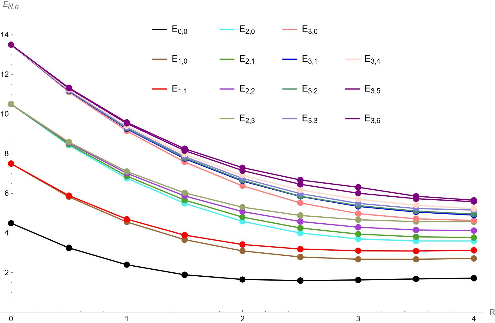
Figure 4: The energy $E_{N,n}$ vs $R$ of the three-body harmonic system $V_{R}$ (1) for the 14 lowest $S$-states. It is a smooth function of $R$. Numerical values calculated with the Lagrange-Mesh method are marked by bullets, the lines are a guide to the eye. The values $m=1$ and $\omega=1/2$ were used in the calculations (color online). Energy is presented in Hartrees.

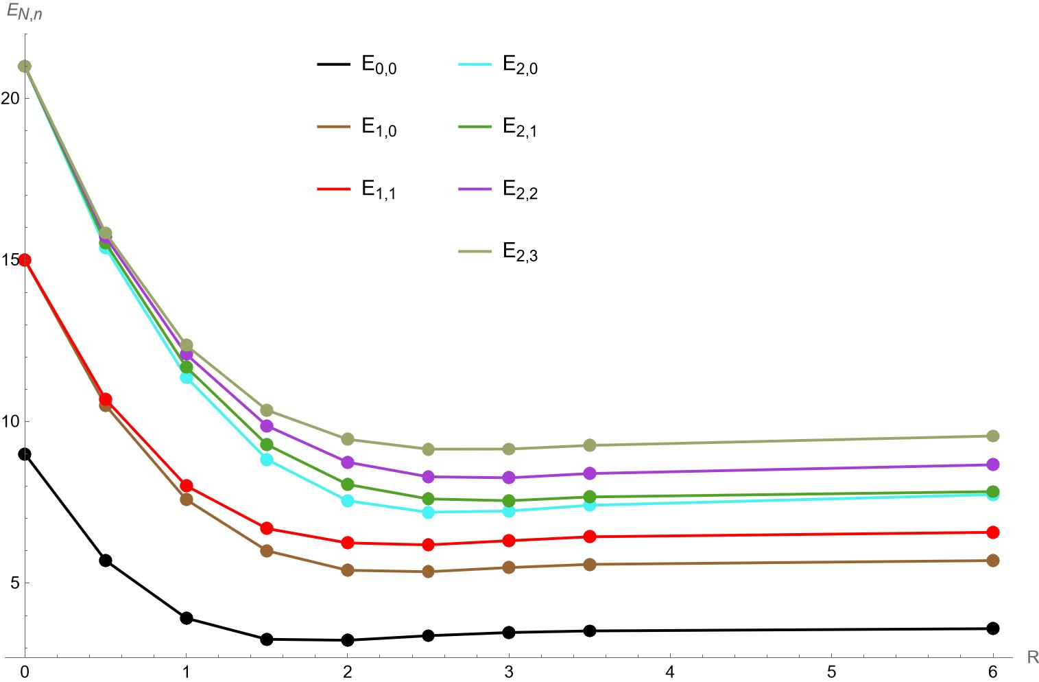
Figure 5: The energy $E_{N,n}$ vs $R$ of the three-body harmonic system $V_{R}$ (1) for the 7 lowest $S$-states with parameters $m=1$ and $\omega=1$. It is a smooth function of $R$. Numerical values calculated with the Lagrange-Mesh method are marked by bullets, the lines are a guide to the eye (color online). Energy is presented in Hartrees.

Now, in the case of 3 particles with arbitrary masses and inspired by a phenomenological model of the forces inside a baryon where 3 quarks are connected by 3 glue strings and these strings meet at a “gluon junction” (see Alexandrou et al. (2003) and references therein), one can also consider a generalization of (1) given by

$${\tilde{V}}_{R}\,\equiv\,\frac{3}{2}\,\omega^{2}\,\left[{\nu_{12}\,(r_{12}-R_{12})}^{2}\,+\,\nu_{13}\,{(r_{13}-R_{13})}^{2}\,+\nu_{23}\,\,{(r_{23}-R_{23})}^{2}\right]\ ,$$ (43)

where $\nu_{ij}$ are parameters (not all of them necessarily positive) and the rest lengths $R_{ij}>0$ can take different values. Such a model can play an important role in molecular and atomic 3-body systems where the configuration of equilibrium corresponds to a triangular one ( for instance the H${}_{3}^{+}$ ion Kutzelnigg and Jaquet (2006)). In this case, at $R_{12}=R_{13}=R_{23}=0$ the system is separable and exactly-solvable again de Castro and Sugaya (1993) for any value of the conserved total angular momentum.

VII Conclusions

For the generalized 3-body harmonic system the energies of the first 14 lowest $S-$states were computed with accuracy of 11 figures in the domain of $R\in[0.0,\,4.0]$ a.u. . At $R=0$, the problem becomes maximally superintegrable and exactly solvable. The corresponding degenerate levels were analyzed in two-different Lie-algebraic representations. At $R>0$, in order to solve the Schrodinger equation for this three-body system (8), three methods were implemented for the ground state: $i$) the perturbation method (PT), $ii$) the variational method (VM) and $iii$) the Lagrange-mesh method (LMM). The first two (PT and VM) indicated the presence of a global minimum in the ground state energy for a certain value of $R=R_{\rm min}>0$, which was precisely confirmed by the LMM. In all cases the energy $E(R)$ of the lowest states as a function of $R$ displays a smooth behavior (Figures 4 and 5). The degeneracy of the system when $R=0$ is partially removed for $R>0$, and the quantitative splitting of levels was presented. Making an evident modification of the Hamiltonian (2) the analogue 3-body generalized harmonic system can be written for arbitrary masses and different spring constants (43). Such a model can serve as a zero order approximation for the study of 3-body Coulomb atomic and molecular systems. We plan to address this subject in future studies. It is also worth mentioning that within the LMM it is possible and straightforward to consider states with non-zero angular momentum, $i.e.$ states with $L\neq 0$.

DATA AVAILABILITY

Data sharing is not applicable to this article as no new data were created or analyzed in this study.

Author information

These authors contributed equally: A. M. Escobar-Ruiz and H. Olivares-Pilón.

Competing interests

The authors declare no competing interests.

References

- Moshinsky and Smirnov (1996) M. Moshinsky and Y. Smirnov, The Harmonic Oscillator in Modern Physics, Contemporary concepts in physics (Harwood Academic Publishers, 1996), ISBN 9783718606214, URL https://books.google.com.mx/books?id=RA-xtOg4z90C.
- Saporta Katz and Efrati (2019) O. Saporta Katz and E. Efrati, Phys. Rev. Lett. 122, 024102 (2019), URL https://link.aps.org/doi/10.1103/PhysRevLett.122.024102.
- Saporta Katz and Efrati (2020) O. Saporta Katz and E. Efrati, Phys. Rev. E 101, 032211 (2020), URL https://link.aps.org/doi/10.1103/PhysRevE.101.032211.
- Escobar-Ruiz et al. (2022) A. M. Escobar-Ruiz, M. A. Quiroz-Juarez, J. L. Del Rio-Correa, and N. Aquino, Classical harmonic three-body system: An experimental electronic realization (2022), URL https://arxiv.org/abs/2204.10501.
- Gutzwiller (1971) M. C. Gutzwiller, Journal of Mathematical Physics 12, 343 (1971).
- Richard (1992) J.-M. Richard, Phys. Rep. 212, 1 (1992).
- Turbiner et al. (2017) A. V. Turbiner, W. Miller, and A. M. Escobar-Ruiz, Journal of Physics A: Mathematical and Theoretical 50, 215201 (2017), URL https://doi.org/10.1088/1751-8121/aa6cc2.
- Turbiner et al. (2018) A. V. Turbiner, W. Miller, and M. A. Escobar-Ruiz, Journal of Mathematical Physics 59, 022108 (2018), eprint https://doi.org/10.1063/1.4994397, URL https://doi.org/10.1063/1.4994397.
- Gu et al. (2002) X.-Y. Gu, B. Duan, and Z.-Q. Ma, Journal of Mathematical Physics 43, 2895 (2002), eprint https://doi.org/10.1063/1.1476393, URL https://doi.org/10.1063/1.1476393.
- Fernández (2008) F. M. Fernández (2008), URL https://arxiv.org/abs/0810.2210.
- de Castro and Sugaya (1993) A. S. de Castro and M. Sugaya, European Journal of Physics 14, 259 (1993).
- Turbiner et al. (2020a) A. V. Turbiner, W. Miller, and M. A. Escobar-Ruiz, Journal of Physics A: Mathematical and Theoretical 53, 055302 (2020a), URL https://doi.org/10.1088/1751-8121/ab5f39.
- Znojil (2003) M. Znojil, Nuclear Physics B 662, 554 (2003), eprint hep-th/0209262.
- Delves (1960) L. M. Delves, Nucl. Phys. E 20, 275 (1960), URL https://www.sciencedirect.com/science/article/abs/pii/0029558260901747.
- Turbiner et al. (2020b) A. V. Turbiner, W. Miller, and M. A. Escobar-Ruiz, Journal of Physics A: Mathematical and Theoretical 54, 015204 (2020b), URL https://doi.org/10.1088/1751-8121/abcb43.
- Turbiner (1984) A. V. Turbiner, Soviet Physics Uspekhi 27, 668 (1984).
- Baye and Heenen (1986) D. Baye and P. H. Heenen, J. Phys. A: Math. Gen. 19, 2041 (1986).
- Baye (2015) D. Baye, Phys. Rep. 32, 1–107 (2015).
- Pekeris (1958) C. L. Pekeris, Physical Review 112, 1649 (1958).
- Baye and Dohet-Eraly (2015) D. Baye and J. Dohet-Eraly, Phys. Chem. Chem. Phys. 17, 31417 (2015), URL https://pubs.rsc.org/en/content/articlelanding/2015/cp/c5cp00110b.
- Hesse and Baye (2001) M. Hesse and D. Baye, J. Phys. B: At. Mol. Opt. Phys. 34, 1425–1442 (2001), URL https://iopscience.iop.org/article/10.1088/0953-4075/34/8/308.
- Hesse and Baye (2003) M. Hesse and D. Baye, J. Phys. B: At. Mol. Opt. Phys. 36, 139–154 (2003), URL https://iopscience.iop.org/article/10.1088/0953-4075/36/1/311.
- Alexandrou et al. (2003) C. Alexandrou, P. de Forcrand, and O. Jahn, Nuclear Physics B - Proceedings Supplements 119, 667 (2003), ISSN 0920-5632, proceedings of the XXth International Symposium on Lattice Field Theory, URL https://www.sciencedirect.com/science/article/pii/S0920563203016591.
- Kutzelnigg and Jaquet (2006) W. Kutzelnigg and R. Jaquet, Phil. Trans. R. Soc. A 364, 2855–2876 (2006), URL https://royalsocietypublishing.org/doi/full/10.1098/rsta.2006.1871.