An Adaptively Resized Parametric Bootstrap
for Inference in High-dimensional Generalized Linear Models

Abstract

Accurate statistical inference in logistic regression models remains a critical challenge when the ratio between the number of parameters and sample size is not negligible. This is because approximations based on either classical asymptotic theory or bootstrap calculations are grossly off the mark. This paper introduces a resized bootstrap method to infer model parameters in arbitrary dimensions. As in the parametric bootstrap, we resample observations from a distribution, which depends on an estimated regression coefficient sequence. The novelty is that this estimate is actually far from the maximum likelihood estimate (MLE). This estimate is informed by recent theory studying properties of the MLE in high dimensions, and is obtained by appropriately shrinking the MLE towards the origin. We demonstrate that the resized bootstrap method yields valid confidence intervals in both simulated and real data examples. Our methods extend to other high-dimensional generalized linear models.

1 Introduction

The bootstrap is a well-known resampling procedure introduced in Efron’s seminal paper [1] for approximating the distribution of a statistic of interest. Its popularity stems from a combination of several elements: it is conceptually rather straightforward; it is flexible and can be deployed in a whole suite of delicate inference problems [2, 3, 4]; and finally, whenever theoretical calculations are impossible, the bootstrap often provides an excellent approximation to the distribution under study. As a result, researchers from a spectacular array of disciplines have used the bootstrap for hypothesis testing [5, Chapter 1.8], model selection [6], density estimation [7], and many other important statistical inference problems.

The bootstrap can usually be understood via the plug-in principle [8, Chapter 4]. Suppose we observe ${X}_{i}\in\mathbb{R}^{p}$, $i=1,\ldots,n$, sampled independently and identically from a distribution $F$. We wish to infer the distribution of a statistic $t_{F}({X}_{1},{X}_{2},\ldots,{X}_{n})$, which can be a complicated functional of the data aimed at estimating the number of modes $F$ has. For instance, we may be interested in the 90% quantile of $t_{F}({X}_{1},\ldots,{X}_{n})$. The plug-in principle estimates the distribution of $t_{F}({X}_{1},\ldots,{X}_{n})$ by that of $t_{\hat{F}}({X}_{1}^{*},\ldots,{X}_{n}^{*})$, wherein $\hat{F}$ is an estimate of $F$, and $({X}_{1}^{*},\ldots,{X}_{n}^{*})$ is a draw from $\hat{F}$. In other words, by resampling observations from $\hat{F}$, we obtain a distribution we hope closely resembles that of $t_{F}(X_{1},\ldots,X_{p})$.

Naturally, statisticians have since the beginning studied the accuracy of the bootstrap. Broadly speaking, the bootstrap is known to be consistent, i.e., $t_{\hat{F}}(X^{*}_{1},\ldots,X^{*}_{n})\stackrel{{\scriptstyle}}{{\longrightarrow}}t_{F}(X_{1},\ldots,X_{n})$ in distribution, under the conditions that (1) the distribution of $t_{F}({X}_{1},{X}_{2},\ldots,{X}_{n})$ varies smoothly near $F$, and (2) $\hat{F}$ converges to $F$ (See [9], [10, Section 3.1] and [5, Section 1.2]). The second condition is typically satisfied for appropriately chosen estimates $\hat{F}$ whenever the data dimension $p$ is fixed. In addition to general theory, statisticians have carried out detailed studies for specific statistics including the sample mean [9, 11], regression coefficients [12, 13, 9, 14], and continuous functions of the empirical measure [15], and so forth.

Motivated by the abundance of high-dimensional data, researchers are increasingly studying statistical methods in the high-dimensional setting in which the number of variables $p$ grows with the number of observations $n$. Specifically, this article concerns the accuracy of bootstrap methods when $p$ and $n$ are both very large and perhaps grow with a fixed ratio. In linear regression for example, while the residual bootstrap is weakly consistent if $p$ is fixed and $n\rightarrow\infty$, it is inconsistent when $n,p\rightarrow\infty$ in such a way that $p/n\rightarrow\kappa>0$; to be sure, [13] displays a data-dependent contrast, i.e., a linear combination of coefficients, for which the estimated contrast distribution is asymptotically incorrect. Motivated by results from high-dimensional maximum likelihood theory [16, 17, 18], [19] proposed to use corrected residuals to achieve correct inference. Another example is this: although the nonparametric bootstrap can be used to construct a valid confidence region for the spectrum of a covariance matrix when the problem dimension is fixed [20, 21], it yields incorrect estimates of the distribution of the largest eigenvalue if $p/n\rightarrow\kappa>0$ [22]. With the exception of these two studies, the accuracy of the bootstrap in other high-dimensional problems has not been much researched.

In this paper, we study the bootstrap for inferring the distribution of the maximum likelihood estimator (MLE) in high-dimensional logistic regression models. We find that the standard parametric bootstrap and the pairs bootstrap are both incorrect (Section 1.2), a finding which echoes with [19]. We also show that recent high-dimensional maximum likelihood theory (HDT) developed for multivariate Gaussian covariates does not correctly predict the distribution of the MLE when the covariates are heavy tailed; this is analogous to findings in [18]. Both these failures call for solutions and in this paper, we design a novel resized bootstrap by combining the bootstrap method with insights from HDT. We demonstrate that the resized bootstrap yields confidence intervals attaining nominal coverage regardless of the covariate distribution. Finally, we extend our methods to other generalized linear models.

1.1 High-dimensional maximum likelihood theory

We begin by briefly reviewing recent theory about M-estimators in the high-dimensional setting in which both the number of observations $n$ and the number of variables $p$ go to $\infty$ while the ratio $p/n$ approaches a constant $\kappa>0$. This theory—from now on, we use HDT as a shorthand for high-dimensional theory—generalizes the classical asymptotic setting, and offers a more accurate characterization of the distribution of M-estimators when both $n$ and $p$ are large. In particular, a considerable amount of research has studied the behavior of M-estimators in high-dimensional regression and penalized regression [16, 17, 23, 24, 25, 26, 27].

Consider a logistic model in which the covariates $X\in\mathbb{R}^{p}$ are mutivariate Gaussian and $\mathbb{P}(Y=1|X)=\sigma(X^{\top}\beta)$, where $\sigma(t)=1/(1+e^{-t})$ is the usual sigmoid function. Previous research [28] showed that if $\hat{\beta}$ denotes the MLE, then

$$\frac{\sqrt{n}(\hat{\beta}_{j}-\alpha_{\star}\beta_{j})}{\sigma_{\star}/\tau_{j}}\stackrel{{\scriptstyle d}}{{\longrightarrow}}\mathcal{N}(0,1),$$ (1)

where $\beta_{j}$ (resp. $\hat{\beta}_{j}$) is the $j$th (resp. estimated) model coefficient. In contrast to classical asymptotic theory, which states that the MLE is unbiased, the MLE is centered at $\alpha_{\star}\beta_{j}$, for some $\alpha_{\star}>1$ whenever $\kappa$ is positive. The standard deviation is $\sigma_{\star}/\tau_{j}$; here, $\tau_{j}$ is the conditional standard deviation of the $j$th variable given all the other variables whereas the parameters $\alpha_{\star}$ and $\sigma_{\star}$ are determined by $\kappa$ and the signal strength $\gamma^{2}$ defined as $\gamma^{2}=\operatorname{Var}({X}^{\top}{\beta})$. The parameters $\alpha_{\star}$ and $\sigma_{\star}$ both increase as either the dimensionality $\kappa$ increases or the signal-to-noise ratio $\gamma$ increases [29, Figure 7]. (To be complete, we stress that Eqn. (1) holds with the proviso that the magnitude of $\beta_{j}$ is not extremely large; we refer to the reader to [28] for a quantitative description.)

The approximation (1) happens to be very accurate for moderately large sample sizes [28], e.g., when $n=4000$ and $p=400$, and is accurate for relatively small sample sizes, i.e., $n=200$ and $p=20$ [29, Appendix G]. Further, (1) is expected to hold for sub-Gaussian covariates, see [28] for empirical studies supporting this claim.

Having said all of this, (1) does not hold when the covariates follow a general distribution. For instance, suppose the covariates $X\in\mathbb{R}^{p}$ are sampled from a multivariate $t$-distribution. Then we expect that $\alpha_{\star}$ and $\sigma_{\star}$ would depend on the degrees of freedom of the $t$-distribution. In this direction, [18] studied ridge regression in linear models when the covariates follow a multivariate $t$-distribution, and proved that the variance of the ridge estimate does depend on the geometry of the covariates. Asides from this, we know very little about the distribution of M-estimators when covariates come from an arbitrary distribution.

1.2 An example with non-Gaussian covariates

Having succinctly described the high-dimensional theory, we simulate a high-dimensional logistic regression model with 4000 observations and 400 covariates ($n=4000$ and $p=400$). We sample covariates from a multivariate $t$-distribution and standardize each variable so that $\operatorname{Var}(X_{j})=1/p$. We pick 50 non-null variables and sample their coefficients from a mixture of Gaussians $\mathcal{N}(5,1)$ and $\mathcal{N}(-5,1)$ with equal weights.

Figure 1 presents a histogram of a coordinate of the MLE from repeated experiments. From the bell-shaped curve, we conclude that the MLE is approximately Gaussian. Although the value of the true coefficient under study is 4.78, the average MLE is 5.56, which shows that the MLE is biased upward and the inflation factor is roughly equal to $\alpha_{j}=\bar{\beta}_{j}/\beta_{j}=1.16$. The empirical standard deviation (std. dev.) of the MLE is equal to 1.34; however, the classical theory estimates that the std. dev. equals 1.15. We thus see that because of both a poor centering and a poor assessment of variability, the classical Wald confidence interval would significantly undercover $\beta_{j}$. Now HDT from Section 1.1 estimates the bias to be $\alpha_{\star}=1.14$ and the standard deviation to be $\sigma_{\star}/\tau_{j}=1.25$. This implies that while capturing the bias, HDT slightly underestimates the std. dev. of the MLE.

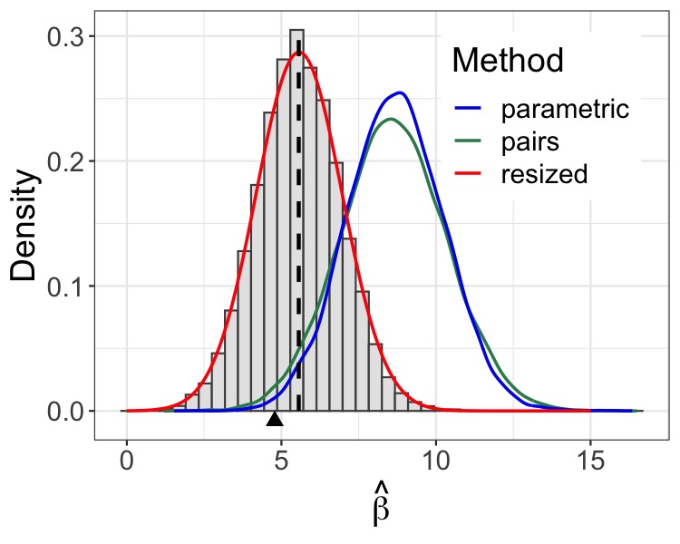
Figure 1: Histogram of the logistic MLE of a randomly chosen coefficient in 10,000 repeated experiments. Here, the covariates are sampled from a multivariate $t$-distribution with 8 degrees of freedom. The bootstrap MLE densities are displayed for the parametric bootstrap (blue), the pairs bootstrap (green) and the proposed resized bootstrap (red). The triangle indicates the true coefficient and the dashed line indicates the average MLE.

Next, we apply the parametric bootstrap and pairs bootstrap and display in Figure 1 the density curves of the bootstrap MLEs from one experiment.

• For the parametric bootstrap, we generate samples by fixing the covariates at the observed values and sample responses from a logistic model whose coefficients equal the MLE; put another way, we choose $\hat{F}={F}_{\hat{\beta}}$. The parametric bootstrap (blue) does not begin to describe the MLE distribution since the average value is 8.68, about twice that of the true coefficient, and the std. dev. is 1.55.

• The pairs bootstrap generates bootstrap samples by sampling with replacement from the observed data, i.e., we choose $\hat{F}$ to be the empirical distribution. The pairs bootstrap also fails to approximate the MLE distribution since the green curve shifts to the right and is much wider than the histogram (mean is 8.63 and std. dev. 1.71).

Finally, the red curve in Figure 1 shows the accuracy of the proposed resized bootstrap. We can see that this best describes the MLE distribution; for instance, both the mean (5.54) and standard deviation (1.39) are close to the true values.

2 Why does the bootstrap fail?

The pairs bootstrap fails in the high-dimensional setting because it effectively inflates the dimensionality ratio $\kappa=p/n$. In particular, when $n$ is large, the number of unique pairs $(X_{i}^{*},Y_{i}^{*})$ in a bootstrap sample is approximately $(1-1/e)n$ on average [30]. Consequently, the effective dimensionality ratio $\kappa e/(e-1)$ in the bootstrap sample is larger than $\kappa$. Because the bias and variance of the MLE increase as $\kappa$ increases [29, Figure 7], the pairs bootstrap tends to over-estimate both the bias and standard error.

While the pairs bootstrap over-estimates $\kappa$, the parametric bootstrap fails because the signal strength $\gamma$ is inflated in the bootstrap samples. Suppose for simplicity that the covariates are independent $\mathcal{N}(0,1)$. Then [29, Theorem 2] shows that

$$\lim_{n,p\to\infty}\operatorname{Var}({X}_{\text{new}}^{\top}\hat{{\beta}})\stackrel{{\scriptstyle a.s.}}{{=}}\alpha_{\star}^{2}\gamma^{2}+\kappa\sigma_{\star}^{2}>\gamma^{2},$$ (2)

whereas $\operatorname{Var}(X^{\top}\beta)=\gamma^{2}$. Here, $X_{\text{new}}$ is a new random sample independent from the training set. Because a higher $\gamma$ leads to higher bias and variance [29, Figure 7], the parametric bootstrap also tends to over-estimate the bias and standard error of the MLE.

In addition to over-estimating the bias and standard error, another problem of using the bootstrap is that when working with bootstrap samples, the MLE may cease to exist. We can explain this issue via the phase transition: for every ratio $\kappa$ and intercept $\beta_{0}$, there exists an asymptotic threshold $\gamma(\kappa,\beta_{0})$ such that the MLE does not exist once the signal strength $\gamma>\gamma(\kappa,\beta_{0})$. Similarly, for every $\gamma$ and $\beta_{0}$, there exists a threshold $\kappa(\gamma,\beta_{0})$ such that the MLE does not exist once $\kappa>\kappa(\gamma,\beta_{0})$. Because the pairs bootstrap over-estimates $\kappa$ while the parametric bootstrap over-estimates $\gamma$, the bootstrap MLE may not exist if either $\kappa$ or $\gamma$ exceeds the phase transition threshold. Figure 2 provides a visual illustration of these points.

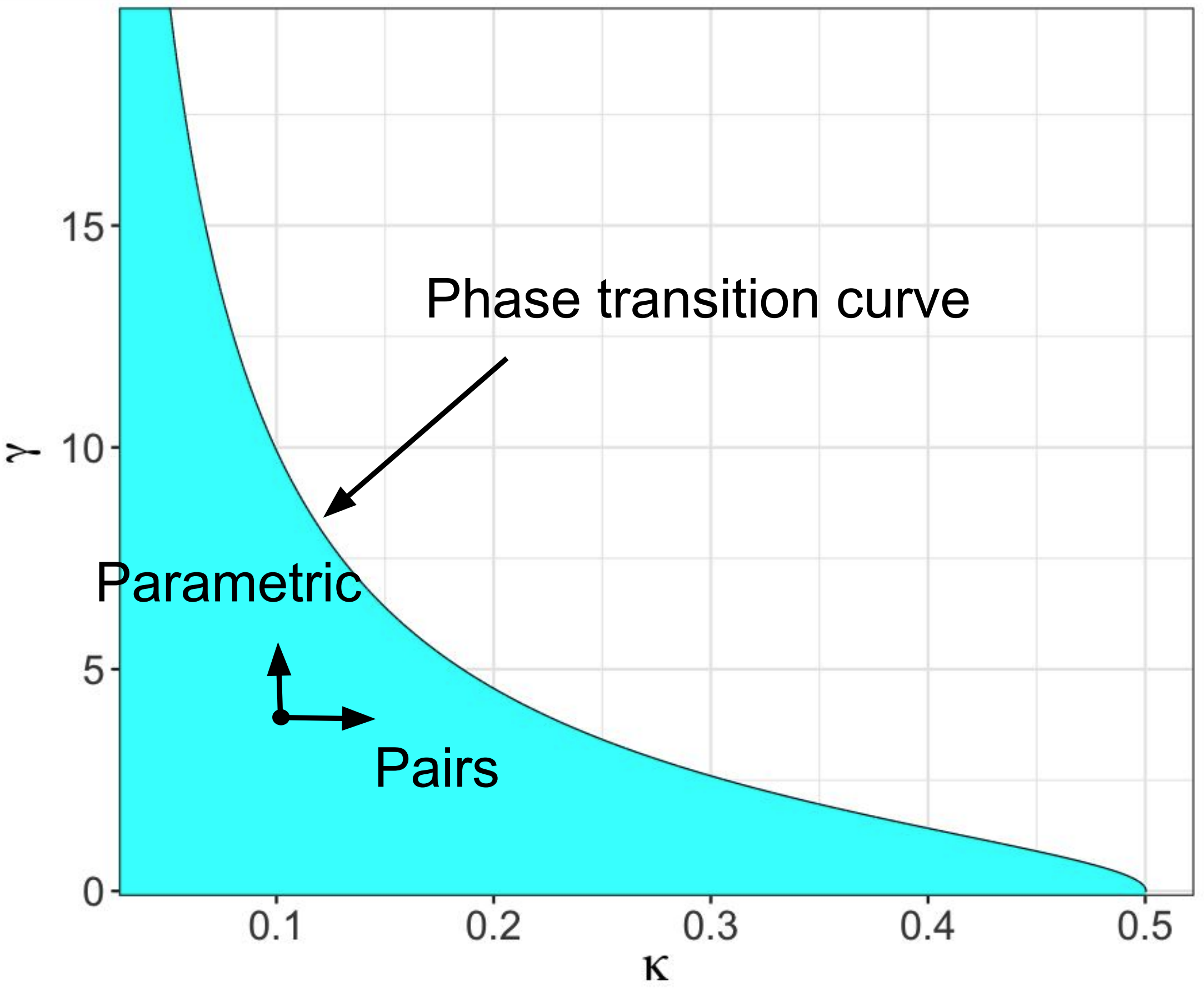
Figure 2: According to the high-dimensional theory (Section 1.1), the asymptotic distribution of the MLE depends on the problem dimension $\kappa$ and the signal strength $\gamma$. The pairs bootstrap over-estimates $\kappa$ whereas the parametric bootstrap over-estimates $\gamma$. Therefore, both methods lead to incorrect estimates of the MLE distribution. The blue region shows pairs of values of $(\kappa,\gamma)$ where the MLE exists.

3 A resized bootstrap

We proposing constructing parametric bootstrap samples from $F_{\beta_{\star}}$, where $\beta_{\star}$ is obtained by shrinking the MLE towards zero. We would like $\beta_{\star}$ to obey $\operatorname{Var}(X_{\text{new}}^{\top}\beta_{\star})=\gamma^{2}=\operatorname{Var}(X^{\top}\beta)$ as to preserve the signal-to-noise ratio. We set out to estimate $\gamma$ in Section 3.1 since $\gamma$ is unobserved. Upon obtaining $\beta_{\star}$, we follow the standard parametric bootstrap procedure to generate bootstrap samples. That is to say, the $b$th bootstrap sample consists of $({x}_{i},Y_{i}^{b})$, $i=1,\ldots,n$, where ${x}_{i}$ is the vector of features for the $i$th sample and $Y^{b}_{i}$ is sampled from our GLM with features $x_{i}$ and coefficients ${\beta}_{\star}$. We then compute the bootstrap MLE $\hat{{\beta}}^{b}\in\mathbb{R}^{p}$ by fitting the GLM using pairs $(x_{i},Y_{i}^{b})$. Repeating this process $B$ times yields $B$ bootstrap MLEs. We then infer the inflation and std. dev. of the MLE from the bootstrap MLE.

We summarize the procedure in Algorithm 2 and discuss how to compute confidence intervals using the bootstrap MLE in Section 3.2. We evaluate our method through simulated examples in Section 4.

3.1 Estimating the signal strength

Since we would like to have $\operatorname{Var}({X_{\text{new}}}^{\top}{\beta}_{\star})=\gamma^{2}$, we discuss how to estimate $\gamma$ from observed data (see Algorithm 1 for a summary). We begin by reviewing the existing ProbeFrontier method, which applies to Gaussian covariates, and then introduce a new approach applicable to general covariate distributions.

The ProbeFrontier method [29] estimates $\gamma$ by using the phase transition curve $\kappa(\beta_{0},\gamma)$: if the intercept equals $\beta_{0}$ and the signal strength equals $\gamma$, then the MLE does not exist almost surely (asymptotically) if $\kappa>\kappa(\beta_{0},\gamma)$; that is, the cases and controls can be perfectly separated by a hyperplane (see Section 2). The ProbeFrontier method identifies the threshold $\hat{\kappa}_{s}$ at which the MLE ceases to exist by subsampling observations. It then estimates $\hat{\gamma}$ in such a way that $\kappa(\beta_{0},\hat{\gamma})=\hat{\kappa}_{s}$ holds. While the ProbeFrontier method accurately estimates $\gamma$ when the covariates are Gaussian, it does not apply here because the phase transition curve actually depends on the covariate distribution. For example, if the covariates are from a multivariate $t$-distribution, then the phase transition curve depends on the degrees of freedom of the $t$-distribution [31].

As an alternative, we estimate $\gamma$ by using a one-to-one relation between

$$\gamma^{2}=\operatorname{Var}({X_{\text{new}}}^{\top}{\beta})\quad\text{and}\quad\eta^{2}=\operatorname{Var}({X_{\text{new}}}^{\top}\hat{\beta}).$$ (3)

The orange curve in Figure 3 plots $\eta$ as $\gamma$ varies, and we observe that $\eta(\gamma)$ increases monotonically when $\gamma$ increases. (Once again, this is because both the bias and the variance of the MLE increase as $\gamma$ increases [29, Figure 7].) Since the MLE does not exist when $\gamma$ exceeds the phase transition threshold, we expect that $\eta$ would increase to infinity as $\gamma$ approaches the threshold.

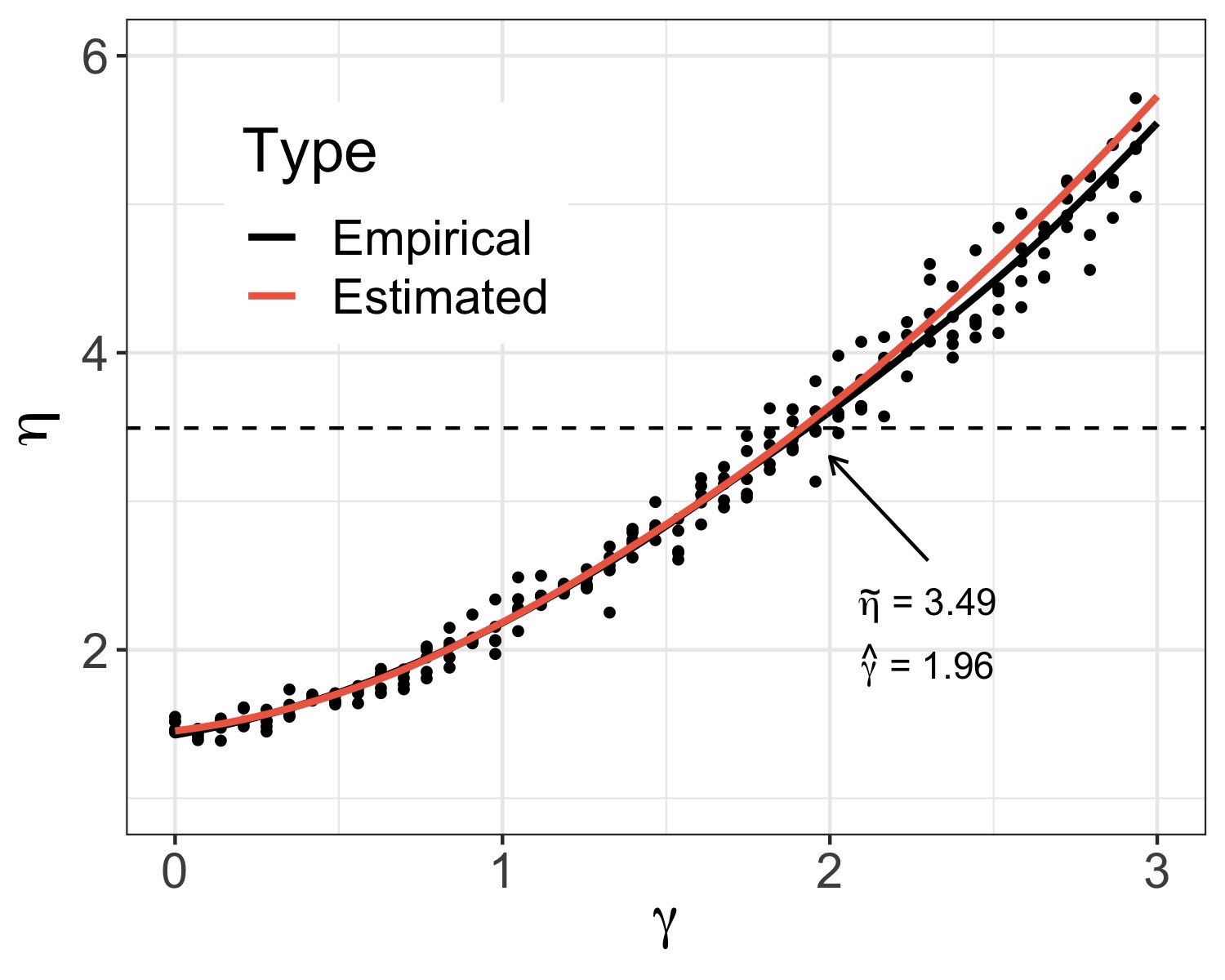
Figure 3: An illustration of using $\eta={\operatorname{sd}}({X_{\text{new}}}^{\top}\hat{\beta})$ to estimate the signal strength $\gamma={\operatorname{sd}}({X_{\text{new}}}^{\top}\beta)$. The orange curve shows $\eta$ versus $\gamma$. This is obtained by generating 100 random samples for each $\gamma$, the orange curve being the smoothed LOESS fit. The black curve shows an estimated curve using one dataset only; it is a smoothed version of $\hat{\eta}(\gamma)$ (black points). The dashed line shows $\tilde{\eta}$, and the estimated $\hat{\gamma}=1.96$ approximates $\gamma=2$ well. Here, we sample covariates from a multivariate $t$-distribution and responses from a logistic model. The coefficients ${\beta}$ are sampled once and then re-scaled to achieve a value of $\gamma$ shown on the $x$-axis.

The one-to-one relation between $\gamma$ and $\eta(\gamma)$ suggests that, if $\operatorname{Var}(X^{\top}\beta_{\star})\cong\operatorname{Var}(X^{\top}\beta)$, then $\operatorname{Var}(X^{\top}\hat{\beta}_{\star})\cong\operatorname{Var}(X^{\top}\hat{\beta})$, where $\hat{\beta}_{\star}$ denotes the MLE when the true coefficient is $\beta_{\star}$. Thus, we estimate $\gamma^{2}$ by $\operatorname{Var}(X^{\top}\beta_{\star})$, where $\beta_{\star}$ obeys

$$\operatorname{Var}({X_{\text{new}}}^{\top}\hat{\beta}_{\star})=\eta^{2}.$$ (4)

In this paper, we set $\beta_{\star}$ to be a rescaled version of the MLE, i.e., $\beta_{\star}=s\times\hat{\beta}$. Because the MLE is biased upwards in absolute magnitude, the rescaling factor $s$ is less than one and shrinks the MLE towards zero.

Although we cannot compute $\eta$ directly because it is evaluated at a new observation ${X_{\text{new}}}$, we estimate $\eta$ by using the SLOE estimator introduced in [32]. We briefly describe SLOE here, and defer detailed formulae to Appendix B. The SLOE estimator proceeds in two steps. First, it approximates $\operatorname{Var}({X_{\text{new}}}^{\top}\hat{\beta})$ by the variance of $x_{i}^{\top}\hat{\beta}_{(i)}$ where $\hat{\beta}_{(i)}$ is the leave-$i$th-observation-out MLE. Second, instead of re-evaluating $\hat{\beta}_{(i)}$ for each observation, SLOE uses the first-order approximation of the score equation to approximate $\hat{\beta}_{(i)}$ from the MLE. The theory is this: [32] proves that the SLOE estimator is consistent in logistic regression models with Gaussian covariates. Furthermore, we expect that SLOE yields reliable estimates for a broad class of covariates, for which the Euclidean norm $\|X\|$ is concentrated and the Hessian at the MLE is positive definite.

Now that we are able to approximate $\eta(\gamma)$ at a given $\gamma$, we estimate $\eta=\operatorname{Var}(X^{\top}\hat{\beta})^{1/2}$ and denote it as $\tilde{\eta}$. Next, we estimate the curve ${\eta}(t)$ at a sequence of signal strengths $t$, from which we estimate $\gamma$ by setting $\hat{\gamma}$ such that $\tilde{\eta}=\hat{\eta}(\hat{\gamma})$. To implement this, we pick a sequence of scaling factors $\{0=s_{1},\ldots,s_{I}=1\}$. At each $s_{i}$, we set the coefficients to be ${\beta}^{s_{i}}=s_{i}\times{\hat{\beta}}$ and the signal strength corresponding to $s_{i}$ as $\gamma(s_{i})=\operatorname{sd}(\boldsymbol{X}{\beta}^{s_{i}})$, where $\boldsymbol{X}$ refers to the observed covariate matrix. We use ${\beta}^{s_{i}}$ as the true coefficient to generate new responses (as in a parametric bootstrap) and then use this sample to obtain one estimate of $\hat{\eta}(\gamma(s_{i}))$. Repeating the process $J$ times yields $J$ estimates $\hat{\eta}_{j}(\gamma(s_{i}))$ for every $s_{i}$. We next fit a smoothed curve $\hat{\eta}(\gamma(s_{i}))$ through the points $\hat{\eta}_{j}(\gamma(s_{i}))$, $i=1,\ldots,I$, $j=1,\ldots,J$. Finally, we set $\hat{\gamma}$ such that $\hat{\eta}(\hat{\gamma})=\tilde{\eta}$.

We demonstrate our method in Figure 3, which shows $\hat{\eta}(\gamma(s_{i}))$ estimated from a single dataset. The estimated curve offers an excellent fit across all values of $\gamma$. In this example, the estimated $\tilde{\eta}=3.49$ (dashed horizontal line), and this corresponds to $\hat{\gamma}=1.96$ on the black curve. This estimate is close to the actual signal strength set to $\gamma=2$.

Input: Observed data $({x}_{i},y_{i})$, $1\leq i\leq n$, and a GLM formula.

1 Estimate $\tilde{\eta}=\operatorname{Var}(X^{\top}\hat{\beta})$ via leave-one-out techniques;

2 Pick a sequence $\{0=s_{1},\ldots,s_{I}=1\}$;

3 for $i=1,\ldots I$ do

4       Set ${\beta}^{s_{i}}=s_{i}\times\hat{\beta}$ and $\gamma_{i}=\mathrm{sd}(\boldsymbol{X}\beta^{s_{i}})$;

5       for $j=1,\ldots,J$ do

6             Simulate $Y_{i}^{j}$ given ${x}_{i}$ using ${\beta}^{s_{i}}$ as model coefficients;

7             Fit a GLM for $({x}_{i},Y_{i}^{j})$ to estimate $\hat{\eta}_{j}(\gamma(s_{i}))$;

8            

9       end for

10      

11 end for

12Fit a smooth curve $\hat{\eta}(\gamma)$;

13 Estimate $\hat{\gamma}$ by solving $\hat{\eta}(\hat{\gamma})=\tilde{\eta}$;

Output: Estimated $\hat{\gamma}$.

Algorithm 1 Estimating signal strength

3.2 Constructing confidence intervals

We consider two ways of computing confidence intervals (CI) from bootstrapped MLEs: first, assuming that the MLE is approximately Gaussian, i.e.,

$$\frac{\hat{\beta}_{j}-{\alpha}_{j}\beta_{j}}{\sigma_{j}}\approx\mathcal{N}(0,1),$$ (5)

where $\alpha_{j}$ and $\sigma_{j}$ denote the bias and standard deviation, inverting Eqn. (5) yields the following $(1-q)$ CI for $\beta_{j}$:

$$\left[\frac{1}{\hat{\alpha}_{j}}\left(\hat{\beta}_{j}-z_{1-q/2}\,\hat{\sigma}_{j}\right),\frac{1}{\hat{\alpha}_{j}}\left(\hat{\beta}_{j}-z_{q/2}\,\hat{\sigma}_{j}\right)\right].$$ (6)

Here, $z_{q}$ is the quantile of a standard Gaussian, while $\hat{\alpha}_{j}$ and $\hat{\sigma}_{j}$ refer to estimates of $\alpha_{j}$ and $\sigma_{j}$.

When the normal approximation is inadequate, we use the approximation

$$\frac{\hat{\beta}_{j}-{\alpha}_{j}\beta_{j}}{\sigma_{j}}\stackrel{{\scriptstyle d}}{{\approx}}\frac{\hat{\beta}^{b}_{j}-{\alpha}_{j}\beta_{\star,j}}{{\sigma}_{j}},$$ (7)

where the right-hand side refers to the distribution of $\hat{\beta}_{j}^{b}$ conditional on the observed covariates. After plugging in the estimated $\hat{\alpha}_{j}$ and $\hat{\sigma}_{j}$, we obtain a $(1-q)$ CI as

$$\left[\frac{1}{\hat{\alpha}_{j}}\left(\hat{\beta}_{j}-t_{j}^{b}[1-q/2]\,\hat{\sigma}_{j}\right),\frac{1}{\hat{\alpha}_{j}}\left(\hat{\beta}_{j}-t_{j}^{b}[q/2]\,\hat{\sigma}_{j}\right)\right],$$ (8)

where $t_{j}^{b}[q]$ denotes the quantile of the right-hand side of (7). We refer to the confidence interval in (8) as the “bootstrap-$t$” confidence interval, and examine the approximation (7) in Section 4.3.

Finally, we describe how to estimate the bias $\alpha_{j}$ and the standard deviation $\sigma_{j}$. To estimate $\sigma_{j}$, we use the standard deviation of the bootstrap MLE, i.e.,

$$\hat{\sigma}_{j}^{2}=\frac{1}{B-1}\sum_{b=1}^{B}(\hat{\beta}_{j}^{b}-\bar{\beta}_{j})^{2},\quad\text{where}\quad\bar{\beta}_{j}=\frac{1}{B}\sum_{b=1}^{B}\hat{\beta}_{j}^{b}.$$ (9)

We estimate $\alpha_{j}$ by weighted regression: that is, we regress $\bar{{\beta}}^{b}$ onto $\beta_{\star}$ by assigning to each MLE coordinate a weight inversely proportional to its estimated variance $\hat{\sigma}_{j}^{2}$. We assume a common bias factor because all the ${\alpha}_{j}$’s are equal when the covariates are multivariate Gaussian. In practice, we can plot $\bar{\beta}_{j}^{b}$ versus $\beta_{\star,j}$: if bias factors are all equal, then the points should align on a line, which we observe in all our simulations (Section 4).

Input: Observed data $({x}_{i},y_{i})$, $1\leq i\leq n$, and a GLM formula.

1 Compute resized coefficients ${\beta}_{\star}$;

2 for $b=1,\ldots,B$ do

3       Simulate $Y_{i}^{b}$ given ${x}_{i}$ using ${\beta}_{\star}$ as model coefficients;

4       Fit a GLM for $({x}_{i},Y_{i}^{b})$ to obtain the bootstrap MLE $\hat{{\beta}}^{b}$;

5      

6 end for

7Estimate the standard deviation of the MLE $\hat{\sigma}_{j}$ (See Eqn. (9));

8 Estimate a common factor $\hat{\alpha}$ by regressing $\bar{{\beta}}$ onto ${\beta}_{\star}$ with weights proportional to $1/\hat{\sigma}_{j}^{2}$;

Output: $\hat{\alpha}$ and $\hat{\sigma}_{j}$

Algorithm 2 Resized bootstrap procedure

3.3 When is the resized bootstrap adequate?

When the covariates are multivariate Gaussian, [28] observed that while Eqn. (1) is accurate when $\beta_{j}$ is moderately large, the std. dev. of $\hat{\beta}_{j}$ increases as the absolute magnitude of $\beta_{j}$ increases. This result implies that the resized coefficient $\beta_{\star,j}$ should be close to $\beta_{j}$ in order to correctly estimate the MLE distribution. However, the resized coefficients only satisfy $\operatorname{Var}(X^{\top}{\beta}_{\star})=\gamma^{2}$, and yet $\beta_{\star_{j}}\neq\beta_{j}$ in general. Therefore, we expect that the CIs to be approximately correct when $\beta_{j}$ is moderately large, but inaccurate when $\beta_{j}$ is large. We explore the performance of our method when the model coefficients are large in Appendix C. While we expect that correct inference can be obtained by shrinking the large and small coefficients separately, we leave this study for future research.

4 Numerical studies

We now study the accuracy of the proposed resized bootstrap method by simulating GLMs with non-Gaussian covariates. We consider logistic regressions in Section 4.2-4.3 and Poisson regression in Section 4.4. We report results of other examples in Appendix A.

4.1 Simulation design

First, we set $n=4000$ and $p=400$ ($\kappa=p/n=0.1$). Second, we consider two cases of covariate distributions:

1. The covariates follow a multivariate $t$-distribution (MVT) with $\nu=8$ degrees of freedom whose covariance matrix $\Sigma$ is a circulant matrix equal to $\Sigma_{ij}=0.5^{\min(|i-j|,p+1-|i-j|)}$. This structure implies that the variance of a predictor conditional on the others is the same regardless of the predictor. In turn, HDT then predicts that all the MLE coefficients have equal standard deviation.

2. The covariates follow a modified ARCH model ${X}=\zeta{\varepsilon}$, where $\zeta$ is the inverse of a $\chi$ variable with $\nu=8$ degrees of freedom and ${\varepsilon}$ is from an Autoregressive Conditional Heteroskedasticity (ARCH) model (see [33, Section 5.4] for a definition of ARCH models). Here, starting with $X_{0}\sim\mathcal{N}(0,\alpha_{0}/(1-\alpha_{1}))$, we sequentially sample variables so that $X_{j}=\sigma_{j}\varepsilon_{j}$, where $\sigma_{j}^{2}=\alpha_{0}+\alpha_{1}X_{j-1}^{2}$ and $\varepsilon_{j}\sim\mathcal{N}(0,1)$. We work with $\alpha_{0}=0.6$ and $\alpha_{1}=0.4$. Although uncorrelated, the covariates are not independent of each other.

After sampling the covariates, we sample responses from a logistic model. We sample model coefficients by first picking 50 non-null variables; then, we sample the magnitude of the non-null coefficients from an equal mixture of $\mathcal{N}(5,1)$ and $\mathcal{N}(-5,1)$. This signal strength ensures that the MLE exists. At the same time, the signal strength is strong enough such that we can tell a large proportion the the non-null variables apart from the nulls. For instance, when $\beta_{j}=4.78$ as in the example in Section 1.2 , over 90% of the 95% CI excludes 0, and approximately 90% of the non-null coefficients from the mixture distribution satisfy this property.

4.2 Results

We report below the estimated bias and standard deviation of the MLE as well as the coverage proportions. We also examine the MLE distribution and the assumption that the bias factors $\alpha_{j}$ are all equal. Without specifying, we consider covariates from a multivariate $t$-distribution.

4.2.1 Estimated Bias and Variance

From Section 1.1 we know that the MLE is just too sure in the sense that the estimated magnitude is biased upwards. As an illustration, Figure 4 plots the average MLE versus the model coefficients when the covariates are from (modified) ARCH model above. Since the scatterplot lies near a line, we can see that the $\alpha_{j}$’s do not seem to much depend on the magnitude of the coefficients; additionally, the plot confirms the bias of the MLE since the line has a slope greater than 1. For information, we get a very similar plot for the multivariate $t$-covariates.

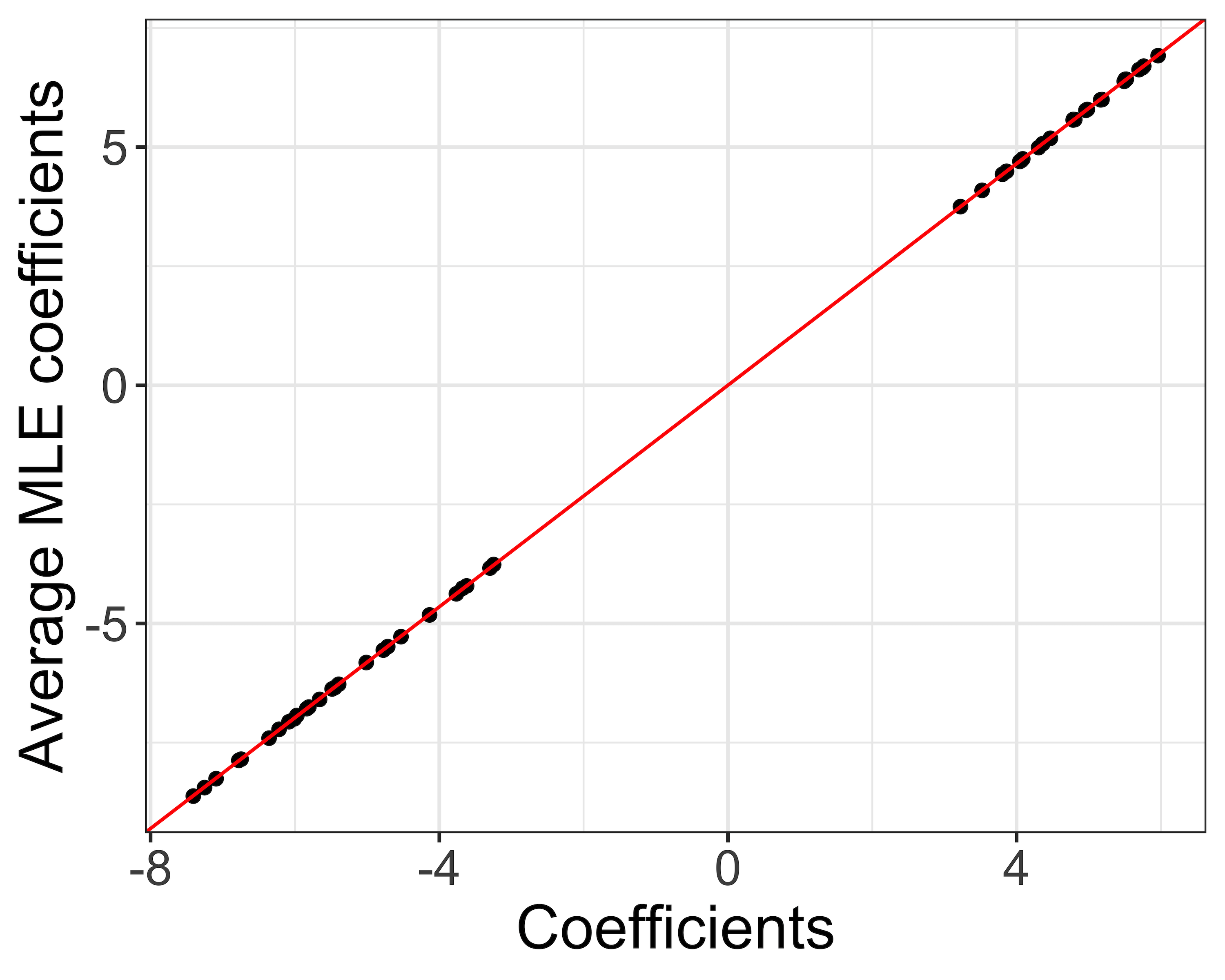
Figure 4: Average MLE versus model coefficients for the non-null variables. The $x$-axis shows the magnitude of each non-null coefficient and the $y$-axis shows the average MLE over 10,000 repetitions. The red line has zero intercept and slope equal to 1.16.

We now examine the accuracy of the estimated bias using existing high-dimensional theory and the resized bootstrap (recall that both estimate a common bias factor). Table 1 reports the estimated bias and variance of a single null and a single non-null variable. As observed in Section 1.2, HDT captures the bias, and Table 1 shows that the resized bootstrap estimate is also reasonably accurate. As to the standard deviation, while both methods slightly underestimate the std. dev., the resized bootstrap is more accurate and its relative error is less than 3%. In particular, the resized bootstrap captures the increased std. dev. of the MLE of non-null variables in comparison to null variables. In contrast, classical calculations based on the Fisher information significantly underestimate the std. dev.. Since the resized bootstrap yields a more accurate std. dev., we would expect enhanced CIs.

	Bias			Standard Deviation
	High-dim	Resized	Empirical	Classical	High-dim	Resized	Empirical
	Theory	Bootstrap	Bias	Theory	Theory	Bootstrap	Std. dev.
$\beta=0$	-	-	-	1.232	1.259	1.316	1.327
$\beta=5.519$	1.151	1.159	1.160	1.244	1.259	1.327	1.337

Table 1: Estimated bias and std. dev. of the MLE. The correct values (empirical bias and std. dev.) have been obtained from 10,000 repetitions. The std. dev. from classical theory is calculated by the glm function in R and averaged over 10,000 repetitions. The resized bootstrap estimates are computed by taking an average over 1000 repetitions and uses an estimated signal strength $\gamma$.

4.2.2 Coverage Proportion

Section 3.2 introduced two types of CIs, based on the assumptions that the MLE is approximately Gaussian (Eqn. (5)) or that the standardized bootstrap MLE approximates the distribution of the standardized MLE (Eqn. (7)). Before evaluating accuracy, we examine these assumptions by showing a normal Q-Q plot of the MLE (Figure 5, Left) and a Q-Q plot of the standardized bootstrap MLE versus the standardized MLE (Figure 5, Right). Here, we standardize the bootstrap MLE by the estimated bias and estimated std. dev. and the MLE by the correct bias and std. dev.. Along the points align on the 45 degree line in both plots, we conclude that both assumptions are reasonable and, therefore, expect that both CIs would perform well.

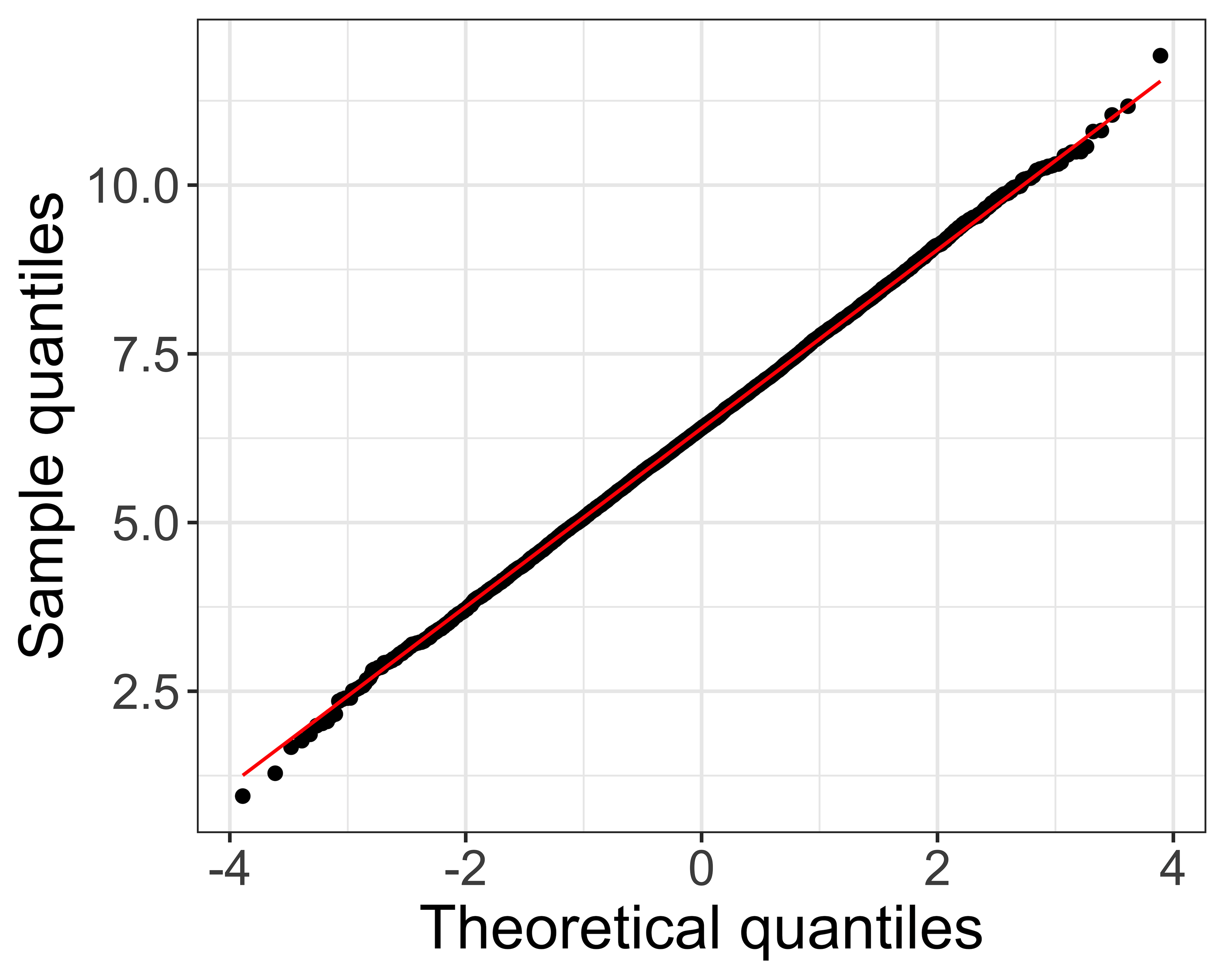
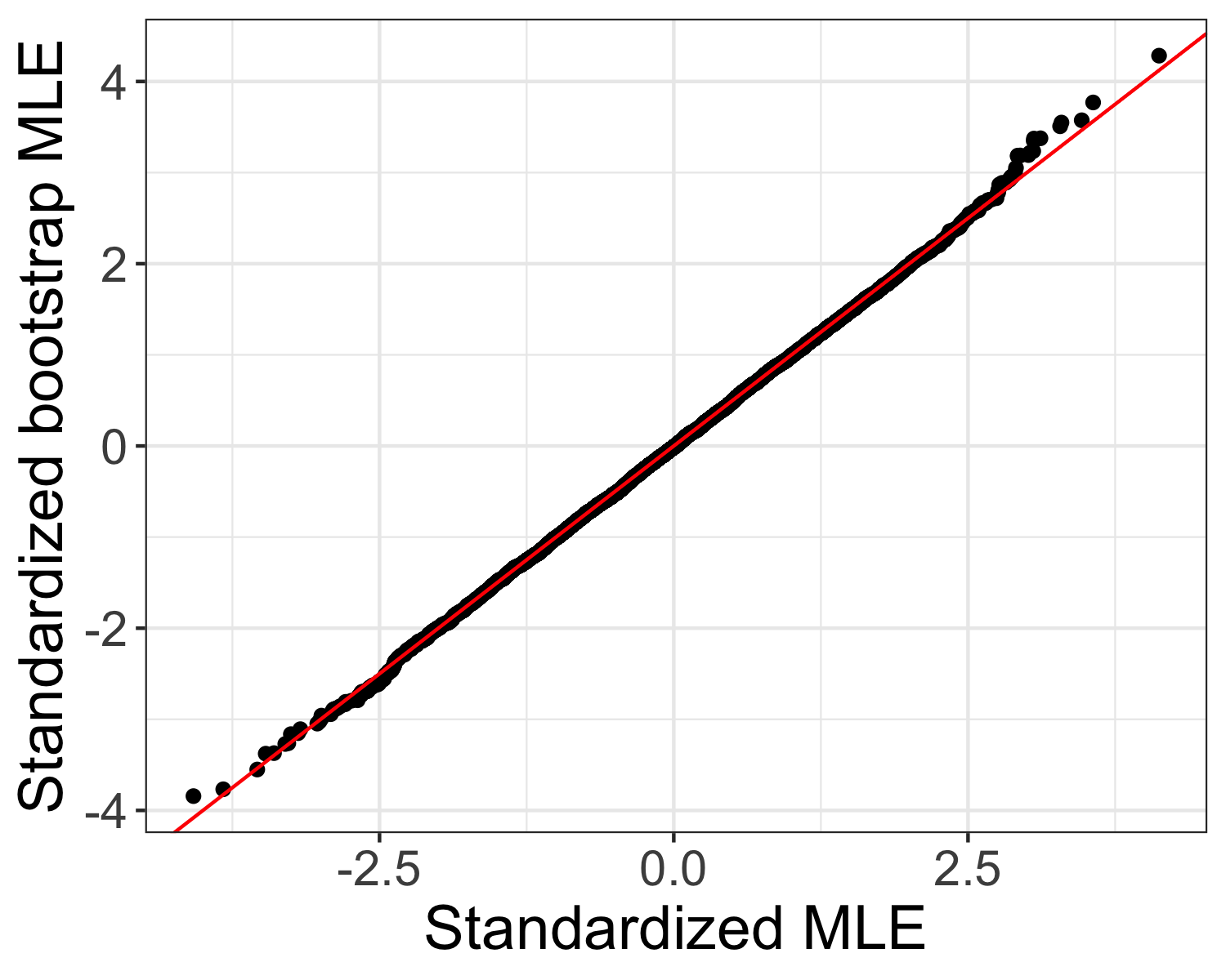
Figure 5: (Left) Normal Q-Q plot of the MLE. (Right) Q-Q plot of the standardized bootstrap MLE (in one simulated example) versus the standardized MLE. In this example, the covariates are sampled from a multivariate $t$-distribution.

Denote the confidence interval for $\beta_{j}$ in the $i$th simulation as $\operatorname{CI}_{i,j}$, and define the proportion of times a single variable $\beta_{j}$ is covered (Table 2) as

$$q_{j}:=\frac{1}{N}\sum_{i=1}^{N}\operatorname{\mathbb{I}}\{\beta_{j}\in\operatorname{CI}_{i,j}\}.$$ (10)

Define the coverage proportion of all of the variables in the $i$th experiment only (Table 3) as

$$\bar{q}_{i}=\frac{1}{p}\sum_{j=1}^{p}\operatorname{\mathbb{I}}\{\beta_{j}\in\operatorname{CI}_{i,j}\}$$ (11)

We report both coverage of a single coefficient $q_{j}$ and the proportion of variables covered in a single-shot experiment $\bar{q}=\frac{1}{N}\sum_{i=1}^{N}\bar{q}_{i}$ in Tables 2 and 3. Both the Gaussian approximation (Boot-$g$) and bootstrap MLE distribution (Boot-$t$) are used to compute the CIs. The two CIs not only differ in their formulae, but also in the number of bootstrap samples: we use $B=10,000$ bootstrap samples to compute the boot-$t$ CI, but only $B=100$ bootstrap samples to compute the boot-$g$ CI. This is because boot-$g$ CI requires only estimates of the bias and variance, while boot-$t$ CI requires an estimate of the entire distribution.

	Theoretical CI		Standard Bootstrap		Resized Bootstrap
Nominal					Known $\gamma$		Estimated $\gamma$
coverage	Classical	High-Dim	Parametric	Pairs	Boot-$g$	Boot-$t$	Boot-$g$	Boot-$t$
95	87.3	93.5	71.1	76.3	93.6	93.9	94.2	94.4
	(0.3)	(0.3)	(1.6)	(1.3)	(0.7)	(0.7)	(0.8)	(0.8)
90	79.4	87.9	61.2	66.6	88.5	88.7	88.6	89.1
	(0.30)	(0.3)	(1.7)	(1.4)	(1.0)	(1.0)	(1.1)	(1.1)
80	67.4	77.2	46.8	52.7	79.5	79.6	80.8	80.0
	(0.5)	(0.4)	(1.7)	(1.5)	(1.2)	(1.2)	(1.3)	(1.4)

Table 2: Coverage proportion of a single variable ($q_{j}$ in Eqn. (10)) with standard deviation between parentheses. This example uses multivariate-$t$ covariates.

	Theoretical CI		Standard Bootstrap		Resized Bootstrap
Nominal					Known $\gamma$		Estimated $\gamma$
coverage	Classical	High-Dim	Parametric	Pairs	Boot-$g$	Boot-$t$	Boot-$g$	Boot-$t$
95	92.5	93.7	90.8	93.3	94.6	94.9	94.7	95.0
	(0.02)	(0.02)	(0.06)	(0.05)	(0.04)	(0.04)	(0.04)	(0.04)
90	86.6	88.2	84.5	87.8	89.5	89.7	89.7	89.9
	(0.02)	(0.02)	(0.08)	(0.06)	(0.06)	(0.06)	(0.06)	(0.06)
80	75.7	77.7	73.6	77.5	79.4	79.5	79.6	79.7
	(0.03)	(0.03)	(0.09)	(0.08)	(0.08)	(0.08)	(0.08)	(0.08)

Table 3: The proportion of covered variables in a single-shot experiment ($\bar{q}$ in Eqn. (11)). The standard deviation is given between parentheses.

While the resized bootstrap slightly undercovers a single coefficient (Table 2), the relative error is within 1.5% in all of the levels we examined. Similarly, the proportion of variables covered in a single-shot experiment (Table 3) is also close to the nominal coverage and the relative error is within 1%. In addition, boot-$g$ and boot-$t$ CI achieve similar accuracy at every level we examined. Since boot-$g$ CI uses a smaller sample size, we prefer boot-$g$ CI when the Gaussian assumption holds. We can verify the normality assumption by comparing the quantiles of bootstrap MLEs with normal quantiles. Table 2 shows the coverage of a non-null variable, and we report coverage of a null variable in Appendix A.1. Comparing the coverage probability using the estimated signal strength $\hat{\gamma}$ versus its true value $\gamma$ shows that the method with estimated parameters perform as well as if we had an oracle.

As to the other methods, the HDT CIs slightly undercover since variability is underestimated as seen earlier. Classical CIs significantly undercover. Neither the parametric nor the pairs bootstrap provide the correct coverage, and this is consistent with observations from Figure 1.

4.3 Small sample sizes

We study an example with a small sample size, and set $n=400$ and $p=40$. We sample covariates independently from a Pareto distribution and sample responses from a logistic model where half of the variables are non-nulls and sampled from an equal mixture of $\mathcal{N}(5,1)$ and $\mathcal{N}(-5,1)$.

When the covariates are i. i. d., the MLE may be asymptotically Gaussian, however, the normal approximation is inaccurate when $n$ is small. To see this, we can express $\hat{\beta}_{j}$ as

$$\hat{\beta}_{j}=\frac{\lambda}{\kappa\sqrt{n}}\sum_{i=1}^{n}x_{ij}(y_{i}-\rho^{\prime}(x_{i,-j}^{\top}\hat{\beta}_{[-j]}))+o_{P}(1),$$ (12)

where $\hat{\beta}_{[-j]}$ refers to MLE computed when leaving out the $j$th variable and $\rho(t)=\log(1+e^{t})$ [29, Appendix C]. Although Eqn. (12) assumes that the $X_{ij}$ are standard Gaussian, we expect that it holds for other i. i. d. covariates. Since $\hat{\beta}_{j}$ is approximately a weighted average of the observed $x_{i,j}$, $\hat{\beta}_{j}$ approaches a Gaussian random variable as $n\to\infty$ by the central limit theorem. Since the rate of convergence depends on the third moment of $X_{ij}$ as a result of the Berry-Esseen theorem, we expect that the distribution of the MLE deviates from a Gaussian distribution when $n$ is small. Indeed, the normal quantile plot of $\hat{\beta}_{j}$ (Figure 6, Left) confirms that the MLE is skewed to the left and thus not Gaussian. In comparison, the normal quantile plot when $n=4000$ and $p=400$ (see Figure 9 in Appendix A.2) indicates that the MLE is well-approximated by a Gaussian distribution when $n$ is large.

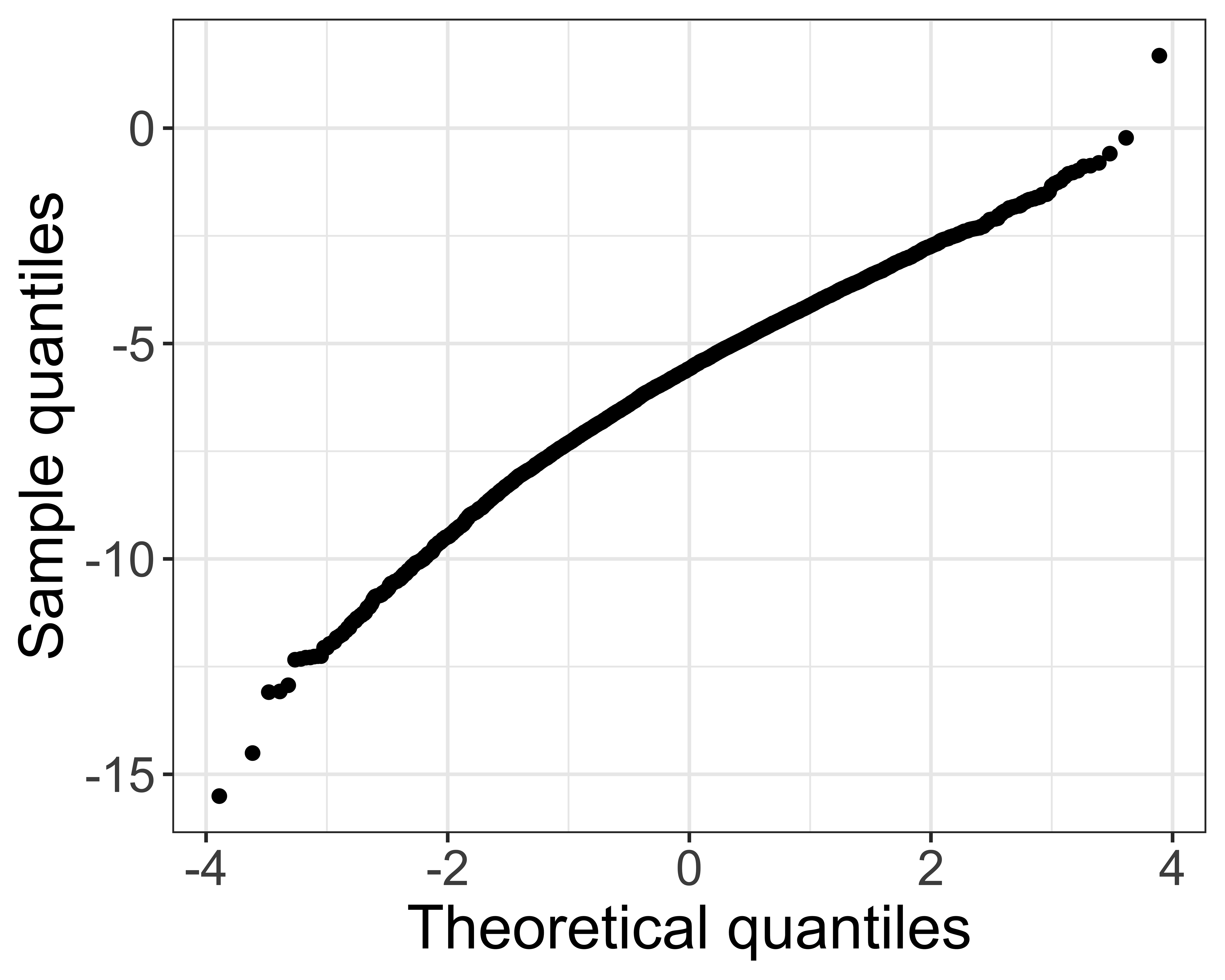
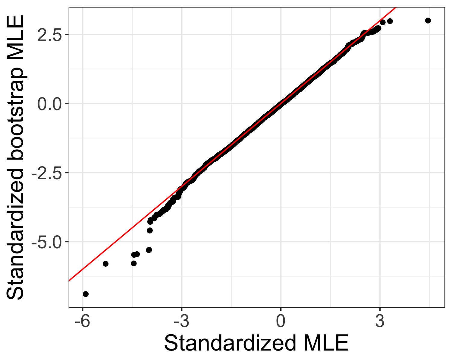
Figure 6: (Left) Normal quantile plot of a single MLE coordinate where $\beta=-4.6$ and $n=400$, $p=40$ and the covariates are i. i. d. from a Pareto distribution. (Right) Q-Q plot of the standardized MLE versus the bootstrap MLE in a single experiment. The standardization is as in Figure 5. The red line is the 45 degree line.

While the MLE is not Gaussian, a Q-Q plot of the standardized $\hat{\beta}_{j}^{b}$ versus the standardized $\hat{\beta}_{j}$ shows that the bootstrap MLE approximates the sampling distribution very well (Figure 6, Right). We thus expect that the resized bootstrap provides coverage. This is confirmed in Table 4, which shows that the bootstrap CIs are reasonably accurate for both a single variable and a single-shot experiment across all of the confidence levels examined. As before, the resized bootstrap using estimated parameters performs equally well as when we know the true values. While we do not report the coverage proportion using bootstrap-$g$ CIs, we observe that they yield similar accuracy as bootstrap-$t$ CI intervals. Lastly, we note that the bootstrap MLE (standardized by estimated bias and variance) has a lighter tail than the standardized MLE (standardized by the true bias and variance). This explains why the resized bootstrap CI slightly undercovers.

Our results in this example suggest that the bootstrap CIs produce reasonable coverage when the sample size is small and the normal approximation is far from valid. This in contrast to methods based on high-dimensional theory since we can see that the corresponding CI’s undercover. Again, this happens because variability is underestimated.

	I. Single variable			II. Single Experiment
Nominal	High-dim	Resized Bootstrap		High-dim	Resized Bootstrap
Coverage	Theory	Known-$\gamma$	Estimated-$\gamma$	Theory	Known-$\gamma$	Estimated-$\gamma$
95	88.7 (0.3)	95.2 (0.7)	95.7 (0.6)	91.6 (0.1)	94.8 (0.2)	95.6 (0.1)
90	81.6 (0.4)	90.0 (1.0)	91.5 (0.9)	86.0 (0.1)	89.7 (0.2)	90.9 (0.2)
80	70.0 (0.5)	78.6 (1.3)	81.0 (1.2)	75.7 (0.1)	79.2 (0.3)	80.4 (0.2)

Table 4: Coverage proportion of a single variable (Column I) and of all of the variables (Column II) in 10,000 repeated experiments with $n=400$ and $p=40$. We use the resized bootstrap method with known or estimated parameters. The standard deviations are reported between parentheses.

4.4 A Poisson regression example

We now consider an example with Poisson regression with log link function, i. e., $Y\,|\,X\sim\mathrm{Poisson}(\mu(X))$ and $\log(\mu(X))=X^{\top}\beta$ [34, Chapter 12]. We use the same simulation design as in Section 4.1, with the exception that the non-null coefficients are sampled from an equal mixture of $\mathcal{N}(3,1)$ and $\mathcal{N}(-3,1)$ to prevent $\mu(X)$ from being too large. We report the bias and std. dev. of both a null and a non-null variable in Table 5. We only use the classical theory and the resized bootstrap to estimate the std. dev., since HDT is unavailable for Poisson regression. Table 5 shows that the MLE is approximately unbiased and the std. dev. using the classical theory is quite accurate. The resized bootstrap also accurately estimates the std. dev. of the MLE. Therefore, we expect that both approaches would produce CI with correct coverage. Indeed, the coverage proportion using both the classical theory and the resized bootstrap method are quite accurate, as the average coverage proportions are within two standard deviations away from the nominal coverage (see Table 6). In sum, both the classical theory and the resized bootstrap yield reasonably accurate CI in case of a Poisson regression.

	Bias			Standard Deviation
	Resized Bootstrap		Empirical	Classical	Resized Bootstrap		Empirical
	Known-$\gamma$	Estimated-$\gamma$	Bias	Theory	Known-$\gamma$	Estimated-$\gamma$	Std. dev.
$\beta=0$	-	-	-	0.272	0.27	0.27	0.268
$\beta=3.24$	0.989	0.990	0.990	0.270	0.27	0.27	0.272

Table 5: Estimated bias and std. dev. of the MLE from a Poisson regression. Please see Table 1 for detailed description of the table.

	Nominal	Classical	Resized Bootstrap
	Coverage	Theory	Known-$\gamma$	Estimated-$\gamma$
Single Null	95	95.4 (0.2)	93.8 (0.7)	93.6 (0.7)
	90	90.4 (0.3)	89.1 (0.9)	89.3 (0.9)
	80	80.1 (0.4)	80.7 (1.1)	80.2 (1.2)
Single Non-null	95	94.6 (0.2)	95.1 (0.6)	94.3 (0.7)
	90	89.7 (0.3)	90.5 (0.8)	90.0 (0.9)
	80	79.2 (0.4)	80.0 (1.2)	80.1 (1.17)
Single Experiment	95	95.1 (0.01)	94.7 (0.04)	94.6 (0.04)
	90	90.2 (0.01)	89.6 (0.05)	89.6 (0.05)
	80	80.3 (0.02)	79.7 (0.06)	79.7 (0.07)

Table 6: Coverage proportion of a single null or non-null variable ($q_{j}$ in Eqn. (10)) and the proportion of covered variables in a single-shot experiment ($\bar{q}_{i}$ in Eqn. (11)). The coverage proportion is computed using 10,000 repetitions, and 1,000 for the resized bootstrap. We use boot-$g$ CI for the resized bootstrap. The standard deviations are reported between parentheses.

5 Application to a real data set

Having observed that the resized bootstrap procedure provides more accurate inference compared to classical and high-dimensional theory, we now analyze a real data set. In this study [35], researchers aim to understand which factors are associated with restrictive spirometry pattern (RSP), which is a lung condition. In particular, they hypothesize that glomerular hyperfiltration (GHF), which assesses the kidney function, may be associated with the risk of RSP. To evaluate their hypothesis, they collected participants data from from the Korea National Health and Nutrition Examination Survey (KNHANES) from 2009-2015. They performed a logistic regression, where the response variable is RSP (defined as FVC $<$ 80% AND FEV1/FVC $\geq$ 0.7) and the covariates include demographic variables, medical history, medications used, and a variety of health-related variables.

For the purpose of illustrating our approach, we fit a logistic regression using subsamples of sample size $n=200$ and include $p=18$ covariates including the intercept ($\kappa=18/200=0.09$). We examine whether the confidence intervals of the model coefficients, i.e. , the log odds ratios, cover the “true” coefficients, which we estimate by the logistic MLE using the full data that contains about 22,000 observations. Figure 7 shows the CI for each covariate using classical theory (black), resized bootstrap (red), and the estimated coefficient using the full data (black points). The resized bootstrap CI is closer to zero compared to CI using the classical theory, and is slightly more accurate. For instance, the coefficient for waist circumference is covered by the red segment, but is not covered by the black segment.

Figure 7: Confidence interval for each variable using classical theory (black) and the resized bootstrap (red). The black points indicate true model coefficients, estimated using the full data set. While we include demographic variables in the logistic model, we do not present their fitted coefficients as in Table 2 of the paper.

Then, we generate $B=25$ disjoint subsamples of sample size $n=180$ and compare classical theory and the resized bootstrap based on the estimated bias, std. dev., and the coverage proportion of CIs. First, we examine the bias of the MLE by plotting the average of the logistic MLE estimated using each subsample versus the true coefficients (Figure 8, Left). While the average MLEs are scattered across, their absolute magnitude is slightly larger than the true coefficients. The resized bootstrap yields an estimate $\hat{\alpha}_{b}=1.13$ (red). Though this is a small adjustment, it allows the resized bootstrap to produce more accurate CI as observed in Figure 7.

Next, we plot the average estimated std. dev. versus the empirical std. dev. in Figure 8 (Right) calculated across batches. The resized bootstrap and the classical estimates are similar, and both methods tend to underestimate the true standard deviation. In Table 7, we evaluate the proportion of variables covered in each batch as well as the coverage probability of the variable “systolic blood pressure”. Since both methods under-estimates the std. dev., we expect that the bootstrap provides some improvement in coverage, but does not yield correct coverage either, and this is indeed what we observe in the table. In this example, we use the large sample coefficient as a proxy for the true model coefficients, and our results suggest that when the sample size is small, while the resized bootstrap may not yield accurate coverage, it may perform better than the classical theory.

Figure 8: Bias and std. dev. of the MLE. (Left) Average MLE for the variables versus true coefficients. The black points show the average MLE averaged over $B=25$ batches. The red line shows the resized bootstrap estimate of the bias factor ($\hat{\alpha}_{b}=1.13$). (Right) Average estimated standard deviation of the MLE for each variable versus standard deviation across batches. The black and red points respectively use classical theory and the resized bootstrap. In both plots, the black line is the 45 degree line.

Nominal	I. Single variable		II. Single experiment
Coverage	Classical	Resized Bootstrap	Classical	Resized Bootstrap
95	87.5 (6.9)	91.3 (6.0)	92.2 (1.3)	95.0 (1.2)
90	87.5 (6.9)	87.0 (7.2)	85.8 (1.6)	88.2 (1.4)
80	83.3 (7.8)	82.6 (8.1)	72.3 (1.9)	74.7 (1.7)

Table 7: Coverage probability of confidence intervals (the coverage standard deviation is between parentheses). The first columns report the coverage proportion for the variable “systolic blood pressure”. The next two columns compute the proportion of variables covered in each batch and report the average over 25 batches.

6 Discussion

In this paper, we demonstrated that the distribution of the MLE in large logistic regression models depends on the distribution of the covariates and that bootrstrap methods fail to approximate this distribution. This is in line with previous findings concerned with linear regression [18, 19]. To fix this problem, we introduced a resized bootstrap, which correctly adjusts inference. The key is to resample from a parametric distribution obtained by shrinking the MLE towards zero in a data-dependent fashion, where the amount of shrinkage is informed by insights from HDT. Resized bootstrap CIs yield correct coverage proportions for different types of covariate distributions and types of GLMs. Our findings echo previous results in [19, 36]; combining HDT with bootstrap resampling methods can provide improved estimates.

We conclude with several future research questions. First, while the resized bootstrap procedure provides a high-quality approximation to the MLE distribution, it slightly underestimates the standard deviation. Therefore, future research on the theoretical accuracy of the procedure might lead to improvements in the design of the resized MLE, for example, by adjusting the coefficients to not only match the standard deviation of the linear predictor, but also a few higher moments. Second, one drawback of the resized bootstrap is its relatively high computational cost: we need to compute the MLE many times to estimate $\gamma$ and the MLE distribution. Although a few hundred bootstrap samples suffice to yield accurate CIs when the MLE is approximately Gaussian, being able to reduce the computational cost would make it even more suitable for larger datasets. Third, as mentioned in Section 3.3, the resized bootstrap is expected to accurately estimate the distribution of the MLE for coefficients with moderate magnitudes. While the resized bootstrap is reasonably accurate for relatively large $\beta_{j}$ (Appendix C), novel insights might further enhance it.

Acknowledgements

E. C. was supported by the Office of Naval Research grant N00014-20-1-2157, the National Science Foundation grant DMS-2032014, the Simons Foundation under award 814641, and the ARO grant 2003514594.

Appendix A Additional Simulation Results

This section provides additional simulation results to supplement the findings from Section 4.2.

Appendix A.1 reports the coverage proportion of null variables when covariates are from a multivariate $t$-distribution. Appendix A.3 shows the coverage proportion when covariates are from a modified ARCH model and the responses from a logistic and a probit model. Appendix A.2 shows the normal quantile plot of the MLE when the sample size is large and covariates are i. i. d.  from a Pareto distribution.

A.1 Coverage of a null variable

Table 8 reports the coverage proportion of a null variable when the covariates follow a multivariate $t$-distribution (see Section 4.1 for the simulation design). Coverage using either classical calculations or the standard bootstrap is better than for a non null, compare with Table 2. This is because we observed that the MLE is unbiased when $\beta_{j}=0$.

	Theoretical CI		Standard Bootstrap		Resized Bootstrap
Nominal					Known $\gamma$		Estimated $\gamma$
coverage	Classical	High-Dim	Parametric	Pairs	Boot-$g$	Boot-$t$	Boot-$g$	Boot-$t$
95	93.1	93.6	93.4	95.1	95.5	95.0	95.6	95.1
	(0.3)	(0.2)	(0.9)	(0.7)	(0.6)	(0.7)	(0.7)	(0.7)
90	87.4	88.1	88.7	91.2	90.0	90.2	89.7	90.1
	(0.3)	(0.3)	(1.1)	(0.9)	(0.9)	(0.9)	(1.0)	(1.0)
80	76.7	77.9	78.0	82.7	78.7	79.4	80.4	80.4
	(0.4)	(0.4)	(1.4)	(1.1)	(1.2)	(1.2)	(1.4)	(1.4)

Table 8: Coverage proportion of a single null variable ($q_{j}$ in Eqn. (10)) with standard deviation between parentheses. This example uses multivariate-$t$ covariates.

A.2 Normal Quantile Plot in Section 4.3

We are in the setting of Section  4.3, except that $n=4,000$ and $p=400$. We see from Figure 9 that the MLE is very well approximated by a Gaussian distribution. In contrast to the case of small samples where the MLE has a heavy left tail (Figure 6), we can say that the central limit theorem has kicked in.

Figure 9: Normal quantile plot of an non-null MLE coordinate. The covariates are i. i. d. from a Pareto distribution. Here, $n=4000$ and $p=400$.

A.3 Other Covariates and GLM

We now apply the resized bootstrap to construct CIs for model coefficients in logistic and probit regression models. The covariates follow our modified ARCH model. In all cases, we set $n=4000$, and $p=400$. In probit regressions, we sample model coefficients by first picking 50 non-null variables, and sample the corressponding coefficients to be from an equal mixture of $\mathcal{N}(3,1)$ and $\mathcal{N}(-3,1)$. High-dimensional theory is available for both logistic and probit regressions (the theory for probit is however unpublished).

		Theoretical CI		Resized Bootstrap
	Nominal			Known $\gamma$		Estimated $\gamma$
	coverage	Classical	High-Dim	Boot-$g$	Boot-$t$	Boot-$g$	Boot-$t$
Single Null	95	93.4	93.8	94.7	94.9	95.0	95.3
		(0.25)	(0.24)	(0.81)	(0.70)	(0.75)	(0.73)
	90	87.6	88.3	87.8	88.2	89.2	88.8
		(0.33)	(0.32)	(1.0)	(1.0)	(1.1)	(1.1)
	80	76.6	77.2	77.5	77.5	78.0	78.3
		(0.4)	(0.4)	(1.3)	(1.3)	(1.4)	(1.4)
Single Non-null	95	81.7	93.0	93.6	93.7	93.5	93.5
		(0.4)	(0.5)	(0.8)	(0.8)	(0.9)	(0.9)
	90	72.5	86.8	87.9	88.4	87.3	88.5
		(0.5)	(0.3)	(1.0)	(1.0)	(1.1)	(1.1)
	80	58.6	76.2	77.1	77.2	77.1	77.1
		(0.5)	(0.4)	(1.3)	(1.3)	(1.4)	(1.5)
Single Experiment	95	92.1	93.7	94.5	94.8	94.7	94.9
		(0.02)	(0.01)	(0.04)	(0.04)	(0.04)	(0.04)
	90	86.0	88.1	89.4	89.7	89.6	89.9
		(0.02)	(0.02)	(0.06)	(0.06)	(0.05)	(0.06)
	80	75.0	77.6	79.5	79.7	79.7	79.8
		(0.03)	(0.03)	(0.08)	(0.08)	(0.08)	(0.08)

Table 9: Coverage proportion of a single null variable, single non-null variable, and in a single-shot experiment with standard deviation between the parentheses. This example uses modified ARCH covariates and a logistic model. Here, we use both Gaussian approximation (Column Boog-$g$) and distribution of the bootstrap MLE (Column Boot-$t$) to construct the CI.

		Theoretical CI		Resized bootstrap
	Nominal			Known $\gamma$		Estimated $\gamma$
	coverage	Classical	High-Dim	Boot-$g$	Boot-$t$	Boot-$g$	Boot-$t$
Single Null	95	93.4	94.1	94.0	93.6	93.9	93.7
		(0.3)	(0.2)	(0.7)	(0.7)	(0.7)	(0.8)
	90	87.5	88.5	89.3	89.2	88.2	88.7
		(0.3)	(0.3)	(1.0)	(1.0)	(1.0)	(1.0)
	80	76.9	78.0	79.2	79.2	79.1	79.4
		(0.4)	(0.4)	(1.2)	(1.3)	(1.3)	(1.2)
Single Non-null	95	87.8	93.4	95.0	94.9	94.3	94.9
		(0.3)	(0.3)	(0.7)	(0.7)	(0.7)	(0.7)
	90	80.5	87.6	90.5	90.7	90.7	90.7
		(0.4)	(0.3)	(0.9)	(0.9)	(0.9)	(0.9)
	80	68.2	77.0	80.8	80.8	80.4	80.5
		(0.5)	(0.4)	(1.2)	(1.2)	(1.2)	(1.2)
Single Experiment	95	92.0	93.6	94.6	94.9	94.8	95.0
		(0.02)	(0.02)	(0.04)	(0.04)	(0.04)	(0.04)
	90	85.6	88.0	89.6	89.8	89.7	89.9
		(0.02)	(0.02)	(0.06)	(0.06)	(0.05)	(0.05)
	80	74.9	77.5	79.5	79.7	79.7	79.8
		(0.03)	(0.03)	(0.08)	(0.08)	(0.07)	(0.07)

Table 10: Coverage proportion of a single null variable, single non-null variable, and in a single-shot experiment with standard deviation between the parentheses. This example uses modified ARCH covariates and a probit model.

Appendix B The SLOE estimator

The Signal Strentgh Leave-One-Out Estimator (SLOE) provides an analytic expression for estimating $\eta^{2}=\lim_{n\to\infty}\operatorname{Var}({X_{\text{new}}}^{\top}\hat{\beta})$ where $\hat{\beta}$ is the MLE and ${X_{\text{new}}}$ is a new observation [32]. SLOE was developed to compute the asymptotic distribution of the logistic MLE, which depends on $\kappa=p/n$ and $\gamma^{2}=\operatorname{Var}({X_{\text{new}}}^{\top}\beta)$ and can be reparametrized to depend on $\kappa$ and $\eta$. [32, Proposition 2] proves that the SLOE estimator consistently estimates $\eta$ in the high-dimensional setting.

While SLOE was introduced for logistic regression, we generalize the formula to other GLMs; we however do not prove consistency in this broader setting. Define $w_{i}={x}_{i}^{\top}\boldsymbol{H}^{-1}{x}_{i}$, and $t_{i}={x}_{i}^{\top}\hat{\beta}$, $i=1,\ldots,n$, where $\boldsymbol{H}$ is the Hessian of the negative log-likelihood evaluated at the MLE $\hat{\beta}$. Let

$$S_{i}={X}_{i}^{\top}\hat{\beta}+q_{i}f^{\prime}_{y_{i}}(t_{i}),$$

where

$$q_{i}=\frac{w_{i}}{1-w_{i}f^{\prime\prime}_{y_{i}}(t_{i})}.$$

Above, $f_{y}(t)$ is the negative log-likelihood function when the linear predictor is $t$ and the response is $y$, In the case of logistic regression, $f_{y}(t)=\log(1+e^{-yt})$ for $y\in\{\pm 1\}$.

Then, we define the extended SLOE estimator to be

$$\hat{\eta}^{2}_{\mathrm{SLOE}}=\frac{1}{n}\sum_{i}S_{i}^{2}-\left(\frac{1}{n}\sum_{i}S_{i}\right)^{2}.$$ (13)

Here, $S_{i}$ approximates $x_{i}^{\top}\hat{\beta}_{(i)}$, where $\hat{\beta}_{(i)}$ is the MLE computed without using the $i$th observation. Since $x_{i}$ is independent of $\hat{\beta}_{(i)}$, the variance of $S_{i}$ approximates $\operatorname{Var}({X_{\text{new}}}^{\top}\hat{\beta})$.

Appendix C Simulated example when the coefficients are sparse

To study the accuracy of our method for large coefficients, we use a simulated example where there are only 10 non-null variables whose coefficients have equal magnitudes, which equals to 10, and $\pm 1$ signs with equal probability. Here, $\tau_{j}|\beta_{j}|/\gamma\approx 0.32$ (in this case, $\tau^{2}_{j}=\operatorname{Var}(X_{j}|X_{-j})=1/p=0.025$).

We first examine the bias and variance of the MLE (Table 11). We report the average bias of all of the non-null variables in $N=10,000$ repeated experiments (Column Empirical) and the estimated bias using high-dimensional theory (Column High-Dim Theory) and the bootstrap (Column Resized Bootstrap). We observe that the high-dimensional theory slightly under-estimates the bias, with a relative error of about 1%, whereas the bootstrap estimates are more accurate. We then study the std. dev. of the MLE and report the average std. dev. of all of the null variables (Table 11, Row std. dev. (null)) and the non-null variables (Table 11, Row std. dev. (non-null)). As in Table 1, the variance of the non-null variables are higher than that of the null variables. On the other hand, unlike Table 1, the high-dimensional theory underestimates the variance of both the null and nonnull variables (recall that the covariates are not Gaussian). Lastly, the resized bootstrap method using either a known or estimated $\gamma$, also slightly underestimates the variance of the non-null variables. It is however more accurate than HDT with a relative error below 1%. This shows that the bootstrap is reasonably accurate for large coefficients.

		Classical	High-Dim	Resized Bootstrap
	Empirical	Theory	Theory	Known $\gamma$	Estimated $\gamma$
Bias	1.15	-	1.14	1.15	1.15
Std. dev. (null)	0.98	0.92	0.93	0.98	0.98
Std. dev. (non-null)	1.05	0.97	0.93	1.02	1.03

Table 11: The average bias and variance of the MLE when the coefficients are large ($\tau_{j}\beta_{j}/\gamma\approx 0.32$). The second and third row report average std. dev. for a single null or non-null variable. In this simulation, the covariates are from a modified ARCH and the responses are from a logistic regression. The resized bootstrap estimates are averaged in $N=1,000$ simulations.

We next study the coverage probability of confidence intervals by computing the average coverage proportion of the null and non-null variables. Unsurprisingly, the HDT (Table 12, Column High-Dim Theory) undercovers both for the null and non-null variables, and the coverage proportions are less accurate for non-null variables. The resized bootstrap using the correct $\gamma$ (Table 12, Column Known $\gamma$) slighty undercovers but the coverage is closer to the nominal coverage. Interestingly, the resized bootstrap with an estimated $\hat{\gamma}$ nearly achieves nominal coverage for both null and non-null variables at every considered significance level. In contrast, classical theory CI significantly undercovers the true coefficient because the classical theory does not account for the bias of the MLE.

Our findings here agree with our hypothesis that the resized bootstrap is less accurate when the coefficient is large. At the same time, our results are reassuring because they suggest that the resized bootstrap is reasonably accurate for relatively large coefficients.

	Nominal	Classical	High-Dim	Resized Bootstrap
Variable	Coverage	Theory	Theory	Known $\gamma$	Unknown $\gamma$
Null	95	93.4	93.5	95.2	95.6
		(0.2)	(0.3)	(0.6)	(0.6)
	90	87.9	88.0	88.9	89.6
		(0.3)	(0.3)	(0.9)	(0.9)
	80	77.1	77.3	78.8	78.8
		(0.4)	(0.4)	(1.2)	(1.2)
Non-null	95	64	91.4	94.4	94.7
		(0.5)	(0.3)	(0.7)	(0.6)
	90	52	84.5	88.8	89.0
		(0.5)	(0.4)	(0.9)	(0.9)
	80	38.0	73.8	79.4	78.8
		(0.5)	(0.4)	(1.2)	(1.2)

Table 12: Average coverage proportion of a single null or nonnull variable. The std. dev.  is reported inside the parentheses. We use bootstrap-$t$ confidence intervals in this example.

References

- [1] Bradley Efron “Bootstrap Methods: Another Look at the Jackknife” In Ann. Stat. 7.1 Institute of Mathematical Statistics, 1979, pp. 1–26 DOI: 10.1214/aos/1176344552
- [2] Bradley Efron “Censored Data and the Bootstrap” In J. Am. Stat. Assoc. 76.374, 1981, pp. 312–319 DOI: 10.1080/01621459.1981.10477650
- [3] Bradley Efron “Bootstrap Confidence Intervals for a Class of Parametric Problems” In Biometrika 72.1, 1985, pp. 45–58 DOI: 10.1093/biomet/72.1.45
- [4] Bradley Efron, Elizabeth Halloran and Susan Holmes “Bootstrap Confidence Levels for Phylogenetic Trees” In Proc. Natl. Acad. Sci. U.S.A. 93.23, 1996, pp. 13429–13429 DOI: 10.1073/pnas.93.23.13429
- [5] Dimitris N. Politis, Joseph P. Romano and Michael Wolf “Subsampling” New York, NY: Springer, 1999 DOI: https://doi.org/10.1007/978-1-4612-1554-7
- [6] Jun Shao “Bootstrap Model Selection” In J. Am. Stat. Assoc. 91.434 Taylor & Francis, 1996, pp. 655–665 DOI: 10.1080/01621459.1996.10476934
- [7] Jürgen Franke and Wolfgang Härdle “On Bootstrapping Kernel Spectral Estimates” In Ann. Stat. 20.1 Institute of Mathematical Statistics, 1992, pp. 121–145 DOI: 10.1214/aos/1176348515
- [8] Bradley Efron and Robert Tibshirani “An Introduction to the Bootstrap” ChapmanHall/CRC, 1994 DOI: https://doi.org/10.1201/9780429246593
- [9] Peter J. Bickel and David A. Freedman “Some Asymptotic Theory for the Bootstrap” In Ann. Stat. 9.6 Institute of Mathematical Statistics, 1981, pp. 1196–1217 DOI: 10.1214/aos/1176345637
- [10] Thomas J. Diciccio and Joseph P. Romano “A Review of Bootstrap Confidence Intervals” In J. R. Stat. Soc. B. 50.3, 1988, pp. 338–354 DOI: https://doi.org/10.1111/j.2517-6161.1988.tb01732.x
- [11] Peter Hall “The Bootstrap and Edgeworth Expansion”, Springer Series in Statistics Springer-Verlag New York, 1992 DOI: 10.1007/978-1-4612-4384-7
- [12] Galen R. Shorack “Bootstrapping Robust Regression” In Commun. Stat. - Theory Methods 11.9 Taylor & Francis, 1982, pp. 961–972 DOI: 10.1080/03610928208828286
- [13] Peter J. Bickel and David A. Freedman “Bootstrapping Regression Models with Many Parameters”, 1982 URL: https://digitalassets.lib.berkeley.edu/sdtr/ucb/text/7.pdf
- [14] Enno Mammen “Bootstrap and Wild Bootstrap for High Dimensional Linear Models” In Ann. Stat. 21.1 Institute of Mathematical Statistics, 1993, pp. 255–285 DOI: 10.1214/aos/1176349025
- [15] Evarist Gine and Joel Zinn “Bootstrapping General Empirical Measures” In Ann. Probab. 18.2 Institute of Mathematical Statistics, 1990, pp. 851–869 DOI: 10.1214/aop/1176990862
- [16] Noureddine El Karouia et al. “On Robust Regression with High-Dimensional Predictors” In Proc. Natl. Acad. Sci. U.S.A. 110.36, 2013, pp. 14557–14562 DOI: 10.1073/pnas.1307842110
- [17] Noureddine El Karoui “Asymptotic Behavior of Unregularized and Ridge-Regularized High-Dimensional Robust Regression Estimators: Rigorous Results” arXiv, 2013 DOI: 10.48550/ARXIV.1311.2445
- [18] Noureddine El Karoui “On the Impact of Predictor Geometry on the Performance on High-Dimensional Ridge-Regularized Generalized Robust Regression Estimators” In Probab. Theory Relat. Fields 170.1, 2018, pp. 95–175 DOI: 10.1007/s00440-016-0754-9
- [19] Noureddine El Karoui and Elizabeth Purdom “Can We Trust the Bootstrap in High-dimensions? The Case of Linear Models” In J Mach Learn Res 19.5, 2018, pp. 1–66 URL: http://jmlr.org/papers/v19/17-006.html
- [20] Rudolf Beran and Muni S. Srivastava “Bootstrap Tests and Confidence Regions for Functions of a Covariance Matrix” In Ann. Stat. 13.1 Institute of Mathematical Statistics, 1985, pp. 95–115 DOI: 10.1214/aos/1176346579
- [21] Morris L. Eaton and David E. Tyler “On Wielandt’s Inequality and Its Application to the Asymptotic Distribution of the Eigenvalues of a Random Symmetric Matrix” In Ann. Stat. 19.1 Institute of Mathematical Statistics, 1991, pp. 260–271 DOI: 10.1214/aos/1176347980
- [22] Noureddine El Karoui and Elizabeth Purdom “The Bootstrap, Covariance Matrices and PCA in Moderate and High-Dimensions” arXiv, 2016 DOI: 10.48550/ARXIV.1608.00948
- [23] David Donoho and Andrea Montanari “High-Dimensional Robust M-Estimation: Asymptotic Variance via Approximate Message Passing” In Probab. Theory Relat. Fields 166.3, 2016, pp. 935–969 DOI: 10.1007/s00440-015-0675-z
- [24] Sara van de Geer, Peter Bühlmann, Ya’acov Ritov and Ruben Dezeure “On Asymptotically Optimal Confidence Regions and Tests for High-Dimensional Models” In Ann. Stat. 42.3 Institute of Mathematical Statistics, 2014, pp. 1166–1202 DOI: 10.1214/14-AOS1221
- [25] Cun-Hui Zhang and Stephanie S. Zhang “Confidence Intervals for Low-Dimensional Parameters in High-Dimensional Linear Models” In J. R. Stat. Soc. B. 76.1, 2014, pp. 217–242
- [26] Pierre C. Bellec, Yiwei Shen and Cun-Hui Zhang “Asymptotic Normality of Robust M-Estimators with Convex Penalty” arXiv, 2021 DOI: 10.48550/ARXIV.2107.03826
- [27] Michael Celentano, Andrea Montanari and Yuting Wei “The Lasso with General Gaussian Designs with Applications to Hypothesis Testing” arXiv, 2020 DOI: 10.48550/ARXIV.2007.13716
- [28] Qian Zhao, Pragya Sur and Emmanuel J. Candès “The Asymptotic Distribution of the MLE in High-Dimensional Logistic Models: Arbitrary Covariance” In Bernoulli 28.3 Bernoulli Society for Mathematical StatisticsProbability, 2022, pp. 1835–1861 DOI: 10.3150/21-BEJ1401
- [29] Pragya Sur, Candès and Emmanuel J. “A modern maximum-likelihood theory for high-dimensional logistic regression” In Proc. Natl. Acad. Sci. U.S.A. 116.29 National Academy of Sciences, 2019, pp. 14516–14525 DOI: 10.1073/pnas.1810420116
- [30] Alex F. Mendelson, Maria A. Zuluaga, Brian F. Hutton and Sébastien Ourselin “What is the distribution of the number of unique original items in a bootstrap sample?” arXiv, 2016 DOI: 10.48550/ARXIV.1602.05822
- [31] Wenpin Tang and Yuting Ye “The Existence of Maximum Likelihood Estimate in High-Dimensional Binary Response Generalized Linear Models” In Electron. J. Stat. 14.2 Institute of Mathematical StatisticsBernoulli Society, 2020, pp. 4028–4053 DOI: 10.1214/20-EJS1766
- [32] Steve Yadlowsky, Taedong Yun, Cory McLean and Alexander D’Amour “SLOE: A Faster Method for Statistical Inference in High-Dimensional Logistic Regression” arXiv, 2021 DOI: 10.48550/ARXIV.2103.12725
- [33] Robert H. Shumway and David S. Stoffer “Time Series Analysis and Its Applications: With R Examples” Cham, Switzerland: Springer, 2017
- [34] Sanford Weisberg “Applied Linear Regression”, Wiley series in probability and statistics Hoboken, NJ : John Wiley & Sons, Inc., 2014
- [35] Hong Il Lim, Sang Jin Jun and Sung Woo Lee “Glomerular hyperfiltration may be a novel risk factor of restrictive spirometry pattern: Analysis of the Korea National Health and Nutrition Examination Survey (KNHANES) 2009-2015” In PLoS One, 2019 DOI: 10.1371/journal.pone.0223050
- [36] Miles E. Lopes, Andrew Blandino and Alexander Aue “Bootstrapping spectral statistics in high dimensions” In Biometrika 106.4, 2019, pp. 781–801 DOI: 10.1093/biomet/asz040