Spatial correlation functions for non-ergodic stochastic processes of macroscopic systems

Abstract

Focusing on non-ergodic macroscopic systems we reconsider the variances $\delta{\cal O}^{2}$ of time averages ${\cal O}[\mathbf{x}]$ of time-series $\mathbf{x}$. The total variance $\delta{\cal O}^{2}_{\mathrm{tot}}=\delta{\cal O}^{2}_{\mathrm{int}}+\delta{\cal O}^{2}_{\mathrm{ext}}$ (direct average over all time-series) is known to be the sum of an internal variance $\delta{\cal O}^{2}_{\mathrm{int}}$ (fluctuations within the meta-basins) and an external variance $\delta{\cal O}^{2}_{\mathrm{ext}}$ (fluctuations between meta-basins). It is shown that whenever ${\cal O}[\mathbf{x}]$ can be expressed as a volume average of a local field ${\cal O}_{{\bf r}}$ the three variances can be written as volume averages of correlation functions $C_{\mathrm{tot}}({\bf r})$, $C_{\mathrm{int}}({\bf r})$ and $C_{\mathrm{ext}}({\bf r})$ with $C_{\mathrm{tot}}({\bf r})=C_{\mathrm{int}}({\bf r})+C_{\mathrm{ext}}({\bf r})$. The dependences of the $\delta{\cal O}^{2}$ on the sampling time $\Delta\tau$ and the system volume $V$ can thus be traced back to $C_{\mathrm{int}}({\bf r})$ and $C_{\mathrm{ext}}({\bf r})$. Various relations are illustrated using lattice spring models with spatially correlated spring constants.

1 Introduction

1.1 Background

Let us consider a stochastic dynamical variable $x(\tau)$, like certain density or stress fields averaged over the system volume $V$, characterizing a large physical system as a function of (continuous) time $\tau$. Extending recent work on stationary stochastic processes in non-ergodic macroscopic systems lyuda19a ; spmP1 ; spmP2 ; spmP3 we investigate here quite generally the variances $\delta{\cal O}^{2}(\Delta\tau,V)$ of observables ${\cal O}[\mathbf{x}]$ of time-series $\mathbf{x}$. As further specified in Sec. 3, a time-series $\mathbf{x}$ stands for an ensemble of discrete data entries $x_{t}$ sampled over a “sampling time” $\Delta\tau$ and ${\cal O}[\mathbf{x}]$ for a time-averaged moment over the data entries $x_{t}$. While for ergodic systems independently created configurations $c$ are able in principle given enough time to explore the complete (generalized) phase space, for strictly non-ergodic systems they are permanently trapped in meta-basins GoetzeBook ; Heuer08 . The different time-series $k$ of the same independent configuration $c$ are then correlated being all confined to the same basin even if separated by arbitrarily long spacer (tempering) time intervals spmP2 . A time-series $\mathbf{x}_{ck}$ must now be characterized by two indices $c$ and $k$ and it becomes crucial in which order $c$- and $k$-averages are taken. This implies that the commonly used total variance spmP2

$$\delta{\cal O}^{2}_{\mathrm{tot}}(\Delta\tau,V)=\delta{\cal O}^{2}_{\mathrm{int}}(\Delta\tau,V)+\delta{\cal O}^{2}_{\mathrm{ext}}(\Delta\tau,V)$$ (1)

becomes the sum of two independent terms: an internal variance $\delta{\cal O}^{2}_{\mathrm{int}}$, measuring the typical fluctuations within each meta-basins, and an external variance $\delta{\cal O}^{2}_{\mathrm{ext}}$, comparing the different meta-basins. Importantly, $\delta{\cal O}_{\mathrm{int}}$ and $\delta{\cal O}_{\mathrm{ext}}$ depend differently on $\Delta\tau$ and $V$. For $\Delta\tau$ larger than the typical relaxation time $\tau_{\mathrm{b}}$ of the meta-basins, $\delta{\cal O}_{\mathrm{int}}(\Delta\tau,V)$ decays as $\sqrt{\tau_{\mathrm{b}}/\Delta\tau}$ while $\delta{\cal O}_{\mathrm{ext}}(\Delta\tau,V)$ becomes a $\Delta\tau$-independent constant. This large-$\Delta\tau$ limit

$$\Delta_{\mathrm{ne}}(V)\equiv\lim_{\Delta\tau\to\infty}\delta{\cal O}_{\mathrm{ext}}(\Delta\tau,V)$$ (2)

is our definition of the “non-ergodicity parameter” spmP1 ; spmP2 ; spmP3 , an important order parameter vanishing for ergodic stochastic processes but remaining positive definite for non-ergodic systems spmP2 .

1.2 Motivations

For macroscopic systems without long-range spatial correlations it is not difficult to predict the system-size scaling of $\Delta_{\mathrm{ne}}(V)$ spmP2 . Quite generally, this leads to a power law $\Delta_{\mathrm{ne}}(V)\simeq 1/V^{\gamma}$ where the exponent $\gamma$ naturally depends on the considered observable ${\cal O}[\mathbf{x}]$. Deviations from this exponent suggest long-range correlations. Such deviations have, e.g., been observed for the non-ergodicity parameter $\Delta_{\mathrm{ne}}(V)$ associated to the elastic shear shear modulus spmP1 ; Procaccia16 obtained by means of the stress-fluctuation formalism Lutsko88 ; Lutsko89 ; Barrat06 ; WXP13 or the (closely related) variance of the shear stresses lyuda19a ; spmP1 ; spmP2 ; spmP3 in viscoelastic and/or glass-forming colloidal systems. Unfortunately, it becomes numerically rapidly demanding to precisely obtain $\Delta_{\mathrm{ne}}(V)$ for increasingly large systems and, quite generally, it gets impossible to characterize the spatial correlations just by measuring the $V$-dependence of macroscopic properties such as $\Delta_{\mathrm{ne}}(V)$. It is thus crucial to directly measure the correlations Lemaitre14 ; Lemaitre15 and to do this consistently with the non-ergodicity of the systems.

1.3 New key results

We assume in the present work that the macroscopic observable ${\cal O}[\mathbf{x}]$ can be written as a linear superposition ${\cal O}[\mathbf{x}]=\mathbf{E}^{{\bf r}}{\cal O}_{{\bf r}}$ of an associated local field ${\cal O}_{{\bf r}}$. (Using the notation introduced in Sec. 2.1, $\mathbf{E}^{{\bf r}}$ denotes here a spatial average over microcells at a position ${\bf r}$ of the system.) One main point of the present study is to show that it is then both possible and useful to write the three different variances as volume averages

$$\delta{\cal O}^{2}_{\mathrm{tot}}(\Delta\tau,V) = \mathbf{E}^{{\bf r}}C_{\mathrm{tot}}({\bf r},\Delta\tau,V)$$ (3)

$$\delta{\cal O}^{2}_{\mathrm{int}}(\Delta\tau,V) = \mathbf{E}^{{\bf r}}C_{\mathrm{int}}({\bf r},\Delta\tau,V)$$ (4)

$$\delta{\cal O}^{2}_{\mathrm{ext}}(\Delta\tau,V) = \mathbf{E}^{{\bf r}}C_{\mathrm{ext}}({\bf r},\Delta\tau,V)$$ (5)

over the corresponding spatial correlation functions $C_{\mathrm{tot}}$, $C_{\mathrm{int}}$ and $C_{\mathrm{ext}}$ which are properly defined below in Sec. 5.1 and Appendix A, Eqs. (68-70). Moreover, this can be done in such a way that

$$C_{\mathrm{tot}}({\bf r},\Delta\tau,V)=C_{\mathrm{int}}({\bf r},\Delta\tau,V)+C_{\mathrm{ext}}({\bf r},\Delta\tau,V)$$ (6)

holds in analogy of Eq. (1). This makes it possible to trace back the $\Delta\tau$- and $V$-dependences of the three different macroscopic variances to the two correlation functions $C_{\mathrm{int}}$ and $C_{\mathrm{ext}}$. Various relations will be illustrated by means of a simple “Lattice Spring Model” (LSM) characterized by two quenched and spatially correlated lattice fields.

1.4 Outline

We begin by addressing in Sec. 2 some technicalities such as useful conventions (Sec. 2.1 and Sec. 2.2), the description of the LSM (Sec. 2.3 and Sec. 2.6) and the determination and use of spatial correlation functions (Sec. 2.4 and Sec. 2.5). We construct then in Sec. 3 from the instantaneous stochastic processes $x_{t}$ and fields $x_{t{\bf r}}$ (Sec. 3.1) the time-averaged observables ${\cal O}[\mathbf{x}]$ and fields ${\cal O}_{{\bf r}}$ (Sec. 3.2) Summarizing Refs. spmP1 ; spmP2 ; spmP3 we remind in Sec. 4.1 various features of the three variances $\delta{\cal O}^{2}$. The corresponding $\Delta\tau$- and $V$-dependences are illustrated in, respectively, Sec. 4.3 and Sec. 4.4 using numerical results obtained by means of LSM simulations. We turn in Sec. 5 to the spatial correlation functions. Examples from the LSM simulations are discussed in Sec. 5.2. We conclude the paper in Sec. 6 where we shall finally hint on results of preliminary related work investigating the internal and external spatial correlation functions of time-averaged fields obtained from instantaneous stress fields in amorphous colloidal glasses. The derivation of Eqs. (3-6) is presented in Appendix A. The general scaling of the internal correlation function $C_{\mathrm{int}}[v]({\bf r},\Delta\tau,V)$ of the important local variance field ${\cal O}_{{\bf r}}=v_{{\bf r}}$ (as defined in Sec. 3.2) is discussed in detail in Appendix B.

2 Conventions and technicalities

2.1 Notations

We use the same compact operator notations as in Refs. spmP2 ; spmP3 . The arithmetic $l$-average operator

$$\mathbf{E}^{l}{\cal O}_{lmn\ldots}\equiv\frac{1}{N_{l}}\sum_{l=1}^{N_{l}}{\cal O}_{lmn\ldots}$$ (7)

takes a property ${\cal O}_{lmn\ldots}$ depending possibly on several indices $l,m,\ldots$ and projects out the specified index $l$, i.e. the $l$-average ${\cal O}_{mn\ldots}(N_{l})\equiv\mathbf{E}^{l}{\cal O}_{lmn\ldots}$ does not depend on $l$, but as marked by the argument may depend on the upper bound $N_{l}$. The $l$-variance operator $\mathbf{V}^{l}$ is defined by

$$\mathbf{V}^{l}{\cal O}_{lmn\ldots} \equiv \mathbf{E}^{l}{\cal O}_{lmn\ldots}^{2}-\left(\mathbf{E}^{l}{\cal O}_{lmn\ldots}\right)^{2}$$ (8)

$$\equiv \frac{1}{N_{l}}\sum_{l=1}^{N_{l}}\left({\cal O}_{lmn\ldots}-{\cal O}_{mn\ldots}\right)^{2}.$$

Note that the “empirical variance” $\delta{\cal O}_{mn\ldots}^{2}(N_{l})\equiv\mathbf{V}^{l}{\cal O}_{lmn\ldots}$ vanishes

$$\delta{\cal O}_{mn\ldots}^{2}(N_{l})\to 0\mbox{ for }N_{l}\to 1.$$ (9)

In many cases ${\cal O}_{mn\ldots}(N_{l})$ and $\delta{\cal O}_{mn\ldots}(N_{l})$ converge for large $N_{l}$ or become stationary for a large $N_{l}$-window of the experimentally or numerically accessible $N_{l}$-range. To simplify notations we often denote this limit by ${\cal O}_{mn\ldots}$ and $\delta{\cal O}_{mn\ldots}$ without the argument $N_{l}$. As discussed in Ref. spmP2 , we have defined the empirical variance as an uncorrected (biased) sample variance without the usual Bessel correction LandauBinderBook , i.e. we normalize in Eq. (8) with $N_{l}$ and not with $N_{l}-1$. This implies

$$\delta{\cal O}_{mn\ldots}^{2}(N_{l})\simeq\left(1-\frac{1}{N_{l}}\right)\delta{\cal O}_{mn\ldots}^{2}$$ (10)

for variances obtained with finite $N_{l}$. This relation is used below to extrapolate finite-$N_{l}$ observables to $N_{l}\to\infty$.

2.2 Periodic grid of microcells

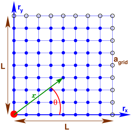
Figure 1: Sketch of a two-dimensional ($d=2$) square lattice with $n_{\mathrm{grid}}=L/a_{\mathrm{grid}}=2^{3}$. The filled circles indicate microcells of the principal box, the open circles some periodic images. The spatial position ${\bf r}$ of a microcell is either given by the $r_{x}$- and $r_{y}$-coordinates (in the principle box) or by the distance $r=|{\bf r}|$ from the origin (large circle) and the angle $\theta$.

We shall illustrate below various properties by means of (real and discrete) fields $f_{{\bf r}}$ (${\bf r}$ labeling the microcell position) corresponding to $N_{{\bf r}}$ microcells on regular grids in $d=2$ dimensions as sketched in Fig. 1. For simplicity we assume square periodic lattices of linear dimension $L=n_{\mathrm{grid}}a_{\mathrm{grid}}$, i.e. of ($d$-dimensional) volume $V=L^{d}=N_{{\bf r}}\delta V$ with $\delta V=a_{\mathrm{grid}}^{d}$ being the microcell volume. To characterize spatial correlations (cf. Sec. 2.4) it is convenient numrec to focus not on $f_{{\bf r}}$ but on its discrete Fourier transform

$$f_{{\bf q}}={\cal F}\{f_{{\bf r}}\}=\mathbf{E}^{{\bf r}}f_{{\bf r}}\exp(i{\bf q}\cdot{\bf r})$$ (11)

with $\mathbf{E}^{{\bf r}}$ being the average over all $N_{{\bf r}}$ microcells, using the notation Eq. (7), and ${\bf q}$ the discrete wavevectors (being commensurate with the periodic grid). Due to our Fourier transform convention the sum rule $f_{{\bf q}=0}=\mathbf{E}^{{\bf r}}f_{{\bf r}}$ holds. We denote by $f$ the field irrespective of its representation and specific values while $f_{{\bf r}}$ refers to the instantaneous field in real space and $f_{{\bf q}}$ to the corresponding discrete field in reciprocal space. Fast Fourier Transforms (FFT) numrec are naturally used for the efficient transformation between real and reciprocal space and it is thus convenient to set $n_{\mathrm{grid}}$ to be an integer power of $2$. Moreover, we set $a_{\mathrm{grid}}=1$, i.e. $L=n_{\mathrm{grid}}$ and $V=N_{{\bf r}}$.

LSM	description	$C[a]({\bf r})$	$C[b]({\bf r})$	$J$
A	uncorrelated sites	$a_{{\bf r}}\in{\cal U}[-0.1,0.1]$	$b_{{\bf r}}\in{\cal U}[0.1,1.9]$	0
B	exponential decay	$C[a]({\bf r})\approx c_{0}\exp(-r/\xi)$	$c_{{\bf r}}=a_{{\bf r}}$,$b_{{\bf r}}=1+c_{{\bf r}}^{2}$	0, 0.1, 1
C	power law decay	$C[a]({\bf r})\approx c_{0}/r^{\alpha}$ with $\alpha=1,2,3$	$c_{{\bf r}}=a_{{\bf r}}$,$b_{{\bf r}}=(1+0.1c_{{\bf r}})^{2}$	0
D	anisotropic decay	$C[a]({\bf q})=8\pi c_{0}(q_{x}q_{y}/q^{2})^{2}/N_{{\bf r}}$	$c_{{\bf r}}=a_{{\bf r}}$,$b_{{\bf r}}=(1+0.1c_{{\bf r}})^{2}$	$-1,0,\ldots,10$

Table 1: LSM variants studied with the third column indicating the imposed $C[a]({\bf r})$ and the forth $C[b]({\bf r})$. The uncorrelated random fields $a_{{\bf r}}$ and $b_{{\bf r}}$ of LSM-A are taken from the given uniform distributions ${\cal U}[\ldots]$. In all other cases $b_{{\bf r}}$ is computed using the indicated relation from an auxiliary field $c_{{\bf r}}$. Naturally, the inverse spring constant $b_{{\bf r}}=1/k_{{\bf r}}$ is always positive. The coupling parameter $J$ (fifth column) for springs of neighboring grid sites is switched off but for LSM-B and LSM-D. All correlations are isotropic for LSM-B and LSM-C while they are anisotropic for LSM-D.

2.3 Lattice spring model

We present below MC simulations of a “Lattice Spring Model” (LSM) with $x_{{\bf r}}$ being the linear length of the ideal springs and $a_{{\bf r}}$ and $b_{{\bf r}}=1/k_{{\bf r}}>0$ two quenched fields imposing, respectively, the average length of a spring and its variance. In addition, neighboring springs may be coupled by tuning a “coupling parameter” $J$. The energy $E_{{\bf r}}$ of a microcell at ${\bf r}$ is thus given by

$$E_{{\bf r}}=\frac{k_{{\bf r}}}{2}\left(x_{{\bf r}}-a_{{\bf r}}\right)^{2}+\frac{J}{2}\sum_{{\bf r}^{\prime}}(x_{{\bf r}^{\prime}}-x_{{\bf r}})^{2}$$ (12)

where the sum over ${\bf r}^{\prime}$ runs over the $2d$ nearest-neighbors of ${\bf r}$ on the periodic grid. In the limit where the interactions between springs are switched off ($J=0$) or are small, this implies the thermal averages $\left<x_{{\bf r}}\right>=a_{{\bf r}}$ and $\left<\delta x_{{\bf r}}^{2}\right>=b_{{\bf r}}T>0$ with $T$ being the temperature and setting Boltzmann’s constant $k_{\mathrm{B}}$ to unity. We impose $T=1$ in all presented simulations. A summary of the studied model variants is given in Table 1. How spatially correlated fields $f=a$ and $f=b$ are generated is explained in Sec. 2.6. Using these fields we perform Metropolis MC simulations with local moves LandauBinderBook ; AllenTildesleyBook . Results are recorded in time intervals $\delta\tau=10$ measured in MC steps.

2.4 Spatial correlation functions

In this work we shall impose or sample auto-correlation functions $C[f]({\bf r})=\langle K[f_{{\bf r}}]({\bf r})\rangle-\left<\mathbf{E}^{{\bf r}}f_{{\bf r}}\right>^{2}$ of various fields $f$. $\left<\ldots\right>$ stands here for some general average (to be specified below), ${\bf r}$ for any site (microcell) of the principal simulation box and

$$K[f_{{\bf r}}]({\bf r})\equiv\mathbf{E}^{{\bf r}^{\prime}}f_{{\bf r}+{\bf r}^{\prime}}f_{{\bf r}^{\prime}}$$ (13)

for the non-averaged correlation function of one given field $f_{{\bf r}}$. All correlation functions are even and periodic (Fig. 1). Periodicity is most readily implemented in reciprocal space using the Wiener-Khinchin theorem (WKT) numrec

$$K[f_{{\bf q}}]({\bf q})\equiv{\cal F}\{K[f_{{\bf r}}]({\bf r})\}=|f_{{\bf q}}|^{2}=f_{{\bf q}}f_{-{\bf q}}$$ (14)

for $f_{{\bf q}}={\cal F}\{f_{{\bf r}}\}$. The Fourier transformed auto-correlation functions are thus real and positive for all wavevectors ${\bf q}$.

All (averaged) correlation functions $C[f]({\bf r})$ or $C[f]({\bf q})$ considered here have in addition $x\leftrightarrow y$-symmetry, but are not necessarily radial symmetric (isotropic) spmP3 . Instead of the $d$-dimensional fields $C[f]({\bf r})$ we present below the weighted projections

$$C[f,p](r=|{\bf r}|)\equiv\left<C[f](r,\theta)\cos(2p\theta)\right>_{\theta}$$ (15)

averaged over all lattice sites (angles $\theta$) at the same (or similar) $r$ with $p=0,1,2,\ldots$ Due to the $x\leftrightarrow y$-symmetry only even $p=0,2,4,\ldots$ are allowed. We focus here on $p=0$ (“isotropic projection”) and $p=2$ (“anisotropic projection”) spmP3 . If not stated otherwise $p=0$ is assumed.

2.5 $V$-dependence of observables

As explained in the Introduction it is a general problem to explain or predict the system-size dependence of an observable ${\cal P}(V)$ for asymptotically large volumes $V$. The idea is to express ${\cal P}(V)^{2}=\mathbf{E}^{{\bf r}}C[f]({\bf r})$ as an average of a suitable correlation function $C[f]({\bf r})$ of a field $f$ which can be independently obtained numerically or understood on theoretical grounds. Using the isotropic ($p=0$) projection $C[f](r)$ of $C[f]({\bf r})$ we have

$$V\ {\cal P}(V)^{2}\approx I(V)\equiv\int\ \mathrm{d}r\ r^{d-1}\ C[f](r)$$ (16)

in $d$ dimensions. Let us write ${\cal P}(V)\sim 1/V^{\gamma}$ for large $V$ using the phenomenological exponent $\gamma$. Several cases are important. If $C[f](r)$ vanished more rapidly then $1/r^{d}$, the integral $I(V)$ is dominated by its lower bound and $V{\cal P}^{2}(V)$ becomes constant, hence, $\gamma=1/2$ if the lower bound does not explicitly dependent on $V$. If on the other hand $C[f](r)\simeq c_{0}>0$ for large $r$ with $c_{0}$ being a constant, $I(V)\simeq c_{0}V$ for large $V$ and, hence, $\gamma=0$ if $c_{0}$ is $V$-independent. More generally, LSM-C (Table 1) illustrates power-law correlations with

$$C[f](r)\simeq c_{0}/r^{\alpha}\mbox{ for }1\ll r\ll L/2$$ (17)

with $c_{0}$ being a $V$-independent constant. While (as already said) $\gamma=1/2$ for $\alpha>d$, this implies $\gamma=\alpha/2d<1/2$ for long-range correlations ($\alpha<d$), i.e. $\gamma\to 0$ for $\alpha\to 0$. Finally, we note that the intermediate case with $\alpha=d$ yields the logarithmic relation

$${\cal P}(V)\simeq\sqrt{(c_{1}+c_{2}\ln(V))/V}\mbox{ for }V\to\infty$$ (18)

with $c_{1}$ and $c_{2}>0$ being again $V$-independent constants.

2.6 Imposing $C[a]({\bf r})$ and $C[b]({\bf r})$

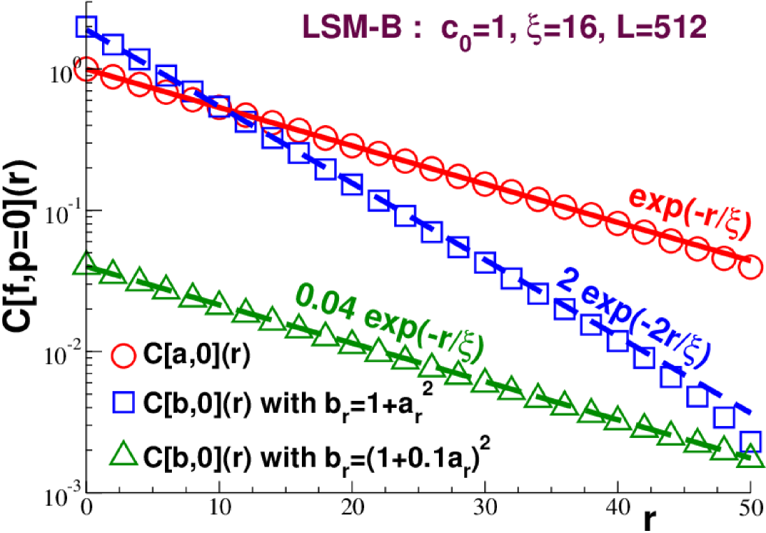
Figure 2: Isotropically averaged ($p=0$) correlation functions $C[f,p=0](r)$ for LSM-B with $c_{0}=1$, $\xi=16$ and $L=512$ characterizing the quenched fields $f=a$ and $f=b$ for all $J$. Note that $C[a,0](r)=\exp(-r/\xi)$ as imposed (bold solid line). For $f=b$ we compare the two closures $b_{{\bf r}}=1+a_{{\bf r}}^{2}$ (squares) and $b_{{\bf r}}=(1+0.1a_{{\bf r}})^{2}$. The dashed lines indicate the expected behavior for $L\gg\xi$.

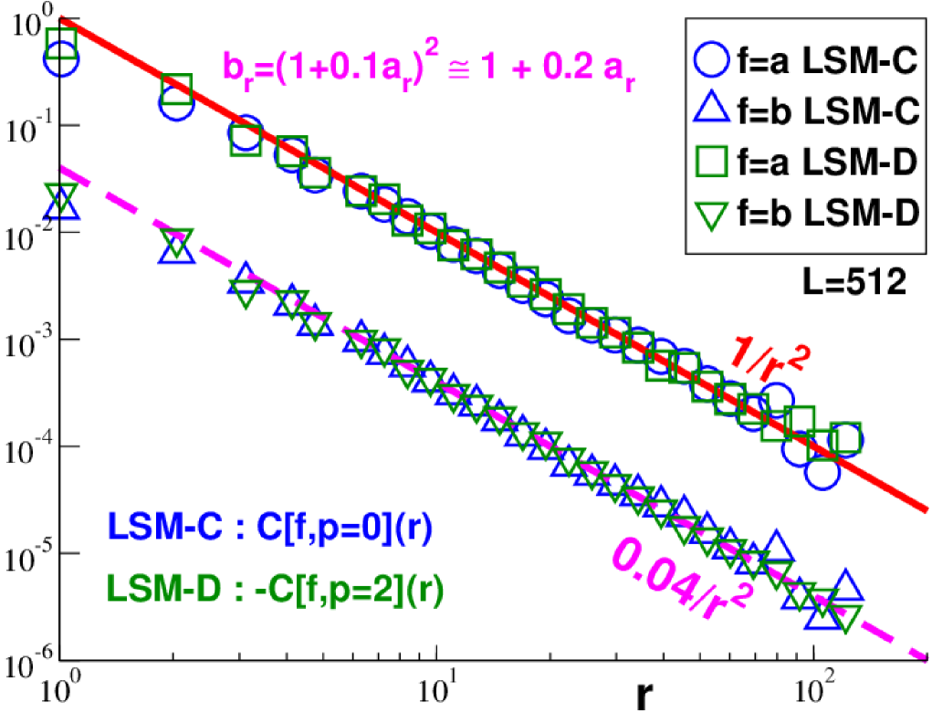
Figure 3: Double-logarithmic representation of $C[f,p=0](r)$ for LSM-C and $-C[f,p=2](r)$ for LSM-D for the two quenched fields $f=a$ and $f=b$ assuming that $b_{{\bf r}}=(1+0.1a_{{\bf r}})^{2}$.

As indicated in Table 1 the frozen fields $f=a$ and $f=b$ of LSM-A, our simplest LSM variant, are spatially decorrelated and uniformly distributed random variables. In all other considered cases these fields are spatially correlated as shown in Fig. 2 for LSM-B and in Fig. 3 for LSM-C and LSM-D. We explain here how this is done. We remind that, quite generally, a spatially correlated field with $C[f]({\bf r})=C_{\mathrm{imp}}({\bf r})$ is generated by setting FractalConcepts ; spmP3

$$f_{{\bf q}}=\sqrt{C_{\mathrm{imp}}({\bf q})N_{{\bf r}}}\ g_{{\bf q}}\mbox{ with }g_{{\bf q}}={\cal F}\{g_{{\bf r}}\}$$ (19)

being the Fourier transform of a (decorrelated) random Gaussian field $g_{{\bf r}}\in{\cal N}(0,1)$ of zero mean and unit variance. As a consequence

$$\left<|f_{{\bf q}}|^{2}\right>=C_{\mathrm{imp}}({\bf q})N_{{\bf r}}\left<g_{{\bf q}}g_{-{\bf q}}\right>=C_{\mathrm{imp}}({\bf q}),$$ (20)

i.e. according to the WKT we have $C[f]({\bf r})=C_{\mathrm{imp}}({\bf r})$ upon inverse Fourier transform back to real space. It is assumed here that (in addition of being even and periodic functions) the imposed $C_{\mathrm{imp}}({\bf q})$ must be for all ${\bf q}$ both real and positive in agreement with Eq. (14). If $C_{\mathrm{imp}}$ is known (stated) in real space, it may be thus necessary to regularize the desired relation. For instance, the power law $C_{\mathrm{imp}}({\bf r})=c_{0}/r^{\alpha}$ must be changed to

$$C_{\mathrm{imp}}({\bf r})=c_{0}(1+r^{2})^{-\alpha/2}$$ (21)

to avoid the singularity at the origin FractalConcepts . This is done, e.g., with $c_{0}=1$ and $\alpha=2$ for $f=a$ of LSM-C as shown in Fig. 3. To avoid such numerical problems $C_{\mathrm{imp}}({\bf q})$ is best directly imposed in reciprocal space. This is the case for $f=a$ and $f=b$ of LSM-D where we impose the anisotropic correlation function

$$C_{\mathrm{imp}}({\bf q})=8\pi\frac{c_{0}}{N_{{\bf r}}}\ (q_{x}q_{y}/q^{2})^{2}$$ (22)

($q_{x}$ and $q_{y}$ being the discrete components of the wavevector) motivated by the theoretically predicted shear-stress correlations of viscoelastic liquids and glasses Fuchs17 ; Fuchs18 ; Fuchs19 ; lyuda18 . As may be seen for $f=a$ of LSM-D in Fig. 3 (squares) Eq. (22) thus leads in real space to lyuda18

$$C({\bf r})=C_{\mathrm{imp}}({\bf r})=-2c_{0}\cos(4\theta)/r^{2}\mbox{ for }r>0,$$ (23)

i.e. the isotropic average vanishes (not shown) and the anisotropic average $C[f,p=2](r)=-c_{0}/r^{2}$ is long-ranged (bold solid line).

An additional problem arises for the correlated $f=b$ since all inverse spring constants $b_{{\bf r}}$ must be positive. To impose this we generate first an auxiliary field $c_{{\bf r}}$ using the above scheme. In all cases presented here $c_{{\bf r}}=a_{{\bf r}}$. From this $b_{{\bf r}}$ is obtained by setting, e.g., $b_{{\bf r}}=1+c_{{\bf r}}^{2}$. As seen in Fig. 2 this “closure” leads for LSM-B to $C[b]({\bf r})\approx 2\exp(-2r/\xi)$ for $L\gg\xi$ as can be also proved theoretically. Another possibility is to set

$$b_{{\bf r}}=(1+\lambda c_{{\bf r}})^{2}\approx 1+2\lambda c_{{\bf r}}\mbox{ for }|\lambda|\ll 1.$$ (24)

With $C[c]({\bf r})$ being the correlation function of the auxiliary variable this implies to leading order

$$C[b]({\bf r})\approx(2\lambda)^{2}C[c]({\bf r})\mbox{ for }|\lambda|\ll 1$$ (25)

which is merely a shift in logarithmic coordinates. That this works well can be seen (triangles) in Fig. 2 for LSM-B and in Fig. 3 for LSM-C and LSM-D.

3 Stochastic processes, observables and corresponding fields

3.1 Time-series and associated local fields

It is common to characterize a stochastic process $x(\tau)$ using ensembles $\{\mathbf{x}\}$ of discrete time-series

$$\mathbf{x}=\{x_{t}=x(\tau=t\delta\tau),t=1,\ldots,N_{\mathrm{t}}\}$$ (26)

with $t$ being the discrete time, $\delta\tau$ the time interval between the equidistant measurements and $\Delta\tau=N_{\mathrm{t}}\delta\tau$ the available “sampling time”. We assume that the global stochastic process is a $d$-dimensional volume average

$$x_{t}=\mathbf{E}^{{\bf r}}x_{t{\bf r}}\approx\frac{1}{V}\int\mathrm{d}{\bf r}\ x_{t{\bf r}}$$ (27)

over a discrete field $x_{t{\bf r}}$ of same dimension. As a specific example we consider the spatial average $x_{t}=\mathbf{E}^{{\bf r}}x_{t{\bf r}}$ of the LSM spring lengths $x_{t{\bf r}}$ (cf. Sec. 2.3). It is useful to directly measure $x_{t{\bf q}}={\cal F}\{x_{t{\bf r}}\}$ in reciprocal space. Since we consider stochastic processes in non-ergodic systems $\mathbf{x}_{ck}$, $x_{ckt}$, $x_{ckt{\bf r}}$ and $x_{ckt{\bf q}}$ are additionally characterized by the index $c$ of the independent configuration and the index $k$ of the time-series of a given $c$.

3.2 $t$-averaged observables and fields

Importantly, it is generally not possible to store all sets of time-series $\mathbf{x}$ and associated fields but one normally only computes and stores functionals (moments) ${\cal O}[\mathbf{x}]$ of each time-series, called here “$t$-averages” or “observables”. The two observables we shall focus on are the arithmetic mean

$${\cal O}[\mathbf{x}]=m[\mathbf{x}]\equiv\mathbf{E}^{t}x_{t}$$ (28)

and the empirical variance

$${\cal O}[\mathbf{x}]=v[\mathbf{x}]\equiv\beta V\ \mathbf{V}^{t}x_{t}$$ (29)

with $\beta=1/T$ being the inverse temperature ($k_{\mathrm{B}}=1$). The prefactor $\beta V$, introduced for consistency with previous work spmP1 ; spmP2 ; spmP3 , is natural for stochastic processes $x_{t}$ corresponding to intensive thermodynamic variables Lebowitz67 . We often write below compactly ${\cal O}_{ck}={\cal O}[\mathbf{x}_{ck}]$.

As already pointed out in the Introduction, we assume that, as the stochastic process $x_{t}$, also the observables ${\cal O}$ may be written as linear volume averages ${\cal O}[\mathbf{x}]=\mathbf{E}^{{\bf r}}{\cal O}_{{\bf r}}$ of local contributions ${\cal O}_{{\bf r}}$. For ${\cal O}[\mathbf{x}]=m[\mathbf{x}]$ these local contributions are given by ${\cal O}_{{\bf r}}=m_{{\bf r}}\equiv\mathbf{E}^{t}x_{t{\bf r}}$. Importantly, it is also possible to write the $t$-averaged variance as $v[\mathbf{x}]=\mathbf{E}^{{\bf r}}v_{{\bf r}}$ defining the “local variance”

$$v_{{\bf r}} \equiv \beta V\ \mathbf{E}^{t}(x_{t{\bf r}}-x_{{\bf r}})(x_{t}-x)$$ (30)

$$= \beta V\ \left(\mathbf{E}^{t}x_{t{\bf r}}x_{t}-x_{{\bf r}}x\right)$$

with $x_{{\bf r}}=\mathbf{E}^{t}x_{t{\bf r}}$ and $x=\mathbf{E}^{{\bf r}}x_{{\bf r}}$. Strictly speaking, $v_{{\bf r}}$ is a “co-variance” correlating the local field to the total average. Such local variances appear in the stress-fluctuation formulae for local elastic moduli Lutsko88 ; Lutsko89 ; Barrat06 . For numerical reasons it is convenient to compute the local fields $m_{{\bf r}}$ and $v_{{\bf r}}$ in Fourier space from $x_{t{\bf q}}$ using $m_{{\bf q}}=\mathbf{E}^{t}x_{t{\bf q}}$ and $v_{{\bf q}}=\beta V\mathbf{E}^{t}(x_{t{\bf q}}-x_{{\bf q}})(x_{t}-x)$ with $x=x_{{\bf q}={\bf 0}}$.

We remark finally that for the LSM versions with no or weak interactions between neighboring sites we have quite generally

$$m_{{\bf r}}\to a_{{\bf r}},v_{{\bf r}}\to b_{{\bf r}}\mbox{ for }J\to 0\mbox{ and }N_{\mathrm{t}}\to\infty.$$ (31)

In other words, since we know $C[a]({\bf r})$ and $C[b]({\bf r})$ by construction, Eq. (31) determines (for the specified limits) the spatial correlations for the local fields $m_{{\bf r}}$ and $v_{{\bf r}}$.

4 Global properties

4.1 Reminder of recent work

Summarizing recent work spmP2 ; spmP3 we discuss now several general properties of expectation values and variances of observables ${\cal O}_{ck}\equiv{\cal O}[\mathbf{x}_{ck}]$ in non-ergodic systems. We focus first on the dependences on the number $N_{\mathrm{c}}$ of independent configurations $c$ and the number $N_{\mathrm{k}}$ of time-series $k$ for each $c$ and discuss then the dependences on sampling time $\Delta\tau$ and volume $V$.

The first point to be made is that the total average ${\cal O}(N_{\mathrm{c}},N_{\mathrm{k}})$ of the ${\cal O}_{ck}$ can be obtained equivalently by

$${\cal O}(N_{\mathrm{c}},N_{\mathrm{k}})=\mathbf{E}^{c}\mathbf{E}^{k}{\cal O}_{ck}=\mathbf{E}^{k}\mathbf{E}^{c}{\cal O}_{ck}=\mathbf{E}^{l}{\cal O}_{l},$$ (32)

i.e. $c$- and $k$-averages commute and for such “simple averages” spmP2 the two indices $c$ and $k$ can be “lumped” together in one index $l$ with $N_{l}=N_{\mathrm{c}}N_{\mathrm{k}}$ as indicated by the last sum. The order of averaging matters, however, for the variance of ${\cal O}_{ck}$ for which three different definitions are relevant:

$$\delta{\cal O}^{2}_{\mathrm{tot}}(N_{\mathrm{c}},N_{\mathrm{k}}) \equiv \mathbf{V}^{l}{\cal O}_{l},$$ (33)

$$\delta{\cal O}^{2}_{\mathrm{int}}(N_{\mathrm{c}},N_{\mathrm{k}}) \equiv \mathbf{E}^{c}\mathbf{V}^{k}{\cal O}_{ck}\mbox{ and }$$ (34)

$$\delta{\cal O}^{2}_{\mathrm{ext}}(N_{\mathrm{c}},N_{\mathrm{k}}) \equiv \mathbf{V}^{c}\mathbf{E}^{k}{\cal O}_{ck}.$$ (35)

As shown in Ref. spmP2 , with these definitions Eq. (1) exactly holds. The “total variance” $\delta{\cal O}^{2}_{\mathrm{tot}}(N_{\mathrm{c}},N_{\mathrm{k}})$ is the standard commonly computed variance lyuda19a ; spmP1 ; Procaccia16 . We emphasize that $\delta{\cal O}^{2}_{\mathrm{tot}}(N_{\mathrm{c}},N_{\mathrm{k}})$ is again a “simple average”, i.e. all time-series $\mathbf{x}_{ck}$ are lumped together (index $l$) as for the average ${\cal O}(N_{\mathrm{c}},N_{\mathrm{k}})$, Eq. (32), while the order of the $c$- and $k$-averaging matters for the “internal variance” $\delta{\cal O}^{2}_{\mathrm{int}}(N_{\mathrm{c}},N_{\mathrm{k}})$ and the “external variance” $\delta{\cal O}^{2}_{\mathrm{ext}}(N_{\mathrm{c}},N_{\mathrm{k}})$.

Let us assume next that $N_{\mathrm{c}}$ becomes arbitrarily large. Importantly, the large-$N_{\mathrm{c}}$ limits ${\cal O}$ and $\delta{\cal O}_{\mathrm{tot}}$ of ${\cal O}(N_{\mathrm{c}},N_{\mathrm{k}})$ and $\delta{\cal O}_{\mathrm{tot}}(N_{\mathrm{c}},N_{\mathrm{k}})$ do neither depend on $N_{\mathrm{c}}$ nor on $N_{\mathrm{k}}$ and may, especially, also be computed by using only one time-series for each configuration ($N_{\mathrm{k}}=1$). At variance with this, internal and external variances still depend on $N_{\mathrm{k}}$, i.e. $\delta{\cal O}_{\mathrm{int}}(N_{\mathrm{c}},N_{\mathrm{k}})\to\delta{\cal O}_{\mathrm{int}}(N_{\mathrm{k}})$ and $\delta{\cal O}_{\mathrm{ext}}(N_{\mathrm{c}},N_{\mathrm{k}})\to\delta{\cal O}_{\mathrm{ext}}(N_{\mathrm{k}})$ in general for $N_{\mathrm{c}}\to\infty$. Note that

$$\delta{\cal O}_{\mathrm{int}}(N_{\mathrm{k}})\to 0,\delta{\cal O}_{\mathrm{ext}}(N_{\mathrm{k}})\to\delta{\cal O}_{\mathrm{tot}}\mbox{ for }N_{\mathrm{k}}\to 1.$$ (36)

For large spacer times $\tau_{\mathrm{spacer}}\gg\tau_{\mathrm{b}}$ between time-series the $N_{\mathrm{k}}$-dependence is given using Eq. (10) by spmP2

$$\delta{\cal O}^{2}_{\mathrm{int}}(N_{\mathrm{k}}) \simeq \left(1-\frac{1}{N_{\mathrm{k}}}\right)\ \delta{\cal O}^{2}_{\mathrm{int}}$$ (37)

$$\delta{\cal O}^{2}_{\mathrm{ext}}(N_{\mathrm{k}}) \simeq \delta{\cal O}^{2}_{\mathrm{ext}}+\frac{1}{N_{\mathrm{k}}}\ \delta{\cal O}^{2}_{\mathrm{int}}$$ (38)

where $\delta{\cal O}_{\mathrm{int}}$ and $\delta{\cal O}_{\mathrm{ext}}$ without the argument $N_{\mathrm{k}}$ stand for the limit $N_{\mathrm{k}}\to\infty$. Using these relations it is possible (with a bit of care as discussed in Sec. 4.2) to extrapolate internal and external variances measured at finite $N_{\mathrm{k}}$ to the respective large-$N_{\mathrm{k}}$ limits. We focus below on properties corresponding to the large-$N_{\mathrm{c}}$ and large-$N_{\mathrm{k}}$ limits.

The above properties may depend additionally on the sampling time $\Delta\tau$ and the volume $V$. The first dependence is relevant for all considered properties below and around the basin relaxation time $\tau_{\mathrm{b}}$. In this work we shall mainly focus on the opposite large-$\Delta\tau$ limit ($\Delta\tau\gg\tau_{\mathrm{b}}$). In this limit the typical $k$-averaged ${\cal O}_{ck}$ become $\Delta\tau$-independent. Hence, ${\cal O}(\Delta\tau,V)\to{\cal O}(V)$ and $\delta{\cal O}_{\mathrm{ext}}(\Delta\tau,V)\to\Delta_{\mathrm{ne}}(V)$ with $\Delta_{\mathrm{ne}}(V)$ being the “non-ergodicity parameter” defined in the Introduction, Eq. (2). At variance with this $\delta{\cal O}_{\mathrm{int}}(\Delta\tau,V)$ remains $\Delta\tau$-dependent decaying as

$$\delta{\cal O}_{\mathrm{int}}(\Delta\tau,V)\propto\sqrt{\tau_{\mathrm{b}}/\Delta\tau}\mbox{ for }\Delta\tau\gg\tau_{\mathrm{b}}$$ (39)

since we average over $\Delta\tau/\tau_{\mathrm{b}}$ independent subintervals spmP2 . Let us define the “non-ergodicity time” $\tau_{\mathrm{ne}}(V)\gg\tau_{\mathrm{b}}$ by $\delta{\cal O}_{\mathrm{int}}(\tau_{\mathrm{ne}},V)=\Delta_{\mathrm{ne}}(V)$. $\delta{\cal O}_{\mathrm{tot}}(\Delta\tau,V)$ is dominated by the internal fluctuations, Eq. (39), for $\Delta\tau\ll\tau_{\mathrm{ne}}(V)$ while

$$\delta{\cal O}_{\mathrm{tot}}(\Delta\tau,V)\to\delta{\cal O}_{\mathrm{ext}}(\Delta\tau,V)\approx\Delta_{\mathrm{ne}}(V)$$ (40)

in the large-$\Delta\tau$ limit ($\Delta\tau\gg\tau_{\mathrm{ne}}(V)$). If only the standard total variance is probed the non-ergodicity of the system may remain unnoticed for $\Delta\tau\ll\tau_{\mathrm{ne}}(V)$. As further emphasized below, it is then necessary to systematically check the $\Delta\tau$-dependence of $\delta{\cal O}_{\mathrm{tot}}(\Delta\tau,V)$ and to carefully extrapolate to $\Delta\tau\to\infty$ spmP2 ; spmP3 . The volume dependence will be addressed in more detail in Sec. 4.4. As a consequence $\tau_{\mathrm{ne}}(V)$ is found to strongly increase with $V$ since $\Delta_{\mathrm{ne}}(V)/\delta{\cal O}_{\mathrm{int}}(\Delta\tau,V)$ quite generally decreases with the system size. Assuming the latter ratio to decay as $1/V^{\gamma}$ this implies $\tau_{\mathrm{ne}}(V)\propto V^{2\gamma}$. The determination of $\Delta_{\mathrm{ne}}(V)$ by means Eq. (40) thus becomes increasingly difficult.

4.2 Focus and examples

We focus now on ${\cal O}[\mathbf{x}]=v[\mathbf{x}]$ and the corresponding expectation value $v(\Delta\tau,V)$, Eq. (32), and the three associated standard deviations $\delta v_{\mathrm{tot}}(\Delta\tau,V)$, $\delta v_{\mathrm{int}}(\Delta\tau,V)$ and $\delta v_{\mathrm{ext}}(\Delta\tau,V)$ determined according to Eqs. (33-35). We begin by discussing $\Delta\tau$-effects (Sec. 4.3) and turn then to the $V$-dependence of these properties (Sec. 4.4). We illustrate various points made above by means of MC simulations of the LSM introduced in Sec. 2. For all cases we have $T=1$, $\delta\tau=10$, $N_{\mathrm{c}}=200$ and at least $N_{\mathrm{k}}=100$. Using Eq. (37) and Eq. (38) we extrapolate to $N_{\mathrm{k}}\to\infty$. $\delta v_{\mathrm{int}}(\Delta\tau,V,N_{\mathrm{k}})$ can readily be extrapolated to $\delta v_{\mathrm{int}}(\Delta\tau,V)$ even using small $N_{\mathrm{k}}<10$ as discussed in Ref. spmP2 . At variance with this the extrapolation from $\delta v_{\mathrm{ext}}(\Delta\tau,V,N_{\mathrm{k}})$ to $\delta v_{\mathrm{ext}}(\Delta\tau,V)$ turns out to be inaccurate if the correction term

$$\frac{1}{N_{\mathrm{k}}}\delta v^{2}_{\mathrm{int}}(\Delta\tau,V)\propto\frac{\tau_{\mathrm{b}}}{N_{\mathrm{k}}\Delta\tau}\mbox{ for }\Delta\tau\gg\tau_{\mathrm{b}}$$ (41)

in Eq. (38) is not small compared to $\delta v^{2}_{\mathrm{ext}}(\Delta\tau,V,N_{\mathrm{k}})$. This matters especially for $\Delta\tau\ll 10^{3}$ and $J>0.1$ when the stochastic process becomes slow, increasing thus $\tau_{\mathrm{b}}(J)$. Occasionally, we have thus been forced to use $N_{\mathrm{k}}=1000$.

4.3 Sampling time dependence

Figure 4: Sampling time dependence of $v(\Delta\tau)$, $\delta v_{\mathrm{int}}(\Delta\tau)$, $\delta v_{\mathrm{ext}}(\Delta\tau)$ and $\delta v_{\mathrm{tot}}(\Delta\tau)$ for LSM-B with $\xi=1$, $J=0$ and $L=16$. It is seen that $\delta v_{\mathrm{int}}(\Delta\tau)\propto 1/\sqrt{\Delta\tau}$ (bold solid line) while all other properties become constant for large $\Delta\tau$. Note that $\delta v_{\mathrm{ext}}(\Delta\tau)\approx\Delta_{\mathrm{ne}}$ much faster than $\delta v_{\mathrm{tot}}(\Delta\tau)$.

As a generic example we present in Fig. 4 data obtained for LSM-B (exponentially decaying $a$- and $b$-fields) using a correlation length $\xi=1$ and a small simulation box with $L=16$. All interactions between neighboring springs $x_{{\bf r}}$ are switched off ($J=0$). As can be seen, $v(\Delta\tau)$, $\delta v_{\mathrm{int}}(\Delta\tau)$ and $\delta v_{\mathrm{ext}}(\Delta\tau)$ reach rapidly for $\Delta\tau\gg\tau_{\mathrm{b}}\approx 100$ the asymptotic behavior expected from the general discussion in Sec. 4.1, i.e. $v(\Delta\tau)$ and $\delta v_{\mathrm{ext}}(\Delta\tau)$ approach the respective constants $v$ and $\delta v_{\mathrm{ext}}=\Delta_{\mathrm{ne}}$ while $\delta v_{\mathrm{int}}(\Delta\tau)\propto 1/\sqrt{\Delta\tau}$ (bold solid line). Importantly, due to Eq. (1)

$$\delta v_{\mathrm{tot}}(\Delta\tau,V)=\sqrt{\delta v^{2}_{\mathrm{int}}(\Delta\tau,V)+\delta v^{2}_{\mathrm{ext}}(\Delta\tau,V)}$$ (42)

approaches $\Delta_{\mathrm{ne}}$ much later than $\delta v_{\mathrm{ext}}(\Delta\tau)$, i.e. only for $\Delta\tau\gg\tau_{\mathrm{ne}}\approx 5600\gg\tau_{\mathrm{b}}$. For this reason it is problematic to determine $\Delta_{\mathrm{ne}}$ only by measuring $\delta v_{\mathrm{tot}}(\Delta\tau)$ for one sampling time.

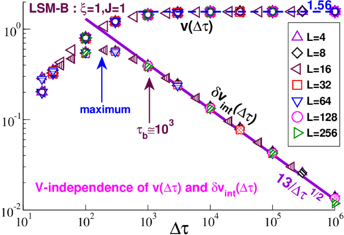
Figure 5: $v(\Delta\tau)$ (upper data with open symbols) and $\delta v_{\mathrm{int}}(\Delta\tau)$ (symbols filled with pattern) for LSM-B with $\xi=1$ and $J=1$ for a broad range of $L$ demonstrating the $V$-independence of both properties. Increasing $J$ increases $\tau_{\mathrm{b}}$, decreases $v$ (horizontal dashed line) and increases the power-law amplitude for $\delta v_{\mathrm{int}}(\Delta\tau)\simeq 1/\sqrt{\Delta\tau}$ for $\Delta\tau\gg\tau_{\mathrm{b}}$ (bold solid line).

Deviations from this generic asymptotic behavior are visible for small $\Delta\tau$ around and below the basin relaxation time $\tau_{\mathrm{b}}$. This can be seen from Fig. 4 but more clearly from Fig. 5 where we present $v(\Delta\tau)$ and $\delta v_{\mathrm{int}}(\Delta\tau)$ for LSM-B with $J=1$ and for a broad range of system-sizes. Remarkably, $\delta v_{\mathrm{int}}(\Delta\tau)$ reveals non-monotonic behavior with a maximum below the basin relaxation time $\tau_{\mathrm{b}}(J=1)\approx 10^{3}$. Being generally due to relaxation processes within each meta-basin this small-$\Delta\tau$ regime is more relevant for more realistic models as discussed elsewhere lyuda19a ; spmP1 ; spmP2 . For the present work it is only important to stress that the general $\Delta\tau$-dependence of $v(\Delta\tau)$ and $\delta v_{\mathrm{int}}(\Delta\tau)$ can be traced back to the “mean-square displacement” (MSD) $h(\tau)$ of the stochastic process. This is defined by

$$h(\tau=t\delta\tau)\equiv h_{t=|i-j|}\equiv\frac{\beta V}{2}\left<(x_{i}-x_{j})^{2}\right>$$ (43)

averaged over all time entries $i$ and $j$ of a long trajectory with $t=|i-j|$. For stationary processes spmP1

$$v(\Delta\tau)=\frac{2}{N_{\mathrm{t}}^{2}}\sum_{t=1}^{N_{\mathrm{t}}-1}(N_{\mathrm{t}}-t)\ h_{t}$$ (44)

must hold. The sampling time dependence of $\delta v_{\mathrm{int}}(\Delta\tau)$ can be understood and described assuming a stationary Gaussian stochastic process lyuda19a ; spmP1 ; spmP2 . This implies that

$$\delta v^{2}_{\mathrm{int}}(\Delta\tau) = \delta v^{2}_{\mathrm{G}}[h]\equiv\frac{1}{2N_{\mathrm{t}}^{4}}\sum_{i,j,k,l=1}^{N_{\mathrm{t}}}\ g_{ijkl}^{2}\mbox{ with }$$ (45)

$$g_{ijkl} \equiv (h_{i-j}+h_{k-l})-(h_{i-l}+h_{j-k}).$$

Numerical more convenient alternative representations are given elsewhere lyuda19a ; spmP1 . By analyzing the functional $\delta v_{\mathrm{G}}[h]$ it is seen lyuda19a ; spmP1 that while $\delta v_{\mathrm{int}}(\Delta\tau)\propto 1/\sqrt{\Delta\tau}$ for (to leading order) $h(t)\approx const$ for $t\approx\Delta\tau$, it may become large with $\delta v_{\mathrm{int}}(\Delta\tau)\approx v(\Delta\tau)$ for sampling times $\Delta\tau$ corresponding to a strong change of $h(t\approx\Delta\tau)$. We emphasize finally that since $h(\tau)$, $v(\Delta\tau)$ and $\delta v_{\mathrm{int}}(\Delta\tau)$ are connected through Eq. (44) and Eq. (45) all three quantities must have the same system-size dependence and this for all times. That $v(\Delta\tau)$ and $\delta v_{\mathrm{int}}(\Delta\tau)$ in Fig. 5 are both $V$-independent is one consequence.

4.4 Volume dependence

We turn now to system-size effects. Let us focus first on the limit $\Delta\tau\gg\tau_{\mathrm{ne}}(V)$ where $\delta v_{\mathrm{int}}(\Delta\tau)$ becomes negligible and $\delta v_{\mathrm{tot}}(\Delta\tau)\approx\delta v_{\mathrm{ext}}(\Delta\tau)\approx\Delta_{\mathrm{ne}}$. Examples for $v(V)$ and $\Delta_{\mathrm{ne}}(V)$ are given for $J=0$ in Fig. 6 and Fig. 7 and for $\Delta_{\mathrm{ne}}(V)$ comparing different $J$ for LSM-D in Fig. 8.

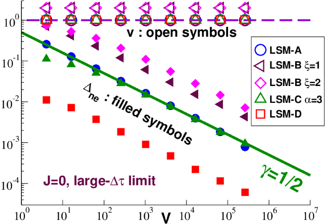
Figure 6: $V$-dependence for $v$ and $\Delta_{\mathrm{ne}}$ (filled symbols) for LSM-A, LSM-B with $\xi=1$ and $\xi=2$, LSM-C with $\alpha=3$ and LSM-D. $v$ is always $V$-independent (horizontal dashed line) and $\Delta_{\mathrm{ne}}\propto 1/V^{\gamma}$ with $\gamma=1/2$ (bold solid line) for the given examples with short-range correlations. $\Delta_{\mathrm{ne}}(V)$ for LSM-D (filled squares) is finite, but much smaller than all other cases.

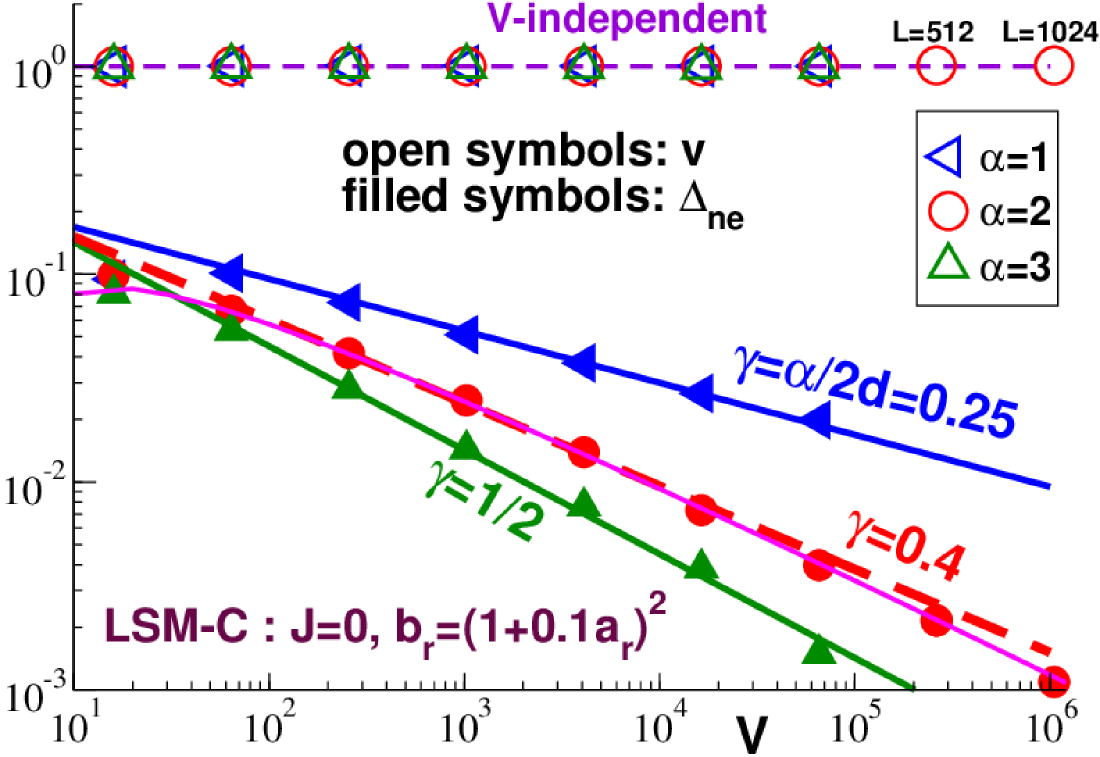
Figure 7: Volume dependence of $v$ and $\Delta_{\mathrm{ne}}$ for LSM-C and three different values of $\alpha$. We observe short-range behavior with $\gamma=1/2$ for $\alpha>d$, long range behavior with $\gamma=\alpha/2d$ for $\alpha<d$ and, as expected from Eq. (18), logarithmic decay (thin solid line) for the intermediate case with $\alpha=d=2$. The latter case is well fitted by an exponent $\gamma=0.4$ (bold dashed line).

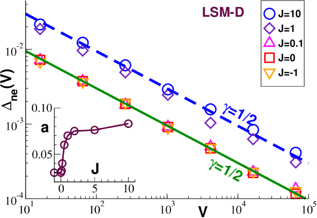
Figure 8: $\Delta_{\mathrm{ne}}(V,J)$ for LSM-D for different $J$. Main panel: $\gamma=1/2$ holds for all $J$ (lines). Inset: Power-law amplitude $a(J)\equiv\Delta_{\mathrm{ne}}(V,J)V^{1/2}$ vs. coupling constant $J$. Apparently, the spring coupling introduces isotropic ($p=0$) correlations of the $x_{t{\bf r}}$- and, hence, $v_{{\bf r}}$-fields which remain, however, short-ranged.

The first point to be made is that the variance $v$ is always $V$-independent (as already seen in Fig. 5) due to the prefactor $\beta V$ introduced in Eq. (29). In fact this scaling is expected to hold for all stochastic processes describing intensive system properties if the $c$-trajectories are at thermal equilibrium in their respective basins spmP2 . (Note that each stochastic process is ergodic in its basin.) Using the standard fluctuation-dissipation relation for the fluctuation of intensive thermodynamic variables Lebowitz67 ; WXP13 ; AllenTildesleyBook this implies that $v_{c}$ does not depend explicitly on $V$ and, hence, neither does $v=\mathbf{E}^{c}v_{c}$. This argument even holds for systems with long-range correlations if standard thermostatistics can be used for each basin. This can be seen from the variances $v$ of LSM-C (power-law correlations) for exponents $\alpha<d$ as shown in Fig. 7 for $\alpha=1$.

Interestingly, the same thermodynamic reasoning cannot be made for $\Delta_{\mathrm{ne}}$. However, it can be readily demonstrated that quite generally $\Delta_{\mathrm{ne}}\propto 1/V^{\gamma}$ with $\gamma=1/2$ for systems without spatial correlations spmP2 . This is the case for LSM-A with $J=0$ on which we may focus without loss of generality. According to Eq. (31) we have $b_{c{\bf r}}=v_{c{\bf r}}$ and thus $v_{c}=\mathbf{E}^{{\bf r}}v_{c{\bf r}}$ is given by the spatial average $b_{c}=\mathbf{E}^{{\bf r}}b_{c{\bf r}}$. This implies in turn that $v\equiv\mathbf{E}^{c}v_{c}=\mathbf{E}^{c}b_{c}\equiv b$. To get the variance of the variance $\mathbf{V}^{c}v_{c}$ one uses again that the variance of the sum of stochastic independent variables is the sum of the variances of those variables

$$\Delta_{\mathrm{ne}}^{2}=\mathbf{V}^{c}v_{c}=\mathbf{V}^{c}\left(\frac{1}{N_{{\bf r}}}\sum_{{\bf r}}b_{c{\bf r}}\right)=\frac{1}{N_{{\bf r}}}\times\underline{\mathbf{E}^{{\bf r}}\mathbf{V}^{c}b_{c{\bf r}}}$$ (46)

and the fact that the underlined term does not depend on the number of grid sites $N_{{\bf r}}\propto V$ for large systems. Hence, $\gamma=1/2$. Naturally, this does not only hold for systems with strictly decorrelated fields but also if short-range correlations are present (which may be renormalized away) as confirmed by the various additional examples with short-range correlations presented in Fig. 6, Fig. 7 and Fig. 8. (As shown in the latter plot for LSM-D, the coupling parameter $J$ has apparently only a weak quantitative effect on the range of the effective spatial correlations.) The above argument breaks down, however, if long-range correlations are present as for the power-law exponent $\alpha=1$ of LSM-C shown in Fig. 7. The observed power law with $\gamma=\alpha/2d$ is, of course, expected from Sec. 2.5 as we shall corroborate below in Sec. 5.

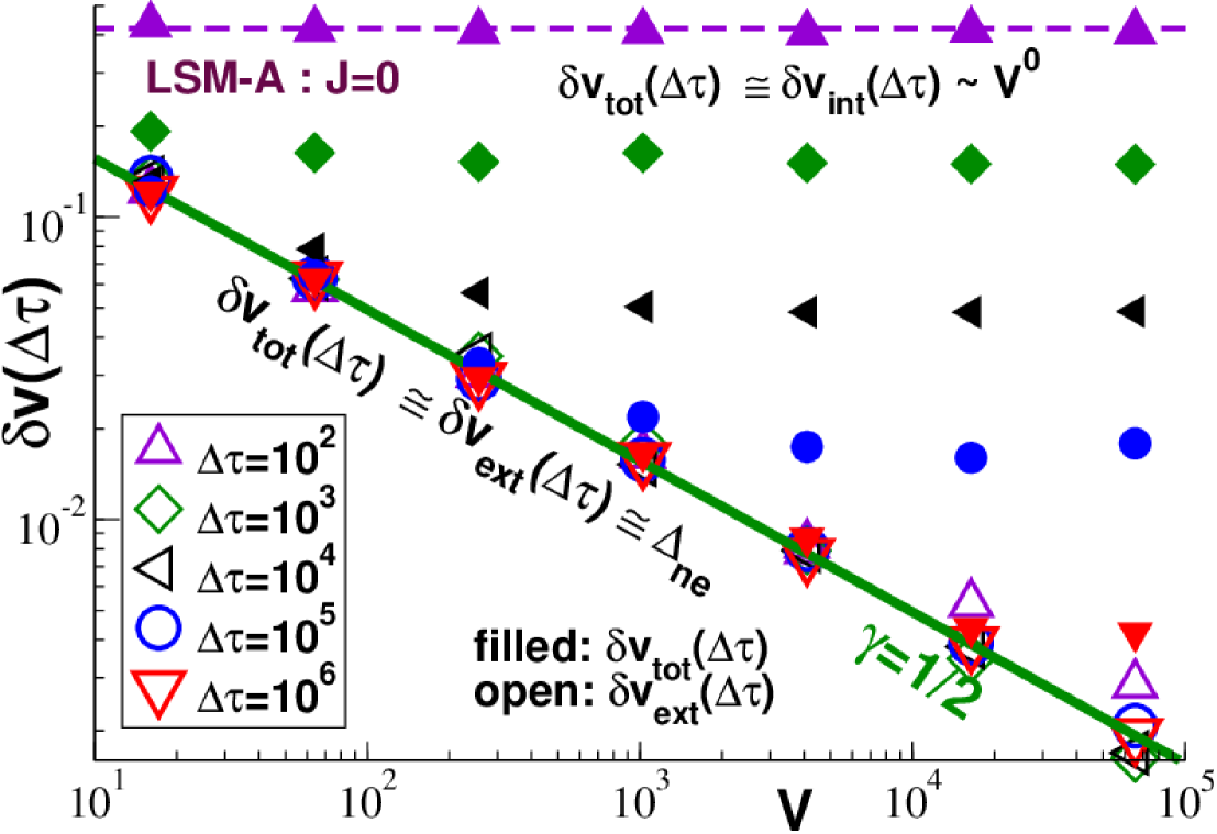
Figure 9: $V$-dependence of $\delta v_{\mathrm{tot}}(\Delta\tau)$ and $\delta v_{\mathrm{ext}}(\Delta\tau)$ for LSM-A for different sampling times $\Delta\tau$ as indicated. The bold green line indicates the known $\Delta_{\mathrm{ne}}\propto 1/V^{\gamma}$ with $\gamma=1/2$. While $\delta v_{\mathrm{ext}}(\Delta\tau,V)\approx\Delta_{\mathrm{ne}}(V)$ for all $L$ and $\Delta\tau\gg\tau_{\mathrm{b}}\approx 10$, a much slower convergence to this limit is seen for $\delta v_{\mathrm{tot}}(\Delta\tau,V)$ due to the $V$-independent contribution $\delta v_{\mathrm{int}}(\Delta\tau)$ to $\delta v_{\mathrm{tot}}(\Delta\tau)$.

Let us instead end this paragraph with some comments on the $\Delta\tau$-dependence of the system-size effects. We remind that $v(\Delta\tau)$, $\delta v_{\mathrm{int}}(\Delta\tau)$ and $h(t)$ are related via Eq. (44) and Eq. (45). In view of the observed $V$-independence of $v$ it is thus not surprising that $v(\Delta\tau)$ and $\delta v_{\mathrm{int}}(\Delta\tau)$ are found to be $V$-independent for all $\Delta\tau$ as shown in Fig. 5. Since $\delta v_{\mathrm{int}}(\Delta\tau)\propto V^{0}/\sqrt{\Delta\tau}$ for $\Delta\tau\gg\tau_{\mathrm{b}}$ the non-ergodicity crossover time $\tau_{\mathrm{ne}}(V)\simeq V^{2\gamma}$ rapidly increases with $V$. This implies that the regime with $\tau_{\mathrm{b}}\ll\Delta\tau\ll\tau_{\mathrm{ne}}(V)$ where $\delta v_{\mathrm{tot}}(\Delta\tau)\approx\delta v_{\mathrm{int}}(\Delta\tau)$ strongly increases with $V$. If computed at constant $\Delta\tau$ as in most computational studies Procaccia16 , $\delta v_{\mathrm{tot}}(\Delta\tau,V)$ as a function of $V$ must thus become $V$-independent for large $V$. This behavior can clearly be seen from the data presented in Fig. 9 for LSM-A (filled symbols). The crossing over from $\delta v_{\mathrm{tot}}(\Delta\tau,V)\approx\Delta_{\mathrm{ne}}(V)\propto 1/V^{\gamma}$ for small $V$ (bold solid line) to $\delta v_{\mathrm{tot}}(\Delta\tau,V)\approx\delta v_{\mathrm{int}}(\Delta\tau)\propto V^{0}$ for large $V$ makes it likely that in turn a too small apparent exponent $\gamma$ may be fitted. Should $\delta v_{\mathrm{ext}}(\Delta\tau,V)$ not be available one needs at least to compare $\delta v_{\mathrm{tot}}(\Delta\tau,V)$ for several $\Delta\tau$. Only the $V$-regime where the highest $\Delta\tau$-data do indeed collapse can be used for a fit of the exponent $\gamma$. Without such a crosscheck all fits claiming an exponent $\gamma<1/2$ and, hence, (according to the preceding paragraph) long-range spatial correlations are questionable.

5 Associated spatial correlation functions

5.1 General relations for non-ergodic systems

As demonstrated in detail in Appendix A the integrals, Eqs. (3-5), are solved by

$$C_{\mathrm{tot}}({\bf q}) = \mathbf{E}^{l}K[{\cal O}_{l{\bf q}}]({\bf q})-{\cal O}^{2}\delta_{{\bf q}{\bf 0}}$$ (47)

$$C_{\mathrm{int}}({\bf q}) = \mathbf{E}^{c}\mathbf{E}^{k}K[{\cal O}_{ck{\bf q}}-{\cal O}_{c{\bf q}}]({\bf q})$$ (48)

$$C_{\mathrm{ext}}({\bf q}) = \mathbf{E}^{c}K[{\cal O}_{c{\bf q}}]({\bf q})-{\cal O}^{2}\delta_{{\bf q}{\bf 0}}$$ (49)

where for numerical convenience we have stated all correlation functions in reciprocal space (with $\delta_{{\bf q}{\bf 0}}$ denoting Kronecker’s symbol for the zero-wavevector contribution). The “simple average” $C_{\mathrm{tot}}$ corresponds to the standard commonly measured correlation function. The internal correlation function $C_{\mathrm{int}}$ characterizes the correlations of the difference ${\cal O}_{ck{\bf q}}-{\cal O}_{c{\bf q}}$ with respect to the $k$-average ${\cal O}_{c{\bf q}}=\mathbf{E}^{k}{\cal O}_{ck{\bf q}}$. Moreover, as shown by Eq. (71) the “total” correlation function $C_{\mathrm{tot}}$ is the sum of an “internal” contribution $C_{\mathrm{int}}$ and an “external” contribution $C_{\mathrm{ext}}$

$$C_{\mathrm{tot}}({\bf q})=C_{\mathrm{int}}({\bf q})+C_{\mathrm{ext}}({\bf q})$$ (50)

in agreement with Eq. (6) stated in the Introduction.

Just as $\delta{\cal O}_{\mathrm{tot}}$, $\delta{\cal O}_{\mathrm{int}}$ and $\delta{\cal O}_{\mathrm{ext}}$ the correlation functions $C_{\mathrm{tot}}$, $C_{\mathrm{int}}$ and $C_{\mathrm{ext}}$ depend in general on $N_{\mathrm{c}}$ and $N_{\mathrm{k}}$. As above in Sec. 4.1 we assume that $N_{\mathrm{c}}$ is arbitrarily large. This implies that

$$\lim_{N_{\mathrm{c}}\to\infty}C_{\mathrm{tot}}({\bf q},N_{\mathrm{c}},N_{\mathrm{k}})=C_{\mathrm{tot}}({\bf q})$$ (51)

and similarly in real space, i.e. not only the $N_{\mathrm{c}}$- but also the $N_{\mathrm{k}}$-dependence drops out since the total correlation function is a simple $l$-average. Consistently with Eq. (37) we have for the internal correlation function

$$C_{\mathrm{int}}({\bf q},N_{\mathrm{k}})\simeq\left(1-\frac{1}{N_{\mathrm{k}}}\right)C_{\mathrm{int}}({\bf q})$$ (52)

for $N_{\mathrm{c}}\to\infty$. Using Eq. (51), Eq. (52) together with Eq. (6) it is then seen that

$$C_{\mathrm{ext}}({\bf q},N_{\mathrm{k}})\simeq C_{\mathrm{ext}}({\bf q})+\frac{1}{N_{\mathrm{k}}}C_{\mathrm{int}}({\bf q}).$$ (53)

These two relations should be used to extrapolate for the asymptotic $C_{\mathrm{int}}({\bf q})$ and $C_{\mathrm{ext}}({\bf q})$ using the $C_{\mathrm{int}}({\bf q},N_{\mathrm{k}})$ and $C_{\mathrm{ext}}({\bf q},N_{\mathrm{k}})$ measured at finite $N_{\mathrm{k}}$. While the $N_{\mathrm{k}}$-dependent correction term is less crucial for $C_{\mathrm{int}}({\bf q},N_{\mathrm{k}})$, it is important, as above for $\delta{\cal O}_{\mathrm{ext}}(N_{\mathrm{k}})$, to take advantage of Eq. (53), especially if $C_{\mathrm{int}}({\bf q})$ is large. We focus below on the $N_{\mathrm{k}}$-extrapolated correlation functions in real space.

The correlation functions may a priori also depend explicitly on the sampling time $\Delta\tau$ and the system volume $V$. One trivial reason for a $V$-dependency is that the linear box length $L$ sets a cut-off. Fortunately, this only matters for large distances $r\approx L/2$ (and for the corresponding small wavevectors), i.e. this effect becomes irrelevant for large $L$ as one verifies by systematically increasing the box size. Since $\delta{\cal O}_{\mathrm{ext}}(\Delta\tau,V)$ becomes $\Delta\tau$-independent and $\delta{\cal O}_{\mathrm{int}}(\Delta\tau,V)\propto 1/\sqrt{\Delta\tau}$ for $\Delta\tau\gg\tau_{\mathrm{b}}$ this naturally suggests

$$\left.\begin{array}[]{ll}C_{\mathrm{ext}}({\bf r},\Delta\tau,V)\simeq&C_{\mathrm{ext}}({\bf r},V)\\ C_{\mathrm{int}}({\bf r},\Delta\tau,V)\propto&1/\Delta\tau\end{array}\right\}\mbox{ for }\Delta\tau\gg\tau_{\mathrm{b}}$$ (54)

as discussed theoretically in more detail in Appendix A.3 and Appendix B. We shall verify numerically in the next subsection whether this holds for our model systems.

5.2 Examples for lattice spring models

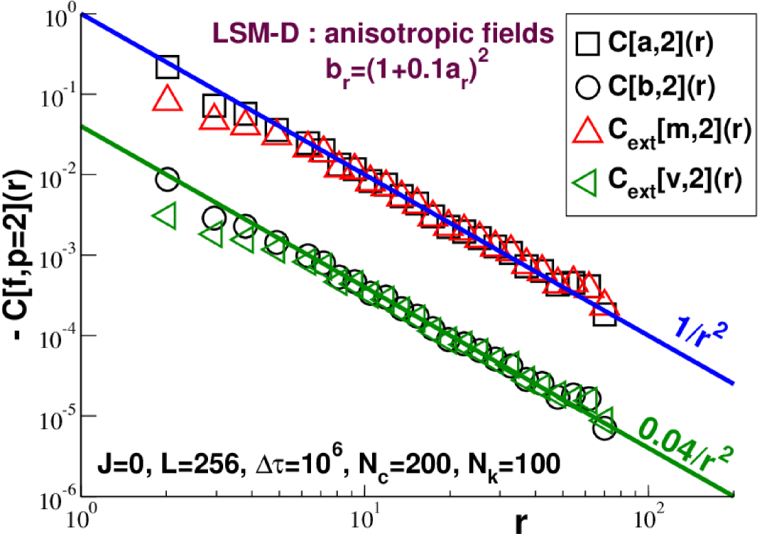
Figure 10: $-C[f,p=2](r)$ for LSM-D for $J=0$ and $\Delta\tau\gg\tau_{\mathrm{ne}}\gg\tau_{\mathrm{b}}$ confirming that $C[a]({\bf r})\approx C_{\mathrm{ext}}[m]({\bf r})$ and $C[b]({\bf r})\approx C_{\mathrm{ext}}[v]({\bf r})$ as expected from Eq. (31).

We present now various (projected) correlation functions $C[f,p](r)$ from our LSM simulations. We begin in Fig. 10 with data from LSM-D obtained for $J=0$ and a large sampling time $\Delta\tau=10^{6}$. We remind that LSM-D is defined by Eq. (23) for the $a$-field and by Eq. (24) for the $b$-field. All indicated correlation functions are obtained by anisotropic projection ($p=2$). Since all spring interactions are switched off ($J=0)$ and since $\Delta\tau\gg\tau_{\mathrm{b}}$ we have $m_{{\bf r}}\approx a_{{\bf r}}$ and $v_{{\bf r}}\approx b_{{\bf r}}$. As expected from Eq. (23) and Eq. (25), Fig. 10 confirms

$$-C_{\mathrm{ext}}[m,p](r) \approx -C[a,p](r)\approx 1/r^{2}$$ (55)

$$-C_{\mathrm{ext}}[v,p](r) \approx -C[b,p](r)\approx(2\lambda)^{2}/r^{2}$$ (56)

with $p=2$ and $\lambda=0.1$. Similar results have been found for all model cases with $|J|\ll 1$ and $\Delta\tau\gg\tau_{\mathrm{b}}$. Since, moreover, $\Delta\tau\gg\tau_{\mathrm{ne}}$ for the presented data, the internal correlation functions $C_{\mathrm{int}}[f]({\bf r},\Delta\tau)$ are negligible small and $C_{\mathrm{tot}}[f]({\bf r},\Delta\tau)\approx C_{\mathrm{ext}}[f]({\bf r})$ holds (not shown).

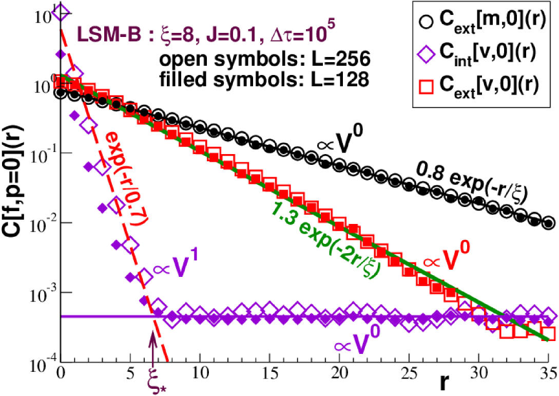
Figure 11: Isotropic projection $C[f,p=0](r)$ for LSM-B with $\xi=8$, $J=0.1$ and $\Delta\tau=10^{5}$. Open symbols refer to $L=256$, small filled symbols to $L=128$. As expected $C_{\mathrm{ext}}[m](r)$ and $C_{\mathrm{ext}}[v](r)$ decrease exponentially just as $C[a](r)$ and $C[b](r)$. $C_{\mathrm{int}}[v](r)$ decays exponentially (dashed line) for $r\ll\xi_{\star}$ ($\xi_{\star}$ being a crossover length) but becomes constant for large $r$.

All correlation functions presented below in this section are isotropically projected. “$p=0$” is often suppressed for clarity. We consider now finite spring interactions and smaller sampling times. As an example we show in Fig. 11 correlation functions obtained for LSM-B with $\xi=8$, $J=0.1$ and $\Delta\tau=10^{5}$. Data for two system sizes are compared. $C_{\mathrm{ext}}[m](r)$ and $C_{\mathrm{ext}}[v](r)$ are $V$-independent for all $r\ll L/2$. The small, finite $J$ only has a minor effect on the prefactors: As for $J=0$ we observe $C_{\mathrm{ext}}[m](r)\approx C[a](r)\approx\exp(-r/\xi)$ and $C_{\mathrm{ext}}[v](r)\approx C[b](r)\approx\exp(-2r/\xi)$. The observed short-range correlations are consistent with $\gamma=1/2$ (cf. Fig. 6).

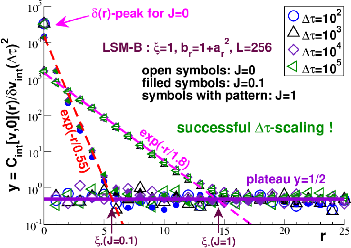
Figure 12: $y=C_{\mathrm{int}}[v,0](r)/\delta v^{2}_{\mathrm{int}}(\Delta\tau)$ versus $r$ for LSM-B ($\xi=1$, $L=256$) with $J=0$ (open symbols), $J=0.1$ (filled symbols) and $J=1$ (symbols with pattern). Data from a broad $\Delta\tau$-range scale nicely for each $J$. Note the huge peak at $r=0$ (arrow) for $J=0$ and the exponential decays (dashed lines) with $y(r)\sim V\exp(-r/\xi_{\mathrm{ind}})$ for $J>0$ and $r\ll\xi_{\star}(J)$. For large $r$ all data approach $y=1/2$ (bold horizontal line).

We turn next to the scaling of the internal correlation function $C_{\mathrm{int}}[v](r)$. Focusing on LSM-B this is presented in Fig. 11 and Fig. 12. As we shall see, all our numerical data are consistent with the general scaling

$$C_{\mathrm{int}}[v](r,\Delta\tau,V)=[V(1-\alpha)c(r)+\alpha]\ \delta v^{2}_{\mathrm{int}}(\Delta\tau)$$ (57)

with $\alpha=1/2$ and $c(r)$ being a $\Delta\tau$-independent function, depending somewhat on the model (especially on the coupling parameter $J$), vanishing for large distances $r$ and being normalized as $V\mathbf{E}^{{\bf r}}c({\bf r})=1$. In fact, this scaling is natural for a large class of models as further discussed in Appendix B.

Let us focus first on the $\Delta\tau$-dependence of the internal correlation function. We present in Fig. 12 the rescaled correlation function $y=C_{\mathrm{int}}[v](r)/\delta v^{2}_{\mathrm{int}}(\Delta\tau)$ as a function of $r$ for LSM-B with $J=0$, $J=0.1$ and $J=1$. A perfect data collapse is observed for each $J$ confirming thus Eq. (57). Since $\delta v^{2}_{\mathrm{int}}(\Delta\tau)\propto 1/\Delta\tau$ for the presented sampling times, we could have also used as vertical axis $C_{\mathrm{int}}[v](r,\Delta\tau)\times\Delta\tau$ to scale the data. Importantly, the dimensionless scaling variable $y$ is more general allowing the scaling for all $\Delta\tau$, i.e. also for $\Delta\tau\ll\tau_{\mathrm{b}}$.

Turning to the $r$-dependence we note that Eq. (57) implies that $C_{\mathrm{int}}[v](r,\Delta\tau,V)$ should level off to a plateau with $\alpha\delta v^{2}_{\mathrm{int}}(\Delta\tau)>0$ for sufficiently large $r\gg\xi_{\star}$. As emphasized by the bold horizontal lines in Fig. 11 and Fig. 12 this is indeed the case. Moreover, the latter figure confirms $\alpha=1/2$, i.e. quite generally we have $C_{\mathrm{int}}[v](r)\to\delta v^{2}_{\mathrm{int}}(\Delta\tau)/2$ for large $r$. That $C_{\mathrm{int}}[v](r)$ becomes a finite constant for large $r$, albeit the instantaneous $x_{t{\bf r}}$-field is decorrelated, has to do with the definition of the $v_{{\bf r}}$-field, Eq. (30), as further explained in Appendix B.1. As can be seen from the latter calculation the function $c(r)$ for LSM-A with $J=0$ has a jump singularity at $r=0$, Eq. (96). That this is also the case for all other models with $J=0$ can be seen for LSM-B in Fig. 12 (arrow). This becomes different if the interaction between the springs is switched on ($J>0$). As seen in Fig. 11 and Fig. 12 we then observe for $r\ll\xi_{\star}$ a continuous exponential decay $C_{\mathrm{int}}[v](r)\propto c(r)\propto\exp(-r/\xi_{\mathrm{ind}})$ with a finite induced correlation length $\xi_{\mathrm{ind}}$ weakly increasing with $J$.

Moreover, as can be also seen in Fig. 11, the internal correlations increase in the first $r$-regime with $V$. Confirming the $V$-dependence indicated in Eq. (57), a systematic comparison of a broad range of $L$ reveals that $C_{\mathrm{int}}[v](r)\propto V$ for small $r$ while it is strictly $V$-independent for large $r$ (not shown). Due to both contributions the volume average $\mathbf{E}^{{\bf r}}C_{\mathrm{int}}[v]({\bf r})$ is thus $V$-independent consistently with the $V$-independence of $\delta v^{2}_{\mathrm{int}}(\Delta\tau)$ demonstrated above (cf. Fig. 5 and Sec. 4.4).

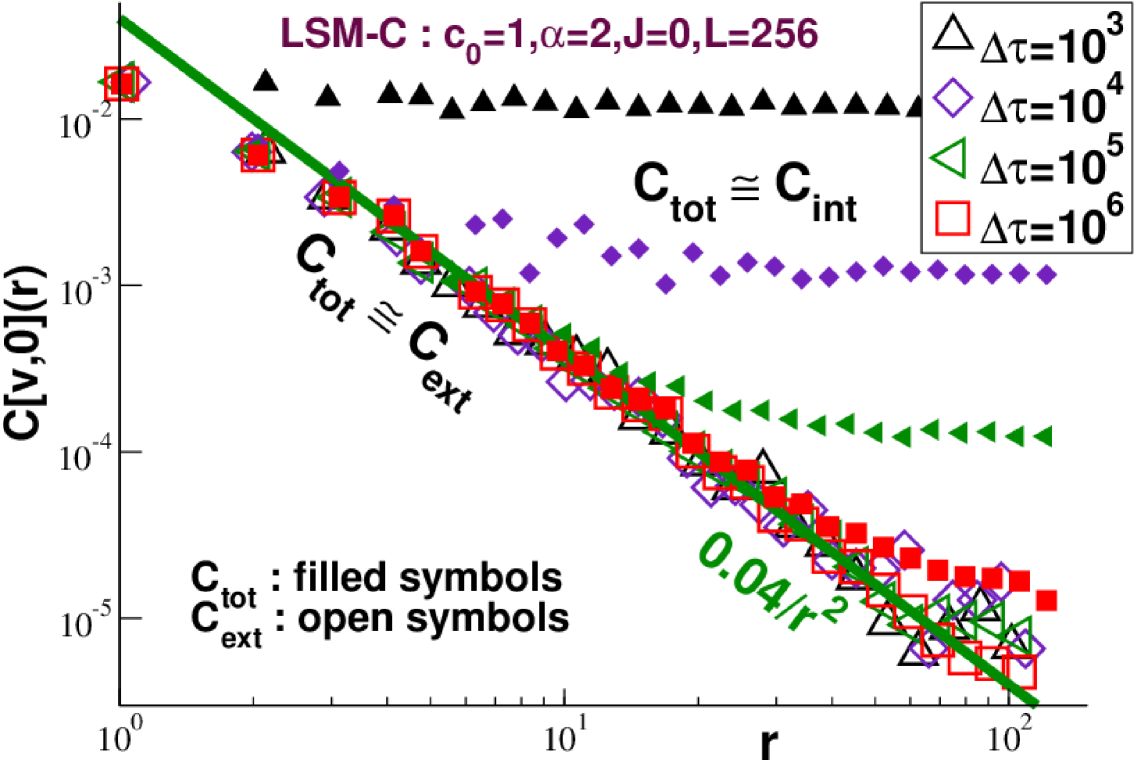
Figure 13: Isotropic projections $C_{\mathrm{tot}}[v](r,\Delta\tau)$ and $C_{\mathrm{ext}}[v](r,\Delta\tau)$ for LSM-C with $\alpha=2$, $J=0$ and $L=256$. Also indicated is the imposed asymptotic limit $C[b](r)\approx 0.04/r^{2}$ (bold solid line) for large $\Delta\tau$ and $V$ for both correlation functions. While $C_{\mathrm{ext}}[v](r,\Delta\tau)\approx C[b](r)$ for $\Delta\tau\gg\tau_{\mathrm{b}}$, $C_{\mathrm{tot}}[v](r,\Delta\tau)$ is seen to converge much more slowly to the large-$\Delta\tau$ limit.

The scaling of $C_{\mathrm{ext}}[v](r,\Delta\tau)$ and $C_{\mathrm{tot}}[v](r,\Delta\tau)$ with $\Delta\tau$ is illustrated in Fig. 13. We present here data obtained for LSM-C with $\alpha=2$, $J=0$ and $L=256$. Importantly, both $C_{\mathrm{tot}}[v](r,\Delta\tau)$ and $C_{\mathrm{ext}}[v](r,\Delta\tau)$ must approach for sufficiently large $\Delta\tau$ the (known) asymptotic limit $C[b](r)\approx 0.04/r^{2}$ (bold solid line) imposed by construction. $N_{\mathrm{k}}=1000$ is used for $\Delta\tau\leq 10^{3}$ to improve the precision of the $N_{\mathrm{k}}$-extrapolation for the external correlation function. While $C_{\mathrm{ext}}[v](r,\Delta\tau)$ becomes rapidly $\Delta\tau$-independent ($\Delta\tau\gg\tau_{\mathrm{b}}$) several orders of magnitude larger sampling times are needed for $C_{\mathrm{tot}}[v](r,\Delta\tau)$. This is caused by the internal contribution $C_{\mathrm{int}}[v](r,\Delta\tau)\propto 1/\Delta\tau$ to the total correlation function. This is also responsible for the leveling-off of $C_{\mathrm{tot}}[v](r,\Delta\tau)$ for large $r\gg r_{\mathrm{ne}}(\Delta\tau)$ with $r_{\mathrm{ne}}(\Delta\tau)$ being a crossover distance defined by $C_{\mathrm{int}}[v](r_{\mathrm{ne}},\Delta\tau)=C_{\mathrm{ext}}[v](r_{\mathrm{ne}})$. For the same reasons that $\delta v_{\mathrm{tot}}(\Delta\tau,V)$ is problematic for the determination of the system-size exponent $\gamma$, only computing $C_{\mathrm{tot}}[v](r,\Delta\tau)$ for one $\Delta\tau$ may incorrectly suggest a weak (possibly long-ranged) decay of the correlations. Only the $r$-regime where the data sets for the largest available $\Delta\tau$ clearly collapse can be used. This would be in the presented case less than an order of magnitude. Similar behavior has been found for all LSM versions.

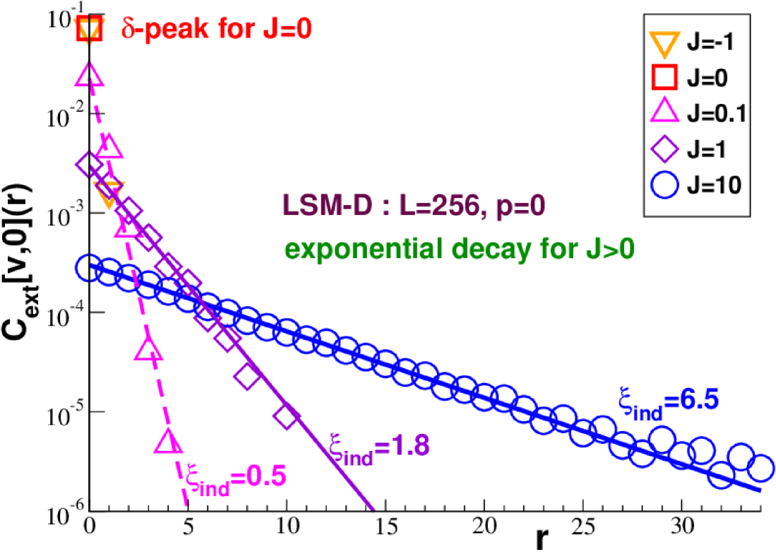
Figure 14: Isotropic projection $C_{\mathrm{ext}}[v,0](r,\Delta\tau)$ for LSM-D for different $J$. A $\delta(r)$-peak is observed for $J=0$ while $C_{\mathrm{ext}}[v,0](r,\Delta\tau)\propto\exp(-r/\xi_{\mathrm{ind}}(J))$ for $J>0$.

As a last example we come back to LSM-D and present the isotropic ($p=0$) external correlations $C_{\mathrm{ext}}[v,0](r)$ for different $J$ obtained for $\Delta\tau\gg\tau_{\mathrm{b}}(J)$. This is shown in Fig. 14 using half-logarithmic coordinates. As expected from the imposed (quenched) anisotropic $a$- and $b$-fields of the LSM-D (Table 1) a $\delta(r)$-peak at the origin is observed if all spring interactions are switched off ($J=0$). At variance with this the external correlation functions decay exponentially for $J>0$. Apparently, the corresponding induced correlation length $\xi_{\mathrm{ind}}(J)$ increases with $J$ but remains finite. The range of the correlations thus increases but stays short-ranged in agreement with the exponent $\gamma=1/2$ seen in Fig. 8.

6 Conclusion

6.1 General points made

Extending recent work on stochastic processes in non-ergodic macroscopic systems spmP1 ; spmP2 ; spmP3 we have investigated the different types of spatial correlation functions $C({\bf r})$ related to the macroscopic variances $\delta{\cal O}^{2}$ of observables ${\cal O}[\mathbf{x}]$ of time-series $\mathbf{x}$. As reminded in Sec. 4 the standard total variance $\delta{\cal O}^{2}_{\mathrm{tot}}(\Delta\tau)$ is the sum of an internal variance $\delta{\cal O}^{2}_{\mathrm{int}}(\Delta\tau)$ and an external variance $\delta{\cal O}^{2}_{\mathrm{ext}}(\Delta\tau)$, cf. Eq. (1). While $\delta{\cal O}_{\mathrm{int}}(\Delta\tau)\simeq 1/\sqrt{\Delta\tau}$ for $\Delta\tau\gg\tau_{\mathrm{b}}$, $\delta{\cal O}_{\mathrm{ext}}(\Delta\tau,V)\simeq\Delta_{\mathrm{ne}}(V)$ becomes constant. One motivation of this work (cf. Sec. 1.2) was to understand the $V$-dependence of the non-ergodicity parameter $\Delta_{\mathrm{ne}}$ in systems with (possibly long-ranged) spatial correlations. The generally important novel key results of this study were presented in Sec. 5 and Appendix A. As shown there, assuming ${\cal O}[\mathbf{x}]$ to be a spatial average of a local field ${\cal O}_{{\bf r}}$, the three global variances can be written as volume averages of the three spatial correlation functions $C_{\mathrm{tot}}({\bf r})$, $C_{\mathrm{int}}({\bf r})$ and $C_{\mathrm{ext}}({\bf r})$ and, moreover, $C_{\mathrm{tot}}({\bf r})=C_{\mathrm{int}}({\bf r})+C_{\mathrm{ext}}({\bf r})$ holds. The $\Delta\tau$- and $V$-dependences of the global variances can thus be traced back to the internal and external correlation functions $C_{\mathrm{int}}({\bf r})$ and $C_{\mathrm{ext}}({\bf r})$.

6.2 Specific fields considered

Focusing on the arithmetic mean ${\cal O}[\mathbf{x}]=m[\mathbf{x}]=\mathbf{E}^{t}x_{t}$ and especially on the empirical variance ${\cal O}[\mathbf{x}]=v[\mathbf{x}]=\mathbf{V}^{t}x_{t}$ of time-series (cf. Sec. 3) we illustrated the various general theoretical relations by means of MC simulations of variants of a simple lattice spring model (LSM) in two dimensions characterized by two quenched and spatial correlated fields (Table 1). We have especially investigated $\delta v_{\mathrm{int}}(\Delta\tau,V)$ and $\delta v_{\mathrm{ext}}(\Delta\tau,V)$ and the corresponding correlation functions $C_{\mathrm{int}}[v]({\bf r},\Delta\tau,V)$ and $C_{\mathrm{ext}}[v]({\bf r},\Delta\tau,V)$. As discussed in Sec. 5.2 and Appendix B, under general assumptions the internal correlation function is given by Eq. (57), i.e. it decreases inversely with $\Delta\tau$ for $\Delta\tau\gg\tau_{\mathrm{b}}$ and becomes constant, $C_{\mathrm{int}}[v]({\bf r},\Delta\tau,V)\simeq\delta v^{2}_{\mathrm{int}}(\Delta\tau)/2$, for large $r$ (cf. Fig. 12) albeit the primary instantaneous field $x_{t{\bf r}}$ is decorrelated. The external correlation function becomes $\Delta\tau$-independent for $\Delta\tau\gg\tau_{\mathrm{b}}$ (cf. Fig. 13). The last statement requires a proper $N_{\mathrm{k}}$-extrapolation by means of Eq. (53) or that the data are sampled using sufficiently large $\Delta\tau$ and $N_{\mathrm{k}}$, i.e. the correction term $C_{\mathrm{int}}[v]({\bf r},\Delta\tau,V)/N_{\mathrm{k}}$ in Eq. (53) must be negligible. Importantly, $C_{\mathrm{int}}[v]({\bf r},\Delta\tau)\gg C_{\mathrm{ext}}[v]({\bf r})$ for small $\Delta\tau$, large $V$ and large $r$. In these limits and due to large crossover effects $C_{\mathrm{tot}}[v]({\bf r},\Delta\tau)$ may deviate from its large-$\Delta\tau$ limit $C_{\mathrm{ext}}[v]({\bf r})$. Importantly, this may lead to an overestimation of the range of correlations as shown in Fig. 13.

6.3 Outlook

Some of the presented relations and technical features will be used in a presentation currently under preparation focusing on shear stresses $x_{t}=\sigma_{t}$ and associated shear-stress fields $x_{t{\bf r}}=\sigma_{t{\bf r}}$ Lemaitre14 ; Lemaitre15 . Again focusing on $\Delta\tau\gg\tau_{\mathrm{b}}$ we investigate $C_{\mathrm{int}}[f]({\bf r})$ and $C_{\mathrm{ext}}[f]({\bf r})$ for $f=m$ and $f=v$ for a broad range of particle numbers $n\approx V$. As central results it will be shown that $C_{\mathrm{ext}}[f]({\bf r})$ is long-ranged for both $f=m$ and $f=v$ decreasing as a power law $1/r^{\alpha}$ with $\alpha\approx d$. While the scaling of $C_{\mathrm{ext}}[m]({\bf r})$ is expected from previous simulations Lemaitre14 ; Lemaitre15 and recent theoretical work Fuchs17 ; Fuchs18 ; Fuchs19 ; lyuda18 the long-range decay of $C_{\mathrm{ext}}[v]({\bf r})$ is non-trivial and, as we shall discuss, indicates that the corresponding local elastic field is also long-ranged.

Author contribution statement

JPW designed and wrote the project benefiting from contributions of all authors.

Data availability statement

It was not possible to store all the $N_{\mathrm{c}}\times N_{\mathrm{k}}\times N_{\mathrm{t}}\times L^{2}$ primary fields $x_{ckt{\bf q}}$ which were immediately deleted after having been analyzed. Tables of the global averages have been kept, however, for a broad range of $\Delta\tau$ and $V$ and different LSM variants. These data sets are available from the corresponding author on reasonable request.

Appendix A Spatial correlations of periodic microcells

A.1 Some useful general relations

Let us begin by stating several useful general relations for spatial correlation functions of $d$-dimensional, real, discrete and periodic fields. As defined by Eq. (13) or Eq. (14) we consider the instantaneous correlation function $K[y_{{\bf r}}]({\bf r})$ of a field $y_{{\bf r}}$ of volume average $y\equiv\mathbf{E}^{{\bf r}}y_{{\bf r}}$. Obviously,

$$K[y_{{\bf r}}-y]({\bf r})=K[y_{{\bf r}}]({\bf r})-y^{2}.$$ (58)

Let us assume that the field $y_{l{\bf r}}$ additionally depends on an index $l$. We use below the averages $y_{l}=\mathbf{E}^{{\bf r}}y_{l{\bf r}}$, $y_{{\bf r}}=\mathbf{E}^{l}y_{l{\bf r}}$ and $y=\mathbf{E}^{l}y_{l}=\mathbf{E}^{{\bf r}}y_{{\bf r}}$. Rewriting Eq. (58) and summing over $l$ gives

$$\mathbf{E}^{l}K[y_{l{\bf r}}-y_{l}]({\bf r})=\mathbf{E}^{l}K[y_{l{\bf r}}]({\bf r})-\mathbf{E}^{l}y_{l}^{2}.$$ (59)

Also it is seen by expansion using Eq. (13) that

$$\mathbf{E}^{l}K[y_{l{\bf r}}-\lambda y_{{\bf r}}]({\bf r})=\mathbf{E}^{l}K[y_{l{\bf r}}]({\bf r})-\lambda(2-\lambda)K[y_{{\bf r}}]({\bf r})$$ (60)

for any real constant $\lambda$.

We remind that $\mathbf{V}^{l}y_{l}=\mathbf{E}^{l}y_{l}^{2}-y^{2}=\mathbf{E}^{l}(y_{l}-y)^{2}$. Using again Eq. (58) and the periodicity of the grid the variance $\mathbf{V}^{l}y_{l}$ may be written as the volume average

$$\mathbf{V}^{l}y_{l} = \mathbf{E}^{{\bf r}}C({\bf r})\mbox{ with }$$ (61)

$$C({\bf r}) \equiv \mathbf{E}^{l}K[y_{l{\bf r}}-y]({\bf r})\equiv\mathbf{E}^{l}K[y_{l{\bf r}}]({\bf r})-y^{2}$$ (62)

being the $l$-averaged correlation function in real space. By comparing Eq. (59) and Eq. (62) we may also write

$$C({\bf r})=\mathbf{E}^{l}K[y_{l{\bf r}}-y_{l}]({\bf r})+\mathbf{V}^{l}y_{l}$$ (63)

which using Eq. (61) implies $\mathbf{E}^{{\bf r}}\mathbf{E}^{l}K[y_{l{\bf r}}-y_{l}]({\bf r})=0$. It is useful to state two important limits for $C({\bf r})$: (i) At the origin we have

$$C({\bf r}={\bf 0})=\mathbf{V}^{l{\bf r}^{\prime}}y_{l{\bf r}^{\prime}}=\mathbf{E}^{l}\mathbf{V}^{{\bf r}^{\prime}}y_{l{\bf r}^{\prime}}+\mathbf{V}^{l}\mathbf{E}^{{\bf r}^{\prime}}y_{l{\bf r}^{\prime}}$$ (64)

and (ii) $C({\bf r})$ exactly vanishes if and only if

$$\mathbf{E}^{l}\mathbf{E}^{{\bf r}^{\prime}}y_{{\bf r}^{\prime}+{\bf r}}y_{{\bf r}^{\prime}}=\mathbf{E}^{l}\mathbf{E}^{{\bf r}^{\prime}}y_{{\bf r}^{\prime}+{\bf r}}\times\mathbf{E}^{l}\mathbf{E}^{{\bf r}^{\prime}}y_{{\bf r}^{\prime}}=y^{2}$$ (65)

as it happens for most (albeit not all) fields for sufficiently large $r=|{\bf r}|$. See Appendix B.1 for an exception relevant for the present study.

Moreover, with $z=\mathbf{E}^{{\bf r}}z_{{\bf r}}$ being an $l$-independent quantity it follows from Eq. (61) that

$$\mathbf{V}^{l}(y_{l}-z)=\mathbf{E}^{{\bf r}}\ \mathbf{E}^{l}K[(y_{l{\bf r}}-z_{{\bf r}})-(y-z)]({\bf r}).$$ (66)

Since $\mathbf{V}^{l}y_{l}=\mathbf{V}^{l}(y_{l}-z)$ this implies quite generally that

$$\mathbf{E}^{{\bf r}}\mathbf{E}^{l}K[\delta y_{l{\bf r}}]({\bf r})=\mathbf{E}^{{\bf r}}\mathbf{E}^{l}K[\delta y_{l{\bf r}}-\delta z_{{\bf r}}]({\bf r})$$ (67)

with $\delta y_{l{\bf r}}=y_{l{\bf r}}-y$ and $\delta z_{{\bf r}}=z_{{\bf r}}-z$, i.e. the correlation function of a field $y_{l{\bf r}}$ can be shifted by an $l$-independent field $z_{{\bf r}}$ without changing the $l$-averaged volume average.

A.2 Derivation of correlation functions

Using these general relations it is readily seen that the correlation functions defined as

$$C_{\mathrm{tot}}({\bf r}) \equiv \mathbf{E}^{l}K[{\cal O}_{l{\bf r}}-{\cal O}]({\bf r})=\mathbf{E}^{l}K[{\cal O}_{l{\bf r}}]({\bf r})-{\cal O}^{2}$$ (68)

$$C_{\mathrm{ext}}({\bf r}) \equiv \mathbf{E}^{c}K[{\cal O}_{c{\bf r}}-{\cal O}]({\bf r})=\mathbf{E}^{c}K[{\cal O}_{c{\bf r}}]({\bf r})-{\cal O}^{2}$$ (69)

$$C_{\mathrm{int}}({\bf r}) \equiv \mathbf{E}^{c}\mathbf{E}^{k}K[{\cal O}_{ck{\bf r}}-{\cal O}_{c{\bf r}}]({\bf r})$$ (70)

are consistent with Eqs. (3-6). The index $l$ runs again over all independent configurations $c$ and all time-series $k$ for each $c$ and the expectation value ${\cal O}$ is defined in Eq. (32). The corresponding equations in reciprocal space are given in Sec. 5.1, Eqs. (47-49). That Eq. (68) is consistent with $\delta{\cal O}^{2}_{\mathrm{tot}}=\mathbf{E}^{{\bf r}}C_{\mathrm{tot}}({\bf r})$ and Eq. (69) with $\delta{\cal O}^{2}_{\mathrm{ext}}=\mathbf{E}^{{\bf r}}C_{\mathrm{ext}}({\bf r})$ is directly implied by Eq. (61) and Eq. (62). To show that Eq. (70) is consistent with $\delta{\cal O}^{2}_{\mathrm{int}}=\mathbf{E}^{{\bf r}}C_{\mathrm{int}}({\bf r})$ and that all three correlation functions sum up according to Eq. (6) let us first note that due to Eq. (60) for $\lambda=1$ the internal correlation function may be rewritten as

$$C_{\mathrm{int}}({\bf r})=\mathbf{E}^{c}\left\{\mathbf{E}^{k}K[{\cal O}_{ck{\bf r}}]({\bf r})-K[{\cal O}_{c{\bf r}}]({\bf r})\right\}.$$ (71)

Using Eq. (68) and Eq. (69) this implies $C_{\mathrm{int}}({\bf r})=C_{\mathrm{tot}}({\bf r})-C_{\mathrm{ext}}({\bf r})$ in agreement with the key relation Eq. (6) stated in the Introduction. In turn we thus have

$$\mathbf{E}^{{\bf r}}C_{\mathrm{int}}({\bf r}) = \mathbf{E}^{{\bf r}}\left(C_{\mathrm{tot}}({\bf r})-C_{\mathrm{ext}}({\bf r})\right)$$ (72)

$$= \delta{\cal O}^{2}_{\mathrm{tot}}-\delta{\cal O}^{2}_{\mathrm{ext}}=\delta{\cal O}^{2}_{\mathrm{int}}$$

where we have used Eq. (1) in the last step.

Please note that due to Eq. (67) $\delta{\cal O}^{2}_{\mathrm{int}}=\mathbf{E}^{{\bf r}}C_{\mathrm{int}}({\bf r})$ would also be solved by the more general internal correlation function

$$C_{\mathrm{int}}({\bf r},\lambda)\equiv\mathbf{E}^{c}\mathbf{E}^{k}K[({\cal O}_{ck{\bf r}}-{\cal O}_{c})-\lambda({\cal O}_{c{\bf r}}-{\cal O}_{c})]({\bf r})$$ (73)

which reduces to Eq. (70) for $\lambda=1$, since it is possible to shift ${\cal O}_{ck{\bf r}}-{\cal O}_{c}$ with the $k$-independent field $\lambda({\cal O}_{c{\bf r}}-{\cal O}_{c})$ without changing the $k$-averaged volume average. The trouble with such alternative definitions is that Eq. (6) does not hold anymore in general, e.g., it can be shown that Eq. (73) leads to

$$C_{\mathrm{tot}}({\bf r})=C_{\mathrm{int}}({\bf r},\lambda)+\lambda(2-\lambda)C_{\mathrm{ext}}({\bf r})+(\lambda-1)^{2}\delta{\cal O}^{2}_{\mathrm{ext}}.$$ (74)

Due to the last term and since $\delta{\cal O}^{2}_{\mathrm{ext}}>0$ for non-ergodic systems all three correlation functions may in principle only vanish for the same ${\bf r}$ for $\lambda=1$ and for exactly this limit Eq. (74) reduces to Eq. (6). We therefore set $\lambda=1$.

A.3 Important limits

We have omitted for clarity in the preceding subsection all possible dependences on $N_{\mathrm{c}}$, $N_{\mathrm{k}}$, $\Delta\tau$ and $V$. However, it is assumed below that $N_{\mathrm{c}}$ and $N_{\mathrm{k}}$ are arbitrarily large, i.e. all properties are $N_{\mathrm{c}}$- and $N_{\mathrm{k}}$-independent. Moreover, we focus on the limit $\Delta\tau\gg\tau_{\mathrm{b}}$, i.e. both ${\cal O}_{c{\bf r}}=\mathbf{E}^{k}{\cal O}_{ck{\bf r}}$ and its average ${\cal O}=\mathbf{E}^{c}\mathbf{E}^{{\bf r}}{\cal O}_{c{\bf r}}$ are $\Delta\tau$-independent to leading order. Due to Eq. (69) the same holds for the external correlation function, i.e.

$$C_{\mathrm{ext}}({\bf r},\Delta\tau,V)\simeq C_{\mathrm{ext}}({\bf r},V)\mbox{ for }\Delta\tau\gg\tau_{\mathrm{b}}.$$ (75)

The indicated $V$-dependence drops out if ${\cal O}_{c{\bf r}}$ is $V$-independent as in all the models of this work.

The internal correlation function, Eq. (70), characterizes the correlations of the difference ${\cal O}_{ck{\bf r}}(\Delta\tau)-{\cal O}_{c{\bf r}}$. While ${\cal O}_{ck{\bf r}}(\Delta\tau)$ depends in general not only on $k$ but also on $\Delta\tau$, both dependences drop out for $\Delta\tau\to\infty$. Hence, ${\cal O}_{ck{\bf r}}(\Delta\tau)\to{\cal O}_{c{\bf r}}$ and in turn

$$\lim_{\Delta\tau\to\infty}C_{\mathrm{int}}({\bf r},\Delta\tau,V)=0.$$ (76)

To obtain the internal correlation function for finite $\Delta\tau\gg\tau_{\mathrm{b}}$ it should be remembered that ${\cal O}_{ck{\bf r}}(\Delta\tau)$ is a time-averaged moment over $N_{\mathrm{t}}=\Delta\tau/\delta\tau$ data entries from one stored time-series. The internal correlation function can thus be written as an average

$$C_{\mathrm{int}}({\bf r}={\bf r}_{2}-{\bf r}_{1},\Delta\tau,V)=\mathbf{E}^{c}\mathbf{E}^{{\bf r}_{1}}\left(\mathbf{E}^{t_{1}}\mathbf{E}^{t_{2}}\mathbf{E}^{k}\ldots\right)$$ (77)

over entries measured at discrete times $t_{1}$ and $t_{2}$. A specific example is worked out in Appendix B.1. If one assumes for simplicity that $\delta\tau\gg\tau_{\mathrm{b}}$ only contributions with $t_{1}=t_{2}$ can contribute. Using also that the time-average $\mathbf{E}^{t}$ is normalized by $N_{\mathrm{t}}\propto\Delta\tau$, this shows that quite generally the internal correlation function must decay to leading order for all ${\bf r}$ as

$$C_{\mathrm{int}}({\bf r},\Delta\tau,V)\propto\frac{1}{\Delta\tau}\mbox{ for }\Delta\tau\gg\tau_{\mathrm{b}}$$ (78)

as expected from $\delta{\cal O}^{2}_{\mathrm{int}}(\Delta\tau)=\mathbf{E}^{{\bf r}}C_{\mathrm{int}}({\bf r})\propto 1/\Delta\tau$.

Appendix B Scaling of $C_{\mathrm{int}}[v]({\bf r},\Delta\tau,V)$

B.1 Predictions for LSM-A

case	$\mathbf{E}^{k}A_{1}A_{2}$	$\mathbf{E}^{k}A_{1}B_{2}$	$\mathbf{E}^{k}A_{2}B_{1}$	$\mathbf{E}^{k}B_{1}B_{2}$
1. ${\bf r}_{1}={\bf r}_{2}={\bf r}_{3}={\bf r}_{4}$	$2b_{c{\bf r}_{1}}^{2}/N_{\mathrm{t}}$	$3b_{c{\bf r}_{1}}^{2}/N_{\mathrm{t}}^{2}$	$3b_{c{\bf r}_{1}}^{2}/N_{\mathrm{t}}^{2}$	$b_{c{\bf r}_{1}}^{2}/N_{\mathrm{t}}^{3}$
2. ${\bf r}_{1}={\bf r}_{2}\neq{\bf r}_{3}={\bf r}_{4}$	$b_{c{\bf r}_{1}}(\mathbf{S}^{{\bf r}_{3}\neq{\bf r}_{1}}b_{c{\bf r}_{3}})/N_{\mathrm{t}}$	$b_{c{\bf r}_{1}}^{2}(V-1)/N_{\mathrm{t}}^{2}$	$b_{c{\bf r}_{1}}^{2}(V-1)/N_{\mathrm{t}}^{2}$	$b_{c{\bf r}_{1}}^{2}(V-1)/N_{\mathrm{t}}^{2}$
3. ${\bf r}_{1}={\bf r}_{3}\neq{\bf r}_{2}={\bf r}_{4}$	0	0	0	$b_{c{\bf r}_{1}}b_{c{\bf r}_{2}}/N_{\mathrm{t}}^{2}$
4. ${\bf r}_{1}={\bf r}_{4}\neq{\bf r}_{2}={\bf r}_{3}$	$b_{c{\bf r}_{1}}b_{c{\bf r}_{2}}/N_{\mathrm{t}}$	$b_{c{\bf r}_{1}}b_{c{\bf r}_{2}}/N_{\mathrm{t}}^{2}$	$b_{c{\bf r}_{1}}b_{c{\bf r}_{2}}/N_{\mathrm{t}}^{2}$	$b_{c{\bf r}_{1}}b_{c{\bf r}_{2}}/N_{\mathrm{t}}^{2}$

Table 2: $k$-averages $\mathbf{E}^{k}A_{1}A_{2}$, $\mathbf{E}^{k}A_{1}B_{2}$, $\mathbf{E}^{k}A_{2}B_{1}$ and $\mathbf{E}^{k}B_{1}B_{2}$ for LSM-A. The different relevant cases for ${\bf r}_{1}$, ${\bf r}_{2}$, ${\bf r}_{3}$, ${\bf r}_{4}$ are indicated in the first column. Note that $r=|{\bf r}|$ with ${\bf r}={\bf r}_{2}-{\bf r}_{1}$. The first two cases indicate contributions for $r=0$, the last two cases contributions for $r>0$. $\mathbf{E}^{k}A_{1}B_{2}$ and $\mathbf{E}^{k}A_{2}B_{1}$ are identical by symmetry. The leading contributions of order ${\cal O}(\Delta\tau^{-1})$ are due to $\mathbf{E}^{k}A_{1}A_{2}$ (second column). The second case (${\bf r}_{1}={\bf r}_{2}\neq{\bf r}_{3}={\bf r}_{4}$) yields contributions proportional to the system size.

As noted in Appendix A.1, all correlation functions $C[f]({\bf r})$ discussed in the present work must vanish if Eq. (65) holds, i.e. if two typical points of the field $f$ at a respective distance ${\bf r}$ are uncorrelated. Here we draw attention to the fact that although the primary instantaneous field $x_{t{\bf r}}$ may be uncorrelated this may not be the case for the field ${\cal O}_{{\bf r}}$ associated to the time-averaged functional ${\cal O}[\mathbf{x}]$ of the time-series $\mathbf{x}$. As we shall see, this matters specifically for the covariance field, Eq. (30),

$$v_{ck{\bf r}} = V\left\{\mathbf{E}^{t}x_{ckt{\bf r}}x_{ckt}-x_{ck{\bf r}}x_{ck}\right\}$$ (79)

$$= \mathbf{S}^{{\bf r}^{\prime}}\left\{\mathbf{E}^{t}x_{ckt{\bf r}}x_{ckt{\bf r}^{\prime}}-\mathbf{E}^{t}\mathbf{E}^{t^{\prime}}x_{ckt{\bf r}}x_{ckt^{\prime}{\bf r}^{\prime}}\right\}$$

restated for convenience omitting the irrelevant prefactor $\beta$ and introducing the sum $\mathbf{S}^{{\bf r}^{\prime}}\equiv V\mathbf{E}^{{\bf r}^{\prime}}$. In the second step we have made explicit the crucial contributions with ${\bf r}^{\prime}\neq{\bf r}$ to the averages $x_{ckt}$ and $x_{ck}$.

Without restricting the generality of the argument let us focus on the model LSM-A with $J=0$, i.e. the $x_{ckt{\bf r}}$ of different microcells ${\bf r}$ are uncorrelated. Ultimately, we want to expand $v_{ck{\bf r}}$ for large $\Delta\tau$. Reminding Eq. (31) it is thus useful that the $x_{ckt{\bf r}}$ in Eq. (79) can be replaced by $\delta x_{ckt{\bf r}}\equiv x_{ckt{\bf r}}-a_{c{\bf r}}$ without changing $v_{ck{\bf r}}$. Moreover, let us assume that the data is sampled with large time increments $\delta\tau\gg\tau_{\mathrm{b}}$, i.e. different times $t^{\prime}$ and $t^{\prime\prime}$ can be considered to be uncorrelated. This implies that

$$\mathbf{E}^{k}\delta x_{ckt^{\prime}{\bf r}^{\prime}}^{p^{\prime}}\delta x_{ckt^{\prime\prime}{\bf r}^{\prime\prime}}^{p^{\prime\prime}}=\mathbf{E}^{k}\delta x_{ckt^{\prime}{\bf r}^{\prime}}^{p^{\prime}}\mathbf{E}^{k}\delta x_{ckt^{\prime\prime}{\bf r}^{\prime\prime}}^{p^{\prime\prime}}$$ (80)

whenever $t^{\prime}\neq t^{\prime\prime}$ or ${\bf r}^{\prime}\neq{\bf r}^{\prime\prime}$ ($p^{\prime}$ and $p^{\prime\prime}$ being integers) and, moreover, the following useful relations hold:

$$\mathbf{E}^{t}\mathbf{E}^{t^{\prime}}\delta_{tt^{\prime}} = 1/N_{\mathrm{t}},$$ (81)

$$\mathbf{E}^{k}\delta x_{ckt{\bf r}} = 0,$$ (82)

$$\mathbf{E}^{k}\delta x_{ckt{\bf r}}\delta x_{ckt^{\prime}{\bf r}^{\prime}} = b_{c{\bf r}}\ \delta_{{\bf r}{\bf r}^{\prime}}\delta_{tt^{\prime}},$$ (83)

$$\mathbf{E}^{k}\delta x_{ckt{\bf r}}^{2}\delta x_{ckt{\bf r}^{\prime}}^{2} = 3b_{c{\bf r}}^{2}\ \delta_{{\bf r}{\bf r}^{\prime}}+b_{c{\bf r}}b_{c{\bf r}^{\prime}}(1-\delta_{{\bf r}{\bf r}^{\prime}}).$$ (84)

We have used above that the lattice springs are Gaussian variables, Eq. (12), i.e. for each independent spring of length $x_{c{\bf r}}$ (dropping the indices $k$ and $t$) we have $\left<\delta x_{c{\bf r}}\right>=0$, $\left<\delta x_{c{\bf r}}^{2}\right>=b_{c{\bf r}}$ and $\left<\delta x_{c{\bf r}}^{4}\right>=3b_{c{\bf r}}^{2}$ with $\left<\ldots\right>$ denoting the thermal average within each basin $c$. Using Eqs. (81-83) we obtain, e.g., the $k$-average

$$v_{c{\bf r}}=\mathbf{E}^{k}v_{ck{\bf r}}=b_{c{\bf r}}\left(1-1/N_{\mathrm{t}}\right)$$ (85)

and, hence, the total average $v=\mathbf{E}^{c}\mathbf{E}^{{\bf r}}v_{c{\bf r}}=b(1-1/N_{\mathrm{t}})$ with $b=\mathbf{E}^{c}\mathbf{E}^{{\bf r}}b_{c{\bf r}}$.

To compute the internal correlation function we write

$$C_{\mathrm{int}}[v]({\bf r}) = \mathbf{E}^{c}C_{c}({\bf r})\mbox{ with }$$ (86)

$$C_{c}({\bf r}) = \mathbf{E}^{k}K[(v_{ck{\bf r}}-b_{c{\bf r}})-(v_{c{\bf r}}-b_{c{\bf r}})]({\bf r})$$ (87)

$$= \mathbf{E}^{k}K[v_{ck{\bf r}}-b_{c{\bf r}}]({\bf r})-K[v_{c{\bf r}}-b_{c{\bf r}}]({\bf r})$$ (88)

using Eq. (71) in the last step. Due to Eq. (85) it is clear that the second term in Eq. (88) is of order ${\cal O}(\Delta\tau^{-2})$ We can focus on the first term which we rewrite as volume average $\mathbf{E}^{{\bf r}_{1}}\tilde{C}_{c}({\bf r}_{1},{\bf r}_{2}={\bf r}_{1}+{\bf r})$ with

$$\tilde{C}_{c{\bf r}_{1}{\bf r}_{2}}({\bf r}_{1},{\bf r}_{2}) \equiv \mathbf{E}^{k}(v_{ck{\bf r}_{1}}-b_{c{\bf r}_{1}})(v_{ck{\bf r}_{2}}-b_{c{\bf r}_{2}})$$ (89)

$$= \mathbf{E}^{k}(A_{1}-B_{1})(A_{2}-B_{2})$$ (90)

where Eq. (79) is used for the definition of the terms

$$A_{1} = \mathbf{S}^{{\bf r}_{3}}\mathbf{E}^{t_{1}}\left(\delta x_{ckt_{1}{\bf r}_{1}}\delta x_{ckt_{1}{\bf r}_{3}}-b_{c{\bf r}_{1}}\delta_{{\bf r}_{1}{\bf r}_{3}}\right),$$ (91)

$$A_{2} = \mathbf{S}^{{\bf r}_{4}}\mathbf{E}^{t_{2}}\left(\delta x_{ckt_{2}{\bf r}_{2}}\delta x_{ckt_{2}{\bf r}_{4}}-b_{c{\bf r}_{2}}\delta_{{\bf r}_{2}{\bf r}_{4}}\right),$$ (92)

$$B_{1} = \mathbf{S}^{{\bf r}_{3}}\mathbf{E}^{t_{1}}\mathbf{E}^{t_{3}}\delta x_{ckt_{1}{\bf r}_{1}}\delta x_{ckt_{3}{\bf r}_{3}}\ \mbox{and}$$ (93)

$$B_{2} = \mathbf{S}^{{\bf r}_{4}}\mathbf{E}^{t_{2}}\mathbf{E}^{t_{4}}\delta x_{ckt_{2}{\bf r}_{2}}\delta x_{ckt_{4}{\bf r}_{4}}.$$ (94)

We expand the different contributions and $k$-average using the identities Eqs. (80-84). As summarized in Table 2 it is helpful to distinguish four cases for ${\bf r}_{1}$, ${\bf r}_{2}$, ${\bf r}_{3}$ and ${\bf r}_{4}$. Most contributions are of order ${\cal O}(\Delta\tau^{-2})$ and only three contributions of $\mathbf{E}^{k}A_{1}A_{2}$ (second column) do matter. A central result is that due to the last case (${\bf r}_{1}={\bf r}_{4}\neq{\bf r}_{2}={\bf r}_{3}$), the internal correlation function must remain finite for $r>0$. Note also that all terms for the second case (${\bf r}_{1}={\bf r}_{2}\neq{\bf r}_{3}={\bf r}_{4}$) increase linearly with $V$ due to the sum $\mathbf{S}^{{\bf r}_{3}}\mathbf{S}^{{\bf r}_{4}}\delta_{{\bf r}_{3}{\bf r}_{4}}(1-\delta_{{\bf r}_{1}{\bf r}_{3}})$. In fact, using $b_{c}=\mathbf{E}^{{\bf r}_{3}}b_{c{\bf r}_{3}}$, the indicated term for $\mathbf{E}^{k}A_{1}A_{2}$ can be rewritten as

$$b_{c{\bf r}_{1}}(\mathbf{S}^{{\bf r}_{3}\neq{\bf r}_{1}}b_{c{\bf r}_{3}})/N_{\mathrm{t}}=b_{c{\bf r}_{1}}b_{c}V/N_{\mathrm{t}}-b_{c{\bf r}_{1}}^{2}/N_{\mathrm{t}}.$$ (95)

We finally average over ${\bf r}_{1}$ and $c$ using that the $b_{c{\bf r}^{\prime}}$ are decorrelated for different ${\bf r}^{\prime}$. Summarizing all terms we obtain to leading order

$$C_{\mathrm{int}}[v]({\bf r})\simeq\frac{b^{2}}{N_{\mathrm{t}}}\times\left\{\begin{array}[]{ll}V+1&\mbox{ for }r=0,\\ 1&\mbox{ for }r>0.\end{array}\right.$$ (96)

As a consequence $\delta v^{2}_{\mathrm{int}}(\Delta\tau,V)=\mathbf{E}^{{\bf r}}C_{\mathrm{int}}[v]({\bf r})=2b^{2}/N_{\mathrm{t}}\propto V^{0}/\Delta\tau$, as expected.

B.2 Scaling for general Gaussian fields

It is clear that the above result can be generalized to other models with short-range correlations and general $\delta\tau$ including $\delta\tau\ll\tau_{\mathrm{b}}$. This merely requires a renormalization of space and time. Especially this suggests to replace $1/N_{\mathrm{t}}$ by $\delta v^{2}_{\mathrm{int}}(\Delta\tau)$. It is in this context of relevance that the above result Eq. (96) can be recast as

$$C_{\mathrm{int}}[v]({\bf r})\simeq\left\{V(1-\alpha)c({\bf r})+\alpha\right\}\delta v^{2}_{\mathrm{int}}(\Delta\tau)$$ (97)

with $\mathbf{S}^{{\bf r}}c({\bf r})=1$, $c({\bf r})\to 0$ for large $r$ (with $r\neq 0$ for LSM-A) and $\alpha=1/2$. Note that $\mathbf{E}^{{\bf r}}C_{\mathrm{int}}[v]({\bf r})=\delta v^{2}_{\mathrm{int}}(\Delta\tau)$ holds for all coefficients $\alpha$. As discussed in Sec. 5.2, the numerical results of all our LSM variants are consistent with this generalization of the direct calculation for the simple LSM-A model. (As far as we can tell this even holds reasonably for systems with long-range correlations.) There is in fact a general reason for expecting Eq. (97) to hold for many models: For a given $c$ the $x_{t{\bf r}}$-fluctuations are often nearly Gaussian. [For the LSM variants the joint distributions of the $x_{t{\bf r}}$ are in fact exactly Gaussian since the total energy is quadratic in $x_{t{\bf r}}$, Eq. (12).] This allows for a theoretical treatment of $C_{\mathrm{int}}[v]({\bf r})$ based on the cumulant formalism (“Wick’s theorem”) similar to the calculation which leads to Eq. (45) for the global variance $\delta v^{2}_{\mathrm{int}}(\Delta\tau)$ lyuda18 ; spmP1 . It is thus possible to show that Eq. (97) must hold for general fluctuating Gaussian fields with $\alpha=1/2$. This calculation is beyond of the scope of the present work.

References

- (1) L. Klochko, J. Baschnagel, J.P. Wittmer, A.N. Semenov, J. Chem. Phys. 151, 054504 (2019)
- (2) G. George, L. Klochko, A. Semenov, J. Baschnagel, J.P. Wittmer, EPJE 44, 13 (2021)
- (3) G. George, L. Klochko, A.N. Semenov, J. Baschnagel, J.P. Wittmer, EPJE 44, 54 (2021)
- (4) G. George, L. Klochko, A.N. Semenov, J. Baschnagel, J.P. Wittmer, EPJE 44, 125 (2021)
- (5) W. Götze, Complex Dynamics of Glass-Forming Liquids: A Mode-Coupling Theory (Oxford University Press, Oxford, 2009)
- (6) A. Heuer, J.Phys.: Condens. Matter 20, 373101 (2008)
- (7) I. Procaccia, C. Rainone, C.A.B.Z. Shor, M. Singh, Phys. Rev. E 93, 063003 (2016)
- (8) J.F. Lutsko, J. Appl. Phys 64, 1152 (1988)
- (9) J.F. Lutsko, J. Appl. Phys 65, 2991 (1989)
- (10) J.L. Barrat, Microscopic Elasticity of Complex Systems, in Computer Simulations in Condensed Matter Systems: From Materials to Chemical Biology - Vol. 2, edited by M. Ferrario, G. Ciccotti, K. Binder (Springer, Berlin and Heidelberg, 2006), Vol. 704, pp. 287—307
- (11) J.P. Wittmer, H. Xu, P. Polińska, F. Weysser, J. Baschnagel, J. Chem. Phys. 138, 12A533 (2013)
- (12) A. Lemaître, Phys. Rev. Lett. 113, 245702 (2014)
- (13) A. Lemaître, J. Chem. Phys. 143, 164515 (2015)
- (14) D.P. Landau, K. Binder, A Guide to Monte Carlo Simulations in Statistical Physics (Cambridge University Press, Cambridge, 2000)
- (15) W. Press, S. Teukolsky, W. Vetterling, B. Flannery, Numerical Recipes in FORTRAN: the art of scientific computing (Cambridge University Press, Cambridge, 1992)
- (16) M.P. Allen, D.J. Tildesley, Computer Simulation of Liquids, 2nd Edition (Oxford University Press, Oxford, 2017)
- (17) A.L. Barbabási, H. Stanley, Fractal Concepts in Surface Growth (Cambridge University Press, Cambridge, 1995)
- (18) M. Maier, A. Zippelius, M. Fuchs, Phys. Rev. Lett. 119, 265701 (2017)
- (19) M. Maier, A. Zippelius, M. Fuchs, J. Chem. Phys. 149, 084502 (2018)
- (20) F. Vogel, A. Zippelius, M. Fuchs, Europhys. Lett. 125, 68003 (2019)
- (21) L. Klochko, J. Baschnagel, J.P. Wittmer, A.N. Semenov, Soft Matter 14, 6835 (2018)
- (22) J.L. Lebowitz, J.K. Percus, L. Verlet, Phys. Rev. 153, 250 (1967)
- (23) J.P. Hansen, I.R. McDonald, Theory of simple liquids (Academic Press, New York, 2006), 3nd edition