Sequence Prediction Under Missing Data : An RNN Approach Without Imputation

Abstract.

Missing data scenarios are very common in ML applications in general and time-series/sequence applications are no exceptions. This paper pertains to a novel Recurrent Neural Network (RNN) based solution for sequence prediction under missing data. Our method is distinct from all existing approaches. It tries to encode the missingness patterns in the data directly without trying to impute data either before or during model building. Our encoding is lossless and achieves compression. It can be employed for both sequence classification and forecasting. We focus on forecasting here in a general context of multi-step prediction in presence of possible exogenous inputs. In particular, we propose novel variants of Encoder-Decoder (Seq2Seq) RNNs for this. The encoder here adopts the above mentioned pattern encoding, while at the decoder which has a different structure, multiple variants are feasible. We demonstrate the utility of our proposed architecture via multiple experiments on both single and multiple sequence (real) data-sets. We consider both scenarios where (i)data is naturally missing and (ii)data is synthetically masked.

1. Introduction

Sequence based prediction (classification (Xing et al., 2010) and forecasting (Lim and Zohren, 2021)), though an old research area continues to be very relevant given recent improvements and constant emergence of newer applications. RNNs are arguably one of the most popular state-of-art sequence predictive modeling approaches. Deep RNNs have achieved astounding success over the last decade in domains like NLP, speech and audio processing (van den Oord et al., 2016), computer vision (Wang and Tax, 2016), time series classification, forecasting and so on. In particular, it has achieved state-of-art performance (and beyond) in tasks like handwriting recognition (Graves et al., 2009), speech recognition (Graves et al., 2013; Graves and Jaitly, 2014), machine translation (Cho et al., 2014; Sutskever et al., 2014) and image captioning (Kiros et al., 2014; Xu et al., 2015), to name a few.

Sequence Prediction under missing data also has a long literature. Missing data could arise due to a variety of reasons like sensor malfunction, maintenance OR even high noise (noise level could be so high that considering data as missing would be more meaningful). Researchers have provided a variety of techniques for data imputation over the years (Johnson, 2013; Mondal and Percival, 2010; Koren et al., 2009; Rehfeld et al., 2011; García-Laencina et al., 2010), which is typically followed by the predictive modelling step. RNNs in particular have also been explored for sequence modelling under missing data over the years. This paper addresses sequence prediction under missing data using RNNs in a novel way. While our proposed ideas can be employed on both classification and forecasting, we focus on forecasting in this paper. In particular, we consider a general multi-step forecasting scenario with possibly additional exogenous inputs to be handled.

Encoder-Decoder (ED) OR Seq2Seq architecture used to map variable length sequences to another variable length sequence were first successfully applied for machine translation (Cho et al., 2014; Sutskever et al., 2014) tasks. From then on, the ED framework has been successfully applied in many other tasks like speech recognition(Lu et al., 2015), image captioning etc. Given its variable length Seq2Seq mapping ability, the ED framework has also been utilized for accurate multi-step (time-series) forecasting where the target vector length can be variable and independent of the input vector (Wen et al., 2017). The missing data RNN architecture proposed here for forecasting is essentially built on the basic ED architecture.

The forecasting task considered here involves predicting one or more endogenous variables over a multi-step forecast horizon in the presence of possible exogenous inputs which influence the evolution of the endogenous variables. Such forecasting tasks arise in diverse applications. A retailer may be interested in forecasting one or more products sales (modelled as endogenous variables) in the presence of exogenous price variation. In electricity markets, forecasting power demand (endogenous) in different geographical regions by factoring temperature influences/fluctuations (exogenous) is another example. We consider multi-step forecasting in such scenarios in the presence of missing data.

1.1. Contributions

The traditional approach for predictive modelling under missing data has been to impute first and then perform model learning of one’s choice. Accordingly, there have been a wide variety of data imputation techniques proposed in literature. However, this sequential approach of impute and model building is very sensitive to the quality of imputation. Also, the imputation step itself can be computationally intensive. To circumvent the above limitations of this approach, researchers have proposed approaches where imputation and model learning are carried out jointly. Among RNN based missing data works, many approaches follow the jointly impute and learn approach (Bengio and Gingras, 1995; Che et al., 2018).

Our proposed method in this paper adopts a fundamentally different (or distinct) approach compared to the above two broad class of approaches. We try to avoid imputation almost completely either before OR during model building. Our approach performs predictive model building by directly trying to learn the missingness patterns observed in the data. This novel general approach can be particularly useful in scenarios where the sequential data is missing in large consecutive chunks. In such scenarios, the existing impute based approaches will tend to suffer significant imputation errors.

Our contribution involves a novel ED architecture using two encoders, while allowing for intelligent choices/variants in the decoder which incorporates multi-step (target) learning. Overall contribution summary is as follows:

• We propose a novel encoding scheme of the input window without imputation, which is applicable for both sequence classification and forecasting. For multi-step forecasting in presence of exogenous inputs, we propose a novel ED based architecture which employs the above encoding scheme in the encoder.

• The missingness pattern in the input window of an example is encoded as it is (without imputation) using two encoders with variable length inputs. The encoding is lossless with significant compression feasible. The output window information can be translated into the decoder in multiple interesting ways.

• To utilize the proposed scheme for multiple sequence data, where per sequence data is less, we propose a heuristic procedure. We demonstrate effectiveness of our architecture variants on diverse real data sets.

2. Related work

Prediction under missing data is a classic problem with an old literature. One broad class of methods to address this is to first impute followed by predictive modeling. The simpler approaches towards data imputation include smoothing, interpolation, splines(Johnson, 2013) which capture straightforward patterns in the data. The more sophisticated approaches include spectral analysis (Mondal and Percival, 2010), matrix factorization (Koren et al., 2009), kernel methods (Rehfeld et al., 2011), EM algorithm (García-Laencina et al., 2010) etc. These sophisticated approaches can be computationally expensive. Imputation methods typically assume restricted scenarios like low missing rates, missing at random and so on which may not hold in practice. The two step sequential process of imputation followed by prediction can suffer from imputation errors while the predictive model so built is blind to any missingness pattern structure.

RNNs have been explored earlier for time-series tasks (sequence classification in particular) with missing data. The early RNN approaches have predominantly adopted a strategy of jointly imputing and model building. One of the first approaches based on non-gated RNNs seems to be in (Bengio and Gingras, 1995). The missing values here are initialized to an unconditional expected value and the RNN is unfolded in time for a few extra steps (allowed to relax) to allow the missing values to settle to something more reasonable while the other inputs are clamped to their observed values. The learning criterion is an output error minimization based on all time steps in the unfolded RNN. In (Tresp and Briegel, 1997), to mitigate errors while predicting in a free running OR teacher forcing mode, a linear correlated error model is assumed in addition to the NARX model. The overall learning scheme here involves a mix of Real-time Recurrent Learning for the nonlinear map and an EM algorithm for the error model. An RNN approach for speech recognition under missing data (on account of noise) was proposed in (Parveen and D. Green, 2001) which uses an adaption of the architecture in (Bengio and Gingras, 1995). In particular, (Bengio and Gingras, 1995) uses a Jordan network (Jordan, 1988) with feedback or recurrent connections from output to hidden units. In contrast, (Parveen and D. Green, 2001) avoided feedback from the output but instead considered recurrent connections from the hidden layer to the input and itself (with a unit-delay) on the lines of an Elman network (Elman, 1990).

Among the recent RNN approaches, (Lipton et al., 2016) considers diagnosis classification under (irregularly recorded) clinical time series. It learns missingness patterns without any explicit imputation. It encodes the missingness pattern with a simple additional binary vector (indicating presence or absence of data) as input while training. More recently, an approach GRU-D (Che et al., 2018) which incorporates both missingness pattern (as in (Lipton et al., 2016)) and the joint impute and learning strategy was proposed. Here, the missing data points are assumed to be a convex combination of the last observed value and the unconditional mean. The key intuition is that weight on the last observed value drops (decays) as the time point under consideration moves away from the last observed value (OR time delay). This decay factor is parameterized via a simple perceptron like nonlinear function of this time-delay whose weights are jointly learnt with the RNN (GRU) weights.

Among the recent RNN based forecasting approaches, (Cinar et al., 2018) proposes an attention-based encoder-decoder approach of imputing first either using padding (based on left end) OR interpolation (one can use any technique) and then learning by incorporating suitable re-weighting of the impact of these imputed values. This approach doesn’t handle exogenous inputs. The first missing data variant first imputes using padding from the left-end and considers learning another weight, which models the influence of these imputed values using an exponential decay based on the distance from the last available data point. The second variant uses interpolation (based on both left and right end values) to impute and then employs a re-weighting scheme using both the left and right end. It divides a gap into $3$ regions uniformly and learns a weight for each of these regions.

2.1. Proposed architecture in perspective

Our overall approach is to avoid the impute first to the extent possible. The proposed ED idea employs a unique approach of encoding the missingness pattern in the input window as it is without any imputation. Instead of using a single encoder with a binary encoding of the missingness pattern as in (Lipton et al., 2016), we employ two encoders resulting in a compressed and lossless encoding. This feature of our approach is very different from all existing approaches to the best of our knowledge.

Our novel idea of encoding the input window cannot be employed on the output window. This is because the decoder is unfolded exactly to the extent of forecast horizon and each time-step of the decoder is used to separately forecast for a particular future time-step. However, as we discuss later, one can encode the missing exogenous inputs using the binary encoding of (Lipton et al., 2016), which is one of our proposed variants on the decoder. A more powerful variant would be to employ the GRU-D approach on the decoder with exogenous future variables as inputs.

In summary, our approach incorporates useful aspects of (Lipton et al., 2016) and (Che et al., 2018) on the decoder, while it retains its unique distinguishing feature on the encoder side.

Compared to multi-step forecasting approach of (Cinar et al., 2018), our approach can handle multi-step prediction in the presence of exogenous inputs also. Further, we avoid any imputation of any of the input-window missing values unlike (Cinar et al., 2018), by encoding the missingness pattern directly. While (Cinar et al., 2018) tries to mitigate the imputation errors by intelligently learning to weight the influence of the imputed values towards prediction, it can potentially still amplify the imputation errors.

3. Proposed Methodology

Amongst the three standard recurrent structure choices of plain RNN (without gating), LSTM (Hochreiter and Schmidhuber, 1997) and GRU (Chung et al., 2014), we choose the GRU in this paper. Like the LSTM unit, the GRU also has a gating mechanism to mitigate vanishing gradients and have more persistent memory. But the lesser gate count in GRU keeps the number of weight parameters much smaller. GRU unit as the building block for RNNs is currently ubiquitous across sequence prediction applications (Gupta et al., 2017; Ravanelli et al., 2018; Che et al., 2018; Gruber and Jockisch, 2020). A single hidden layer plain RNN unit’s hidden state can be specified as

(1) $$h_{t}=\sigma(W^{h}h_{t-1}+W^{u}u_{t}+b)$$

where $W^{h}$, $W^{u}$ are weight matrices associated with the state at the previous time-instant $h_{t-1}$ and the current input ($u(t)$) respectively, $\sigma(.)$ denotes sigmoid function. GRU based cell computes its hidden state (for one layer as follows)

(2) $$z_{t} = \sigma(W^{z}u_{t}+U^{z}h_{t-1}+b_{z})$$

(3) $$r_{t} = \sigma(W^{r}u_{t}+U^{r}h_{t-1}+b_{r})$$

(4) $$\tilde{h}_{t} = tanh(U(r_{t}\odot h_{t-1})+Wu_{t}+b)$$

(5) $$h_{t} = (1-z_{t})\odot h_{t-1}+z_{t}\odot\tilde{h}_{t}$$

where $z_{t}$ is update gate vector and $r_{t}$ is reset gate vector. If the two gates were absent, we essentially have the plain RNN. $\tilde{h}_{t}$ is the new memory (summary of all inputs so far) which is a function of $u_{t}$ and $h_{t-1}$, the previous hidden state. The reset signal controls influence of the previous state on the new memory. The final current hidden state is a convex combination (controlled by $z_{t}$) of the new memory and memory at the previous step, $h_{t-1}$. All associated weight matrices $W^{z}$, $W^{r}$, $W$, $U^{z}$, $U^{r}$, $U$ and vectors $b_{z}$, $b_{r}$ and $b$ are trained using back-propagation through time (BPTT).

3.1. ED Architecture for Missing Data

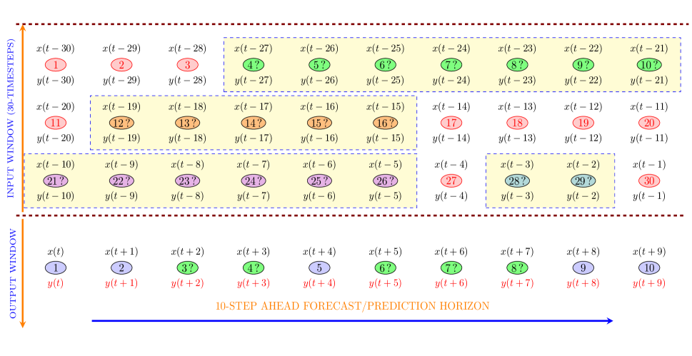
Figure 1. Illustration of an Example Input-Output Window at time $t-1$ of the sequence data.

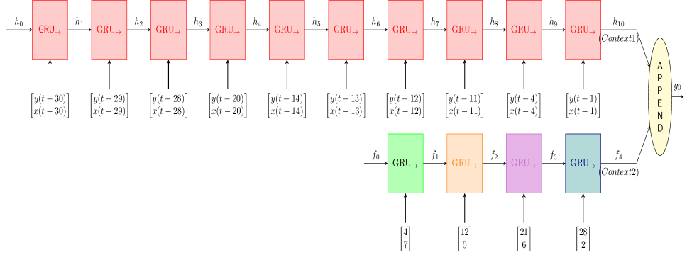
Figure 2. Illustration of the Encoder side of the RNN architecture with reference to Example Sequence of Fig. 1

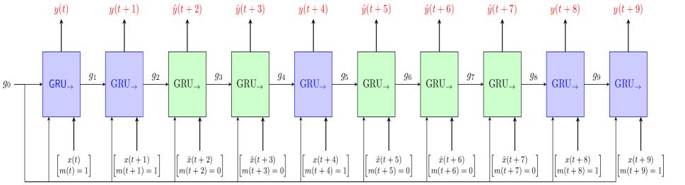
Figure 3. Illustration of the Decoder side (Impute with binary encoding) with reference to Example Sequence of Fig. 1

In this section, we propose a novel encoder decoder architecture which can tackle missing data scenarios without imputation (to the extent possible). Most methods for time-series prediction under missing data either (a) impute the data first and then predict (using standard techniques) OR (b) jointly (or simultaneously) learn the best imputation function and final predictive model. In contrast, we propose a general approach which doesn’t try to learn the imputation function as in the above two approaches. It rather tries to learn the final predictive model without imputation with the missing data entries as they are. In other words, it bases its predictions on the available data and the missingness pattern in the input.

Please note while our approach is very general, it can be particularly attractive in certain situations. In some time series scenarios, nature of data missingness could be such that when data is missing, it mostly happens in a medium/large window of consecutive time points. For instance in health care applications, it is natural for certain patient health parameters not to be monitored for certain long durations of time depending on the diagnosis. In such scenarios imputing the data can be pretty inaccurate especially at time points well into the window. Further if the underlying time series has a high total variation, these imputation errors can be more pronounced. Our approach can be particularly useful in such situations.

3.1.1. Proposed Encoding

We consider sequences or time series where the time of occurrence is an integer (or natural number). In particular, we denote a time series of length $N$ as follows.

(6) $$<\left(x(1),y(1)\right),(x(2),y(2)),\dots(x(t),y(t))\dots(x(N),y(N))>$$

where $t\in\mathbb{N}$, $y(t)$ is the endogenous variable (could be vector-valued) which needs to be forecasted and $x(t)$ (could be vector-valued) is the exogenous variable whose values need to be input into the forecast horizon to forecast the endogenous variable $y(t)$. The assumption of time-series with integer/natural number ticks is necessary for our proposed method. Another key assumption around the type of missingness is to assume that a $(x(t),y(t))$ pair is either completely missing or completely present (all the components).

Key Idea:The intuition of our RNN scheme is to encode the missingness pattern in the input window of a training example as it is, without imputation. This is achieved in a compressed and lossless fashion by using two encoders intelligently. The idea is that this compact input representation can aid the RNN learn better and faster. Fig. 1 and 2 illustrate our overall encoding idea with a general example. The idea is to employ two encoders, one for the available data and the other for the missing data points. The available data points in the input time window are fed in the order of their occurrence into the first encoder in spite of the points not being consecutive. Fig. 1, gives an example input-output window at time tick $t$. The input window dimension is $30$ while the output window is of dimension $10$. The exogenous and endogenous variable/value associated with each time tick of the input window are indicated above and below the (appropriately colored) ellipses. The number in the interior of each of the ellipses indicate the position of the time-tick relative to the start of the window (input or output). Time-ticks where data is missing is additionally quantified with a ${}^{\prime}?^{\prime}$.

Note there are $10$ available data points in the input window each marked in red. Observe that all these $10$ points are fed sequentially to the first encoder as illustrated in Fig. 2. The second encoder identifies the blocks of missing data in the input window. Each block can be uniquely identified by two fields: (a)Start time of the block with reference to the start of the input window (b)width of the block. In Fig. 2, there are $4$ such missing data blocks. Each block of consecutive points is marked by a unique color (also grouped separately and shaded in yellow). In particular, the first block’s relative start position is $4$, while its width is $7$. These two bits of information which identify block $1$ are fed as inputs to the first time-step of the encoder $2$. In general, the $(Starttime,windowwidth)$ information of the $i^{th}$ missing data block in the input-window of the data is fed at the $i^{th}$ time-step of the encoder $2$. As illustrated in Fig. 2, the (start, width) of the $4$ missing data blocks in input window of Fig. 1 are sequentially fed as inputs at $4$ time-steps of encoder $2$. Note the color coding of the $4$ missing data blocks being consistent with the respective GRU block colors to clearly demonstrate our proposed architecture.

This rearranged way of feeding input-window information (without imputation) using two encoders is lossless. Further if data unavailability happens in blocks of large width, our scheme achieves significant compression.

Computational issues: Note that based on our encoding idea, the input part of a training example gets transformed into two vectors (fed to the two encoders) of variable dimension. We exploit this variable length information while training so that the two encoders are sequentially unfolded only to the extent needed. In the presence of data missing in blocks, our encoding scheme can potentially work with larger input windows in comparison to what an impute and predict strategy could due to the vanishing gradient issue. This is because the number of unfolded steps in the two encoders via our scheme can be significantly lower than the input-window size. The example in Fig. 1 is a case in point where a standard encoder would have up-to $30$ time steps, while our intelligent encoding leads to at most $10$ steps per encoder. From a training run-time perspective, for the same input window size, the gradient computation can be faster (compared to an impute and predict strategy) via our two-encoder approach given the reduced number of steps in the unfolded structure.

3.1.2. Decoder Variants

Our above idea of intelligently encoding the available and missing data into two separate layers cannot be employed on the decoder. This is because the decoder is performing a (possibly variable length) multi-step forecasting, where at each time-step the decoder output is used to make a prediction. Basically one needs to retain the identity of each step in the forecast horizon in the unfolded decoder.

Simple Imputation:Perhaps the simplest way to handle missing entries in the output window is to impute the missing entries first using a computationally cheap technique. This could be achieved by a simple mean/median imputation for instance. Now the decoder could be unfolded with inputs and targets at each time-step. Fig. 3 (with $m(t)$ input ignored) illustrates this for example sequence in Fig. 1. Note the imputed values $x$ and $y$ are denoted as $\hat{x}$ and $\hat{y}$ respectively.

Figure 4. Variable Length Unfolding in Decoder (based on Fig. 1

Variable length unfolding: A natural way to tackle missing values in output window is to unfold the decoder based on the first set of consecutively available points from the output window (essentially up to the first missing point). For instance, for example in Fig. 1, we unfold the decoder up to two time-steps only (Fig. 4).

Binary Encoding: The previous approach while plausible would ignore a training example completely if the target at the first time-step of the output window is missing. But this can lead to severe loss of examples. A more intelligent approach would be to additionally introduce a binary vector indicating the presence or absence of data at a time-tick as in (Lipton et al., 2016). This means for every input-output window, we obtain an example (we don’t miss any example) with decoder unfolded for all steps in the output window on each example. The missing values could be imputed based on simple imputation as described above. Fig. 3 indicates the decoder structure with the additional binary input vector ($m(t)$) and imputed missing values for the example in Fig. 1.

GRU-D based Decoder: As explained earlier in related work, GRU-D (Che et al., 2018) in addition to using the masking binary vector also adopts a novel joint impute-learn strategy.

We define formally the binary masking variable, $m_{t}$, as

(7) $$m_{t}=\begin{cases}1,&\text{if }x_{t}\text{ is observed}\\ 0,&\text{otherwise}\end{cases}$$

GRU-D also maintains a time-interval $\delta_{t}$, denoting the distance from its last observation. Formally, for integer time-ticks,

(8) $$\delta_{t}=\begin{cases}1+\delta_{t-1},&\text{if }t>1,m_{t-1}=0\\ 1,&t>1,m_{t-1}=1\\ 0,&t=1.\end{cases}$$

GRU-D which essentially models a decay mechanism based on the last observation’s distance. The decay factor is modelled for each input variable using a monotonically decreasing function of $\delta_{t}^{L}$ ranging between $0$ and $1$.

(9) $$\gamma_{t}=exp\{-max(0,W_{\gamma}\delta_{t}+b_{\gamma})\}$$

The modified input that is input to the GRU unit is now

(10) $$\hat{x}(t)=m_{t}x(t)+(1-m_{t})(\gamma_{t}x^{L}(t)+(1-\gamma_{t})\tilde{x})$$

where $x^{L}(t)$ is the last observation to the left of $t$ and $\tilde{x}$ is the empirical mean of $x(t)$. Replacing $u(t)$ by $\hat{x}(t)$ in eqns. (2)-(5) is what a GRU-D recurrent unit is by incorporating input decay alone. Enhancing the architecture of Fig. 3 using modified exogenous inputs based on eqns. (7)-(10) gives us a GRU-D based decoder.

3.2. Training on multi-sequence data

Building sequence-specific models for multi-sequence data, when per-sequence data is less, may be a poor strategy. It can be further compounded if the exogenous variable additionally shows very little variation per sequence. We propose a heuristic strategy to adapt our above architecture (primarily for single sequences) to such scenarios. The idea is to build one common background model which can tackle the per-sequence data sparsity. We perform a sequence-specific scaling of each of the input-output windows (for both the endogenous and exogenous variables) depending on the sequence from which a particular input-output window was constructed. These normalized examples are used to train a common background model. During prediction the model output is re-scaled in a sequence-specific fashion.

4. Results

We first describe the data sets used for testing, followed by error metrics and hyper-parameters for evaluation, baselines and performance results in comparison to them.

4.1. Data Sets

Our first data set D1 validates our proposed approach at a single sequence level with about $4$ sequences. Synthetic masking is employed here. The next two data sets are used to vindicate our approach on multi-sequence data. In particular, synthetic masking is employed in D3, while D2 has missing data points naturally. We provide more details of these data-sets next.

• D1: M5 data-set is a publicly available data-set from Walmart and contains the unit sales of different products on a daily basis spanning 5.4 years. This data is distributed across 12 different aggregation levels. We pick sequences from level $12$ where sales and prices are available at a product and store level (lowest level with no sales aggregation). Price is used as exogenous input here. While this level contains little more than $30\,000$ sequences, we pick $4$ sequences from here with high total variation (referred to as D1). We essentially pick the hardest sequences which exhibit sufficient variation. The total variation of a $T$ length sequence $x$ is defined as

  (11) $$TV=\sum_{i=2}^{T}|(x(i+1)-x(i)|$$

  We test our architecture separately on each of these $4$ sequences by synthetically masking with large width windows.

• D2: This is weekly sales data at an item level from a brick and mortar retail chain (confidential) of a category of items collected over $2$ years. There is data missing here naturally on account of no sales and other factors. Per-sequence data is less while price which is the exogenous variable has little variation per sequence. Sequences from this category whose fraction of missing points were anywhere less than $60\%$ were chosen to form $D2$. It consists of $1288$ sequences.

• D3: This is publicly available from Walmart. The measurements are weekly sales at a department level of multiple departments across 45 Walmart stores. The price information was chosen as exogenous variable. The data is collected across $3$ years and it’s a multiple time-series data. The whole data set consists of $2628$ sequences. For the purpose of this paper, we ranked sequences based on the total variation of the sales and considered the top $20\%$ of the sequences (denoted as D3) for testing.

Given D2, D3 are multi-sequence data sets with limited per-sequence data, we employ the heuristic background model building idea described in Sec. 3.2. over a given single-sequence method.

4.2. Error metrics and Hyper-parameter choices

We consider the following two error metrics.

• MAPE (Mean Absolute Percentage Error)

• MASE (Mean Absolute Scale Error(Hyndman and Koehler, 2006))

The APE is relative error (RE) expressed in percentage. If $\widehat{X}$ is predicted value, while $X$ is the true value, RE = $(\widehat{X}-X)/X$. In the multi-step setting, APE is computed for each step and is averaged over all steps to obtain the MAPE for one window of the prediction horizon. APE while has the advantage of being a scale independent metric, can assume abnormally high values and can be misleading when the true value is very low. An alternative complementary error metric which is scale-free could be MASE.

The MASE is computed with reference to a baseline metric. The choice of baseline is typically the copy previous predictor, which just replicates the previous observed value as the prediction for the next step. For a given window of one prediction horizon of $K$ steps ahead, let us denote the $i^{th}$ step error by $|\widehat{X}_{i}-X_{i}|$. The $i^{th}$ scaled error is defined as

(12) $$e_{s}^{i}=\frac{|\widehat{X}_{i}-X_{i}|}{\frac{1}{n-K}\sum_{j=K+1}^{n}|X_{j}-X_{j-K}|}$$

where $n$ is no. of data points in the training set. The normalizing factor is the average $i^{th}$ step-ahead error of the copy-previous baseline on the training set. Hence the MASE on a multi-step prediction window $w$ of size $K$ will be

(13) $$MASE(w,K)=\frac{1}{K}\sum_{j=1}^{K}e_{s}^{j}$$

Table 1 describes the broad choice of hyper-parameters during training in our experiments.

Table 1. Model parameters during training.

Parameters	Description
Batch size	64/256
Number of Hidden layers	1/2
Hidden vector dimensionality	7/9
Optimizer	RMSProp / Adam

4.3. Baselines and Proposed Approaches

We benchmark two of the discussed decoder variants (Sec.3.1.2): (a)Simple (Mean) Imputation denoted as DEMI (b)GRU-D based decoder imputation denoted as DEGD. DE refers to double encoder or the two RNN layers used to encode input window (Fig. 2). Recall from Sec. 3.1.2 that ‘variable length unfolding’ variant can suffer from severe loss of examples while the ‘Binary encoding’ variant is a special case of GRU-D based variant. Hence, we benchmark DEMI and DEGD only. The baselines we benchmark our method against are as follows:

1. BEDXM - post mean imputation (in all missing points) run a Basic Encoder-Decoder (with one encoder capturing immediate lags) with exogenous inputs as in (Wen et al., 2017).

2. BEDXL - Consider any band of missing points. The center of the band is imputed with the mean while from both the left and right end the missing points are now linearly interpolated. Next use (Wen et al., 2017) as above. It uses a simple imputation method but utilizes both the right and left end information of any gap unlike (Che et al., 2018).

3. GRU-D(Che et al., 2018) - at both the encoder and decoder, we use the GRU-D unit to achieve multi-step forecasting (something unexplored in the original (Che et al., 2018) paper).

4. WIAED(Cinar et al., 2018) - which learns the position-based weighted influence of imputed values followed by attention layer on the encoder-decoder framework.

4.3.1. Assessing significance of mean error differences statistically

We have conducted a Welch t-test (unequal variance) based significance assessment (across all relevant experiments) under both the mean metric (MASE, MAPE) differences (Proposed vs Baseline) with a significance level of 0.05 for null hypothesis rejection. The best performing method’s error is highlighted in bold if its MASE/MAPE improvement over every other method is statistically significant. We allow for highlighting the second/third best errors in situations when the mean error differences between the best and second best errors are statistically insignificant.

4.3.2. Synthetic Masking

The masking process adopted is as follows. We scan the time-series sequentially from the start. At each step, we essentially decide if a masking has to be carried out starting from the current step. Towards this, we toss a coin with a variable heads probability $q$. If tails, we decide against masking from the current step and move on. On heads, we decide to mask from current step. After seeing a head every time, a decision of how many consecutive data points to mask needs to be taken. Towards this, we consider $\mathcal{T}_{w}$, which is set of window lengths from which we uniformly sample a specific length. Let $T_{w}$ denote the window length sampled from $\mathcal{T}_{w}$. For the next masking window starting position, we choose $q=1/T_{w}$. This strategy assures that about $50\%$ of the data points are missing because for every ${T}_{w}$ points removed, we retain the next ${T}_{w}$ points (in expectation). Initial $q$ is set to $0.05$.

Synthetic masking has the following advantage. Since the underlying true data before masking is available, one can assess the efficacy of training on a separate test set for every step of the prediction horizon.

4.4. Results on D1 (after synthetic masking)

For D1, the forecast horizon was set to be $28$ days (K = 28). The choice of $K=28$ would mean about $4$ weeks ahead (which is a meaningful and not an overly long forecast horizon). This was also the forecast horizon of the $M5$ challenge. A test size of $127$ days (time-points) out of $1941$ time points was set aside for each sequence in D1. This means we tested for $100$ output windows of width $28$ per sequence.

To illustrate on D1 (data is not missing), we artificially simulate masking using long masking windows. Tab. 2 provides errors of all relevant methods. Results indicate superior performance of both DEMI and DEGD with best case MAPE improvements per baseline of $14\%$, $8\%$, $4\%$ and $28\%$ with respect to BEDXM, BEDXL, GRU-D and WIAED respectively. Similarly, the best case MASE improvements per baseline were $0.17$, $0.16$, $0.05$ and $0.39$ respectively. Also note all improvements of the proposed approaches are statistically significant.

Table 2. D1 results: $\mathcal{T}_{w}=\{30,31,32,\dots,39,40\}$, Input-Window width=$200$.

Seq ID	DEMI	DEGD	BEDXM	BEDXL	GRU-D	WIAED
$FOODS\_3\_714$	(0.47,38)	(0.46,38)	(0.56,46)	(0.56,46)	(0.49,41)	(0.48,39)
$FOODS\_3\_252$	(0.51,23)	(0.51,23)	(0.54,26)	(0.57,25)	(0.55,25)	(0.74,33)
$FOODS\_3\_080$	(0.16,7)	(0.15,7)	(0.32,21)	(0.31,15)	(0.20,11)	(0.54,35)
$FOOD\_3\_090$	(0.29,19)	(0.29,19)	(0.41,26)	(0.45,27)	(0.32,21)	(0.50,41)

4.5. Results on D2

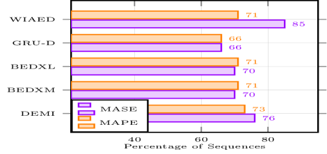
Figure 5. Percentage of sequences (out of $940$ on which at least one method’s MASE $<1$) where DEGD does better.

Table 3. Max, Avg and Min of MASE across all relevant $940$ sequences (on which at least one method’s MASE $<1$)

	MASE based
Method	Max	Avg	Min
DEMI	21.44	1.79	0.004
DEGD	19.61	0.43	0.001
BEDXM	17.26	1.34	0.001
BEDXL	16.98	1.37	0.002
GRU-D	16.87	0.52	0.0002
WIAED	24.11	0.93	0.005

For D2, input window size is chosen to be $20$, while the prediction horizon chosen was of length $K=12$ (decoder length OR output window size), which is a $3$-month ahead forecast horizon. This choice of input and output window length (per example) results in a reasonably long forecast horizon while also generating sufficient number of input-output examples per sequence given that we have about $104$ weeks of data points per sequence. We tested for $6$ output windows of width $12$ on a $17$ week (separately kept) test set per sequence.

For about $348$ items, MASE $>1$, for all baselines and the proposed methods. which meant these items could be tackled better by the simple copy previous baseline. We hence kept these items aside and concentrate on the remaining $940$, on each of which at least one of the baselines OR proposed approaches have MASE $<1$. Fig. 5 gives a detailed breakup of the percentage of these $940$ sequences on which DEGD did better compared to the $3$ baselines. It demonstrates that DEGD does better on at least $66\%$ of sequences and up to $85\%$, compared to all baselines.

Tab. 3 gives the average, max and min across sequences (of MASE) for all methods. It demonstrates that on an average DEGD does better than all baselines. MASE improvements are up to $0.94$. Tab. 4 looks at the (conditional) average MASE under two conditions with respect to each baseline: (i)average over those sequences on which DEGD fares better, (ii)average over those sequences on which the baseline does better. At this level, we observe MASE improvements of at least $0.22$ while up to $1.58$.

Table 4. Average MASE on $940$ relevant sequences when (i)DEGD fares better (ii)Baseline fares better.

	DEGD better			Baseline better
Method	DEGD	BLine	Diff	DEGD	BLine	Diff
DEMI	0.26	2.18	1.92	0.97	0.59	0.38
BEDXM	0.21	1.75	1.54	0.94	0.40	0.54
BEDL	0.21	1.79	1.58	0.93	0.41	0.52
GRU-D	0.24	0.46	0.22	0.80	0.64	0.16
WIAED	0.34	0.98	0.64	0.95	0.69	0.26

4.6. Results on D3 after synthetic masking

As explained earlier, we perform a synthetic masking first. Note the per-sequence length here is about $150$ points. Compared to D1, the input window length has to chosen to be comparatively lower (chosen to be $20$ here as in D2) to obtain reasonable number of input-output examples from each sequence. This means the masking window length has to be proportionately less (compared to that of D1).

A test size of 15 weeks (time-points) was set aside for each sequence (out of about $150$ weeks) in D3. We choose K = 10 time-steps in the decoder (output window length) for training which means forecast time-horizon would be about $2.5$ months, a reasonably long forecast window which also allows for sufficiently many input output examples from each sequence. We tested for $6$ output windows (as in D2) of width $10$ on the $15$ week test set per sequence.

Fig. 6 gives a detailed breakup of percentage of sequences on which DEMI did better compared to the $4$ baselines. It demonstrates that DEMI does better on at least $52\%$ of the sequences and up to $59\%$ compared to all considered baselines. A similar plot is obtained when DEGD is compared with the $4$ baselines as shown in Fig. 7. This clearly indicates similar performance of DEGD and DEMI on D3.

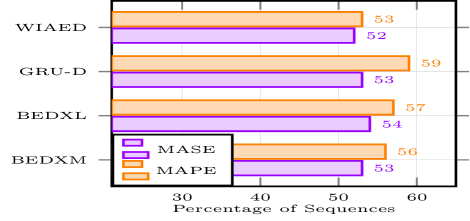
Figure 6. Percentage of sequences where DEMI does better. $q=0.05$, $\mathcal{T}_{w}=\{6,7,8,9,10\}$.

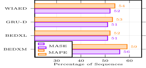
Figure 7. Percentage of sequences where DEGD does better. $q=0.05$, $\mathcal{T}_{w}=\{6,7,8,9,10\}$.

Tab. 5 gives the average, max and min across sequences (of MASE and MAPE) for all methods. It demonstrates that on an average DEMI does better than all baselines based on both these complementary metrics. MASE improvements are up to $0.10$ while the MAPE improvements are up to $5\%$. Tab. 6 looks at the (conditional) average MASE under two conditions with respect to each baseline: (i)average over those sequences on which DEMI fares better, (ii)average over those sequences on which the baseline does better. At this level, MASE improvements of at least $0.28$ while up to $0.60$ are observed. Tab. 7 considers a similar (conditional) average MAPE. At this level of MAPE, there are improvements of at least $11\%$ to up to $18\%$. Overall our results on D3 indicate that our approach is viable even when the masking window length is low.

Table 5. Max, Avg, Min of MASE/MAPE across all sequences

	MASE based			MAPE based in $\%$
	Max	Avg	Min	Max	Avg	Min
DEMI	4.03	0.93	0.29	349	31	2
DEGD	3.77	0.94	0.08	397	32	0.4
BEDXM	3.62	0.99	0.08	347	36	0.9
BEDXL	3.43	0.96	0.03	382	35	0.4
GRU-D	3.53	0.96	0.08	318	33	2
WIAED	4.58	1.03	0.09	250	33	0.7

Table 6. Average MASE on sequences where (i)DEMI fares better (ii)Baseline fares better.

	DEMI better			Baseline better
Method	DEMI	BLine	Diff	DEMI	BLine	Diff
DEGD	0.84	1.12	0.28	1.04	0.75	0.29
BEDXM	0.84	1.24	0.40	1.03	0.71	0.32
BEDXL	0.84	1.18	0.34	1.04	0.71	0.33
GRU-D	0.84	1.14	0.30	1.03	0.76	0.27
WIAED	0.86	1.46	0.60	1.00	0.58	0.42

Table 7. Average MAPE on sequences where (i)DEMI fares better (ii)Baseline fares better.

	DEMI better			Baseline better
Method	DEMI	BLine	Diff	DEMI	BLine	Diff
DEGD	28	39	11	36	23	13
BEDXM	29	47	18	34	21	13
BEDXL	32	47	15	30	19	11
GRU-D	28	40	12	37	24	13
WIAED	28	44	16	35	17	18

5. Conclusions and Future Work

We proposed a novel lossless, compressed encoding scheme of the input window sequence using RNNs. This is equally applicable for classification and forecasting. Based on this novel scheme, we proposed an encoder-decoder framework for a general multi-step forecasting with possible exogenous inputs. We showed that multiple interesting variations are possible on the associated decoder. We demonstrated the utility of this ED framework on multiple data-sets where our proposed approach was outperforming the current state-of-art RNN baselines. In particular, our approaches demonstrated superior or comparable performances in both scenarios where (i)data was synthetically masked with varied masking window length choices (data-sets D1 and D3) and (ii)when data was naturally missing (as in D2). Further, our experiments also indicate that our DEGD variant was the more robust variant in performance (compared to DEMI which performed poorly on D2). We also demonstrated the applicability of our proposed architectures on both single (D1) and multi sequence data sets (D2 and D3). As future work, we would like to validate our approach on classification tasks. We would also like to explore approaches where target imputation can be avoided (before model building) in forecasting applications.

References

- (1)
- Bengio and Gingras (1995) Yoshua Bengio and Francois Gingras. 1995. Recurrent Neural Networks for Missing or Asynchronous Data. In Proceedings of the 8th International Conference on Neural Information Processing Systems. MIT Press, Cambridge, MA, USA, 395–401.
- Che et al. (2018) Zhengping Che, Sanjay Purushotham, Kyunghyun Cho, David Sontag, and Yan Liu. 2018. Recurrent Neural Networks for Multivariate Time Series with Missing Values. Scientific Reports 8 (Jun 2018).
- Cho et al. (2014) Kyunghyun Cho, Bart van Merriënboer, Caglar Gulcehre, Dzmitry Bahdanau, Fethi Bougares, Holger Schwenk, and Yoshua Bengio. 2014. Learning Phrase Representations using RNN Encoder–Decoder for Statistical Machine Translation. In Proceedings of the 2014 Conference on Empirical Methods in Natural Language Processing (EMNLP). 1724–1734.
- Chung et al. (2014) Junyoung Chung, Caglar Gulcehre, KyungHyun Cho, and Yoshua Bengio. 2014. Empirical Evaluation of Gated Recurrent Neural Networks on Sequence Modeling. In NIPS 2014 Deep Learning and Representation Learning Workshop.
- Cinar et al. (2018) Yagmur Gizem Cinar, Hamid Mirisaee, Parantapa Goswami, Eric Gaussier, and Ali Aït-Bachir. 2018. Period-aware content attention RNNs for time series forecasting with missing values. Neurocomputing 312 (2018), 177–186.
- Elman (1990) Jeffrey L. Elman. 1990. Finding structure in time. Cognitive Science 14, 2 (1990), 179–211.
- García-Laencina et al. (2010) Pedro J. García-Laencina, José-Luis Sancho-Gómez, and Aníbal R. Figueiras-Vidal. 2010. Pattern Classification with Missing Data: A Review. Neural Comput. Appl. 19, 2 (March 2010), 263–282.
- Graves and Jaitly (2014) Alex Graves and Navdeep Jaitly. 2014. Towards End-to-End Speech Recognition with Recurrent Neural Networks. In Proceedings of the 31st International Conference on International Conference on Machine Learning - Volume 32. 1764–1772.
- Graves et al. (2009) Alex Graves, Marcus Liwicki, Santiago Fernández, Roman Bertolami, Horst Bunke, and Jürgen Schmidhuber. 2009. A Novel Connectionist System for Unconstrained Handwriting Recognition. IEEE Trans. Pattern Anal. Mach. Intell. 31, 5 (May 2009), 855–868.
- Graves et al. (2013) A. Graves, A. Mohamed, and G. Hinton. 2013. Speech recognition with deep recurrent neural networks. In 2013 IEEE International Conference on Acoustics, Speech and Signal Processing. 6645–6649.
- Gruber and Jockisch (2020) Nicole Gruber and Alfred Jockisch. 2020. Are GRU cells more specific and LSTM cells more sensitive in motive classification of text? Front. Artif. Intell. (2020).
- Gupta et al. (2017) Ankita Gupta, Gurunath Gurrala, and Pidaparthy S. Sastry. 2017. Instability Prediction in Power Systems Using Recurrent Neural Networks. In Proceedings of the 26th International Joint Conference on Artificial Intelligence. AAAI Press, 1795–1801.
- Hochreiter and Schmidhuber (1997) Sepp Hochreiter and Jürgen Schmidhuber. 1997. Long Short-Term Memory. Neural Comput. 9, 8 (Nov. 1997), 1735–1780.
- Hyndman and Koehler (2006) Rob J. Hyndman and Anne B. Koehler. 2006. Another look at measures of forecast accuracy. International Journal of Forecasting 22, 4 (2006), 679–688.
- Johnson (2013) Sharon A. Johnson. 2013. Splines. Springer US, Boston, MA, 1443–46.
- Jordan (1988) Michael I. Jordan. 1988. Supervised Learning and Systems with Excess Degrees of Freedom. Technical Report. USA.
- Kiros et al. (2014) Ryan Kiros, Ruslan Salakhutdinov, and Richard S. Zemel. 2014. Unifying Visual-Semantic Embeddings with Multimodal Neural Language Models. CoRR abs/1411.2539 (2014).
- Koren et al. (2009) Yehuda Koren, Robert Bell, and Chris Volinsky. 2009. Matrix Factorization Techniques for Recommender Systems. Computer 42, 8 (Aug. 2009), 30–37.
- Lim and Zohren (2021) Bryan Lim and Stefan Zohren. 2021. Time-series forecasting with deep learning: a survey. Phil. Trans. R. Soc. A. 379, 2194 (2021), 40–48.
- Lipton et al. (2016) Zachary C Lipton, David Kale, and Randall Wetzel. 2016. Directly Modeling Missing Data in Sequences with RNNs: Improved Classification of Clinical Time Series. In Proceedings of the 1st Machine Learning for Healthcare Conference, Vol. 56. PMLR, 253–270.
- Lu et al. (2015) Liang Lu, Xingxing Zhang, Kyunghyun Cho, and Steve Renals. 2015. A study of the recurrent neural network encoder-decoder for large vocabulary speech recognition. In Proceedings of the 16th Annual Conference of the International Speech Communication Association, INTERSPEECH. 3249–3253.
- Mondal and Percival (2010) Debashis Mondal and Donald Percival. 2010. Wavelet variance analysis for gappy time series. Annals of the Institute of Statistical Mathematics 62, 5 (October 2010), 943–966.
- Parveen and D. Green (2001) S. Parveen and P. D. Green. 2001. Speech Recognition with Missing Data Using Recurrent Neural Nets. In Proceedings of the 14th International Conference on Neural Information Processing Systems: Natural and Synthetic. MIT Press, Cambridge, MA, USA, 1189–1195.
- Ravanelli et al. (2018) Mirco Ravanelli, Philemon Brakel, Maurizio Omologo, and Yoshua Bengio. 2018. Light Gated Recurrent Units for Speech Recognition. IEEE Transactions on Emerging Topics in Computational Intelligence 2, 2 (Apr 2018), 92–102.
- Rehfeld et al. (2011) Kira Rehfeld, Norbert Marwan, Jobst Heitzig, and Jürgen Kurths. 2011. Comparison of correlation analysis techniques for irregularly sampled time series. Nonlinear Processes in Geophysics 18, 3 (July 2011), 389–404.
- Sutskever et al. (2014) Ilya Sutskever, Oriol Vinyals, and Quoc V. Le. 2014. Sequence to Sequence Learning with Neural Networks. In Proceedings of the 27th International Conference on Neural Information Processing Systems - Volume 2. 3104–3112.
- Tresp and Briegel (1997) Volker Tresp and Thomas Briegel. 1997. A Solution for Missing Data in Recurrent Neural Networks with an Application to Blood Glucose Prediction. In Proceedings of the 10th International Conference on Neural Information Processing Systems. MIT Press, Cambridge, MA, USA, 971–977.
- van den Oord et al. (2016) Aäron van den Oord, Sander Dieleman, Heiga Zen, Karen Simonyan, Oriol Vinyals, Alex Graves, Nal Kalchbrenner, Andrew W. Senior, and Koray Kavukcuoglu. 2016. WaveNet: A Generative Model for Raw Audio. CoRR abs/1609.03499 (2016).
- Wang and Tax (2016) Feng Wang and David M. J. Tax. 2016. Survey on the attention based RNN model and its applications in computer vision. CoRR abs/1601.06823 (2016).
- Wen et al. (2017) Ruofeng Wen, Kari Torkkola, Balakrishnan Narayanaswamy, and Dhruv Madeka. 2017. A Multi-Horizon Quantile Recurrent Forecaster. In The 31st Conference on Neural Information Processing Systems (NIPS 2017), Time Series Workshop.
- Xing et al. (2010) Zhengzheng Xing, Jian Pei, and Eamonn Keogh. 2010. A Brief Survey on Sequence Classification. SIGKDD Explor. Newsl. 12, 1 (Nov. 2010), 40–48.
- Xu et al. (2015) Kelvin Xu, Jimmy Lei Ba, Ryan Kiros, Kyunghyun Cho, Aaron Courville, Ruslan Salakhutdinov, Richard S. Zemel, and Yoshua Bengio. 2015. Show, Attend and Tell: Neural Image Caption Generation with Visual Attention. In Proceedings of the 32nd International Conference on International Conference on Machine Learning - Volume 37. 2048–2057.