Dynamic State Estimation-Based Protection
for Induction Motor Loads

Abstract

Ensuring protective device coordination is critical to maintain the resilience and improve the reliability of large microgrids. Inverter-interfaced generation, however, poses significant challenges when designing protection systems. Traditional time-overcurrent protective devices are unsuitable on account of the lack of fault current. Present industry practice is to force all inverters to shut down during faults, which prevents large microgrids from operating in a resilient and reliable manner. Dynamic state estimation (DSE) has been proposed for line protection, and more recently for the protection of load buses or downstream radial portions of microgrids. However, only passive loads with series resistive-inductive loads have been tested with DSE, even though the behavior of dynamic loads – such as induction motors or power electronics – may differ significantly during faults. This paper considers the case of applying DSE to protecting a load bus serving a three-phase induction motor.

I Introduction

Microgrids have been a key tool to integrate distributed renewable energy resources into the bulk energy system. When operating under islanded conditions, microgrids are reliant upon not only inverter run energy storage, but renewable resources as well. Although they are reasonably reliable, economical, and low greenhouse gas contributors, inverter fed resources – commonly photovoltaic panels and wind farms – suffer from issues such as availability – variability in the levels of irradiation and wind available during the day – that makes their power output variable and limited system inertia [1]. Under faulted conditions, the current drawn by the system when fed by a synchronous machine is significantly higher and is thus ideal for an overcurrent relay to provide protection. However, an inverter is limited at the amount of current it can provide, therefore limiting the ability to use conventional devices to provide protection; also, the response of an inverter fed device to a change is fast, and thus control devices must respond quickly as well [2].

Electrical loads today are dominated by power electronic converter run devices, and single-phase and three-phase induction machines. Most devices have an inverter involved for powering them, while induction motors – the mainstay of HVAC systems, agricultural systems, and several industrial applications owing to the low cost of construction, easy maintenance, and high efficiency – require protection mechanisms in place for safe and reliable operation [3, 4]. Induction motors, owing to their non-linear behavior, undergo prolonged periods of transiency until they reach steady-state; this warrants the need to ensure that system parameters during the period of transition does not reach extremely high values [5]. Under faulted conditions – be it stator faults, rotor faults, or external line faults – the current drawn by the machine is significantly higher, which in turn can impact the health of the device [6]. This becomes more profound in an inverter fed microgrid, where the system has limited to no inertia – due to the lack of stored kinetic energy – that could be harvested to adjust to intermittent loading conditions or fault conditions [7]. Consequently, it becomes important to study the protection of induction motors in a microgrid.

Protection methods enable the resilient and reliable operation of microgrids by maintaining protective device coordination to minimize the extent of outages. Conventional approaches have focused on protecting just the inverters, resulting in the whole microgrid shutting down during a fault; additionally, these approaches do not scale to large networks [8]. Distance relaying techniques have been explored for protecting inverter-interfaced microgrids: Dewadasa et al. [9] suggested limiting the per phase current in faulted conditions by using distance relaying; Kar et al. [10] demonstrated the use of differential relaying based on the discrete S-transform performed on the change in system current magnitude under fault conditions; and Huang [11] used an adaptive protection system, in which multiple relays co-ordinate among themselves to predict the occurrence of a fault and recommend corrective action. All these, however, employ the use of legacy programmed protection devices and does not cater to system dynamics or protect the system against bi-directional power flow. It is unequivocal that new protection methods are needed to support the deployment of large microgrids.

Settingless protection addresses these shortcomings by employing Dynamic State Estimation (DSE) to generate system measurements such that protective control action is determined based on the mismatch between the measurements and estimates generated using accurate system models [12, 13, 14]. DSE allows for increased accuracy in tracking system dynamics and better system estimates, therefore allowing better system operation and control [15]; it can accurately track system dynamics and can effectively predict the fault characteristics across microgrids of varying sizes under high penetration of renewable energy resources [16]. DSE has been used to develop centralized protection schemes [16, 17] and to detect hidden failures in substation protection systems [18]. More recently, it has been proposed for protection of load buses [19] and downstream radial sections of microgrids [13, 20]. It is also finding an increased relevance in power system operation and monitoring applications [21], owing to the implementation of accurate dynamic models that provide reliable estimates, improved oscillation monitoring, and increased potential for decentralized control [15].

This work investigates the application of DSE for load bus protection, while considering the dynamic behavior of an induction motor. Section II presents the dynamic simulation model selected for an induction motor, the DSE formulation derived from the simulation model, and the solution method for the DSE problem. Section III presents a case study system based on a numerical simulation of an induction motor under several different fault scenarios. Section IV presents experimental results from the numerical simulation and DSE algorithm. Finally, Section V summarizes the conclusions regarding the utility of DSE for load bus protection.

II Methodology

The induction machine model used in this work is a Julia [22] implementation of the MATLAB asynchronous machine model [23], which has been developed using the induction motor models proposed by [3] and [24].

II-A 5^th- order Induction Motor State Estimation Model

To convert time-varying induction motor inductances into constant values, in order to simplify the solution of the governing differential equations, the quantities for the machine inputs and states were converted into a rotating reference frame, as described below.

Rotating reference-frame transform from [3] (3.3-4):

$$\begin{split}&\begin{bmatrix}v_{q}(t)\\ v_{d}(t)\\ v_{0}(t)\end{bmatrix}=\\ &=\frac{2}{3}\begin{bmatrix}\cos(\theta(t))&\cos(\theta(t)-\alpha)&\cos(\theta(t)+\alpha)\\ \sin(\theta(t))&\sin(\theta(t)-\alpha)&\sin(\theta(t)+\alpha)\\ 1/2&1/2&1/2\end{bmatrix}\begin{bmatrix}v_{a}(t)\\ v_{b}(t)\\ v_{c}(t)\end{bmatrix}\end{split}$$ (1)

where $\alpha=\frac{2}{3}\pi$; $v_{a}(t)$, $v_{b}(t)$, and $v_{c}(t)$ are the line-ground voltages on phases A, B and C, respectively; and $v_{q}(t)$, $v_{d}(t)$, and $v_{0}(t)$ are the voltages on the q, d, and 0 axes, respectively.

Magnetizing flux linkages from [3] (6.14-15) – (6.14-17):

$$\dot{\psi}_{qs}(t)=v_{qs}(t)-\omega\cdot\psi_{ds}(t)-R_{s}\cdot i_{qs}(t)$$ (2)

where $v_{qs}(t)$ is the stator voltage in the q-axis; and $\psi_{ds}(t)$ is the stator flux in the d-axis.

$$\dot{\psi}_{ds}(t)=v_{ds}(t)+\omega\cdot\psi_{qs}(t)-R_{s}\cdot i_{ds}(t)$$ (3)

where $v_{ds}(t)$ is the stator voltage in the d-axis; and $\psi_{qs}(t)$ is the stator flux in the q-axis.

$$\dot{\psi}_{qr}^{\prime}(t)=v_{qr}^{\prime}(t)-(\omega-\omega_{r})\cdot\psi_{dr}^{\prime}(t)-R_{r}^{\prime}\cdot i_{qr}^{\prime}(t)$$ (4)

where $v_{qr}^{\prime}(t)$ is the rotor voltage referred to the stator in the q-axis; and $\psi_{dr}^{\prime}(t)$ is the rotor flux in the d-axis referred to the stator.

$$\dot{\psi}_{dr}^{\prime}(t)=v_{dr}^{\prime}(t)+(\omega-\omega_{r})\cdot\psi_{qr}^{\prime}(t)-R_{r}^{\prime}\cdot i_{dr}^{\prime}(t)$$ (5)

where $v_{dr}^{\prime}(t)$ is the rotor voltage referred to the stator in the d-axis; and $\psi_{qr}^{\prime}(t)$ is the rotor flux in the q-axis referred to the stator.

In Equations (2) – (5): $\omega(t)$ is the synchronous speed; $R_{s}$ is the stator resistance; $R^{\prime}_{r}$ is the rotor resistance; and $\omega_{r}(t)=P\omega(t)$, where $P$ is the number of poles in the induction machine and $\omega_{r}(t)$ is the angular velocity of the rotor.

Flux linkages expressed as a function of currents, from [3] (6.14-4) – (6.14-6):

$${\psi}_{qs}(t)=L_{s}\cdot i_{qs}(t)+L_{m}\cdot i_{qr}^{\prime}(t)$$ (6)

$${\psi}_{ds}(t)=L_{s}\cdot i_{ds}(t)+L_{m}\cdot i_{dr}^{\prime}(t)$$ (7)

$${\psi}_{qs}(t)=L_{r}^{\prime}\cdot i_{qr}^{\prime}(t)+L_{m}\cdot i_{qs}(t)$$ (8)

$${\psi}_{qs}(t)=L_{r}^{\prime}\cdot i_{qr}^{\prime}(t)+L_{m}\cdot i_{qs}(t)$$ (9)

In Equations (2) – (9): $i_{qs}(t)$ and $i_{ds}(t)$ are the stator currents; $i_{qr}(t)^{\prime}$ and $i_{dr}(t)^{\prime}$ are the rotor currents referred to the stator; $L_{s}$ is the stator inductance; $L_{r}^{\prime}$ is the rotor inductance; and $L_{m}$ is the magnetizing inductance.

Electrical torque from [3] (6.6-16)–(6.6-17):

$$T_{e}(t) =\frac{3}{2}\cdot\frac{P}{2}\cdot\frac{1}{\omega}\cdot\left(\psi^{\prime}_{qr}(t)\cdot i^{\prime}_{dr}(t)-\psi^{\prime}_{dr}(t)\cdot i^{\prime}_{qr}(t)\right)$$ (10)

$$=\frac{3}{2}\cdot\frac{P}{2}\cdot\frac{L_{m}}{D}\frac{1}{\omega}\cdot\left(\psi_{qs}(t)\cdot\psi^{\prime}_{dr}(t)-\psi^{\prime}_{qr}(t)\cdot\psi_{ds}(t)\right)$$ (11)

Rotor speed from [3] (6.3-8):

$$\dot{\omega}_{m}(t)=\frac{P}{2J}\cdot\left(T_{e}(t)-F\cdot w_{m}-T_{m}(t)\right)$$ (12)

where $T_{e}$ is the electromagnetic torque; $T_{m}$ is the shaft mechanical torque; $J$ is the combined rotor and load inertia coefficient; and $F$ is the combined rotor and load viscous friction coefficient.

II-B 5^th- order Induction Motor State Estimation Model

To perform state estimation, the above equations from the simulation model were reformulated as State-Output Mapping, described in [25].

Observables

$$\mathbf{y}=\begin{bmatrix}v_{q}(t)&v_{d}(t)&i_{q}(t)&i_{d}(t)&\\ z_{\psi_{qs}}(t)&z_{\psi_{ds}}(t)&z_{\psi^{\prime}_{qr}}(t)&z_{\psi^{\prime}_{dr}}(t)&z_{Te}(t)\end{bmatrix}^{T}$$ (13)

State

$$\mathbf{x}=\begin{bmatrix}\psi_{qs}(t)&\psi_{ds}&\psi^{\prime}_{qr}(t)&\psi^{\prime}_{dr}(t)&T_{e}(t)&\omega_{r}(t)\end{bmatrix}^{T}$$ (14)

State-Output Mapping

The algebraic voltage equations:

$$\begin{split}v_{qs}(t)=\frac{R_{s}\cdot L^{\prime}_{lr}}{D}\cdot\psi_{ds}(t)-\omega(t)\cdot\psi_{qs}(t)-\frac{R_{s}\cdot L_{m}}{D}\cdot\psi^{\prime}_{dr}(t)\end{split}$$ (15)

$$\begin{split}v_{ds}(t)=\frac{R_{s}\cdot L^{\prime}_{lr}}{D}\cdot\psi_{qs}(t)+\omega(t)\cdot\psi_{ds}(t)-\frac{R_{s}\cdot L_{m}}{D}\cdot\psi^{\prime}_{qr}(t)\end{split}$$ (16)

Algebraic current equations:

$$\begin{split}i_{qs}(t)=\frac{L^{\prime}_{lr}}{D}\cdot\psi_{ds}(t)-\frac{L_{m}}{D}\cdot\psi^{\prime}_{dr}(t)\end{split}$$ (17)

$$\begin{split}i_{qs}(t)=\frac{L^{\prime}_{lr}}{D}\cdot\psi_{qs}(t)-\frac{L_{m}}{D}\cdot\psi^{\prime}_{qr}(t)\end{split}$$ (18)

$$\begin{split}i^{\prime}_{qr}(t)=\frac{1}{L_{m}}\cdot\left(\psi_{qs}(t)-L_{s}\cdot i_{qs}(t)\right)\end{split}$$ (19)

$$\begin{split}i^{\prime}_{dr}(t)=\frac{1}{L_{m}}\cdot\left(\psi_{ds}(t)-L_{s}\cdot i_{ds}(t)\right)\end{split}$$ (20)

Algebraic electrical torque equation:

$$\begin{split}z_{te}(t)=T_{e}(t)-\frac{3}{2}\cdot\frac{PL_{m}}{D}\cdot\left(\psi_{qs}(t)\cdot\psi^{\prime}_{qr}(t)-\psi^{\prime}_{qr}(t)\cdot\psi_{ds}(t)\right)\end{split}$$ (21)

In Equations (15) – (21):

$$D=L^{\prime}_{lr}\cdot L_{ls}-L_{m}^{2}$$ (22)

Differential flux equations:

$$\begin{split}z_{\psi_{qs}}(t)=\psi_{qs}(t)-\psi_{qs}(t-\Delta t)-\int_{t-\Delta t}^{t}\dot{\psi}_{qs}(\tau)\;d\tau\end{split}$$ (23)

where

$$\begin{split}\dot{\psi}_{qs}(\tau)=v_{qs}(\tau)-\omega\cdot\psi_{ds}(\tau)-R_{s}\cdot i_{qs}(\tau)\end{split}$$

$$\begin{split}z_{\psi_{ds}}(t)=\psi_{ds}(t)-\psi_{ds}(t-\Delta t)-\int_{t-\Delta t}^{t}\dot{\psi}_{ds}(\tau)\;d\tau\end{split}$$ (24)

where

$$\begin{split}\dot{\psi}_{ds}(\tau)=v_{ds}(\tau)+\omega\cdot\psi_{qs}(\tau)-R_{s}\cdot i_{ds}(\tau)\end{split}$$

$$\begin{split}z_{\psi^{\prime}_{qr}}(t)=\psi^{\prime}_{qr}(t)-\psi_{qr}(t-\Delta t)-\int_{t-\Delta t}^{t}\dot{\psi}^{\prime}_{qr}(\tau)\;d\tau\end{split}$$ (25)

where

$$\begin{split}\dot{\psi}^{\prime}_{qr}(\tau)=v^{\prime}_{qr}(\tau)-\left(\omega(\tau)-P\cdot\omega_{r}(\tau)\right)\cdot\psi^{\prime}_{dr}(\tau)-R_{rp}\cdot i^{\prime}_{qr}(\tau)\end{split}$$

$$\begin{split}z_{\psi^{\prime}_{dr}}(t)=\psi^{\prime}_{dr}(t)-\psi_{dr}(t-\Delta t)-\int_{t-\Delta t}^{t}\dot{\psi}^{\prime}_{dr}(\tau)\;d\tau\end{split}$$ (26)

where

$$\begin{split}\dot{\psi}^{\prime}_{dr}(\tau)=v^{\prime}_{dr}(\tau)-\left(\omega(\tau)+P\cdot\omega_{r}(\tau)\right)\cdot\psi^{\prime}_{qr}(\tau)-R_{rp}\cdot i^{\prime}_{dr}(\tau)\end{split}$$

Differential rotor speed equation:

$$\begin{split}z_{\omega_{r}}(t)=\omega_{r}(t)-\omega_{r}(t-\Delta t)-\int_{t-\Delta t}^{t}\dot{\omega}_{r}(\tau)\;d\tau\end{split}$$ (27)

where

$$\begin{split}\dot{\omega}_{r}(\tau)=\frac{P}{2J}\cdot\left(T_{e}(\tau)-F\cdot\omega_{r}(\tau)-T_{m}(\tau)\right)\end{split}$$

Discretized Observables

$$\mathbf{y}=\begin{bmatrix}\mathbf{v}_{d}&\mathbf{v}_{q}&\mathbf{i}_{d}&\mathbf{i}_{q}&\\ \mathbf{z}_{\psi_{qs}}&\mathbf{z}_{\psi_{ds}}&\mathbf{z}_{\psi^{\prime}_{qr}}&\mathbf{z}_{\psi^{\prime}_{dr}}&\mathbf{z}_{Te}\end{bmatrix}^{T}$$ (28)

Discretized State

$$\mathbf{x}=\begin{bmatrix}\mathbf{\psi}_{qs}&\psi_{ds}&\mathbf{\psi}^{\prime}_{qr}&\mathbf{\psi}^{\prime}_{dr}&\mathbf{T}_{e}&\mathbf{\omega}_{r}\end{bmatrix}^{T}$$ (29)

To perform dynamic state estimation, which was formulated as a discrete-time problem, it is necessary to discretize the governing equations for the induction motor. The discretization of the algebraic equations is trivial, while the discretization of the above differential equations was performed with the trapezoidal rule:

$$f[i]-f[i-1]\approx\frac{1}{\Delta t}\int_{t-\Delta t}^{t}f(\tau)d\tau$$ (30)

II-C Solution of the State Estimation Model

Given the discretized state-output relationship $h(n)$, the Jacobian $H(n,n)$ can be calculated either analytically – based on the discretized algebraic and diffential state equations – or numerically. While for a real-time implementation an algebraic representation of the Jacobian is required, for a proof-of-concept – such as that illustrated here – a numerical Jacobian can be calculated. For this study, the Julia library FiniteDiff.jl [26] is used for numerical Jacobian calculation.

Given $h(\cdot)$ and $\mathbf{H}$, the state of the system can be solved by the following updated equations:

$$\epsilon_{i}=y-h(x_{i})$$ (31)

$$x_{i+1}=x_{i}+(\mathbf{H}_{i}^{T}\cdot\mathbf{H}_{i})^{-1}\mathbf{H}_{i}^{T}\cdot\epsilon_{i}$$ (32)

This process is repeated iteratively until either the maximum number of iterations is reached or the algorithm has converged, indicated by the change in the log of the squared error falling below a specified threshold:

$$\Delta J_{i}=|\log|\epsilon_{i}^{*}\cdot\epsilon_{i}|-\log|\epsilon_{i-1}^{*}\cdot\epsilon_{i-1}||$$ (33)

The measurement error test is performed as follows:

$$p=F_{m-n}(J_{i})\geq 0.95$$ (34)

where $F_{m-n}$ is the Chi-squared cumulative distribution function for $m-n$ degrees of freedom, in which $m-n$ is the number of linearly independent observables.

The final algorithm is illustrated below:

1 initialize state vector $x$ to small normally-distributed random numbers

2 while change in error is greater than threshold or maximum iteration limit is reached do

3       calculate the estimated output $y_{est}$ from h(x)

4       calculate the sum-squared error $J$ between measured output $y$ and $y_{est}$

5       calculate the change in the state variable $x$ based on the update equation

6      

7 end while

8calculate chi-squared CDF based on the final value of $J$

Algorithm 1 DSE Algorithm Pseudocode

III Numerical Experiments

The DSE algorithm was implemented in Julia 1.7 64-bit, on a computer with an Intel Xeon^® E-2276M 2.8 GHz CPU with 128 GB RAM, running MS Windows 10 21H2.

The DSE algorithm was applied to a small single-bus case study system, illustrated in Fig. 1. It was implemented in MATLAB Simulink^® in the Specialized Power Systems blockset. The system consists of a 3.75 kW (5 hp) 460 V induction motor, supplied by a voltage source, with parameters illustrated in Table I. The motor is direct-online started and drives a constant-torque load.

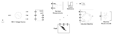
Figure 1: MATLAB Simulink^® SimScape model for an induction motor with a fault at the terminals.

TABLE I: Case Study Parameters

Subsystem	Parameter	Symbol	Value	Units
	Nominal Power	$P$	3.73	kW
	Voltage (line-line)	$V_{ll}$	460	V
	Frequency	$f$	60	Hz
	Pole Pairs	$P$	2
	Inertia	$J$	0.02	$\mathrm{kg\cdot m^{2}}$
Stator	Resistance	$R_{s}$	1.115	$\Omega$
Stator	Inductance	$L_{ls}$	5.974	mH
Rotor	Resistance	$R_{r}^{\prime}$	1.083	$\Omega$
Rotor	Inductance	$L_{lr}^{\prime}$	5.974	mH
Rotor	Mutual Inductance	$L_{m}$	203.7	mH
Load	Torque	$T_{m}$	50	$\mathrm{N\cdot m}$
Fault	Fault Resistance	$R_{f}$	5.0	$\Omega$
Fault	Ground Resistance	$R_{g}$	0.1	$\Omega$

The sequence of events in the simulation is as follows:

1. the motor is connected to power at $0~{}sec$,

2. the constant-torque load is activated at $3~{}sec$,

3. a fault is applied at $5~{}sec$, and

4. the fault is cleared at $5.25~{}sec$.

The following quantities are recorded during the simulation:

• line-ground voltage on each phase at the voltage source,

• current on each phase at the voltage source,

• mechanical torque drawn by the load, and

• rotor shaft speed.

For the voltage and current measurements, Park’s transformation was performed to produce the discretized set of observables in (28).

Four different scenarios were considered (Table II). The transformed measurements were down-sampled to a 100 Hz sample rate and applied to the DSE algorithm during the fault period.

TABLE II: Case Study Results

Case	Phasing	$\chi^{2}$ CDF
No Fault	–	0.988
Line-Ground Fault	AG	0.925
Line-Line Fault	AB	0.413
Three-Phase Ground Fault	ABCG	0.800

IV Experiment Results

Measured voltages and currents, for the four fault scenarios considered, are illustrated in Figs. 2 – 5. Applying the DSE algorithm during the fault period yields the Chi-Squared statistic in column 3 of Table II. Testing to a 95 % confidence interval allow for faulted conditions to be detected.

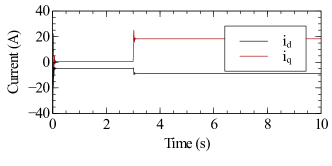
Figure 2: Measured voltage and current for unfaulted conditions.

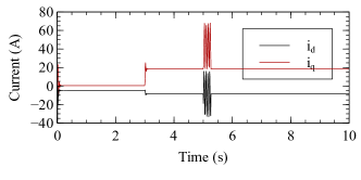
Figure 3: Measured voltage and current for a line-ground fault.

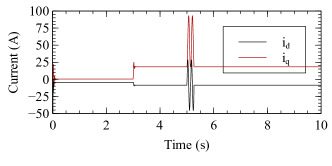
Figure 4: Measured voltage and current for a line-line fault.

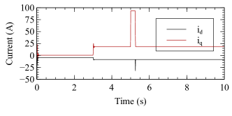
Figure 5: Measured voltage and current for a three-phase-ground fault.

V Conclusions

This work investigated the application of DSE for load bus protection with dynamic loads, in the case of a three-phase induction motor. Results suggest that DSE is a feasible method for protection under common fault types based on the ability of the DSE to accurately detect faults on the case study system with a confidence test.

As DSE is a generalisation of differential protection, it can be applied to a wide range of power conversion elements: not only to conventional elements such as transformers, transmission lines, and shunt capacitors, but to elements such as motor loads in microgrids as well. It is expected that this protection method can be applied to other forms of dynamic loads, such as single-phase induction motors or active rectifiers as well. Additionally, it is expected that this method could be extended to not only model individual loads, but to be representative of composite load models as well – along the lines of the WECC CMPLDW model – representing the dynamic behavior of the downstream radial portions of microgrids.

Future work will aim to investigate these above described other applications, in addition to the feasibility of applying DSE for load bus protection in a real-time implementations.

References

- [1] J. Duan et al. Distributed Control of Inverter-Interfaced Microgrids Based on Consensus Algorithm With Improved Transient Performance. IEEE Trans. Smart Grid, 10(2):1303–1312, Mar. 2019.
- [2] P. Aree. Accurate Initialization of Islanded Microgrid Including Induction Motor Load Using Unified Power-Flow Approach. Electrical Engineering, 103(6):3085–3096, Dec. 2021.
- [3] P. Krause et al. Analysis of Electric Machinery and Drive Systems. Somerset: Wiley, 3 edition, Jun. 2013.
- [4] P. F. Le Roux et al. Static and Dynamic Simulation of an Induction Motor Using Matlab/Simulink. Energies, 15(10), May 2022.
- [5] D. S. Brereton et al. Representation of Induction-Motor Loads During Power-System Stability Studies. IEEE Trans. Power App. Syst., 76(3):451–460, Apr. 1957.
- [6] N. Afrin et al. Impact of Induction Motor Load on the Dynamic Voltage Stability of Microgrid. In Proc. of the 2018 Australian & New Zealand Control Conference, 2018.
- [7] M. G. Ioannides. Design and Implementation of PLC-based Monitoring Control System for Induction Motor. IEEE Trans. Energy Convers., 19(3):469–476, 2004.
- [8] A. K. Barnes et al. Implementing Admittance Relaying for Microgrid Protection. In Proc. of the 2021 IEEE/IAS 57th Industrial and Commercial Power Systems Technical Conference, Apr. 2021.
- [9] M. Dewadasa et al. Line Protection in Inverter Supplied Networks. In Proc. of the 2008 Australasian Universities Power Engineering Conference, 2008.
- [10] S. Kar et al. Time-Frequency Transform-Based Differential Scheme for Microgrid Protection. IET Generation, Transmission & Distribution, 8(2):310–320, Feb. 2014.
- [11] J.-J. Huang. Adaptive Wide Area Protection of Power Systems. In Researchgate, 2004.
- [12] O. Vasios et al. A Dynamic State Estimation Based Centralized Scheme for Microgrid Protection. In Proc. of the 2018 North American Power Symposium, 2018.
- [13] A. K. Barnes et al. Dynamic State Estimation for Radial Microgrid Protection. In Proc. of the 2021 IEEE/IAS 57th Industrial and Commercial Power Systems Technical Conference, Apr. 2021.
- [14] M. Vanin et al. A Framework for Constrained Static State Estimation in Unbalanced Distribution Networks. IEEE Trans. Power Syst., 37(3):2075–2085, May 2022.
- [15] J. Zhao et al. Power System Dynamic State Estimation: Motivations, Definitions, Methodologies, and Future Work. IEEE Trans. Power Syst., 34(4):3188–3198, Jul. 2019.
- [16] Y. Liu et al. Dynamic State Estimation for Power System Control and Protection. IEEE Trans. Power Syst., 36(6), Nov. 2021.
- [17] S. Choi et al. Effective Real-Time Operation and Protection Scheme of Microgrids Using Distributed Dynamic State Estimation. IEEE Trans. Power Del., 32(1):504–414, Feb. 2017.
- [18] H. F. Albinali et al. Hidden Failure Detection Via Dynamic State Estimation in Substation Protection Systems. In Proc. of the 2017 Saudi Arabia Smart Grid, Dec. 2017.
- [19] A. K. Barnes et al. Dynamic State Estimation for Load Bus Protection on Inverter-Interfaced Microgrids. In Proc. of the 2022 IEEE PES/IAS PowerAfrica Conference, Aug. 2022.
- [20] E. Dehghanpour et al. A Protection System for Inverter Interfaced Microgrids. IEEE Trans. Power Del., Sep. 2021.
- [21] J. Zhao et al. Roles of Dynamic State Estimation in Power System Modeling, Monitoring and Operation. IEEE Trans. Power Syst., 36(3):2462–2472, May 2021.
- [22] J. Bezanson, S. Karpinski, V. B. Shah, and A. Edelman. Julia: A Fast Dynamic Language for Technical Computing. https://julialang.org/, 2012.
- [23] MathWorks. Matlab aysnchronous machine. https://www.mathworks.com/help/physmod/sps/powersys/ref/asynchronousmachine.html.
- [24] P. Kundur et al. Power System Stability and Control. McGraw-Hill, 1994.
- [25] H. F. Albinali et al. Dynamic State Estimation-Based Centralized Protection Scheme. In Proc. of the 2017 IEEE Manchester PowerTech, 2017.
- [26] JuliaDiff. Finitediff. https://github.com/JuliaDiff/FiniteDiff.jl.