Lifted Bregman Training of Neural Networks

Abstract

We introduce a novel mathematical formulation for the training of feed-forward neural networks with (potentially non-smooth) proximal maps as activation functions. This formulation is based on Bregman distances and a key advantage is that its partial derivatives with respect to the network’s parameters do not require the computation of derivatives of the network’s activation functions. Instead of estimating the parameters with a combination of first-order optimisation method and back-propagation (as is the state-of-the-art), we propose the use of non-smooth first-order optimisation methods that exploit the specific structure of the novel formulation. We present several numerical results that demonstrate that these training approaches can be equally well or even better suited for the training of neural network-based classifiers and (denoising) autoencoders with sparse coding compared to more conventional training frameworks.

Keywords: Lifted network training, distributed optimisation, Bregman distances, sparse autoencoder, denoising autoencoder, classification, compressed sensing

1 Introduction

Deep neural networks (DNNs) are extremely popular choices of model functions for a great variety of machine learning problems (cf. Goodfellow et al. (2016)). The predominant strategy for training DNNs is to use a combination of gradient-based minimisation algorithm and the back-propagation algorithm (Rumelhart et al., 1986). Thanks to modern automatic differentiation frameworks, this approach is easy to implement and yields satisfactory results for a great variety of machine learning applications. However, this approach does come with numerous drawbacks. First of all, many common activation functions in neural network architectures are not differentiable, which means that subgradient- instead of gradient-based algorithms are required. And even though there are mathematical justifications for such an approach (cf. Bolte and Pauwels (2020)), subgradient-based methods have the disadvantage of inferior convergence rates over other non-smooth optimisation methods like proximal gradient descent (cf. Teboulle (2018)). Another drawback is that back-propagation suffers from vanishing gradient problems (Erhan et al., 2009), where gradients of loss functions with respect to the parameters of early network layers become vanishingly small, which renders the use of gradient-based minimisation methods ineffective. While the use of non-saturating activation functions and the introduction of skip-connections to network architectures have been proposed to mitigate vanishing gradient problems, achieving state-of-the-art performance still requires meticulous hyper-parameter tuning and good initialisation strategies. Another issue of the back-propagation algorithm is that it is sequential in nature, which makes it difficult to distribute the computation of the network parameters across multiple workers efficiently. As a consequence of the aforementioned issues, numerous distributed optimisation approaches have been proposed as alternatives to gradient-based training in combination with back-propagation in recent years (Carreira-Perpinan and Wang, 2014; Taylor et al., 2016; Zhang and Brand, 2017; Askari et al., 2018; Li et al., 2019; Zach and Estellers, 2019; Gu et al., 2020; Høier and Zach, 2020). However, many of these approaches still suffer from limitations such as differentiating non-differentiable activation functions (Carreira-Perpinan and Wang, 2014), recovering affine-linear networks (Askari et al., 2018), or overly restrictive assumptions (Li et al., 2019; Gu et al., 2020).

In this work, we propose a distributed optimisation framework for the training of parameters of feed-forward neural networks that does not require the differentiation of activation functions, that does train truly non-linear DNNs, that can be optimised with a variety of deterministic and stochastic first-order optimisation methods and that does come with extensive mathematical foundations. The proposed approach is a generalisation of the Method of Auxiliary Coordinates with Quadratic Penalty (Carreira-Perpinan and Wang, 2014); instead of quadratic penalty functions, we propose to use a novel penalty function based on a special type of Bregman distance, respectively Bregman divergence (Bregman, 1967).

The main contributions of this paper are: 1) the proposal of a new loss function that, when differentiated with respect to its second argument, does not require the differentiation of an activation function, 2) its use as a penalty function within the method of auxiliary coordinates, 3) a detailed mathematical analysis of the new loss function, 4) the proposal of a variety of different deterministic and stochastic iterative minimisation algorithms for the empirical risk minimisation of DNNs, 5) the comparison of these iterative minimisation algorithms to more conventional approaches such as stochastic gradient descent and back-propagation, 6) the show-casing of the proposed approach for the training of (denoising) autoencoders with sparse codes, and 7) a demonstration that contrary to wide-spread belief, expressive feed-forward networks can overfit to training data without generalising well when non-standard optimisation methods are being used.

The paper is organised as follows. We describe the state-of-the-art approach of training neural networks with gradient-based algorithms and back-propagation, before we provide an overview over recent developments in distributed optimisation methods for the training of DNNs in Section 2. In Section 3, we introduce our proposed lifted Bregman framework. We first establish mathematical foundations, before we define the Bregman loss function that replaces the quadratic penalty function in the method of auxiliary coordinates, and verify a whole range of mathematical properties of this loss function that guarantee the advantages over other approaches. In Section 4, we provide an overview over a range of deterministic and stochastic optimisation approaches that are able to computationally solve the lifted Bregman training problem thanks to results provided in Section 3. We also discuss suitable regularisation strategies for the regularisation of network parameters and outputs of hidden network layers. In Section 5, we discuss the example problems of classification, data compression and denoising. For the latter two, we introduce a regularised empirical risk minimisation approach that will produce autoencoders with sparse codes. In Section 6, we provide numerical results for the example problems described in Section 5 and extensive comparisons to other minimisation approaches. In Section 7, we conclude with a summary of the findings and an outlook of future developments.

2 Training neural networks

Traditionally, the predominant strategy for training neural networks is the use of a gradient-based minimisation algorithm in combination with the back-propagation algorithm. Alternatively, distributed optimisation techniques for training neural networks have received growing attention in recent years (cf. Carreira-Perpinan and Wang (2014)). In the following sections, we revisit the notion of feed-forward neural networks before we summarise the classical approach of gradient-based training and back-propagation. We then discuss distributed optimisation and lifted training strategies.

2.1 Feed-forward neural networks

A feed-forward neural network $\mathcal{N}:\mathbb{R}^{n}\times\mathcal{P}\rightarrow\mathbb{R}^{m}$ with $L$ layers can be defined as the composition of parametrised functions of the form

$$\mathcal{N}(x,\mathbf{\Theta})=\sigma_{L}(f(\sigma_{L-1}(f(\ldots\sigma_{1}(f(x_{1},\Theta_{1}))\ldots)),\Theta_{L})),$$ (1)

for given input data $x\in\mathbb{R}^{n}$ and parameters $\mathbf{\Theta}\in\mathcal{P}$. Here $\{\sigma_{l}\}_{l=1}^{L}$ denotes the collection of nonlinear activation functions and $f$ denotes a generic function parametrised by parameters $\{\Theta_{l}\}_{l=1}^{L}$. To ease the notation, we use $\mathbf{\Theta}$ to denote $\{\Theta_{l}\}_{l=1}^{L}$. As an example, a rectified linear unit (ReLU) (Nair and Hinton, 2010) can be constructed via the composition of $\sigma_{l}(\cdot):=\text{max}(0,\cdot)$ and $f(x,\Theta_{l})=W^{\top}_{l}x+b_{l}$ for $\Theta_{l}=(W_{l},b_{l})$, where the matrix $W_{l}$ is usually referred to as the weights and the vector $b_{l}$ as the bias term of layer $l$. We refer to the output of the neural network model as $\hat{y}$, i.e. $\hat{y}:=\mathcal{N}(x,\mathbf{\Theta})$.

2.2 Training feed-forward networks with first-order methods and back-propagation

Estimating parameters $\mathbf{\Theta}$ of a feed-forward network in the supervised learning setting is usually framed as the minimisation of an empirical risk of the form

$$\min_{\mathbf{\Theta}}\frac{1}{s}\sum_{i=1}^{s}\ell(y^{i},\hat{y}^{i})\,,$$ (2)

where $\ell$ is a chosen data error term pertaining to the learning task (usually referred to as loss), while $\{(x^{i},y^{i})\}_{i=1}^{s}$ denotes the $s$ pairs of input and output samples that have to be provided a-priori. A standard computational approach to solve (2) are (sub-)gradient-based algorithms such as (sub-)gradient descent and stochastic variants of it. Gradient descent for solving (2) reads

$$\mathbf{\Theta}^{k+1}=\mathbf{\Theta}^{k}-\tau_{\mathbf{\Theta}}\nabla_{\mathbf{\Theta}}\left(\frac{1}{s}\sum_{i=1}^{s}\ell(y^{i},\mathcal{N}(x^{i},\mathbf{\Theta}^{k}))\right)\,,$$ (3)

for $k\in\mathbb{N}$, a step-size parameter $\tau_{\mathbf{\Theta}}>0$ and initial parameters $\mathbf{\Theta}^{0}$. The evaluation of the gradient $\nabla_{\mathbf{\Theta}}\left(\frac{1}{s}\sum_{i=1}^{s}\ell(y^{i},\mathcal{N}(x^{i},\mathbf{\Theta}^{k}))\right)$ is computed with the back-propagation (cf. Rumelhart et al. (1986)), which is summarised in Algorithm 2 in Appendix A. As pointed out in LeCun et al. (1988), the back-propagation algorithm can also be deduced from a Lagrangian formulation of (2), where solving the corresponding optimality system leads to the individual steps in the back-propagation algorithm. For each pair of data samples $(x^{i},y^{i})$ we can define

$$x_{l}^{i}=\sigma_{l}(f(x_{l-1}^{i},\Theta_{l}))\qquad\text{for}\qquad l=1,\ldots,L\,,$$ (4)

as the so-called activation variables with initial value $x_{0}^{i}=x^{i}$. Further, we use $z_{l}^{i}$ to denote transformed input variables by

$$z_{l}^{i}=f(x_{l-1}^{i},\Theta_{l})\qquad\text{for}\qquad l=1,\ldots,L\,.$$

To ease notation, we introduce $\mathbf{X}=\{x_{l}^{i}\}_{l=1,\ldots,L}^{i=1,\ldots,s}$ and $\mathbf{Z}=\{z_{l}^{i}\}_{l=1,\ldots,L}^{i=1,\ldots,s}$ to denote the two groups of auxiliary variables. Having introduced $\mathbf{X}$ and $\mathbf{Z}$, we can write the minimisation problem (2) in the following equivalent constrained form:

$$\begin{split}&\text{\;\;\;\;\; }\min_{\mathbf{\Theta},\mathbf{X},\mathbf{Z}}\frac{1}{s}\sum_{i=1}^{s}\ell(y^{i},x_{L}^{i})\\ &\text{\;\;\;\;\;\;\;s.t. }z_{l}^{i}=f(x_{l-1}^{i},\Theta_{l})\,\text{ for $l=1,\ldots,L$}\,,\\ &\text{\;\;\;\;\;\;\;s.t. }x_{l}^{i}=\sigma_{l}(f(x_{l-1}^{i},\Theta_{l}))\,\text{ for $l=1,\ldots,L$}\,.\end{split}$$ (5)

A derivation of Algorithm 2 from the Lagrangian formulation of (5) is included in Appendix A.

Despite its popularity for training neural networks, the approach of using (sub-)gradient based methods such as (3) in combination with Algorithm 2 nevertheless suffers from some some drawbacks. Two of the major problems are the vanishing and exploding gradient issues, where the gradients either decrease to vanishingly small values or increase to very large values, which causes major problems for the computation of (3) (cf. Glorot and Bengio (2010); Bengio et al. (1994)).

A third issue is that the back-propagation algorithm is sequential in nature and computation of individual partial derivatives cannot easily be distributed. A fourth drawback is that while it is easy to generalise gradient-based algorithms to proximal gradient methods that can handle non-smooth functions acting on the network parameters, it is less straight-forward to generalise these techniques so that they can handle non-smooth functions acting on the activation variables or the transformed input variables without using subgradients.

These drawbacks and limitations of the combination of (sub-)gradient based-methods and back-propagation have motivated research to seek for alternative training methods for DNNs. In the next section, we will summarise some of these alternatives.

2.3 Distributed optimisation approaches

Learning network parameters via distributed optimisation has been given much attention in recent years (Carreira-Perpinan and Wang, 2014; Taylor et al., 2016; Zhang and Brand, 2017; Askari et al., 2018; Li et al., 2019; Zach and Estellers, 2019; Gu et al., 2020). In these works, the overall Learning Problem (2) is reformulated to Problem (5).

This constrained optimisation Problem (5) can further be relaxed by replacing the constraints for the activation variables with penalty terms in the objective function. Solving each layer-wise sub-problem can then be performed independently, which allows for distributed optimisation methods to be utilised. This attempt has mainly been approached from two directions: by using quadratic penalties (Carreira-Perpinan and Wang, 2014; Taylor et al., 2016) or by framing activation functions as orthogonal projections on convex sets of constraints (Zhang and Brand, 2017; Askari et al., 2018; Li et al., 2019; Zach and Estellers, 2019; Gu et al., 2020).

2.3.1 Method of Auxiliary Coordinates with Quadratic Penalty (MAC-QP)

The work of Carreira-Perpinan and Wang (2014) is among the earliest to look into the quadratic penalty approach, where the authors propose the Method of Auxiliary Coordinates (MAC) that relaxes the Learning Problem (2) by replacing the constraints $x_{l}^{i}=\sigma_{l}(f(x_{l-1}^{i},\Theta_{l}))$ with a Quadratic Penalty (QP) objective where the corresponding minimisation problem reads

$$\min_{\mathbf{X},\mathbf{\Theta}}\frac{1}{s}\sum_{i=1}^{s}\left[\ell(y^{i},f(x_{L-1}^{i},\Theta_{L}))+\sum_{l=1}^{L-1}\|x^{i}_{l}-\sigma_{l}(f(x_{l-1}^{i},\Theta_{l}))\|_{2}^{2}\right]\,.$$ (6)

If we consider the special case of affine-linear functions $f(x_{l-1},\Theta_{l})=W_{l}^{\top}x_{l-1}+b_{l}$, then for $s=1$ and a single training pair of samples $x$ and $y$ the optimality condition w.r.t the bias parameter $b_{l}$ reads

$$0=(x_{l}-\sigma_{l}(W_{l}^{\top}x_{l-1}+b_{l}))\sigma_{l}^{\prime}(W_{l}^{\top}x_{l-1}+b_{l})\,.$$

Whenever $\sigma_{l}^{\prime}(W_{l}^{\top}x_{l-1}+b_{l})\neq 0$, this automatically implies

$$x_{l}=\sigma_{l}(W_{l}^{\top}x_{l-1}+b_{l})\,,$$

ensuring that a critical point satisfies (4). Following the MAC-QP approach, minimisation of network parameters can easily be distributed with the right choice of optimisation method. However, minimising the MAC-QP objective with gradient-based fist-order optimisation methods still requires the differentiation of the activation functions. This is different for lifted training approaches that we briefly discuss in the next section.

2.3.2 Lifted training approach

The second line of work to approach Problem (5) is motivated by the observation that the ReLU activation function $\sigma(z,0)=\max(z,0)$ itself can be viewed as the solution to a constrained minimisation problem. More specifically, in the work of Zhang and Brand (2017), the authors characterise the activated output of the ReLU activation function $\sigma_{l}(W_{l}^{\top}x_{l-1}+b_{l})$ as

$$x_{l} =\sigma_{l}(W_{l}^{\top}x_{l-1}+b_{l})$$

$$=\operatorname*{\arg\min}_{x\geq 0}\|x-(W_{l}^{\top}x_{l-1}+b_{l})\|_{2}^{2}\,\,.$$

This implies that $x_{l}$ is the vector closest to $W_{l}^{\top}x_{l-1}+b_{l}$ that lies in the non-negative orthant.

In the classical lifted approach (Askari et al., 2018), Problem (5) is consequently approximated with

$$\min_{\mathbf{\Theta},\{x_{l}^{i}\in\mathbb{R}_{+}^{n}\}_{l=1}^{L-1}}\frac{1}{s}\sum_{i=1}^{s}\left[\ell(y^{i},f(x^{i}_{L-1},\Theta_{L}))+\sum_{l=1}^{L-1}\|x^{i}_{l}-f(x^{i}_{l-1},\Theta_{l})\|_{2}^{2}\right]\,,$$ (7)

where $\{x_{l}^{i}\in\mathbb{R}_{+}^{n}\}_{l=1}^{L-1}$ denotes that the activation variables across layers $l=1,\ldots,L-1$ for each sample $i$ lie in the non-negative orthant, i.e. $\mathbb{R}_{+}^{n}:=\{v\in\mathbb{R}^{n}\,|v_{j}\geq 0,\;\forall\,j\in\{1\ldots n\}\}$. This approach is often referred to as the “lifted” approach because the search space for network parameters is lifted to become a higher dimensional space that now also includes auxiliary variables. However, this “lifting” is obviously also present in MAC-QP.

Even though the overall learning problem (7) is not convex, each sub-problem is convex in each individual variable when keeping all other variables fixed. Individual updates are also relatively easy to compute using orthogonal projections onto the non-negative orthant. In terms of distributing the computation of parameters, this approach also enjoys the same benefits that the MAC-QP scheme enjoys. However, one major limitation that this approach suffers from is that it does not solve the original Problem (2), but essentially trains an affine-linear network (cf. Zach and Estellers (2019)). This restriction can be shown by examining the optimality system. Consider the case with $s=1$ and one single training sample pair $(x,y)$, then the optimality condition of (7) with respect to parameters $b_{l}$ reads

$$(W_{l}^{\top}x_{l-1}+b_{l}-x_{l})=0\qquad\Longrightarrow\qquad x_{l}=W_{l}^{\top}x_{l-1}+b_{l}\,\,.$$ (8)

Despite this major limitation this approach has been considered for computing initialisations of network parameters for other optimisation algorithms (Li et al., 2019; Zach and Estellers, 2019).

3 Lifted Bregman training framework

Building upon the previous approaches, we introduce a lifted Bregman framework for the training of feed-forward networks. This framework will fix the aforementioned issues and 1) be capable of recovering a network with nonlinear activation functions, while 2) taking partial derivatives with respect to network parameters will not require computing derivatives of the activation functions.

Our approach differs from Problem (6) and Problem (7) in the sense that instead of penalising the quadratic Euclidean norm of the nonlinear constraint $x_{l}^{i}=\sigma_{l}\left(f(x_{l-1}^{i},\Theta_{l})\right)$ we propose an alternative penalisation. From now on we assume that the activation functions $\sigma_{l}$ that we consider come from the large class of proximal maps.

Definition 1 (Proximal map)

The proximal map $\sigma:\mathbb{R}^{n}\rightarrow\textnormal{dom}(\Psi)\subset\mathbb{R}^{n}$ of a proper, lower semi-continuous and convex function $\Psi:\mathbb{R}^{n}\rightarrow\mathbb{R}\cup\{\infty\}$ is defined as

$$\sigma(z)=\textnormal{prox}_{\Psi}(z):=\operatorname*{\arg\min}_{u\in\mathbb{R}^{n}}\left\{\frac{1}{2}\|u-z\|^{2}+\Psi(u)\right\}\,.$$ (9)

Example 1 (Proximal maps)

There are numerous examples of commonly used activation functions in deep learning that are also proximal maps (cf. Zhang and Brand (2017); Li et al. (2019); Combettes and Pesquet (2020); Hasannasab et al. (2020)). We give the following four examples. The first one is the rectifier or ramp function that is also known as Rectified Linear Unit (ReLU) (cf. Nair and Hinton (2010)). The ramp function is a special case of Definition 1 for the characteristic function over the non-negative orthant, i.e.

$$\Psi(u):=\begin{cases}0&u\in[0,\infty)^{n}\\ \infty&\text{otherwise}\end{cases}\qquad \implies\qquad\sigma(z)_{j}=\max(0,z_{j})\,,\;\forall j\in\{1,\ldots,n\}\,.$$

The well-known soft-thresholding function is a proximal map for a positive multiple of the one-norm, i.e.

$$\Psi(u):=\alpha\|u\|_{1}\qquad \implies\qquad\sigma(z)_{j}=\begin{cases}z_{j}-\alpha&z_{j}>\alpha\\ 0&|z_{j}|\leq\alpha\\ z_{j}+\alpha&z_{j}<-\alpha\end{cases}\,,\;\forall j\in\{1,\ldots,n\}\,,$$

for $\alpha>0$. Common smooth activation functions like the hyperbolic tangent can also be framed as proximal maps. The hyperbolic tangent can be recovered by choosing the characteristic function

$$\Psi(u):=\begin{cases}u\tanh^{-1}(u)+\frac{1}{2}\left(\log(1-u^{2})-u^{2}\right)&|u|<1\\ \infty&\text{otherwise}\end{cases}\qquad\implies\qquad\sigma(z)=\tanh(z)\,.$$

All previous examples were separable activation functions. Our final example is the non-separable softmax activation function, which we can obtain as a proximal map for the characteristic function

$$\Psi(u) :=\begin{cases}\sum_{j=1}^{n}\left[u_{j}\log(u_{j})-\frac{1}{2}u_{j}^{2}\right]&u_{j}\geq 0\,,\,\sum_{j=1}^{n}u_{j}=1\\ \infty&\text{otherwise}\end{cases}$$

$$\implies\qquad\sigma(z)_{j} =\frac{\exp(z_{j})}{\sum_{k=1}^{n}\exp(z_{k})}\,,\;\forall j\in\{1,\ldots,n\}\,.$$

In Figure 1, we show visualisations of the above mentioned proximal activation functions.

Figure 1: This figure shows example activation functions that are also proximal maps. From left to right on the top row are the ReLU activation function, the soft-thresholding activation function (threshold value $\alpha=0.5$) and the hyperbolic tangent activation function respectively. The bottom two figures visualise components of the softmax activation function for the case of $n=2$.

For convex functions $\Psi$, the following remark gives an alternative characterisation of the proximal map.

Remark 2

Note that an equivalent characterisation of the proximal map $\sigma$ is

$$z-\sigma(z)\in\partial\Psi(\sigma(z))\,,$$

as a consequence of Fermat’s theorem. Here $\partial\Psi$ denotes the subdifferential of $\Psi$.

With the help of Remark 2, we discover that $x_{l}=\sigma(f(x_{l-1},\Theta_{l}))$ can also be written as

$$f(x_{l-1},\Theta_{l})-x_{l}\in\partial\Psi(x_{l})\,,\qquad\text{respectively, }\qquad f(x_{l-1},\Theta_{l})\in\partial\left(\frac{1}{2}\|\cdot\|^{2}+\Psi\right)(x_{l})\,,$$ (10)

where the second inclusion follows from (Ekeland and Temam, 1999, Chapter 1, Section 5, Proposition 5.6). We want to briefly recall the concept of Fenchel duality before we proceed.

Definition 3 (Fenchel conjugate)

For a proper, convex and semi-continuous function $F$ its convex- or Fenchel-conjugate $F^{\ast}$ is defined as

$$F^{\ast}(y):=\sup_{x}\left\{\langle x,y\rangle-F(x)\right\}\,.$$

The following neat equivalence for inclusion (10) forms the basis for our new penalisation term.

Lemma 4 (Subdifferential characterisation)

Suppose the function $\Psi:\mathbb{R}^{n}\rightarrow\mathbb{R}\cup\{\infty\}$ is a proper, lower semi-continuous and convex function. Then the inclusion $z\in\partial\left(\frac{1}{2}\|\cdot\|^{2}+\Psi\right)(x)$ is equivalent to

$$\frac{1}{2}\|x\|^{2}+\Psi(x)+\left(\frac{1}{2}\|\cdot\|^{2}+\Psi\right)^{\ast}\left(z\right)=\langle x,z\rangle\,.$$ (11)

Here, $\left(\frac{1}{2}\|\cdot\|^{2}+\Psi\right)^{\ast}$ denotes the Fenchel conjugate of $\frac{1}{2}\|\cdot\|^{2}+\Psi$.

A proof for this lemma can be found in (Rockafellar, 1970, Theorem 23.5), where a more general result is proven. Now, instead of enforcing (11) as a hard constraint, we define the penalisation function

$$B_{\Psi}(x,z):=\frac{1}{2}\|x\|^{2}+\Psi(x)+\left(\frac{1}{2}\|\cdot\|^{2}+\Psi\right)^{\ast}\left(z\right)-\langle x,z\rangle\,,$$ (12)

and replace the squared Euclidean norm in (7) with it, which results in the unconstrained optimisation problem

$$\min_{\mathbf{\Theta},\mathbf{X}}\sum_{i=1}^{s}\left[\ell\left(y^{i},x_{L}^{i}\right)+\sum_{l=1}^{L-1}\,\lambda_{l}B_{\Psi}\left(x_{l}^{i},f(x_{l-1}^{i},\Theta_{l})\right)\right]\,.$$ (13)

for positive scalars $\{\lambda_{l}\}_{l=1}^{L-1}$.

We name this penalisation function $B_{\Psi}(x,z)$ Bregman loss, as we are going to show that it belongs to the family of generalised Bregman distances (Bregman, 1967; Kiwiel, 1997). In the following sections, we provide a more detailed analysis of the Bregman loss and show how it can improve the classical lifted training approach and overcome its limitations.

3.1 The Bregman loss function

We want to verify that the proposed Bregman loss function (12) is a non-negative generalised Bregman distance (Bregman, 1967; Kiwiel, 1997) and satisfies some advantageous properties compared to the mean-squared error loss used in (7).

The generalised Bregman distance induced by a proper, convex and lower semi-continuous function $\Phi$ is defined as follows.

Definition 5 (Generalised Bregman distance)

The generalised Bregman distance of a proper, lower semi-continuous and convex function $\Phi$ is defined as

$$D_{\Phi}^{q(v)}(u,v) :=\Phi(u)-\Phi(v)-\langle q(v),u-v\rangle\,,$$

Here, $q(v)\in\partial\Phi(v)$ is a subgradient of $\Phi$ at argument $v\in\mathbb{R}^{n}$.

For examples of (generalised) Bregman distances we refer the reader to Bregman (1967); Censor and Lent (1981); Kiwiel (1997); Burger (2016); Benning and Riis (2021).

We now want to verify that the function (12) is a Bregman distance in the sense of Definition 5. This directly follows from (11), as we can replace $\left(\frac{1}{2}\|\cdot\|^{2}+\Psi\right)^{\ast}\left(z\right)$ in (12) with $\langle\sigma(z),z\rangle-\frac{1}{2}\|\sigma(z)\|^{2}-\Psi(\sigma(z))$ because of $z\in\partial(\frac{1}{2}\|\cdot\|^{2}+\Psi)(\sigma(z))$. We then obtain

$$B_{\Psi}(x,z) =\frac{1}{2}\|x\|^{2}+\Psi(x)+\left(\frac{1}{2}\|\cdot\|^{2}+\Psi\right)^{\ast}\left(z\right)-\langle x,z\rangle\,,$$

$$=\frac{1}{2}\|x\|^{2}+\Psi(x)-\frac{1}{2}\|\sigma(z)\|^{2}-\Psi(\sigma(z))+\langle\sigma(z),z\rangle-\langle x,z\rangle\,,$$

$$=\frac{1}{2}\|x\|^{2}+\Psi(x)-\left(\frac{1}{2}\|\sigma(z)\|^{2}+\Psi(\sigma(z))\right)-\langle z,x-\sigma(z)\rangle\,$$

$$=D_{\frac{1}{2}\|\cdot\|^{2}+\Psi}^{z}(x,\sigma(z))\,.$$

The last equality is correct because of $z\in\partial\left(\frac{1}{2}\|\cdot\|^{2}+\Psi\right)(\sigma(z))$, which is equivalent to $z-\sigma(z)\in\partial\Psi(\sigma(z))$, respectively $\sigma(z)=\textnormal{prox}_{\Psi}(z)$ as pointed out in Remark 2. Since this is true by definition of $\sigma$, we have established that $B_{\Psi}(x,z)$ is a Bregman distance. Since Bregman distances are non-negative, this automatically implies non-negativity of $B_{\Psi}(x,z)$ for all arguments $x,z$, but we easily get a better lower bound if we split the Bregman distance, i.e.

$$B_{\Psi}(x,z) =D_{\frac{1}{2}\|\cdot\|^{2}+\Psi}^{z}(x,\sigma(z))=D_{\frac{1}{2}\|\cdot\|^{2}}^{\sigma(z)}(x,\sigma(z))+D_{\Psi}^{z-\sigma(z)}(x,\sigma(z))\,,$$

$$=\frac{1}{2}\|x-\sigma(z)\|^{2}+D_{\Psi}^{z-\sigma(z)}(x,\sigma(z))\geq\frac{1}{2}\|x-\sigma(z)\|^{2}\,,$$

which we capture with the following corollary.

Corollary 6

The loss function $B_{\Psi}$ as defined in (12) is a Bregman distance and bounded from below by $\frac{1}{2}\|x-\sigma(z)\|^{2}$.

Proof  This follows from the fact that $D_{\Psi}^{z-\sigma(z)}(x,\sigma(z))$ is a valid generalised Bregman distance, because of $z-\sigma(z)\in\partial\Psi(\sigma(z))$ by definition of $\sigma$. Hence, $D_{\Psi}^{z-\sigma(z)}(x,\sigma(z))\geq 0$, which concludes the proof.  

Hence, we can characterise the exact discrepancy between $B_{\Psi}(x,z)$ and $\frac{1}{2}\|x-\sigma(z)\|^{2}$ in terms of $D_{\Psi}^{z-\sigma(z)}(x,\sigma(z))$, which means we establish

$$B_{\Psi}(x,z) =\frac{1}{2}\|x-\sigma(z)\|^{2}+\Psi(x)-\Psi(\sigma(z))-\langle z-\sigma(z),x-\sigma(z)\rangle\,,$$

$$=\frac{1}{2}\|x-\sigma(z)\|^{2}+\Psi(x)+\Psi^{\ast}(z-\sigma(z))-\langle x,z-\sigma(z)\rangle\,,$$ (14)

We can further simplify this term with the help of the Moreau identity.

Theorem 7 (Moreau identity (Moreau, 1962))

Suppose $\Psi:\mathbb{R}^{n}\rightarrow\mathbb{R}\cup\{\infty\}$ is a proper, convex and lower-semicontinuous function with Fenchel conjugate $\Psi^{\ast}$, and we have $\sigma(x):=\textnormal{prox}_{\Psi}(x)$ and $\sigma^{\ast}(x):=\textnormal{prox}_{\Psi}(x)$. Then

$$x=\sigma(x)+\sigma^{\ast}(x)$$

holds true for all $x\in\mathbb{R}^{n}$.

Hence, with Theorem 7, we can rewrite (14) to

$$B_{\Psi}(x,z)=\frac{1}{2}\|x-\sigma(z)\|^{2}+\Psi(x)+\Psi^{\ast}(\sigma^{\ast}(z))-\langle x,\sigma^{\ast}(z)\rangle\,.$$

If we define $E_{z}(x):=\frac{1}{2}\|x-z\|^{2}+\Psi(x)$ as the function for which we have $\sigma(z)=\textnormal{prox}_{\Psi}(z)=\operatorname*{\arg\min}_{x}E_{z}(x)$ and consequently $0\in\partial E_{z}(\sigma(z))$, we can further conclude

$$B_{\Psi}(x,z) =\frac{1}{2}\|x-\sigma(z)\|^{2}+\Psi(x)-\Psi(\sigma(z))-\langle z-\sigma(z),x-\sigma(z)\rangle\,,$$

$$=\frac{1}{2}\|x\|^{2}+\Psi(x)-\langle x,z\rangle+\frac{1}{2}\|\sigma(z)\|^{2}-\Psi(\sigma(z))+\langle z-\sigma(z),\sigma(z)\rangle\,,$$

$$=\frac{1}{2}\|x-z\|^{2}+\Psi(x)-\frac{1}{2}\|z\|^{2}-\frac{1}{2}\|\sigma(z)\|^{2}-\Psi(\sigma(z))+\langle z,\sigma(z)\rangle\,,$$

$$=\frac{1}{2}\|x-z\|^{2}+\Psi(x)-\frac{1}{2}\|\sigma(z)-z\|^{2}-\Psi(\sigma(z))\,,$$

$$=E_{z}(x)-E_{z}(\sigma(x))=D_{E_{z}}^{0}(x,\sigma(x))\,,$$

which is an alternative characterisation that is a valid Bregman distance because $0\in\partial E_{z}(\sigma(z))$ is a valid subgradient of $E_{z}$ at $\sigma(z)$. This characterisation nicely links to recent work in parametric majorisation for data-driven energy minimisation methods (Geiping and Moeller, 2019).

What makes the loss function (12) truly special, however, is its gradient with respect to its second argument.

Lemma 8 (Gradient of (12) with respect to second argument)

Suppose $\Psi:\mathbb{R}^{n}\rightarrow\mathbb{R}\cup\{\infty\}$ is a proper, convex and lower semi-continuous function with proximal map $\sigma:=\textnormal{prox}_{\Psi}$. Then the gradient of $B_{\Psi}(x,z)$ as defined in (12) with respect to its second argument, i.e. $\nabla_{2}B_{\Psi}(x,z)$, is

$$\nabla_{2}B_{\Psi}(x,z)=\sigma(z)-x\,,$$

for all $x\in\textnormal{dom}(\Psi)$.

Proof  Note that the term $\frac{1}{2}\|x\|^{2}+\Psi(x)$ in (12) is constant with respect to the argument $z$ and bounded because of $x\in\textnormal{dom}(\Psi)$, which implies

$$\nabla_{2}B_{\Psi}(x,z)=\nabla_{z}\left[\left(\frac{1}{2}\|\cdot\|^{2}+\Psi\right)^{\ast}(z)-\langle x,z\rangle\right]$$

for fixed $x$. The gradient of $\langle x,z\rangle$ with respect to the second argument $z$ is simply $x$; hence, what remains to be shown is that

$$\nabla\left(\frac{1}{2}\|\cdot\|^{2}+\Psi\right)^{\ast}(z)=\sigma(z)\,.$$ (15)

Since $\Psi$ is proper, convex and lower semi-continuous, the Fenchel conjugate $(\frac{1}{2}\|\cdot\|^{2}+\Psi)^{\ast}(z)=\sup_{x}\langle x,z\rangle-\frac{1}{2}\|x\|^{2}-\Psi(x)$ of $\frac{1}{2}\|\cdot\|^{2}+\Psi$ is well-defined and the supremum over $\langle z,x\rangle-\frac{1}{2}\|x\|^{2}-\Psi(x)$ is attained. More importantly, we have

$$\left(\frac{1}{2}\|\cdot\|^{2}+\Psi\right)^{\ast}(z) =\sup_{x}\langle x,z\rangle-\frac{1}{2}\|x\|^{2}-\Psi(x)\,,$$

$$=\frac{1}{2}\|z\|^{2}+\sup_{x}-\frac{1}{2}\|x-z\|^{2}-\Psi(x)\,,$$

$$=\frac{1}{2}\|z\|^{2}-\inf_{x}\left\{\frac{1}{2}\|x-z\|^{2}+\Psi(x)\right\}\,.$$

We know that $\sigma(z)=\textnormal{prox}_{\Psi}(z)=\operatorname*{\arg\min}_{x}\left\{\frac{1}{2}\|x-z\|^{2}+\Psi(x)\right\}$, which implies $x=\sigma(z)$ and

$$\left(\frac{1}{2}\|\cdot\|^{2}+\Psi\right)^{\ast}(z) =\frac{1}{2}\|z\|^{2}-\frac{1}{2}\|\sigma(z)-z\|^{2}-\Psi(\sigma(z))\,.$$

The quantity $M(z):=\frac{1}{2}\|\sigma(z)-z\|^{2}+\Psi(\sigma(z))$ is the Moreau-Yosida regularisation of $\Psi$, see (Moreau, 1965; Yosida, 1964), for which we know that its gradient is $\nabla M(z)=z-\textnormal{prox}_{\Psi}(z)=z-\sigma(z)$, cf. (Bauschke et al., 2011, Proposition 12.30). The gradient of $\frac{1}{2}\|z\|^{2}$ with respect to $z$ is simply $z$, which is why we have verified (15).  

Remark 9

Note that $\nabla_{2}B_{\Psi}(x,z)$ may be unbounded from below, which implies that $\nabla_{2}B_{\Psi}(x,z)$ may never be equal to zero for some choices of $x$. More precisely, $\nabla_{2}B_{\Psi}(x,z)=0$ is equivalent to $z-x\in\partial\Psi(x)$, which requires $\partial\Psi(x)\neq\emptyset$. Hence, if $x$ is chosen such that $\partial\Psi(x)=\emptyset$, we can never guarantee $\nabla_{2}B_{\Psi}(x,z)=0$. A simple example is $\Psi(x)=\chi_{\geq 0}(x)$ with negative argument $x$. In that case, there obviously cannot exist an element $z$ such that $\sigma(z)=\max(z,0)=x$ holds true because $\max(z,0)\geq 0$ while $x<0$.

We summarise all previous findings in the following theorem.

Theorem 10 (Bregman loss function)

The Bregman loss function as defined in (12) satisfies the following properties.

1. $B_{\Psi}(x,z)=E_{z}(x)-E_{z}(\sigma(z))$.

2. $B_{\Psi}(x,z)=D_{\frac{1}{2}\|\cdot\|^{2}+\Psi}^{z}(x,\sigma(z))$.

3. $B_{\Psi}(x,z)=\frac{1}{2}\|x-\sigma(z)\|^{2}+D_{\Psi}^{z-\sigma(z)}(x,\sigma(z))\geq\frac{1}{2}\|x-\sigma(z)\|^{2}$.

4. $B_{\Psi}(x,z)=\frac{1}{2}\|x-\sigma(z)\|^{2}+\Psi(x)-\Psi(\sigma(z))-\langle z-\sigma(z),x-\sigma(z)\rangle$.

5. For fixed first argument $x$, the function $B_{\Psi}$ is continuously differentiable w.r.t the second argument if the first argument satisfies $x\in\textnormal{dom}(\Psi)$.

6. $\nabla_{z}\,B_{\Psi}(x,z)=\sigma(z)-x$.

7. The global minimum of $B_{\Psi}$ is $x=\sigma(z)$ if $\partial\Psi(x)\neq\emptyset$.

8. $B_{\Psi}$ is a bi-convex function, i.e. it is convex w.r.t. $x$ for fixed $z$ and convex w.r.t. $z$ for fixed $x$.

9. The operator $G_{x}(z):=\nabla_{z}\,B_{\Psi}(x,z)=\sigma(z)-x$ is monotone.

10. The operator $G_{x}$ is Lipschitz-continuous with Lipschitz constant one, i.e.

    $$\|G_{x}(z_{1})-G_{x}(z_{2})\|\leq\|z_{1}-z_{2}\|\,.$$

11. The operator $G_{y}$ is firmly non-expansive, i.e.

    $$\langle G_{x}(z_{1})-G_{x}(z_{2}),z_{1}-z_{2}\rangle\geq\|z_{1}-z_{2}\|^{2}\,.$$

Proof  The only properties left to prove are Items 8–11. Item 8 follows directly from the definition of $B_{\Psi}(x,z)$ in (12), since both $\frac{1}{2}\|\cdot\|^{2}+\Psi-\langle\cdot,z\rangle$ and $\left(\frac{1}{2}\|\cdot\|^{2}+\Psi\right)^{\ast}-\langle x,\cdot\rangle$ are convex functions for fixed $x$ and $z$, respectively. Item 10 follows directly from the $1$-Lipschitz continuity of the proximal map $\sigma$ (cf. (Beck, 2017, Theorem 6.42 (b))) via $\|G_{x}(z_{1})-G_{x}(z_{2})\|=\|\sigma(z_{1})-x-\left(\sigma(z_{2})-x\right)\|=\|\sigma(z_{1})-\sigma(z_{2})\|\leq\|z_{1}-z_{2}\|$. In similar fashion, Item 11 follows directly from the firm non-expansiveness of the proximal map $\sigma$ (cf. (Beck, 2017, Theorem 6.42 (a))) via $\langle G_{x}(z_{1})-G_{x}(z_{2}),z_{1}-z_{2}\rangle=\langle\sigma(z_{1})-x-\left(\sigma(z_{2})-x\right),z_{1}-z_{2}\rangle=\langle\sigma(z_{1})-\sigma(z_{2}),z_{1}-z_{2}\rangle\geq\|z_{1}-z_{2}\|^{2}$. The firm non-expansiveness than automatically implies Item 9, since $\|z_{1}-z_{2}\|^{2}\geq 0$ for all $z_{1},z_{2}$.  

Example 2

Using the same examples as in Example 1, we obtain the following Bregman loss associated with ReLU activation function:

$$B_{\Psi}(x,z) =\begin{cases}\frac{1}{2}\|x-\max(z,0)\|^{2}+\langle x,\max(-z,0)\rangle&x\in[0,\infty)^{n}\\ \infty&\text{otherwise}\end{cases}\,.$$

Similarly, the Bregman loss associated with the soft-thresholding activation function for the scalar case $x,z\in\mathbb{R}$ can be derived as:

$$B_{\Psi}(x,z)=\begin{cases}\frac{1}{2}z^{2}-z\,(\alpha+x)&z>\alpha\\ -xz&|z|\leq\alpha\\ \frac{1}{2}z^{2}+z\,(\alpha-x)&z<-\alpha\end{cases}\,.$$

for $\alpha>0$. For the hyperbolic tangent activation function, its induced Bregman loss function is computed as

$$B_{\Psi}(x,z)=\begin{cases}\frac{1}{2}\log\left(\frac{1-x^{2}}{1-\tanh^{2}{z}}\right)+x\,(\tanh^{-1}(x)-z)&|x|<1\\ \infty&\text{otherwise}\end{cases}\,.$$

Finally, when considering the non-separable softmax activation function, its associated Bregman loss function is

$$B_{\Psi}(x,z)=\begin{cases}\sum_{j=1}^{n}x_{j}(\log(x_{j})-z_{j})+\log(\sum_{j=1}^{n}\exp(z_{j}))&x_{j}\geq 0\,,\sum_{j=1}^{n}x_{j}=1\\ \infty&\text{otherwise}\end{cases}\,,$$

which is basically a shifted version of the multinomial logistic regression loss function. In Figure 2, we visualise how each example Bregman loss compares to the squared Euclidean loss.

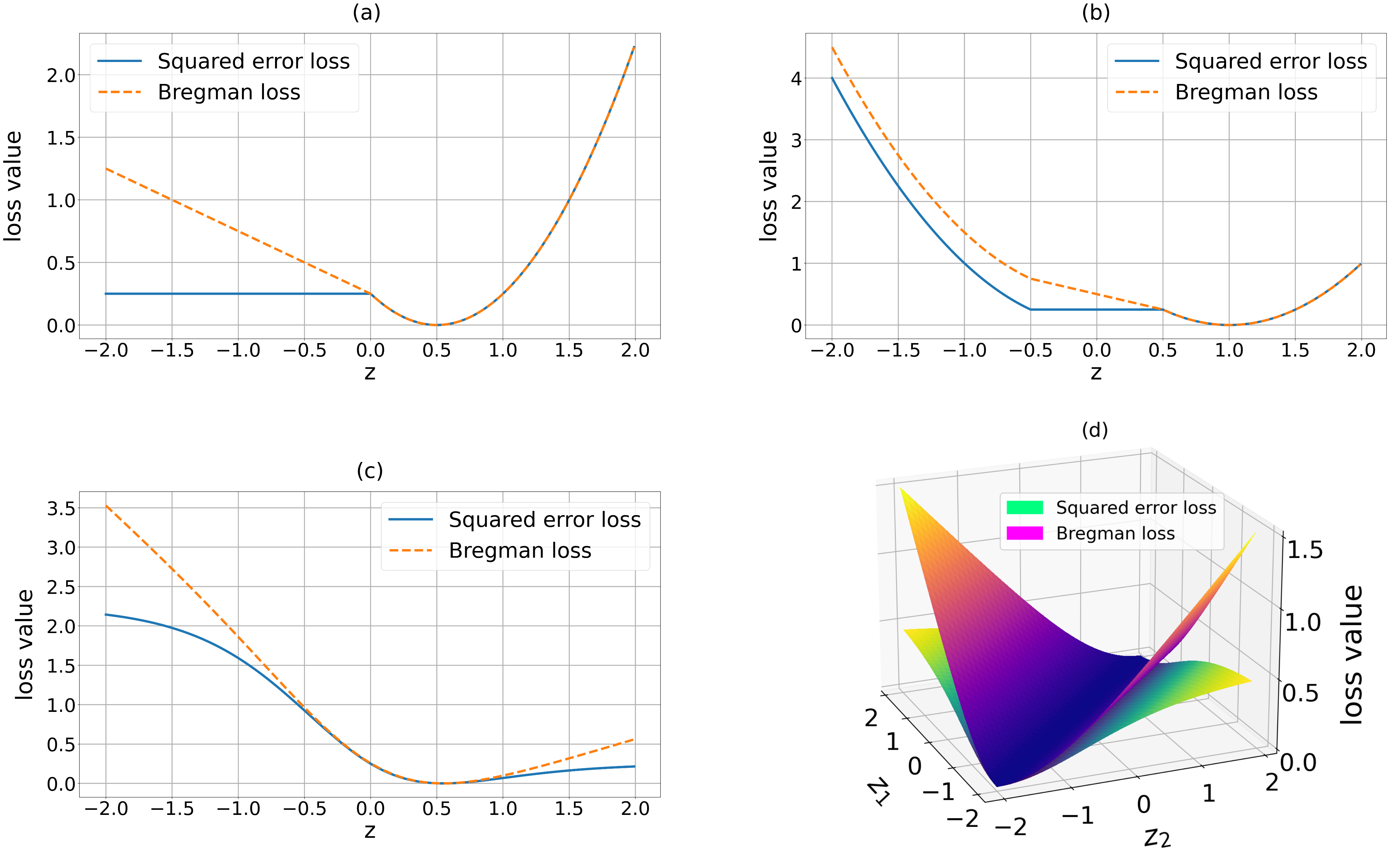
Figure 2: This figure plots the comparison between the Bregman loss function $B_{\Psi}(x,z)$ and the squared Euclidean loss $\frac{1}{2}\|x-\sigma(z)\|^{2}$ for $-2\leq z\leq 2$. We show four cases where each $\sigma$ is: a) the ReLU activation function, b) the soft-thresholding activation function, c) the hyperbolic tangent activation function and (d) the softmax activation function for $n=2$ respectively. The target value $x$ is set to 0.5 when $n=1$ and $x=(0.5,0.5)$ when $n=2$.

3.2 Lifted Bregman training

By replacing the squared Euclidean penalisations in (6) with the Bregman loss function as defined in (12), we have generalised (6) to (13). To demonstrate the advantage of (13), let us consider the case with $s=1$ and one single training sample pair $(x,y)$ again. Using Lemma 8, the gradient of (13) with respect to $\Theta_{l}$ reads

$$\nabla_{\Theta_{l}}B_{\Psi}(x_{l},f(x_{l-1},\Theta_{l}))=(\sigma(f(x_{l-1},\Theta_{l}))-x_{l})J_{f}^{\Theta}(x_{l-1},\Theta_{l})\,,$$

where $J_{f}^{\Theta}$ denotes the Jacobian of $f$ with respect to argument $\Theta$, and for the specific choice $f(x_{l-1},\Theta_{l})=W_{l}^{\top}x_{l-1}+b_{l}$ we observe

$$\sigma(W_{l}^{\top}x_{l-1}^{i}+b_{l})-x_{l}^{i}=0\,,$$

as the optimality condition of (13) w.r.t. the bias term $b_{l}$.

This shows that we guarantee network consistency, i.e. $x_{l}^{i}=\sigma(W_{l}^{\top}x_{l-1}^{i}+b_{l})$, for all layers $l$. In other words, the network is truly nonlinear in contrast to the lifted networks described in Section 2.3.2, and computing the optimality condition with respect to network parameters does not require differentiation of the activation function as in MAC-QP.

In Appendix A.1 we discuss other works related to the lifted Bregman training framework and briefly address similarities and differences.

4 Numerical realisation

In this section we discuss different computational strategies to solve Problem (13) numerically. We divide the discussion into deterministic and stochastic strategies.

4.1 Deterministic approaches

For simplicity of notation, we consider only one pair of samples $(x,y)$ in Problem (13) and without loss of generality we assume that the loss function $\ell$ is also a Bregman loss function. In order to efficiently solve (13) we split the objective in (13) into differentiable and non-differentiable parts as follows:

$$E\left(\mathbf{\Theta},\mathbf{X}\right){}={} \sum_{l=1}^{L}B_{\Psi}(x_{l},f(x_{l-1},\Theta_{l}))$$

$${}={} \underbrace{\sum_{l=1}^{L}\frac{1}{2}\|x_{l}\|^{2}+\Psi(x_{l})}_{=:G(\mathbf{X})}+\underbrace{\sum_{l=1}^{L}\left[\left(\frac{1}{2}\|\cdot\|^{2}+\Psi\right)^{\ast}\left(f\left(x_{l-1},\theta_{l}\right)\right)-\left\langle x_{l},f\left(x_{l-1},\theta_{l}\right)\right\rangle\right]}_{=:H(\mathbf{\Theta},\mathbf{X})}$$

$${}={} G(\mathbf{X})+H(\mathbf{\Theta},\mathbf{X})\,.$$

Here $H$ is a smooth-function in both arguments, while $G$ is potentially non-smooth but with closed-form proximal map.

Remark 11

We want to emphasise that (13) can also be split such that the squared Euclidean norm $\frac{1}{2}\|x_{l}\|^{2}$ of each variable $x_{l}$ is part of $H$, and not of $G$. Both splittings are perfectly reasonable, and we arbitrarily chose the one that includes $\frac{1}{2}\|x_{l}\|^{2}$ in $G$ because computing the proximal map of $G$ with added squared Euclidean norm requires only a trivial modification of the proximal map (cf. (Beck, 2017, Theorem 6.13)).

4.1.1 Proximal gradient descent

A straight-forward approach for the computational minimisation of $E$ is proximal gradient descent (cf. Teboulle (2018)), also known as forward-backward splitting (Lions and Mercier, 1979). This method is a special instance of the following Bregman proximal algorithm (Censor and Zenios, 1992; Teboulle, 1992; Chen and Teboulle, 1993; Eckstein, 1993) that aims at finding minimisers of $E$ via the iteration

$$\left(\begin{matrix}\mathbf{\Theta}^{k+1}\\ \mathbf{X}^{k+1}\end{matrix}\right)=\operatorname*{\arg\min}_{\mathbf{\Theta},\mathbf{X}}\left\{E\left(\mathbf{\Theta},\mathbf{X}\right)+D_{J}\left(\left(\begin{matrix}\mathbf{\Theta}\\ \mathbf{X}\end{matrix}\right),\left(\begin{matrix}\mathbf{\Theta}^{k}\\ \mathbf{X}^{k}\end{matrix}\right)\right)\right\}\,.$$ (16)

Here, $D_{J}$ denotes the Bregman distance with respect to a function $J$, which in case of forward-backward splitting for $E(\mathbf{\Theta},\mathbf{X})=G(\mathbf{X})+H(\mathbf{\Theta},\mathbf{X})$ reads $J(\mathbf{\Theta},\mathbf{X})=\frac{1}{2\tau_{\mathbf{\Theta}}}\sum_{l=1}^{L}\|\Theta_{l}\|^{2}+\frac{1}{2\tau_{\mathbf{X}}}\sum_{l=1}^{L-1}\|x_{l}\|^{2}-H(\mathbf{\Theta},\mathbf{X})$. Here, $\tau_{\mathbf{\Theta}}$ and $\tau_{\mathbf{X}}$ are positive step-size parameters. Then, the optimisation problem $\eqref{eq:bregman-proximal}$ simplifies to

$$\mathbf{\Theta}^{k+1} =\mathbf{\Theta}^{k}-\tau_{\mathbf{\Theta}}\nabla_{\mathbf{\Theta}}H(\mathbf{\Theta}^{k},\mathbf{X}^{k})\,,$$

$$\mathbf{X}^{k+1} =\operatorname*{\arg\min}_{\mathbf{X}}\left\{\frac{1}{2}\left\|\mathbf{X}-\left(\mathbf{X}^{k}-\tau_{\mathbf{X}}\nabla_{\mathbf{X}}H(\mathbf{\Theta}^{k},\mathbf{X}^{k})\right)\right\|^{2}+\tau_{\mathbf{X}}G(\mathbf{X})\right\}\,,$$

$$=\text{prox}_{\tau_{\mathbf{X}}G}\left(\mathbf{X}^{k}-\tau_{\mathbf{X}}\nabla_{\mathbf{X}}H(\mathbf{\Theta}^{k},\mathbf{X}^{k})\right)$$

for initial values $\mathbf{\Theta}^{0}$ and $\mathbf{X}^{0}$. More precisely, the updates with the previous definition of $G$ and $H$ read

$$\Theta_{l}^{k+1}{}={} \Theta_{l}^{k}-\tau_{\mathbf{\Theta}}\left(\text{prox}_{\Psi}\left(f(x_{l-1}^{k},\Theta_{l}^{k})\right)-x_{l}^{k}\right)J_{f}^{\mathbf{\Theta}}(x_{l-1}^{k},\Theta_{l}^{k})\,,$$ (17a)

$$x_{j}^{k+1}{}={} \text{prox}_{\frac{\tau_{\mathbf{X}}}{1+\tau_{\mathbf{X}}}\Psi}\left(\frac{1}{1+\tau_{\mathbf{X}}}\left(x_{j}^{k}-\tau_{\mathbf{X}}\left(\left(\text{prox}_{\Psi}\left(f(x_{j}^{k},\Theta_{j+1}^{k})\right)-x_{j+1}^{k}\right)J_{f}^{x}(x_{j}^{k},\Theta_{j+1}^{k})\right.\right.\right.$$ (17b)

$$\qquad\qquad\qquad\left.\left.\left.-f(x_{j-1}^{k},\Theta_{j}^{k})\vphantom{\frac{1}{1+\tau_{\mathbf{X}}}}\right)\right)\right)\,,$$

for $l\in\{1,\ldots,L\}$ and $j\in\{1,\ldots,L-1\}$, where $J_{f}^{\Theta}$ and $J_{f}^{x}$ denote the Jacobians of $f$ with respect to $\Theta$ and $x$, respectively.

Example 3

Suppose we design a feed-forward network architecture with $\Psi=\chi_{\geq 0}$, which implies $\text{prox}_{\Psi}(z)=\max(z,0)$, and $f(x,\Theta_{l})=W^{\top}_{l}x+b_{l}$, for $\Theta_{l}=(W_{l},b_{l})$. Then (17) reads

$$W_{l}^{k+1} =W_{l}^{k}-\tau_{W}\,x_{l-1}^{k}\left(\max\left((x_{l-1}^{k})^{\top}W_{l}^{k}+(b_{l}^{k})^{\top},0\right)-(x_{l}^{k})^{\top}\right)\,,$$

$$b_{l}^{k+1} =b_{l}^{k}-\tau_{b}\,\left(\max\left((W_{l}^{k})^{\top}x_{l-1}^{k}+b_{l}^{k}\right)-x_{l}^{k},0\right)\,,$$

$$x_{j}^{k+1} =\max\left(\frac{x_{j}^{k}-\tau_{x}\left(W_{j+1}^{k}\max\left((W_{j+1}^{k})^{\top}x_{j}^{k}+b_{j+1}^{k},0\right)-x_{j+1}^{k}\right)-(W_{j}^{k})^{\top}x_{j-1}^{k}-b_{j}^{k}}{1+\tau_{x}},0\right)\,,$$

for $l\in\{1,\ldots,L\}$, $j\in\{1,\ldots,L-1\}$ (with input $x_{0}=x$ and output $x_{L}=y$), $k\in\mathbb{N}$ and the step-size parameters $\tau_{\mathbf{\Theta}}=(\tau_{W},\tau_{b})$ and $\tau_{\mathbf{X}}=\tau_{x}$.

Note that many modifications of proximal gradient descent can be applied, such as proximal gradient descent with Nesterov or Heavy-ball acceleration (Nesterov, 1983; Huang et al., 2013; Teboulle, 2018; Mukkamala et al., 2020). In Appendix B, we also describe how $E$ can be minimised with alternating minimisation approaches such as coordinate descent and the alternating direction method of multipliers that better exploit the structure of the objective for distributed optimisation.

4.1.2 Regularisation of network parameters

In empirical risk minimisation, it is common to design regularisation methods that substitute the empirical risk minimisation process, in order to combat ill-conditioning of the empirical risk minimisation and to improve the validation error. In the context of risk minimisation, regularisations are approximate inverses of the model function w.r.t. the model parameters. For more information about regularisation, we refer the interested reader to Engl et al. (1996); Benning and Burger (2018) for an overview of deterministic regularisation, to Stuart (2010) for a Bayesian perspective on regularisation and De Vito et al. (2005, 2021) for regularisation in the context of machine learning. We discuss the two common approaches of variational and iterative regularisation and how to incorporate them into the lifted Bregman framework.

Variational regularisation. In variational regularisation, a positive multiple of a regularisation function is added to the empirical risk formulation. Denoting this regularisation function by $R$, we can simply modify $E$ to

$$E(\mathbf{\Theta},\mathbf{X})=\sum_{l=1}^{L}B_{\Psi}\left(x_{l},f(x_{l-1},\Theta_{l})\right)+R(\mathbf{\Theta})\,.$$

However, there is a catch with this modification that is probably not obvious at first glance. Suppose $R$ is differentiable for now. If we compute the optimality condition w.r.t. a particular $\Theta_{l}$, we observe

$$0 =\nabla_{\Theta_{l}}\left(B_{\Psi}(x_{l}^{\ast},f(x_{l-1}^{\ast},\Theta_{l}^{\ast}))+R(\Theta_{1}^{\ast},\ldots,\Theta_{l}^{\ast},\ldots,\Theta^{\ast}_{L})\right)\,,$$

$$=\left(\sigma(f(x_{l-1}^{\ast},\Theta_{l}^{\ast}))-x_{l}^{\ast}\right)J_{f}^{\Theta}(x_{l-1}^{\ast},\Theta_{l}^{\ast})+\nabla_{\Theta_{l}}R(\mathbf{\Theta}^{\ast})\,.$$

Without $\nabla_{\Theta_{l}}R(\mathbf{\Theta}^{\ast})$, the condition $0=\left(\sigma(f(x_{l-1}^{\ast},\Theta_{l}^{\ast}))-x_{l}^{\ast}\right)J_{f}^{\Theta}(x_{l-1}^{\ast},\Theta_{l}^{\ast})$ guarantees network consistency $\sigma(f(x_{l-1}^{\ast},\Theta_{l}^{\ast}))=x_{l}^{\ast}$ up to an element in the nullspace of $J_{f}^{\Theta}(x_{l-1}^{\ast},\Theta_{l}^{\ast})$. Unless $\nabla_{\Theta_{l}}R(\mathbf{\Theta}^{\ast})=0$, this network consistency will be violated when adding a regularisation term $R$ that acts on the network parameters. Because of this shortcoming, we consider iterative regularisation strategies as an alternative in the next subsection.

Iterative regularisation. When we iteratively update the parameters $\mathbf{\Theta}$ and $\mathbf{X}$ via approaches like (16) or (38), we can convert them into iterative regularisations known as (linearised) Bregman iterations (Osher et al., 2005; Cai et al., 2009; Benning and Burger, 2018). We achieve this simply by including a regularisation function in the Bregman function. For example, in (16) we can choose $J(\mathbf{\Theta},\mathbf{X})=\frac{1}{\tau_{\mathbf{\Theta}}}\left(R(\mathbf{\Theta})+\frac{1}{2}\sum_{l=1}^{L}\|\Theta_{l}\|^{2}\right)+\frac{1}{2\tau_{\mathbf{X}}}\sum_{l=1}^{L-1}\|x_{l}\|^{2}-H(\mathbf{\Theta},\mathbf{X})$ instead of $J(\mathbf{\Theta},\mathbf{X})=\frac{1}{2\tau_{\mathbf{\Theta}}}\sum_{l=1}^{L}\|\Theta_{l}\|^{2}+\frac{1}{2\tau_{\mathbf{X}}}\sum_{l=1}^{L-1}\|x_{l}\|^{2}-H(\mathbf{\Theta},\mathbf{X})$. Note that the choice of $J$ doesn’t affect the optimality conditions of $E$, but it allows to control the regularity of the model parameters $\mathbf{\Theta}$. If the objective $E$ has multiple or even infinitely many minimisers, a different choice of $R$ enables convergence towards network parameters with desired properties such as sparsity of the parameters.

In the context of neural networks, such a strategy has first been applied in Benning et al. (2021) to train neural networks and also control the rank of the network parameters. We can achieve the same by choosing $R$ to be a positive multiple of the nuclear norm. Recently, in Bungert et al. (2021), the idea of (linearised) Bregman iterations has been extended to stochastic first-order optimisation in order to effectively train neural networks with sparse parameters. Networks with sparse network parameters can be obtained by setting $R$ to a positive multiple of the one-norm.

4.1.3 Regularisation of auxiliary variables

One of the great advantages of a lifted network approach is that it is straight-forward to also impose regularisation on the auxiliary variables $\{x_{l}\}_{l=1}^{L-1}$. This can be extremely useful in different contexts. Suppose, for example, that we want to train an autoencoder neural network with sparse encoding. This would require us to impose regularity on the output of the encoder network, which is equal to one of the auxiliary variables in the lifted network formulation. We will discuss such a sparse autoencoder approach in greater detail in Section 5.2. In the following, we want to discuss how to adapt the two regularisation strategies discussed in the previous section.

Variational regularisation. In contrast to variational regularisation of network parameters, adding a regularisation function $R$ that acts on $\mathbf{X}$ to the objective $E$ does not impact the optimality system of $E$ w.r.t. the network parameters $\mathbf{\Theta}$. Hence, network consistency will not be violated and regularity can be imposed this way.

Iterative regularisation. In identical fashion to the previous section, we can incorporate regularity by modifying Bregman functions, for example in (16) via $J(\mathbf{\Theta},\mathbf{X})=\frac{1}{2\tau_{\mathbf{\Theta}}}\sum_{l=1}^{L}\|\Theta_{l}\|^{2}+\frac{1}{\tau_{\mathbf{X}}}\left(R(\mathbf{X})+\frac{1}{2}\sum_{l=1}^{L-1}\|x_{l}\|^{2}\right)-H(\mathbf{\Theta},\mathbf{X})$ instead of $J(\mathbf{\Theta},\mathbf{X})=\frac{1}{2\tau_{\mathbf{\Theta}}}\sum_{l=1}^{L}\|\Theta_{l}\|^{2}+\frac{1}{2\tau_{\mathbf{X}}}\sum_{l=1}^{L-1}\|x_{l}\|^{2}-H(\mathbf{\Theta},\mathbf{X})$.

4.2 Stochastic approaches

Having discussed suitable deterministic approaches for the minimisation of $E$, we want to describe how to adopt such approaches in stochastic settings. In particular, we consider the objective $E$ from the previous section, but for $s$ pairs of samples $\{(x_{i},y_{i})\}_{i=1}^{s}$:

$$E(\mathbf{\Theta},\mathbf{X})=\frac{1}{s}\sum_{i=1}^{s}\sum_{l=1}^{L}B_{\Psi}\left(x_{l}^{i},f(x_{l-1}^{i},\Theta_{l})\right)\,.$$ (18)

Here, $\mathbf{\Theta}=\{\Theta_{l}\}_{l=1}^{L}$ is again the short-hand notation for all parameters (for all layers), but $\mathbf{X}=\{x_{l}^{i}\}_{l=1,\ldots,L}^{i=1,\ldots,s}$ is the collection of auxiliary variables that now also depend on the input and output samples $\{(x_{i},y_{i})\}_{i=1}^{s}$. We want to investigate which stochastic minimisation methods we can formulate that only use a (random) subset of the indices at every iteration.

The most straight-forward approach is to use out-of-the-box, state-of-the-art first order methods like stochastic gradient descent (Robbins and Monro, 1951; Kiefer and Wolfowitz, 1952) or variants of it. Since the function $E$ is additively composed of a smooth ($H$) and a non-smooth ($G$) function, the overall function $E$ is non-smooth. Hence, gradient-based first-order methods applied directly to $E$ become subgradient-based first-order methods, with potentially slower convergence and artificial critical points, even though these usually do not pose serious issues with high probability (cf. Bolte and Pauwels (2020)). However, fully explicit optimisation methods whose convergence speed depends on Lipschitz constants of gradients can easily suffer from an explosion of these constants when applied directly to non-smooth functions.

Another disadvantage of applying methods such as stochastic gradient descent and evaluating the gradient or subgradient via backpropagation is that it is not straight-forward to easily distribute the computation of parameters as it is the case for distributed optimisation approaches such as the ones described in Section 2.3, respectively (Carreira-Perpinan and Wang, 2014; Askari et al., 2018; Gu et al., 2020).

And not to forget, we lose the advantage that the differential of the Bregman loss function $B_{\Psi}$ does not require the differentiation of the activation function if we try to differentiate the non-smooth part $G$. We therefore discuss three alternative optimisation strategies; we begin with a discussion of stochastic proximal gradient descent, then we continue to focus on data-parallel (implicit) optimisation, before we conclude with implicit stochastic gradient descent.

4.2.1 Stochastic proximal gradient descent

Given the structure of $E$, it seems natural to consider stochastic proximal gradient descent (Duchi and Singer, 2009; Rosasco et al., 2019). However, most approaches, such as the ones discussed in Rosasco et al. (2019), assume a structure of the form

$$E(\mathbf{\Theta})=G(\mathbf{\Theta})+\frac{1}{s}\sum_{i=1}^{s}H_{i}(\mathbf{\Theta})\,,$$

where every $H_{i}$ is differentiable and $G$ is proximable. In comparison, our setting is of the form

$$E(\mathbf{\Theta},\mathbf{X})=\frac{1}{s}\sum_{i=1}^{s}\left(G(\mathbf{X}_{i})+H(\mathbf{\Theta},\mathbf{X}_{i})\right)\,,$$ (19)

where $\mathbf{X}_{i}$ is the collection $\{x_{1}^{i},\ldots,x_{L-1}^{i}\}$ for each index $i\in\{1,\ldots,s\}$. Here, the function $G$ only depends on the samples $\mathbf{X}$ and optimising with respect to $\mathbf{X}$ remains deterministic, while we can optimise $\mathbf{\Theta}$ by only using (random) subsets of $\{1,\ldots,s\}$ at each iteration. A possible approach is to compute

$$\mathbf{\Theta}^{k+1} =\mathbf{\Theta}^{k}-\tau_{\mathbf{\Theta}}^{k}\nabla_{\mathbf{\Theta}}H(\mathbf{\Theta}^{k},\mathbf{X}_{i}^{k})\,,$$

$$\mathbf{X}_{i}^{k+1} =\text{prox}_{\tau_{\mathbf{X}_{i}}G}\left(\mathbf{X}_{i}^{k}-\tau_{\mathbf{X}_{i}}\nabla_{\mathbf{X}_{i}}H(\mathbf{\Theta}^{k},\mathbf{X}_{i}^{k})\right)\,,$$

or alternating variants. It should be straight-forward to show convergence for such an algorithm with standard arguments in the simpler but unrealistic setting in which both $H$ and $G$ are jointly-convex in both $\mathbf{X}$ and $\mathbf{\Theta}$. However, proving such a result is beyond the scope of this work.

4.2.2 Data-parallel optimisation

Instead of minimising (19) for all samples at once, one can split the indices into $m$ randomised batches $B_{p}$ with $\bigcup_{p=1}^{m}B_{p}=\{1,\ldots,s\}$ and $\bigcap_{p=1}^{m}B_{p}=\emptyset$. We can then solve the optimisation problems for each batch individually and subsequently average all results, which is also widely known as model averaging (Zinkevich et al., 2010; McDonald et al., 2010). The optimisation problem for each batch can be solved in parallel with any of the methods described in Section 4.1. In the next section, we focus on an alternative implicit optimisation technique that can be performed sequentially for all batches or in parallel, which in its sequential form is known as implicit stochastic gradient descent.

4.2.3 Implicit stochastic gradient descent

Implicit stochastic gradient descent (Toulis and Airoldi, 2017) is a straight-forward modification of stochastic gradient descent where each update is implicit. Note that mini-batch stochastic gradient descent for an objective $E(\mathbf{\Theta})=\frac{1}{s}\sum_{i=1}^{s}f_{i}(\mathbf{\Theta})$, which in its usual form reads

$$\mathbf{\Theta}^{k+1}=\mathbf{\Theta}^{k}-\frac{\tau^{k}}{|B_{p}|}\sum_{i\in B_{p}}\nabla f_{i}(\mathbf{\Theta}^{k})\,,$$ (20)

can be formulated as

$$\mathbf{\Theta}^{k+1}=\operatorname*{\arg\min}_{\mathbf{\Theta}}\left\{\frac{1}{|B_{p}|}\sum_{i\in B_{p}}f_{i}(\mathbf{\Theta})+D_{J_{k}}(\mathbf{\Theta},\mathbf{\Theta}^{k})\right\}\,,$$ (21)

see for instance Benning and Riis (2021), which shows that it is also a special-case of stochastic mirror descent (Nemirovski et al., 2009), and where $J_{k}=\frac{1}{2\tau^{k}}\|\mathbf{\Theta}\|^{2}-\frac{1}{|B_{p}|}\sum_{i\in B_{p}}f_{i}(\mathbf{\Theta})$, with $D_{J_{k}}$ being the corresponding Bregman distance. Here, the choice of function $J_{k}$ ensures the explicitness of mini-batch stochastic gradient descent (cf. (Benning and Riis, 2021, Equation (6))). We can obviously replace $J_{k}$ simply with $\frac{1}{2\tau^{k}}\|\mathbf{\Theta}\|^{2}$, so that (21) changes to

$$\mathbf{\Theta}^{k+1}=\operatorname*{\arg\min}_{\mathbf{\Theta}}\left\{\frac{1}{|B_{p}|}\sum_{i\in B_{p}}f_{i}(\mathbf{\Theta})+\frac{1}{2\tau^{k}}\|\mathbf{\Theta}-\mathbf{\Theta}^{k}\|^{2}\right\}\,.$$ (22)

This method, proposed and studied in Toulis and Airoldi (2017) is similar to classical stochastic gradient descent, but the update can no longer be computed explicitly and requires the implicit solution of a deterministic optimisation problem at each iteration. If we want to connect this to Section 4.2.2, we can modify (22) to not use the previous argument $\mathbf{\Theta}$ as the second argument in the Bregman distance, but to use the average of the previous epoch, i.e.

$$\mathbf{\Theta}^{k+1}_{p}=\operatorname*{\arg\min}_{\mathbf{\Theta}}\left\{\frac{1}{|B_{p}|}\sum_{i\in B_{p}}f_{i}(\mathbf{\Theta})+\frac{1}{2\tau^{k}_{p}}\left\|\mathbf{\Theta}-\frac{1}{m}\sum_{q=1}^{m}\mathbf{\Theta}^{k}_{q}\right\|^{2}\right\}\,,$$ (23)

for $p\in\{1,\ldots,m\}$. The advantage of (23) over (22) is that each batch can be processed in parallel, at the cost of potentially inferior convergence speed. Applying (22) to objective (18) yields the iteration

$$(\mathbf{\Theta}^{k+1},\mathbf{X}^{k+1})=\operatorname*{\arg\min}_{\mathbf{\Theta},\mathbf{X}}\left\{\frac{1}{|B_{p}|}\sum_{i\in B_{p}}\sum_{l=1}^{L}B_{\Psi}(x_{l}^{i},f(x_{l-1}^{i},\Theta_{l})))+\frac{1}{2\tau^{k}}\|\mathbf{\Theta}-\mathbf{\Theta}^{k}\|^{2}\right\}\,.$$ (24)

It is important to point out that in (24) not all $x$-variables are updated at once, but only the variables for the current batch $B_{p}$. Hence, an entire epoch is required to update all $x$-variables once. For simplicity, we introduce a short-hand notation $X_{l}^{p}=\{x_{l}^{i}\}^{i\in B_{p}}$ to denote the collection of $x_{l}$-variables associated with the current batch $B_{p}$.

As an example, consider the problem of training a feed-forward network by minimising (13) with additional variational regularisation acting on the auxiliary variable as described in Section 4.1.3, for $f(x_{l-1},\Theta_{l})=W^{\top}_{l}x_{l-1}+b_{l}$. Using (24) and (17) for each individual minimisation problem per mini-batch, the overall algorithm is summarised in Algorithm 1. Here, $K$ refers to the number of epochs, and $N$ refers to the number of iterations of the inner algorithm.

Algorithm 1 Implicit Stochastic Lifted Bregman Learning

  Initialise $\Theta_{l}^{0}$ for each $l\in\{1,2,\ldots,L\}$  

  for $k\in\{1,2,\ldots,K\}$ do

     Choose $B_{p}\subset\{1,2,\dots s\}$ either at random or deterministically.

     Initialise $x^{i}_{j}=\sigma_{j}(f(x_{j-1}^{i},\Theta_{j}^{k}))\text{ for each }i\in B_{p}\text{ and }j\in\{1,2,\ldots,L-1\}.$

     for $l\in\{L,\ldots 1\}$ and $j\in\{L-1,\ldots 1\}$  do

        for $n\in\{0,1,\ldots,N-1\}$ do

           Compute step size parameters $\tau_{\Theta}$ and $\tau_{x}$.

           $\displaystyle\begin{aligned} \Theta_{l}^{n+1}\leftarrow\Theta_{l}^{n}-\tau_{\Theta}\left(\frac{1}{|B_{p}|}\sum_{i\in B_{p}}\left(\text{prox}_{\Psi}\right.\right.&\left.\left(f(x_{j-1}^{i,n},\Theta_{l}^{n})\right)-x_{j}^{i,n}J_{f}^{\Theta}(x_{j-1}^{i,n},\Theta_{l}^{n})\right)\\ &\left.\phantom{\sum_{i\in B_{p}}}+\tau^{k}(\Theta_{l}^{n}-\Theta_{l}^{k-1})\right)\,\end{aligned}$

           for $i\in B_{p}$ do

              

$$x_{j}^{i,n+1}\leftarrow \text{prox}_{\frac{\tau_{x}}{|B_{p}|+\tau_{x}}\left(\Psi+R\right)}\left(\frac{|B_{p}|}{|B_{p}|+\tau_{x}}\left(x_{j}^{i,n}+\frac{\tau_{x}}{|B_{p}|}\left(f(x_{n-1}^{i,n},\Theta_{j}^{k})\right.\right.\right.$$

$$\qquad\left.\left.\left.-\left(\text{prox}_{\Psi}\left(f(x_{j}^{i,n},\Theta_{j+1}^{n})\right)-x_{j+1}^{i,n}\right)J_{f}^{x}(x_{j}^{i,n},\Theta_{j+1}^{n})\right)\right)\right)\,$$

           end for

        end for

        $\Theta_{l}^{k}\leftarrow\Theta_{l}^{N}$

     end for

  end for

Note that similar to the examples described in Section 4.1, one can replace the squared-two-norm term in (24) with a Bregman distance term to design explicit-implicit variants of (24). For example, if we replace $\frac{1}{2\tau^{k}}\|\mathbf{\Theta}-\mathbf{\Theta}\|^{2}$ with the Bregman distance $D_{J_{k}}(\mathbf{\Theta},\mathbf{\Theta}^{k})$ for the choice $J_{k}(\mathbf{\Theta})=\frac{1}{\tau^{k}}\|\mathbf{\Theta}\|^{2}-\frac{1}{|B_{p}|}\sum_{i\in B_{p}}\sum_{l=1}^{L}B_{\Psi}(x_{l}^{i},f(x_{l-1}^{i},\Theta_{l})))$, we can make (24) explicit with respect to the parameters $\mathbf{\Theta}$, with the potential drawback of more complicated implicit optimisation problems for $\mathbf{X}$.

5 Example problems

In this section, we present some example problems and demonstrate how the lifted Bregman approach can be utilised to train neural networks. We discuss both supervised and unsupervised learning examples. We consider the supervised learning task of image classification, and the unsupervised learning task of training a sparse autoencoder and a sparse denosing autoencoder.

5.1 Classification

The first example problem that we consider is image classification. In the fully supervised learning setting, pairwise data samples $\{x_{i},y_{i}\}_{i=1}^{s}$ are provided, with each $x_{i}$ being an input image while $y_{i}$ represents the corresponding class label. The task is to train a classifier that correctly categorises images by assigning the correct labels. Training an $L$-layer network via the lifted Bregman approach can be formulated as the following minimisation problem:

$$\min_{\mathbf{\Theta},\mathbf{X}}\frac{1}{s}\sum_{i=1}^{s}\left[B_{\Psi_{L}}\left(y^{i},x_{L}^{i}\right)+\sum_{l=1}^{L-1}\,B_{\Psi_{l}}\left(x_{l}^{i},f(x_{l-1}^{i},\Theta_{l})\right)\right]\,.$$ (25)

Note that we allow for different functions $\Psi_{l}$ in order to allow for different activation functions for different layers. The loss function $\ell$ in the Learning Problem (2) can also be chosen to be a Bregman loss function $B_{\Psi_{L}}\left(y^{i},x_{L}^{i}\right)$, which here measures the discrepancy between the predicted output and the target labels. Note that the special case for $L=1$ has already been covered in Wang and Benning (2020).

5.2 Sparse autoencoder

For the next two application examples we consider sparse autoencoders. Sparse autoencoders aim at transforming signals into sparse latent representations, effectively compressing the original signals. In this section, we formulate an unsupervised, regularised empirical risk minimisation for sparse autoencoders in the spirit of Section 4.1.3.

An autoencoder is a composition of two mathematical operators: an encoder and a decoder. The encoder maps input data onto latent variables in the latent space. The latent variables are usually referred to as code. The decoder aims to recover the input data from the code. Unlike regular autoencoders that reduce the dimension of the latent space, the latent space of a sparse autoencoder can have the same or an even larger dimension than the input space. The compression of the input data is achieved by ensuring that only relatively few coefficients of the code are non-zero. The advantage over conventional autoencoders is that the position of the non-zero coefficients can vary for individual signals.

Sparsity on latent nodes can be achieved by explicitly regularising the latent representations (Ng et al., 2011; Xie et al., 2012). One approach is to penalise the Kullback Leibler divergence between the hidden node sparsity rate and the target sparsity level during training (Ng et al., 2011; Xie et al., 2012). In this work, we explore an alternative approach using $\ell_{1}$ regularisation to promote sparsity of the codes in the spirit of compressed sensing (cf. Candès et al. (2006); Donoho (2006)), and proceed as discussed in Section 4.1.3. We formulate the sparse autoencoder training problem as the minimisation of the energy

$$\min_{\mathbf{\Theta},\mathbf{X}}\frac{1}{s}\sum_{i=1}^{s}\left[B_{\Psi_{L}}\left(x_{0}^{i},x_{L}^{i}\right)+\sum_{l=1}^{L-1}\lambda_{l}\,B_{\Psi_{l}}\left(x_{l}^{i},f(x_{l-1}^{i},\Theta_{l})\right)+\alpha\|x_{L/2}^{i}\|_{1}\right]\,,$$ (26)

with $\{x_{0}^{i}\}_{i=1}^{s}$ denoting the provided, unlabelled data. Here $\{x_{L/2}^{i}\}_{i=1}^{s}$ are the activation variables that correspond to the code, i.e. the output of the encoder, which we arbitrarily chose at the middle layer $\frac{L}{2}$. The regularisation parameter $\alpha\geq 0$ is the hyper-parameter controlling the sparsity of the codes.

As discussed in Section 4.1.3, one of the advantages of the lifted Bregman framework is that additional regularisation terms acting on the activation variables can easily be incorporated into various algorithmic frameworks.

5.3 Sparse denoising autoencoder

We present the third example that aims at learning sparse autoencoders for denoising. During training, a denoising autoencoder receives corrupted versions $\tilde{x}$ of the input $x$ and aims to reconstruct the clean signal $x$. By changing the reconstruction objective, the denoising autoencoder is compelled to learn a robust mapping against small random perturbations and must go beyond finding an approximation of the identity function (Bengio et al., 2013; Alain and Bengio, 2014). In analogy to (26), the proposed learning problem reads

$$\min_{\mathbf{\Theta},\mathbf{X}}\frac{1}{s}\sum_{i=1}^{s}\left[B_{\Psi_{L}}\left(x_{0}^{i},\tilde{x}_{L}^{i}\right)+\sum_{l=1}^{L-1}\lambda_{l}\,B_{\Psi_{l}}\left(\tilde{x}_{l}^{i},f(\tilde{x}_{l-1}^{i},\Theta_{l})\right)+\alpha\|\tilde{x}_{L/2}^{i}\|_{1}\right]\,,$$ (27)

where $\tilde{x}_{0}^{i}$ and $x_{0}^{i}$ are the corrupted and clear input data respectively. Similar to training sparse autoencoders, we regularise the $\ell_{1}$-norm of the hidden code, i.e. the middle layer activation variable $x_{L/2}$ to enforce activation sparsity.

6 Numerical results

In this section, we present numerical results for the example applications described in Section 5. We implement the lifted Bregman framework with Algorithm 1 and compare this method to three first-order methods: 1) the classical (sub-)gradient descent method described in (3), 2) the stochastic (sub-)gradient descent method which follows (20), and 3) the implicit stochastic (sub-)gradient descent that follows (22).

All results have been computed using PyTorch 3.7 on an Intel Xeon CPU E5-2630 v4. Code related to this publication will be made available through the University of Cambridge data repository at https://doi.org/10.17863/CAM.86729.

We use the MNIST dataset (LeCun et al., 1998) and the Fashion-MNIST dataset (Xiao et al., 2017) for all numerical experiments. For both datasets, we pre-process the data by centring the images and by converting the labels to one-hot vector encodings.

6.1 Classification

For the classification task, we follow the work of Zach and Estellers (2019) and consider a fully connected network with $L=4$ layers with ReLU activation functions. More specifically, we use $f(x_{l-1},\Theta_{l})=W_{l}^{\top}x_{l-1}+b_{l}$ with $W_{l}\in\mathbb{R}^{m_{l-1}\times m_{l}}$ and $b_{l}\in\mathbb{R}^{m_{l}\times 1}$ where $m_{1}=784$, $m_{2}=m_{3}=64$ and $m_{4}=10$. In solving the classification problem described in Section 5.1, we do not include any additional regularisation term and set $R\equiv 0$ in the learning objective (25). We use the Mean Squared Error (MSE) between the prediction and the one-hot encoded target values as our classification loss, which also is a Bregman loss function (12) for $\Psi_{L}\equiv 0$.

We apply Algorithm 1 to train the classification network with the lifted Bregman framework. In solving each mini-batch sub-problem (24), we run a maximum of $N=15$ iterations with $\tau^{k}=100$. The other step-size parameters are set to $\tau_{W_{l}}=1.99/\left(\|X_{l}^{p}\|_{2}^{2}+\tau_{k}/2\right)$ and $\tau_{x}=1.99/\|W_{l}\|_{2}^{2}$ to ensure convexity of $J$ in (16). For comparison, the same network architecture is trained via the stochastic (sub-)gradient method (20) in combination with the back-propagation Algorithm 2, which we will refer to as the SGD-BP approach. Out of the learning rates $\{1\times 10^{-5},5\times 10^{-5},1\times 10^{-4},5\times 10^{-4},1\times 10^{-3},5\times 10^{-3},1\times 10^{-2},5\times 10^{-2},1\times 10^{-1},5\times 10^{-1}\}$, we found that $1\times 10^{-3}$ works best empirically in terms of receiving lowest training objective values.

For both the MNIST and Fashion-MNIST datasets, we use 60,000 images for training and 10,000 images for validation. Network parameters in all experiments are identically initialised following Glorot and Bengio (2010). We choose batch size $|B_{k}|=100$ and train the network for 100 epochs.

Table 1 summarises the achieved training and validation classification accuracy after training. For the classical lifted training approach, we quote results from Zach and Estellers (2019). The lifted Bregman scheme achieves comparable classification accuracy to the SGD-BP approach and shows substantial improvements over the classical lifted approach that produces affine-linear networks.

	MNIST		Fashion-MNIST
Model	Train	Test	Train	Test
Standard Lifted Network	85.6%	86.3%	81.4%	80.0%
Lifted Bregman Network	99.3%	96.8%	93.5%	85.7%
SGD-BP	99.6%	96.9%	95.8%	87.9%

Table 1: This table summarises training and test classification accuracies for the MNIST and Fashion-MNIST datasets, where the network is trained with the lifted Bregman approach, the classical lifted training approach and the stochastic (sub-)gradient method with back-propagation.

In Table 2 we present the evaluated percentage of linear activations of the network under different training strategies. This rate computes the percentage of number of nodes in each hidden layer that perform linearly, i.e. ($z^{i}=\max(z^{i},0)$). As described in Section 2.3.2, classical lifted network training produces affine-linear networks. We empirically verify that the lifted Bregman framework overcomes this limitation.

	MNIST			Fashion-MNIST
Model	Layer 1	Layer 2	Layer 3	Layer 1	Layer 2	Layer 3
Standard Lifted Network	99.9%	99.9%	99.9%	99.9%	99.9%	99.9%
Lifted Bregman Network	47.4%	82.2%	70.1%	59.2%	85.7%	64.7%
SGD-BP	40.1%	29.7%	73.6%	32.2%	28.1%	78.4%

Table 2: In this table, we show the percentage of nodes in the network’s hidden layers that act linearly. The network is trained with the lifted Bregman approach, the classical lifted approach and the the stochastic (sub-)gradient method with back-propagation respectively, on both the MNIST and Fashion-MNIST datasets.

6.2 Sparse Autoencoder

As discussed in Section 5.2, we train a fully-connected autoencoder with $L=4$ layers with $f(x_{l-1},\Theta_{l})=W_{l}^{\top}x_{l-1}+b_{l}$. The hidden dimension is set to $m_{l}=784$ for $l=1,\ldots,4$, i.e. there is no explicit reduction in dimension. We use the MSE reconstruction loss and the regularisation parameter $\alpha$ is chosen at $\alpha=0.09$ and does not ensure optimal validation errors, but a sparsity rate of the code of approximately 90% to guarantee an implicit reduction in dimension instead.

Note that the additional regularity on the code can easily be implemented in the lifted Bregman framework provided we choose a suitable activation function for the activation variable that corresponds to the code. Specifically, when the activation variable $x_{2}$ is activated by the soft-thresholding function, the additional non-smooth $\ell_{1}$-norm regularisation term in (26) can easily be incorporated by modifying the $\Psi_{2}$ function in the update step of the $x_{2}$ variable in Algorithm 1. In this example, we apply the soft-thresholding activation function after the second affine-linear transformation and adopt ReLU activation functions for all other layers.

MNIST-1K For this application example, we consider a slightly more challenging learning scenario (referred to as MNIST-1K). We limit the amount of training data, and compare how well the trained network generalises on a larger validation set. We choose $s=1,000$ images from the MNIST dataset at random and use it as our training dataset and use all $10,000$ images from the validation dataset for validation.

We experiment with both deterministic and stochastic implementations of the lifted Bregman framework. For the stochastic implementation (referred to as LBN-S), network parameters are trained via Algorithm 1. We choose batch size $|B_{k}|=20$ and step-size $\tau_{k}=1$. In each batch sub-problem, the minimisation problems are iterated for $N=15$ iterations, with step-sizes computed via $\tau_{w_{l}}=1.99s/(\|X^{p}_{l}\|_{2}^{2}+\tau_{k}/2)$ and $\tau_{b}=1.99$. The deterministic implementation (LBN-D) follows the same update steps described in Algorithm 1 with $\tau^{k}=0$ and $|B_{k}|=s$, i.e. we use all data at every epoch. The step size $\tau_{w_{l}}$ is computed as $1.99s/\|X_{l}\|_{2}^{2}$.

For comparison, we train the autoencoder also with two first-order methods: (sub-)gradient descent (GD-BP), which follows (3), and the stochastic (sub-)gradient descent approach (SGD-BP) described in (20), both in combination with the back-propagation Algorithm (2) for the computation of (sub-)gradients.

As learning objective we choose the MSE loss plus $\alpha$ times the $\ell_{1}$-norm regularisation. Various learning rates in the range $[10^{-4},10^{-1}]$ have been tested. In terms of minimising the training objective values, we find that $4\times 10^{-2}$ and $3\times 10^{-2}$ work optimal for GD-BP and SGD-BP approaches, respectively.

We train the autoencoder network for 100 epochs and plot the decay of the objective values over all epochs in Figure 3 (Left). While the training objective value tracks the sum of reconstruction loss and $\alpha$ times $\ell_{1}$-norm regularisation, the validation objective only records the MSE loss. The sparsity rate per epoch is computed as the percentage of zero-valued entries of the code $X_{2}$, which we visualise in Figure 3 (Right).

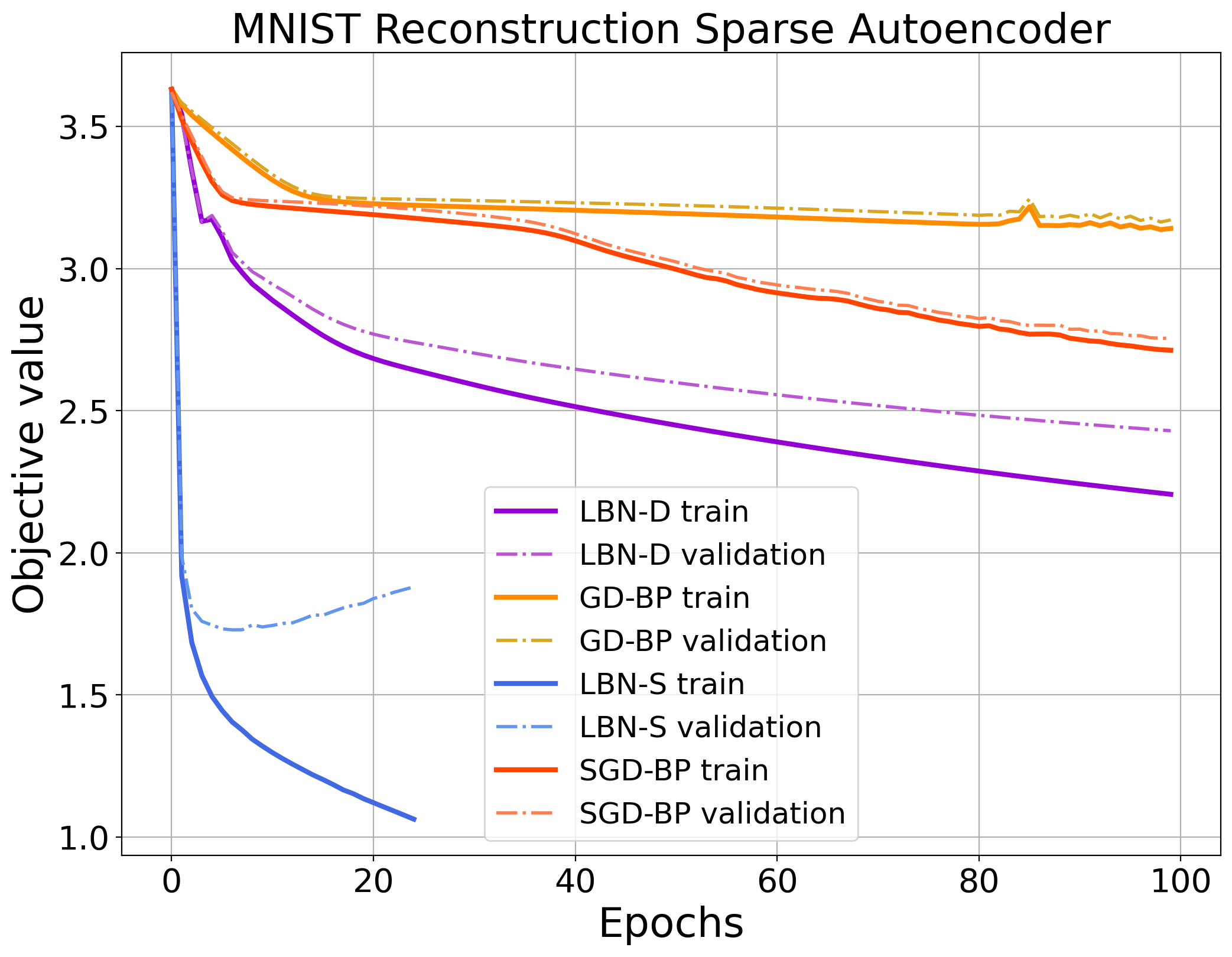
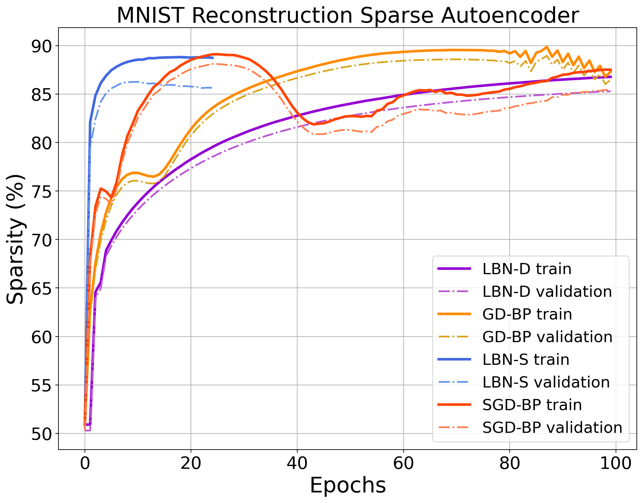
Figure 3: Sparse Autoencoder trained on MNIST-1K dataset. Left: Objective values per epoch for each learning scheme as explained in Section 6.2. The training objectives (solid lines) record MSE loss plus $\ell_{1}$-norm regularisation and the validation objectives (dashed lines) report the MSE loss values. Right: Sparsity level of the code per training epoch for each learning scheme.

Overall, the lifted Bregman implementations outperform the (sub-)gradient-based first-order methods, although it should be emphasised that LBN-D and LBN-S are computationally more expensive than GD-BP and SGD-BP (and we will present a fairer comparison in the denoising autoencoder section). We also observe that the stochastic variants of both learning schemes can speed up training and provide faster convergence compared to their deterministic counterparts. The effect on LBN-D is more noticeable than on GD-BP as we observe significant drops in objective value in early training epochs.

The validation loss curves recovered with GD-BP and SGD-BP follow their training curves quite closely. LBN-S on the other hand shows a drop of the validation loss before it increases again after around 7 epochs. A similar increase could be observed for LBN-D if we were to train the parameters for more epochs. This demonstrates that we can overfit this autoencoder with 3136 parameters to the 1000 training data samples of dimension 784 with the LBN algorithms, but we do not observe the same phenomenon with the GD-BP and SGD-BP algorithms. In light of Zhang et al. (2021), this raises the question whether good generalisation properties of neural networks are more down to the choice of optimisation technique than architectural design choices.

When looking at a sparsity rate comparison per epoch, we notice the oscillatory behaviours of both (sub-)gradient based methods. As their sparsity levels climb higher, their corresponding objective value curves remain stagnant. The decreases in objective values for both GD-BP and SGD-BP roughly coincide with when their sparsity rate drops. In contrast, we can see that the lifted Bregman implementations handle the same level of regularisation more smoothly. They achieve similar sparsity levels in the end but in a more stable and controlled manner.

In Figure 5, we visualise ground truth images and reconstructions of two randomly selected images from the training dataset for all four training approaches. In Figure 5 we visualise the same quantities but based on two randomly selected images from the validation dataset. All four approaches are capable of providing good quality reconstructions in light of the high sparsity levels, for both the training and testing datasets. However, the proposed LBN-D and LBN-S approaches provide sharper edges and finer details than the GD-BP and SGD-BP approaches. LBN-S slightly outperforms LBN-D and is capable of defining even clearer and sharper edges. More reconstructed images can be found in Appendix C.1.

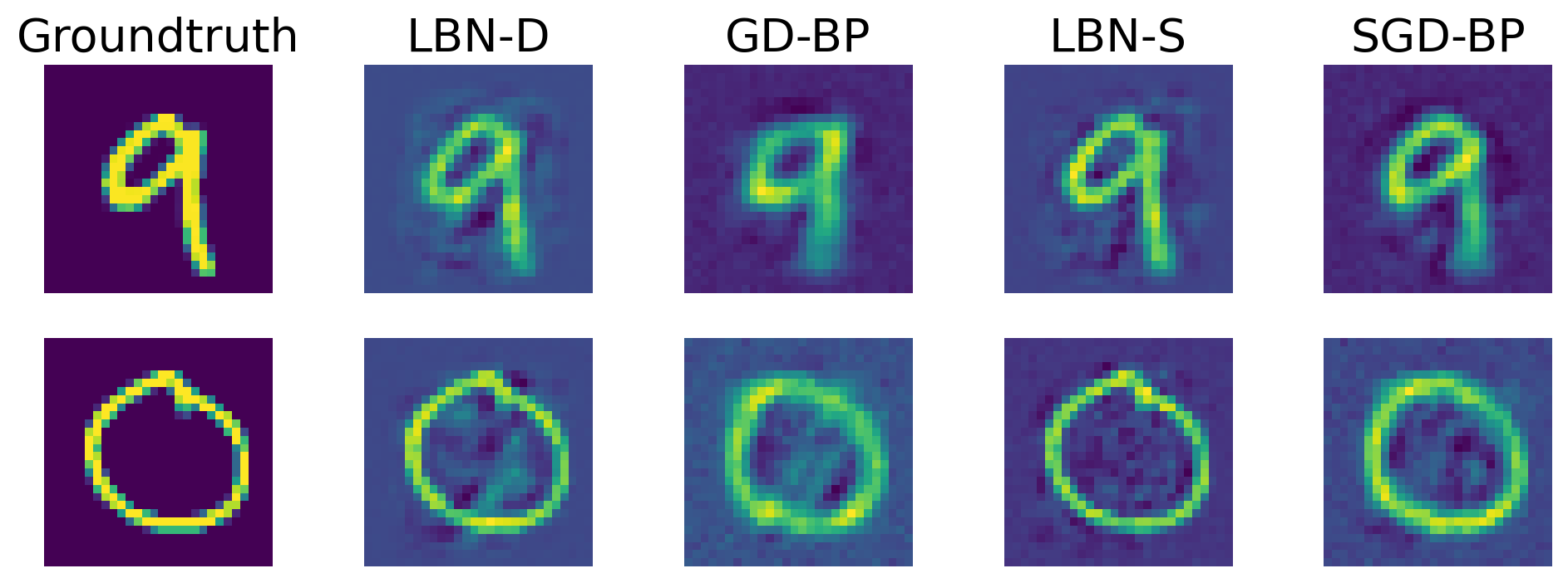
Figure 4: Reconstructed images from the MNIST training dataset for the LBN-D, LBN-S, GD-BP and SGD-BP training strategies respectively, along with ground truth images.

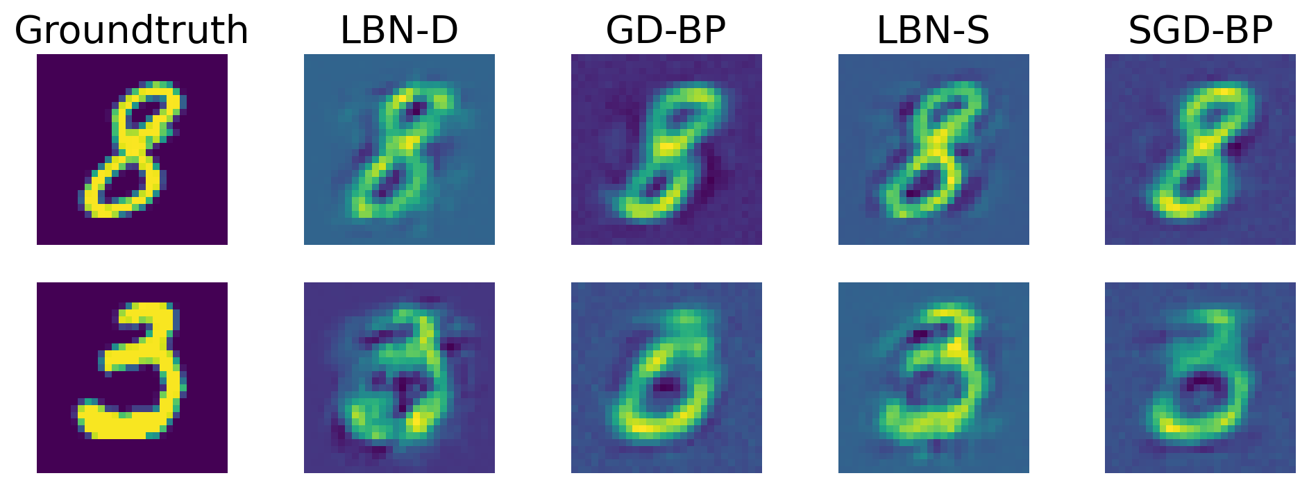
Figure 5: Reconstructed images from the MNIST validation dataset for the LBN-D, LBN-S, GD-BP and SGD-BP training strategies respectively, along with ground truth images.

6.3 Sparse Denoising Autoencoder

The sparse denoising autoencoder adopts the same network architecture as the sparse autoencoder described in Section 6.2, which sets the hidden dimension to 784 across all layers. To produce noisy images, instances of Gaussian random variables with mean zero and standard deviation $10^{-3}$ are added to each pixel. We use the MSE as the last layer loss function to measure the difference of reconstruction and noisy images. We consider two training scenarios to evaluate model performances: 1) In the first scenario, we train the network with limited data from the Fashion-MNIST dataset, similar to Section 6.2, where we take 1,000 training images (referred to as Fashion-MNIST-1K) and validate on 10,000 images. 2) For the second scenario, the training dataset consists of 10,000 images (referred to as Fashion-MNIST-10K) and the validation dataset consists of 10,000 images.
Fashion-MNIST-1K In the first group of experiments, we train a sparse autoencoder with imposed sparsity regularisation during training on the Fashion-MNIST-1K dataset. For the lifted Bregman training approach (LBN) we apply Algorithm 1 to minimise the learning objective (27) with $\alpha=0.09$. We set the batch size to $|B_{k}|=20$, the step-size parameter $\tau_{k}$ to $\tau_{k}=0.5$, for all $k$, and the inner iterations $N$ to $N=15$ for solving each mini-batch sub-problem (24) via (17). For comparison, we consider a vanilla stochastic (sub-)gradient method (SGD-BP) as described in (20) and the stochastic (sub-)gradient descent approach with implicit parameter update (ISGD-BP) that follows (22) to train the network parameters. Both approaches use the learning rate $1\times 10^{-3}$ and apply the back-propagation Algorithm 2 for computing the (sub-)gradients. The ISGD-BP does so by solving the inner problem with GD-BP for $N$ iterations.

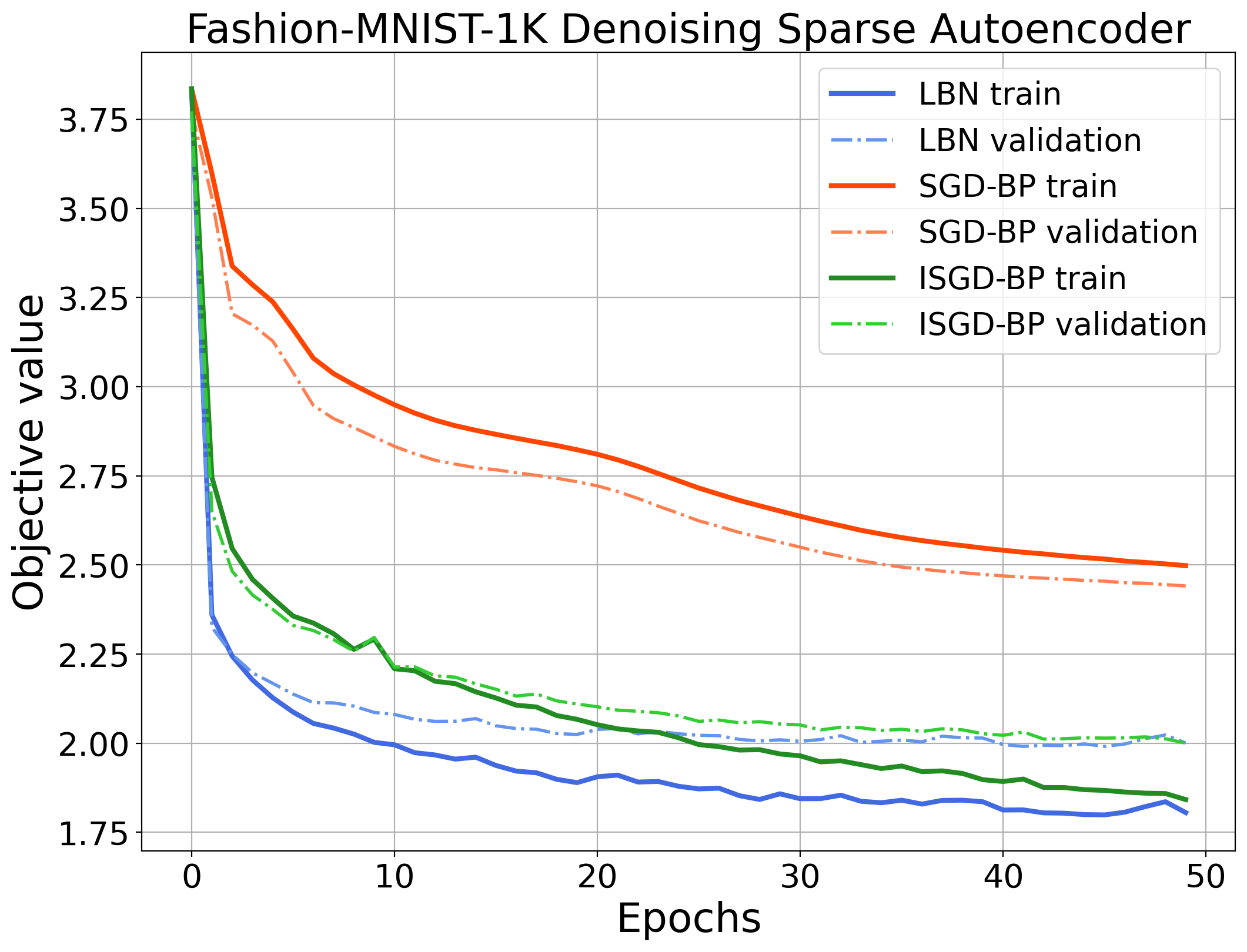
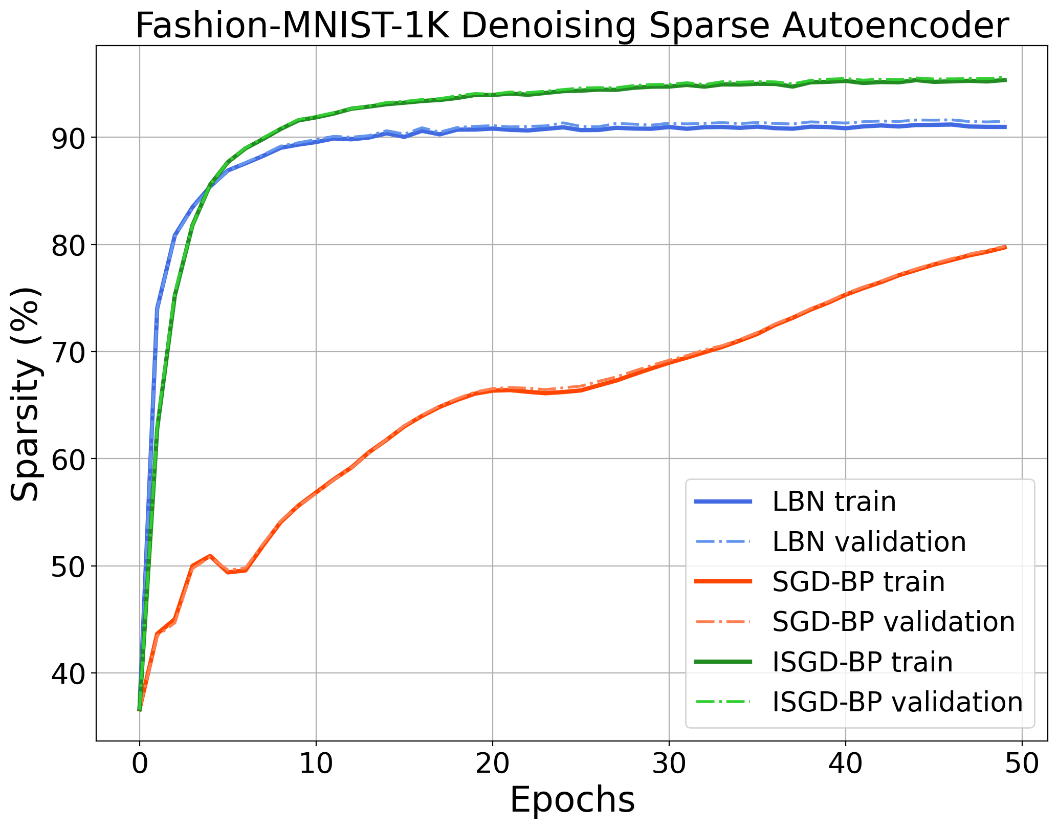
Figure 6: Sparse denoising autoencoder trained on Fashion-MNIST-1K images. Left: Objective values per epoch for each learning approach. The training loss record MSE reconstruction error plus $\alpha$ times $\ell_{1}$-norm regularisation while the validation loss record the MSE reconstruction error. Right: Sparsity level of the code per training epoch for each learning scheme.

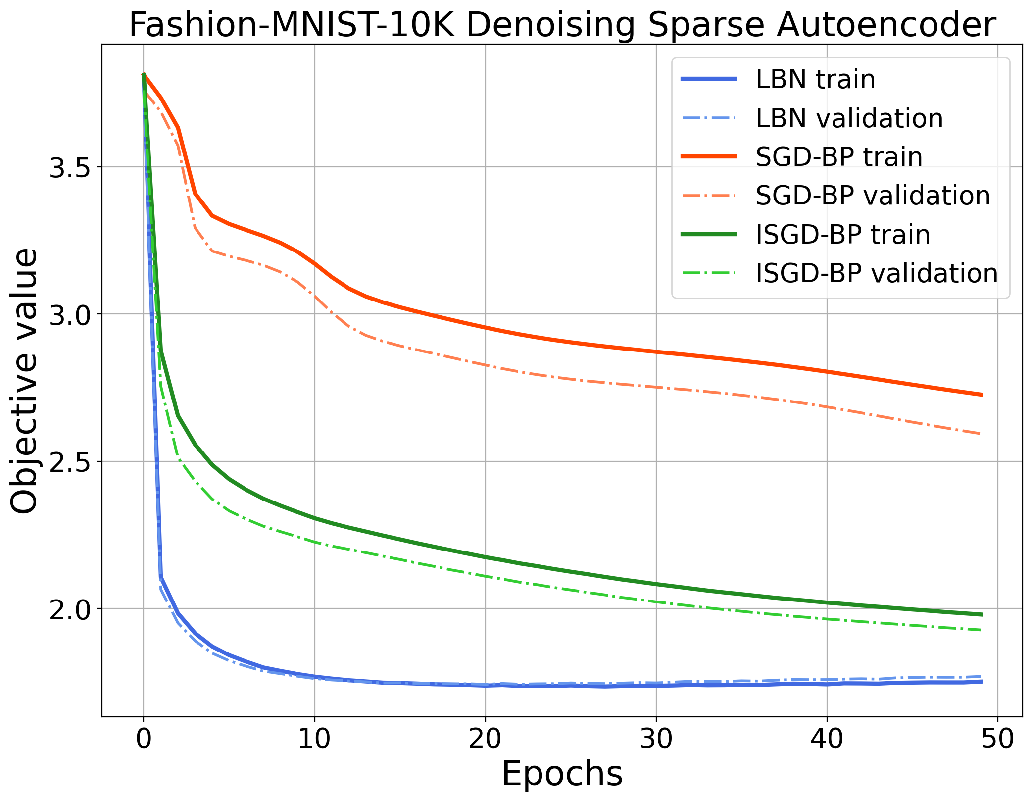
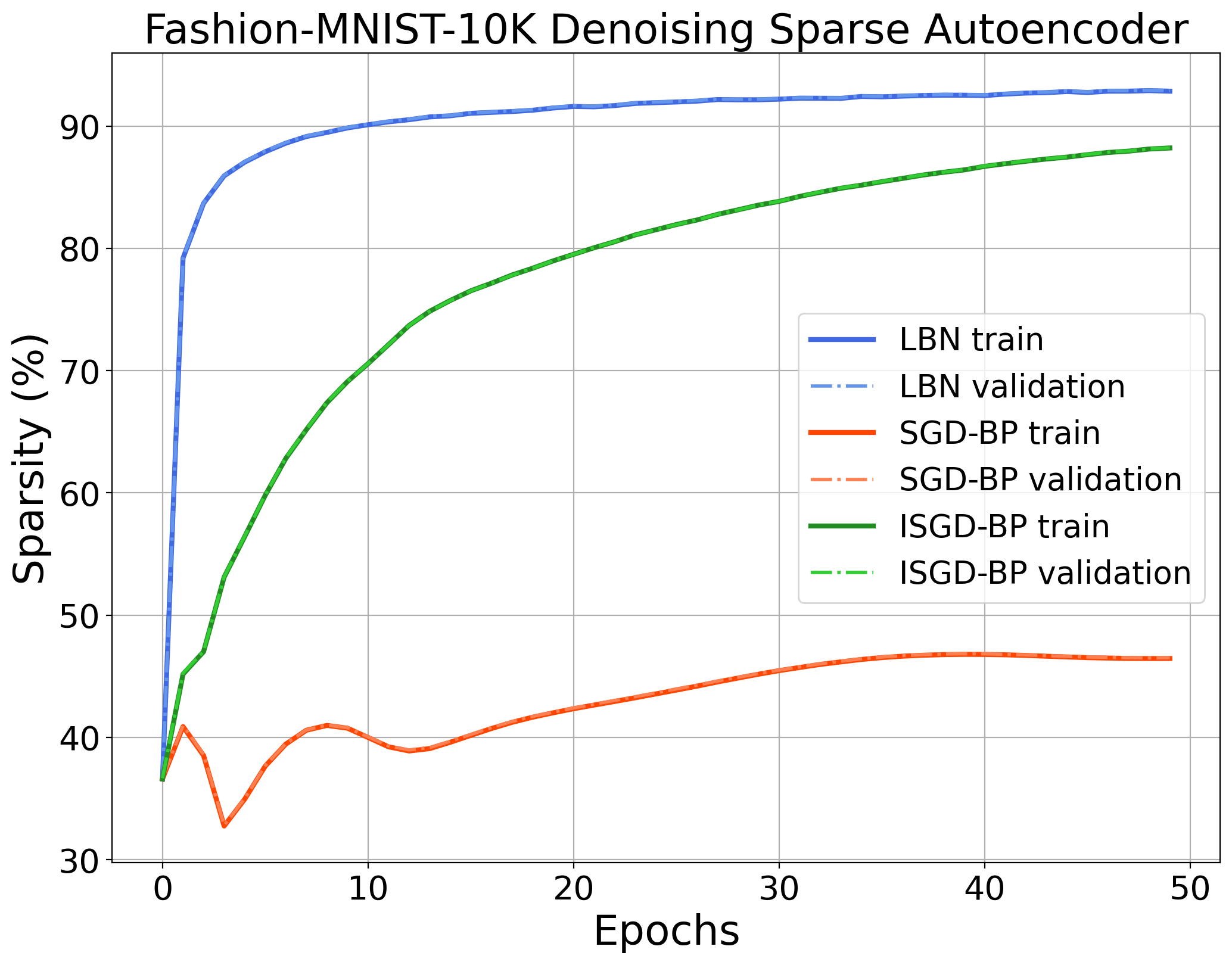
Figure 7: Sparse denoising autoencoder trained on the Fashion-MNIST-10K images. Left: Objective values per epoch for each learning approach. The training loss record MSE reconstruction error plus $\alpha$ times $\ell_{1}$-norm regularisation while validation loss curves record the MSE reconstruction error. Right: Sparsity level of the code over the 50 training epochs for each learning scheme.

All approaches train for 50 epochs. A log-scale plot of the objective value decay for all three training approaches is visualised in Figure 7 (Left) and the tracked changes of the hidden node sparsity level are plotted in Figure 7 (Right).

When trained on the Fashion-MNIST-1K dataset, we observe that LBN achieves faster convergence and outperforms ISGD-BP and SGD-BP especially at early training epochs. Towards later epochs, ISGD-BP starts to align and eventually achieves comparable training and validation errors.

The ISGD-BP approach and LBN approach are capable of achieving and maintaining higher sparsity levels from earlier epochs onwards, while the SGD-BP approach on the other hand seems to increase the sparsity level much more slowly compared to the other two approaches. It should, however, be emphasised that the SGD-BP algorithm is computationally less expensive per epoch.

Fashion-MNIST-10K We conduct the second set of experiments on the Fashion-MNIST-10K dataset. We choose a bigger batch size of $|B_{k}|=200$ and penalise the $\ell_{1}$-norm regularisation with $\alpha=0.055$ during training. For both the LBN and the ISGD-BP approach, we set $\tau_{k}=1$ and perform $N=30$ iterations in each mini-batch sub-problem. We choose a learning rate of $4\times 10^{-4}$ for the ISGD-BP approach as well as for the SGD-BP approach.

In Figure 7 we visualise the training and validation loss curves (Left) and the sparsity rate (Right) over the 50 training epochs when training the proposed algorithms on the Fashion-MNIST-10K dataset. As expected, the gap between training and validation loss curves in this experiment are closer due to larger amount of training samples while network complexity is unchanged. Note that the proposed LBN approach exhibits stronger performance and outperforms the other two (sub-)gradient based methods when a larger amount of training data is available. Not only is the LBN approach capable of achieving lower reconstruction loss values after 50 epochs but also achieves and maintains higher sparsity rates more quickly.

As both the LBN and ISGD-BP approach require 30 inner iterations per batch sub-problem, we also compare both approaches to the SGD-BP approach for 1500 epochs to ensure that the total number of iterations for all three approaches are comparable. As visualised in Figure 8, we verify with fairer comparison with regards to runtime that the SGD-BP approach matches training and validation errors of ISGD-BP, but falls short of achieving training and validation values as low as those obtained with LBN.

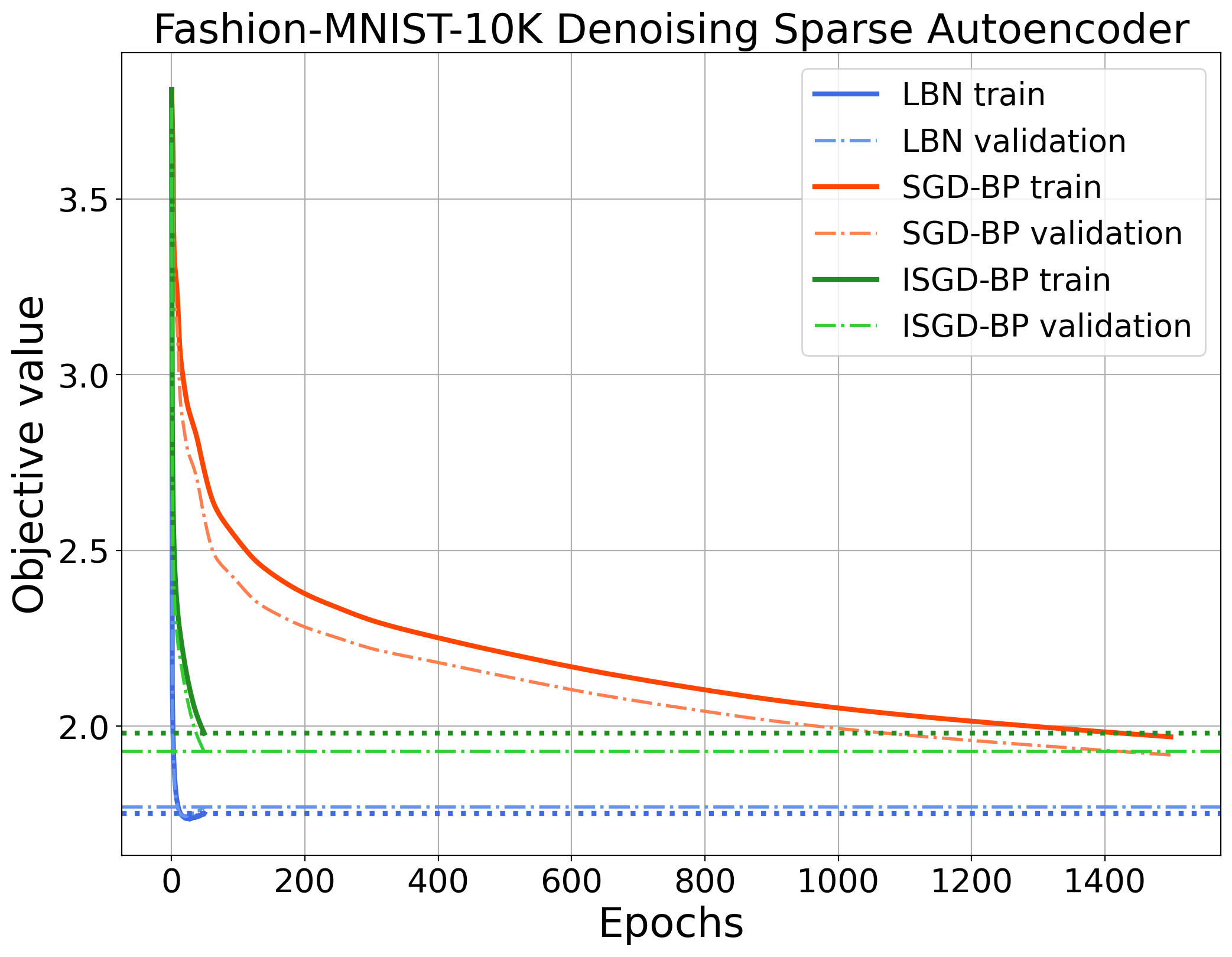
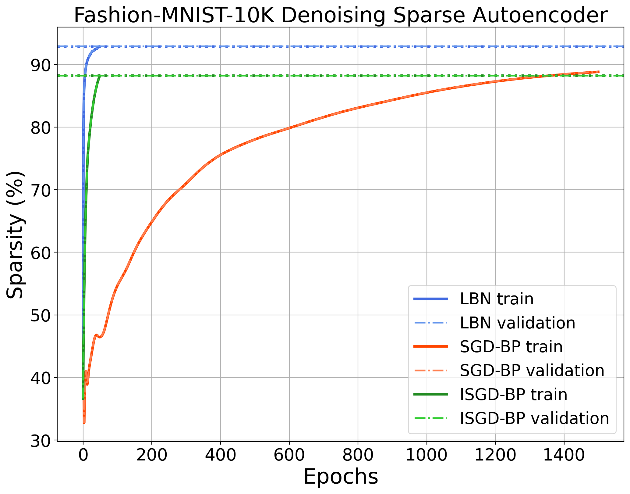
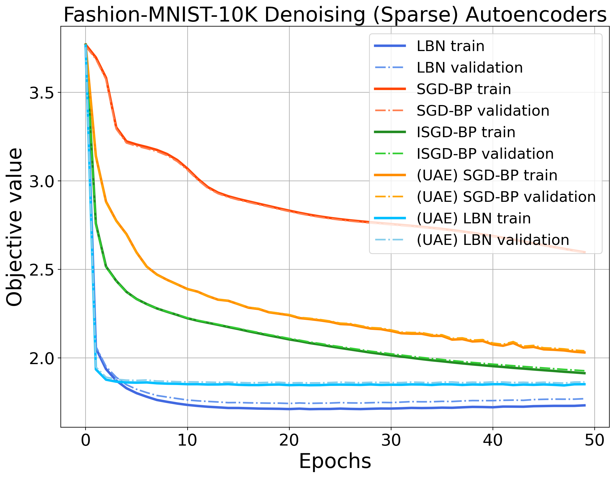
Figure 8: Comparison of sparse denoising autoencoders trained on the Fashion-MNIST-10K dataset with LBN, ISGD-BP and SGD-BP for 1500 epochs, and of sparse denoising autoencoders with undercomplete autoencoders. Left: Objective values per epoch for all learning approaches. Horizontal lines mark end-of-training and end-of-validation objective values of LBN and ISGD-BP. Middle: Sparsity level of the code over the 1500 training epochs. Horizontal lines show end-of-training sparsity rates of LBN and ISGD-BP. Right: Objective values per epoch for each learning approach. The training and validation loss curves report MSE reconstruction errors over 50 epochs.

Comparison with undercomplete autoencoders. So far, we haven’t properly motivated the use of sparse autoencoders in comparison to traditional autoencoders that explicitly reduce the dimension of the code. A sparse code with $m$ non-zero entries requires basically the same amount of memory than a $m$-dimensional code but offers greater flexibility because the location of the non-zero entries can vary for different network inputs. This advantage should lead to better validation errors of sparse autoencoders compared to traditional, undercomplete autoencoders. In order to verify the advantages of training sparse autoencoders over training undercomplete autoencoders (UAE), we conduct two additional experiments where we train undercomplete autoencoders on the Fashion-MNIST-10K dataset without imposing any additional regularisation.

We observe that the sparse denoising autoencoder trained with $\alpha=0.055$ eventually reaches 91% sparsity rate after 50 epchs, which suggests that on average 70 nodes in the code of the final model are activated. Hence, we train a 4-layer fully connected undercomplete autoencoder with ReLU activation function for every layer but set the number of nodes in the middle layer to 70, which implies $W_{2}\in\mathbb{R}^{784\times 70}$ and $W_{3}\in\mathbb{R}^{70\times 784}$. The undercomplete autoencoder is trained with both LBN and SGD-BP and we compare if a reconstruction quality comparable to the sparse autoencoder can be achieved.

In Figure 8, we validate that the lifted Bregman approach helps to improve both undercomplete and sparse autoencoder to achieve faster convergence and lower objective values compared to the (sub-)gradient based methods. We also confirm that after 50 epochs the sparse denoising autoencoder achieves lower training and validation errors compared to the UAE approach.

More specifically, the UAE model trained with the lifted Bregman approach sees bigger reconstruction loss decreases in the early epochs, but is outperformed by the sparse autoencoder at later epochs. This experiment seems to suggest that by leveraging the power of sparsity, sparse autoencoders trained via lifted Bregman approaches are capable of finding more flexible data representations compared to autoencoders with explicit dimension reduction.

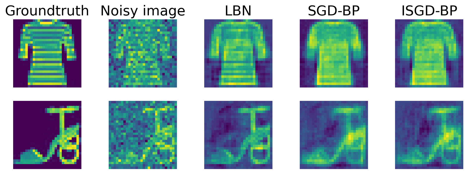
Figure 9: Denoised images from the Fashion-MNIST-1K training dataset, computed with the LBN, the SGD-BP and the ISGD-BP training strategies for 50 epochs, along with the noise-free and noisy images.

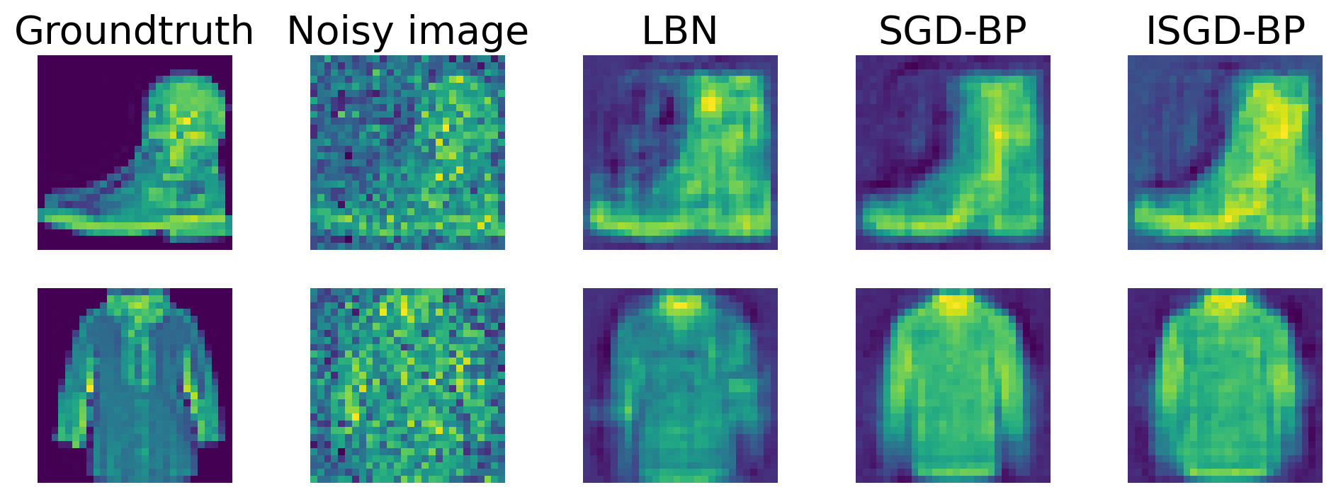
Figure 10: Denoised images from the Fashion-MNIST-1K validation dataset computed with the LBN, the SGD-BP and the ISGD-BP training strategies for 50 epochs, along with the noise-free and noisy images.

We visualise a selection of denoised sample images from the Fashion-MNIST-1K training dataset in Figure 10 and from the Fashion-MNIST-10K training dataset in Figure 12. Although the loss values of LBN and ISGD-BP were comparable after 50 epochs, the visual comparison between the network outputs suggests that the network trained with LBN is able to restore finer details (for instance the stripes on the t-shirt).

The same network also exhibits better denoising performance for the validation images as seen in Figure 10.

Similar observations can be made when we examine denoised sample images from the models trained on the Fashion-MNIST-10K dataset (Figure 12). The LBN trained network is capable of recovering fine structures such as the dotted backpack object. Both SGD-BP and ISGD-BP struggle with fine details and are prone to producing coarse approximations. The observations still hold true for the validation dataset as can be seen from Figure 12. For example, the LBN approach is able to recover the curvature of the trousers, but SGD-BP and ISGD-BP only recover straight-legged trousers.

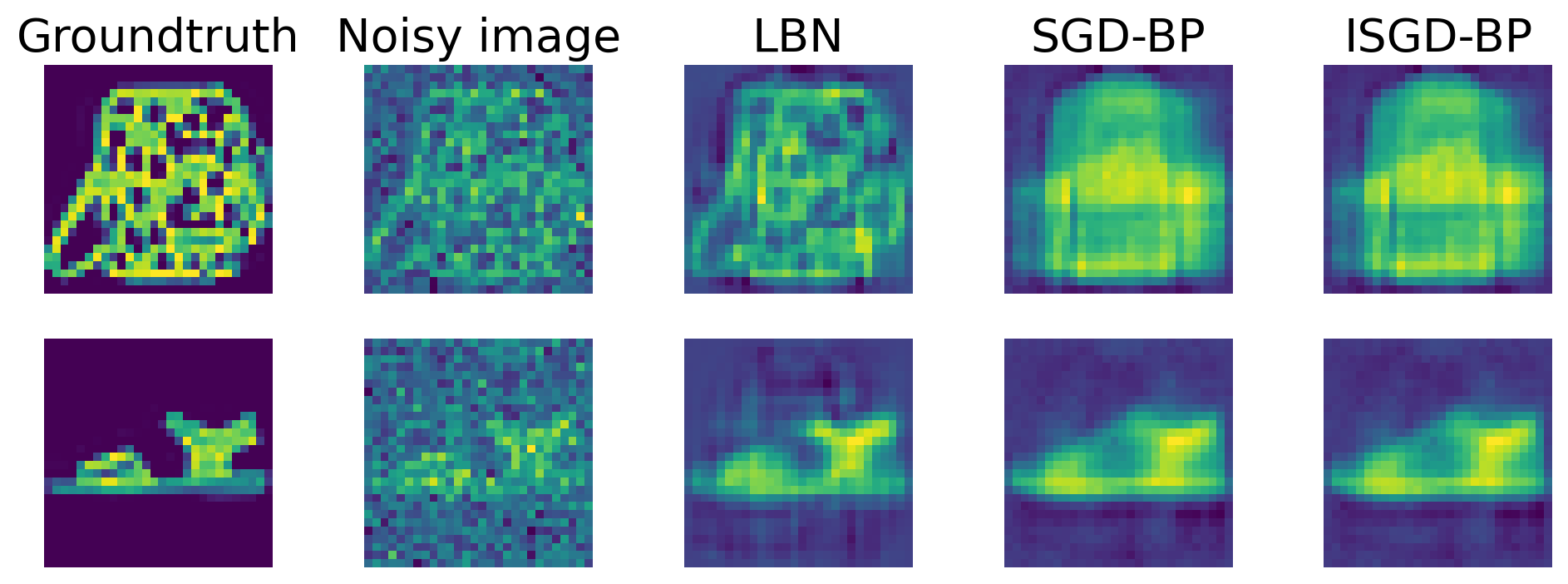
Figure 11: Denoised images from the Fashion-MNIST-10K training dataset computed with the LBN, the SGD-BP (trained for 1500 epochs) and the ISGD-BP training strategies respectively, along with the noise-free and noisy images.

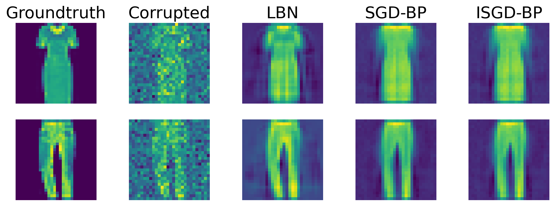
Figure 12: Denoised images from the Fashion-MNIST-10K validation dataset computed with the LBN, the SGD-BP (trained for 1500 epochs) and the ISGD-BP training strategies respectively, along with the noise-free and noisy images.

7 Conclusions & outlook

In this work, we proposed a novel framework for learning parameters of feed-forward neural networks. To achieve that, we introduced a new loss function based on Bregman distances and we provided a detailed mathematical analysis of this new loss function. By replacing the quadratic penalties in the MAC-QP approach, we generalised MAC-QP and lifted network frameworks as introduced in (Carreira-Perpinan and Wang, 2014; Askari et al., 2018; Li et al., 2019; Gu et al., 2020) and established rigorous mathematical properties.

The advantage of the proposed framework is that it formulates the training of a feed-forward network as a minimisation problem in which computing partial derivatives of the network parameters does not require differentiation of the activation functions. We have demonstrated that this framework can be realised computationally with a variety of different deterministic and stochastic minimisation algorithms.

With numerical experiments in classification and compression, we compared the implementation of the proposed framework with proximal gradient descent and implicit stochastic gradient method to explicit and implicit stochastic gradient methods with back-propagation.

For classification, we have shown that the trained network is fully non-linear in contrast to the lifted network approach proposed in Askari et al. (2018), while also achieving similar classification accuracy as networks trained with first- order methods with back-propagation.

For compression, we showed with our sparse autoencoder example that training parameters with proximal gradient descent or implicit stochastic gradient descent can be more efficient than first-order methods with back-propagation. We have also shown that it is straightforward to integrate regularisation acting on the activation variables. This enabled us to design an autoencoder with sparse codes that is shown to produce more adaptive compressions compared to conventional autoencoders.

There are many possible directions for future work. In this work, the proposed concept is limited to feed-forward neural network architectures, but it can easily be extended to other types of architectures such as residual neural networks (He et al., 2016). Residual networks of the form $x_{l+1}=x_{l}-\sigma(f(x_{l},\Theta_{l}))$ can for instance be trained with a slight modification of (13) in the form of

$$\min_{\mathbf{\Theta},\mathbf{X}}\sum_{i=1}^{s}\left[\ell\left(y^{i},x_{L}^{i}\right)+\sum_{l=1}^{L-1}\,\lambda_{l}B_{\Psi}\left(x_{l}^{i}-x_{l-1}^{i},f(x_{l-1}^{i},\Theta_{l})\right)\right]\,,$$

and many modifications with different linear transformations of the auxiliary variables.

Other notable research directions include feasibility studies on how to incorporate other popular layers, such as pooling layers, batch normalisation layers (Ioffe and Szegedy, 2015; Ba et al., 2016), or transformer layers (Vaswani et al., 2017), the application of other optimisation methods such as stochastic coordinate descent, stochastic ADMM, or stochastic primal-dual hybrid gradient methods as well as tailored non-convex optimisation methods and other regularisation techniques like dropout Hinton et al. (2012).

Similar to suggestions made in Zach and Estellers (2019), we could use the network energy for anomaly detection. As our proposed framework has opened more pathways to use other possible combinations of optimisation strategies, it would also be of particular interest to investigate more thoroughly if good generalisation properties of a deep neural network are the result of the chosen optimisation strategy or the chosen network architecture itself.

Appendix A Back-propagation

Algorithm 2 Back-Propagation Algorithm

  Input $\mathbf{\Theta}$  

  for $i=1,\ldots,s$ do

     for $l=1,\ldots,L$ do

        Perform forward pass to compute $z_{l}$ and $x_{l}$:

        $z_{l}^{i}=f(x_{l-1}^{i},\Theta_{l})$

        $x_{l}^{i}=\sigma_{l}(z_{l}^{i})$

     end for

  end for

  for $i=1,\ldots,s$ do

     for $l=L,\ldots,1$ do

        Perform backward pass to compute $\delta_{l}^{i}$:

        $\delta_{l}^{i}=\begin{cases}\sigma_{l}^{\prime}(z_{L}^{i})\odot\nabla_{x}\ell(y^{i},x_{L}^{i})\;\;\;\text{for }l=L\\ \sigma_{l}^{\prime}(z_{l}^{i})\odot\frac{\partial f}{\partial x_{l}}\delta_{l+1}\;\;\;\text{for }l\in\{1,\ldots,L-1\}\\ \end{cases}$

     end for

  end for

  Partial derivatives: $\frac{\partial\ell}{\partial\Theta_{l}^{jk}}=\delta_{l}^{j}\frac{\partial f}{\partial\Theta_{l}^{k}}\;\;\;\text{for }j\in\{1,\ldots,n_{l}\}\text{ and }k\in\{1,\ldots,n_{l-1}\}$

We can write down the corresponding Lagrangian function for (5) as

$$\mathcal{L}(\mathbf{\Theta},\mathbf{X},\mathbf{Z},\mu,\delta)=\sum_{i=1}^{s}\left[\ell(y,x_{L}^{i})+\sum_{l=1}^{L}\langle\mu_{l}^{i},x_{l}^{i}-\sigma(z_{l}^{i})\rangle+\sum_{l=1}^{L}\langle\delta_{l}^{i},z_{l}^{i}-f(x_{l-1}^{i},\Theta_{l})\rangle\right]\,,$$ (28)

where $\mu=\{\mu_{l}^{i}\}_{l=1,\dots,L}^{i=1,\dots,s}$ and $\delta=\{\delta_{l}^{i}\}_{l=1,\dots,L}^{i=1,\dots,s}$ are Lagrangian multipliers.

In the following deduction of the back-propagation algorithm, we fix for one training data sample and drop the dependency on $i$ for the ease of notation. The optimality conditions of (28) can be split into the following sub-conditions:

$$\frac{\partial\mathcal{L}}{\partial x_{L}}=0\implies\nabla_{x_{L}}\ell(y,x_{L})+\mu_{L}=0\;\;$$ (29)

$$\frac{\partial\mathcal{L}}{\partial\Theta_{l}}=0\implies\delta_{l}=\frac{\partial f}{\partial\Theta_{l}}\mu_{l}^{\top}\;\;\text{for }l=1,\ldots L-1$$ (30)

$$\frac{\partial\mathcal{L}}{\partial x_{l}}=0\implies\mu_{l}=\frac{\partial f}{\partial x_{l}}\delta_{l+1}\;\;\text{for }l=1,\ldots L-1$$ (31)

$$\frac{\partial\mathcal{L}}{\partial z_{l}}=0\implies\delta_{l}=\sigma_{l}^{\prime}(z_{l})\mu_{l}\;\;\text{for }l=1\ldots L$$ (32)

$$\frac{\partial\mathcal{L}}{\partial\mu_{l}}=0\implies x_{l}=\sigma_{l}(f(x_{l-1},\Theta_{l}))\;\;\text{for }l=1,\ldots L$$ (33)

$$\frac{\partial\mathcal{L}}{\partial\delta_{l}}=0\implies z_{l}=f(x_{l-1},\Theta_{l})\;\;\text{for }l=1,\ldots L$$ (34)

Notice that sub-conditions (33) and (34) carry out exactly the forward-pass of the Algorithm 2. Merging sub-conditions (31) and (32) gives

$$\delta_{l}=\sigma_{l}^{\prime}(z_{l})\frac{\partial f}{\partial x_{l}}\delta_{l+1}\;\;\text{for }l=1\ldots L-1\,\,,$$

which is the backward-pass in Algorithm 2 for computing the partial derivatives. Sub-conditions (29) and (30) on the other hand are computational steps for taking the (sub-)gradient update step (cf. Higham and Higham (2019)).

A.1 Related works

To tackle the major limitations of the classical lifted training approach, several other recent works also formulate training of lifted networks differently. Fenchel lifted neural network (Gu et al., 2020) and Lifted Proximal Operator Machine (LPOM) (Li et al., 2019) both extend the observation in Zhang and Brand (2017) to a broader class of activation functions and demonstrate improved learning performance. In this section, we briefly present the approaches proposed in these works and point out the their connections and differences to the proposed lifted Bregman framework.

Fenchel lifted neural networks (Gu et al., 2020) extend the classical lifted network approach (Askari et al., 2018) as discussed in Section 2.3.2 by reformulating the learning problem (2) of a neural network with affine-linear function $f(x_{l-1},\Theta_{l})=W_{l}^{\top}x_{l-1}+b_{l}$ as

$$\min_{\mathbf{X},\{W_{l},b_{l}\}_{l=1}^{L}}\;\;\sum_{i=1}^{s}\ell(y^{i},W_{L}^{\top}x_{L-1}^{i}+b_{L})$$

$$\text{\;\;\;\;\;\;\;s.t. }B_{l}(x_{l},W_{l}^{\top}x_{l-1}^{i}+b_{l})\leq 0\,,\;\text{for}\;l=0\ldots L-1\,.$$

where the equality constraints in Problem (5) are converted into constraints on a collection of pre-defined biconvex functions $B_{l}$. For one fixed data pair $(x,y)$, the constraint $B_{l}(x_{l},W_{l}^{\top}x_{l-1})\leq 0$ provides the characterisation of an activation function via

$$x_{l}^{i}=\sigma(W_{l}^{\top}x_{l-1}^{i}+b_{l})\qquad\Leftrightarrow\qquad B_{l}(x_{l}^{i},W_{l}^{\top}x_{l-1}^{i}+b_{l})\leq 0\,.$$

The Lagrange formulation of the constrained minimisation problem yields

$$\min_{\mathbf{X},\{W_{l},b_{l}\}_{l=1}^{L}}\;\;\sum_{i=1}^{s}\left[\ell(y^{i},W_{L}^{\top}x^{i}_{L-1})+\sum_{l=1}^{L}\lambda_{l}B_{l}(x_{l+1},W_{l+1}^{\top}x_{l})\right]\,\,,$$

where $\lambda_{l}$ are the Lagrange multipliers. The bi-convex functions $B_{l}$ essentially take on the same role as the Bregman loss function (12), but without making the connection to Bregman distances and without many of the theoretical results provided in this paper. In the case of the ReLU activation function $\sigma(z)=\max(z,0)$, the functions $B_{l}$ are defined as

$$B_{l}(v,u) =\begin{cases}\frac{1}{2}v^{2}+\frac{1}{2}u_{+}^{2}-uv&\text{if }v\geq 0\\ \infty&\text{otherwise}\end{cases}\,.$$

Using Item 4 in Theorem 10, it is not difficult to see that this is the scalar-valued equivalent of the Bregman loss function

$$B_{\Psi}(x,z) =\begin{cases}\frac{1}{2}\|x\|^{2}+\frac{1}{2}\|\max(z,0)\|^{2}-\langle z,x\rangle&\text{if }x\geq 0\\ \infty&\text{otherwise}\end{cases}\,.$$

However, without using generalised Bregman distances and proximal activation functions, the derivation of $B_{l}$ in Gu et al. (2020) requires deducing the energy from the optimality system. Further, derivations for activation functions other than ReLU seem possible but not as straightforward. Moreover, the analysis in Gu et al. (2020) requires the activation function $\sigma$ to be strictly monotone, while such strong restrictions are not required in this work.

LPOM on the other hand takes a similar approach to Gu et al. (2020) through the use of proximal operators. The authors define

$$f(x):=\int_{0}^{x}(\sigma^{-1}(y)-y)dy\qquad\text{and}\qquad g(x):=\int_{0}^{x}(\sigma(y)-y)dy$$

such that the proximal map of $f$ as defined in Definition 1 is $\sigma$, and the proximal map of $g$ is $\sigma^{-1}$. The authors of Li et al. (2019) propose to approximate (5) with

$$\min_{\mathbf{X},\{W_{l},b_{l}\}_{l=1}^{L}}\;\;\sum_{i=1}^{s}\ell(y^{i},W_{L}^{\top}x^{i}_{L-1}+b_{L})+\sum_{l=1}^{L-1}\mu_{l}(f(x_{l}^{i})+g(W_{l}^{\top}x_{l-1}^{i})+\frac{1}{2}\|x_{l}^{i}-(W_{l}^{\top}x_{l-1}^{i}+b_{l})\|^{2})\,,\\$$

such that the optimality condition of the objective with respect to $x_{l}^{i}$ reads

$$0=\mu_{l}(\sigma^{-1}(x_{l}^{i})-(W_{l}^{\top}x_{l-1}^{i}+b_{l}))+\mu_{l+1}(W_{l+1})(\sigma(W_{l+1}^{\top}x_{l}^{i}+b_{l})-x_{l+1}^{i})\,\,\,.$$

Similar to the proposed approach, this approach ensures that the network constraints $x_{l}^{i}=\sigma(W_{l}^{\top}x_{l-1}^{i}+b_{l})$ are satisfied. However, like the Fenchel lifted neural network network approach, the LPOM work requires more restrictive assumptions such as invertibility of the activation function $\sigma$, and provides fewer mathematical insights into the newly defined penalisation functions.

Appendix B Numerical realisation

In this section we present two other suitable deterministic strategies for the computational minimisation of (13).

B.1 Coordinate descent

The function $E$ in Section 4 is convex in each individual variable if all other variables are kept fixed. It therefore makes sense to consider alternating minimisation approaches, also known as coordinate descent, for the minimisation of $E$, i.e.

$$\Theta_{l}^{k+1} =\operatorname*{\arg\min}_{\Theta_{l}}E\left(\Theta_{1}^{k+1},\ldots,\Theta_{l-1}^{k+1},\Theta_{l},\Theta_{l+1}^{k},\ldots,\Theta_{L},x_{1}^{k},\ldots,x_{L-1}^{k}\right)\,,$$ (35a)

respectively

$$x_{j}^{k+1} =\operatorname*{\arg\min}_{x_{j}}E\left(\Theta_{1}^{k+1},\ldots,\Theta_{L}^{k+1},x_{1}^{k+1},\ldots,x_{j-1}^{k+1},x_{j},x_{j+1}^{k},\ldots,x_{L-1}^{k}\right)\,,$$ (35b)

for $l\in\{1,\ldots,L\}$ and $j\in\{1,\ldots,L-1\}$. Obviously, the order of updating the individual parameters is completely arbitrary and can be replaced with permutations. However, we want to point out that it does make sense to alternate with respect to the $\mathbf{\Theta}$ and $\mathbf{X}$ block, and to further alternate between the block of even and odd indices within the $\mathbf{X}$ block. Suppose $L$ is even, then this alternating optimisation between blocks can be written as

$$\mathbf{\Theta}^{k+1} =\operatorname*{\arg\min}_{\Theta_{1},\ldots,\Theta_{L}}E\left(\Theta_{1},\ldots,\Theta_{L},x_{1}^{k},\ldots,x_{L-1}^{k}\right)\,,$$ (36a)

$$\{x_{2l-1}^{k+1}\}_{l=1}^{\frac{L}{2}} =\operatorname*{\arg\min}_{x_{1},x_{3},\ldots,x_{L-1}}E\left(\Theta_{1}^{k+1},\ldots,\Theta_{L}^{k+1},x_{1},x_{2}^{k},x_{3},\ldots,x_{L-2}^{k},x_{L-1}\right)\,,$$ (36b)

$$\{x_{2l}^{k+1}\}_{l=1}^{\frac{L}{2}} =\operatorname*{\arg\min}_{x_{2},x_{4},\ldots,x_{L-2}}E\left(\Theta_{1}^{k+1},\ldots,\Theta_{L}^{k+1},x_{1}^{k+1},x_{2},x_{3}^{k+1},\ldots,x_{L-2},x_{L-1}^{k+1}\right)\,.$$ (36c)

This alternating scheme has the advantage that the individual optimisation problems are still convex, but whilst the three blocks have to be updated sequentially, every variable in each of the three blocks can be updated in parallel. This becomes evident if we write down the individual optimisation problems, i.e.

$$\Theta_{l}^{k+1}{}={} \operatorname*{\arg\min}_{\Theta_{l}}\left\{\left(\frac{1}{2}\|\cdot\|^{2}+\Psi\right)^{\ast}\left(f(x_{l-1}^{k},\Theta_{l})\right)-\left\langle x_{l}^{k},f(x_{l-1}^{k},\Theta_{l})\right\rangle\right\}\,,$$ (37a)

$$x_{i}^{k+1}{}={} \operatorname*{\arg\min}_{x_{i}}\left\{\left(\frac{1}{2}\|\cdot\|^{2}+\Psi\right)(x_{i})-\left\langle x_{i},f(x_{i-1}^{k},\Theta_{i}^{k+1})\right\rangle\right.$$ (37b)

$$\qquad\qquad\left.+\left(\frac{1}{2}\|\cdot\|^{2}+\Psi\right)^{\ast}\left(f(x_{i},\Theta_{i+1}^{k+1})\right)-\left\langle f(x_{i},\Theta_{i+1}^{k+1}),x_{i+1}^{k}\right\rangle\right\}\,,$$

$$x_{j}^{k+1}{}={} \operatorname*{\arg\min}_{x_{j}}\left\{\left(\frac{1}{2}\|\cdot\|^{2}+\Psi\right)(x_{j})-\left\langle x_{j},f(x_{j-1}^{k+1},\Theta_{j}^{k+1})\right\rangle\right.$$ (37c)

$$\qquad\qquad\left.+\left(\frac{1}{2}\|\cdot\|^{2}+\Psi\right)^{\ast}\left(f(x_{j},\Theta_{j+1}^{k+1})\right)-\left\langle f(x_{j},\Theta_{j+1}^{k+1}),x_{j+1}^{k+1}\right\rangle\right\}\,,$$

for $l\in\{1,\ldots,L\}$, $i\in\{1,3,\ldots,L-1\}$ and $j\in\{2,4,\ldots,L-2\}$.

Note that the individual updates in (35) and in (36), respectively (37), are still implicit. If we, for instance, want to make the updates with respect to $\Theta$ explicit, we can modify (35a) to

$$\Theta_{l}^{k+1}=\operatorname*{\arg\min}_{\Theta_{l}}\left\{E\left(\Theta_{1}^{k+1},\ldots,\Theta_{l-1}^{k+1},\Theta_{l},\Theta_{l+1}^{k},\ldots,\Theta_{L},x_{1}^{k},\ldots,x_{L-1}^{k}\right)\right.$$ (38)

$$\left.+D_{J}\left(\left(\Theta_{1}^{k+1},\ldots,\Theta_{l-1}^{k+1},\Theta_{l},\Theta_{l+1}^{k},\ldots,\Theta_{L}^{k}\right),\left(\Theta_{1}^{k+1},\ldots,\Theta_{l-1}^{k+1},\Theta_{l}^{k},\Theta_{l+1}^{k},\ldots,\Theta_{L}^{k}\right)\right)\right\}\,,$$

where $D_{J}$ denotes the Bregman distance w.r.t. the function $J(\mathbf{\Theta})=\sum_{l=1}^{L}\frac{1}{2\tau_{\Theta_{l}}}\|\Theta_{l}\|^{2}-E(\mathbf{\Theta},\mathbf{X}^{k})$. Similar modifications can be deployed for the block-coordinate descent scheme (36), respectively (37), and the auxiliary parameters $\mathbf{X}$. In Appendix B.2, we briefly address how to computationally solve the individual sub-problems (37a), (37b) and (37c), with a special case of alternating minimisation approach: the alternating direction method of multipliers (ADMM), see Gabay (1983).

B.2 Alternating direction method of multipliers

In the previous section we have explored how to break the optimisation problem into different blocks via coordinate descent. Each of these blocks could be solved with proximal gradient descent as described in Section 4.1.1. However, we can alternatively solve these blocks with ADMM instead. Beginning with sub-problem (37a), we can introduce auxiliary variables $z_{l}=f(x_{l-1}^{k},\Theta_{l})$ to replace (37a) with the constrained formulation

$$(\Theta_{l}^{k+1},z_{l}){}={} \operatorname*{\arg\min}_{\Theta,z}\left\{\left(\frac{1}{2}\|\cdot\|^{2}+\Psi\right)^{\ast}\left(z\right)-\left\langle x_{l}^{k},z\right\rangle\right\}\quad\text{subject to}\quad z=f(x_{l-1}^{k},\Theta)\,,$$

for all $l\in\{1,\ldots,L\}$. By introducing Lagrange multipliers $\{\mu_{l}\}_{l=1}^{L}$, we can transform these problems into saddle-point problems of the form

$$(\Theta_{l}^{k+1},z_{l},\mu_{l}){}={} \operatorname*{\arg\min}_{\Theta,z}\max_{\mu}\left\{\left(\frac{1}{2}\|\cdot\|^{2}+\Psi\right)^{\ast}\left(z\right)-\left\langle x_{l}^{k},z\right\rangle+\left\langle\mu,z-f(x_{l-1}^{k},\Theta)\right\rangle\right\}\,.$$

ADMM computationally solves this saddle-point problem by alternatingly minimising and maximising the associated augmented Lagrangian

$$\mathcal{L}_{l}^{k}(\Theta,z;\mu)=\left(\frac{1}{2}\|\cdot\|^{2}+\Psi\right)^{\ast}\left(z\right)-\left\langle x_{l}^{k},z\right\rangle+\left\langle\mu,z-f(x_{l-1}^{k},\Theta)\right\rangle+\frac{\delta_{l}}{2}\left\|z-f(x_{l-1}^{k},\Theta)\right\|^{2}\,,$$

for a positive parameter $\delta_{l}$, i.e.

$$\Theta_{l}^{j+1} =\operatorname*{\arg\min}_{\Theta}\mathcal{L}_{l}^{k}(\Theta,z_{l}^{j};\mu_{l}^{j})\,,$$

$$z_{l}^{j+1} =\operatorname*{\arg\min}_{z}\mathcal{L}_{l}^{k}(\Theta_{l}^{j+1},z;\mu_{l}^{j})\,,$$

$$\mu_{l}^{j+1} =\operatorname*{\arg\max}_{\mu}\mathcal{L}_{l}^{k}(\Theta_{l}^{j+1},z_{l}^{j+1};\mu)-\frac{1}{2\delta_{l}}\|\mu-\mu_{l}^{j}\|^{2}\,.$$

In the context of (37a), these updates read

$$\Theta_{l}^{j+1} =\operatorname*{\arg\min}_{\Theta}\left\{\frac{\delta_{l}}{2}\left\|f(x_{l-1}^{k},\Theta)-z_{l}^{j}\right\|^{2}-\langle\mu_{l}^{j},f(x_{l-1}^{k},\Theta)\rangle\right\}\,,$$

$$z_{l}^{j+1} =\text{prox}_{\frac{1}{\delta_{l}}(\frac{1}{2}\|\cdot\|^{2}+\Psi)^{\ast}}\left(\frac{1}{\delta_{l}}\left(x_{l}^{k}-\mu_{l}^{j}+\delta_{l}\,f(x_{l-1}^{k},\Theta_{l}^{j+1})\right)\right)\,,$$

$$\mu_{l}^{j+1} =\mu_{l}^{j}+\delta_{l}\left(z_{l}^{j+1}-f(x_{l-1}^{k},\Theta_{l}^{j+1})\right)\,.$$

Please note that the proximal map $\text{prox}_{\frac{1}{\delta_{l}}(\frac{1}{2}\|\cdot\|^{2}+\Psi)^{\ast}}$ can easily be expressed via the extended Moreau decomposition (Beck, 2017, Theorem 6.45), i.e. $\delta_{l}\,\text{prox}_{\frac{1}{\delta_{l}}(\frac{1}{2}\|\cdot\|^{2}+\Psi)^{\ast}}(x/\delta_{l})=x-\text{prox}_{\delta_{l}(\frac{1}{2}\|\cdot\|^{2}+\Psi)}(x)$. We further know $\text{prox}_{\delta_{l}(\frac{1}{2}\|\cdot\|^{2}+\Psi)}(x)=\text{prox}_{\frac{\delta_{l}}{1+\delta_{l}}\Psi}(x/(1+\delta_{l}))$; hence, we observe

$$z_{l}^{j+1} =\text{prox}_{\frac{1}{\delta_{l}}(\frac{1}{2}\|\cdot\|^{2}+\Psi)^{\ast}}\left(\frac{1}{\delta_{l}}\left(x_{l}^{k}-\mu_{l}^{j}+\delta_{l}\,f(x_{l-1}^{k},\Theta_{l}^{j+1})\right)\right)\,,$$

$$=\frac{1}{\delta_{l}}\left(x_{l}^{k}-\mu_{l}^{j}+\delta_{l}\,f(x_{l-1}^{k},\Theta_{l}^{j+1})-\text{prox}_{\frac{\delta_{l}}{1+\delta_{l}}\Psi}\left(\frac{1}{1+\delta_{l}}\left(x_{l}^{k}-\mu_{l}^{j}+\delta_{l}\,f(x_{l-1}^{k},\Theta_{l}^{j+1})\right)\right)\right)\,,$$

which is why we can compute the update solely based on a scaled version of the proximal map of $\Psi$, which is the activation function of the neural network.

Example 4

In analogy to Example 3 we design a feed-forward network architecture with $\Psi=\chi_{\geq 0}$, implying $\text{prox}_{\Psi}(z)=\max(z,0)$, and $f(x,\Theta_{l})=W^{\top}_{l}x+b_{l}$, for $\Theta_{l}=(W_{l},b_{l})$. Computing a solution to (37a) via ADMM yields the algorithm

$$W_{l}^{j+1} =\left(x_{l-1}^{k}(x_{l-1}^{k})^{\top}\right)^{-1}x_{l-1}^{k}\left(z_{l}^{j}+\frac{1}{\delta_{l}}\mu_{l}^{j}-b_{l}^{j}\right)^{\top}\,,$$ (39)

$$b_{l}^{j+1} =z_{l}^{j}-\left(\frac{1}{\delta_{l}}\mu_{l}^{j}-(W_{l}^{j+1})^{\top}x_{l-1}^{k}\right)\,,$$

$$r_{l}^{j+1} =x_{l}^{k}-\mu_{l}^{j}+\delta_{l}\left((W_{l}^{j+1})^{\top}x_{l-1}^{k}+b_{l}^{j+1}\right)\,,$$

$$z_{l}^{j+1} =\frac{1}{\delta_{l}}\left(r_{l}^{j+1}-\,\text{prox}_{\frac{\delta_{l}}{1+\delta_{l}}\Psi}\left(\frac{r_{l}^{j+1}}{1+\delta_{l}}\right)\right)\,,$$

$$\mu_{l}^{j+1} =\mu_{l}^{j}+\delta_{l}\left(z_{l}^{j+1}-\left((W_{l}^{j+1})^{\top}x_{l-1}^{k}+b_{l}^{j+1}\right)\right)\,,$$

for $l\in\{1,\ldots,L\}$, $j\in\mathbb{N}$ and suitable initial values $b_{l}^{0}$, $z_{l}^{0}$ and $\mu_{l}^{0}$. It is important to point out that (39) is not well defined for only one sample because $x_{l-1}^{k}(x_{l-1}^{k})^{\top}$ is not invertible. However, we can overcome this issue by extending $E$ to include more samples, so that instead of requiring invertibility of $x_{l-1}^{k}(x_{l-1}^{k})^{\top}$, we require invertibility of $\sum_{i=1}^{s}x_{i,l-1}^{k}(x_{i,l-1}^{k})^{\top}$, which can be achieved if one has sufficiently distinctive samples. Or we can add the term $\frac{\tau}{2}\|W_{l}-W_{l}^{j}\|^{2}_{\text{Fro}}$ to the augmented Lagrangian, with a positive multiple $\tau$, which doesn’t affect the minimiser but guarantees that (39) is well-defined by adding a positive multiple of the identity matrix to $x_{l-1}^{k}(x_{l-1}^{k})^{\top}$, respectively $\sum_{i=1}^{s}x_{i,l-1}^{k}(x_{i,l-1}^{k})^{\top}$.

In similar fashion to solving (37a), we can also solve (37b) and (37c) via ADMM. Because (37b) and (37c) have identical structure but only different variables, we focus on (37b) without loss of generality. If we follow the same line-of-reasoning as before, the associated augmented Lagrangian reads

$$\mathcal{L}_{l}^{k}(x,z;\mu){}={} \left(\frac{1}{2}\|\cdot\|^{2}+\Psi\right)(x)-\left\langle x,f(x_{l-1}^{k},\Theta_{l}^{k+1})\right\rangle+\left(\frac{1}{2}\|\cdot\|^{2}+\Psi\right)^{\ast}(z)-\langle z,x_{l+1}^{k}\rangle$$

$$+\left\langle\mu,z-f(x,\Theta_{l+1}^{k+1})\right\rangle+\frac{\delta_{l}}{2}\left\|z-f(x,\Theta_{l+1}^{k+1})\right\|^{2}\,.$$

However, the challenge lies in the optimality condition for $x$, which even for fixed variables $z$ and $\mu$ doesn’t lead to a closed-form solution for $x$ (unless $\Psi$ is constant). Alternatively, we can introduce another variable $v$ with constraint $v=x$ and formulate

$$\mathcal{L}_{l}^{k}(x,v,z;\mu){}={} \left(\frac{1}{2}\|\cdot\|^{2}+\Psi\right)(x)-\left\langle x,f(x_{l-1}^{k},\Theta_{l}^{k+1})\right\rangle+\left(\frac{1}{2}\|\cdot\|^{2}+\Psi\right)^{\ast}(z)-\langle z,x_{l+1}^{k}\rangle$$

$$+\left\langle\mu,\left(\begin{matrix}z\\ v\end{matrix}\right)-\left(\begin{matrix}f(v,\Theta_{l+1}^{k+1})\\ x\end{matrix}\right)\right\rangle+\frac{\delta_{l}}{2}\left\|\left(\begin{matrix}z\\ v\end{matrix}\right)-\left(\begin{matrix}f(v,\Theta_{l+1}^{k+1})\\ x\end{matrix}\right)\right\|^{2}\,.$$

Alternatingly minimising and maximising this augmented Lagrangian yields the updates

$$x_{l}^{j+1} =\text{prox}_{\frac{1}{1+\delta_{l}}\Psi}\left(\frac{\delta_{i}v_{i}^{j}+(\mu_{l}^{j})_{2}+f(x_{l-1}^{k},\Theta_{l}^{k+1})}{1+\delta_{l}}\right)\,,$$

$$v_{l}^{j+1} =\operatorname*{\arg\min}_{v}\left\{\frac{\delta_{l}}{2}\left\|f(v,\Theta_{l+1}^{k+1})-z_{l}^{j}\right\|^{2}-\left\langle(\mu_{l}^{j})_{1},f(v,\Theta_{l+1}^{k+1})\right\rangle\right\}\,,$$

$$z_{l}^{j+1} =\text{prox}_{\frac{1}{\delta_{l}}(\frac{1}{2}\|\cdot\|^{2}+\Psi)^{\ast}}\left(f(v_{l}^{j+1},\Theta_{l+1}^{k+1})+\frac{1}{\delta_{l}}\left(x_{l+1}^{k}-(\mu_{l}^{j})_{1}\right)\right)\,,$$

$$\mu_{l}^{j+1} =\left(\begin{matrix}z_{l}^{j+1}\\ v_{l}^{j+1}\end{matrix}\right)-\left(\begin{matrix}f(v_{l}^{j+1},\Theta_{l+1}^{k+1})\\ x_{l}^{j+1}\end{matrix}\right)\,,$$

for all $l\in\{1,3,\ldots,L-1\}$.

B.3 Constrained optimisation

Note that it is not necessarily known a-priori how to choose the scalar parameters $\{\lambda_{l}\}_{l=1}^{L}$ in (13). Alternatively, we can also re-formulate the constrained problem formulation (5) to

$$\begin{split}&\min_{\mathbf{\Theta},\mathbf{X}}\sum_{i=1}^{s}\ell(y^{i},x_{L}^{i})\\ \text{subject to}\qquad&B_{\Psi}(x_{l}^{i},f(x_{l-1}^{i},\Theta_{l}))\leq 0\quad\text{for all }\,l\in\{1,\ldots,L-1\}\,,\end{split}$$ (40)

similar to Gu et al. (2020). Note that we can write (40) as

$$\min_{\mathbf{\Theta},\mathbf{X}}\sum_{i=1}^{s}\ell(y^{i},x_{L}^{i})+\sum_{l=1}^{L-1}\chi_{\leq 0}\left(B_{\Psi}(x_{l}^{i},f(x_{l-1}^{i},\Theta_{l}))\right)\,,$$

for the characteristic function $\chi_{\leq 0}$ over the non-positive orthant, which is equivalent to the Lagrange formulation

$$\min_{\mathbf{\Theta},\mathbf{X}}\sup_{\{\lambda_{l}\}_{l=1}^{L-1}}\sum_{i=1}^{s}\ell(y^{i},x_{L}^{i})+\sum_{l=1}^{L-1}\left[\lambda_{l}B_{\Psi}(x_{l}^{i},f(x_{l-1}^{i},\Theta_{l}))-\chi_{\geq 0}(\lambda_{l})\right]\,,$$ (41)

if we express $\chi_{\leq 0}$ in terms of its conjugate $\chi_{\geq 0}$. Albeit being concave in $\{\lambda_{l}\}_{l=1}^{L-1}$, the objective function is not convex in $\mathbf{\Theta},\mathbf{X}$ in general, which is why swapping $\min$ and $\sup$ will not necessarily lead to the same optimisation problem. Nevertheless, we could employ coordinate descent or alternating direction method of minimisation techniques. We could for example solve (41) with an alternating minimisation and proximal maximisation algorithm of the form

$$(\mathbf{\Theta}^{k+1},\mathbf{X}^{k+1}) \in\operatorname*{\arg\min}_{\mathbf{\Theta},\mathbf{X}}\left\{\sum_{i=1}^{s}\ell(y^{i},x_{L}^{i})+\sum_{l=1}^{L-1}\lambda_{l}^{k}B_{\Psi}(x_{l}^{i},f(x_{l-1}^{i},\Theta_{l}))\right\}\,,$$

$$\lambda_{l}^{k+1} =\max\left(0,\lambda_{l}^{k}+\tau B_{\Psi}((x_{l}^{i})^{k+1},f((x_{l-1}^{i})^{k+1},\Theta_{l}^{k}))\right)\,,$$

where the minimisation with respect to $\mathbf{\Theta},\mathbf{X}$ could be solved with any of the algorithms described in Section 4 or in this section.

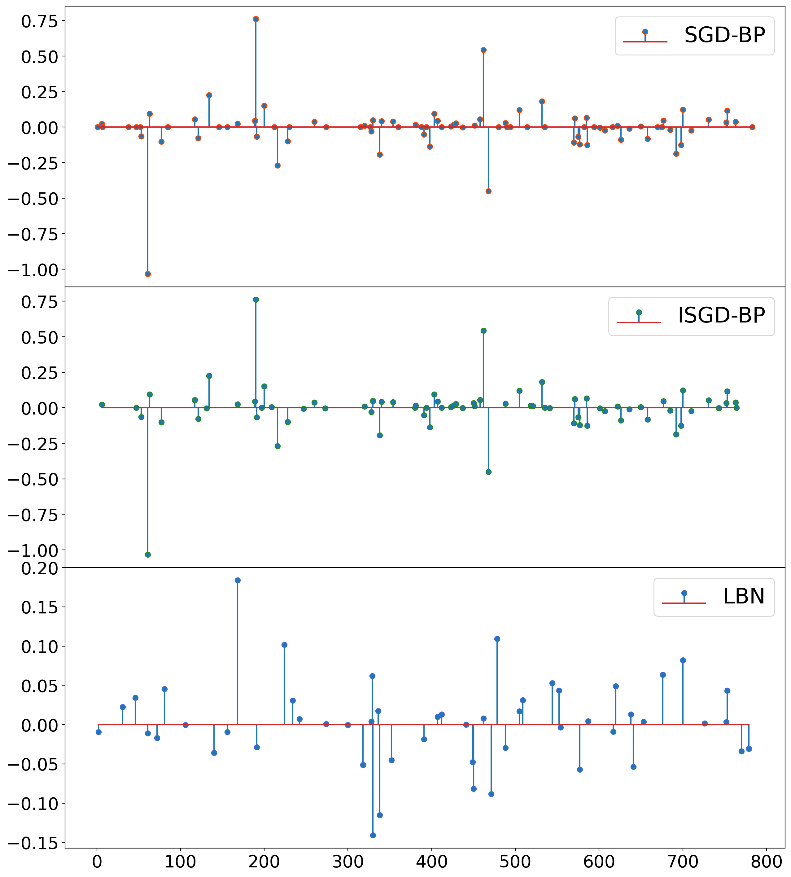
Figure 13: Visualisation of the sparse coding of the sandal image object from Figure 12 computed with the SGD-BP, ISGD-BP, and LBN, respectively. Note that the scaling of the sparse coefficients is slightly different for LBN in comparison to SGD-BP and ISGD-BP.

Appendix C Numerical Results

In the section we provide numerical results in addition to the ones provided in Section 4.

C.1 Visualisations

This section includes additional visualisations of the sparse autoencoder and sparse denoising autoencoder outputs. The compression of the input data is achieved by ensuring that only relatively few coefficients of the code are non-zero. As mentioned earlier, the advantage over conventional autoencoders is that the position of the non-zero coefficients can vary for every input. We also provide visualisations of codes from a sample input image computed with the SGD-BP, ISGD-BP and LBN approach in Figure 13.

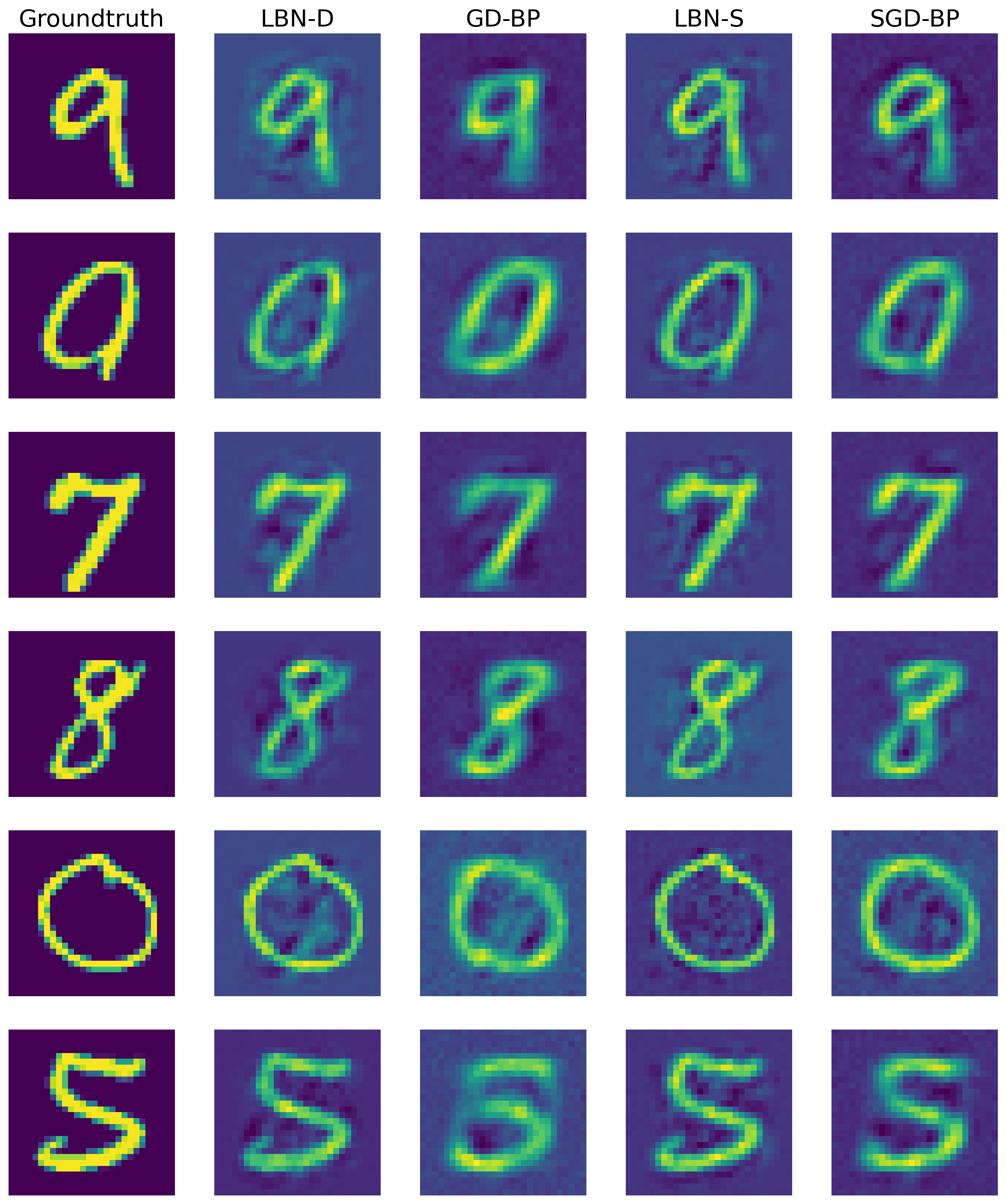
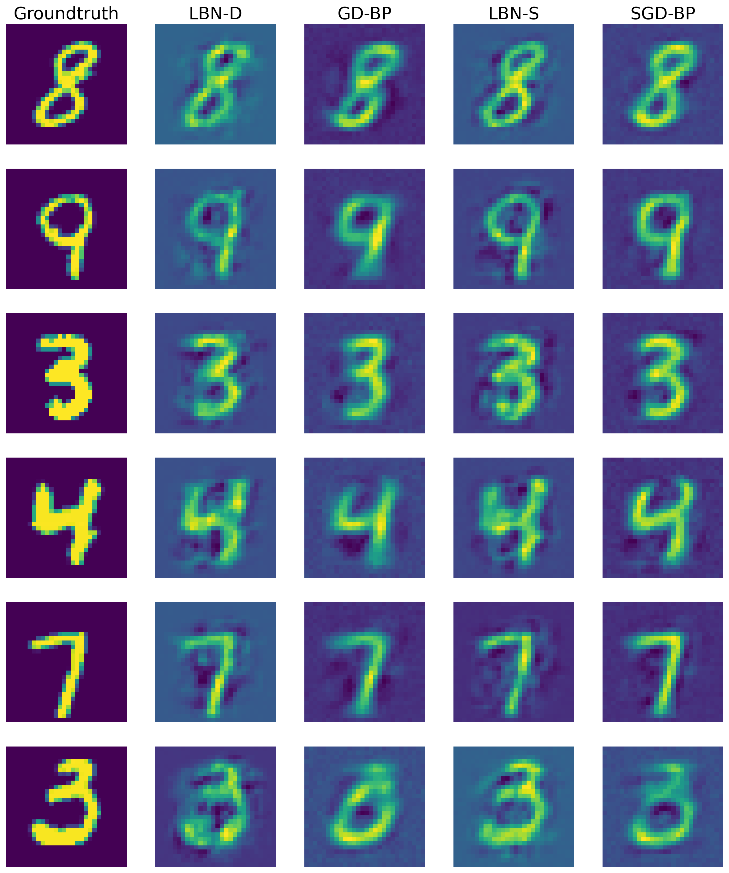
Figure 14: Left:This plot shows selected denoised MNIST training images computed with LBN-D, GD-BP, LBN-S and SGD-BP. Right: This plot shows selected denoising results on the MNIST validation dataset.

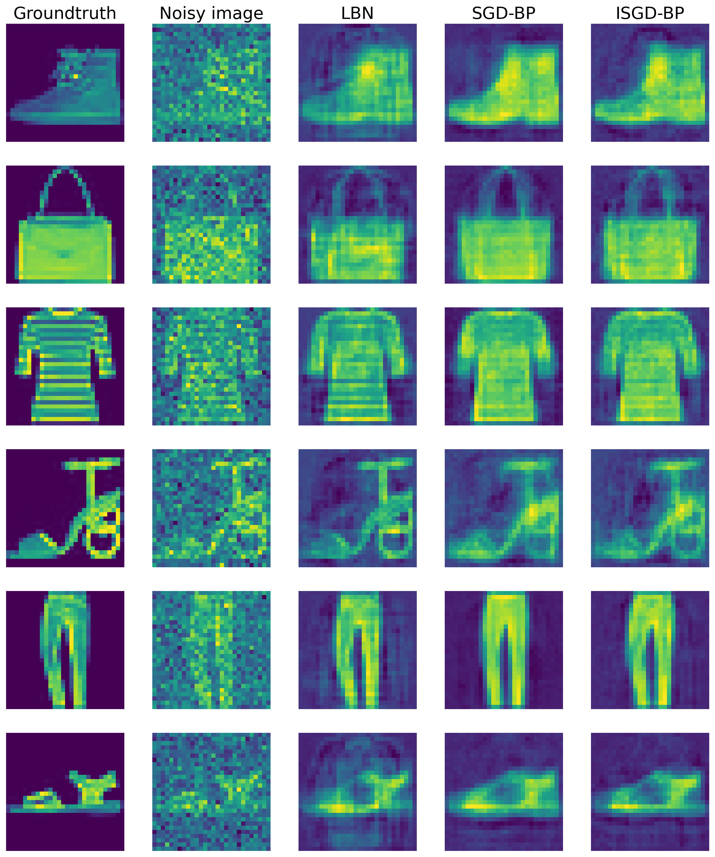
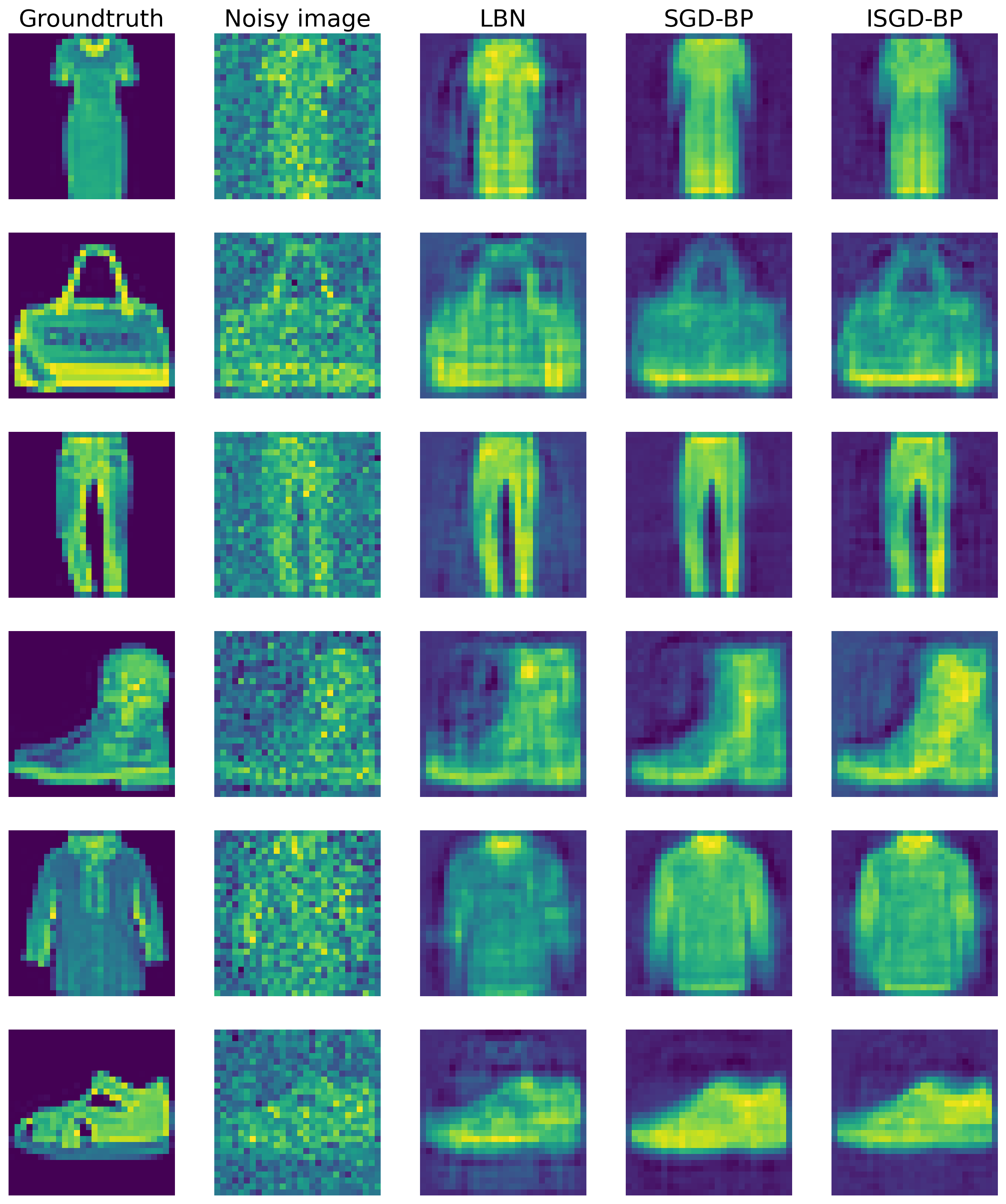
Figure 15: Left: Denoised images from the Fashion-MNIST-1K training dataset computed with LBN, SGD-BP and ISGD-BP for 50 epochs, along with the noise-free and noisy images. Right: Denoised images from the Fashion-MNIST-1K validation dataset computed with LBN, SGD-BP and ISGD-BP for 50 epochs, along with the noise-free and noisy images.

Figure 16: Left: Denoised images from the Fashion-MNIST-10K training dataset computed with LBN, SGD-BP (trained for 1500 epochs) and ISGD-BP, along with the noise-free and noisy images. Right: Denoised images from the Fashion-MNIST-10K validation dataset computed with LBN, SGD-BP (trained for 1500 epochs) and ISGD-BP, along with the noise-free and noisy images.

References

- Alain and Bengio (2014) Guillaume Alain and Yoshua Bengio. What regularized auto-encoders learn from the data-generating distribution. The Journal of Machine Learning Research, 15(1):3563–3593, 2014.
- Askari et al. (2018) Armin Askari, Geoffrey Negiar, Rajiv Sambharya, and Laurent El Ghaoui. Lifted neural networks. arXiv preprint arXiv:1805.01532, 2018.
- Ba et al. (2016) Jimmy Lei Ba, Jamie Ryan Kiros, and Geoffrey E Hinton. Layer normalization. arXiv preprint arXiv:1607.06450, 2016.
- Bauschke et al. (2011) Heinz H Bauschke, Patrick L Combettes, et al. Convex analysis and monotone operator theory in Hilbert spaces, volume 408. Springer, 2011.
- Beck (2017) Amir Beck. First-order methods in optimization. SIAM, 2017.
- Bengio et al. (1994) Yoshua Bengio, Patrice Simard, and Paolo Frasconi. Learning long-term dependencies with gradient descent is difficult. IEEE transactions on neural networks, 5(2):157–166, 1994.
- Bengio et al. (2013) Yoshua Bengio, Aaron Courville, and Pascal Vincent. Representation learning: A review and new perspectives. IEEE transactions on pattern analysis and machine intelligence, 35(8):1798–1828, 2013.
- Benning and Burger (2018) Martin Benning and Martin Burger. Modern regularization methods for inverse problems. Acta Numerica, 27:1–111, 2018.
- Benning and Riis (2021) Martin Benning and Erlend Skaldehaug Riis. Bregman methods for large-scale optimisation with applications in imaging. Handbook of Mathematical Models and Algorithms in Computer Vision and Imaging: Mathematical Imaging and Vision, pages 1–42, 2021.
- Benning et al. (2021) Martin Benning, Marta M Betcke, Matthias J Ehrhardt, and Carola-Bibiane Schönlieb. Choose your path wisely: gradient descent in a bregman distance framework. SIAM Journal on Imaging Sciences, 14(2):814–843, 2021.
- Bolte and Pauwels (2020) Jerome Bolte and Edouard Pauwels. A mathematical model for automatic differentiation in machine learning. Advances in Neural Information Processing Systems, 33:10809–10819, 2020.
- Bregman (1967) Lev M Bregman. The relaxation method of finding the common point of convex sets and its application to the solution of problems in convex programming. USSR computational mathematics and mathematical physics, 7(3):200–217, 1967.
- Bungert et al. (2021) Leon Bungert, Tim Roith, Daniel Tenbrinck, and Martin Burger. A bregman learning framework for sparse neural networks. arXiv preprint arXiv:2105.04319, 2021.
- Burger (2016) Martin Burger. Bregman distances in inverse problems and partial differential equations. In Advances in mathematical modeling, optimization and optimal control, pages 3–33. Springer, 2016.
- Cai et al. (2009) Jian-Feng Cai, Stanley Osher, and Zuowei Shen. Linearized bregman iterations for compressed sensing. Mathematics of computation, 78(267):1515–1536, 2009.
- Candès et al. (2006) Emmanuel J Candès, Justin Romberg, and Terence Tao. Robust uncertainty principles: Exact signal reconstruction from highly incomplete frequency information. IEEE Transactions on information theory, 52(2):489–509, 2006.
- Carreira-Perpinan and Wang (2014) Miguel Carreira-Perpinan and Weiran Wang. Distributed optimization of deeply nested systems. In Artificial Intelligence and Statistics, pages 10–19. PMLR, 2014.
- Censor and Lent (1981) Yair Censor and Arnold Lent. An iterative row-action method for interval convex programming. Journal of Optimization theory and Applications, 34(3):321–353, 1981.
- Censor and Zenios (1992) Yair Censor and Stavros Andrea Zenios. Proximal minimization algorithm with -functions. Journal of Optimization Theory and Applications, 73(3):451–464, 1992.
- Chen and Teboulle (1993) Gong Chen and Marc Teboulle. Convergence analysis of a proximal-like minimization algorithm using bregman functions. SIAM Journal on Optimization, 3(3):538–543, 1993.
- Combettes and Pesquet (2020) Patrick L Combettes and Jean-Christophe Pesquet. Deep neural network structures solving variational inequalities. Set-Valued and Variational Analysis, pages 1–28, 2020.
- De Vito et al. (2005) Ernesto De Vito, Lorenzo Rosasco, Andrea Caponnetto, Umberto De Giovannini, Francesca Odone, and Peter Bartlett. Learning from examples as an inverse problem. Journal of Machine Learning Research, 6(5), 2005.
- De Vito et al. (2021) Ernesto De Vito, Lorenzo Rosasco, and Alessandro Rudi. Regularization: From inverse problems to large-scale machine learning. In Harmonic and Applied Analysis, pages 245–296. Springer, 2021.
- Donoho (2006) David L Donoho. Compressed sensing. IEEE Transactions on information theory, 52(4):1289–1306, 2006.
- Duchi and Singer (2009) John Duchi and Yoram Singer. Efficient online and batch learning using forward backward splitting. The Journal of Machine Learning Research, 10:2899–2934, 2009.
- Eckstein (1993) Jonathan Eckstein. Nonlinear proximal point algorithms using bregman functions, with applications to convex programming. Mathematics of Operations Research, 18(1):202–226, 1993.
- Ekeland and Temam (1999) Ivar Ekeland and Roger Temam. Convex analysis and variational problems. SIAM, 1999.
- Engl et al. (1996) Heinz Werner Engl, Martin Hanke, and Andreas Neubauer. Regularization of inverse problems, volume 375. Springer Science & Business Media, 1996.
- Erhan et al. (2009) Dumitru Erhan, Pierre-Antoine Manzagol, Yoshua Bengio, Samy Bengio, and Pascal Vincent. The difficulty of training deep architectures and the effect of unsupervised pre-training. In Artificial Intelligence and Statistics, pages 153–160. PMLR, 2009.
- Gabay (1983) Daniel Gabay. Applications of the method of multipliers to variational inequalities. In Studies in mathematics and its applications, volume 15, pages 299–331. Elsevier, 1983.
- Geiping and Moeller (2019) Jonas Geiping and Michael Moeller. Parametric majorization for data-driven energy minimization methods. In Proceedings of the IEEE/CVF International Conference on Computer Vision, pages 10262–10273, 2019.
- Glorot and Bengio (2010) Xavier Glorot and Yoshua Bengio. Understanding the difficulty of training deep feedforward neural networks. In Proceedings of the thirteenth international conference on artificial intelligence and statistics, pages 249–256. JMLR Workshop and Conference Proceedings, 2010.
- Goodfellow et al. (2016) Ian Goodfellow, Yoshua Bengio, and Aaron Courville. Deep Learning. MIT Press, 2016. http://www.deeplearningbook.org.
- Gu et al. (2020) Fangda Gu, Armin Askari, and Laurent El Ghaoui. Fenchel lifted networks: A lagrange relaxation of neural network training. In International Conference on Artificial Intelligence and Statistics, pages 3362–3371. PMLR, 2020.
- Hasannasab et al. (2020) Marzieh Hasannasab, Johannes Hertrich, Sebastian Neumayer, Gerlind Plonka, Simon Setzer, and Gabriele Steidl. Parseval proximal neural networks. Journal of Fourier Analysis and Applications, 26(4):1–31, 2020.
- He et al. (2016) Kaiming He, Xiangyu Zhang, Shaoqing Ren, and Jian Sun. Deep residual learning for image recognition. In Proceedings of the IEEE conference on computer vision and pattern recognition, pages 770–778, 2016.
- Higham and Higham (2019) Catherine F Higham and Desmond J Higham. Deep learning: An introduction for applied mathematicians. Siam review, 61(4):860–891, 2019.
- Hinton et al. (2012) Geoffrey E Hinton, Nitish Srivastava, Alex Krizhevsky, Ilya Sutskever, and Ruslan R Salakhutdinov. Improving neural networks by preventing co-adaptation of feature detectors. arXiv preprint arXiv:1207.0580, 2012.
- Høier and Zach (2020) Rasmus Kjær Høier and Christopher Zach. Lifted regression/reconstruction networks. arXiv preprint arXiv:2005.03452, 2020.
- Huang et al. (2013) Bo Huang, Shiqian Ma, and Donald Goldfarb. Accelerated linearized bregman method. Journal of Scientific Computing, 54(2):428–453, 2013.
- Ioffe and Szegedy (2015) Sergey Ioffe and Christian Szegedy. Batch normalization: Accelerating deep network training by reducing internal covariate shift. In International conference on machine learning, pages 448–456. PMLR, 2015.
- Kiefer and Wolfowitz (1952) Jack Kiefer and Jacob Wolfowitz. Stochastic estimation of the maximum of a regression function. The Annals of Mathematical Statistics, pages 462–466, 1952.
- Kiwiel (1997) Krzysztof C Kiwiel. Proximal minimization methods with generalized bregman functions. SIAM journal on control and optimization, 35(4):1142–1168, 1997.
- LeCun et al. (1988) Yann LeCun, D Touresky, G Hinton, and T Sejnowski. A theoretical framework for back-propagation. In Proceedings of the 1988 connectionist models summer school, volume 1, pages 21–28, 1988.
- LeCun et al. (1998) Yann LeCun, Léon Bottou, Yoshua Bengio, and Patrick Haffner. Gradient-based learning applied to document recognition. Proceedings of the IEEE, 86(11):2278–2324, 1998.
- Li et al. (2019) Jia Li, Cong Fang, and Zhouchen Lin. Lifted proximal operator machines. In Proceedings of the AAAI Conference on Artificial Intelligence, volume 33 No. 01., 2019.
- Lions and Mercier (1979) Pierre-Louis Lions and Bertrand Mercier. Splitting algorithms for the sum of two nonlinear operators. SIAM Journal on Numerical Analysis, 16(6):964–979, 1979.
- McDonald et al. (2010) Ryan McDonald, Keith Hall, and Gideon Mann. Distributed training strategies for the structured perceptron. In Human language technologies: The 2010 annual conference of the North American chapter of the association for computational linguistics, pages 456–464, 2010.
- Moreau (1962) Jean Jacques Moreau. Fonctions convexes duales et points proximaux dans un espace hilbertien. Comptes rendus hebdomadaires des séances de l’Académie des sciences, 255:2897–2899, 1962.
- Moreau (1965) Jean-Jacques Moreau. Proximité et dualité dans un espace hilbertien. Bulletin de la Société mathématique de France, 93:273–299, 1965.
- Mukkamala et al. (2020) Mahesh Chandra Mukkamala, Peter Ochs, Thomas Pock, and Shoham Sabach. Convex-concave backtracking for inertial bregman proximal gradient algorithms in nonconvex optimization. SIAM Journal on Mathematics of Data Science, 2(3):658–682, 2020.
- Nair and Hinton (2010) Vinod Nair and Geoffrey E Hinton. Rectified linear units improve restricted boltzmann machines. In Icml, 2010.
- Nemirovski et al. (2009) Arkadi Nemirovski, Anatoli Juditsky, Guanghui Lan, and Alexander Shapiro. Robust stochastic approximation approach to stochastic programming. SIAM Journal on optimization, 19(4):1574–1609, 2009.
- Nesterov (1983) Yurii E Nesterov. A method for solving the convex programming problem with convergence rate . In Dokl. akad. nauk Sssr, volume 269, pages 543–547, 1983.
- Ng et al. (2011) Andrew Ng et al. Sparse autoencoder. CS294A Lecture notes, 72(2011):1–19, 2011.
- Osher et al. (2005) Stanley Osher, Martin Burger, Donald Goldfarb, Jinjun Xu, and Wotao Yin. An iterative regularization method for total variation-based image restoration. Multiscale Modeling & Simulation, 4(2):460–489, 2005.
- Robbins and Monro (1951) Herbert Robbins and Sutton Monro. A stochastic approximation method. The annals of mathematical statistics, pages 400–407, 1951.
- Rockafellar (1970) R Tyrrell Rockafellar. Convex Analysis, volume 36. Princeton University Press, 1970.
- Rosasco et al. (2019) Lorenzo Rosasco, Silvia Villa, and Bang Công Vũ. Convergence of stochastic proximal gradient algorithm. Applied Mathematics & Optimization, pages 1–27, 2019.
- Rumelhart et al. (1986) David E Rumelhart, Geoffrey E Hinton, and Ronald J Williams. Learning representations by back-propagating errors. nature, 323(6088):533–536, 1986.
- Stuart (2010) Andrew M Stuart. Inverse problems: a bayesian perspective. Acta numerica, 19:451–559, 2010.
- Taylor et al. (2016) Gavin Taylor, Ryan Burmeister, Zheng Xu, Bharat Singh, Ankit Patel, and Tom Goldstein. Training neural networks without gradients: A scalable admm approach. In International conference on machine learning, pages 2722–2731. PMLR, 2016.
- Teboulle (1992) Marc Teboulle. Entropic proximal mappings with applications to nonlinear programming. Mathematics of Operations Research, 17(3):670–690, 1992.
- Teboulle (2018) Marc Teboulle. A simplified view of first order methods for optimization. Mathematical Programming, 170(1):67–96, 2018.
- Toulis and Airoldi (2017) Panos Toulis and Edoardo M Airoldi. Asymptotic and finite-sample properties of estimators based on stochastic gradients. The Annals of Statistics, 45(4):1694–1727, 2017.
- Vaswani et al. (2017) Ashish Vaswani, Noam Shazeer, Niki Parmar, Jakob Uszkoreit, Llion Jones, Aidan N Gomez, Łukasz Kaiser, and Illia Polosukhin. Attention is all you need. Advances in neural information processing systems, 30, 2017.
- Wang and Benning (2020) Xiaoyu Wang and Martin Benning. Generalised perceptron learning. 12th OPT Workshop on Optimization for Machine Learning at 34th Conference on Neural Information Processing Systems (NeurIPS), 2020.
- Xiao et al. (2017) Han Xiao, Kashif Rasul, and Roland Vollgraf. Fashion-mnist: a novel image dataset for benchmarking machine learning algorithms. arXiv preprint arXiv:1708.07747, 2017.
- Xie et al. (2012) Junyuan Xie, Linli Xu, and Enhong Chen. Image denoising and inpainting with deep neural networks. Advances in neural information processing systems, 25, 2012.
- Yosida (1964) Kösaku Yosida. Functional analysis. Springer, 1964.
- Zach and Estellers (2019) Christopher Zach and Virginia Estellers. Contrastive learning for lifted networks. British Machine Vision Conference (BMVC), 2019. URL https://bmvc2019.org/wp-content/uploads/papers/0830-paper.pdf.
- Zhang et al. (2021) Chiyuan Zhang, Samy Bengio, Moritz Hardt, Benjamin Recht, and Oriol Vinyals. Understanding deep learning (still) requires rethinking generalization. Communications of the ACM, 64(3):107–115, 2021.
- Zhang and Brand (2017) Ziming Zhang and Matthew Brand. On the convergence of block coordinate descent in training dnns with tikhonov regularization. In Advances in Neural Information Processing Systems, pages 1719–1728, 2017.
- Zinkevich et al. (2010) Martin Zinkevich, Markus Weimer, Lihong Li, and Alex Smola. Parallelized stochastic gradient descent. Advances in neural information processing systems, 23, 2010.