Quantum phase detection generalization from marginal quantum neural network models
![[Uncaptioned image]](/html/2208.08748/assets/ORCIDiD_icon128x128.png) Oriel Kiss
Antonio Mandarino
Sofia Vallecorsa
Michele Grossi
Oriel Kiss
Antonio Mandarino
Sofia Vallecorsa
Michele Grossi
Zusammenfassung
Quantum machine learning offers a promising advantage in extracting information about quantum states, e.g. phase diagram. However, access to training labels is a major bottleneck for any supervised approach, preventing getting insights about new physics. In this Letter, using quantum convolutional neural networks, we overcome this limit by determining the phase diagram of a model where analytical solutions are lacking, by training only on marginal points of the phase diagram, where integrable models are represented. More specifically, we consider the axial next-nearest-neighbor Ising (ANNNI) Hamiltonian, which possesses a ferromagnetic, paramagnetic and antiphase, showing that the whole phase diagram can be reproduced.
Introduction. Quantum machine learning (QML) Biamonte et al. (2017), where parametrized quantum circuits Benedetti et al. (2019) act as statistical models, has attracted much attention recently, with applications to natural sciences Kiss et al. (2022a); Ngairangbam et al. (2022); Zhou et al. (2021); Wu et al. (2021); Li et al. (2020); Mitarai et al. (2018) or in generative modeling Brian Coyle et al. (2020); Zoufal et al. (2019); Rudolph et al. (2022); Kiss et al. (2022b); Delgado and Hamilton (2022). Even if QML models benefit from high expressivity Abbas et al. (2021) and demonstrated superiority over classical models in some specific cases Huang et al. (2021); Glick et al. (2021), it is still unclear what kind of advantage could be obtained with quantum computers Schuld and Killoran (2022) in the era of deep neural networks.
Quantum data, on the other hand, could be a natural paradigm to apply QML, where quantum advantages have already been demonstrated Huang et al. (2022a). There is hope that quantum data could be collected via quantum sensors Marciniak et al. (2022), and eventually directly linked to quantum computers. In this Letter, we emulate the possibility of working with quantum data by constructing them directly on a quantum device. We use a variational ground state solver to obtain approximations of the true ground states in order to mimic noisy real world data. Specifically, this Letter addresses the computation of the phase diagram of the ground states of a Hamiltonian using a supervised learning approach. Even if similar problems have already been explored for the binary case Cong et al. (2019); Uvarov et al. (2020a), with multiple classes Lazzarin et al. (2022) and computed on a superconducting platform Herrmann et al. (2022), all of these approaches suffer from a limitation by construction, a bottleneck. In fact, since labels are needed for the training, and because they are computed analytically or numerically, these techniques can only speed up calculations, but cannot extend beyond their validated domain. Alternatively, anomaly detection (AD), an unsupervised learning technique, has been proposed Kottmann et al. (2020, 2021) as a way to bypass this bottleneck, by finding structure inside the data set. However, AD can only obtain qualitative, possibly unstable, results and the performance can therefore be difficult to assess. Instead, the proposed approach provides a clear prediction for the boundaries of the adopted model, with the possibility to evaluate the performance on a validation set.
This Letter numerically demonstrates that QML can make predictions to regions where analytical labels do not exist, after being only trained on easily computable subregions. Moreover, QML only needs very few training labels to do so, as already pointed out by Caro et al. (2022a); Banchi et al. (2021). In particular, we make a step toward an out-of-distribution generalization Caro et al. (2022b), where the training and testing set do not belong to the same data distribution, which is known to be a difficult task Ye et al. (2021). This drastically changes the perspective, extending QML capabilities to extrapolate and eventually discover new physics when trained on well-established simpler models.
The model. We consider the axial next-nearest-neighbour Ising (ANNNI) model
| (1) |
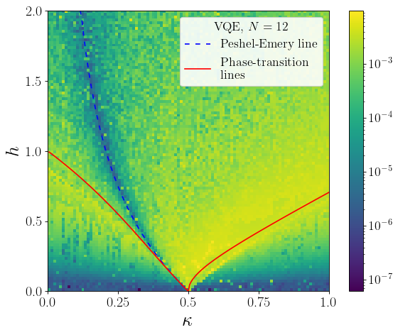
where are the Pauli matrices acting on the th spin, and we assume open boundary conditions. The energy scale of the Hamiltonian is given by the coupling constant (without loss of generality we set ), while the dimensionless parameters and account for the next-nearest-neighbor interaction and the transverse magnetic field, respectively. We restrict ourselves to , and even . The difference of sign between the nearest and next-nearest interactions, leading to a ferro- or antiferro-magnetic exchange in the system, is responsible for the magnetic frustration. Thence, the ANNNI model offers the possibility to study the competing mechanism of quantum fluctuations due to the transverse magnetic field and frustration. The phase diagram of the quantum model at K temperature has been studied mainly by renormalization group or Monte Carlo techniques in dimensions exploiting also the correspondence with the classical analog in dimensions Selke (1988); Guimarães et al. (2002); Chandra and Dasgupta (2007); Beccaria et al. (2006, 2007); Canabarro et al. (2019). The phase diagram is quite rich and three phases have been confirmed, separated by two second-order phase transitions. The first, for low frustration of the Ising type separates the ferromagnetic and the paramagnetic phases along the line . The other one of a commensurate-incommensurate type appears between the paramagnetic phase and an antiphase for values of the field , in the high frustration sector . As usual, the paramagnetic phase is the disordered one, in contrast with the two ordered phases: the ferromagnetic and the antiphase one. In particular, they are different because the former is characterized by all the spins aligned along the field direction, and the latter has a four-spin periodicity, composed of repetitions of two pairs of spins pointing in opposite directions. The point represents a multicritical point.
We mention here that other relevant lines have been numerically addressed but not confirmed. One signaling an infinite-order phase transition of the Berezinskii–Kosterlitz–Thouless (BKT) type for delimiting a floating phase between the paramagnetic and the antiphase Beccaria et al. (2007), and a disorder line where the model is exactly solvable known as the Peschel-Emery (PE) line Peschel and Emery (1981); Beccaria et al. (2006).
Variational state preparation.
The purpose of the variational quantum eigensolver (VQE) Peruzzo et al. (2014) is to calculate the ground state energy
of a Hamiltonian on a quantum computer. Using the Rayleigh-Ritz variational principle, the VQE minimizes the energy expectation value of a parametrized wavefunction and has been successfully applied in quantum chemistry Kandala et al. (2017); Barkoutsos et al. (2018); Romero et al. (2019), in nuclear physics Dumitrescu et al. (2018); Stetcu et al. (2022); Kiss et al. (2022c) or in frustrated magnetic systems Uvarov et al. (2020b); Grossi et al. (2022).
Here, we are interested in the final eigenstates, represented by an ansatz , to be used as quantum data.
Typically, the ansatz is chosen as a hardware-efficient (HEA) quantum circuit Kandala et al. (2017); Sim et al. (2019), which is built with low connectivity and gates that can be easily run on noisy intermediate-scale quantum (NISQ) Preskill (2018) devices. For instance, we use repetitions of a layer consisting of free rotations around the axis and controlled-NOT (CNOT) gates with linear connectivity CXi,i+1 for Nielsen and Chuang (2010), for spin systems. The optimization is performed using the gradient-descent-based ADAM algorithm Kingma and Ba (2015), with an initial learning rate of 0.3 and a parameter recycling scheme to improve the convergence Harwood et al. (2022). Moreover, we note that the VQE can also be used to recursively compute excited states Higgott et al. (2019), which we used to show that the ground states of the ANNNI model are only degenerate at the boundaries in the phase diagram, where the ground states corresponding to the different phases are competing, excluding the bit flip symmetry at . Finally, we asses the accuracy of the VQE states by comparing with the exact energy and observe that the relative error ratio is always below 1%. Moreover, it seems that the energy accuracy distribution is able to reveal the Peschel-Emery line, since the predicted energy values are more accurate along it. More details about the implementation, optimization, degeneracy and accuracy can be found in Appendix A.
Quantum convolutional neural networks (QCNNs).
QCNNs are a class of quantum circuits, inspired by classical convolutional neural networks (CNN) LeCun et al. (1989), originally proposed in Cong et al. (2019). The QCNN is trained to detect quantum phase transitions, effectively learning an observable that linearly separates two states and from two different phases and , such that Huang et al. (2022b), which exist since the phases in the ANNNI model are not topological. Intuitively, non topological phases of matter exhibit macroscopic differences, which can be captured by the variational observable . In principle, quantum phase detection could be performed by measuring different string order parameters (SOPs) Cong et al. (2019). However, the SOP vanishes near the phase transition, thus requiring exponentially many samples for the classification. On the other hand, the QCNN output is much sharper, therefore reducing the sample complexity. This changes quantum phase detection to the task of designing and training an appropriate ansatz.
In our implementation, the QCNN starts with a free rotation layer around the axis, followed by blocks consisting of convolutions, free rotations, and pooling layers that halve the number of qubits to until , where it the total number of quantum phases. Finally, a fully connected layer and measurement are performed in the computational basis.
An example with qubits is shown in Figure 1 where we have free axis rotations (yellow), , two-qubit convolutions (light green) , pooling (red) with the value of the measured qubit, and a two-qubit fully connected (dark green) gate .
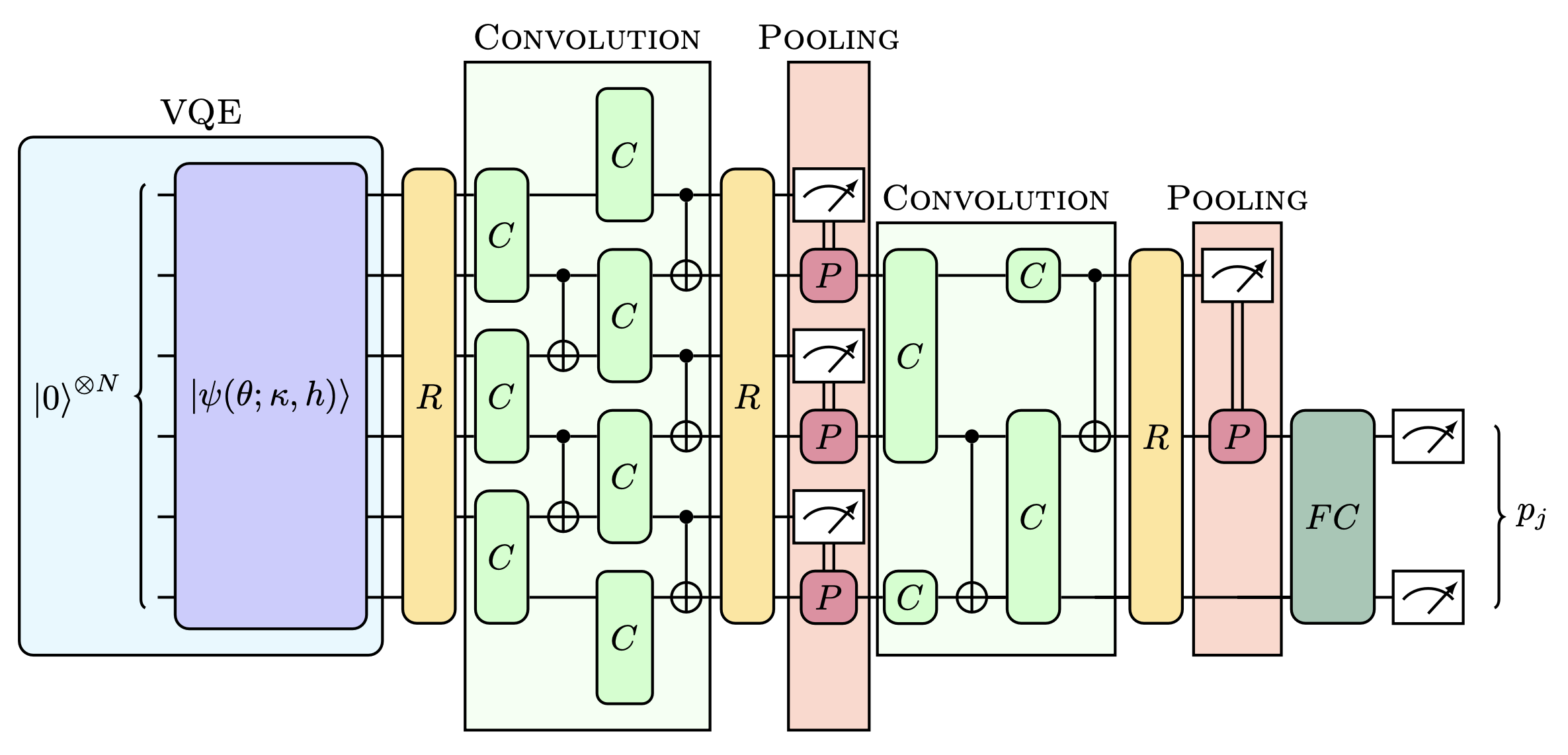
QCNNs have been shown to be resistant to barren plateaus Pesah et al. (2021) due to their distance from low design and are therefore good candidates for any quantum learning tasks. The analogy with CNN holds in the quantum settings since convolution and pooling layers are functions of shared parameters and the reduction of the circuit’s dimension is guaranteed by the intermediate measurement. The whole algorithm flow starts with the QCNN taking as input ground states from the Hamiltonian family , obtained through the VQE. The quantum network then outputs the probability ) of being in one of the phases (ferromagnetic, paramagnetic or antiphase), where is computed as the probability of measuring the state on the two output qubits. Since the phase diagram of the ANNNI model only contains three phases, the state is interpreted as a garbage class.
Generalization.
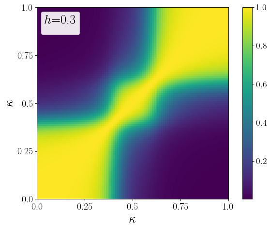
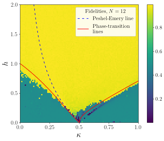
The main contribution of this Letter is to demonstrate the ability of QCNN to work in a partial supervised approach and thus get closer to an out-of-distribution generalization by training on a set of easily available labels. We first argue that this generalization is expected to hold according to Banchi et al. (2021) if the ground states of the ANNNI model are clustered, i.e., if the fidelity between states in the same phase is high Bina et al. (2014); Mandarino et al. (2014, 2016), while being low between different phases. This is indeed the case as shown in Figure 2 along the line for the spin case.
Even if the requirements of the generalisation results from Caro et al. (2022a) do not hold since the training data are only located on the boundaries, and specifically not independent and identically distributed (i.i.d.), we observe a numerical agreement with the generalization error’s scaling behavior predicted in Ref. Caro et al. (2022a), i.e., , where is the number of parameters and the number of training points. Since the QCNN is composed of parameters Cong et al. (2019), we can control the expected risk by training on points.
Training set. The training data set consists of the composition of points from two analytical models derived from the simplification of the physical model used. Specifically, we consider the integrable Ising model in transverse field in the case and the quasi classical model when , where quantum fluctuations no longer exist. We demonstrate that QCNNs extend their prediction to the all phase diagram when only trained on the marginal model given by . We consider three types of subsets , where training points are sampled normally around each critical point {(0,1), (0.5,0)}, where training points are sampled normally at the middle of each phase {(0,1.5), (0,0.5), (0.25,0), (0.75,0)} and where data points are drawn uniformly on both axes. The QCNN is trained using the cross entropy loss,
| (2) |
between the one-hot classical labels and the predictions on the training region of the phase space.
Results.
Once we have introduced the problem and defined the techniques used, we can analyze the quality of the results obtained under ideal conditions with a quantum simulator.
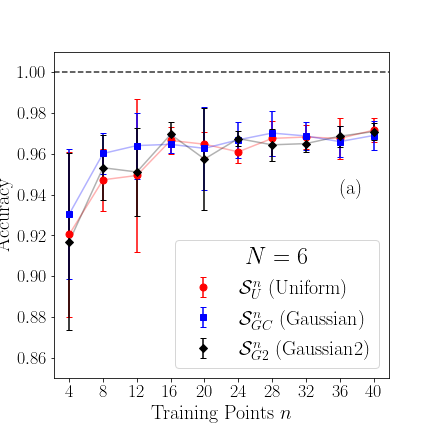
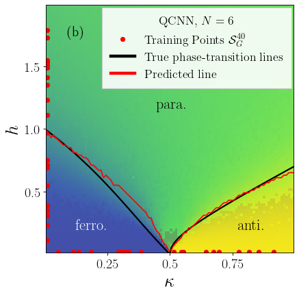
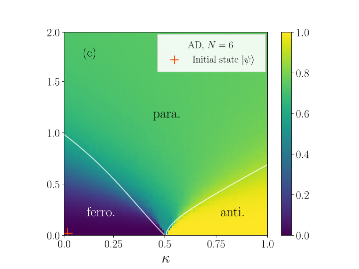
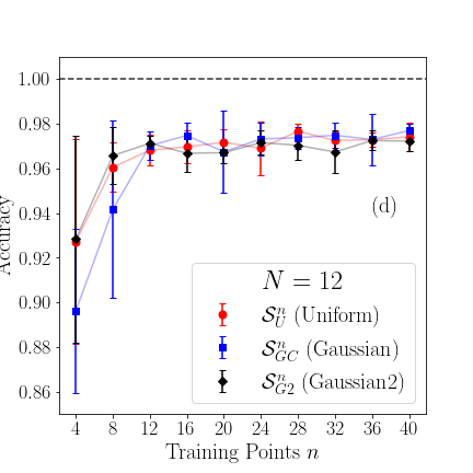
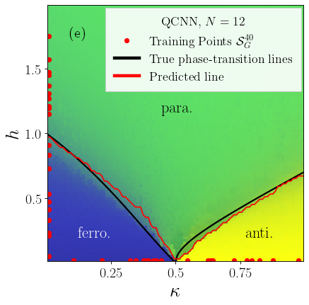
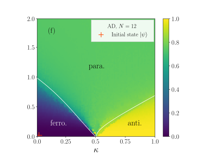
We study our ability to reconstruct the phase diagram of the ANNNI model, characterized by a non trivial disordered paramagnetic phase, the ordered ferromagnetic phase, and antiphase one. To test the stability of the proposed approach, we consider the model with an increasing number of spins and sampling a different number of points used for the training. By virtue of the quality of the results, we evaluated the influence of different sampling of the training points corresponding to the two physical models that could affect the quality of the classification. A summary of the results can be qualitatively seen in Figure 3, while more quantitative results for the QCNN are displayed in Appendix B. In the first row, we have the phase diagram reconstruction for the ANNNI model with six spins, where the black lines represent the analytical transition explained above in the model section. The second line in the figure shows the same for a system with spins.
The first column shows the accuracy, computed on the whole phase space, as a function of the number of training points , for the Gaussian centered around the critical points (blue), around the middle of each phase (black), and the uniform (red) sampling scheme, where the error bars correspond to one standard deviation from ten independent runs. We observe that the accuracy quickly increases with , before saturating for , as argued in Ref. Caro et al. (2022a) and that the sampling strategy does not play a major role. More importantly, sampling away from the critical points is enough. The second column displays the phase diagram obtained with the QCNN trained on points. Colour shades represent the continuous probability distribution of the QCNN for our multiclass classifier as a probability mixture (blue, green and yellow times the relevant probability), while the red lines represent the predicted boundaries. The individual probabilities of each phases predicted by the QCNN are shown in Appendix B. The last column instead shows the comparison to the unsupervised learning approach inspired from Kottmann et al. (2021) where the autoencoder is trained to compress the single red cross , and tested on the remaining points. In a nutshell, the autoencoder is expected to perform poorly if the states are far away in the Hilbert space, i.e., if they belong to different phases, thus leading to a high compression score. The color scale shows the compression loss of each state. Additional details about the implementation of the anomaly detection can be found in Appendix C. It is worth noting that although only one training point is sufficient to obtain a qualitatively good phase diagram, only QCNNs allow a quantitative prediction for the phase. Moreover, while the QCNNs are stable when changing the training set, it is easy to find initial states where AD performs poorly, for instance by starting in the paramagnetic phase. The relatively good performance of AD can be explained by the product state nature of the training point. Hence, the product state can be easily compressed with the autoencoder Romero et al. (2017), while states corresponding to a high magnetic field cannot.
Conclusions.
This Letter addresses the computation of the phase diagram of a non integrable model, by training a QCNN on the limiting integrable regions of the considered ANNNI model. We provide numerical evidence that the QCNNs are able to generalize from non-i.i.d. training data, which is a challenging task in general. The numerical simulations suggest that QCNNs can carry this task with more than accuracy, using only quantum data points distributed on the two integrable axes of the phase space. Moreover, the data points do not need to be close to the critical points. The accuracy of the QCNN quickly increases to reach its maximum as a function of the number of training points, suggesting that QCNNs can generalize from a few data points. Being a supervised method, the QCNN is not able to detect phases that are not present in the training set , i.e., the boundaries, such as the BKT phase transition and the PE line. Nevertheless, AD is also not able to reveal them and is limited to qualitative predictions, while a supervised approach gives quantitative results whose quality can be easily evaluated on the validation set. Moreover, by approaching out-of-distribution generalization, we propose a solution to the bottleneck of needing training labels, that are generally challenging to obtain. Consequently, we make a step into extending the reach of QML to useful applications in physics. Future work should be performed to detect phases not present in the training set, such as the floating phase or the PE line, by either affording training points inside these unrepresented phases or mixing the QCNN with the unsupervised approach.
Acknowledgments
The authors would like to thank Zoë Holmes for useful discussions about generalization. S.M., O.K., and M.G. are supported by CERN through the CERN Quantum Technology Initiative. A.M. is supported by Foundation for Polish Science (FNP), IRAP project ICTQT, contract No. 2018/MAB/5, co financed by EU Smart Growth Operational Program, and (Polish) National Science Center (NCN), MINIATURA DEC-2020/04/X/ST2/01794.
Code Availability
The code used to generate the data set and the figures of the present Letter is publicly available sof .
Literatur
- Biamonte et al. (2017) Jacob Biamonte, Peter Wittek, Nicola Pancotti, Patrick Rebentrost, Nathan Wiebe, and Seth Lloyd, “Quantum machine learning,” Nature 549, 195–202 (2017).
- Benedetti et al. (2019) Marcello Benedetti, Erika Lloyd, Stefan Sack, and Mattia Fiorentini, “Parameterized quantum circuits as machine learning models,” Quantum Science and Technology 4, 4 (2019).
- Kiss et al. (2022a) Oriel Kiss, Francesco Tacchino, Sofia Vallecorsa, and Ivano Tavernelli, “Quantum neural networks force field generation,” Mach. Learn.: Sci. Technol. 3 (2022a), https://doi.org/10.1088/2632-2153/ac7d3c.
- Ngairangbam et al. (2022) Vishal S. Ngairangbam, Michael Spannowsky, and Michihisa Takeuchi, “Anomaly detection in high-energy physics using a quantum autoencoder,” Phys. Rev. D 105, 095004 (2022).
- Zhou et al. (2021) Chen Zhou, Jay Chan, Wen Guan, Shaojun Sun, Alex Zeng Wang, Sau Lan Wu, Miron Livny, Federico Carminati, Alberto Di Meglio, Andy C. Y. Li, Joseph Lykken, Panagiotis Spentzouris, Samuel Yen-Chi Chen, Shinjae Yoo, and Tzu-Chieh Wei, “Application of Quantum Machine Learning to High Energy Physics Analysis at LHC using IBM Quantum Computer Simulators and IBM Quantum Computer Hardware,” PoS ICHEP2020, 930 (2021).
- Wu et al. (2021) Sau Lan Wu, Jay Chan, Wen Guan, Shaojun Sun, Alex Wang, Chen Zhou, Miron Livny, Federico Carminati, Alberto Di Meglio, Andy C Y Li, Joseph Lykken, Panagiotis Spentzouris, Samuel Yen-Chi Chen, Shinjae Yoo, and Tzu-Chieh Wei, “Application of quantum machine learning using the quantum variational classifier method to high energy physics analysis at the LHC on IBM quantum computer simulator and hardware with 10 qubits,” Journal of Physics G: Nuclear and Particle Physics 48, 125003 (2021).
- Li et al. (2020) YaoChong Li, Ri-Gui Zhou, RuQing Xu, Jia Luo, and WenWen Hu, “A quantum deep convolutional neural network for image recognition,” Quantum Science and Technology 5, 044003 (2020).
- Mitarai et al. (2018) K. Mitarai, M. Negoro, M. Kitagawa, and K. Fujii, “Quantum circuit learning,” Phys. Rev. A 98, 032309 (2018).
- Brian Coyle et al. (2020) Daniel Mills Brian Coyle, Vincent Danos, and Elham Kashefi, “The born supremacy: quantum advantage and training of an ising born machine,” npj Quantum Inf 6, 60 (2020).
- Zoufal et al. (2019) Christa Zoufal, Aurélien Lucchi, and Stefan Woerner, “Quantum generative adversarial networks for learning and loading random distributions,” npj Quantum Inf 5 (2019), https://doi.org/10.1038/s41534-019-0223-2.
- Rudolph et al. (2022) Manuel S. Rudolph, Ntwali Bashige Toussaint, Amara Katabarwa, Sonika Johri, Borja Peropadre, and Alejandro Perdomo-Ortiz, “Generation of high-resolution handwritten digits with an ion-trap quantum computer,” Phys. Rev. X 12, 031010 (2022).
- Kiss et al. (2022b) Oriel Kiss, Michele Grossi, Enrique Kajomovitz, and Sofia Vallecorsa, “Conditional born machine for monte carlo event generation,” Phys. Rev. A 106, 022612 (2022b).
- Delgado and Hamilton (2022) Andrea Delgado and Kathleen E. Hamilton, “Unsupervised quantum circuit learning in high energy physics,” Phys. Rev. D 106, 096006 (2022).
- Abbas et al. (2021) Amira Abbas, David Sutter, Christa Zoufal, Aurelien Lucchi, Alessio Figalli, and Stefan Woerner, “The power of quantum neural networks,” Nature Computational Science 1, 403–409 (2021).
- Huang et al. (2021) Hsin-Yuan Huang, Michael Broughton, Masoud Mohseni, Ryan Babbush, Sergio Boixo, Hartmut Neven, and Jarrod R. McClean, “Power of data in quantum machine learning,” Nat Commun 2631 (2021), https://doi.org/10.1038/s41467-021-22539-9.
- Glick et al. (2021) Jennifer R. Glick, Tanvi P. Gujarati, Antonio D. Corcoles, Youngseok Kim, Abhinav Kandala, Jay M. Gambetta, and Kristan Temme, “Covariant quantum kernels for data with group structure,” ArXiv e-prints (2021), arXiv:2105.03406 [quant-ph] .
- Schuld and Killoran (2022) Maria Schuld and Nathan Killoran, “Is quantum advantage the right goal for quantum machine learning?” PRX Quantum 3, 030101 (2022).
- Huang et al. (2022a) Hsin-Yuan Huang, Michael Broughton, Jordan Cotler, Sitan Chen, Jerry Li, Masoud Mohseni, Hartmut Neven, Ryan Babbush, Richard Kueng, John Preskill, and Jarrod R. McClean, “Quantum advantage in learning from experiments,” Science 376, 1182–1186 (2022a).
- Marciniak et al. (2022) Christian D. Marciniak, Thomas Feldker, Ivan Pogorelov, Raphael Kaubruegger, Denis V. Vasilyev, Rick van Bijnen, Philipp Schindler, Peter Zoller, Rainer Blatt, and Thomas Monz, “Optimal metrology with programmable quantum sensors,” Nature 603, 604–609 (2022).
- Cong et al. (2019) Iris Cong, Soonwon Choi, and Mikhail D. Lukin, “Quantum convolutional neural networks,” Nat. Phys. 15, 1273–1278 (2019).
- Uvarov et al. (2020a) A. V. Uvarov, A. S. Kardashin, and J. D. Biamonte, “Machine learning phase transitions with a quantum processor,” Phys. Rev. A 102, 012415 (2020a).
- Lazzarin et al. (2022) Marco Lazzarin, Davide Emilio Galli, and Enrico Prati, “Multi-class quantum classifiers with tensor network circuits for quantum phase recognition,” Physics Letters A 434, 128056 (2022).
- Herrmann et al. (2022) Johannes Herrmann, Sergi Masot Llima, Ants Remm, Petr Zapletal, Nathan A. McMahon, Colin Scarato, François Swiadek, Christian Kraglund Andersen, Christoph Hellings, Sebastian Krinner, Nathan Lacroix, Stefania Lazar, Michael Kerschbaum, Dante Colao Zanuz, Graham J. Norris, Michael J. Hartmann, Andreas Wallraff, and Christopher Eichler, “Realizing quantum convolutional neural networks on a superconducting quantum processor to recognize quantum phases,” Nat Commun 13 (2022), https://doi.org/10.1038/s41467-022-31679-5.
- Kottmann et al. (2020) Korbinian Kottmann, Patrick Huembeli, Maciej Lewenstein, and Antonio Acín, “Unsupervised phase discovery with deep anomaly detection,” Phys. Rev. Lett. 125, 170603 (2020).
- Kottmann et al. (2021) Korbinian Kottmann, Friederike Metz, Joana Fraxanet, and Niccolò Baldelli, “Variational quantum anomaly detection: Unsupervised mapping of phase diagrams on a physical quantum computer,” Phys. Rev. Research 3, 043184 (2021).
- Caro et al. (2022a) Matthias C. Caro, Hsin-Yuan Huang, M. Cerezo, Kunal Sharma, Andrew Sornborger, Lukasz Cincio, and Patrick J. Coles, “Generalization in quantum machine learning from few training data,” Nat Commun 13, 4919 (2022a).
- Banchi et al. (2021) Leonardo Banchi, Jason Pereira, and Stefano Pirandola, “Generalization in quantum machine learning: A quantum information standpoint,” PRX Quantum 2, 040321 (2021).
- Caro et al. (2022b) Matthias C. Caro, Hsin-Yuan Huang, Nicholas Ezzell, Joe Gibbs, Andrew T. Sornborger, Lukasz Cincio, Patrick J. Coles, and Zoë Holmes, “Out-of-distribution generalization for learning quantum dynamics,” ArXiv e-prints (2022b), arXiv:2204.10268 [quant-ph] .
- Ye et al. (2021) Haotian Ye, Chuanlong Xie, Tianle Cai, Ruichen Li, Zhenguo Li, and Liwei Wang, “Towards a theoretical framework of out-of-distribution generalization,” in Advances in Neural Information Processing Systems, edited by A. Beygelzimer, Y. Dauphin, P. Liang, and J. Wortman Vaughan (2021).
- Selke (1988) Walter Selke, “The annni model — theoretical analysis and experimental application,” Physics Reports 170, 213–264 (1988).
- Guimarães et al. (2002) Paulo R. Colares Guimarães, João A. Plascak, Francisco C. Sá Barreto, and João Florencio, “Quantum phase transitions in the one-dimensional transverse ising model with second-neighbor interactions,” Phys. Rev. B 66, 064413 (2002).
- Chandra and Dasgupta (2007) Anjan Kumar Chandra and Subinay Dasgupta, “Floating phase in the one-dimensional transverse axial next-nearest-neighbor ising model,” Phys. Rev. E 75, 021105 (2007).
- Beccaria et al. (2006) Matteo Beccaria, Massimo Campostrini, and Alessandra Feo, “Density-matrix renormalization-group study of the disorder line in the quantum axial next-nearest-neighbor ising model,” Phys. Rev. B 73, 052402 (2006).
- Beccaria et al. (2007) Matteo Beccaria, Massimo Campostrini, and Alessandra Feo, “Evidence for a floating phase of the transverse annni model at high frustration,” Phys. Rev. B 76, 094410 (2007).
- Canabarro et al. (2019) Askery Canabarro, Felipe Fernandes Fanchini, André Luiz Malvezzi, Rodrigo Pereira, and Rafael Chaves, “Unveiling phase transitions with machine learning,” Phys. Rev. B 100, 045129 (2019).
- Peschel and Emery (1981) I Peschel and VJ Emery, “Calculation of spin correlations in two-dimensional ising systems from one-dimensional kinetic models,” Zeitschrift für Physik B Condensed Matter 43, 241–249 (1981).
- Peruzzo et al. (2014) Alberto Peruzzo, Jarrod McClean, Peter Shadbolt, Man-Hong Yung, Xiao-Qi Zhou, Peter J. Love, Alán Aspuru-Guzik, and Jeremy L. O’Brien, “A variational eigenvalue solver on a photonic quantum processor,” Nature Communications 5, 4123 (2014).
- Kandala et al. (2017) Abhinav Kandala, Antonio Mezzacapo, Kristan Temme, Maika Takita, Markus Brink, Jerry M. Chow, and Jay M. Gambetta, “Hardware-efficient variational quantum eigensolver for small molecules and quantum magnets,” Nature 549, 242–246 (2017).
- Barkoutsos et al. (2018) Panagiotis Kl. Barkoutsos, Jerome F. Gonthier, Igor Sokolov, Nikolaj Moll, Gian Salis, Andreas Fuhrer, Marc Ganzhorn, Daniel J. Egger, Matthias Troyer, Antonio Mezzacapo, Stefan Filipp, and Ivano Tavernelli, “Quantum algorithms for electronic structure calculations: Particle-hole hamiltonian and optimized wave-function expansions,” Phys. Rev. A 98, 022322 (2018).
- Romero et al. (2019) Jonathan Romero, Ryan Babbush, Jarrod R McClean, Cornelius Hempel, Peter J Love, and Alán Aspuru-Guzik, “Strategies for quantum computing molecular energies using the unitary coupled cluster ansatz,” Quantum Sci. Technol. 4, 014008 (2019).
- Dumitrescu et al. (2018) E. F. Dumitrescu, A. J. McCaskey, G. Hagen, G. R. Jansen, T. D. Morris, T. Papenbrock, R. C. Pooser, D. J. Dean, and P. Lougovski, “Cloud quantum computing of an atomic nucleus,” Phys. Rev. Lett. 120, 210501 (2018).
- Stetcu et al. (2022) I. Stetcu, A. Baroni, and J. Carlson, “Variational approaches to constructing the many-body nuclear ground state for quantum computing,” Phys. Rev. C 105, 064308 (2022).
- Kiss et al. (2022c) Oriel Kiss, Michele Grossi, Pavel Lougovski, Federico Sanchez, Sofia Vallecorsa, and Thomas Papenbrock, “Quantum computing of the nucleus via ordered unitary coupled clusters,” Phys. Rev. C 106, 034325 (2022c).
- Uvarov et al. (2020b) Alexey Uvarov, Jacob D. Biamonte, and Dmitry Yudin, “Variational quantum eigensolver for frustrated quantum systems,” Phys. Rev. B 102, 075104 (2020b).
- Grossi et al. (2022) Michele Grossi, Oriel Kiss, Francesco De Luca, Carlo Zollo, Ian Gremese, and Antonio Mandarino, “Finite-size criticality in fully connected spin models on superconducting quantum hardware,” ArXiv e-prints (2022), arXiv:2208.02731 [quant-ph] .
- Sim et al. (2019) Sukin Sim, Peter D. Johnson, and Alán Aspuru-Guzik, “Expressibility and entangling capability of parameterized quantum circuits for hybrid quantum-classical algorithms,” Advanced Quantum Technologies 2, 1900070 (2019).
- Preskill (2018) John Preskill, “Quantum Computing in the NISQ era and beyond,” Quantum 2, 79 (2018).
- Nielsen and Chuang (2010) Michael A. Nielsen and Isaac L. Chuang, Quantum Computation and Quantum Information: 10th Anniversary Edition (Cambridge University Press, 2010).
- Kingma and Ba (2015) Diederik P. Kingma and Jimmy Ba, “Adam: A method for stochastic optimization,” in 3rd International Conference on Learning Representations, ICLR 2015, San Diego, CA, USA, May 7-9, 2015, Conference Track Proceedings, edited by Yoshua Bengio and Yann LeCun (2015).
- Harwood et al. (2022) Stuart M. Harwood, Dimitar Trenev, Spencer T. Stober, Panagiotis Barkoutsos, Tanvi P. Gujarati, Sarah Mostame, and Donny Greenberg, “Improving the variational quantum eigensolver using variational adiabatic quantum computing,” ACM Transactions on Quantum Computing 3 (2022), 10.1145/3479197.
- Higgott et al. (2019) Oscar Higgott, Daochen Wang, and Stephen Brierley, “Variational quantum computation of excited states,” Quantum 3, 156 (2019).
- LeCun et al. (1989) Y. LeCun, B. Boser, J. S. Denker, D. Henderson, R. E. Howard, W. Hubbard, and L. D. Jackel, “Backpropagation applied to handwritten zip code recognition,” Neural Computation 1, 541–551 (1989).
- Huang et al. (2022b) Hsin-Yuan Huang, Richard Kueng, Giacomo Torlai, Victor V. Albert, and John Preskill, “Provably efficient machine learning for quantum many-body problems,” Science 377, eabk3333 (2022b), https://www.science.org/doi/pdf/10.1126/science.abk3333 .
- Pesah et al. (2021) Arthur Pesah, M. Cerezo, Samson Wang, Tyler Volkoff, Andrew T. Sornborger, and Patrick J. Coles, “Absence of barren plateaus in quantum convolutional neural networks,” Phys. Rev. X 11, 041011 (2021).
- Bina et al. (2014) Matteo Bina, Antonio Mandarino, Stefano Olivares, and Matteo G. A. Paris, “Drawbacks of the use of fidelity to assess quantum resources,” Phys. Rev. A 89, 012305 (2014).
- Mandarino et al. (2014) Antonio Mandarino, Matteo Bina, Stefano Olivares, and Matteo GA Paris, “About the use of fidelity in continuous variable systems,” International Journal of Quantum Information 12, 1461015 (2014).
- Mandarino et al. (2016) Antonio Mandarino, Matteo Bina, Carmen Porto, Simone Cialdi, Stefano Olivares, and Matteo G. A. Paris, “Assessing the significance of fidelity as a figure of merit in quantum state reconstruction of discrete and continuous-variable systems,” Phys. Rev. A 93, 062118 (2016).
- Romero et al. (2017) Jonathan Romero, Jonathan P Olson, and Alan Aspuru-Guzik, “Quantum autoencoders for efficient compression of quantum data,” Quantum Science and Technology 2, 045001 (2017).
- (59) https://phaseestimation.readthedocs.io/en/hotfixes-1.0.0a/index.html.
- Bergholm et al. (2018) Ville Bergholm, Josh Izaac, Maria Schuld, Christian Gogolin, Shahnawaz Ahmed M. Sohaib Alam, Juan Miguel Arrazola, Carsten Blank, Alain Delgado, Soran Jahangiri, Keri McKiernan, Johannes Jakob Meyer, Zeyue Niu, Antal Száva, and Nathan Killoran, “Pennylane: Automatic differentiation of hybrid quantum-classical computations,” ArXiv e-prints (2018), arXiv:1811.04968 [quant-ph] .
- Schuld et al. (2019) Maria Schuld, Ville Bergholm, Christian Gogolin, Josh Izaac, and Nathan Killoran, “Evaluating analytic gradients on quantum hardware,” Phys. Rev. A 99, 032331 (2019).
Anhang A Quantum data set
The variational quantum eigensolver (VQE) is used to construct a quantum data set in the form of quantum circuits representing the ground states of the ANNNI model. In a nutshell, a parameterized wavefunction is prepared on a quantum computer, and its parameters are iteratively updated to minimize the expected value of the energy. Hence, using the variational principle, this parameterized wavefunction shall be a good approximation of the ground state, assuming that the ansatz is expressive enough and that the optimization is successful. We recall that the ansatz is constructed with repetitions of a layer consisting of free rotations around the -axis and CNOT gates with linear connectivity CXi,i+1 for , for spins. The optimization is performed with the ADAM algorithm, which uses first-order gradient descent with momentum, where the gradients are obtained with the automatic differentiation framework provided by Pennylane Bergholm et al. (2018). We note that the gradients can be obtained on quantum hardware using the parameter-shift rule Schuld et al. (2019). To improve the convergence and accuracy of the quantum data set, we perform five optimization rounds composed of 1000 update steps by reducing the initial learning rate from 0.3 to 0.1 between each round. Moreover, we use a parameters recycling scheme Harwood et al. (2022), where the initial parameters at the point () are chosen to be the converged parameters from the previously computed neighboring site. This strategy improves the speed and accuracy of the optimization while keeping a high fidelity between neighboring states, as expected from a physical point of view. Figure 4 shows the accuracy of the VQE ground states energy with respect to the exact one for the spins cases. We observe that the relative error ratio
| (3) |
is always below 1%. Moreover, we notice that the accuracy is significantly better on the Peschel-Emery disorder line, indicating that the accuracy of the VQE algorithm could be used to detect interesting regions of the phase diagram. For instance, it could be used in conjunction with the DMRG algorithm to expose such disorder lines.
We also report the fidelity between the VQE and exact ground states in Figure 5. We observe that the paramagnetic states are almost exactly reproduced, while the fidelity for low magnetic field values is about 50%, and lower around the critical points.
Anhang B Details on the predicted phase diagram
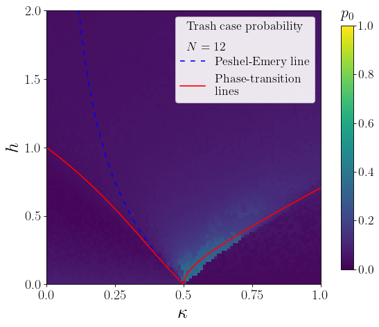
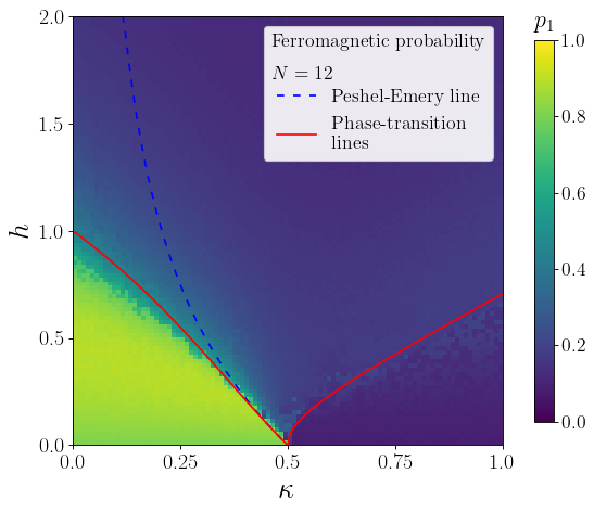
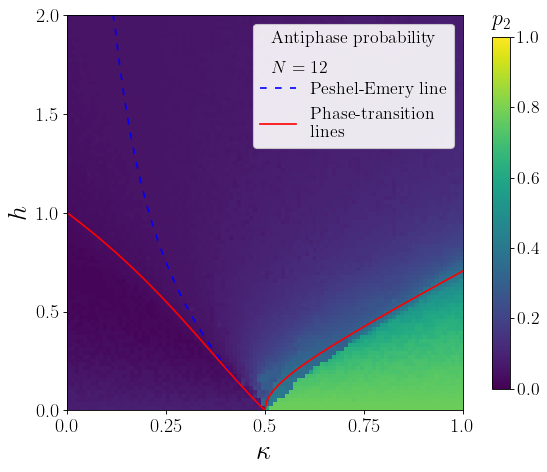
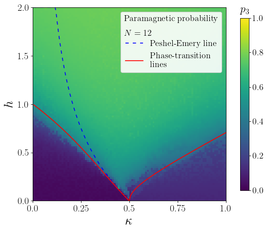
As explained in the result section, the QCNN outputs the probability of obtaining the four two-qubit state and . We associate the first three to the physical ferro-, para-magnetic, and antiphase, while the last one is treated as a garbage class. In the main text, we plot the probability mixture of the three physical phases with a blue-green-yellow color channel. For clarity and completeness, the individual probability with spins are shown in Figure 6, where the color indicates the magnitude of the corresponding probability.
We observe that the probability of being in the garbage class is almost zero, except near the triple point. Moreover, all predicted phase boundaries are sharp, indicating the classifier’s confidence.
Anhang C Anomaly Detection
For the reader’s convenience, we will recall the unsupervised anomaly detection (AD) scheme, initially proposed by Kottmann et al. (2021), to draw the phase diagram of the Bose-Hubbard model. Since it is an unsupervised learning technique, it bypasses the bottleneck of needing classical training labels and is, therefore, an alternative to the approach taken in this letter.
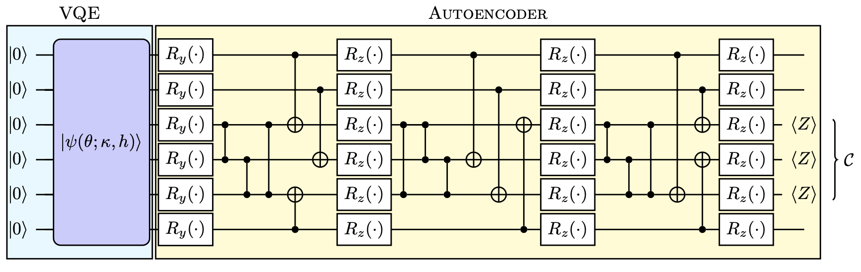
As a first step, an initial state is chosen in the data set composed of the ground states of . Although there is no formal restriction, it should lie far from any critical points. A quantum encoder Romero et al. (2017) is then trained to learn to compress on a -qubit state , with quantum register and , i.e., to write , where the latter is a -qubit trash state with register . The registers here refer to the indices of the qubits composing the states. In practice, an anomaly score based on the Hamming distance between the trash state to , written as
| (4) |
and we make the choice . Intuitively, the encoder compresses similar states, i.e., states in the same phase, with success but will fail to compress states in a different phase, leading to a high anomaly score. The encoder, as proposed in Kottmann et al. (2021), is composed of layers of independent rotations on all qubits and CZi,j gates for and . We use a slightly modified version, with a first layer of individual rotations, followed by layers composed of CXi,j gates for and , CZi,j gates with and independent rotations as displayed in Figure 7 for .
We highlight a few differences with the supervised approach. First, the anomaly score measurement is highly dependent on the choice of the initial state , and can often lead to phase diagrams without any clear phase separation. Moreover, there is no quantitative way to assess the validity of the predicted phase diagram, while with the QCNN, we may evaluate the accuracy on the validation set. Finally, the anomaly score only provided qualitative results. Hence, only a continuous number (the anomaly syndrome) is associated with each point, and there is no canonical way to assign it to a particular phase. On the other hand, the QCNN outputs the probability of being in each phase and therefore, a unique predicted phase can be assigned to each quantum state.