Muon $g-2$ with $SU(2)_{L}$ multiplets

Abstract

We propose a simple model to obtain sizable muon anomalous magnetic dipole moment (muon $g-2$) introducing several $SU(2)_{L}$ multiplet fields without any additional symmetries. The neutrino mass matrix is simply induced via type-II seesaw scenario in terms of $SU(2)_{L}$ triplet Higgs with $U(1)_{Y}$ hypercharge 1. In addition, we introduce an $SU(2)_{L}$ quartet vector fermion with $1/2$ hypercharge and scalar with $3/2$ hypercharge. The quartet fermion plays a crucial role in explaining muon $g-2$ causing the chiral flip inside a loop diagram with mixing between triplet and quartet scalar bosons via the standard model Higgs. We show numerical analysis and search for allowed region in our parameter space, and demonstrate the collider physics.

I Introductions

Even after discovery of the standard model (SM) Higgs, we have to resolve several issues such as non-zero neutrino masses and muon anomalous magnetic dipole moment (muon $g-2$) that would indicate necessity of beyond the SM. New results on the muon $g-2$ are reported by the E989 collaboration at Fermilab Muong-2:2021ojo :

$$a^{\rm FNAL}_{\mu}=116592040(54)\times 10^{-11}.$$ (1)

Furthermore, combined result with the previous BNL, suggests that the muon $g-2$ deviates from the SM prediction by 4.2$\sigma$ level Muong-2:2021ojo ; Aoyama:2012wk ; Aoyama:2019ryr ; Czarnecki:2002nt ; Gnendiger:2013pva ; Davier:2017zfy ; Keshavarzi:2018mgv ; Colangelo:2018mtw ; Hoferichter:2019mqg ; Davier:2019can ; Keshavarzi:2019abf ; Kurz:2014wya ; Melnikov:2003xd ; Masjuan:2017tvw ; Colangelo:2017fiz ; Hoferichter:2018kwz ; Gerardin:2019vio ; Bijnens:2019ghy ; Colangelo:2019uex ; Blum:2019ugy ; Colangelo:2014qya ; Hagiwara:2011af :

$$\Delta a^{\rm new}_{\mu}=(25.1\pm 5.9)\times 10^{-10}.$$ (2)

Although results on the hadron vacuum polarization (HVP), estimated by recent lattice calculations Borsanyi:2020mff ; Alexandrou:2022amy ; Ce:2022kxy , may weaken the necessity of a new physics effect, it is shown in refs. Crivellin:2020zul ; deRafael:2020uif ; Keshavarzi:2020bfy   that the lattice results implies new tensions with the HVP extracted from $e^{+}e^{-}$ data and the global fits to the electroweak precision observables. If muon $g-2$ suggests new physics, we expect new particles and interactions. To explain the sizable muon $g-2$ with natural manner by Yukawa couplings,  we would need one-loop contributions with chiral flip by heavy fermion mass inside a loop diagram Lindner:2016bgg ; Athron:2021iuf ; Guedes:2022cfy . Otherwise, the Yukawa couplings would exceed perturbation limit or too light mediator masses are required.

Simple ways to extend the SM to resolve these issues are introduction of new fields that are $SU(2)_{L}$ multiplets Nomura:2018lsx ; Nomura:2018cfu ; Nomura:2018ibs ; Nomura:2018cle ; Nomura:2017abu ; Nomura:2016jnl ; Nomura:2016dnf ; Cai:2017jrq ; Anamiati:2018cuq ; Guedes:2022cfy ; Calibbi:2018rzv ; Baek:2016kud . For example, neutrino masses can be induced by adding Higgs triplet with hypercharge $1$ that is known as type-II seesaw mechanism Magg:1980ut ; Lazarides:1980nt ; Schechter:1980gr ; Cheng:1980qt ; Mohapatra:1980yp ; Bilenky:1980cx . We can also expect that sizable contribution to muon $g-2$ is obtained by adding a vector-like fermion multiplet in addition to a scalar multiplet where chiral flip occurs inside a loop picking up vector-like fermion mass. Also multiple electric charge of components in large multiplets can enhance muon $g-2$ value. In addition to explaining muon $g-2$ anomaly and neutrino masses, large $SU(2)_{L}$ multiplet fields would induce interesting signatures at collider experiments as it contains multiply-charged particles.

In this paper, we explain the sizable muon $g-2$ via $SU(2)_{L}$ multiplet fields without any additional symmetries. More concretely, we add an $SU(2)_{L}$ quartet vector fermion with $1/2$ hypercharge, one triplet Higgs with $1$ hypercharge, and one quartet scalar with $3/2$ hypercharge. The quartet fermion plays an crucial role in explaining the sizable muon $g-2$ causing the chiral flip in terms of its mass term as well as through mixing between triplet and quartet bosons. In addition, the neutrino mass matrix is simply induced via type-II scenario via the Yukawa interactions between the lepton doublet and triplet Higgs field. Note also that we should consider constraints on vacuum expectation values (VEVs) of $SU(2)_{L}$ multiplet scalar fields since it deviate $\rho$-parameter from $1$. After formulating our model, we show numerical analysis and search for allowed region in our parameter space, and discuss the collider physics focusing on productions of multiply-charged particles in the model.

This paper is organized as follows. In Sec. II, we introduce our model and formulate the Yukawa sector and Higgs sector, oblique $\rho$ parameter, neutral fermion masses including the active neutrino masses, lepton flavor violations (LFVs), and muon $g-2$. In Sec. III, we show numerical analysis of muon $g-2$ and discuss collider physics. Finally we devote the summary of our results and the conclusion.

II Model setup and Constraints

	$L_{L_{i}}$	$e_{R_{i}}$	$\psi$	$H$	$\Delta$	$H_{4}$
$SU(2)_{L}$	$\bm{2}$	$\bm{1}$	$\bm{4}$	$\bm{2}$	$\bm{3}$	$\bm{4}$
$U(1)_{Y}$	$-\frac{1}{2}$	$-1$	$\frac{1}{2}$	${\frac{1}{2}}$	$1$	$\frac{3}{2}$

Table 1: Charge assignments of the our lepton and scalar fields under $SU(2)_{L}\times U(1)_{Y}$, where the lower index $i$ is the number of family that runs over $1-3$, all of them are singlet under $SU(3)_{C}$, and the quark sector is the same as the SM one.

In this section we introduce our model. As for the fermion sector, we introduce one family of vector fermion $\psi$ with $(4,{1/2})$ where each of content in parentheses represents the charge assignment of the SM gauge groups ($SU(2)_{L},U(1)_{Y}$), hereafter. As for the scalar sector, we add a triplet scalar field $\Delta$ with $(3,1)$ which realizes type-II seesaw mechanism and a quartet scalar field $H_{4}$ with $(4,{3/2})$, where SM-like Higgs field is denoted as $H$. Here we write components of multiplets as

$$H=(h^{+},\tilde{h}^{0})$$ (3)

$$\Delta=\begin{pmatrix}\frac{\delta^{+}}{\sqrt{2}}&\delta^{++}\\ \delta^{0}&-\frac{\delta^{+}}{\sqrt{2}}\end{pmatrix},$$ (4)

$$H_{4}=(\phi^{+++}_{4},\phi_{4}^{++},\phi_{4}^{+},\phi_{4}^{0})^{T},$$ (5)

$$\psi_{L(R)}=(\psi^{++},\psi^{+},\psi^{0},\psi^{-})^{T}_{L(R)},$$ (6)

where $\tilde{h}^{0}=\frac{1}{\sqrt{2}}(h^{0}+v_{h}+iG^{0})$ and the triplet can be also written by $H_{3}=(\delta^{0},\delta^{+},\delta^{++})^{T}$. Neutral components of scalar fields develop VEVs denoted by $\{\langle H\rangle,\langle\Delta\rangle,\langle H_{4}\rangle\}\equiv\{v_{h},v_{\Delta},v_{4}\}/\sqrt{2}$ which induce the spontaneous electroweak symmetry breaking. All the field contents and their assignments are summarized in Table 1, where the quark sector is exactly the same as the SM. The renormalizable lepton Yukawa Lagrangian under these symmetries is given by

$$-{\cal L_{\ell}} =y_{\ell_{ii}}\bar{L}_{L_{i}}He_{R_{i}}+y_{\nu_{ij}}\bar{L}_{L_{i}}\Delta^{\dagger}L^{c}_{L_{j}}+y_{D_{i}}[\bar{L}_{L_{i}}\Delta^{\dagger}\psi_{R}]+f_{i}[\bar{\psi}_{L}H_{4}e_{R_{i}}]$$

$$+g_{L}[\bar{\psi}^{c}_{L}\Delta^{\dagger}\psi_{L}]+g_{R}[\bar{\psi}^{c}_{R}\Delta^{\dagger}\psi_{R}]+M_{\psi}\bar{\psi}_{L}\psi_{R}+{\rm h.c.},$$ (7)

where we implicitly symbolize the gauge invariant contracts of $SU(2)_{L}$ index as bracket [$\cdots$] hereafter, indices $(i,j)=1$-$3$ are the number of families, $y_{\ell}$ is assumed to be diagonal matrix with real parameters without loss of generality. Then, the mass eigenvalues of charged-lepton are defined by $m_{\ell}=y_{\ell}v_{h}/\sqrt{2}={\rm Diag}(m_{e},m_{\nu},m_{\tau})$. In our model scalar potential is written by

$$V= -\mu_{H}^{2}H^{\dagger}H+\mu_{\Delta}^{2}{\rm Tr}[\Delta^{\dagger}\Delta]+\mu_{H_{4}}^{2}H^{\dagger}_{4}H_{4}+\lambda_{H}(H^{\dagger}H)^{2}$$

$$+(\text{trivial quartet terms including $\Delta$ and $H_{4}$})+V_{\rm non-trivial},$$ (8)

where we omit details of trivial quartet terms with $\Delta$ and $H_{4}$ for simplicity and assume their couplings are small. The non-trivial scalar potential is given by

$$V_{\rm non-trivial}=\mu_{1}[H^{\dagger}\Delta^{\dagger}H_{4}+{\rm h.c.}]+\mu_{2}[H^{T}\Delta^{\dagger}H]+\sum_{i}\lambda_{H_{4}H}^{i}[H_{4}^{\dagger}HHH]_{i}+{\rm h.c.},$$ (9)

where $\mu_{1}$ plays a crucial role in inducing the muon $g-2$ as can be seen later.

Note that we can generalize $SU(2)_{L}$ representation of $\psi$ and $H_{4}$ to be $\bf{N}$ if it satisfies $\bf{N}\times\bf{3}\times\bf{2}\supset\bf{1}$, in realizing sizable muon $g-2$. Here we chose $\bf{N}=\bf{4}$ although the minimal choice is $\bf{N}=2$ since the choice of $\bf{N}=\bf{4}$ induce interesting phenomenology at the collider experiments as it provides multiply-charged particles inside a multiplet.

II.1 VEVs of scalar fields and $\rho$-parameter

Non-zero VEVs of scalar fields are obtained by solving the stationary conditions

$$\frac{\partial V}{\partial v_{h}}=\frac{\partial V}{\partial v_{\Delta}}=\frac{\partial V}{\partial v_{4}}=0.$$ (10)

Here we explicitly write the first two terms of Eq. (9) by

$$\frac{\mu_{1}}{3\sqrt{2}}(v_{h}+h_{0})(\sqrt{3}\phi^{0}_{4}\delta^{0*}+\sqrt{6}\phi^{+}_{4}\delta^{-}+3\phi^{++}\delta^{--})-\frac{1}{\sqrt{2}}\mu_{2}\delta^{0*}(h^{0}+v_{h})^{2}+c.c.\ ,$$ (11)

where we consider it in unitary gauge. Assuming $v_{4},v_{\Delta}\ll v_{h}$ and small couplings for trivial quartet couplings, we obtain the VEVs approximately as

$$v_{h}\simeq\sqrt{\frac{\mu_{H}^{2}}{\lambda_{H}}},\quad v_{\Delta}\simeq\frac{1}{\mu_{\Delta}^{2}}\left(\frac{1}{3}\sqrt{\frac{3}{2}}\mu_{1}v_{4}v_{h}+\mu_{2}v_{h}^{2}\right),\quad v_{4}\simeq\frac{1}{3}\sqrt{\frac{3}{2}}\frac{\mu_{1}v_{\Delta}v_{h}}{\mu_{H_{4}}^{2}}.$$ (12)

Thus small values of $v_{\Delta}$ and $v_{4}$ are naturally obtained when mass parameters $\mu_{\Delta}$ and $\mu_{H_{4}}$ are larger than electroweak scale.

The electroweak $\rho$ parameter deviates from unity due to the nonzero values of $v_{\Delta}$ and $v_{4}$ at the tree level as follows:

$$\rho=\frac{v_{h}^{2}+2v_{\Delta}^{2}+6v_{4}^{2}}{v_{h}^{2}+4v_{\Delta}^{2}+9v_{4}^{2}},$$ (13)

where the VEVs satisfy the relation $v\equiv\sqrt{v_{h}^{2}+v_{\Delta}^{2}+v_{4}^{2}}\simeq 246$ GeV. Here we consider current constraint on $\rho$ parameter; $\rho=1.00038\pm 0.00020$ ParticleDataGroup:2020ssz . If we take $v_{x}\equiv v_{\Delta}=v_{4}$ the upper bound of $v_{X}$ is

$$v_{X}\lesssim 1.55\ {\rm GeV},$$ (14)

when we require $\rho$ to be within 2$\sigma$ level. In our analysis we choose $v_{\Delta}\sim v_{4}\sim 1$ GeV for simplicity.

II.2 Masses of new particles

The scalars and fermions with large $SU(2)_{L}$ multiplet provide exotic charged particles. The mass terms of $H_{4}$, $\Delta$ and $\psi$ are approximately given by

$$\mathcal{L}_{M}=\mu_{\Delta}^{2}{\rm Tr}[\Delta^{\dagger}\Delta]+\mu_{H_{4}}^{2}H^{\dagger}_{4}H_{4}+\frac{\mu_{1}v_{h}}{3}(\sqrt{3}\phi^{0}_{4}\delta^{0*}+\sqrt{6}\phi^{+}_{4}\delta^{-}+3\phi^{++}\delta^{--}+c.c.)+M_{\psi}\bar{\psi}\psi,$$ (15)

where we ignored contributions from quartet terms in the scalar potential assuming they are small enough. Thus components in $\psi$ have degenerate mass $M_{\psi}$ where small mass shift appears at loop level Cirelli:2005uq but we ignore it in our analysis below. The triply charged scalar mass is given by $m_{H^{+++}}=\mu_{H_{4}}$ while we have $\delta^{\pm}-\phi^{\pm}_{4}$, $\delta^{\pm\pm}-\phi^{\pm\pm}_{4}$, and $\delta^{0}-\phi^{0}_{4}$ mixings through $\mu_{1}$ term that lead to sizable muon $g-2$ as we discuss below. We write mass eigenstates and mixings as follows:

$$\begin{pmatrix}\delta^{\pm}\\ \phi^{\pm}_{4}\end{pmatrix}=\begin{pmatrix}c_{\alpha}&s_{\alpha}\\ -s_{\alpha}&c_{\alpha}\end{pmatrix}\begin{pmatrix}H^{\pm}_{1}\\ H^{\pm}_{2}\end{pmatrix},$$ (16)

$$\begin{pmatrix}\delta^{\pm\pm}\\ \phi^{\pm\pm}_{4}\end{pmatrix}=\begin{pmatrix}c_{\beta}&s_{\beta}\\ -s_{\beta}&c_{\beta}\end{pmatrix}\begin{pmatrix}H^{\pm\pm}_{1}\\ H^{\pm\pm}_{2}\end{pmatrix},$$ (17)

$$\begin{pmatrix}\delta^{0}\\ \phi^{0}_{4}\end{pmatrix}=\begin{pmatrix}c_{\gamma}&s_{\gamma}\\ -s_{\gamma}&c_{\gamma}\end{pmatrix}\begin{pmatrix}H^{0}_{1}\\ H^{0}_{2}\end{pmatrix},$$ (18)

where $c_{a},s_{a}$ are respectively short-hand notation of $\cos a,\sin a$ with $a\equiv(\alpha,\beta,\gamma)$. The mass eigenvalues and mixing angles are given by

$$m^{2}_{\{H_{1}^{+},H_{1}^{++},H_{1}^{0}\}}=\frac{1}{2}(\mu_{H_{4}}^{2}+\mu_{\Delta}^{2})-\frac{1}{2}\sqrt{(\mu_{H_{4}}^{2}-\mu_{\Delta}^{2})^{2}+4\Delta M^{4}_{\{+,++,0\}}},$$ (19)

$$m^{2}_{\{H_{2}^{+},H_{2}^{++},H_{2}^{0}\}}=\frac{1}{2}(\mu_{H_{4}}^{2}+\mu_{\Delta}^{2})+\frac{1}{2}\sqrt{(\mu_{H_{4}}^{2}-\mu_{\Delta}^{2})^{2}+4\Delta M^{4}_{\{+,++,0\}}},$$ (20)

$$\tan(2\{\alpha,\beta,\gamma\})=\frac{2\Delta M^{2}_{\{+,++,0\}}}{\mu_{\Delta}^{2}-\mu_{H_{4}}^{2}},$$ (21)

$$\Delta M^{2}_{\{+,++,0\}}=\left\{\frac{\sqrt{3}\mu_{1}v_{h}}{3},\frac{\sqrt{6}\mu_{1}v_{h}}{3},\mu_{1}v_{h}\right\}.$$ (22)

Notice here that we neglect the mixing between the SM Higgs and other neutral scalar bosons choosing related parameters to be sufficiently small, and we do not discuss experimental constraint related to the SM Higgs boson assuming its couplings are the SM like.

II.3 Neutral fermion masses

After the spontaneous symmetry breaking, neutral fermion mass matrix in basis of $\Psi^{0}_{L}\equiv(\nu_{L}^{c},\psi_{R},\psi_{L}^{c})^{T}$ is given by

$$M_{N} =\left[\begin{array}[]{ccc}m_{\nu}^{(II)}&m_{D}&0\\ m_{D}^{T}&m_{R}&M_{\psi}\\ 0&M_{\psi}&m_{L}\\ \end{array}\right],$$ (26)

where $m_{\nu}^{(II)}\equiv y_{\nu}v_{\Delta}$, $m_{D}\equiv{y_{D}v_{\Delta}}/\sqrt{3}$, $m_{R}\equiv{2g_{R}v_{\Delta}}/3$, and $m_{L}\equiv{2g_{L}v_{\Delta}}/3$. Achieving the block diagonalizing, we find the active neutrino mass matrix:

$$m_{\nu}\approx m_{\nu}^{(II)}+\frac{m_{D}m_{D}^{T}m_{L}}{M^{2}_{\psi}}.$$ (27)

The second term in the above equation corresponds to inverse seesaw, but its matrix rank is one. Thus, we simply expect that the neutrino oscillation data is dominantly described by the first term $m_{\nu}^{(II)}$. Notice here that we need the following constraint to achieve $m_{\nu}\approx m_{\nu}^{(II)}$;

$$\frac{m_{D}m_{D}^{T}m_{L}}{M^{2}_{\psi}}<<0.1\ {\rm eV}.$$ (28)

Here, we assume $m_{D}$ to be negligibly tiny in order to evade the mixing between the SM charged-leptons and the exotic charged fermions. In this case, there is no mixing between the active neutrinos and heavier neutral fermions also. Thus, the heavier neutral mass eigenvalues diag[$D_{1},D_{2}$] are given by unitary matrix $V_{N}$ as $D=V_{N}M_{N}V_{N}^{T}$ where

$$M_{N} =\left[\begin{array}[]{cc}m&M_{\psi}\\ M_{\psi}&m\\ \end{array}\right],$$ (31)

$$D_{1} =M_{\psi}-m,\ D_{2}=M_{\psi}+m,$$ (32)

$$V_{N} =\frac{1}{\sqrt{2}}\left[\begin{array}[]{cc}i&0\\ 0&1\\ \end{array}\right]\left[\begin{array}[]{cc}1&-1\\ 1&1\\ \end{array}\right].$$ (37)

Here we assume $m\equiv m_{R}=m_{L}$ for simplicity.

The active neutrino mass matrix is diagonalized by $D_{\nu}=U_{\rm MNS}m_{\nu}U_{\rm MNS}^{T}$ where $U_{\rm MNS}$ is Maki Nakagawa Sakata mixing matrix ParticleDataGroup:2020ssz . It suggests that we simply parametrize $y_{\nu}$ as follows:

$$y_{\nu}=\frac{1}{v_{\Delta}}U_{\rm MNS}^{\dagger}D_{\nu}U_{\rm MNS}^{T}.$$ (38)

Basically we can realize neutrino mass and mixing tuning Yukawa couplings $y_{\nu_{ij}}$ same as the type-II seesaw mechanism. Thus we do not discuss neutrino masses further in this paper.

II.4 Lepton flavor violations(LFVs) and muon $g-2$

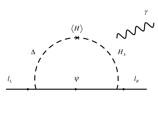
Figure 1: Feynman diagram to generate muon $g-2$ and $\ell\to\ell^{\prime}\gamma$ processes.

In our model LFV processes and muon $g-2$ are induced from Yukawa interactions associated with couplings $\{y_{D},\ f\}$. The relevant terms are explicitly written by

$$f_{i}[\overline{\psi_{L}}H_{4}e_{R_{i}}]+y_{D_{i}}[\overline{L_{L_{i}}}\Delta^{\dagger}\psi_{R}]+h.c.$$

$$\quad=f_{i}[\overline{\psi^{0}_{L}}\phi^{+}_{4}+\overline{\psi^{++}_{L}}\phi^{+++}_{4}+\overline{\psi^{+}_{L}}\phi^{++}_{4}+\overline{\psi^{-}_{L}}\phi^{0}_{4}]e_{R_{i}}$$ (39)

$$\quad+\frac{y_{D_{i}}}{3}[\overline{e_{R_{i}}}(\sqrt{3}\delta^{0*}\psi^{-}_{R}+3\delta^{--}\psi^{+}_{R}+\sqrt{6}\delta^{-}\psi^{0}_{R})+\overline{\nu_{L_{i}}}(\sqrt{3}\delta^{0*}\psi_{R}^{0}+3\delta^{--}\psi^{++}_{R}+\sqrt{6}\delta^{-}\psi^{+}_{R})].$$

Considering scalar mixing in Eqs. (16)-(18) contributions to $\ell\to\ell^{\prime}\gamma$ and muon $g-2$ are given by one-loop diagram in Fig. 1. Branching ratios (BRs) of LFV processes are written by the following formula;

$${\rm BR}(\ell_{i}\to\ell_{j}\gamma)=\frac{48\pi^{3}\alpha_{\rm em}C_{ij}}{(4\pi)^{4}{\rm G_{F}^{2}}m_{\ell_{i}}^{2}}\left(|a_{R_{ij}}|^{2}+|a_{L_{ij}}|^{2}\right).$$ (40)

Dominant contributions to amplitudes $a_{L}$ and $a_{R}$ are given by

$$a_{R_{ji}} =-y_{D_{j}}f_{i}(-1)^{k-1}\left[\frac{\sqrt{6}s_{\alpha}c_{\alpha}}{3}D_{a}F(m_{c_{k}},D_{a})\right.$$

$$\left.+M_{\psi}\left(s_{\beta}c_{\beta}\left(F(m_{d_{k}},M_{\psi})-G(m_{d_{k}},M_{\psi})\right)+\frac{s_{\gamma}c_{\gamma}}{\sqrt{3}}G(m_{h_{k}},M_{\psi})\right)\right],$$ (41)

$$a_{L_{ji}} =-f^{\dagger}_{j}y^{\dagger}_{D_{i}}(-1)^{k-1}\left[\frac{\sqrt{6}s_{\alpha}c_{\alpha}}{3}D_{a}F(m_{c_{k}},D_{a})\right.$$

$$\left.+M_{\psi}\left(s_{\beta}c_{\beta}\left(F(m_{d_{k}},M_{\psi})-G(m_{d_{k}},M_{\psi})\right)+\frac{s_{\gamma}c_{\gamma}}{\sqrt{3}}G(m_{h_{k}},M_{\psi})\right)\right],$$ (42)

where $a,k$ runs over $1,2$, and the loop functions are

$$F(m_{a},m_{b})\approx\frac{m_{a}^{4}-m_{b}^{4}+2m_{a}^{2}m_{b}^{2}\ln\left(\frac{m_{b}^{2}}{m_{a}^{2}}\right)}{2(m_{a}^{2}-m_{b}^{2})^{3}},$$ (43)

$$G(m_{a},m_{b})\approx-\frac{3m_{a}^{4}+m_{b}^{4}-4m_{a}^{2}m_{b}^{2}+2m_{a}^{4}\ln\left(\frac{m_{b}^{2}}{m_{a}^{2}}\right)}{2(m_{a}^{2}-m_{b}^{2})^{3}}.$$ (44)

The current experimental upper bounds on BRs of LFV processes are given by MEG:2016leq ; MEG:2013oxv

$${\rm BR}(\mu\rightarrow e\gamma) \leq 4.2\times 10^{-13},\quad{\rm BR}(\tau\rightarrow\mu\gamma)\leq 4.4\times 10^{-8},\quad{\rm BR}(\tau\rightarrow e\gamma)\leq 3.3\times 10^{-8}~{}.$$ (45)

We impose these constraints in our numerical analysis below.

Muon $g-2$; $\Delta a_{\mu}$, arises from the same diagram as LFVs and it is formulated by the following expression:

$$\Delta a_{\mu}\approx-\frac{m_{\mu}}{(4\pi)^{2}}[{a_{L_{22}}+a_{R_{22}}}].$$ (46)

The recent data tells us $\Delta a_{\mu}=(25.1\pm 5.9)\times 10^{-10}$ Muong-2:2021ojo at 1$\sigma$ C.L.. Note that $a_{L,R}$ does not have chiral suppression since vector-like lepton mass $M_{\psi}$ is picked up inside loop. The simplest way to obtain the sizable muon $g-2$ is to set $f_{1,3}=y_{D_{1,3}}=0$, taking $f_{2}$ and $y_{D_{2}}$ to be order one. Then, we do not need to consider the constraints of LFVs. In the next subsection, we will show how it works through numerical analysis.

III Numerical analysis and phenomenology

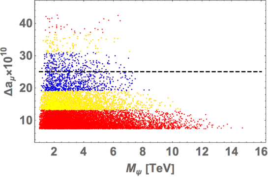
Figure 2: Random plot of muon $g-2$ in terms of mass parameter $M_{\psi}$ within the range of Eq. (47) where we imposed LFV constraints. The black dashed line represents the best fit value of muon $g-2$, the blue points are within 1$\sigma$, the yellow ones are within 2$\sigma$, and red ones are within 3$\sigma$ of experimental value.

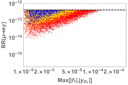
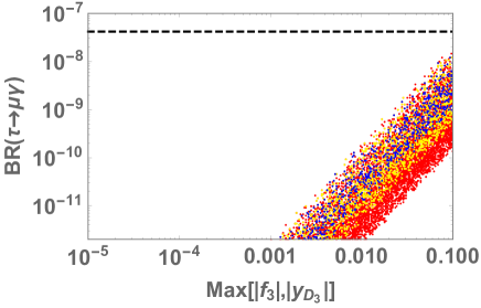
Figure 3: Left and right plots show $BR(\mu\to e\gamma)$ and $BR(\tau\to\mu\gamma)$ as functions of Max$[|f_{1}|,|y_{D_{1}}|]$ and Max$[|f_{3}|,|y_{D_{3}}|]$ for parameter sets satisfying muon $g-2$ within $3\sigma$; the color of points is the same as in Fig. 2. The horizontal dashed line indicates current upper bound of the BRs.

In this section we carry out numerical analysis by scanning free parameters and explore the region to explain muon $g-2$ taking into account LFV constraints. Then we consider collider physics focusing on production of multiply-charged fermions and scalar bosons.

III.1 Numerical analyses on muon $g-2$

Now that the formalulations have been done, we carry out numerical analysis taking into account LFV constraints and muon $g-2$. At first, we randomly select the following input parameters:

$$M_{\psi}\supset[10^{3},10^{5}]\ {\rm GeV},\quad m\supset[0.01,10]\ {\rm GeV},\quad\mu_{H_{4}}=1.2M_{\psi},\quad\mu_{\Delta}=0.8M_{\psi},$$

$$\mu_{1}\supset[100,\mu_{H_{4}}]\ {\rm GeV},\quad\{|f_{2}|,|y_{D_{2}}|\}\supset[0.1,2.0],\quad\{|f_{1,3}|,|y_{D_{1,3}}|\}\supset[10^{-5},0.1],$$ (47)

where we chose $|f_{2}|$ and $|y_{D_{2}}|$ to be larger than other Yukawa couplings so that we have sizable muon $g-2$. Note that splittings of masses of components in the same scalar multiplets are small and we can evade the constraints from oblique parameters Peskin:1990zt .

Fig. 2 represents the values of muon $g-2$ in terms of mass parameter $M_{\psi}$ where each point corresponds to one parameter sets within the range of Eq. (47) allowed by LFV constraints that satisfy a value of muon $g-2$ in $3\sigma$. The black dashed line shows the best fit value of muon $g-2$, the blue points are within 1$\sigma$, the yellow ones are within 2$\sigma$, and red ones are within 3$\sigma$ of experimental value. We thus find that $M_{\psi}\lesssim 15(8.5)$ TeV is preferred to obtain muon $g-2$ within $3(1)\sigma$ C.L. in our scenario. In addition we show branching ratios of LFV processes for the same parameter sets in Fig. 3 where the left and right plots represent $BR(\mu\to e\gamma)$ and $BR(\tau\to\mu\gamma)$ as functions of Max$[|f_{1}|,|y_{D_{1}}|]$ and Max$[|f_{3}|,|y_{D_{3}}|]$, and the color of points is the same as Fig. 2. It is found that $|f_{1}|(|y_{D_{1}}|)$ should be smaller than $\sim 10^{-4}$ to avoid stringent constraint from $BR(\mu\to e\gamma)$ while constraint on $f_{3}(y_{D_{3}})$ is much looser. Here we omitted a plot for $BR(\tau\to e\gamma)$ since it is not correlated to muon $g-2$ and it tends to be much smaller than experimental limit.

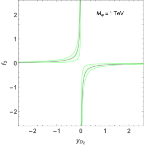
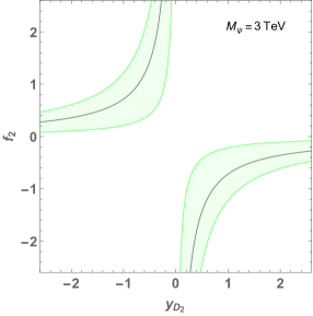
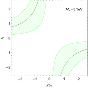
Figure 4: The region realizing muon $g-2$ within 3$\sigma$ C.L. for $M_{\psi}=\{1,3,5\}$ TeV on $\{y_{D_{2}},f_{2}\}$ plane where we chose $\mu_{1}=\mu_{H_{4}}=1.2M_{\psi}$, $\mu_{\Delta}=0.8M_{\psi}$, $m=10$ GeV and $y_{D_{1,3}}=f_{1,3}=0$. The parameters on the black curve provide best fit value of the muon $g-2$.

Next, we also demonstrate a simple realization to get sizable muon $g-2$ setting $f_{1,3}=y_{D_{1,3}}=0$, taking $f_{2}$ and $y_{D_{2}}$ to be free parameters. This is because we can enhance the muon $g-2$ without inducing LFVs. Fig. 4 represents region realizing muon $g-2$ within $3\sigma$ C.L. on the parameter space of the valid Yukawa coupling $y_{D_{2}}$ and $f_{2}$ fixing the other input parameters as follows; $M_{\psi}=\{1,3,5\}$ TeV as indicated on the plots, $\mu_{H_{4}}=1.2M_{\psi}$, $\mu_{\Delta}=0.8M_{\psi}$, $m=10$ GeV, and $\mu_{1}=\mu_{H_{4}}$. The black solid curves represent the parameter region providing the best fit value of muon $g-2$. One finds that less than order one Yukawa couplings are enough to find the best fit value of muon $g-2$ even when the fermion mass is of the order 3 TeV.

III.2 collider physics

Here we briefly discuss collider signature of the model focusing on the pair productions of new particles with the highest electric charge in $H_{4}$ and $\psi$. They can be produced via electroweak gauge interactions that are given by

$$(D_{\mu}H_{4})^{\dagger}(D^{\mu}H_{4})\supset i\left[\frac{g}{c_{W}}\left(\frac{3}{2}-3s^{2}_{W}\right)Z_{\mu}+3eA_{\mu}\right](\partial^{\mu}H^{+++}H^{---}-\partial^{\mu}H^{---}H^{+++})$$ (48)

$$\bar{\psi}i\gamma^{\mu}D_{\mu}\psi\supset\overline{\psi^{++}}\gamma^{\mu}\left[\frac{g}{c_{W}}\left(\frac{3}{2}-2s^{2}_{W}\right)+2eA_{\mu}\right]\psi^{++},$$ (49)

where we omitted other terms which are irrelevant in our calculation below. We consider the production processes

$$pp\to Z/\gamma\to H^{+++}H^{---},$$ (50)

$$pp\to Z/\gamma\to\overline{\psi^{++}}\psi^{++},$$ (51)

in a hadron collider experiment. Here we estimate the production cross sections in use of CalcHEP 3.8 Belyaev:2012qa package implementing the relevant interactions applying the CTEQ6 parton distribution functions (PDFs) Nadolsky:2008zw . In Fig. 5, the cross sections are shown as functions of exotic charged particle masses for center of mass energy $\sqrt{s}=14,27$ and 100 TeV as reference values. We find that $\overline{\psi^{++}}\psi^{++}$ production cross section is larger than that of $H^{+++}H^{---}$ by one order.

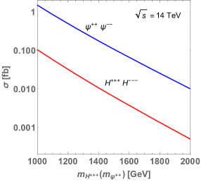
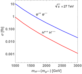
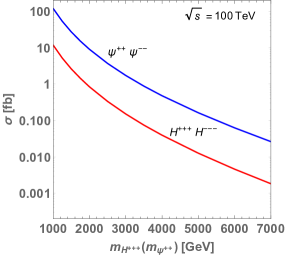
Figure 5: Cross sections for $pp\to H^{+++}H^{---}$ and $pp\to\psi^{++}\psi^{--}$ with center of mass energy 14 TeV, 27 TeV and 100 TeV.

Exotic changed particles can decay via Yukawa couplings in Eq. (7). Here we assume relation among mass parameters as $\mu_{\Delta}<M_{\psi}<\mu_{H_{4}}$ for illustration. Then dominant decay modes of $H^{+++}$ and $\psi^{++}$ are respectively $H^{+++}\to\ell^{+}\psi^{++}$ and $\psi^{++}\to\nu_{\ell}\delta^{++}$ where the decay widths are given by

$$\Gamma(H^{+++}\to\ell^{+}\psi^{+++}) =\frac{f_{\ell}^{2}}{16\pi}m_{H^{+++}}\left(1-\frac{M_{\psi}^{2}}{m^{2}_{H^{+++}}}\right)^{2},$$ (52)

$$\Gamma(\psi^{++}\to\nu_{\ell}\delta^{++}) =\frac{y_{\ell}^{2}}{8\pi}M_{\psi}.$$ (53)

Note that here we consider $\delta^{++}\simeq H_{1}^{++}$ assuming small mixing angle for simplicity. In addition $\delta^{++}$ dominantly decays into $W^{+}W^{+}$ mode considering $v_{\Delta}\sim\mathcal{O}(1)$ GeV. Thus decay chains provide signature from $H^{+++}H^{---}$ and $\psi^{++}\psi^{--}$ such that

$$\psi^{++}\overline{\psi^{++}}\to\nu\bar{\nu}\delta^{++}\delta^{--}\to\nu\bar{\nu}W^{+}W^{+}W^{-}W^{-},$$ (54)

$$H^{+++}H^{---}\to\ell^{+}\ell^{-}\psi^{++}\overline{\psi^{++}}\to\ell^{+}\ell^{-}\nu\bar{\nu}\delta^{++}\delta^{--}\to\ell^{+}\ell^{-}\nu\bar{\nu}W^{+}W^{+}W^{-}W^{-},$$ (55)

where $\nu(\bar{\nu})$ indicates any flavor of neutrino (anti-neutrino). For signals, we consider one pair of same sign $W$ bosons decays into leptons while the other same sign pair decays into jets. The signals at detectors are

$$\text{Signal 1:}\quad\ell^{\pm}\ell^{\pm}4j\not{E}_{T},$$ (56)

$$\text{Signal 2:}\quad\ell^{\pm}\ell^{\pm}\ell^{\pm}\ell^{\mp}4j\not{E}_{T},$$ (57)

where $j$ and $\not{E}_{T}$ indicate jet and missing transverse momentum. In Table 2, we provide expected number of events for some benchmark points (BPs) of $M_{\psi}(m_{H^{+++}})$ assuming integrated luminosity of $L=1$ ab^-1 and $m_{\delta^{++}}<M_{\psi}$ to allow the decay mode of $\psi^{++}\to\delta^{++}\nu$. Note that the number of SM background event will be very small by tagging the same sign charged leptons in final states. We thus find that mass scale of around 1 to 2 TeV can be explored by $\sqrt{s}=14$ TeV with sufficient integrated luminosity that will be achieved by High-Luminosity-LHC experiment. In addition most of mass region explaining muon $g-2$ could be tested if we realize a higher energy experiment like 100 TeV collider in future FCC:2018byv .

$\sqrt{s}$ [TeV]	14				27				100
$M_{\psi}(m_{H^{+++}})$ [GeV]	1000	1250	1500	1750	1000	1500	2000	2500	2000	3000	4000	6000
# of events [Signal 1]	324.	82.	23.	7.	2221.	319.	65.	16.	1954.	373.	103.	14.
# of events [Signal 2]	22.	5.	1.	0.	188.	24.	4.	1.	181.	33.	8.	1.

Table 2: Expected number of events for our signals in some BPs of $M_{\psi}(m_{H^{+++}}$) with integrated luminosity of $L=1$ ab^-1.

IV Summary and discussion

In this paper we have proposed a simple extension of the SM without additional symmetry by introducing large $SU(2)_{L}$ multiplet fields such as quartet vector-like fermion as well as quartet and triplet scalar fields. These multiplet fields can induce sizable muon $g-2$ due to new Yukawa couplings at one-loop level where we do not have chiral suppression by light lepton mass as we pick up heavy fermion mass term changing chirality inside a loop diagram. The triplet scalar field can induce neutrino masses after developing its VEV by type-II seesaw mechanism.

We have carried out numerical analysis searching for parameter space that explains muon $g-2$ and allowed by LFV constraints. It has been then found that muon $g-2$ can be explained when the new multiplets mass scale are less than around $\mathcal{O}(10)$ TeV. We also discussed collider physics focusing on production of multiply-charged fermions/scalars via proton-proton collision. Mass scale of 1 to 2 TeV can be explored by $\sqrt{s}=14$ TeV with sufficient integrated luminosity that will be achieved by High-Luminosity-LHC experiment. Also most of mass region explaining muon $g-2$ could be tested if we realize a higher energy experiment like 100 TeV collider.

References

• (1) B. Abi et al. [Muon g-2], Phys. Rev. Lett. 126 (2021) no.14, 141801 doi:10.1103/PhysRevLett.126.141801 [arXiv:2104.03281 [hep-ex]].
• (2) K. Hagiwara, R. Liao, A. D. Martin, D. Nomura and T. Teubner, J. Phys. G 38, 085003 (2011) [arXiv:1105.3149 [hep-ph]].
• (3) T. Aoyama, M. Hayakawa, T. Kinoshita and M. Nio, Phys. Rev. Lett. 109, 111808 (2012) doi:10.1103/PhysRevLett.109.111808 [arXiv:1205.5370 [hep-ph]].
• (4) T. Aoyama, T. Kinoshita and M. Nio, Atoms 7, no.1, 28 (2019) doi:10.3390/atoms7010028
• (5) A. Czarnecki, W. J. Marciano and A. Vainshtein, Phys. Rev. D 67, 073006 (2003) [erratum: Phys. Rev. D 73, 119901 (2006)] doi:10.1103/PhysRevD.67.073006 [arXiv:hep-ph/0212229 [hep-ph]].
• (6) C. Gnendiger, D. Stöckinger and H. Stöckinger-Kim, Phys. Rev. D 88, 053005 (2013) doi:10.1103/PhysRevD.88.053005 [arXiv:1306.5546 [hep-ph]].
• (7) A. Keshavarzi, D. Nomura and T. Teubner, Phys. Rev. D 97, no.11, 114025 (2018) doi:10.1103/PhysRevD.97.114025 [arXiv:1802.02995 [hep-ph]].
• (8) G. Colangelo, M. Hoferichter and P. Stoffer, JHEP 02, 006 (2019) doi:10.1007/JHEP02(2019)006 [arXiv:1810.00007 [hep-ph]].
• (9) M. Hoferichter, B. L. Hoid and B. Kubis, JHEP 08, 137 (2019) doi:10.1007/JHEP08(2019)137 [arXiv:1907.01556 [hep-ph]].
• (10) A. Keshavarzi, D. Nomura and T. Teubner, Phys. Rev. D 101, no.1, 014029 (2020) doi:10.1103/PhysRevD.101.014029 [arXiv:1911.00367 [hep-ph]].
• (11) A. Kurz, T. Liu, P. Marquard and M. Steinhauser, Phys. Lett. B 734, 144-147 (2014) doi:10.1016/j.physletb.2014.05.043 [arXiv:1403.6400 [hep-ph]].
• (12) K. Melnikov and A. Vainshtein, Phys. Rev. D 70, 113006 (2004) doi:10.1103/PhysRevD.70.113006 [arXiv:hep-ph/0312226 [hep-ph]].
• (13) P. Masjuan and P. Sanchez-Puertas, Phys. Rev. D 95, no.5, 054026 (2017) doi:10.1103/PhysRevD.95.054026 [arXiv:1701.05829 [hep-ph]].
• (14) G. Colangelo, M. Hoferichter, M. Procura and P. Stoffer, JHEP 04, 161 (2017) doi:10.1007/JHEP04(2017)161 [arXiv:1702.07347 [hep-ph]].
• (15) M. Hoferichter, B. L. Hoid, B. Kubis, S. Leupold and S. P. Schneider, JHEP 10, 141 (2018) doi:10.1007/JHEP10(2018)141 [arXiv:1808.04823 [hep-ph]].
• (16) A. Gérardin, H. B. Meyer and A. Nyffeler, Phys. Rev. D 100, no.3, 034520 (2019) doi:10.1103/PhysRevD.100.034520 [arXiv:1903.09471 [hep-lat]].
• (17) J. Bijnens, N. Hermansson-Truedsson and A. Rodríguez-Sánchez, Phys. Lett. B 798, 134994 (2019) doi:10.1016/j.physletb.2019.134994 [arXiv:1908.03331 [hep-ph]].
• (18) G. Colangelo, F. Hagelstein, M. Hoferichter, L. Laub and P. Stoffer, JHEP 03, 101 (2020) doi:10.1007/JHEP03(2020)101 [arXiv:1910.13432 [hep-ph]].
• (19) T. Blum, N. Christ, M. Hayakawa, T. Izubuchi, L. Jin, C. Jung and C. Lehner, Phys. Rev. Lett. 124, no.13, 132002 (2020) doi:10.1103/PhysRevLett.124.132002 [arXiv:1911.08123 [hep-lat]].
• (20) G. Colangelo, M. Hoferichter, A. Nyffeler, M. Passera and P. Stoffer, Phys. Lett. B 735, 90-91 (2014) doi:10.1016/j.physletb.2014.06.012 [arXiv:1403.7512 [hep-ph]].
• (21) M. Davier, A. Hoecker, B. Malaescu and Z. Zhang, Eur. Phys. J. C 77, no.12, 827 (2017) doi:10.1140/epjc/s10052-017-5161-6 [arXiv:1706.09436 [hep-ph]].
• (22) M. Davier, A. Hoecker, B. Malaescu and Z. Zhang, Eur. Phys. J. C 80, no.3, 241 (2020) [erratum: Eur. Phys. J. C 80, no.5, 410 (2020)] doi:10.1140/epjc/s10052-020-7792-2 [arXiv:1908.00921 [hep-ph]].
• (23) S. Borsanyi, Z. Fodor, J. N. Guenther, C. Hoelbling, S. D. Katz, L. Lellouch, T. Lippert, K. Miura, L. Parato and K. K. Szabo, et al. Nature 593 (2021) no.7857, 51-55 doi:10.1038/s41586-021-03418-1 [arXiv:2002.12347 [hep-lat]].
• (24) C. Alexandrou, S. Bacchio, P. Dimopoulos, J. Finkenrath, R. Frezzotti, G. Gagliardi, M. Garofalo, K. Hadjiyiannakou, B. Kostrzewa and K. Jansen, et al. [arXiv:2206.15084 [hep-lat]].
• (25) M. Cè, A. Gérardin, G. von Hippel, R. J. Hudspith, S. Kuberski, H. B. Meyer, K. Miura, D. Mohler, K. Ottnad and P. Srijit, et al. [arXiv:2206.06582 [hep-lat]].
• (26) A. Crivellin, M. Hoferichter, C. A. Manzari and M. Montull, arXiv:2003.04886 [hep-ph].
• (27) E. de Rafael, Phys. Rev. D 102 (2020) no.5, 056025 [arXiv:2006.13880 [hep-ph]].
• (28) A. Keshavarzi, W. J. Marciano, M. Passera and A. Sirlin, Phys. Rev. D 102 (2020) no.3, 033002 doi:10.1103/PhysRevD.102.033002 [arXiv:2006.12666 [hep-ph]].
• (29) M. Passera, W. J. Marciano and A. Sirlin, Phys. Rev. D 78 (2008), 013009 [arXiv:0804.1142 [hep-ph]].
• (30) W. Altmannshofer, S. Gori, M. Pospelov and I. Yavin, Phys. Rev. Lett. 113 (2014), 091801 doi:10.1103/PhysRevLett.113.091801 [arXiv:1406.2332 [hep-ph]].
• (31) P. Athron, C. Balázs, D. H. J. Jacob, W. Kotlarski, D. Stöckinger and H. Stöckinger-Kim, JHEP 09 (2021), 080 doi:10.1007/JHEP09(2021)080 [arXiv:2104.03691 [hep-ph]].
• (32) M. Lindner, M. Platscher and F. S. Queiroz, Phys. Rept.  731, 1 (2018) [arXiv:1610.06587 [hep-ph]].
• (33) G. Guedes and P. Olgoso, [arXiv:2205.04480 [hep-ph]].
• (34) S. Baek, T. Nomura and H. Okada, Phys. Lett. B 759, 91 (2016) [arXiv:1604.03738 [hep-ph]].
• (35) T. Nomura and H. Okada, Phys. Dark Univ. 26 (2019), 100359 doi:10.1016/j.dark.2019.100359 [arXiv:1808.05476 [hep-ph]].
• (36) T. Nomura and H. Okada, Phys. Rev. D 99 (2019) no.5, 055027 doi:10.1103/PhysRevD.99.055027 [arXiv:1807.04555 [hep-ph]].
• (37) G. Anamiati, O. Castillo-Felisola, R. M. Fonseca, J. C. Helo and M. Hirsch, JHEP 12 (2018), 066 doi:10.1007/JHEP12(2018)066 [arXiv:1806.07264 [hep-ph]].
• (38) T. Nomura and H. Okada, Phys. Rev. D 99 (2019) no.5, 055033 doi:10.1103/PhysRevD.99.055033 [arXiv:1806.07182 [hep-ph]].
• (39) T. Nomura and H. Okada, Phys. Lett. B 783, 381 (2018) [arXiv:1805.03942 [hep-ph]].
• (40) L. Calibbi, R. Ziegler and J. Zupan, JHEP 07 (2018), 046 doi:10.1007/JHEP07(2018)046 [arXiv:1804.00009 [hep-ph]].
• (41) T. Nomura and H. Okada, Phys. Rev. D 96, no. 9, 095017 (2017) [arXiv:1708.03204 [hep-ph]].
• (42) Y. Cai, J. Herrero-García, M. A. Schmidt, A. Vicente and R. R. Volkas, Front. in Phys. 5 (2017), 63 doi:10.3389/fphy.2017.00063 [arXiv:1706.08524 [hep-ph]].
• (43) T. Nomura, H. Okada and Y. Orikasa, Phys. Rev. D 94, no. 5, 055012 (2016) [arXiv:1605.02601 [hep-ph]].
• (44) T. Nomura, H. Okada and Y. Orikasa, Phys. Rev. D 94, no. 11, 115018 (2016) [arXiv:1610.04729 [hep-ph]].
• (45) M. Magg and C. Wetterich, Phys. Lett. B 94, 61 (1980).
• (46) G. Lazarides, Q. Shafi and C. Wetterich, Nucl. Phys. B 181, 287 (1981).
• (47) J. Schechter and J. W. F. Valle, Phys. Rev. D 22, 2227 (1980).
• (48) T. P. Cheng and L. -F. Li, Phys. Rev. D 22, 2860 (1980).
• (49) R. N. Mohapatra and G. Senjanovic, Phys. Rev. D 23, 165 (1981).
• (50) S. M. Bilenky, J. Hosek and S. T. Petcov, Phys. Lett. B 94, 495 (1980).
• (51) P. A. Zyla et al. [Particle Data Group], PTEP 2020 (2020) no.8, 083C01 doi:10.1093/ptep/ptaa104
• (52) M. Cirelli, N. Fornengo and A. Strumia, Nucl. Phys. B 753, 178 (2006) [hep-ph/0512090].
• (53) M. E. Peskin and T. Takeuchi, Phys. Rev. Lett. 65 (1990), 964-967 doi:10.1103/PhysRevLett.65.964
• (54) A. M. Baldini et al. [MEG], Eur. Phys. J. C 76 (2016) no.8, 434 doi:10.1140/epjc/s10052-016-4271-x [arXiv:1605.05081 [hep-ex]].
• (55) J. Adam et al. [MEG], Phys. Rev. Lett. 110 (2013), 201801 doi:10.1103/PhysRevLett.110.201801 [arXiv:1303.0754 [hep-ex]].
• (56) A. Belyaev, N. D. Christensen and A. Pukhov, Comput. Phys. Commun.  184, 1729 (2013) [arXiv:1207.6082 [hep-ph]].
• (57) P. M. Nadolsky, H. L. Lai, Q. H. Cao, J. Huston, J. Pumplin, D. Stump, W. K. Tung and C.-P. Yuan, Phys. Rev. D 78, 013004 (2008) [arXiv:0802.0007 [hep-ph]].
• (58) A. Abada et al. [FCC], Eur. Phys. J. C 79 (2019) no.6, 474 doi:10.1140/epjc/s10052-019-6904-3