Matrix Quantile Factor Model
Abstract
This paper introduces a matrix quantile factor model for matrix-valued data with a low-rank structure. We estimate the row and column factor spaces via minimizing the empirical check loss function over all panels. We show the estimates converge at rate in average Frobenius norm, where , and are the row dimensionality, column dimensionality and length of the matrix sequence. This rate is faster than that of the quantile estimates via “flattening” the matrix model into a large vector model. Smoothed estimates are given and their central limit theorems are derived under some mild condition. We provide three consistent criteria to determine the pair of row and column factor numbers. Extensive simulation studies and an empirical study justify our theory.
Key words: Two-way factor model; Row factor space; Column factor space; Check loss function
JEL Classification: C13, C31, C38
1 Introduction
The present paper studies the matrix sequence data with a latent low-rank structure. Instead of modeling the mean conditional on the latent factors as in recent works (Wang et al. (2019); Yu et al. (2022); Chen and Fan (2021);Gao et al. (2021)), we model the conditional quantiles by an interactive effect of the row and column sections. The parameters (row and column factor loadings and factor matrices) are learnt by minimizing the empirical check loss accumulated over all entries. For the first time, we derived the statistical accuracy results of the estimated factor loading matrices and the factor matrices, under some mild conditions. In the modeling side, this is essentially a work where the matrix factor structure meets the quantile feature representation.
On the matrix factor structure, we assume in the present paper that each matrix observation is driven by a much lower dimensional factor matrix, and that the two cross sections along the row and column dimensions interact with each other and thus generates the entries of the -th data matrix . For example, in recommending system, is a rating matrix of customers and commodities, and the scores in are high when the latent common consumption preferences of the customers match the latent common features of the goods. We focus on matrix sequence rather than large vectors appeared in standard statistics and econometrics for two-fold reasons. First, many recent data sets in financial market, recommending system, social networks, international trade, and electronic business platform, are themselves well collected or organized intrinsically in matrices (or more generally in the form of tensors). The matrix factor structure is empirically found in these data sets and works well in applications, c.f, Chen and Chen (2020) for world trade data analysis. Second, modeling the matrix-value data with a low-rank structure, e.g. (2) below, makes the model parsimonious and statistical inference efficient once the structure is interpretably reasonable. A naive approach to analyze the data matrix is to “flatten” it into a long vector by piling down it column by column or row by row. After that, existing vector sequence models and inference procedures, like the vector factor models in Stock and Watson (2002a), Stock and Watson (2002b), Bai and Ng (2002), Bai (2003), Trapani (2018), Barigozzi and Trapani (2020), Fan et al. (2013), Aït-Sahalia and Xiu (2017), Kong (2017), Kong (2018), Kong et al. (2019), Onatski (2010), Pelger (2019) and Chen et al. (2021), can be applied. However, the flattened vector factor modeling easily misses the interplay between the row and column sections, and has parameter complexity of order while the row-column interaction model (see (2) below) of order . This is also where the efficiency gain of the present paper comes from compared with the vector quantile factor modeling. For more detailed motivation to study matrix or tensor sequence data, we referred to recent interesting works: Chang et al. (2023),Han et al. (2021),Wang et al. (2019), Chen et al. (2020), Chen et al. (2022), Chen et al. (2023) and Zhang et al. (2022).
On the quantile feature representation, mathematically, a -quantile for a random variable is . With increasing complexity of data sets, how to understand the co-movement of the quantiles of large-dimensional random vectors evolving in time is of vital importance in theory and applications. To the best of our knowledge, Chen et al. (2021) is the first paper that models the quantile of a large vector by a vector factor structure. Ando and Bai (2021) extended Chen et al. (2021) to allow for observed covariates in modeling the panel quantiles. Ando et al. (2019) applied the quantile factor structure to estimate the risk premium. But, so far, no works are done to investigate the co-movement of the quanitles of a matrix sequence (3-order tensor) or even more generally tensor sequence. The more parsimonious interactive quantile factor representation, compared to the vector quantile factor model, is still not well understood in achieving higher statistical estimation precision (faster convergence rates in estimating the row and column factor loadings and factors).
In this paper, we estimate the row and column factor loadings and factors by minimizing the empirical check loss function. Our theory demonstrates that our estimates converge at rate in the sense of averaged Frobenius norm, if the quantile interactive mechanism is effective. Our theoretical rate is faster than , the rate expected from the vector quantile factor analysis by vectorizing , which is more pronounced when the sequence length is short. To the best of our knowledge, this is the first result on the estimation of the matrix quantile factor model and reveal of the interactive effect in reducing the estimation error. Our theory also shows that the convergence rates are reached without any moment constraints on the idiosyncratic errors, hence robust to the heavy tails of the heterogeneous idiosyncratic errors. Central limit theorems are derived for the smoothed versions of the loading estimates. Due to the non-convexity of the objective function, we present an iterative algorithm to find an approximate solution. Extensive simulation studies show that the numerical solutions are close enough to the true parameter space, and demonstrate the robustness to the heavy tails. To determine the pair of the row and column factor numbers, we present three criteria, which are proved to be consistent and verified by extensive simulations.
Most related to this work are some exceptional papers that focused on robust factor analysis and vector quantile factor models. The benchmark work He et al. (2022) provided the first robust factor analysis procedure that do not require any moment conditions on the factors and idiosyncratic errors. Inference on the quantile factor structure for large vector series with statistical theory are only studied most recently in statistics and econometrics, though the check loss optimization was long been considered in machine learning, for example, in image processing, Ke and Kanade (2005) and Aanæs et al. (2002) with . But no statistical theory had ever been established in machine learning field. The seminal work Chen et al. (2021) extensively studied the statistical properties of the theoretical minimizers of the summed check loss functions. See also extensions and applications in Ando and Bai (2021) and Ando et al. (2019), though both assumed strong moment conditions on the idiosyncratic components for all variables.
The present paper is organized as follows. Section 2 gives the matrix quantile factor model and the estimation method. Main results on estimating the cross-sectional factor spaces and set-up Assumptions are provided in Section 3. Section 4 presents three model selection criteria to determine the numbers of row and column factors. Section 5.2 presents a smoothed version of the loading estimates and the central limit theorems. Section 6 conducts simulations and Section 7 does empirical data analysis. Section 8 concludes. The technical proofs are relegated to the Appendix.
2 Model and Methodology
The quantile was widely used in robust portfolio allocation, risk management, insurance regulation, quality evaluation, manufacturing monitoring, and so on. For example, in portfolio application, quantile-based scatter matrix can be used to construct robust portfolios. We model the co-movement of the quantiles of all entries in each matrix by the following matrix quantile factor model.
| (1) |
where , and are the row factor loading matrix, column factor loading matrix and common factor matrix, respectively, and is an error matrix. Obviously, . The subscript emphasizes the dependence on . That being said, the low-rank quantile structure is heterogeneous across different quantile levels, as seen in our real data analysis. Model (2) demonstrates that the entries of depends on how close the rows of are to the rows of , i.e, an interactive effect between the row and column sections of variables. We refer to and as the common and idiosyncratic components, respectively. Model (2) includes the two-way quantile fixed effect model as a special example. In particular, setting , and ,
where and represent the time-invariant quantile fixed effects along the row and column dimensions, respectively. They can be heterogeneous across the rows and/or columns.
While the vector factor model is conceptually a generative mechanism for a single cross-section of variables that are closely related in nature, the matrix factor model in (2) is a two-way joint generative modeling in two totally different cross-section of variables. Though different in interpretations, model (2) can be mathematically rewritten in the form of a vector factor model
| (2) |
where is the vectorization operator that stacks the columns of a matrix into a long vector and stands for the Kronecker product operator. A general vector factor model for an observed vector is typically expressed as
| (3) |
where , and are the loading matrix, factor vector and idiosyncratic error vector, respectively. That is (2) can be mathematically regarded as a vector factor model with parameter restrictions , and . When the Kronecker structure is latent in the matrix sequence, a simple vectorization and vector principal component analysis would yield consistent estimate of the factor loading matrix (and hence ) up to orthogonal transformation in the sense of averaged Frobenius norm. Expected from the vector quantile factor analysis in Chen et al. (2021), the consistent rate for estimating is . To recover the row and column factor spaces spanned by and , a further nearest Kronecker decomposition has to be done, c.f., Van Loan (2000), but the resulting estimates of and depend on the estimation error for . The statistical theory for the nearest Kronecker decomposition, with diverging and , is still open and out of the scope of the present paper. The other way around with vector quantile factor analysis is to minimize the empirical check loss function by restricting , but the number of restrictions is diverging which leads to complex computation. The matrix form (2) gives a neat joint modeling of a two-way structure to start from. A simple iterative optimization approach based on (2) is given to compute the theoretic minimizers.
Coming back to the general model (2), the row factor loading matrix , the column factor loading matrix and the factor matrix are not separately identifiable, though the common component itself is under some signal conditions. Indeed, there exists orthonormal square matrices and , such that where , and . Without loss of generality, we assume throughout the paper that
| (4) |
To estimate the parameters, we propose to minimize the empirical check loss function,
with respect to , where , and and are the -th row of and -th row of , respectively. Our estimates, denoted by , and , are simply the minimizers of the above empirical check loss function assuming that and are known numbers of factors a priori. Later, we will give consistent estimates of and by three methods. Notice that the empirical check loss function is not a convex function jointly in , and , but it is a marginally convex function when the other two are fixed. Hence, we propose to optimize it via an iterative algorithm, see Algorithm 1 below, of which the performance is checked by the simulations.
Input: Data matrices , the pair of row and column factor numbers and
Output: Factor loading matrices and factor matrix
Step I: set and give initial values of and satisfying (4);
Step II: given and , minimize with respect to and obtain a normalized so that (4) is fulfilled;
Step III: given and , minimize with respect to and obtain ;
Step IV: given and , minimize with respect to and obtain a normalized so that (4) is fulfilled;
Step V: set and repeat Steps II to IV until convergence or up to .
Although is not a joint convex function, it is convex in each iteration in one component of with the other two given. Our simulation shows that the algorithm converges fast and leads to accurate estimation. In the bi-convex quadratic loss function minimization, Ge et al. (2017) showed that there has no spurious local minima in positive semi-definite matrix completion. Motivated by Ge et al. (2017), we set the initial values in Algorithm 1 by random initialization. Our simulation results justify the effectiveness of the iterative convex optimization with random initialization.
3 Estimation of the Factor Spaces
In this section, we present a main result on the estimation accuracy of the estimated row and column factor loading matrices. Before stating the theorem, we give some technical assumptions. Without confusion, we suppress the dependence on of the notation and , and write them simply as and .
Assumption 3.1
Let , , and define
| (5) |
-
1.
, , are compact sets and the true parameter . The true factor matrix satisfies
(6) with and as for with .
(7) with and as for with .
-
2.
The conditional density function of the idiosyncratic error variable given , denoted as , is continuous, and satisfies that: for any compact set and any , there exists a positive constant (depending on ) such that for all .
-
3.
Given , are independent across and .
Assumption 3.1-1 is standard in the literature, e.g., the compactness of the parameters were assumed in Chen et al. (2021), and the existence of the limits in (6) and (7) is guaranteed by the law of large numbers under various weak-correlation conditions. Assumption 3.1-2 assumed the existence of density functions which are uniformly bounded from below in compact sets, see also similar conditions in Chen et al. (2021) and He et al. (2023). Assumption 3.1-3 restricts that the idiosyncratic errors are conditionally independent but maybe dependent unconditionally, see the same condition in Chen et al. (2021) and He et al. (2023). Even if (4) is satisfied, the columns of loading matrices and are identifiable only up to a positive or negative sign. We henceforth make a convention that the first nonzero entry of each column of and is positive.
Now, we state our main result on the estimated row and column factor loading matrices.
Theorem 3.2
Under Assumption 1, as ,
where , and , and are, respectively, the true row factor loading matrix, the factor matrix and the column factor loading matrix.
PROOF: See Appendix B.
Theorem 3.2 demonstrates that the convergence rate of our estimates of the row and column factor loading matrices and the factor matrix is in the sense of averaged Frobenius norm. For the estimation of the loading matrix in the vector form (2), the plug-in estimate has convergence rate as its components in the sense of averaged Frobnius norm:
| (8) | |||||
Expected from Chen et al. (2021), the convergence rate (in averaged Frobenius norm) of estimating the loading space spanned by under the framework of the vector quantile factor model (3) is by piling down the columns of each observed matrix into a long vector. A simple comparison shows that the latter rate is no faster than ours, and in particular, when dominates , ours is strictly faster than the rate by vectorizing the matrix. This is intuitively interpretable because the structure restriction of in (3) is not observed in the vector quantile analysis.
4 Model Selection Criteria
While in the previous section the numbers of quantile-dependent factors and was assumed to be known at each , we now propose three different methods to select the correct numbers of factors at each quantile with probability approaching 1. The first procedure selects the numbers of factors by rank minimization (RM), the second uses the information criterion (IC), while the third implements the eigenvalue ratio thresholding approach (ER). As before, the dependence on in all mathematical notations, including and , are suppressed for simplicity.
4.1 Rank Minimization
Let and be two positive integers larger than and , respectively. Let be compact subset of , be compact subset of and be compact subset of . Assume that
for all , and . Let , , for all and write
Consider the following normalization,
| (9) |
Define
and
Moreover, write and
The rank minimization estimator of the numbers of factors, and , are defined as
where is a sequence that goes to 0 as . That being said, and are, respectively, the numbers of the diagonal elements of
that are larger than the threshold . The following theorem shows the consistency of the rank minimization estimator.
Theorem 4.1
Under Assumption 1, as if , , , and .
PROOF: See Appendix C.
4.2 Information Criterion
The second estimator of is similar to the IC-based estimator of Bai and Ng (2002), but is adaptive to the matrix observation and the check loss function. For , we search the minimizer of a penalized empirical check loss function.
The IC-based estimator of is defined as
where is similarly defined as except for replacing by , pretending that there are row factor and column factors. Theorem 4.2 below demonstrates that the estimators by the information criterion are consistent.
Theorem 4.2
Suppose Assumption 1 holds, and assume that for any compact set and any , there exists (depending on ) such that for all . Then , as if and .
PROOF: See Appendix D.
4.3 Eigenvalue Ratio Thresholding
Due to the assumption of in section 4.1, we expect and to be redundant and negligible. Therefore, motivated by the eigenvalue ratio approach in Ahn and Horenstein (2013), a direct estimator for is given by
where is a small positive constant so that the denominator is always larger than 0. In our simulation studies and real data analysis, we set .
Theorem 4.3
Under Assumption 3.1, as and ,
PROOF: See Appendix F.
5 Smoothed Estimates
The non-smoothness of the check loss function and the incidental-parameter problem make it difficult to derive the asymptotic distribution of the proposed matrix quantile factor estimator . As in the asymptotic analysis of conventional quantile regression, one way to overcome these difficulties is to expand the expected score function (which is smooth and continuously differentiable) and obtain a stochastic expansion for .
We proceed by defining a new estimator of , denoted as which relies on the following smoothed quantile optimization (SQO):
where
such that , is a continuous kernel function with support and is a bandwidth parameter that goes to 0 as and grow.
Define
for all .
Assumption 5.1
Let be a positive integer,
-
1.
, , for all .
-
2.
is an interior point of , is an interior point of and is an interior point of for all .
-
3.
is symmetric and twice differentiable. For , , , and .
-
4.
is times continuously differentiable. Let for . For any compact set and any , there exist (depending on ) such that , for and for all .
-
5.
As , , , , and .
The above conditions are standard in SQO, with the exception of Assumption 5.1-5. Note that, as in Galvao and Kato (2016), we require to be a higher-order kernel function to control the higher-order terms in the stochastic expansions of the estimators. However, Galvao and Kato (2016) assumed that (or ), while we need (or ). This arises from the fact that the incidental parameters (, and ) in quantle factor model enter the model interactively, but no interactive fixed effects appear in the panel quantile models considered by these authors. Then, it is shown that the following result holds.
PROOF: See Appendix F.
Remark 5.3
Similar to the proof of Theorem 3.2, it holds that
where the extra term is due to the approximation bias of the smoothed check function. However, Assumption 5.1-5 implies that , and then it follows that average convergence rates of , and are both .
6 Simulation Studies
6.1 Data generating process
To investigate the performance of the proposed estimators, we generate data from the following matrix series,
| (10) |
where and are and matrices, respectively. We set and . The factor process follows an autoregressive model such that . is a scalar random variable satisfying . The entries in , , and are all generated from i.i.d. . The entries of are i.i.d. from , or distributions with degree of freedom being 3 or 1, covering both light-tailed and heavy-tailed distributions. is a parameter controlling the signal-to-noise ratio (SNR).
It’s clear that model (10) has 2 row factors and 3 column factors when . If , we let and rewrite the model as
Therefore, it has 3 row factors and 4 column factors, with the new factor loading matrices and factor score matrices being
To ensure the identification condition (4), a normalization step should be applied to the loading and factor score matrices. For instance, when , do singular-value decomposition to and as
Further define
and the eigenvalue decompositions
Then, the normalized loading and factor score matrices are
We are actually estimating , and . Moreover, in the iterative algorithm, we will normalize the estimators similarly in each step, so that condition (4) is always satisfied.
6.2 Determining the numbers of factors for
This section aims to verify the effectiveness of the proposed methods for estimating the numbers of row and column factors, when . Table 1 reports the average estimated factor numbers over 500 replications and Table 2 reports frequencies of exact estimation, when grows gradually and the noises are sampled from different distributions. The approaches proposed in Chen and Fan (2021) and Yu et al. (2022) are taken as competitors, which are also designed for matrix factor models. Another natural idea is to first vectorize the data matrices and then use the approach in Chen et al. (2021). This will lead to an estimation of the total number of factors in theory. The two tables also report results of these methods for comparison. are set as 6 for matrix factor models while for Chen et al. (2021)’s method. The SNR parameter .
Here we show detailed simulating settings for the proposed approaches. There is a thresholding parameter for the rank-minimization and information criterion methods. Following Chen et al. (2021), for rank-minimization we set , where . For the information criterion, we actually use an accelerated algorithm in the simulation rather than direct grid search in . In detail, we first fix and estimate by grid search in . Next, we fix and estimate by grid search in . The thresholding parameter for the information criterion is set as , which is slightly smaller than that for rank-minimization.
By Tables 1 and 2, when the noises are from the standard normal distribution, the proposed three approaches with matrix quantile factor model perform comparably with the -PCA () by Chen and Fan (2021) and the projected estimation (PE) by Yu et al. (2022). On the other hand, when the noises are from heavy-tailed distributions or , the -PCA and PE methods gradually lose accuracy, while the proposed three methods remain reliable, due to the robustness of check loss functions. The vectorized method doesn’t work in this example mainly because the dimensions are much smaller compared with the settings in Chen et al. (2021) and we are considering weak signals (large ). Moreover, the data matrix after vectorization is severely unbalanced (), making the idiosyncratic errors too powerful. The advantage of the matrix quantile model over the vector quantile model verifies the rate improvement in our theorems.
| mqf-ER | mqf-RM | mqf-IC | -PCA | PE | vqf-RM | |||
|---|---|---|---|---|---|---|---|---|
| 20 | 20 | (1.87,2.94) | (2.11,3.11) | (1.05,1) | (1.77,2.83) | (1.88,2.93) | 3.64 | |
| 20 | 50 | (2,2.98) | (2.07,3.08) | (2,2.4) | (2,2.98) | (2,2.99) | 4.74 | |
| 20 | 80 | (2,3) | (2.02,3.03) | (2,2.88) | (2,3) | (2,3) | 4.89 | |
| 50 | 20 | (2,3) | (2,3) | (1.25,1.01) | (2,2.98) | (2,3) | 5.22 | |
| 50 | 50 | (2,3) | (2.02,3.02) | (2,3) | (2,3) | (2,3) | 9.38 | |
| 50 | 80 | (2,3) | (2,3) | (2,3) | (2,3) | (2,3) | 8.23 | |
| 80 | 20 | (2,3) | (2,3) | (1.71,1) | (2,3) | (2,3) | 5.9 | |
| 80 | 50 | (2,3) | (2,3) | (2,3) | (2,3) | (2,3) | 9.44 | |
| 80 | 80 | (2,3) | (2,3) | (2,3) | (2,3) | (2,3) | 9.4 | |
| 20 | 20 | (1.62,2.9) | (4,4.69) | (1.15,1.03) | (1.31,1.95) | (1.53,2.35) | 4.2 | |
| 20 | 50 | (2.01,2.98) | (2.4,3.42) | (1.97,2.01) | (2,2.14) | (2.45,2.63) | 4.34 | |
| 20 | 80 | (2,2.99) | (2.11,3.14) | (1.99,2.58) | (2.03,2.46) | (2.48,2.87) | 4.58 | |
| 50 | 20 | (1.99,2.9) | (3.13,3.96) | (1.62,1.03) | (1.71,1.66) | (2.06,2.1) | 7.41 | |
| 50 | 50 | (2,3) | (2.08,3.1) | (2,3) | (1.88,2.59) | (2.46,3.19) | 8 | |
| 50 | 80 | (2,3) | (2,3.01) | (2,3) | (2.17,3.16) | (2.4,3.37) | 8.17 | |
| 80 | 20 | (2,2.98) | (3.67,4.32) | (1.8,1.08) | (1.77,2.02) | (2.19,2.5) | 9.03 | |
| 80 | 50 | (2,3) | (2,3) | (2,3) | (2.12,3.13) | (2.31,3.33) | 10.23 | |
| 80 | 80 | (2,3) | (2,3) | (2,3) | (2.1,3.12) | (2.24,3.24) | 10.63 | |
| 20 | 20 | (2.25,2.92) | (5.62,5.73) | (1.09,1.01) | (1.97,1.96) | (2.17,2.13) | 1.63 | |
| 20 | 50 | (2.02,2.88) | (3,4.03) | (1.83,1.48) | (1.92,1.97) | (2.07,2.18) | 1.62 | |
| 20 | 80 | (2.02,2.98) | (2.59,3.65) | (1.99,2.59) | (1.79,1.81) | (2,2) | 1.63 | |
| 50 | 20 | (2,2.79) | (4.24,4.87) | (1.01,1) | (1.82,1.84) | (1.97,2.04) | 1.79 | |
| 50 | 50 | (2,3) | (2.56,3.61) | (2,2.97) | (1.77,1.78) | (1.93,1.95) | 1.79 | |
| 50 | 80 | (2,3) | (2.1,3.12) | (2,3) | (1.88,1.89) | (2.09,2.11) | 1.76 | |
| 80 | 20 | (2.04,3) | (5.94,5.95) | (1.4,1.01) | (1.91,1.9) | (2.12,2.06) | 1.89 | |
| 80 | 50 | (2,3) | (2.11,3.16) | (2,3) | (1.76,1.76) | (1.97,1.95) | 1.96 | |
| 80 | 80 | (2,3) | (2.02,3.02) | (2,3) | (1.87,1.86) | (2.05,2.02) | 1.9 |
| mqf-ER | mqf-RM | mqf-IC | -PCA | PE | vqf-RM | |||
|---|---|---|---|---|---|---|---|---|
| 20 | 20 | 0.83 | 0.89 | 0.00 | 0.68 | 0.83 | 0.03 | |
| 20 | 50 | 0.99 | 0.92 | 0.52 | 0.98 | 0.99 | 0.18 | |
| 20 | 80 | 1.00 | 0.98 | 0.89 | 1.00 | 1.00 | 0.21 | |
| 50 | 20 | 1.00 | 1.00 | 0.00 | 0.98 | 1.00 | 0.26 | |
| 50 | 50 | 1.00 | 0.98 | 1.00 | 1.00 | 1.00 | 0.03 | |
| 50 | 80 | 1.00 | 1.00 | 1.00 | 1.00 | 1.00 | 0.07 | |
| 80 | 20 | 1.00 | 1.00 | 0.00 | 1.00 | 1.00 | 0.53 | |
| 80 | 50 | 1.00 | 1.00 | 1.00 | 1.00 | 1.00 | 0.02 | |
| 80 | 80 | 1.00 | 1.00 | 1.00 | 1.00 | 1.00 | 0.02 | |
| 20 | 20 | 0.49 | 0.12 | 0.00 | 0.03 | 0.05 | 0.14 | |
| 20 | 50 | 0.97 | 0.68 | 0.32 | 0.27 | 0.31 | 0.15 | |
| 20 | 80 | 0.99 | 0.89 | 0.64 | 0.36 | 0.40 | 0.16 | |
| 50 | 20 | 0.90 | 0.31 | 0.00 | 0.06 | 0.12 | 0.15 | |
| 50 | 50 | 1.00 | 0.90 | 1.00 | 0.39 | 0.45 | 0.12 | |
| 50 | 80 | 1.00 | 0.99 | 1.00 | 0.69 | 0.63 | 0.07 | |
| 80 | 20 | 0.98 | 0.16 | 0.00 | 0.14 | 0.23 | 0.03 | |
| 80 | 50 | 1.00 | 1.00 | 1.00 | 0.76 | 0.68 | 0.02 | |
| 80 | 80 | 1.00 | 1.00 | 1.00 | 0.86 | 0.77 | 0.01 | |
| 20 | 20 | 0.09 | 0.00 | 0.00 | 0.01 | 0.00 | 0.01 | |
| 20 | 50 | 0.83 | 0.40 | 0.06 | 0.01 | 0.00 | 0.00 | |
| 20 | 80 | 0.97 | 0.63 | 0.67 | 0.01 | 0.00 | 0.01 | |
| 50 | 20 | 0.60 | 0.04 | 0.00 | 0.03 | 0.01 | 0.01 | |
| 50 | 50 | 1.00 | 0.53 | 0.97 | 0.02 | 0.01 | 0.01 | |
| 50 | 80 | 1.00 | 0.89 | 1.00 | 0.00 | 0.00 | 0.00 | |
| 80 | 20 | 0.68 | 0.00 | 0.00 | 0.03 | 0.02 | 0.01 | |
| 80 | 50 | 1.00 | 0.85 | 1.00 | 0.01 | 0.00 | 0.01 | |
| 80 | 80 | 1.00 | 0.98 | 1.00 | 0.00 | 0.00 | 0.01 |
6.3 Estimating loadings and factor scores for
Next, we investigate the accuracy of the estimated loadings and factor scores by different approaches. We use the similar settings as in Table 1 and let . Note that the minimizers to the check loss function are not unique, so the estimated loading matrices converge only after a rotation. Due to such an identification issue, we will mainly focus on the estimation accuracy of the loading spaces. Let and be the true and estimated loading matrices respectively, both satisfying the identification condition in (4). We define the distance between the two loading spaces by
It’s easy to see that always takes value in the interval . A smaller value of indicates more accurate estimation of . When , the two loading spaces are exactly the same. Similar distance can be defined between and . Let , and . Similarly, we define
The existing vector quantile factor analysis estimates by given in Chen et al. (2021). The matrix quantile factor analysis estimates by the plug-in estimator .
Table 3 reports the estimation accuracy of the loading spaces by different methods over 500 replications. The conclusions almost follow those in Tables 1 and 2. The estimation based on matrix quantile factor models (“mqf”) is accurate and stable under all settings, while -PCA and “PE” only work for light-tailed cases. Even under the normal cases, “mqf” can outperform “PE”, mainly because the latter only contains one-step iteration thus relying on a good initial projection direction. There are some enormous errors for -PCA, “PE” and the vectorized method in the table.
| mqf | -PCA | PE | mqf | -PCA | PE | mqf | vqf | |||
|---|---|---|---|---|---|---|---|---|---|---|
| 20 | 20 | 0.04 | 0.09 | 0.08 | 0.05 | 0.11 | 0.09 | 0.06 | 0.69 | |
| 20 | 50 | 0.02 | 0.06 | 0.05 | 0.03 | 0.08 | 0.07 | 0.04 | 0.74 | |
| 20 | 80 | 0.02 | 0.04 | 0.04 | 0.03 | 0.06 | 0.05 | 0.03 | 0.75 | |
| 50 | 20 | 0.02 | 0.04 | 0.04 | 0.02 | 0.06 | 0.05 | 0.03 | 0.36 | |
| 50 | 50 | 0.01 | 0.04 | 0.04 | 0.02 | 0.05 | 0.05 | 0.02 | 0.50 | |
| 50 | 80 | 0.01 | 0.03 | 0.02 | 0.01 | 0.03 | 0.03 | 0.02 | 0.38 | |
| 80 | 20 | 0.01 | 0.03 | 0.03 | 0.02 | 0.04 | 0.04 | 0.02 | 0.17 | |
| 80 | 50 | 0.01 | 0.03 | 0.03 | 0.01 | 0.04 | 0.03 | 0.02 | 0.25 | |
| 80 | 80 | 0.01 | 0.02 | 0.02 | 0.01 | 0.03 | 0.03 | 0.01 | 0.22 | |
| 20 | 20 | 0.06 | 0.50 | 0.50 | 0.07 | 0.53 | 0.43 | 0.09 | 0.85 | |
| 20 | 50 | 0.03 | 0.23 | 0.23 | 0.04 | 0.34 | 0.21 | 0.05 | 0.85 | |
| 20 | 80 | 0.02 | 0.17 | 0.17 | 0.03 | 0.26 | 0.15 | 0.04 | 0.85 | |
| 50 | 20 | 0.03 | 0.33 | 0.31 | 0.04 | 0.46 | 0.29 | 0.05 | 0.66 | |
| 50 | 50 | 0.02 | 0.20 | 0.18 | 0.02 | 0.27 | 0.15 | 0.03 | 0.66 | |
| 50 | 80 | 0.01 | 0.10 | 0.10 | 0.02 | 0.16 | 0.09 | 0.02 | 0.61 | |
| 80 | 20 | 0.02 | 0.33 | 0.30 | 0.03 | 0.43 | 0.27 | 0.04 | 0.52 | |
| 80 | 50 | 0.01 | 0.10 | 0.08 | 0.01 | 0.15 | 0.08 | 0.02 | 0.32 | |
| 80 | 80 | 0.01 | 0.07 | 0.06 | 0.01 | 0.09 | 0.06 | 0.01 | 0.29 | |
| 20 | 20 | 0.08 | 0.95 | 0.95 | 0.10 | 0.92 | 0.92 | 0.13 | 0.98 | |
| 20 | 50 | 0.03 | 0.98 | 0.98 | 0.05 | 0.97 | 0.97 | 0.06 | 0.97 | |
| 20 | 80 | 0.03 | 0.99 | 0.99 | 0.03 | 0.98 | 0.98 | 0.04 | 0.98 | |
| 50 | 20 | 0.03 | 0.95 | 0.95 | 0.04 | 0.92 | 0.93 | 0.05 | 0.75 | |
| 50 | 50 | 0.02 | 0.98 | 0.98 | 0.02 | 0.97 | 0.97 | 0.03 | 0.81 | |
| 50 | 80 | 0.01 | 0.99 | 0.99 | 0.02 | 0.98 | 0.98 | 0.02 | 0.80 | |
| 80 | 20 | 0.03 | 0.95 | 0.95 | 0.04 | 0.92 | 0.92 | 0.05 | 0.79 | |
| 80 | 50 | 0.01 | 0.98 | 0.98 | 0.02 | 0.97 | 0.97 | 0.02 | 0.61 | |
| 80 | 80 | 0.01 | 0.99 | 0.99 | 0.01 | 0.98 | 0.98 | 0.02 | 0.57 | |
6.4 Results for
Our next experiment is to investigate the performance of the proposed estimation procedure when . As argued in the data generating process, the model has 3 row factors and 4 column factors under such cases. Table 4 reports the averaged estimates of the factor numbers, frequencies of exact estimation, the estimation accuracy for loading spaces by the proposed matrix quantile factor model when .
Overall speaking, Table 4 indicates that the proposed estimators perform satisfactorily to specify quantile factors with . It should be pointed out that when , the effective sample size reduces but the number of unknown parameters increases (more factors). As shown in Table 4, the estimated factor numbers and loading spaces are not as accurate as those in previous experiment with , as expected.
| Averaged | ||||||||||
|---|---|---|---|---|---|---|---|---|---|---|
| mqf-ER | mqf-RM | mqf-IC | mqf-ER | mqf-RM | mqf-IC | |||||
| 20 | 20 | (2.44,3.47) | (3.27,4.21) | (1.66,1.1) | 0.32 | 0.69 | 0 | 0.13 | 0.11 | |
| 20 | 50 | (3,4) | (3.02,4.02) | (2.01,2.33) | 1 | 0.98 | 0.01 | 0.07 | 0.06 | |
| 20 | 80 | (3,4) | (3,4.01) | (2.23,3.02) | 1 | 0.99 | 0.14 | 0.05 | 0.05 | |
| 50 | 20 | (2.81,4) | (3.01,4.01) | (1.92,1.1) | 0.81 | 0.98 | 0 | 0.08 | 0.06 | |
| 50 | 50 | (3,4) | (3,4) | (2.64,3.49) | 1 | 1 | 0.5 | 0.04 | 0.04 | |
| 50 | 80 | (3,4) | (3,4) | (3,4) | 1 | 1 | 1 | 0.03 | 0.03 | |
| 80 | 20 | (3,4) | (3,4) | (1.97,1.19) | 1 | 1 | 0 | 0.06 | 0.05 | |
| 80 | 50 | (3,4) | (3,4) | (3,4) | 1 | 1 | 1 | 0.03 | 0.03 | |
| 80 | 80 | (3,4) | (3,4) | (3,4) | 1 | 1 | 1 | 0.03 | 0.02 | |
| 20 | 20 | (2.86,3.28) | (4.7,5.31) | (1.48,1.03) | 0.41 | 0.08 | 0 | 0.13 | 0.14 | |
| 20 | 50 | (3.01,3.99) | (3.22,4.25) | (2.18,2.23) | 0.97 | 0.77 | 0.03 | 0.07 | 0.07 | |
| 20 | 80 | (3,4) | (3.04,4.05) | (2.37,3.03) | 0.99 | 0.96 | 0.24 | 0.06 | 0.05 | |
| 50 | 20 | (3,3.73) | (3.21,4.16) | (1.38,1.01) | 0.79 | 0.77 | 0 | 0.08 | 0.08 | |
| 50 | 50 | (3,4) | (3.17,4.18) | (3,3.96) | 1 | 0.79 | 0.96 | 0.05 | 0.04 | |
| 50 | 80 | (3,4) | (3.01,4.01) | (3,4) | 1 | 0.99 | 1 | 0.04 | 0.03 | |
| 80 | 20 | (3,3.71) | (5.14,5.56) | (1.48,1.01) | 0.86 | 0.01 | 0 | 0.07 | 0.06 | |
| 80 | 50 | (3,4) | (3,4) | (2.64,3.53) | 1 | 1 | 0.55 | 0.03 | 0.03 | |
| 80 | 80 | (3,4) | (3,4) | (3,4) | 1 | 1 | 1 | 0.03 | 0.02 | |
| 20 | 20 | (2.01,2.22) | (5.38,5.54) | (1.01,1.01) | 0.01 | 0 | 0 | 0.18 | 0.24 | |
| 20 | 50 | (3.02,3.88) | (3.83,4.84) | (1.76,1.29) | 0.8 | 0.36 | 0 | 0.08 | 0.08 | |
| 20 | 80 | (3.02,3.91) | (3.43,4.56) | (2.37,2.25) | 0.92 | 0.53 | 0.11 | 0.07 | 0.07 | |
| 50 | 20 | (2.56,3.56) | (4.67,5.27) | (1,1) | 0.56 | 0.06 | 0 | 0.1 | 0.08 | |
| 50 | 50 | (3,3.94) | (4.05,5.08) | (2.98,3.16) | 0.98 | 0.14 | 0.54 | 0.05 | 0.05 | |
| 50 | 80 | (3,4) | (3.05,4.06) | (3,3.99) | 1 | 0.94 | 0.99 | 0.04 | 0.04 | |
| 80 | 20 | (3.03,3.3) | (5.42,5.68) | (1.02,1.01) | 0.63 | 0 | 0 | 0.08 | 0.07 | |
| 80 | 50 | (3,4) | (3.13,4.16) | (3,3.92) | 1 | 0.81 | 0.94 | 0.04 | 0.04 | |
| 80 | 80 | (3,4) | (3.01,4.02) | (3,4) | 1 | 0.98 | 1 | 0.03 | 0.03 | |
6.5 Dependent idiosyncratic errors
The next experiment is to investigate the performance of the proposed estimators if the idiosyncratic errors are dependent, both serially and cross-sectionally. We follow the data-generating process of Table 4, except that the idiosyncratic errors are by
where are i.i.d. from , or distribution. Tables 5 and 6 report the estimation results at and , respectively. The results are not as good as but still close to those in the independent cases. One exception is that for samples, the rank minimization approach now performs not that well. This is understandable because the dependence may increase the effects of idiosyncratic errors and enlarge the eigenvalues and . Therefore, in finite samples, there will be more eigenvalues exceeding the thresholding parameter , leading to overestimation. When , the information criterion tends to underestimate. The accuracy can be potentially improved if we further increase the sample size, use a smaller , or modify the thresholding parameter. On the other hand, the eigenvalue ratio method is less influenced by the enlarged redundant eigenvalues, as long as the leading eigenvalues are sufficiently powerful.
| Averaged | ||||||||||
|---|---|---|---|---|---|---|---|---|---|---|
| mqf-ER | mqf-RM | mqf-IC | mqf-ER | mqf-RM | mqf-IC | |||||
| 20 | 20 | (2,2.58) | (3.17,4.01) | (1.75,1.14) | 0.59 | 0.32 | 0 | 0.05 | 0.07 | |
| 20 | 50 | (2,3) | (2.13,3.15) | (1.98,2.32) | 1 | 0.88 | 0.47 | 0.03 | 0.04 | |
| 20 | 80 | (2,3) | (2.06,3.07) | (2,2.83) | 1 | 0.94 | 0.85 | 0.02 | 0.03 | |
| 50 | 20 | (2,2.91) | (2.26,3.28) | (1.83,1.08) | 0.91 | 0.73 | 0 | 0.02 | 0.03 | |
| 50 | 50 | (2,3) | (2.01,3.01) | (2,2.99) | 1 | 0.99 | 0.99 | 0.01 | 0.02 | |
| 50 | 80 | (2,3) | (2.01,3.02) | (2,3) | 1 | 0.98 | 1 | 0.01 | 0.02 | |
| 80 | 20 | (2,3) | (2.18,3.15) | (1.95,1.1) | 1 | 0.83 | 0 | 0.02 | 0.02 | |
| 80 | 50 | (2,3) | (2.01,3.01) | (2,3) | 1 | 0.99 | 1 | 0.01 | 0.01 | |
| 80 | 80 | (2,3) | (2,3) | (2,3) | 1 | 1 | 1 | 0.01 | 0.01 | |
| 20 | 20 | (2.06,3.01) | (5.26,5.6) | (1.63,1.05) | 0.55 | 0.01 | 0.01 | 0.06 | 0.08 | |
| 20 | 50 | (2.02,2.96) | (3.12,4.12) | (1.98,2.13) | 0.94 | 0.38 | 0.37 | 0.03 | 0.05 | |
| 20 | 80 | (2,2.99) | (2.28,3.35) | (2,2.69) | 0.99 | 0.77 | 0.73 | 0.02 | 0.03 | |
| 50 | 20 | (2,2.88) | (3.59,4.32) | (1.46,1) | 0.92 | 0.16 | 0 | 0.03 | 0.04 | |
| 50 | 50 | (2,2.99) | (3.47,4.56) | (2,3) | 0.99 | 0.18 | 1 | 0.02 | 0.03 | |
| 50 | 80 | (2,3) | (2.15,3.21) | (2,3) | 1 | 0.81 | 1 | 0.01 | 0.02 | |
| 80 | 20 | (2,2.87) | (6,6) | (1.99,1.02) | 0.82 | 0 | 0 | 0.04 | 0.04 | |
| 80 | 50 | (2,3) | (2.01,3.01) | (2,2.97) | 1 | 0.99 | 0.97 | 0.01 | 0.01 | |
| 80 | 80 | (2,3) | (2.01,3.02) | (2,3) | 1 | 0.98 | 1 | 0.01 | 0.01 | |
| 20 | 20 | (2.1,2.01) | (4.5,4.49) | (1.1,1.12) | 0.02 | 0.01 | 0 | 0.27 | 0.34 | |
| 20 | 50 | (2.04,2.48) | (5.44,5.75) | (1.3,1.09) | 0.2 | 0 | 0 | 0.05 | 0.07 | |
| 20 | 80 | (2.28,2.61) | (5.37,5.81) | (1.94,1.78) | 0.43 | 0.01 | 0.21 | 0.04 | 0.06 | |
| 50 | 20 | (1.63,2.54) | (5.77,5.79) | (1.04,1.04) | 0.01 | 0 | 0 | 0.05 | 0.06 | |
| 50 | 50 | (2.05,2.86) | (5.99,5.99) | (2,2.74) | 0.58 | 0 | 0.76 | 0.03 | 0.04 | |
| 50 | 80 | (2,3) | (4.67,5.51) | (2,3) | 0.99 | 0.04 | 1 | 0.02 | 0.03 | |
| 80 | 20 | (2.18,2.45) | (5.57,5.56) | (1.02,1.01) | 0.1 | 0 | 0 | 0.04 | 0.06 | |
| 80 | 50 | (2,3.01) | (5.98,5.99) | (2,2.95) | 0.99 | 0 | 0.95 | 0.02 | 0.03 | |
| 80 | 80 | (2,3) | (5.03,5.75) | (2,3) | 1 | 0.01 | 1 | 0.02 | 0.02 | |
| Averaged | ||||||||||
|---|---|---|---|---|---|---|---|---|---|---|
| mqf-ER | mqf-RM | mqf-IC | mqf-ER | mqf-RM | mqf-IC | |||||
| 20 | 20 | (2.52,3.24) | (3.57,4.49) | (1.59,1.06) | 0.32 | 0.51 | 0 | 0.14 | 0.13 | |
| 20 | 50 | (3,4) | (3.04,4.05) | (2,2.25) | 0.99 | 0.93 | 0.01 | 0.08 | 0.07 | |
| 20 | 80 | (3,4) | (3.02,4.03) | (2.29,3) | 1 | 0.98 | 0.18 | 0.06 | 0.06 | |
| 50 | 20 | (2.84,3.98) | (3.13,4.1) | (1.85,1.09) | 0.82 | 0.85 | 0 | 0.09 | 0.07 | |
| 50 | 50 | (3,4) | (3,4) | (2.77,3.57) | 1 | 1 | 0.58 | 0.05 | 0.04 | |
| 50 | 80 | (3,4) | (3,4.01) | (3,4) | 1 | 0.99 | 1 | 0.04 | 0.03 | |
| 80 | 20 | (3,4) | (3.07,4.04) | (1.93,1.13) | 1 | 0.92 | 0 | 0.07 | 0.06 | |
| 80 | 50 | (3,4) | (3,4) | (3,4) | 1 | 1 | 1 | 0.04 | 0.03 | |
| 80 | 80 | (3,4) | (3,4) | (3,4) | 1 | 1 | 1 | 0.03 | 0.03 | |
| 20 | 20 | (2.85,2.82) | (5.18,5.61) | (1.3,1.01) | 0.24 | 0.03 | 0 | 0.14 | 0.15 | |
| 20 | 50 | (3,3.95) | (3.58,4.61) | (2.15,1.95) | 0.94 | 0.49 | 0.01 | 0.08 | 0.08 | |
| 20 | 80 | (3,4) | (3.17,4.2) | (2.55,3) | 0.99 | 0.81 | 0.28 | 0.06 | 0.06 | |
| 50 | 20 | (3,3.48) | (4.03,4.75) | (1.21,1) | 0.67 | 0.26 | 0 | 0.08 | 0.09 | |
| 50 | 50 | (3,3.99) | (3.63,4.8) | (3,3.84) | 0.99 | 0.34 | 0.86 | 0.05 | 0.05 | |
| 50 | 80 | (3,4) | (3.04,4.06) | (3,4) | 1 | 0.94 | 1 | 0.04 | 0.04 | |
| 80 | 20 | (2.93,2.09) | (5.68,5.92) | (1.06,1) | 0.31 | 0 | 0 | 0.08 | 0.07 | |
| 80 | 50 | (3,4) | (3,4) | (2.88,3.75) | 1 | 1 | 0.76 | 0.04 | 0.04 | |
| 80 | 80 | (3,4) | (3,4) | (3,4) | 1 | 1 | 1 | 0.03 | 0.03 | |
| 20 | 20 | (1.55,1.52) | (3.72,3.71) | (1.06,1.05) | 0 | 0.01 | 0 | 0.45 | 0.54 | |
| 20 | 50 | (2.34,1.94) | (5.05,5.67) | (1.08,1.02) | 0.11 | 0.01 | 0 | 0.11 | 0.11 | |
| 20 | 80 | (2.42,1.85) | (4.34,5.43) | (1.22,1.05) | 0.2 | 0.04 | 0 | 0.09 | 0.09 | |
| 50 | 20 | (1.32,1.11) | (5.45,5.56) | (1.02,1.03) | 0 | 0 | 0 | 0.12 | 0.12 | |
| 50 | 50 | (1.76,1.01) | (5.3,5.9) | (1.11,1.02) | 0 | 0 | 0 | 0.07 | 0.07 | |
| 50 | 80 | (3,3.68) | (3.64,4.86) | (2.5,1.78) | 0.89 | 0.31 | 0.15 | 0.05 | 0.05 | |
| 80 | 20 | (1.58,1.15) | (5.42,5.44) | (1.03,1.03) | 0 | 0 | 0 | 0.1 | 0.11 | |
| 80 | 50 | (2.94,2.01) | (4.43,5.53) | (1.28,1.05) | 0.34 | 0.01 | 0 | 0.05 | 0.05 | |
| 80 | 80 | (3,3.61) | (3.27,4.46) | (2.67,2) | 0.87 | 0.56 | 0.1 | 0.04 | 0.04 | |
6.6 Asymptotic distribution
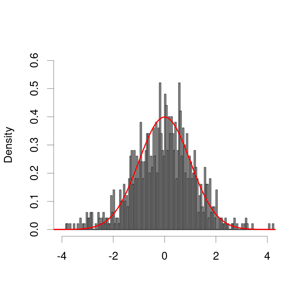
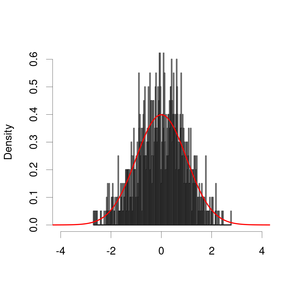
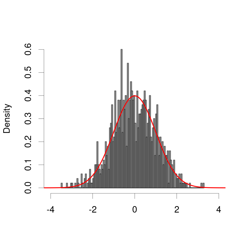
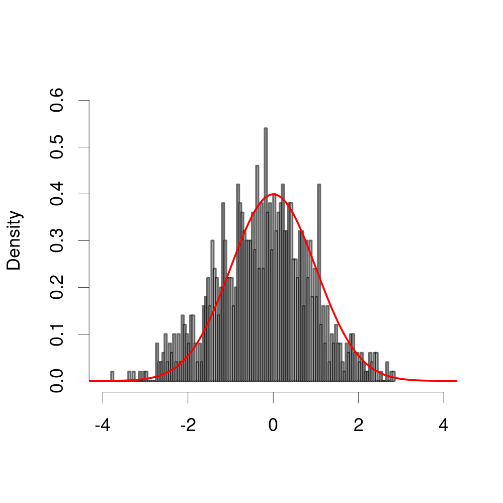
In the last experiment, we verify the asymptotic distributions of the smoothly estimated factor loadings in Theorem 5.2. To simplify the calculation of the asymptotic variances, we set in (10) and generate from i.i.d. . Figure 1 plots the empirical density of after standardization according to Theorem 5.2, over 1000 replications with or when the entries of are i.i.d. from , or . Under such cases, the asymptotic variance of is , where is the density of idiosyncratic error at after translation so that . Figure 1 clearly shows the asymptotic normality of the estimators with well fitted variances.


7 Real Data Analysis
7.1 Data description
In this section, we apply the proposed matrix quantile factor model and associated estimators to the analysis of a real data set, the Fama-French 100 portfolios data set. This an open resource provided by Kenneth R. French, which can be downloaded from the website http://mba.tuck.dartmouth.edu/pages/faculty/ken.french/data_library.html. It contains monthly return series of 100 portfolios, structured into a matrix according to 10 levels of market capital size (S1-S10) and 10 levels of book-to-equity ratio (BE1-BE10). Considering the missing rate, we use the data from 1964-01 to 2021-12 in this study, covering 696 months. Similar data set has ever been studied in Wang et al. (2019) and Yu et al. (2022). The data library also provides information on Fama-French three factors and excess market returns. Following the preprocessing steps in Wang et al. (2019) and Yu et al. (2022), we first subtract the excess market returns and standardize each of the portfolio return series.
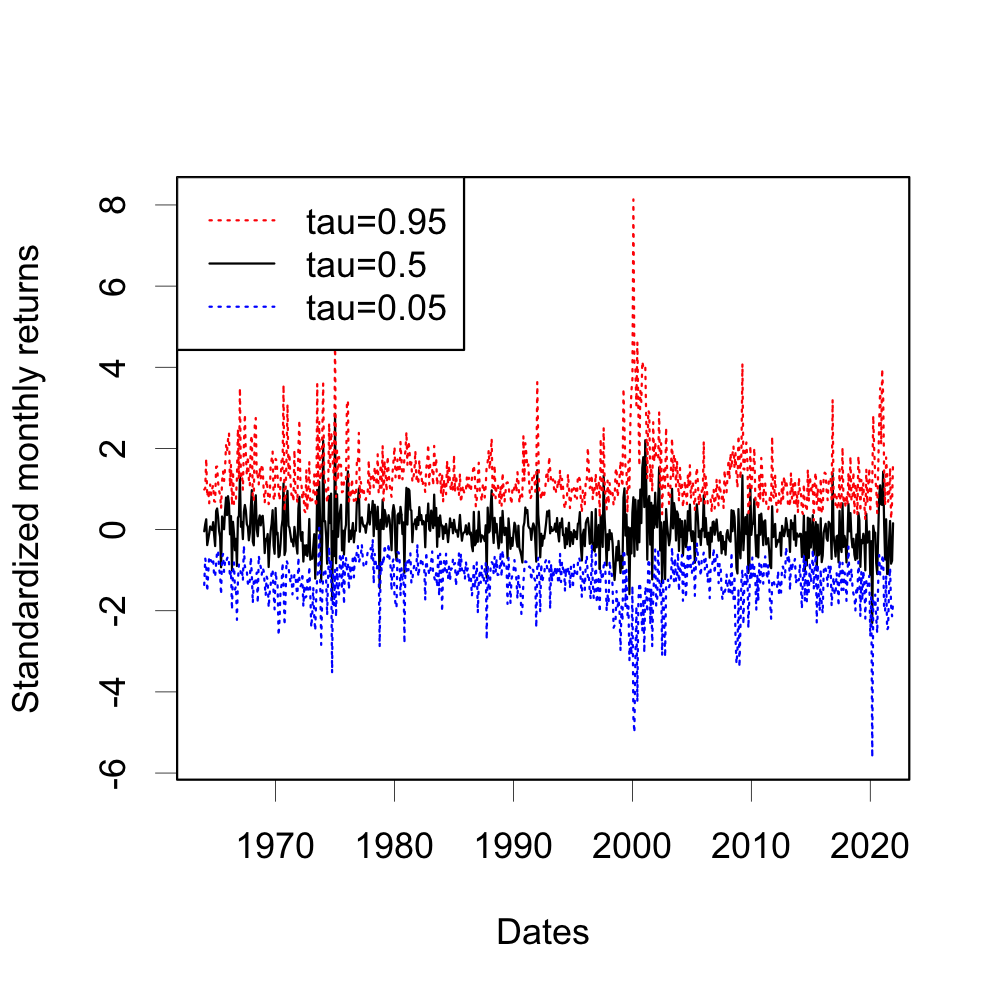
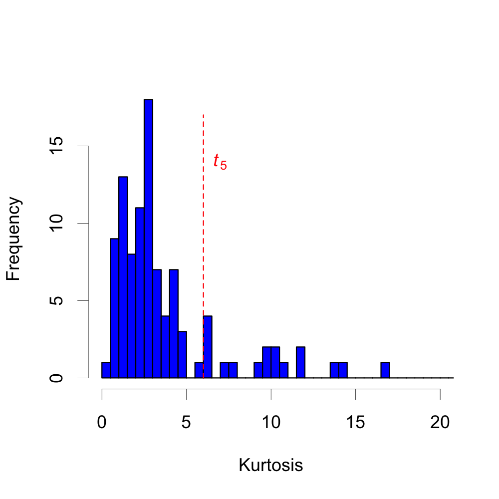
In the first step, we provide some descriptive information of the data set. At each month , we calculate sample quantiles of the 100 portfolios returns. Figure 3 plots the quantile series at . It’s seen that different quantile series contain disparate local patterns across the sampling periods. For instance, around the year 2000, the quantile series and the median series undergo a great increment while the quantile series drops significantly. That is to say, considering multiple quantiles will help in understanding the distribution of data. On the other hand, some extreme values are seen in the and quantile series, such as in mid-1970s, the years 2000, 2008 and 2020, which may indicate heavy-tailed property. The histogram in Figure 3 summarizes the total number of portfolio series associated with specific sample kurtosis. There are 18 portfolio series having sample kurtosis larger than the theoretical kurtosis of distribution, which is a convincing signal of heavy-tailed characteristic. According to our simulation results, it’s better to use the quantile factor model under such scenarios.
7.2 Estimation
In the second step, we fit the matrix quantile factor model. The numbers of row and column factors should be determined first. Table 7 provides the estimated using the proposed three approaches at different quantiles . The results by the vectorized method with Chen et al. (2021) are also reported in the table, which leads to the estimation of total number of factors. By Table 7, the proposed eigenvalue ratio method and information criterion always lead to an estimate of , while the rank minimization approach gives more row and/or column factors when . The vectorized method leads to an estimate of 2 factors in total at most quantiles. Based on the results, there should be at least one powerful row factor and column factor in the system, and potentially one weak row factor and/or column factor. When is at the edge, the leading factor becomes more influential. On the other hand, the approaches in Wang et al. (2019) and Yu et al. (2022) will both lead to . In this example, it might be a good choice to use when is around , and when is at the edge.
| Similarity of loading spaces | ||||||||
|---|---|---|---|---|---|---|---|---|
| mqf-ER | mqf-RM | mqf-IC | vqf-RM | |||||
| 0.05 | (1,1) | (1,1) | (1,1) | 1 | 0.503 | 0.661 | 0.381 | 0.691 |
| 0.1 | (1,1) | (1,1) | (1,1) | 1 | 0.965 | 0.914 | 0.736 | 0.725 |
| 0.15 | (1,1) | (1,2) | (1,1) | 2 | 0.992 | 0.961 | 0.723 | 0.719 |
| 0.2 | (1,1) | (2,1) | (1,1) | 2 | 0.991 | 0.957 | 0.724 | 0.716 |
| 0.25 | (1,1) | (2,2) | (1,1) | 2 | 0.998 | 0.979 | 0.737 | 0.726 |
| 0.3 | (1,1) | (2,2) | (1,1) | 2 | 0.996 | 0.991 | 0.747 | 0.744 |
| 0.35 | (1,1) | (2,2) | (1,1) | 2 | 0.997 | 0.996 | 0.738 | 0.737 |
| 0.4 | (1,1) | (2,2) | (1,1) | 2 | 0.998 | 0.996 | 0.722 | 0.723 |
| 0.45 | (1,1) | (2,2) | (1,1) | 2 | 0.997 | 0.992 | 0.707 | 0.702 |
| 0.5 | (1,1) | (2,2) | (1,1) | 2 | 0.999 | 0.993 | 0.674 | 0.666 |
| 0.55 | (1,1) | (2,2) | (1,1) | 2 | 0.988 | 0.996 | 0.673 | 0.659 |
| 0.6 | (1,1) | (2,2) | (1,1) | 2 | 0.993 | 0.997 | 0.674 | 0.676 |
| 0.65 | (1,1) | (2,2) | (1,1) | 2 | 0.989 | 0.998 | 0.705 | 0.703 |
| 0.7 | (1,1) | (2,2) | (1,1) | 2 | 0.990 | 0.994 | 0.740 | 0.737 |
| 0.75 | (1,1) | (2,2) | (1,1) | 2 | 0.975 | 0.982 | 0.727 | 0.716 |
| 0.8 | (1,1) | (1,2) | (1,1) | 2 | 0.977 | 0.924 | 0.743 | 0.727 |
| 0.85 | (1,1) | (1,2) | (1,1) | 2 | 0.958 | 0.967 | 0.723 | 0.703 |
| 0.9 | (1,1) | (2,2) | (1,1) | 1 | 0.985 | 0.937 | 0.711 | 0.699 |
| 0.95 | (1,1) | (1,1) | (1,1) | 1 | 0.884 | 0.873 | 0.607 | 0.627 |
The next step is to estimate the loading matrices and factor scores with . It’s worth noting that the quantile factor models can handle missing values naturally by optimization only with non-missing entries, i.e., by defining
where indicates the index set of all non-missing entries. However, the -PCA and “PE” methods require to impute the missing entries first. Considering that the missing rate is small in this example (), we use simple linear interpolation method to impute missing data. To measure the similarity of two estimated loading spaces, we define the following indicator:
where and are the estimated row loading matrices. Note that the columns of and are orthogonal after scaling. Therefore, the value is actually the projection matrix of to the space of . The value of will always be in the interval . When the two loading spaces are closer to each other, the value of will be larger.
The last four columns of Table 7 report the similarity of estimated loading spaces by matrix-quantile-factor-model and two competitors, “PE” and the vectorization approach. For the vectorization, we calculate similarity by considering the Kronecker product . It’s seen that the similarity indicators for the matrix-quantile-factor based approach and “PE” approach are very close to 1, implying that the estimated loading spaces are almost the same, especially when is near 0.5. However, when is at the edge, the difference of the estimated loading spaces becomes more significantly. For the vectorization approach, the estimated loading space is always not similar to that from the matrix models, consistent with our findings from the simulation study.
7.3 Interpretation
Now we aim to interpret the matrix quantile factors in this example. Table 8 presents the estimated and by matrix quantile factor model at , , as well as those by “PE‘”. By Table 8, the effects of the row factors and column factors are closely related to market capital sizes and book-to-equity ratios. From the perspective of size (), under the matrix quantile factor model with , the small-size portfolios load more heavily on the first factor than the large-size portfolios. Moreover, the second factor has opposite effects on small-size portfolios and large-size ones. Similar results are found for the “ PE” method, although the values of loadings are not exactly the same. Taking at edge will lead to different finding, where the first factor has more significant effect on the large-size portfolios. In other words, the edge quantile factors show disparate information of the data.
From the perspective of book-to-equity ratio (), with , the large-BE portfolios load more heavily on the first factor than small-BE ones, while the second factor has opposite effects on the two classes. The “PE” factors show similar trend after orthogonal transformation (changing sign). When and , the first factor depends on the average of all portfolios. It’s worth noting that the reported row and column factors are highly suggestive, because they coincide with financial theories. The capital size and book-to-equity ratio are known to be two important factors affecting portfolio returns in negative collaboration. The row and column factors in this example might be closely related to the SMB and HML factors in portfolio theory.
| Size () | |||||||||||
|---|---|---|---|---|---|---|---|---|---|---|---|
| Methods | Factors | S1 | S2 | S3 | S4 | S5 | S6 | S7 | S8 | S9 | S10 |
| 1 | 1.15 | 1.20 | 1.25 | 1.21 | 1.14 | 1.08 | 0.90 | 0.78 | 0.55 | 0.00 | |
| 2 | 1.28 | 0.83 | 0.53 | 0.23 | -0.22 | -0.57 | -0.86 | -1.11 | -1.66 | -1.49 | |
| PE | 1 | -1.17 | -1.21 | -1.26 | -1.20 | -1.15 | -1.04 | -0.90 | -0.81 | -0.54 | 0.01 |
| 2 | 1.39 | 0.95 | 0.48 | 0.18 | -0.28 | -0.65 | -0.91 | -1.18 | -1.56 | -1.31 | |
| 1 | 0.81 | 0.87 | 0.85 | 0.99 | 1.02 | 1.07 | 1.03 | 1.05 | 1.12 | 1.14 | |
| 2 | 1.04 | 1.30 | 1.42 | 0.66 | 0.68 | -0.18 | -0.54 | -0.85 | -1.30 | -1.25 | |
| 1 | 0.83 | 0.84 | 0.86 | 0.87 | 0.97 | 1.04 | 1.03 | 1.05 | 1.15 | 1.28 | |
| 2 | -0.63 | 0.15 | 0.71 | 0.51 | 0.04 | 0.83 | -0.82 | -0.83 | -1.87 | 1.81 | |
| Book-to-Equity () | |||||||||||
| Methods | Factors | BE1 | BE2 | BE3 | BE4 | BE5 | BE6 | BE7 | BE8 | BE9 | BE10 |
| 1 | 0.59 | 0.74 | 0.95 | 1.05 | 1.12 | 1.16 | 1.12 | 1.13 | 1.08 | 0.89 | |
| 2 | 2.13 | 1.67 | 0.75 | 0.29 | -0.07 | -0.58 | -0.68 | -0.73 | -0.67 | -0.52 | |
| PE | 1 | -0.53 | -0.83 | -1.01 | -1.08 | -1.10 | -1.12 | -1.12 | -1.08 | -1.07 | -0.90 |
| 2 | 2.16 | 1.56 | 0.81 | 0.31 | -0.15 | -0.50 | -0.69 | -0.77 | -0.70 | -0.55 | |
| 1 | 0.98 | 0.90 | 0.94 | 1.09 | 1.11 | 1.07 | 0.96 | 1.03 | 0.86 | 1.05 | |
| 2 | 1.33 | 1.37 | 1.20 | 0.61 | 0.08 | -0.55 | -0.81 | -1.04 | -1.40 | -0.74 | |
| 1 | 0.99 | 1.02 | 1.01 | 1.00 | 1.00 | 1.01 | 0.99 | 1.00 | 0.99 | 0.98 | |
| 2 | -1.61 | 0.39 | 1.84 | -0.17 | -0.09 | -1.44 | 0.00 | 0.26 | -0.42 | 1.23 | |
7.4 Robustness to outliers
One of our motivation to consider matrix quantile factor model is the robustness of the check losss function. In this part, We verify it with this real example. We manually corrupt a small proportion of the data with (randomly), and re-estimate the factor loadings. We compare the robustness of the estimators using , where “new” and “old”‘ indicate after and before corruption, respectively. To reduce the randomness in the corruption step, we repeat the process 50 times and report the average similarity in Figure 4, with various corruption proportion.
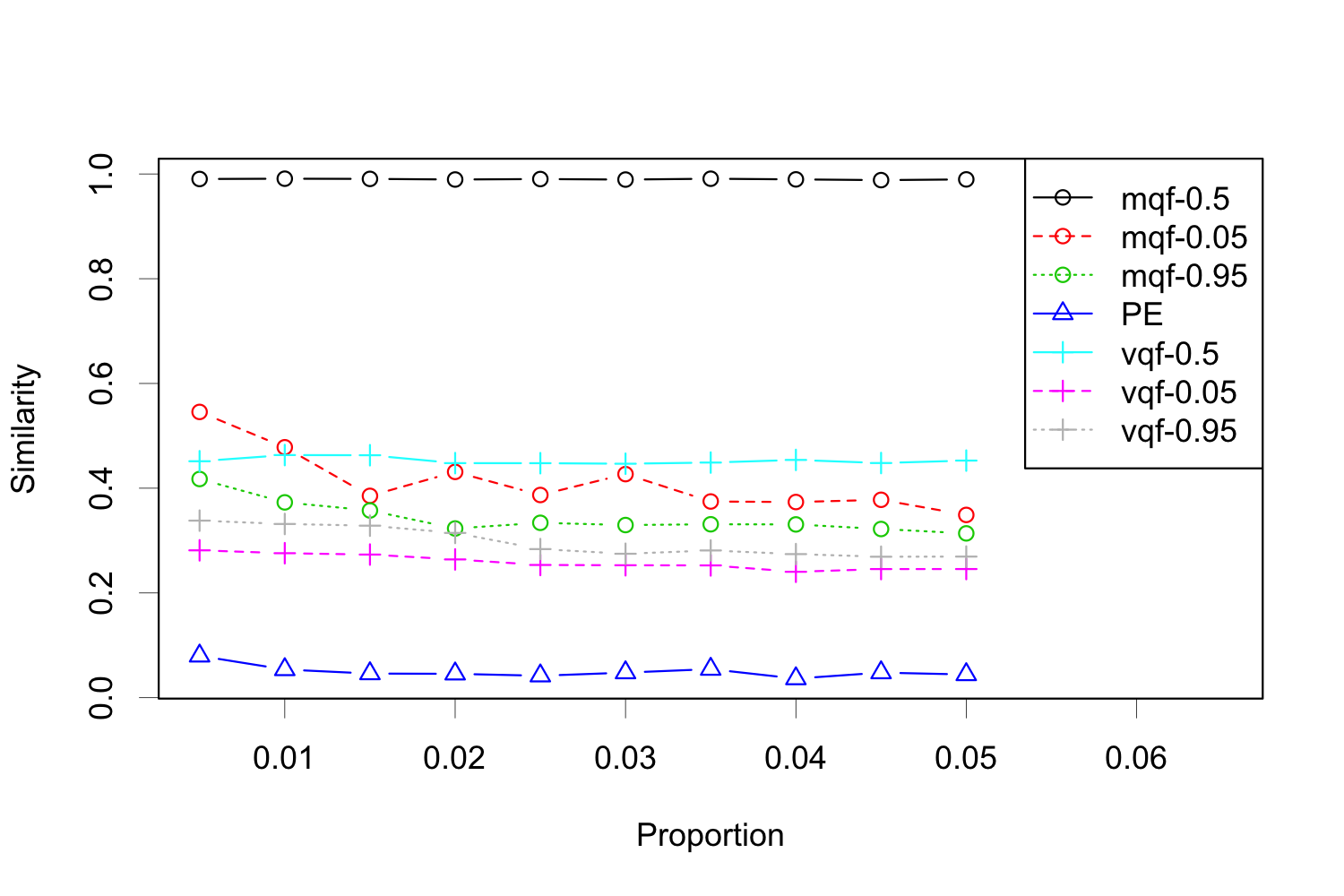
By Figure 4, the matrix quantile factor model with is the most robust, as expected. There is no significant change of the loading space even if the corruption rate is as large as . The model with seems to be more stable compared with the case in this example, potentially because the data is not symmetric. The “PE” method is very sensitive to the outliers, and the loading matrix almost moves to its orthogonal complementary space after corruption. The stability of the vectorization approach lies between that of the matrix quantile model and the “PE” method.
7.5 Usefulness in prediction
By Table 7, when is at the edge, the similarity indicator decreases, suggesting that considering the edge quantiles might be helpful for extracting extra information from the data. However, by Figure 4, the low similarity can also potentially results from the reduced stability. Therefore, to justify the usefulness of the proposed model, we construct a rolling prediction procedure as follows. Let be any of the Fama-French three factors at month . We consider a forecasting model for :
where is a vector of estimated factors from the Fama-French 100 portfolio data set. We estimate using ordinary least squares. For , we consider eight specifications: (i) , which is the benchmark AR(1) model, (ii) from “PE”, (iii) from “PE” and matrix quantile factor model at , (iv) from “PE” and matrix quantile factor model at , (v) from “PE” and matrix quantile factor model at and , (vi) to (viii) generate similarly to (iii) to (v) but replacing matrix quantile factors with vectorized quantile factors. To control the dimension of the design matrix, we use in this part, and ignore the case because the estimated loading space is very close to that from “PE” by Table 7. To predict , we first estimate all the factors using historical data before (inclusive) with a rolling window of 60 months, and then fit the predicting model using data only before . The predictor then follows the fitted model. Table 9 reports the root of mean squared error (RMSE) and mean absolute error (MAE) for the prediction over all the periods, from different predicting models and for different Fama-French factors. As shown in the table, adding estimated factors into the model helps reduce the error for the SMB factor and the HML factor, while considering the edge quantiles further improves the prediction performance. This is consistent with our interpretation in Section 7.3. The estimated row and column factors from the matrix quantile factor model are closely related to the Fama and French SMB and HML factors. In this example, the matrix quantile factor model leads to smaller MAE while the vectorized model leads to smaller RMSE. But for the RF factor, the Benchmark AR(1) model works already the best. Adding more factors into the predictors only results in more errors, mainly because the market excess return has already been removed from the data.
| SMB factor | HML factor | RF factor | ||||
| Predicting models | RMSE | MAE | RMSE | MAE | RMSE | MAE |
| AR benchmark | 3.182 | 2.272 | 3.020 | 2.185 | 0.065 | 0.040 |
| AR plus | 1.692 | 1.101 | 2.953 | 2.180 | 0.065 | 0.041 |
| AR plus , | 1.610 | 1.058 | 3.045 | 2.199 | 0.066 | 0.041 |
| AR plus , | 1.563 | 1.032 | 2.975 | 2.190 | 0.065 | 0.042 |
| AR plus , , | 1.441 | 0.924 | 2.824 | 2.057 | 0.067 | 0.042 |
| AR plus , | 1.624 | 1.063 | 3.019 | 2.195 | 0.066 | 0.041 |
| AR plus , | 1.589 | 1.039 | 2.976 | 2.178 | 0.065 | 0.041 |
| AR plus , , | 1.429 | 0.932 | 2.815 | 2.069 | 0.066 | 0.042 |
7.6 Usefulness in imputing missing values
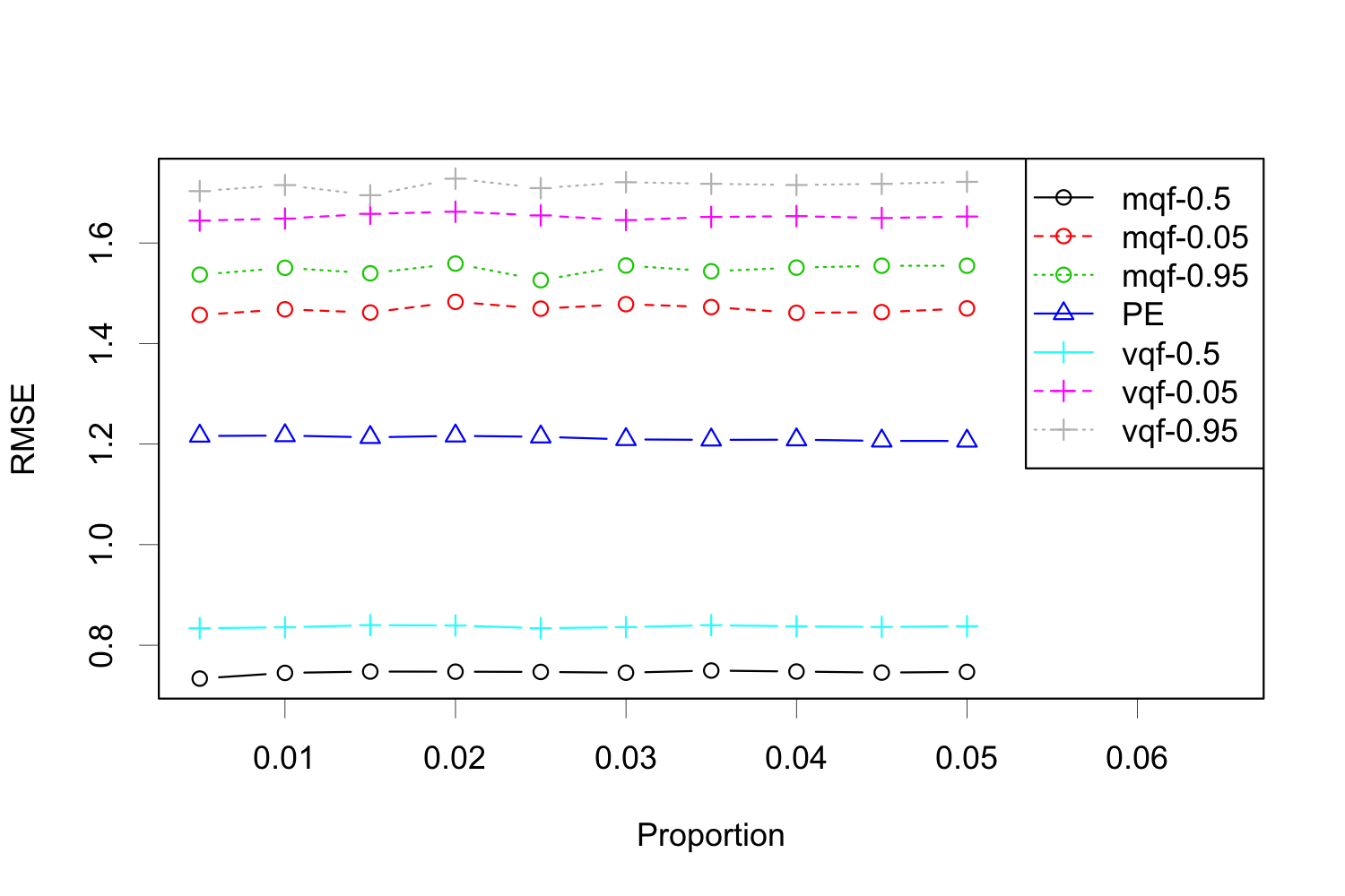
In our last experiment, we investigate the performance of matrix quantile factor model in imputing missing entries. We deliberately kick out a proportion of entries from the data, and treat them as missing values. Then, we fit a factor model, estimate the loading and factor score matrices, and impute the missing entries by the estimated common components. We calculate the imputing error in terms of RMSE, denoted by . As a benchmark, we also calculate the imputing error when simply imputing the missing values with 0 (the data are standardized), denoted as . For robustness check, we repeat the procedure 50 times and report the averaging under different factor models in Figure 5, as the kicking-out proportion increases. It’s seen that the matrix-quantile factor model with leads to the lowest imputing error in all scenarios.
8 Conclusion and Discussion
In this study, we proposed a matrix quantile factor model that is a hybrid of quantile feature representation and a low rank structure for matrix data. By minimizing the check loss function with an iterative algorithm, we obtain estimates of the row and column factor spaces that are proved to be consistent in the sense of Frobenious norm. Three model selection criteria were given to consistently determine simultaneously the numbers of row and column factors. Central limit theorems are derived for the smoothed loading estimates. There are at least three problems that are worthy of being studied in the future. First, a statistical test for the presence of the low-rank matrix structure in the matrix quantile factor model is of potential usefulness as a model checking tool. Second, the latent factor structure here can be extended to the case where both observable explanatory variables and latent factors are incorporated into modeling the quantiles of matrix sequences. Third, the computation error with the algorithm, that parallels to the statistical error given in our theorem, is still unknown. We leave all these to our future research work.
9 Supplementary Material
The technical proofs of the main results are included in the supplementary material.
References
- Aanæs et al. (2002) Aanæs, H., R. Fisker, K. Åström, and J. M. Carstensen (2002). Robust factorization. IEEE Transactions on Pattern Analysis and Machine Intelligence 24(9), 1215–1225.
- Ahn and Horenstein (2013) Ahn, S. C. and A. R. Horenstein (2013). Eigenvalue ratio test for the number of factors. Econometrica 81(3), 1203–1227.
- Aït-Sahalia and Xiu (2017) Aït-Sahalia, Y. and D. Xiu (2017). Using principal component analysis to estimate a high dimensional factor model with high-frequency data. Journal of Econometrics 201, 384–399.
- Ando and Bai (2021) Ando, T. and J. Bai (2021). Quantile co-movement in financial markets: A panel quantile model with unobserved heterogeneity. Journal of the American Statistical Association 115(529), 266–279.
- Ando et al. (2019) Ando, T., J. Bai, M. Nishimura, and J. Yu (2019). A Quantile-based Asset Pricing Model. Economics and Statistics Working Papers (15-2019).
- Bai (2003) Bai, J. (2003). Inferential theory for factor models of large dimensions. Econometrica 71(1), 135–171.
- Bai and Ng (2002) Bai, J. and S. Ng (2002). Determining the number of factors in approximate factor models. Econometrica 70(1), 191–221.
- Barigozzi and Trapani (2020) Barigozzi, M. and L. Trapani (2020). Sequential testing for structural stability in approximate factor models. Stochastic Processes and their Applications 130(8), 5149–5187.
- Chang et al. (2023) Chang, J., J. He, L. Yang, and Q. Yao (2023). Modelling matrix time series via a tensor CP-decomposition. Journal of the Royal Statistical Society: Series B (Statistical Methodology), to appear, doi: 10.1093/jrsssb/qkac011.
- Chen and Chen (2020) Chen, E. Y. and R. Chen (2020). Modeling dynamic transport network with matrix factor models: with an application to international trade flow. arXiv:1901.00769.
- Chen and Fan (2021) Chen, E. Y. and J. Fan (2021). Statistical inference for high-dimensional matrix-variate factor models. Journal of the American Statistical Association, In Press, https://doi.org/10.1080/01621459.2021.1970569.
- Chen et al. (2020) Chen, E. Y., R. S. Tsay, and R. Chen (2020). Constrained factor models for high-dimensional matrix-variate time series. Journal of the American Statistical Association 115(530), 775–793.
- Chen et al. (2021) Chen, L., J. J. Dolado, and J. Gonzalo (2021). Quantile factor models. Econometrica 89(2), 875–910.
- Chen et al. (2022) Chen, R., D. Yang, and C.-H. Zhang (2022). Factor models for high-dimensional tensor time series. Journal of the American Statistical Association 117(537), 94–116.
- Chen et al. (2023) Chen, X., D. Yang, Y. Xu, Y. Xia, D. Wang, and H. Shen (2023). Testing and support recovery of correlation structures for matrix-valued observations with an application to stock market data. Journal of Econometrics 232(2), 544–564.
- Fan et al. (2013) Fan, J., Y. Liao, and M. Mincheva (2013). Large covariance estimation by thresholding principal orthogonal complements. Journal of the Royal Statistical Society: Series B (Statistical Methodology) 75(4), 603–680.
- Gao et al. (2021) Gao, Z., C. Yuan, B. Jing, H. Wei, and J. Guo (2021). A two-way factor model for high-dimensional matrix data. arXiv:2103.07920.
- Ge et al. (2017) Ge, R., C. Jin, and Y. Zheng (2017). No spurious local minima in nonconvex low rank problems: A unified geometric analysis. Proceedings of the 34th International Conference on Machine Learning PMLR 70, 1233–1242.
- Han et al. (2021) Han, Y., C.-H. Zhang, and R. Chen (2021). CP factor model for dynamic tensors. arXiv preprint arXiv:2110.15517.
- He et al. (2022) He, Y., X. Kong, L. Yu, and X. Zhang (2022). Large-dimensional factor analysis without moment constraints. Journal of Business & Economic Statistics 40(1), 302–312.
- He et al. (2023) He, Y., X. Kong, L. Yu, and P. Zhao (2023). Quantile factor analysis for large-dimensional time series with statistical guarantee. arXiv preprint arXiv:2006.08214.
- Ke and Kanade (2005) Ke, Q. and T. Kanade (2005). Robust norm factorization in the presence of outliers and missing data by alternative convex programming. Proceedings of the 2005 IEEE computer society conference on computer vision and pattern recognition CVPR’05, 1063–1069.
- Kong (2017) Kong, X. (2017). On the number of common factors with high-frequency data. Biometrika 104(2), 397–410.
- Kong (2018) Kong, X. (2018). On the systematic and idiosyncratic volatility with large panel high-frequency data. The Annals of Statistics 46(3), 1077–1108.
- Kong et al. (2019) Kong, X., J. Wang, J. Xing, C. Xu, and C. Ying (2019). Factor and idiosyncratic empirical processes. Journal of the American Statistical Association 114(527), 1138–1146.
- Onatski (2010) Onatski, A. (2010). Determining the number of factors from empirical distribution of eigenvalues. Review of Economic Statistics 92(4), 1004–1016.
- Pelger (2019) Pelger, M. (2019). Large-dimensional factor modeling based on high-frequency observations. Journal of Econometrics 208, 23–42.
- Stock and Watson (2002a) Stock, J. H. and M. W. Watson (2002a). Forecasting using principal components from a large number of predictors. Journal of the American statistical association 97(460), 1167–1179.
- Stock and Watson (2002b) Stock, J. H. and M. W. Watson (2002b). Macroeconomic forecasting using diffusion indexes. Journal of Business & Economic Statistics 20(2), 147–162.
- Trapani (2018) Trapani, L. (2018). A randomised sequential procedure to determine the number of factors. Journal of the American Statistical Association 113, 1341–1349.
- Van Loan (2000) Van Loan, C. (2000). The ubiquitous kronecker product. Journal of Computational and Applied mathematics 123(1), 85–100.
- Wang et al. (2019) Wang, D., X. Liu, and R. Chen (2019). Factor models for matrix-valued high-dimensional time series. Journal of Econometrics 208(1), 231–248.
- Yu et al. (2022) Yu, L., Y. He, X. Kong, and X. Zhang (2022). Projected estimation for large-dimensional matrix factor models. Journal of Econometrics 229, 201–217.
- Zhang et al. (2022) Zhang, X., G. Li, and C. C. Liu (2022). Tucker tensor factor models for high-dimensional higher-order tensor observations. arXiv preprint arXiv:2206.02508.