Small Tuning Parameter Selection for the Debiased Lasso

Abstract

In this study, we investigate the bias and variance properties of the debiased Lasso in linear regression when the tuning parameter of the node-wise Lasso is selected to be smaller than in previous studies. We consider the case where the number of covariates $p$ is bounded by a constant multiple of the sample size $n$. First, we show that the bias of the debiased Lasso can be reduced without diverging the asymptotic variance by setting the order of the tuning parameter to $1/\sqrt{n}$. This implies that the debiased Lasso has asymptotic normality provided that the number of nonzero coefficients $s_{0}$ satisfies $s_{0}=o(\sqrt{n/\log p})$, whereas previous studies require $s_{0}=o(\sqrt{n}/\log p)$ if no sparsity assumption is imposed on the precision matrix. Second, we propose a data-driven tuning parameter selection procedure for the node-wise Lasso that is consistent with our theoretical results. Simulation studies show that our procedure yields confidence intervals with good coverage properties in various settings. We also present a real economic data example to demonstrate the efficacy of our selection procedure.

Keywords: Lasso, debiasing, high-dimensional data, confidence intervals, hypothesis testing.

1 Introduction

In this study, we make inferences about individual coefficients of the linear regression model:

$$Y=X\beta_{0}+\epsilon,$$ (1)

where $Y\in\mathbb{R}^{n}$ denotes the response, $X=(X_{1},\dots,X_{p})\in\mathbb{R}^{n\times p}$ denotes the random design matrix, $\beta_{0}\in\mathbb{R}^{p}$ denotes the unknown regression coefficient, and $\epsilon\in\mathbb{R}^{n}\sim N(0,\sigma_{\epsilon}^{2}I)$ denotes the unobservable noise that is independent of $X$. We consider $p>n$ and assume that $X$ has zero mean and a positive definite covariance matrix $\Sigma=E[X^{T}X/n]$. We focus on statistical inferences for $\beta_{01}$, the first component of $\beta_{0}$, although the inferences are equally valid for other components.

Much research has been conducted on high-dimensional linear regression models. The Lasso (Tibshirani, 1996) is one of the most popular methods for estimating their coefficients. The popularity is due to variable selection properties, the oracle inequalities (Bickel et al., 2009, Bühlmann and van de Geer, 2011), and useful computational algorithms (Efron et al., 2004, Friedman et al., 2010). Bühlmann and van de Geer, (2011) gave excellent overviews of the Lasso. However, the asymptotic distribution of the Lasso is generally intractable because the Lasso is biased and the distribution is not continuous (Knight and Fu, 2000). Therefore, it is difficult to perform statistical inference based on the Lasso itself, and there are currently three main approaches of performing statistical inference in high-dimensional linear regression models.

The first approach of inference is the so-called selective inference. See Berk et al., (2013), Lee et al., (2016), Tibshirani et al., (2016), and Tibshirani et al., (2018), among others. Statistical inferences after model selection are distorted if the selected model is treated as if it is a true one. Rather than making inferences on coefficients of the true regression model, the selective inference makes inferences on coefficients in a model selected via data-driven procedures. The validity of the inferences does not depend on the correctness of the selected model.

The second approach is the orthogonalization approach, which is developed in econometrics. Some contributions include the post-double selection method of Belloni et al., (2014), projection onto the double selection method of Wang et al., (2020), and double machine learning method of Chernozhukov et al., (2018). Such methods perform inference on low-dimensional parameters when high-dimensional nuisance parameters appear in regression models. The estimators of the parameter of interest are derived through the orthogonal score function, which is insensitive to the estimation of nuisance parameters.

The third approach is to debias or desparsify the Lasso, which we consider in this study. The debiased Lasso was proposed by Zhang and Zhang, (2014) and further developed by van de Geer et al., (2014) and Javanmard and Montanari, (2014). Unlike selective inference, this approach is intended to make inferences on coefficients in the true linear regression model. If the true data generating process is sufficiently sparse, the estimator is asymptotically normally distributed, so that inference is possible even when $p>n$.

The performance of the debiased Lasso depends on the degree of sparsity and the choice of tuning parameters. To obtain the debiased Lasso estimator of $\beta_{01}$, we need an estimate of $\Theta_{1}$, the first column of $\Sigma^{-1}$, and the node-wise Lasso (Meinshausen and Bühlmann, 2006) is commonly used to obtain it. Therefore, the debiased Lasso estimator depends on the tuning parameters of the Lasso $\lambda_{0}$ and node-wise Lasso $\lambda_{1}$. Let $s_{0}$ and $s_{1}$ be the numbers of nonzero components in $\beta_{0}$ and $\Theta_{1}$, respectively. If both $\lambda_{0}$ and $\lambda_{1}$ are of order $\sqrt{\log p/n}$, the asymptotic normality of the debiased Lasso is shown for $s_{0}=o(\sqrt{n}/\log p)$ and $s_{1}=o(n/\log p)$ (van de Geer et al., 2014, Zhang and Zhang, 2014) or for $s_{0}=o(n/\|\Theta_{1}\|_{1}^{2}(\log p)^{2})$ and $\min\{s_{0},s_{1}\}=o(\sqrt{n}/\log p)$ (Javanmard and Montanari, 2018). Recently, Bellec and Zhang, (2022) showed asymptotic normality of the debiased Lasso when $\max\{s_{0},s_{1}\}=o(n/\log p)$ and $\min\{s_{0},s_{1}\}=o(\sqrt{n}/\log p)$ using degrees of freedom adjustments.

Although the above studies significantly contributed to the development of the debiased Lasso, there are two main issues to be addressed. First, the bias of the debiased Lasso may not be asymptotically negligible if $\Theta_{1}$ and $\beta_{0}$ are not sufficiently sparse. If no sparsity condition is imposed on $\Theta_{1}$, $s_{0}$ must satisfy $s_{0}=o(\sqrt{n}/\log p)$ for zero-mean asymptotic normality, which is rather restrictive given that only $s_{0}=o(n/\log p)$ is need for consistent estimation. Second, existing tuning parameter selection procedures of $\lambda_{1}$, such as the cross-validation (Chetverikov et al., 2021) and the methods of Zhang and Zhang, (2014) and Dezeure et al., (2015), often produce a rather large bias in the debiased Lasso, yielding a poor coverage of confidence intervals and large size distortion of $t$ tests.

We address these two issues by selecting a smaller tuning parameter of the node-wise Lasso than in prior studies. First, we show that by setting the order of $\lambda_{1}$ to $1/\sqrt{n}$, the bias of the debiased Lasso can be reduced without diverging the asymptotic variance, so that asymptotic normality holds provided $s_{0}=o(\sqrt{n/\log p})$. The novelty of our method is that we intentionally overfit the node-wise Lasso to reduce the bias of the debiased Lasso. Further, our analysis does not impose any sparsity assumption on $\Theta_{1}$. To the best of our knowledge, there is no asymptotic normality result of the debiased Lasso when the order of $\lambda_{1}$ is $1/\sqrt{n}$. Moreover, with the exception of van de Geer, (2019), no prior study, including Belloni et al., (2014) and Chernozhukov et al., (2018), has established asymptotic normality without imposing any sparsity condition on $\Theta_{1}$. A sufficient condition for our result is that each row vector of $X$ is independent Gaussian and $p\leq Cn$ for some $C<\infty$. Although the condition that $p$ and $n$ be of the same order excludes some high-dimensional data, such as genomic data, various data fit the condition in many fields, such as economics.

Second, we propose a data-driven procedure to select $\lambda_{1}$, which we call the small tuning parameter selector (STPS). We modify the selection method of Zhang and Zhang, (2014) so that the selector chooses a tuning parameter with a reasonably small value. Figure 1 compares the distributions of the debiased Lasso whose $\lambda_{1}$ is selected by cross-validation and STPS, respectively, indicating that STPS successfully reduces the bias. Simulation studies show that the debiased Lasso tuned by our procedure outperforms other inference methods, such as the double machine learning, post-double selection, and debiased Lasso with other tuning parameter selection methods. This is particularly true when $\beta_{0}$ and $\Theta_{1}$ are dense. We also show a real economic data example to see the performance of our method. Because the true sparsity of $\beta_{0}$ and $\Theta_{1}$ is unknown, it is essential to propose a selection method that is robust to the violation of the sparsity condition.

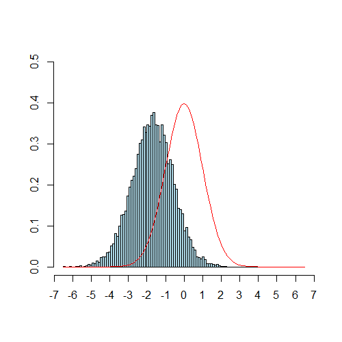
(a) 10-fold cross-validation.

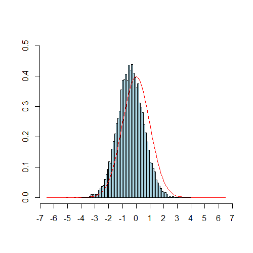
(b) STPS.

Figure 1: Distributions of the studentized debiased Lasso (histogram) and the standard normal distribution (solid line). We employ the simulation design II of Table II in Kozbur, (2020) with $n=200$ and $p=400$ and repeat experiments 10,000 times. The tuning parameter $\lambda_{0}$ of the Lasso to be debiased is selected by the 10-fold cross-validation. The error variance is estimated by the sample mean of squared residuals from the Lasso tuned by the one standard error rule. For panel (a), the 10-fold cross-validation selects $0.13$ on average, and the coverage of 95% confidence interval is 59.7% with the average length of 0.208. For panel (b), STPS selects $0.001$ on average, and the coverage of 95% confidence interval is 94.3% with the average length of 0.459.

We emphasize that the aim of this study is not to obtain an asymptotically efficient estimator (see, e.g., van de Geer et al., 2014, Jankova and van de Geer, 2018, van de Geer, 2019, and Bellec and Zhang, 2022 about the asymptotic efficiency of the debiased Lasso). The aim is to construct confidence intervals with good coverage properties or test statistics with the correct size. There is a bias–variance tradeoff with respect to $\lambda_{1}$. Our method reduces the bias at the cost of slightly increasing the variance. Setting the order of $\lambda_{1}$ to $1/\sqrt{n}$ maintains the $\sqrt{n}$-consistency of the debiased Lasso, although the asymptotic variance may exceed the efficiency bound.

The remainder of this article is organized as follows. In Section 2, we formally state an asymptotic normality result of the debiased Lasso when the order of $\lambda_{1}$ is $1/\sqrt{n}$. In Section 3, we propose a data-driven method to select $\lambda_{1}$. In Section 4, we show results of extensive simulation studies for the debiased Lasso tuned by our procedure and other statistical inference methods. We present a real economic data example based on the considered methods in Section 5. Finally, concluding remarks are presented in Section 6. All proofs are given in Appendix.

2 Theoretical Results

We define $|S|$ as the cardinality of a set $S$. Let $a^{T}$ be the transpose of a vector $a$. Let $\|a\|$, $\|a\|_{1}$, and $\|a\|_{\infty}$ be the Euclidean norm, $\ell_{1}$ norm, and maximum element in the absolute value of a vector $a$, respectively. For any sequences of real numbers $\{a_{n}\}$ and $\{b_{n}\}$, $a_{n}\asymp b_{n}$ means $C_{1}\leq a_{n}/b_{n}\leq C_{2}$ for all $n$ and some $C_{1},C_{2}>0$. Let $a_{n}\ll b_{n}$ and $b_{n}\gg a_{n}$ denote $\lim_{n\rightarrow\infty}|a_{n}/b_{n}|=0$. Let $a_{n}\lesssim b_{n}$ and $b_{n}\gtrsim a_{n}$ denote $a_{n}\leq Cb_{n}$ for all $n$ and some $C>0$. Let us denote $\lambda_{\min}(A)$ and $\lambda_{\max}(A)$ as the minimum and maximum eigenvalues for a matrix $A$, respectively.

2.1 Bias of the Debiased Lasso

First, we introduce the debiased Lasso. The Lasso for $\beta_{0}$ is defined as follows:

$$\hat{\beta}:=\mathop{\rm argmin}\limits_{\beta\in\mathbb{R}^{p}}\frac{1}{n}\|Y-X\beta\|^{2}+2\lambda_{0}\|\beta\|_{1},$$ (2)

where $\lambda_{0}>0$ denotes the tuning parameter. The debiased Lasso $\hat{b}_{1}$ for $\beta_{01}$ is given by

$$\hat{b}_{1}=\hat{\beta}_{1}+\frac{1}{n}\hat{\Theta}_{1}{\!\!}^{T}X^{T}(Y-X\hat{\beta}),$$ (3)

where $\hat{\beta}_{1}$ denotes the first component of $\hat{\beta}$, and $\hat{\Theta}_{1}$ denotes an estimate of $\Theta_{1}$.

Although it is not a requisite, $\hat{\Theta}_{1}$ is commonly constructed by the node-wise Lasso. Let $X_{-1}$ be a submatrix of $X$ without $X_{1}$. We define

$$\hat{\gamma}_{1}:=\mathop{\rm argmin}\limits_{\gamma\in\mathbb{R}^{p-1}}\frac{1}{n}\|X_{1}-X_{-1}\gamma\|^{2}+2\lambda_{1}\|\gamma\|_{1},$$

where $\lambda_{1}>0$ is another tuning parameter. Let $\tau_{1}^{2}$ denote the error variance in regressing $X_{1}$ on $X_{-1}$. Moreover, let us define $\tilde{\tau}_{1}^{2}$ and $\hat{\tau}_{1}^{2}$ as

$$\tilde{\tau}_{1}^{2}:=\frac{1}{n}\|X_{1}-X_{-1}\hat{\gamma}_{1}\|^{2},\ \ \hat{\tau}_{1}^{2}:=\tilde{\tau}_{1}^{2}+\lambda_{1}\|\hat{\gamma}_{1}\|_{1}.$$

The Karush-Kuhn–Tucker (KKT) conditions for the node-wise Lasso yield $\hat{\tau}_{1}^{2}=X_{1}^{T}(X_{1}-X_{-1}\hat{\gamma}_{1})/n$. Then, $\hat{\Theta}_{1}$ is given by

$$\hat{\Theta}_{1}:=\frac{1}{\hat{\tau}_{1}^{2}}(1,-\hat{\gamma}_{1}^{T})^{T}.$$

By a simple calculation, we get

$$\sqrt{n}(\hat{b}_{1}-\beta_{01})=\frac{1}{\sqrt{n}}\hat{\Theta}_{1}^{T}X^{T}\epsilon+\Delta_{1},$$ (4)

where

$$\Delta_{1}:=\sqrt{n}(\hat{\Sigma}\hat{\Theta}_{1}-e_{1})^{T}(\beta_{0}-\hat{\beta}),$$

and $e_{1}$ is the unit vector whose first element is unity.

From (4), the proof of asymptotic normality hinges on showing that the bias term $\Delta_{1}$ is asymptotically negligible. For $\min\{s_{0},s_{1}\}=o(\sqrt{n}/\log p)$, Javanmard and Montanari, (2018) and Bellec and Zhang, (2022) developed skillful techniques to evaluate the bias. Otherwise, it is common to rely on the $\ell_{1}$-$\ell_{\infty}$ Hölder inequality:

$$|\Delta_{1}|\leq\sqrt{n}\|\hat{\Sigma}\hat{\Theta}_{1}-e_{1}\|_{\infty}\|\hat{\beta}-\beta_{0}\|_{1}\leq\sqrt{n}\frac{\lambda_{1}}{\hat{\tau}_{1}^{2}}\|\hat{\beta}-\beta_{0}\|_{1}.$$ (5)

The last inequality in (5) is due to the KKT conditions for the node-wise Lasso. Under certain conditions, the Lasso satisfies $\|\hat{\beta}-\beta_{0}\|_{1}=O_{p}(s_{0}\sqrt{\log p/n})$ and the convergence rate cannot be improved. Thus, the order of the bias significantly depends on $\lambda_{1}/\hat{\tau}_{1}^{2}$. It has been shown that $\lambda_{1}/\hat{\tau}_{1}^{2}=O_{p}(\sqrt{\log p/n})$ for the choice of $\lambda_{1}\asymp\sqrt{\log p/n}$ in previous studies, such as van de Geer et al., (2014). They have shown that $1/\hat{\tau}_{1}^{2}=O_{p}(1)$ using the fact that $\hat{\gamma}_{1}$ converges to its population counterpart if $\lambda_{1}\asymp\sqrt{\log p/n}$ and $s_{1}=o(n/\log p)$.

In this study, we present a new evaluation method of the bias by showing that $1/\hat{\tau}_{1}^{2}=O_{p}(1)$ for $\lambda_{1}\asymp 1/\sqrt{n}$. Different from previous studies, we do not need consistency of the node-wise Lasso. Instead, we bound $1/\hat{\tau}_{1}^{2}$ using the properties of the node-wise Lasso derived from the general position assumption and conditions on the restricted eigenvalues of $\hat{\Sigma}$. This allows us not to restrict the sparsity of $\Theta_{1}$. A crucial point to bound $1/\hat{\tau}_{1}^{2}$ is bounding $1/\tilde{\tau}_{1}^{2}$, which is an upper bound of $1/\hat{\tau}_{1}^{2}$ and the variance factor of the debiased Lasso. Because Zhang and Zhang, (2014) showed that $1/\tilde{\tau}_{1}^{2}$ is a nonincreasing function in $\lambda_{1}$, selecting too small $\lambda_{1}$ may make $1/\tilde{\tau}_{1}^{2}$ and the variance diverge. We show that the debiased Lasso is $\sqrt{n}$-consistent even for $\lambda_{1}\asymp 1/\sqrt{n}$, although the asymptotic variance may be greater than when $\lambda_{1}\asymp\sqrt{\log p/n}$.

2.2 Asymptotic Normality with Small Tuning Parameter

To obtain the new bound for the bias, we first introduce four generic assumptions. Then, we show that the assumptions are satisfied under rather simple conditions. Roughly speaking, our assumptions are satisfied if $p$ is bounded by a constant multiple of $n$.

The first assumption is the general position assumption of Tibshirani, (2013).

Assumption 1.

For any $k<\min\{n,p\}$, the affine span of $\sigma_{1}X_{i_{1}},\ldots,\sigma_{k+1}X_{i_{k+1}}$ for arbitrary signs $\sigma_{1},\ldots,\sigma_{i_{k+1}}\in\{-1,1\}$ does not include any element of $\{\pm X_{i}:i\neq i_{1},\ldots,i_{k+1}\}.$

Tibshirani, (2013) showed that the Lasso is unique and selects at most $\min\{n,p\}$ covariates if each column vector of $X$ is in general position. This assumption also implies that the covariates selected by the Lasso are linearly independent with probability one. A sufficient condition for the general position assumption is that the distribution of each element in $X$ is absolutely continuous with respect to the Lebesgue measure on $\mathbb{R}^{np}$. See Lemma 4 in Tibshirani, (2013).

Before introducing the next assumption, we define the restricted maximum and minimum eigenvalues of the sample covariance of $X$:

$$\phi_{\max}(s):=\max_{1\leq\|z\|_{0}\leq s}\frac{\|Xz\|^{2}}{n\|z\|^{2}},\ \ \phi_{\min}(s):=\min_{1\leq\|z\|_{0}\leq s}\frac{\|Xz\|^{2}}{n\|z\|^{2}}.$$

These two quantities also play crucial roles in evaluating $1/\tilde{\tau}_{1}^{2}.$

Assumption 2.

There are a positive constant $C_{\min}$ and a positive constant $K$ such that

$$\lim_{n\rightarrow\infty}P\left(\phi_{\min}\left(\frac{n}{K}\right)\geq C_{\min}\right)=1.$$

We assume that $n$ is divisible by $K$ to simplify the notation. Under this assumption, the minimum eigenvalues of all sub-sample covariance matrices formed by less than $n/K$ covariates are bounded below with probability tending to one. Assumption 1 only tells us that the node-wise Lasso selects less than or equal to $n$ covariates. Assumption 2 plays the role of bounding $1/\tilde{\tau}_{1}^{2}$ above when the node-wise Lasso selects less than $n/K$ covariates.

Assumption 3.

There is a positive constant $C_{\max}$ such that

$$\lim_{n\rightarrow\infty}P(\phi_{\max}(n)\leq C_{\max})=1.$$

Under this assumption, the maximum eigenvalues of all sub-sample covariance matrices formed by no greater than $n$ covariates are bounded above with probability tending to one. This assumption is to bound $1/\tilde{\tau}_{1}^{2}$ above when the node-wise Lasso selects at least $n/K$ covariates.

Under Assumptions 1–3, we can bound $1/\tilde{\tau}_{1}^{2}$ above even when $\lambda_{1}\asymp 1/\sqrt{n}$.

Lemma 1.

Suppose that Assumptions 1–3 hold and let $\lambda_{1}$ satisfy $\lambda_{1}\geq C_{1}/\sqrt{n}$ for some $C_{1}>0$. Then, we have

$$\lim_{n\rightarrow\infty}P\left(\frac{1}{\tilde{\tau}_{1}^{2}}\leq\frac{1}{C_{\min}}+\frac{C_{\max}K}{C_{1}^{2}}\right)=1.$$

Lemma 1 implies that the convergence rate of the bias is improved over previous studies. van de Geer et al., (2014) and Javanmard and Montanari, (2018) obtain $\lambda_{1}/\hat{\tau}_{1}^{2}=O_{p}(\sqrt{\log p/n})$ under the assumption that $s_{1}=o_{p}(n/\log p)$. van de Geer, (2019) does not assume the sparsity of $\Theta_{1}$ but obtains the same convergence rate of the bias. Meanwhile, we have $\lambda_{1}/\hat{\tau}_{1}^{2}=O_{P}(1/\sqrt{n})$, and our derivation does not need any sparsity on $\Theta_{1}$. Therefore, if the Lasso satisfies $\|\hat{\beta}-\beta_{0}\|_{1}=O_{p}(s_{0}\sqrt{\log p/n})$, zero-mean asymptotic normality is satisfied for $s_{0}=o(\sqrt{n/\log p})$. Lemma 1 also indicates that if we allow $1/C_{\min}$, $C_{\max}$, or $K$ to diverge, the order of $\lambda_{1}/\hat{\tau}_{1}^{2}$ will be greater than $O_{P}(1/\sqrt{n})$ and $s_{0}$ should be less than $o(\sqrt{n/\log p})$ for asymptotic normality.

Before we formally state the main result, we define the restricted eigenvalue of the sample covariance introduced in Bickel et al., (2009):

$$\kappa(s,c_{0})^{2}:=\min_{\begin{subarray}{c}S\subset\{1,\ldots,p\}\\ |S|\leq s\end{subarray}}\min_{\begin{subarray}{c}z\neq 0\\ \|z_{S^{c}}\|_{1}\leq c_{0}\|z_{S}\|_{1}\end{subarray}}\frac{\|Xz\|^{2}}{n\|z_{S}\|^{2}}.$$

We put the following assumptions on $\phi_{\max}(1)$ and the restricted eigenvalue.

Assumption 4.

(i) There exists a positive constant $C^{*}$ such that

$$P(\phi_{\max}(1)>C^{*})=O\left(\frac{1}{p}\right).$$

(ii) For $s_{0}=o(\sqrt{n/\log p})$, there exists a positive constant $\kappa_{\min}$ such that

$$\lim_{n\rightarrow\infty}P(\kappa(s_{0},3)^{2}\geq\kappa_{\min}^{2})=1.$$

We use these assumptions to derive the oracle inequalities of the Lasso, which are required to evaluate the bias $\Delta_{1}$. The first assumption holds, for instance, if each row vector of $X$ is independent Gaussian. Further imposing $n\gtrsim s_{0}\log(p/s_{0})$, the second assumption is also satisfied. See Theorem 6 of Rudelson and Zhou, (2013).

Now, we present a result of asymptotic normality for the debiased Lasso when $\lambda_{1}\asymp 1/\sqrt{n}$.

Theorem 1.

Suppose Assumptions 1–4 hold and $s_{0}$ satisfies $s_{0}=o(\sqrt{n/\log p})$. Then, for suitably selected $\lambda_{0}\asymp\sqrt{\log p/n}$ and $\lambda_{1}\asymp 1/\sqrt{n}$, we have

$$\sqrt{n}(\hat{b}_{1}-\beta_{01})=W_{1}+\Delta_{1},$$

$$W_{1}|X\sim N(0,\sigma_{\epsilon}^{2}\hat{\Omega}_{1,1}),$$

$$\hat{\Omega}_{1,1}:=\hat{\Theta}_{1}{\!\!}^{T}\hat{\Sigma}\hat{\Theta}_{1}=O_{P}(1),$$

$$\Delta_{1}=o_{P}(1).$$

Our variance of the debiased Lasso has the same form as that of van de Geer et al., (2014). However, our variance is typically larger than theirs because our $\hat{\Theta}_{1}$ may not be sparse due to small $\lambda_{1}$. Moreover, $\hat{\Omega}_{1,1}$ may not converge in probability to the $(1,1)$ component of $\Sigma^{-1}$.

We can also establish asymptotic normality for the studentized estimator.

Corollary 1.

Suppose that the assumption of Theorem 1 holds. Let $\hat{\sigma}_{\epsilon}^{2}$ be a consistent estimator for $\sigma_{\epsilon}^{2}$. Then, we have

$$\frac{\sqrt{n}(\hat{b}_{1}-\beta_{01})}{\hat{\sigma}_{\epsilon}\hat{\Omega}_{1,1}^{1/2}}\xrightarrow{d}N(0,1).$$

There are some known consistent estimators for $\sigma_{\epsilon}^{2}$. For example, we can set $\hat{\sigma}_{\epsilon}^{2}=\|Y-X\hat{\beta}\|^{2}/n$ with $\lambda_{0}\ \asymp\sqrt{\log p/n}$ if $s_{0}=o(n/\log p).$ We can also use the scaled Lasso proposed by Sun and Zhang, (2012) to obtain a consistent estimate of $\sigma_{\epsilon}^{2}$.

Corollary 1 states that even if $\sqrt{n}/\log p\lesssim s_{0}\ll\sqrt{n/\log p}$ and $\Theta_{1}$ is not sparse, the studentized debiased Lasso is still valid to perform the $t$ test or construct confidence intervals. We can confirm that the length of confidence intervals given by the debiased Lasso with $\lambda_{1}\asymp 1/\sqrt{n}$ is $O_{P}(1/\sqrt{n})$ because variances are bounded.

Finally, we give a set of simple conditions under which Assumptions 1–4 hold.

Proposition 1.

Suppose that each row vector of $X$ is independently drawn from $N(0,\Sigma)$ where $\Sigma$ satisfies $K_{\min}\leq\lambda_{\min}(\Sigma)\leq\lambda_{\max}(\Sigma)\leq K_{\max}$ for some positive constants $K_{\min}$ and $K_{\max}$. Moreover, we assume that $s_{0}=o(n/\log p)$ and $p\leq C_{0}n$ for some positive constant $C_{0}<\infty$. Then, Assumptions 1–4 hold.

Without the condition on $p$, we only have $\phi_{\max}(n)\lesssim\sqrt{\log p}$ and $\phi_{\min}(s_{n})\gtrsim 1$ for $s_{n}=o(n/\log p)$ with high probability (see, for instance, the proof of Lemma 3.5 of Javanmard and Montanari, 2018). The condition on $p$ is used to give a tighter upper bound for $\phi_{\max}(n)$ and lower bound for $\phi_{\min}(n/K)$.

Remark 1.

It has not been shown that other inference methods, such as the post-double selection and double machine learning, can have asymptotic normality under similar conditions to ours. Original proof techniques of these methods depend on convergence rates of machine learning estimators, but these rates are unavailable if no sparsity is assumed on $\Theta_{1}$.

Remark 2.

Ren et al., (2015), Cai and Guo, (2017), and Javanmard and Montanari, (2018) showed that confidence intervals with length of order $1/\sqrt{n}$ cannot be constructed when $s_{0}\gtrsim\sqrt{n}/\log p$ and the population covariance matrix is unknown. However, our results do not contradict their results because they only considered the case where $p>s_{0}^{\alpha}$ for some $\alpha>2$. If $p\leq Cn$, we have $p/s_{0}^{\alpha}\leq Cn^{1-\alpha/2}(\log p)^{\alpha/2}\rightarrow 0$ for $s_{0}$ such that $s_{0}\lesssim\sqrt{n/\log p}$. Therefore, we obtain $p\leq s_{0}^{\alpha}$ for large $n$ and their condition does not hold.

3 Tuning Parameter Selection Procedure

From Theorem 1 and Corollary 1, it is better to select a small tuning parameter such that $\lambda_{1}\asymp 1/\sqrt{n}$ for statistical inference on $\beta_{01}$ if you are unsure of how sparse $\beta_{0}$ and $\Theta_{1}$ are. However, our theoretical results do not indicate how to select specific $\lambda_{1}$ in practice. Existing selection procedures may not select a sufficiently small tuning parameter needed to perform accurate statistical inference. For example, the cross-validation method is designed to minimize the prediction mean squared error, so it may be unsuitable for statistical inference. The method of Dezeure et al., (2015) selects a slightly smaller value than the cross-validation method, but it is not theoretically justified. Therefore, we propose a tuning parameter selection procedure for the node-wise Lasso that yields stable confidence intervals.

Now, we investigate the bias term of the studentized debiased Lasso. Let $\Lambda$ be a set of candidate values of $\lambda_{1}$. For each $\lambda\in\Lambda$, we define

$$f(\lambda):=\frac{\|\hat{\Sigma}\hat{\Theta}_{1}(\lambda)-e_{1}\|_{\infty}}{\hat{\Omega}_{1,1}^{1/2}(\lambda)},$$

where $\hat{\Theta}_{1}(\lambda)$ and $\hat{\Omega}_{1,1}(\lambda)$ denote $\hat{\Theta}_{1}$ and $\hat{\Omega}_{1,1}$ when $\lambda_{1}=\lambda$, respectively. The $\ell_{1}$-$\ell_{\infty}$ Hölder inequality for the bias term of the studentized debiased Lasso $\tilde{\Delta}_{1}$ yields

$$|\tilde{\Delta}_{1}(\lambda)|\leq f(\lambda)\sqrt{n}\hat{\sigma}_{\epsilon}^{-1}\|\hat{\beta}-\beta_{0}\|_{1}.$$

We can trace the bias factor $f(\lambda)$ for each $\lambda\in\Lambda$ because $\hat{\Theta}_{1}$ and $\hat{\Omega}_{1,1}$ only depend on $X$. Note that $\sqrt{n}\hat{\sigma}_{\epsilon}^{-1}\|\hat{\beta}-\beta_{0}\|_{1}$ is independent of the tuning parameter of the node-wise Lasso. If $f(\lambda)$ is small, $\tilde{\Delta}_{1}(\lambda)$ is also small, so that the distribution of the studentized debiased Lasso is well-approximated by the standard normal distribution. However, minimizing $f(\lambda)$ is inappropriate because it is nondecreasing in $\lambda$ (see Proposition 1 of Zhang and Zhang, 2014). Too small tuning parameter unnecessarily increases the variance of the debiased Lasso.

To select a suitably small tuning parameter for the node-wise Lasso, we propose the following method, a simple and conservative modification of the method described in Table 2 of Zhang and Zhang, (2014).

1. Let $\Lambda=\{\lambda_{\min},\ldots,\lambda_{\max}\}$ be a candidate set of $\lambda_{1}$ with $\lambda_{\min}=\kappa/\sqrt{n}$ for some $\kappa>0$ and $\lambda_{\max}=\max_{k\neq 1}|X_{k}^{T}X_{1}|/n$. Let

   $$\eta_{1}^{*}=\frac{\tilde{\tau}_{1}(\lambda_{\text{CV}})}{\sqrt{n}},$$

   where $\tilde{\tau}_{1}^{2}(\lambda_{\text{CV}})$ denotes the sample mean of squared residuals from the cross-validated node-wise Lasso.

2. Select $\lambda_{1}$ with the following rule:

   1. If $f(\lambda)>\eta_{1}^{*}$ for all $\lambda\in\Lambda$, then set $\lambda_{1}=\lambda_{\min}$.

   2. Otherwise,

      $$\lambda^{*} =\mathop{\rm argmin}\limits\{\hat{\Omega}_{1,1}^{1/2}(\lambda):f(\lambda)\leq\eta_{1}^{*}\},$$

      $$\hat{\Omega}_{1,1}^{*1/2} =1.1\times\hat{\Omega}_{1,1}^{1/2}(\lambda^{*}),$$

      $$\lambda_{1} =\mathop{\rm argmin}\limits\{f(\lambda):\hat{\Omega}_{1,1}^{1/2}(\lambda)\leq\hat{\Omega}_{1,1}^{*1/2}\}.$$

We call this proposed method STPS. The idea of STPS is simple. It minimizes the bias with a constraint on the upper bound of the variance. When $f(\lambda)\leq\eta_{1}^{*}$ for some $\lambda\in\Lambda$, $\lambda_{1}$ is also equal to the smallest value in $\{\lambda:\hat{\Omega}_{1,1}^{1/2}(\lambda)\leq\hat{\Omega}_{1,1}^{*1/2}\}$. Simulation studies show that $\kappa=0.001$ is an appropriate value to obtain accurate coverage.

The main difference between our method and the method of Zhang and Zhang, (2014) is that our upper bound of $f(\lambda)$ is much smaller than theirs, which is given by $\eta_{1}^{*}=\sqrt{2\log p/n}$. Therefore, our method can select a smaller tuning parameter than theirs, and we can show that $f(\lambda_{1})=O_{P}(1/\sqrt{n})$. Moreover, STPS does not increase the standard error overly because we can show that $\hat{\Omega}_{1,1}^{*1/2}$ is bounded. Meanwhile, if we select $\lambda_{1}$ using their method, the standard error may be smaller than ours; however, we obtain $f(\lambda_{1})=O_{P}(\sqrt{\log p/n})$, meaning that the bias may be large and coverage of confidence intervals may be small if $\beta_{0}$ and $\Theta_{1}$ are not sufficiently sparse.

Finally, we present an asymptotic justification for the proposed procedure.

Theorem 2.

Suppose that the assumption of Theorem 1 holds, and $\lambda_{1}$ is selected by STPS. Then, we have

$$\frac{\sqrt{n}(\hat{b}_{1}-\beta_{01})}{\hat{\sigma}_{\epsilon}\hat{\Omega}_{1,1}^{1/2}}\xrightarrow{d}N(0,1).$$

Remark 3.

For our selection method to work well, $\Lambda$ must contain small candidate values. However, well-known software packages typically do not generate sufficiently small values as candidates. Thus, it is necessary to manually include small values to $\Lambda$. An example of the choice of $\Lambda$ is illustrated in the next section.

4 Simulation Studies

In this section, we compare finite sample performances of the debiased Lasso tuned by our procedure and those of other statistical inference methods. We use the R packages glmnet and hdm. In all examples, we set $p=2n$ and repeat experiments 1,000 times.

4.1 Simulation Design

We employ the settings of Wang et al., (2020). For a given value of $c_{y}$, we set $\beta_{0}$ as one of the following $p+1$-dimensional vectors.

sparse $$:(1.5,\underbrace{c_{y},\ldots,c_{y}}_{5},0,\ldots,0)^{T},$$

moderately sparse $$:(1.5,\underbrace{5c_{y},\ldots,5c_{y}}_{10},\underbrace{c_{y},\ldots,c_{y}}_{10},0,\ldots,0)^{T},$$

dense $$:(1.5,c_{y},c_{y}/\sqrt{2},\ldots,c_{y}/\sqrt{p})^{T}.$$

In addition, for a given value of $c_{x}$, we set $\gamma_{0}$ as one of the following $p$-dimensional vectors.

$$\text{sparse}:(\underbrace{0,\ldots,0}_{4},\underbrace{c_{x},\ldots,c_{x}}_{4},0,\ldots,0)^{T},$$

$$\text{dense}:(c_{x},c_{x}/\sqrt{2},\ldots,c_{x}/\sqrt{p})^{T}.$$

The covariance matrix $\Sigma$ is given by one of the following matrices:

$$\text{Independent}:\Sigma=I,\ \ \text{Toeplitz}:\Sigma_{jk}=\rho^{|j-k|},$$

$$\text{Equal correlation}:\Sigma_{jk}=\rho^{1(j\neq k)},\ \ \rho\in\{0.3,0.9\}.$$

We consider the following two settings.

• Setting 1. The data generating process is given by

  $$Y_{i}=1+X_{i}^{T}\beta_{0}+\epsilon_{i}\quad\text{for $i=1,\dots,n$},$$

  where $X_{i}\in\mathbb{R}^{p+1}\sim N(0,\Sigma)$, $\epsilon_{i}\sim N(0,1)$, and $X_{i}$ and $\epsilon_{i}$ are independent. We select $c_{y}$ so that $R^{2}$ is 0.8.

• Setting 2. The data generating process is given by

  $$Y_{i} =1+X_{i}^{T}\beta_{0}+\epsilon_{i},$$

  $$X_{i,1} =0.5+X_{i,-1}^{T}\gamma_{0}+\eta_{i},$$

  where $X_{i,-1}\in\mathbb{R}^{p}\sim N(0,\Sigma),$ $(\epsilon_{i},\eta_{i})\sim N(0,I_{2}),$ and $X_{i}=(X_{i,1},X_{i,-1}^{T})^{T}$ and $(\epsilon_{i},\eta_{i})$ are independent. We select $c_{y}$ so that $R^{2}$ of the first equation is 0.8 and select $c_{x}$ so that $R^{2}$ of the second equation is one of {0.3, 0.5, 0.8, 0.9}.

The true value of the parameter of interest, the first element of $\beta_{0}$, is 1.5. In Setting 1, some calculations yield

$$\tau_{1}^{2}=\begin{cases}1&\text{if}\ \ \ \Sigma_{jk}=1(j=k),\\ 0.701&\text{if}\ \ \ \Sigma_{jk}=0.3^{1(j\neq k)},\\ 0.19&\text{if}\ \ \ \Sigma_{jk}=0.9^{|j-k|},\\ 0.1&\text{if}\ \ \ \Sigma_{jk}=0.9^{1(j\neq k)}.\end{cases}$$

In Setting 2, we have $\tau_{1}^{2}=1$. When the covariance matrix has the structure of the Toeplitz or equal correlation, $\Theta_{1}$ is dense for Setting 1. In Setting 2, $\gamma_{0}$ controls the sparsity of $\Theta_{1}$ because we have $\Theta_{1}=(1,-\gamma_{0}^{T})^{T}$.

The following procedures are included in the comparisons.

• “Oracle” refers to OLS derived from true models.

• “STPS” refers to the debiased Lasso with $\lambda_{1}$ selected by STPS.

• “CV” refers to the debiased Lasso with $\lambda_{1}$ selected by 10-fold cross-validation.

• “Univ” refers to the debiased Lasso with $\lambda_{1}=\tau_{1}\sqrt{2\log p/n}$, the universal tuning parameter.

• “DBMM” refers to the debiased Lasso with $\lambda_{1}$ selected by the method of Dezeure et al., (2015).

• “ZZ” represents the debiased Lasso with $\lambda_{1}$ selected by the method of Zhang and Zhang, (2014).

• “Double” refers to the post-double selection of Belloni et al., (2014).

• “PODS” refers to the projection onto the double selection of Wang et al., (2020).

• “DML” refers to the double machine learning of Chernozhukov et al., (2018) with 5-fold sample splitting.

We compared the biases, standard deviations, coverages, and lengths of 95% confidence intervals for all methods.

To implement the debiased Lasso, we need to determine two tuning parameters. For all debiased Lasso-based methods, including STPS, the tuning parameter of the Lasso is determined by the 10-fold cross-validation, which is implemented using the lambda.min option of glmnet. The tuning parameter of the node-wise Lasso is selected from a common set $\Lambda$. As we note in the previous section, the default set generated by glmnet does not contain sufficiently small values. Thus, we augment the default set by adding some small values. Specifically, we set $\Lambda=\Lambda_{1}\cup\Lambda_{2}$ where $\Lambda_{1}=\{0.001/\sqrt{n},0.002/\sqrt{n},\ldots,0.02/\sqrt{n}\}$ consists of 20 elements, and $\Lambda_{2}$ is the set of 100 elements generated by $\verb|glmnet|$. Note that we do not multiply $\lambda_{0}$ and $\lambda_{1}$ by 2 in our simulation studies. We estimate the error variance $\sigma_{\epsilon}^{2}=1$ by $\hat{\sigma}_{\epsilon}^{2}=\|Y-X\hat{\beta}(\lambda_{\text{1se}})\|^{2}/n$, where $\hat{\beta}(\lambda_{\text{1se}})$ is the Lasso whose tuning parameter is selected by the one standard error rule with lambda.1se option.

We briefly explain other estimation methods. Double is implemented by the function rlassoEffects of the R package hdm. In PODS, we use the Lasso implemented by the function rlasso of the R package hdm as the model selection procedure. To implement DML, we follow Definition 3.2 of Chernozhukov et al., (2018) and use the variance estimator defined in Theorem 3.2 to construct confidence intervals. The orthogonal score function $\psi$ is defined as follows:

$$\psi(W_{i},\eta_{0},\beta_{01})=(Y_{i}-X_{i,1}\beta_{01}-g_{0}(X_{i,-1}))(X_{i,1}-m_{0}(X_{i,-1})),$$

where $\eta_{0}=(g_{0},m_{0})$ is a nuisance parameter and $W_{i}=(X_{i},Y_{i})$. We estimate $g_{0}$ and $m_{0}$ by the post-Lasso, which is implemented by the function rlasso. Tuning parameters for the post-Lasso are selected using the method of Belloni et al., (2012), which is also implemented by rlasso.

4.2 Simulation Results

Table 1 summarizes the results for Setting 1 with $n=100$ and $p=200$. In all cases, the coverage rates of STPS are close to the nominal level. On the other hand, the debiased Lasso-based confidence intervals have smaller coverage rates if $\lambda_{1}$ is selected by other methods. This is because they select relatively larger tuning parameters so that the debiased Lasso tends to have a large bias and small variance. In particular, the universal penalty, which is often used for theoretical analysis of the Lasso, may not be suitable for the node-wise Lasso. CV also yields low coverage, although it is the most well-known method for tuning parameter selection. Double and PODS are also unstable, and their coverages are generally low. If the correlation among covariates is not too high, DML performs well and its standard deviations are smaller than those of STPS. However, when the correlation among covariates is the highest, the coverage of DML is much higher than the nominal level.

Table 2 shows the results for Setting 1 when $n=500$ and $p=1000$. STPS gives confidence intervals with accurate coverage. Even in this case, Univ still has large biases, and its coverage is small. Although the results of CV, DBMM, and ZZ are improved compared with the small sample size case, their coverage is still small, particularly when $\beta_{0}$ is dense and $\Sigma$ has the Toeplitz structure. DML performs well, but its coverage is still large when the correlation is the highest. The performances of Double and PODS are unstable, even in the large sample case.

Next, we compare the results of all procedures for Setting 2. Table 3 shows the simulation results for this setting when $n=100$ and $p=200$. Only the coverage rates of STPS are close to the nominal coverage in all cases. Other debiased Lasso-based methods do not cover $\beta_{01}$ well in this setting. In particular, when $\beta_{0}$ and $\gamma_{0}$ are dense, they have large biases. These results are consistent with our theoretical analysis. Because the sparsity assumptions of van de Geer et al., (2014) and Javanmard and Montanari, (2018) are violated when both $\beta_{0}$ and $\gamma_{0}$ are dense, existing selection methods cannot remove the bias. Although DML performs well when either $\beta_{0}$ or $\gamma_{0}$ is not dense, its performance is significantly aggravated when both of them are dense. The theory of DML allows that one nuisance parameter is dense to make the bias small if the other nuisance parameter is quite sparse. However, because both nuisance parameters are dense, a large bias occurs for DML.

Table 4 shows simulation results for Setting 2 when $n=500$ and $p=1,000$. When $\beta_{0}$ and $\gamma_{0}$ are dense, the biases for all methods other than STPS are so large that confidence intervals yield much small coverage. This is because the other methods miss more relevant covariates than the case of $n=100$.

We also performed simulation for $p>2n$. The results are similar to the case of $p=2n$ and are not reported here. We confirmed that STPS outperforms other methods in terms of coverage for $p\leq 10n$. However, when $p=10n$, the bias of the debiased Lasso cannot be sufficiently removed, even by selecting the smallest value in $\Lambda$. Therefore, the coverage of STPS also tends to be smaller than the nominal level.

In summary, provided $p$ is not significantly greater than $n$, STPS gives accurate confidence intervals regardless of whether $\beta_{0}$ and $\Theta_{1}$ are sparse or dense. Meanwhile, other methods perform poorly, particularly when $\beta_{0}$ and $\Theta_{1}$ are dense. Our simulation results indicate that the debiased Lasso tuned by our method would enable us to perform accurate statistical inference in general settings when $p$ is reasonably greater than $n$.

Table 1: Simulation results for Setting 1 with $n=100$ and $p=200$.

	Oracle	STPS	Univ	CV	DBMM	ZZ	Double	PODS	DML
	$\beta_{0}$ is sparse, $\Sigma=I$
Bias	0.001	-0.039	-0.052	-0.051	-0.045	-0.043	-0.162	-0.006	-0.003
SD	0.103	0.165	0.121	0.122	0.13	0.139	0.161	0.163	0.127
Cover	0.932	0.94	0.875	0.886	0.909	0.919	0.757	0.831	0.938
Length	0.392	0.671	0.427	0.435	0.485	0.532	0.545	0.442	0.462
	$\beta_{0}$ is sparse, $\Sigma_{j,k}=0.3^{1(j\neq k)}$
Bias	-0.006	-0.026	-0.046	-0.042	-0.038	-0.036	-0.041	0.019	0.006
SD	0.111	0.192	0.133	0.139	0.145	0.145	0.159	0.213	0.153
Cover	0.949	0.944	0.867	0.899	0.921	0.919	0.904	0.775	0.95
Length	0.434	0.757	0.424	0.482	0.537	0.542	0.569	0.511	0.597
	$\beta_{0}$ is sparse, $\Sigma_{j,k}=0.9^{1(j\neq k)}$
Bias	0.002	-0.067	-0.311	-0.114	-0.087	-0.218	0.331	0.014	0.14
SD	0.291	0.489	0.325	0.347	0.357	0.332	0.367	0.566	0.387
Cover	0.944	0.935	0.509	0.886	0.917	0.739	0.848	0.732	0.984
Length	1.109	1.841	0.652	1.201	1.309	0.894	1.425	1.28	2.037
	$\beta_{0}$ is sparse, $\Sigma_{j,k}=0.9^{|j-k|}$
Bias	0.001	-0.011	0.014	0.009	0.004	0.005	-0.064	-0.004	-0.001
SD	0.24	0.384	0.224	0.234	0.241	0.232	0.267	0.284	0.25
Cover	0.934	0.945	0.826	0.886	0.913	0.901	0.908	0.905	0.932
Length	0.9	1.525	0.601	0.734	0.814	0.749	0.953	0.932	0.931
	$\beta_{0}$ is moderately sparse, $\Sigma=I$
Bias	0	-0.066	-0.087	-0.086	-0.077	-0.073	-0.265	-0.009	-0.002
SD	0.111	0.179	0.147	0.148	0.152	0.158	0.186	0.183	0.173
Cover	0.92	0.909	0.79	0.797	0.833	0.86	0.622	0.834	0.926
Length	0.392	0.7	0.446	0.454	0.506	0.555	0.653	0.496	0.632
	$\beta_{0}$ is moderately sparse, $\Sigma_{j,k}=0.9^{1(j\neq k)}$
Bias	0.002	-0.066	-0.31	-0.113	-0.085	-0.217	0.333	0.014	0.138
SD	0.348	0.488	0.325	0.346	0.356	0.331	0.369	0.565	0.386
Cover	0.908	0.938	0.51	0.885	0.92	0.743	0.845	0.732	0.986
Length	1.203	1.837	0.651	1.199	1.306	0.893	1.424	1.277	2.028
	$\beta_{0}$ is moderately sparse, $\Sigma_{j,k}=0.9^{|j-k|}$
Bias	0.003	-0.015	-0.008	-0.009	-0.012	-0.013	-0.077	-0.003	0.002
SD	0.265	0.383	0.214	0.227	0.236	0.226	0.267	0.288	0.253
Cover	0.913	0.949	0.835	0.893	0.911	0.898	0.899	0.904	0.934
Length	0.899	1.515	0.597	0.729	0.809	0.744	0.951	0.933	0.951
	$\beta_{0}$ is dense, $\Sigma_{j,k}=0.9^{1(j\neq k)}$
Bias	-	-0.065	-0.31	-0.112	-0.085	-0.216	0.334	0.014	0.138
SD	-	0.488	0.325	0.346	0.357	0.331	0.369	0.567	0.387
Cover	-	0.939	0.516	0.891	0.92	0.74	0.85	0.728	0.985
Length	-	1.836	0.65	1.198	1.306	0.892	1.423	1.278	2.028
	$\beta_{0}$ is dense, $\Sigma_{j,k}=0.9^{|j-k|}$
Bias	-	-0.021	-0.037	-0.032	-0.03	-0.034	-0.152	-0.013	0.002
SD	-	0.381	0.225	0.235	0.242	0.234	0.264	0.297	0.289
Cover	-	0.939	0.785	0.842	0.876	0.862	0.865	0.873	0.944
Length	-	1.459	0.575	0.702	0.779	0.716	0.955	0.931	1.09

Table 2: Simulation results for Setting 1 with $n=500$ and $p=1000$.

	Oracle	STPS	Univ	CV	DBMM	ZZ	Double	PODS	DML
	$\beta_{0}$ is sparse, $\Sigma=I$
Bias	-0.002	-0.005	-0.008	-0.008	-0.006	-0.006	-0.1	-0.001	-0.002
SD	0.046	0.076	0.048	0.048	0.052	0.057	0.062	0.061	0.046
Cover	0.94	0.964	0.945	0.943	0.957	0.953	0.536	0.862	0.942
Length	0.176	0.314	0.185	0.185	0.207	0.23	0.211	0.185	0.176
	$\beta_{0}$ is sparse, $\Sigma_{j,k}=0.3^{1(j\neq k)}$
Bias	0.001	-0.004	-0.01	-0.008	-0.006	-0.006	0.03	0.02	0.021
SD	0.049	0.096	0.054	0.055	0.059	0.063	0.062	0.078	0.057
Cover	0.959	0.954	0.923	0.945	0.95	0.953	0.902	0.81	0.961
Length	0.195	0.379	0.196	0.211	0.235	0.248	0.229	0.214	0.242
	$\beta_{0}$ is sparse, $\Sigma_{j,k}=0.9^{1(j\neq k)}$
Bias	0.002	-0.008	-0.102	-0.023	-0.017	-0.044	0.242	0.027	0.037
SD	0.127	0.224	0.141	0.144	0.144	0.143	0.152	0.22	0.147
Cover	0.95	0.953	0.721	0.938	0.947	0.908	0.636	0.786	0.975
Length	0.497	0.893	0.384	0.544	0.556	0.5	0.589	0.555	0.667
	$\beta_{0}$ is sparse, $\Sigma_{j,k}=0.9^{|j-k|}$
Bias	0	0.007	0.013	0.009	0.004	0.003	-0.06	-0.001	0
SD	0.108	0.18	0.106	0.106	0.108	0.109	0.115	0.118	0.109
Cover	0.941	0.958	0.85	0.89	0.92	0.925	0.892	0.924	0.941
Length	0.402	0.707	0.314	0.341	0.38	0.392	0.419	0.409	0.404
	$\beta_{0}$ is moderately sparse, $\Sigma=I$
Bias	-0.002	-0.008	-0.014	-0.014	-0.011	-0.01	-0.106	0	-0.002
SD	0.047	0.077	0.05	0.05	0.054	0.058	0.063	0.063	0.048
Cover	0.938	0.963	0.928	0.926	0.945	0.956	0.532	0.866	0.952
Length	0.176	0.323	0.19	0.19	0.212	0.236	0.22	0.19	0.185
	$\beta_{0}$ is moderately sparse, $\Sigma_{j,k}=0.9^{1(j\neq k)}$
Bias	0.003	-0.008	-0.101	-0.022	-0.017	-0.043	0.242	0.026	0.037
SD	0.138	0.224	0.14	0.144	0.144	0.143	0.151	0.22	0.147
Cover	0.947	0.953	0.723	0.938	0.945	0.907	0.632	0.777	0.978
Length	0.541	0.891	0.383	0.543	0.555	0.499	0.587	0.554	0.665
	$\beta_{0}$ is moderately sparse, $\Sigma_{j,k}=0.9^{|j-k|}$
Bias	0	0.006	0.007	0.004	0	0	-0.064	-0.002	0
SD	0.109	0.18	0.102	0.103	0.107	0.108	0.115	0.119	0.109
Cover	0.94	0.959	0.871	0.896	0.924	0.928	0.892	0.919	0.943
Length	0.402	0.706	0.313	0.341	0.38	0.392	0.419	0.41	0.407
	$\beta_{0}$ is dense, $\Sigma_{j,k}=0.9^{1(j\neq k)}$
Bias	-	-0.008	-0.101	-0.022	-0.016	-0.043	0.241	0.024	0.038
SD	-	0.224	0.14	0.143	0.143	0.142	0.151	0.221	0.146
Cover	-	0.95	0.72	0.937	0.947	0.912	0.639	0.785	0.976
Length	-	0.89	0.382	0.542	0.554	0.499	0.587	0.554	0.664
	$\beta_{0}$ is dense, $\Sigma_{j,k}=0.9^{|j-k|}$
Bias	-	0.004	-0.009	-0.01	-0.01	-0.009	-0.16	-0.003	-0.002
SD	-	0.179	0.108	0.108	0.11	0.111	0.115	0.124	0.128
Cover	-	0.943	0.822	0.863	0.899	0.904	0.661	0.903	0.944
Length	-	0.67	0.297	0.324	0.361	0.372	0.421	0.409	0.481

Table 3: Simulation results for Setting 2 with $n=100$ and $p=200$.

	Oracle	STPS	Univ	CV	DBMM	ZZ	Double	PODS	DML
	$\beta_{0}$ and $\gamma_{0}$ are sparse, $R^{2}=0.5$
Bias	-0.002	-0.014	-0.003	-0.007	-0.009	-0.009	-0.043	-0.003	0
SD	0.09	0.191	0.101	0.105	0.109	0.109	0.117	0.122	0.108
Cover	0.931	0.962	0.89	0.913	0.936	0.933	0.907	0.908	0.938
Length	0.341	0.754	0.33	0.368	0.41	0.414	0.439	0.416	0.415
	$\beta_{0}$ and $\gamma_{0}$ are sparse, $R^{2}=0.9$
Bias	-0.003	-0.024	-0.111	-0.084	-0.071	-0.085	-0.007	0.007	0.029
SD	0.053	0.175	0.08	0.087	0.091	0.084	0.125	0.122	0.128
Cover	0.935	0.964	0.534	0.734	0.823	0.75	0.937	0.903	0.98
Length	0.198	0.709	0.22	0.284	0.315	0.279	0.484	0.415	0.664
	$\beta_{0}$ is moderately sparse and $\gamma_{0}$ is dense, $R^{2}=0.3$
Bias	0.003	-0.013	0.019	0.006	-0.002	-0.003	-0.061	-0.014	0.008
SD	0.101	0.192	0.102	0.109	0.115	0.112	0.125	0.134	0.11
Cover	0.921	0.948	0.893	0.928	0.937	0.937	0.901	0.889	0.922
Length	0.359	0.744	0.342	0.39	0.434	0.427	0.466	0.437	0.398
	$\beta_{0}$ is moderately sparse and $\gamma_{0}$ is dense, $R^{2}=0.8$
Bias	0.003	-0.005	0.006	0.003	0.002	0.004	-0.007	-0.007	0.007
SD	0.067	0.187	0.074	0.099	0.106	0.08	0.149	0.172	0.092
Cover	0.921	0.962	0.867	0.931	0.94	0.898	0.923	0.827	0.937
Length	0.234	0.748	0.214	0.367	0.406	0.264	0.551	0.473	0.329
	$\beta_{0}$ and $\gamma_{0}$ are dense, $R^{2}=0.8$
Bias	-	0.002	0.113	0.05	0.038	0.087	-0.032	-0.014	0.122
SD	-	0.187	0.097	0.106	0.111	0.096	0.149	0.173	0.092
Cover	-	0.967	0.41	0.877	0.917	0.66	0.911	0.819	0.657
Length	-	0.773	0.221	0.379	0.42	0.273	0.547	0.472	0.338

Table 4: Simulation results for Setting 2 with $n=500$ and $p=1000$.

	Oracle	STPS	Univ	CV	DBMM	ZZ	Double	PODS	DML
	$\beta_{0}$ and $\gamma_{0}$ are sparse, $R^{2}=0.5$
Bias	-0.001	0.001	0.002	0	-0.001	-0.001	-0.026	0	-0.002
SD	0.04	0.085	0.045	0.045	0.047	0.049	0.051	0.052	0.047
Cover	0.942	0.961	0.918	0.93	0.95	0.956	0.88	0.911	0.94
Length	0.152	0.34	0.156	0.164	0.183	0.196	0.187	0.179	0.177
	$\beta_{0}$ and $\gamma_{0}$ are sparse, $R^{2}=0.9$
Bias	0	-0.002	-0.046	-0.035	-0.025	-0.025	-0.024	0	0
SD	0.023	0.083	0.037	0.039	0.042	0.041	0.051	0.053	0.047
Cover	0.952	0.96	0.682	0.798	0.871	0.871	0.897	0.914	0.956
Length	0.089	0.341	0.123	0.138	0.154	0.154	0.191	0.179	0.189
	$\beta_{0}$ is moderately sparse and $\gamma_{0}$ is dense, $R^{2}=0.3$
Bias	-0.002	0.001	0.012	0.004	0.001	0.001	-0.029	-0.005	-0.001
SD	0.042	0.089	0.044	0.046	0.048	0.049	0.053	0.056	0.044
Cover	0.933	0.959	0.91	0.936	0.952	0.953	0.891	0.91	0.942
Length	0.156	0.352	0.154	0.169	0.189	0.191	0.199	0.189	0.165
	$\beta_{0}$ is moderately sparse and $\gamma_{0}$ is dense, $R^{2}=0.8$
Bias	-0.001	0.002	0.006	0.002	0.002	0.004	-0.011	-0.003	0
SD	0.025	0.093	0.029	0.04	0.043	0.032	0.061	0.067	0.037
Cover	0.944	0.95	0.898	0.95	0.953	0.924	0.942	0.877	0.937
Length	0.095	0.37	0.097	0.156	0.173	0.116	0.231	0.209	0.134
	$\beta_{0}$ and $\gamma_{0}$ are dense, $R^{2}=0.8$
Bias	-	0.004	0.16	0.068	0.049	0.123	-0.035	-0.012	0.144
SD	-	0.093	0.041	0.043	0.045	0.04	0.062	0.067	0.038
Cover	-	0.954	0.015	0.597	0.813	0.068	0.893	0.868	0.029
Length	-	0.382	0.1	0.161	0.179	0.12	0.229	0.209	0.14

5 Real Data Example

In this section, we present an example of applying our method to real economic data. We revisit the study of Harrison and Rubinfeld, (1978), who investigated methodological problems in using housing data to estimate the demand for clean air. They used data for census tracts in the Boston Standard Metropolitan Statistical Area. We examine the effect of nitrogen oxide concentration on housing prices by adding new control variables to the original regression model.

Harrison and Rubinfeld, (1978) considered the following linear regression model:

$$\log\text{MV}_{i} =\alpha+\beta_{1}\text{NOX}_{i}^{2}+\beta_{2}\text{RM}_{i}^{2}+\beta_{3}\log\text{DIS}_{i}+\beta_{4}\text{AGE}_{i}+\beta_{5}\log\text{RAD}_{i}+\beta_{6}\text{TAX}_{i}$$

$$+\beta_{7}\text{PTRATIO}_{i}+\beta_{8}(B_{i}-0.63)^{2}+\beta_{9}\log\text{LSTAT}_{i}+\beta_{10}\text{CRIM}_{i}$$

$$+\beta_{11}\text{ZN}_{i}+\beta_{12}\text{INDUS}_{i}+\beta_{13}\text{CHAS}_{i}+\epsilon_{i},$$

where MV denotes the median value of houses and NOX denotes the nitrogen oxide concentration in each census tract. See Gilley and Pace, (1996) for explanations of other covariates. Harrison and Rubinfeld, (1978) showed that the OLS estimate of the coefficient of ${\rm NOX}^{2}$ has a negative sign, being highly significant. Because the original data of Harrison and Rubinfeld, (1978) contained some incorrectly coded observations, Gilley and Pace, (1996) performed sensitivity analysis based on corrected data and showed that the conclusions of the empirical study do not change.

We performed sensitivity analysis by adding new control variables. We considered the following linear regression model:

$$\log\text{MV}_{i}=\alpha+\beta_{1}\text{NOX}_{i}^{2}+X_{i,-1}^{T}\beta_{-1}+\epsilon_{i},$$ (6)

where $X_{i,-1}$ denotes the vector of 78 control variables, including all covariates except for $\text{NOX}^{2}$ in the original model and their first order interaction terms. We used the data of Gilley and Pace, (1996), which is available from the R package mlbench. The sample size was 506. We performed statistical inference on $\beta_{1}$ using methods listed in our simulation studies. Because we could obtain the OLS estimate of $\beta_{1}$, we also compared the results of methods with OLS estimates in the original model and the model (6). To obtain the estimator of DML, we employed the median method using 100 sample splits (see Definition 3.3 of Chernozhukov et al., 2018). Because we do not know the true error variance in regressing $\text{NOX}^{2}_{i}$ on $X_{i,-1}$ for Univ, we estimate it by the sample mean of squared residuals from the node-wise Lasso tuned by the one standard error rule.

Table 5 shows the results of applying methods to the model (6). The results of all methods are consistent with those of previous studies: all methods rejected the null hypothesis $\beta_{1}=0$ at a 5% significance level. Because the high-dimensional OLS estimate does not differ from the original OLS estimate, it is plausible to think that control variables in the original model are sufficient. The estimates of the debiased Lasso tuned by cross-validation, methods of Zhang and Zhang (2014), Dezeure et al. (2015), and STPS, and the estimate of PODS are close to the OLS estimates. Meanwhile, other estimates are relatively different from the two OLS estimates. The estimates of Univ and DML are relatively large, whereas the estimate of Double is small. Because the simulation studies show that STPS always has small biases when $n$ is large, estimates that significantly differ from that of STPS may have large biases in this real data example.

Table 5: Estimates of $\beta_{1}$ and their standard errors for the model (6) with $n=506$ and $\dim(X_{i,-1})=78$. OLS refers to the OLS results for $\beta_{1}$ in the original model, which are given in Gilley and Pace, (1996). HOLS refers to the OLS results for $\beta_{1}$ in the model (6).

	OLS	HOLS	STPS	CV	Univ
Est	-0.63724	-0.65051	-0.65184	-0.63743	-0.56759
SE	0.11003	0.11512	0.14784	0.13480	0.08642
	DBMM	ZZ	Double	PODS	DML
Est	-0.65184	-0.65184	-0.70252	-0.66724	-0.58113
SE	0.14784	0.14784	0.14019	0.10230	0.15045

6 Conclusion

In this study, we analyzed theoretical and numerical properties of the debiased Lasso when the tuning parameter of the node-wise Lasso is much smaller than in previous studies. Moreover, we proposed a data-driven tuning parameter selection procedure, called STPS. Our analysis shows that selecting a moderately small tuning parameter can mitigate the bias of the debiased Lasso without making variances diverge if the number of covariates is not too large. This implies that asymptotic normality for the debiased Lasso holds provided that the number of nonzero coefficients in linear regression models is $o(\sqrt{n/\log p})$. According to simulation studies and a real data example, STPS yields accurate confidence intervals. Therefore, STPS would be a useful tool for high-dimensional statistical inferences.

Appendix

[Proof of Lemma 1] For the node-wise Lasso estimate $\hat{\gamma}_{1}=(\hat{\gamma}_{1,2},\ldots,\hat{\gamma}_{1,p})^{T}\in\mathbb{R}^{p-1}$, let $\hat{S}_{1}=\{j:\hat{\gamma}_{1,j}\neq 0\}$ and $\hat{s}_{1}=|\hat{S}_{1}|$. Moreover, let $X_{\hat{S}_{1}}$ denote the submatrix of $X$ whose columns correspond to the elements of $\hat{S}_{1}$. Because each column vector of $X$ is in general position, all column vectors of $X_{\hat{S}_{1}}$ are linearly independent, and the node-wise Lasso selects at most $n$ variables when $p>n$. Because $X_{\hat{S}_{1}}^{T}X_{\hat{S}_{1}}$ is invertible with probability one, for $\lambda_{1}\geq C_{1}/\sqrt{n}$, we can write

$$\tilde{\tau}_{1}^{2} =\frac{1}{n}X_{1}^{T}Q_{\hat{S}_{1}}X_{1}+\lambda_{1}^{2}\kappa_{\hat{S}_{1}}^{T}\left(\frac{1}{n}X_{\hat{S}_{1}}^{T}X_{\hat{S}_{1}}\right)^{-1}\kappa_{\hat{S}_{1}}$$

$$\geq\lambda_{\min}\left(\frac{1}{n}X_{\{1\}\cup\hat{S}_{1}}^{T}X_{\{1\}\cup\hat{S}_{1}}\right)+\frac{\hat{s}_{1}}{n}\frac{C_{1}^{2}}{\phi_{\max}(\hat{s}_{1})}$$

$$\geq\phi_{\min}(1+\hat{s}_{1})+\frac{\hat{s}_{1}}{n}\frac{C_{1}^{2}}{\phi_{\max}(\hat{s}_{1})},$$

where $Q_{\hat{S}_{1}}=I-X_{\hat{S}_{1}}(X_{\hat{S}_{1}}^{T}X_{\hat{S}_{1}})^{-1}X_{\hat{S}_{1}}^{T}$. The second inequality holds because of the definition of restricted maximum eigenvalues and the fact that $(X_{1}^{T}Q_{\hat{S}_{1}}X_{1}/n)^{-1}$ is the first diagonal element of $(X_{\{1\}\cup\hat{S}_{1}}^{T}X_{\{1\}\cup\hat{S}_{1}}/n)^{-1}$. See A-74 of Greene, (2012). The last inequality holds by the definition of restricted minimum eigenvalues. Therefore, we obtain

$$\frac{1}{\tilde{\tau}_{1}^{2}}\leq\min\left\{\frac{1}{\phi_{\min}(1+\hat{s}_{1})},\frac{n}{\hat{s}_{1}}\frac{\phi_{\max}(\hat{s}_{1})}{C_{1}^{2}}\right\}.$$

Let $A_{1}=\{\phi_{\min}(n/K)\geq C_{\min}\}$, $A_{2}=\{\phi_{\max}(n)\leq C_{\max}\}$, $G$={each column vector of $X$ is in general position}, and

$$T=\left\{\frac{1}{\tilde{\tau}_{1}^{2}}\leq\min\left\{\frac{1}{\phi_{\min}(1+\hat{s}_{1})},\frac{n}{\hat{s}_{1}}\frac{\phi_{\max}(\hat{s}_{1})}{C_{1}^{2}}\right\}\right\}.$$

Notice that $G\subset T\cap\{\hat{s}_{1}\leq n\}$. Let $B_{1}=\{\hat{s}_{1}<n/K\}$ and $B_{2}=\{n\geq\hat{s}_{1}\geq n/K\}$. Then, we have $\{\hat{s}_{1}\leq n\}=B_{1}\cup B_{2}$ and $B_{1}\cap B_{2}=\emptyset$. Thus, we have

$$A_{1}\cap A_{2}\cap G\subset A_{1}\cap A_{2}\cap T\cap(B_{1}\cup B_{2})\subset(A_{1}\cap B_{1}\cap T)\cup(A_{2}\cap B_{2}\cap T).$$ (7)

First, we focus on the event $A_{1}\cap B_{1}\cap T$. Recall that $n$ is divisible by $K$ so that $1+\hat{s}_{1}\leq n/K$. Recall also that $\phi_{\min}(s)$ is nonincreasing in $s$. Therefore, on the event $A_{1}\cap B_{1}\cap T$, we have $\phi_{\min}(1+\hat{s}_{1})\geq\phi_{\min}(n/K)\geq C_{\min}$ and $1/\tilde{\tau}_{1}^{2}\leq 1/\phi_{\min}(1+\hat{s}_{1})$. Hence, we obtain

$$A_{1}\cap B_{1}\cap T\subset\left\{\frac{1}{\tilde{\tau}_{1}^{2}}\leq\frac{1}{C_{\min}}\right\}.$$ (8)

Next, we focus on the event $A_{2}\cap B_{2}\cap T$. Recall that $\phi_{\max}(s)$ is a nondecreasing function in $s$. Therefore, on the event $A_{2}\cap B_{2}\cap T$, we have $n\geq\hat{s}_{1}\geq n/K$, $\phi_{\max}(\hat{s}_{1})\leq\phi_{\max}(n)\leq C_{\max}$, and $1/\tilde{\tau}_{1}^{2}\leq n\phi_{\max}(\hat{s}_{1})/(\hat{s}_{1}C_{1}^{2})$. Hence, we obtain

$$A_{2}\cap B_{2}\cap T\subset\left\{\frac{1}{\tilde{\tau}_{1}^{2}}\leq\frac{KC_{\max}}{C_{1}^{2}}\right\}.$$ (9)

By combining (7), (8), and (9), we have

$$A_{1}\cap A_{2}\cap G\subset\left\{\frac{1}{\tilde{\tau}_{1}^{2}}\leq\frac{1}{C_{\min}}\right\}\cup\left\{\frac{1}{\tilde{\tau}_{1}^{2}}\leq\frac{KC_{\max}}{C_{1}^{2}}\right\}\subset\left\{\frac{1}{\tilde{\tau}_{1}^{2}}\leq\frac{1}{C_{\min}}+\frac{KC_{\max}}{C_{1}^{2}}\right\}.$$

By the union bound and Assumption 1, we obtain

$$P\left(\frac{1}{\tilde{\tau}_{1}^{2}}\leq\frac{1}{C_{\min}}+\frac{C_{\max}K}{C_{1}^{2}}\right) \geq P(A_{1}\cap A_{2}\cap G)=1-P(A_{1}^{c}\cup A_{2}^{c}\cup G^{c})$$

$$\geq 1-P(A_{1}^{c})-P(A_{2}^{c}).$$

By Assumptions 2 and 3, we have

$$\liminf_{n\rightarrow\infty}P\left(\frac{1}{\tilde{\tau}_{1}^{2}}\leq\frac{1}{C_{\min}}+\frac{C_{\max}K}{C_{1}^{2}}\right)=1.$$

This completes the proof of this lemma.

[Proof of Proposition 1] Assumptions 1 and 4 (ii) are satisfied from Lemma 4 of Tibshirani, (2013) and Theorem 6 of Rudelson and Zhou, (2013), respectively. We now show that the condition of Proposition 1 implies Assumptions 2, 3, and 4 (i). As in the appendix of Javanmard and Montanari, (2018), who follow Remark 5.40 of Vershynin, (2012), we have

$$P\left(\phi_{\max}(k)\geq K_{\max}+C\sqrt{\frac{k}{n}}+\frac{t}{\sqrt{n}}\right)\leq 2\begin{pmatrix}p\\ k\end{pmatrix}\exp(-ct^{2}),$$

for any $t\geq 0$ and $1\leq k\leq n$, where positive constants $C$ and $c$ depend on $K_{\max}$ but not on $n$. Notice that

$$\begin{pmatrix}p\\ k\end{pmatrix}=\frac{p!}{k!(p-k)!}\leq\frac{p^{k}}{k!}\leq\left(\frac{p}{k}\right)^{k}\exp(k)$$

because $\exp(k)=\sum_{i=0}^{\infty}k^{i}/i!\geq k^{k}/k!$ for any positive integer $k$. Thus, for $p\leq C_{0}n$, we have

$$P\left(\phi_{\max}(n)\geq K_{\max}+C+\frac{t}{\sqrt{n}}\right)\leq 2\exp(n(\log C_{0}+1)-ct^{2}).$$

Let

$$t=\sqrt{\frac{2n(\log C_{0}+1)}{c}}.$$

Then,

$$n(\log C_{0}+1)-ct^{2}=n(\log C_{0}+1)-2n(\log C_{0}+1)=-n(\log C_{0}+1).$$

Hence, we have

$$P\left(\phi_{\max}(n)\geq K_{\max}+C+\sqrt{\frac{2(\log C_{0}+1)}{c}}\right)\leq 2\exp(-n(\log C_{0}+1)).$$

By taking $C_{\max}=K_{\max}+C+\sqrt{2(\log C_{0}+1)/c}$, the first part of the proof is completed. The analogous arguments show that Assumption 4 (ii) is also satisfied. Similarly, following Remark 5.40 of Vershynin, (2012), we have

$$P\left(\phi_{\min}(k)\leq K_{\min}-C\sqrt{\frac{k}{n}}-\frac{t}{\sqrt{n}}\right)\leq 2\begin{pmatrix}p\\ k\end{pmatrix}\exp(-ct^{2}).$$

Hence, we have

$$P\left(\phi_{\min}\left(\frac{n}{K}\right)\leq K_{\min}-\frac{C}{\sqrt{K}}-\frac{t}{\sqrt{n}}\right)\leq 2\exp\left(\frac{n}{K}(\log K+\log C_{0}+1)-ct^{2}\right)$$

for any $K$. Let

$$t=\frac{\sqrt{n}K_{\min}}{2}.$$

Then,

$$P\left(\phi_{\min}\left(\frac{n}{K}\right)\leq\frac{K_{\min}}{2}-\frac{C}{\sqrt{K}}\right)\leq 2\exp\left(-n\left(\frac{cK_{\min}^{2}}{4}-\frac{1}{K}\{\log K+\log C_{0}+1\}\right)\right).$$

By taking $K$ so that

$$\frac{K_{\min}}{2}-\frac{C}{\sqrt{K}}>0,$$ (10)

we have

$$\frac{cK_{\min}^{2}}{4}-\frac{1}{K}\{\log K+\log C_{0}+1\}>0.$$ (11)

Notice that constants on left hand sides of (10) and (11) are independent of $n$. Thus, the second part of the proof is completed by taking $C_{\min}=K_{\min}/2-C/\sqrt{K}.$

[Proof of Theorem 1] For a sufficiently large positive constant $C$ such that $C\geq\sigma_{\epsilon}\sqrt{C^{*}}$, set $\lambda_{0}=C\sqrt{2\log p/n}$. Under Assumption 4, standard arguments of normal distribution yield

$$P\left(\frac{1}{n}\|X^{T}\epsilon\|_{\infty}>\lambda_{0}\right)=O\left(\frac{1}{\sqrt{\log p}}\right),$$

and we have the oracle inequalities

$$\frac{1}{n}\|X(\hat{\beta}-\beta_{0})\|^{2}\leq\frac{8s_{0}\lambda_{0}^{2}}{\kappa_{\min}^{2}},\ \ \|\hat{\beta}-\beta_{0}\|_{1}\leq\frac{4s_{0}\lambda_{0}}{\kappa_{\min}^{2}},$$

with probability tending to one. See Lemmas 6.1 and 6.3 and Theorem 6.1 in Bühlmann and van de Geer, (2011). Recall that

$$\Delta_{1}=\sqrt{n}(\hat{\Sigma}\hat{\Theta}_{1}-e_{1})^{T}(\beta_{0}-\hat{\beta}).$$

Thus, it follows from Lemma 1 that for $s_{0}$ such that $s_{0}=o(\sqrt{n/\log p})$

$$|\Delta_{1}|\leq\sqrt{n}\frac{\lambda_{1}}{\hat{\tau}_{1}^{2}}\|\hat{\beta}-\beta_{0}\|_{1}=o_{P}(1).$$

Lemma 1 also yields

$$\hat{\Omega}_{1,1}=\frac{\tilde{\tau}_{1}^{2}}{\hat{\tau}_{1}^{4}}\leq\frac{1}{\tilde{\tau}_{1}^{2}}=O_{P}(1).$$

This completes the proof.

[Proof of Corollary 1] The studentized debiased Lasso can be expressed as follows:

$$\frac{\sqrt{n}(\hat{b}_{1}-\beta_{01})}{\hat{\sigma}_{\epsilon}\hat{\Omega}_{1,1}^{1/2}}=\frac{1}{\hat{\sigma}_{\epsilon}\hat{\Omega}_{1,1}^{1/2}}\frac{1}{\sqrt{n}}\hat{\Theta}_{1}{\!\!}^{T}X^{T}\epsilon+\tilde{\Delta}_{1},$$

where

$$\tilde{\Delta}_{1}=\frac{\sqrt{n}(\hat{\Sigma}\hat{\Theta}_{1}-e_{1})^{T}(\beta_{0}-\hat{\beta})}{\hat{\sigma}_{\epsilon}\hat{\Omega}_{1,1}^{1/2}}.$$

By the same argument in the proof of Theorem 1, we obtain $\tilde{\Delta}_{1}=o_{P}(1).$ Let

$$Z_{1}=\frac{1}{\sigma_{\epsilon}\hat{\Omega}_{1,1}^{1/2}}\frac{1}{\sqrt{n}}\hat{\Theta}_{1}{\!\!}^{T}X^{T}\epsilon\sim N(0,1).$$

By the same argument of Javanmard and Montanari, (2014), we obtain

$$P\left(\frac{\sqrt{n}(\hat{b}_{1}-\beta_{01})}{\hat{\sigma}_{\epsilon}\hat{\Omega}_{1,1}^{1/2}}\leq z\right) =P\left(\frac{\sigma}{\hat{\sigma}_{\epsilon}}Z_{1}+\tilde{\Delta}_{1}\leq z\right)\leq P\left(Z_{1}\leq\frac{\hat{\sigma}_{\epsilon}}{\sigma_{\epsilon}}(z+\delta)\right)+P\left(|\tilde{\Delta}_{1}|>\delta\right)$$

$$\leq\Phi(\delta(1+|z|)+\delta^{2}+z)+P\left(\left|\frac{\hat{\sigma}_{\epsilon}}{\sigma_{\epsilon}}-1\right|>\delta\right)+P(|\tilde{\Delta}_{1}|>\delta)$$

for any $\delta>0$. By taking the limit supremum as $n\rightarrow\infty$ at first and the limit as $\delta\rightarrow 0$ subsequently, we obtain

$$\limsup_{n\rightarrow\infty}P\left(\frac{\sqrt{n}(\hat{b}_{1}-\beta_{01})}{\hat{\sigma}_{\epsilon}\hat{\Omega}_{1,1}^{1/2}}\leq z\right)\leq\Phi(z).$$

Next, for any $\delta>0$ and $C>0$, we have

$$\Phi(z-\delta) =P(Z_{1}+\delta\leq z)=P\left(\frac{\hat{\sigma}_{\epsilon}}{\sigma_{\epsilon}}\frac{1}{\hat{\sigma}_{\epsilon}\hat{\Omega}_{1,1}^{1/2}}\frac{1}{\sqrt{n}}\hat{\Theta}_{1}{\!\!}^{T}X^{T}\epsilon+\delta\leq z\right)$$

$$\leq P\left(\frac{\sqrt{n}(\hat{b}_{1}-\beta_{01})}{\hat{\sigma}_{\epsilon}\hat{\Omega}_{1,1}^{1/2}}\leq z\right)+P\left(|\tilde{\Delta}_{1}|>\frac{\delta}{2}\right)+P\left(\left|\frac{\hat{\sigma}_{\epsilon}}{\sigma_{\epsilon}}-1\right|>\frac{\delta}{2C^{2}}\right)$$

$$+P\left(\left|\frac{1}{\hat{\Omega}_{1,1}^{1/2}}\frac{1}{\sqrt{n}}\hat{\Theta}_{1}{\!\!}^{T}X^{T}\epsilon\right|>C\right)+P\left(\frac{1}{\hat{\sigma}_{\epsilon}}>C\right).$$

By taking the limit infimum as $n\rightarrow\infty$ at first, $C\rightarrow\infty$ subsequently, and $\delta\rightarrow 0$ afterward, we have

$$\Phi(z)\leq\liminf_{n\rightarrow\infty}P\left(\frac{\sqrt{n}(\hat{b}_{1}-\beta_{01})}{\hat{\sigma}_{\epsilon}\hat{\Omega}_{1,1}^{1/2}}\leq z\right).$$

This completes the proof.

[Proof of Theorem 2] It is sufficient to show that $\tilde{\Delta}_{1}(\lambda_{1})=o_{P}(1)$ and $\hat{\Omega}_{1,1}(\lambda_{1})=O_{P}(1).$ Recall that $f(\lambda):=\|\hat{\Sigma}\hat{\Theta}_{1}(\lambda)-e_{1}\|_{\infty}/\hat{\Omega}_{1,1}^{1/2}(\lambda)$ and $\eta_{1}^{*}:=\tilde{\tau}_{1}(\lambda_{\text{CV}})/\sqrt{n}$. First, suppose that $f(\lambda)>\eta_{1}^{*}$ for all $\lambda\in\Lambda$. Then, our procedure selects $\lambda_{1}=\lambda_{\min}$, and the KKT conditions for the node-wise Lasso yield

$$f(\lambda_{1})=\frac{\|\hat{\Sigma}\hat{\Theta}_{1}(\lambda_{\min})-e_{1}\|_{\infty}}{\hat{\Omega}_{1,1}^{1/2}(\lambda_{\min})}\leq\frac{\lambda_{\min}}{\tilde{\tau}_{1}(\lambda_{\min})}.$$

Second, suppose that $f(\lambda)\leq\eta_{1}^{*}$ for some $\lambda\in\Lambda$. Because $\tilde{\tau}_{1}^{2}(\lambda)$ is a nondecreasing function in $\lambda\in\Lambda$, we obtain

$$f(\lambda_{1})\leq f(\lambda^{*})\leq\eta_{1}^{*}\leq\frac{\tilde{\tau}(\lambda_{\max})}{\sqrt{n}}=\frac{1}{\sqrt{n}}\left(\frac{1}{n}\|X_{1}\|^{2}\right)^{1/2},$$

where the fourth equality follows from $\hat{\gamma}_{1}(\lambda_{\max})=0$ under Assumption 1.

Consequently, for the tuning parameter $\lambda_{1}$ selected by our procedure, we obtain

$$f(\lambda_{1})\leq\max\left\{\frac{\lambda_{\min}}{\tilde{\tau}_{1}(\lambda_{\min})},\frac{1}{\sqrt{n}}\left(\frac{1}{n}\|X_{1}\|^{2}\right)^{1/2}\right\}=O_{P}\left(\frac{1}{\sqrt{n}}\right),$$

by Lemma 1. Therefore, by Hölder inequality,

$$|\tilde{\Delta}_{1}(\lambda_{1})|\leq f(\lambda_{1})\frac{1}{\hat{\sigma}_{\epsilon}}\|\hat{\beta}-\beta_{0}\|_{1}=O_{P}\left(\sqrt{\frac{s_{0}^{2}\log p}{n}}\right)=o_{P}(1).$$

Moreover, we obtain

$$\hat{\Omega}_{1,1}(\lambda_{1})\leq\frac{1}{\tilde{\tau}_{1}^{2}(\lambda_{1})}\leq\frac{1}{\tilde{\tau}_{1}^{2}(\lambda_{\min})}=O_{P}(1),$$

by Lemma 1. This completes the proof.

References

- Bellec and Zhang, (2022) Bellec, P. C. and Zhang, C.-H. (2022). De-biasing the lasso with degrees-of-freedom adjustment. Bernoulli, 28:713–743.
- Belloni et al., (2012) Belloni, A., Chen, D., Chernozhukov, V., and Hansen, C. (2012). Sparse models and methods for optimal instruments with an application to eminent domain. Econometrica, 80:2369–2429.
- Belloni et al., (2014) Belloni, A., Chernozhukov, V., and Hansen, C. (2014). Inference on treatment effects after selection among high-dimensional controls. Review of Economic Studies, 81:608–650.
- Berk et al., (2013) Berk, R., Brown, L., Buja, A., Zhang, K., and Zhao, L. (2013). Valid post-selection inference. Annals of Statistics, 41:802–837.
- Bickel et al., (2009) Bickel, P. J., Ritov, Y., and Tsybakov, A. B. (2009). Simultaneous analysis of Lasso and Dantzig selector. Annals of Statistics, 37:1705–1732.
- Bühlmann and van de Geer, (2011) Bühlmann, P. and van de Geer, S. (2011). Statistics for high-dimensional data: Methods, theory, and applications. Springer, New York.
- Cai and Guo, (2017) Cai, T. T. and Guo, Z. (2017). Confidence intervals for high-dimensional linear regression: Minimax rates and adaptivity. Annals of statistics, 45:615–646.
- Chernozhukov et al., (2018) Chernozhukov, V., Chetverikov, D., Demirer, M., Duflo, E., Hansen, C., Newey, W., and Robins, J. (2018). Double/debiased machine learning for treatment and structural parameters. Econometrics Journal, 21:C1–C68.
- Chetverikov et al., (2021) Chetverikov, D., Liao, Z., and Chernozhukov, V. (2021). On cross-validated lasso in high dimensions. Annals of Statistics, 49:1300–1317.
- Dezeure et al., (2015) Dezeure, R., Bühlmann, P., Meier, L., and Meinshausen, N. (2015). High-dimensional inference: Confidence intervals, p-values and R-software hdi. Statistical Science, 30:533–558.
- Efron et al., (2004) Efron, B., Hastie, T., Johnstone, I., and Tibshirani, R. (2004). Least angle regression. Annals of Statistics, 32:407–499.
- Friedman et al., (2010) Friedman, J., Hastie, T., and Tibshirani, R. (2010). Regularization paths for generalized linear models via coordinate descent. Journal of Statistical Software, 33:1.
- Gilley and Pace, (1996) Gilley, O. W. and Pace, R. K. (1996). On the Harrison and Rubinfeld data. Journal of Environmental Economics and Management, 31:403–405.
- Greene, (2012) Greene, W. H. (2012). Econometric Analysis 7th ed. Pearson Education, Harlow.