Corrector estimates and numerical simulations of a system of diffusion-reaction-dissolution-precipitation model in a porous medium


Nibedita Ghosh

Department of Mathematics,
IIT Kharagpur
WB 721302, India
e-mail: nghosh.iitkgp@gmail.com

Hari Shankar Mahato

Department of Mathematics,
IIT Kharagpur
WB 721302, India
e-mail: hsmahato@maths.iitkgp.ac.in


Β 


Abstract. A system of diffusion-reaction equations coupled with a dissolution-precipitation model is discussed. We start by introducing a microscale model together with its homogenized version. In the present paper, we first derive the corrector result to justify the obtained theoretical results. Furthermore, we perform the numerical computations to compare the outcome of the effective model with the original heterogeneous microscale model.


Keywords: semilinear PDE-ODE system, periodic porous medium, multiscale system, averaging, corrector estimates, numerical simulation.

AMS subject classifications 2020: 35K57, 35B27, 76S05, 35A35, 65M60

Β 

1 Introduction

Modeling crystal dissolution and precipitation through a porous medium is a topic of interest for a wide range of science fields, including chemical and tissue engineering. Examples include oil reservoir flow, groundwater flow and concrete carbonation, see for instance [13, 14, 17, 20, 23, 24] and references therein. More recently, modeling of transportation of chemical species received an increasing attention, cf. [22, 26, 19, 21]. Moreover, a porous medium is the union of the pore space and the solid parts. So we can view it in two different scales: one is the microscale which depicts the heterogeneities inside the medium but is not suited for numerical simulations, another one is the macroscale which describes the global behavior of the medium and is numerically efficient. The microscopic model serves as the starting point for the analysis. We then perform an upscaling based on two-scale convergence[2, 3, 15] and boundary unfolding operator [8, 4] in order to derive the macroscopic model. We restrict our analysis to the case of periodic homogenization only. However, in this paper, we are mainly focused on performing numerical simulations supported by the corrector result to investigate how well the upscaled equations approximate the original microscopic model.

The main motivation of homogenization comes from the numerical point of view. The microscale model describes the physical and chemical phenomena at the pore scale. However, its numerical calculations seem very difficult, if not impossible. The numerical derivation of such a system will lead to a complicated analysis as the size of the step length should be chosen so small that it can catch the micro heterogeneities. That will result in enormous time consumption by the computer and a huge computational cost. Further, in real-world situations where numerous parameters are involved, the numerical computations do not seem to fit well. Therefore we require a homogeneous averaged model to perform simulations at a reasonable computational cost and at a convenient time. So basically, homogenization is a limiting procedure from a mathematical point of view. Here we look for a function u0subscript𝑒0u_{0} such that uΞ΅β†’u0β†’subscriptπ‘’πœ€subscript𝑒0u_{\varepsilon}\rightarrow u_{0} as Ξ΅β†’0β†’πœ€0\varepsilon\rightarrow 0. Naturally, some questions arise such as

  • β€’

    What is the guaranty of existing such u0subscript𝑒0u_{0}?

  • β€’

    If it exists, in which sense the β€˜limit’ is taken and what is the function space for the limit function?

  • β€’

    What can we say about its uniqueness?

  • β€’

    Does u0subscript𝑒0u_{0} solve some limit boundary value problem?

  • β€’

    Are then the coefficients of the limit problem constant?

  • β€’

    Is u0subscript𝑒0u_{0} is a good approximation of uΞ΅subscriptπ‘’πœ€u_{\varepsilon}?

  • β€’

    Finally, Do the upscaled model better suited for numerical simulations?

We already answered the first five questions in our previous work [12]. However, this paper is devoted to address the rest questions by conducting simulations and finding error bounds.

To be more specific, we now describe our main physical assumptions. We consider a pore-scale model for reactive flows. The void space is occupied by a fluid that contains two mobile species of different diffusion coefficients. Reactions are happening at the pore space and produce an immobile species which precipitate on the grain boundary. The reverse reaction of dissolution also occurs. Several articles are exists on the derivation of corrector estimates for different classes of systems [15, 7, 5, 6, 8, 11, 18, 4]. Numerical results in this direction can be found in [25, 16] and references therein. The main difficulty to derive the corrector result is to deal with the perforated porous medium.

This paper is organized as follows: In Section 2, We discuss the periodic setting of the domain and the microscale model is introduced. In section 3, we first propose the technical assumptions needed for analysis. Later, we state and prove our main result on the corrector estimate. The main ingredients of the proof include integral estimates for oscillation functions and energy bounds. In section 4, we present and compare the numerical results for both the microscopic equations and the effective equations.

2 The model

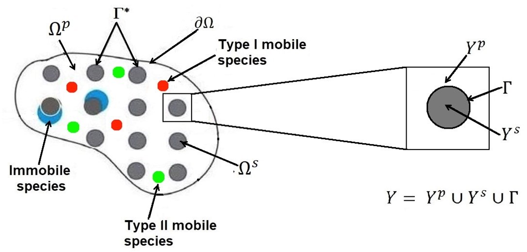
Let Ξ©βŠ‚β„n|nβ‰₯2\Omega\subset\mathbb{R}^{n_{|n\geq 2}} be a periodic bounded domain such that Ξ©:=Ξ©pβˆͺΞ©sassignΞ©superscriptΩ𝑝superscriptΩ𝑠\Omega:=\Omega^{p}\cup\Omega^{s} and Ω¯s∩Ωp=Ο•superscript¯Ω𝑠superscriptΩ𝑝italic-Ο•\bar{\Omega}^{s}\cap\Omega^{p}=\phi, where Ξ©psuperscriptΩ𝑝\Omega^{p} and Ξ©ssuperscriptΩ𝑠\Omega^{s} denotes the pore space and the union of the disconnected solid parts, respectively. βˆ‚Ξ©Ξ©\partial\Omega and Ξ“Ξ΅βˆ—superscriptsubscriptΞ“πœ€\Gamma_{\varepsilon}^{*} are the outer boundary of the domain and the union of boundaries of the solid parts. The unit representative cell Y:=(0,1)nβŠ‚β„nassignπ‘Œsuperscript01𝑛superscriptℝ𝑛Y:=(0,1)^{n}\subset\mathbb{R}^{n} is the union of a solid part Yssuperscriptπ‘Œπ‘ Y^{s} with boundary ΓΓ\Gamma and the pore part Ypsuperscriptπ‘Œπ‘Y^{p} such that Y=YsβˆͺYpπ‘Œsuperscriptπ‘Œπ‘ superscriptπ‘Œπ‘Y=Y^{s}\cup Y^{p}, YΒ―sβŠ‚YsuperscriptΒ―π‘Œπ‘ π‘Œ\bar{Y}^{s}\subset Y and YΒ―s∩YΒ―p=Ξ“superscriptΒ―π‘Œπ‘ superscriptΒ―π‘Œπ‘Ξ“\bar{Y}^{s}\cap\bar{Y}^{p}=\Gamma. The shifted set Ykpsubscriptsuperscriptπ‘Œπ‘π‘˜Y^{p}_{k} is defined by Ykp:=Yp+βˆ‘j=1nej​kjassignsubscriptsuperscriptπ‘Œπ‘π‘˜superscriptπ‘Œπ‘superscriptsubscript𝑗1𝑛subscript𝑒𝑗subscriptπ‘˜π‘—Y^{p}_{k}:=Y^{p}+\sum_{j=1}^{n}e_{j}k_{j}, for k=(k1,k2,β‹―,kn)βˆˆβ„€nπ‘˜subscriptπ‘˜1subscriptπ‘˜2β‹―subscriptπ‘˜π‘›superscript℀𝑛k=(k_{1},k_{2},\cdots,k_{n})\in\mathbb{Z}^{n}, where ejsubscript𝑒𝑗e_{j} is the j𝑗jth unit vector. The union of all shifted subsets Ykpsubscriptsuperscriptπ‘Œπ‘π‘˜Y^{p}_{k} multiplied by Ξ΅πœ€\varepsilon (and confined within ΩΩ\Omega) defined the perforated porous medium ΩΡp:=βˆͺkβˆˆβ„€n{Ρ​Ykp:Ρ​YkpβŠ‚Ξ©}assignsuperscriptsubscriptΞ©πœ€π‘subscriptπ‘˜superscript℀𝑛conditional-setπœ€subscriptsuperscriptπ‘Œπ‘π‘˜πœ€subscriptsuperscriptπ‘Œπ‘π‘˜Ξ©\Omega_{\varepsilon}^{p}:=\cup_{k\in\mathbb{Z}^{n}}\left\{\varepsilon Y^{p}_{k}:\varepsilon Y^{p}_{k}\subset\Omega\right\}. Similarly, ΩΡssuperscriptsubscriptΞ©πœ€π‘ \Omega_{\varepsilon}^{s} and Ξ“Ξ΅βˆ—superscriptsubscriptΞ“πœ€\Gamma_{\varepsilon}^{*} denote the union of the shifted subsets Ykssuperscriptsubscriptπ‘Œπ‘˜π‘ Y_{k}^{s} and Ξ“ksubscriptΞ“π‘˜\Gamma_{k}. The boundary of the pore space βˆ‚Ξ©Ξ΅p:=βˆ‚Ξ©βˆͺΞ“Ξ΅βˆ—assignsuperscriptsubscriptΞ©πœ€π‘Ξ©subscriptsuperscriptΞ“πœ€\partial\Omega_{\varepsilon}^{p}:=\partial\Omega\cup\Gamma^{*}_{\varepsilon}.

Refer to caption
Figure 1: Mobile species in Ξ©psuperscriptΩ𝑝\Omega^{p} with crystal dissolution and precipitation on Ξ“βˆ—superscriptΞ“\Gamma^{*}.

We make the following geometric assumptions: (a)π‘Ž(a) solid parts do not touch each other. They are distributed periodically in the porous medium, (b)𝑏(b) solid parts do not touch the boundary of Yπ‘ŒY, (c)𝑐(c) solid parts do not touch the outer boundary βˆ‚Ξ©Ξ©\partial\Omega. For T>0,S:=[0,T)formulae-sequence𝑇0assign𝑆0𝑇T>0,S:=[0,T) denotes the time interval. We define the volume elements in ΩΩ\Omega and Yπ‘ŒY as d​x𝑑π‘₯dx and d​y𝑑𝑦dy and the surface elements on Ξ“Ξ΅βˆ—,Ξ“superscriptsubscriptΞ“πœ€Ξ“\Gamma_{\varepsilon}^{*},\Gamma by d​σx,d​σy𝑑subscript𝜎π‘₯𝑑subscriptπœŽπ‘¦d\sigma_{x},d\sigma_{y}, respectively. The characteristic function of ΩΡpsuperscriptsubscriptΞ©πœ€π‘\Omega_{\varepsilon}^{p} in ΩΩ\Omega is given by

χΡ​(x)subscriptπœ’πœ€π‘₯\displaystyle\chi_{\varepsilon}(x) ={1if ​x∈ΩΡp,0if ​xβˆˆΞ©βˆ–Ξ©Ξ΅p.\displaystyle\;\;=\;\;\left\{\begin{aligned} &1&&\textnormal{if }x\in\Omega_{\varepsilon}^{p},\\ &0&&\textnormal{if }x\in\Omega\setminus\Omega_{\varepsilon}^{p}.\end{aligned}\right.

According to our consideration, two mobile species M1subscript𝑀1M_{1} and M2subscript𝑀2M_{2} are present in ΩΡpsuperscriptsubscriptΞ©πœ€π‘\Omega_{\varepsilon}^{p}. They are reacting reversibly and forming an immobile species M12subscript𝑀12M_{12} which is accumulating on the interface between the pore space and the solid parts. The reaction amongst the mobile and immobile species is given by

M1+M2↔M12Β onΒ Ξ“Ξ΅βˆ—.↔subscript𝑀1subscript𝑀2subscript𝑀12Β onΒ superscriptsubscriptΞ“πœ€M_{1}+M_{2}\leftrightarrow M_{12}\qquad\text{ on }\quad\Gamma_{\varepsilon}^{*}. (2.1)

We choose the forward reaction rate term as the Langmuir Isotherm and the dissolution rate term is taken as Rd​(wΞ΅)∈kdβ€‹Οˆβ€‹(wΞ΅)subscript𝑅𝑑subscriptπ‘€πœ€subscriptπ‘˜π‘‘πœ“subscriptπ‘€πœ€R_{d}(w_{\varepsilon})\in k_{d}\psi(w_{\varepsilon}), cf. [14, 23, 24], where

Οˆβ€‹(c)πœ“π‘\displaystyle\psi(c) ={{0}if ​c<0,[0,1]if ​c=0,{1}if ​c>0.\displaystyle\;\;=\;\;\left\{\begin{aligned} &\{0\}&&\textnormal{if }c<0,\\ &[0,1]&&\textnormal{if }c=0,\\ &\{1\}&&\textnormal{if }c>0.\end{aligned}\right. (2.2)

We consider the same model as is described in [12]. We denote the concentrations of M1,M2subscript𝑀1subscript𝑀2M_{1},M_{2} and M12subscript𝑀12M_{12} by uΞ΅,vΞ΅subscriptπ‘’πœ€subscriptπ‘£πœ€u_{\varepsilon},v_{\varepsilon} and wΞ΅subscriptπ‘€πœ€w_{\varepsilon}, respectively. All these unknowns are dimensionless. Then the mass-balance equations for M1,M2subscript𝑀1subscript𝑀2M_{1},M_{2} and M12subscript𝑀12M_{12} are given by

βˆ‚uΞ΅βˆ‚t+βˆ‡.(βˆ’DΒ―1β€‹βˆ‡uΞ΅)formulae-sequencesubscriptπ‘’πœ€π‘‘βˆ‡subscript¯𝐷1βˆ‡subscriptπ‘’πœ€\displaystyle\frac{\partial u_{\varepsilon}}{\partial{t}}+\nabla.(-{\bar{D}_{1}}\nabla u_{\varepsilon}) =0​ in ​S×ΩΡp,absent0Β in 𝑆superscriptsubscriptΞ©πœ€π‘\displaystyle=0\;\text{ in }S\times\Omega_{\varepsilon}^{p}, (2.3a)
βˆ’DΒ―1β€‹βˆ‡uΞ΅.nβ†’formulae-sequencesubscript¯𝐷1βˆ‡subscriptπ‘’πœ€β†’π‘›\displaystyle-{\bar{D}_{1}}\nabla u_{\varepsilon}.\vec{n} =0​ on ​SΓ—βˆ‚Ξ©,absent0Β on 𝑆Ω\displaystyle=0\;\text{ on }S\times\partial\Omega, (2.3b)
βˆ’DΒ―1β€‹βˆ‡uΞ΅.nβ†’formulae-sequencesubscript¯𝐷1βˆ‡subscriptπ‘’πœ€β†’π‘›\displaystyle-{\bar{D}_{1}}\nabla u_{\varepsilon}.\vec{n} =Ξ΅β€‹βˆ‚wΞ΅βˆ‚t​ on ​SΓ—Ξ“Ξ΅βˆ—,absentπœ€subscriptπ‘€πœ€π‘‘Β on 𝑆superscriptsubscriptΞ“πœ€\displaystyle=\varepsilon{\frac{\partial w_{\varepsilon}}{\partial{t}}}\;\text{ on }S\times\Gamma_{\varepsilon}^{*}, (2.3c)
uΡ​(0,x)subscriptπ‘’πœ€0π‘₯\displaystyle u_{\varepsilon}(0,x) =uI​Ρ​(x)​ in ​ΩΡp,absentsubscriptπ‘’πΌπœ€π‘₯Β inΒ superscriptsubscriptΞ©πœ€π‘\displaystyle=u_{I\varepsilon}(x)\;\text{ in }\Omega_{\varepsilon}^{p}, (2.3d)
βˆ‚vΞ΅βˆ‚t+βˆ‡.(βˆ’DΒ―2β€‹βˆ‡vΞ΅)formulae-sequencesubscriptπ‘£πœ€π‘‘βˆ‡subscript¯𝐷2βˆ‡subscriptπ‘£πœ€\displaystyle\frac{\partial v_{\varepsilon}}{\partial{t}}+\nabla.(-{\bar{D}_{2}}\nabla v_{\varepsilon}) =0​ in ​S×ΩΡp,absent0Β in 𝑆superscriptsubscriptΞ©πœ€π‘\displaystyle=0\;\text{ in }S\times\Omega_{\varepsilon}^{p}, (2.3e)
βˆ’DΒ―2β€‹βˆ‡vΞ΅.nβ†’formulae-sequencesubscript¯𝐷2βˆ‡subscriptπ‘£πœ€β†’π‘›\displaystyle-{\bar{D}_{2}}\nabla v_{\varepsilon}.\vec{n} =0​ on ​SΓ—βˆ‚Ξ©,absent0Β on 𝑆Ω\displaystyle=0\;\text{ on }S\times\partial\Omega, (2.3f)
βˆ’DΒ―2β€‹βˆ‡vΞ΅.nβ†’formulae-sequencesubscript¯𝐷2βˆ‡subscriptπ‘£πœ€β†’π‘›\displaystyle-{\bar{D}_{2}}\nabla v_{\varepsilon}.\vec{n} =Ξ΅β€‹βˆ‚wΞ΅βˆ‚t​ on ​SΓ—Ξ“Ξ΅βˆ—,absentπœ€subscriptπ‘€πœ€π‘‘Β on 𝑆superscriptsubscriptΞ“πœ€\displaystyle=\varepsilon{\frac{\partial w_{\varepsilon}}{\partial{t}}}\;\text{ on }S\times\Gamma_{\varepsilon}^{*}, (2.3g)
vΡ​(0,x)subscriptπ‘£πœ€0π‘₯\displaystyle v_{\varepsilon}(0,x) =vI​Ρ​(x)​ in ​ΩΡp,absentsubscriptπ‘£πΌπœ€π‘₯Β inΒ superscriptsubscriptΞ©πœ€π‘\displaystyle=v_{I\varepsilon}(x)\;\text{ in }\Omega_{\varepsilon}^{p}, (2.3h)
βˆ‚wΞ΅βˆ‚tsubscriptπ‘€πœ€π‘‘\displaystyle\frac{\partial w_{\varepsilon}}{\partial{t}} =kd​(R​(uΞ΅,vΞ΅)βˆ’zΞ΅)​ on ​SΓ—Ξ“Ξ΅βˆ—,absentsubscriptπ‘˜π‘‘π‘…subscriptπ‘’πœ€subscriptπ‘£πœ€subscriptπ‘§πœ€Β on 𝑆superscriptsubscriptΞ“πœ€\displaystyle=k_{d}(R(u_{\varepsilon},v_{\varepsilon})-z_{\varepsilon})\;\text{ on }S\times\Gamma_{\varepsilon}^{*}, (2.3i)
zΞ΅subscriptπ‘§πœ€\displaystyle z_{\varepsilon} βˆˆΟˆβ€‹(wΞ΅)​ on ​SΓ—Ξ“Ξ΅βˆ—,absentπœ“subscriptπ‘€πœ€Β on 𝑆superscriptsubscriptΞ“πœ€\displaystyle\in\psi(w_{\varepsilon})\;\text{ on }S\times\Gamma_{\varepsilon}^{*}, (2.3j)
wΡ​(0,x)subscriptπ‘€πœ€0π‘₯\displaystyle w_{\varepsilon}(0,x) =wI​Ρ​(x)​ onΒ β€‹Ξ“Ξ΅βˆ—,absentsubscriptπ‘€πΌπœ€π‘₯Β onΒ superscriptsubscriptΞ“πœ€\displaystyle=w_{I\varepsilon}(x)\;\text{ on }\Gamma_{\varepsilon}^{*}, (2.3k)

where R:ℝ2β†’[0,∞):𝑅→superscriptℝ20R:\mathbb{R}^{2}\rightarrow[0,\infty) is defined by

R​(uΞ΅,vΞ΅)𝑅subscriptπ‘’πœ€subscriptπ‘£πœ€\displaystyle R(u_{\varepsilon},v_{\varepsilon}) ={k​k1​uΡ​k2​vΞ΅(1+k1​uΞ΅+k2​vΞ΅)2Β for ​uΞ΅>0,vΞ΅>0,0Β otherwiseΒ \displaystyle\;\;=\;\;\left\{\begin{aligned} &k\frac{k_{1}u_{\varepsilon}k_{2}v_{\varepsilon}}{(1+k_{1}u_{\varepsilon}+k_{2}v_{\varepsilon})^{2}}&&\textnormal{ for }u_{\varepsilon}>0,v_{\varepsilon}>0,\\ &0&&\textnormal{ otherwise }\end{aligned}\right. (2.4)

and k=kfkdπ‘˜subscriptπ‘˜π‘“subscriptπ‘˜π‘‘k=\frac{k_{f}}{k_{d}}. k1subscriptπ‘˜1k_{1} and k2subscriptπ‘˜2k_{2} are the Langmuir parameters for the mobile species M1subscript𝑀1M_{1} and M2subscript𝑀2M_{2}. The rate of dissolution is given by Rd=kdβ€‹Οˆβ€‹(wΞ΅).subscript𝑅𝑑subscriptπ‘˜π‘‘πœ“subscriptπ‘€πœ€R_{d}=k_{d}\psi(w_{\varepsilon}). Also, kfsubscriptπ‘˜π‘“k_{f} is the forward reaction rate constant for precipitation and kdsubscriptπ‘˜π‘‘k_{d} denotes the dissolution rate constant. We denote this problem/model (2.3a)βˆ’(2.3k)2.3a2.3k(\ref{eqn:M11})-(\ref{eqn:MN3}) by (𝒫Ρsubscriptπ’«πœ€\mathcal{P}_{\varepsilon}).

3 Corrector estimate

Let θ∈[0,1]πœƒ01\theta\in[0,1] and r,sβˆˆβ„π‘Ÿπ‘ β„r,s\in\mathbb{R} be such that 1r+1s=11π‘Ÿ1𝑠1\frac{1}{r}+\frac{1}{s}=1. Suppose that Ξ∈{Ξ©,ΩΡp}ΞΩsubscriptsuperscriptΞ©π‘πœ€\Xi\in\{\Omega,\Omega^{p}_{\varepsilon}\}, then Lr​(Ξ)superscriptπΏπ‘ŸΞžL^{r}(\Xi), H1,r​(Ξ)superscript𝐻1π‘ŸΞžH^{1,r}(\Xi), Cθ​(Ξ¯)superscriptπΆπœƒΒ―ΞžC^{\theta}(\overline{\Xi}), (β‹…,β‹…)ΞΈ,rsubscriptβ‹…β‹…πœƒπ‘Ÿ(\cdot,\cdot)_{\theta,r} and [β‹…,β‹…]ΞΈsubscriptβ‹…β‹…πœƒ[\cdot,\cdot]_{\theta} are the Lebesgue, Sobolev, HΓΆlder, real- and complex-interpolation spaces respectively endowed with their standard norms. We define β€–fβ€–Ξžr=∫Ξ|f|r​𝑑xsubscriptsuperscriptnormπ‘“π‘ŸΞžsubscriptΞsuperscriptπ‘“π‘Ÿdifferential-dπ‘₯\|f\|^{r}_{\Xi}=\int_{\Xi}|f|^{r}\,dx and β€–fβ€–(Ξ)tr=∫SΓ—Ξž|f|r​𝑑x​𝑑tsubscriptsuperscriptnormπ‘“π‘ŸsuperscriptΞžπ‘‘subscriptπ‘†Ξžsuperscriptπ‘“π‘Ÿdifferential-dπ‘₯differential-d𝑑\|f\|^{r}_{(\Xi)^{t}}=\int_{S\times\Xi}|f|^{r}\,dx\,dt. The symbols β†ͺβ†ͺ\hookrightarrow, β†ͺβ†ͺβ†ͺabsentβ†ͺ\hookrightarrow\hookrightarrow and dβ†ͺβ†ͺ𝑑\underset{\hookrightarrow}{d} denote the continuous, compact and dense embeddings, respectively. We denote Lr​(Ξ)β†ͺH1,s​(Ξ)βˆ—β†ͺsuperscriptπΏπ‘ŸΞžsuperscript𝐻1𝑠superscriptΞL^{r}(\Xi)\hookrightarrow H^{1,s}(\Xi)^{*} as

⟨f,v⟩H1,s​(Ξ)βˆ—Γ—H1,s​(Ξ)subscript𝑓𝑣superscript𝐻1𝑠superscriptΞsuperscript𝐻1π‘ Ξž\displaystyle\langle f,v\rangle_{H^{1,s}(\Xi)^{*}\times H^{1,s}(\Xi)} =\displaystyle= ⟨f,v⟩Lr​(Ξ)Γ—Ls​(Ξ):=∫Ξf​v​𝑑x​ for ​f∈Lr​(Ξ),v∈H1,s​(Ξ).formulae-sequenceassignsubscript𝑓𝑣superscriptπΏπ‘ŸΞžsuperscriptπΏπ‘ ΞžsubscriptΞžπ‘“π‘£differential-dπ‘₯Β for 𝑓superscriptπΏπ‘ŸΞžπ‘£superscript𝐻1π‘ Ξž\displaystyle\langle f,v\rangle_{L^{r}(\Xi)\times L^{s}(\Xi)}:=\int_{\Xi}fv\,dx\textnormal{ for }f\in L^{r}(\Xi),\;v\in H^{1,s}(\Xi).

We also introduce the Lr​(Ξ“Ξ΅βˆ—)βˆ’Ls​(Ξ“Ξ΅βˆ—)superscriptπΏπ‘ŸsuperscriptsubscriptΞ“πœ€superscript𝐿𝑠superscriptsubscriptΞ“πœ€L^{r}(\Gamma_{\varepsilon}^{*})-L^{s}(\Gamma_{\varepsilon}^{*}) duality as

⟨΢1,ΞΆ2⟩:=Ξ΅β€‹βˆ«Ξ“Ξ΅βˆ—ΞΆ1​΢2​𝑑σx​ for ​΢1∈Lr​(Ξ“Ξ΅βˆ—),ΞΆ2∈Ls​(Ξ“Ξ΅βˆ—)formulae-sequenceassignsubscript𝜁1subscript𝜁2πœ€subscriptsuperscriptsubscriptΞ“πœ€subscript𝜁1subscript𝜁2differential-dsubscript𝜎π‘₯Β forΒ subscript𝜁1superscriptπΏπ‘ŸsuperscriptsubscriptΞ“πœ€subscript𝜁2superscript𝐿𝑠superscriptsubscriptΞ“πœ€\displaystyle\langle\zeta_{1},\zeta_{2}\rangle:=\varepsilon\int_{\Gamma_{\varepsilon}^{*}}\zeta_{1}\zeta_{2}\,d\sigma_{x}\text{ for }\zeta_{1}\in L^{r}(\Gamma_{\varepsilon}^{*}),\;\zeta_{2}\in L^{s}(\Gamma_{\varepsilon}^{*})

and the space Lr​(SΓ—Ξ“Ξ΅βˆ—)superscriptπΏπ‘Ÿπ‘†superscriptsubscriptΞ“πœ€L^{r}(S\times\Gamma_{\varepsilon}^{*}) is equipped with the norm

β€–ΞΆβ€–(Ξ“Ξ΅βˆ—)trsubscriptsuperscriptnormπœπ‘ŸsuperscriptsuperscriptsubscriptΞ“πœ€π‘‘\displaystyle\|\zeta\|^{r}_{(\Gamma_{\varepsilon}^{*})^{t}} :={Ξ΅β€‹βˆ«SΓ—Ξ“Ξ΅βˆ—|΢​(t,x)|r​𝑑σx​𝑑tfor ​1≀r<∞,ess sup(t,x)∈SΓ—Ξ“Ξ΅βˆ—β€‹|΢​(t,x)|for ​r=∞.\displaystyle\;\;:=\;\;\left\{\begin{aligned} &\varepsilon\int_{S\times\Gamma_{\varepsilon}^{*}}|\zeta(t,x)|^{r}\,d\sigma_{x}\,dt&&\textnormal{for }1\leq r<\infty,\\ &\underset{(t,x)\in S\times\Gamma_{\varepsilon}^{*}}{\text{ess sup}}{|\zeta(t,x)|}&&\textnormal{for }r=\infty.\end{aligned}\right.

For more details about the choice of the function spaces and the definition of the function spaces and embedding theorems for the problem (𝒫Ρ)subscriptπ’«πœ€(\mathcal{P}_{\varepsilon}) look into the work [12]. We impose the following assumptions for the sake of analysis:
π€πŸ.π€πŸ\bf A1. uI​Ρ​(x),vI​Ρ​(x),wI​Ρ​(x)β‰₯0.subscriptπ‘’πΌπœ€π‘₯subscriptπ‘£πΌπœ€π‘₯subscriptπ‘€πΌπœ€π‘₯0u_{I\varepsilon}(x),v_{I\varepsilon}(x),w_{I\varepsilon}(x)\geq 0. β€ƒπ€πŸ.π€πŸ\bf A2. R​(uΞ΅,vΞ΅)=0𝑅subscriptπ‘’πœ€subscriptπ‘£πœ€0R(u_{\varepsilon},v_{\varepsilon})=0 for all uΡ≀0,vΡ≀0.formulae-sequencesubscriptπ‘’πœ€0subscriptπ‘£πœ€0u_{\varepsilon}\leq 0,v_{\varepsilon}\leq 0. π€πŸ‘.π€πŸ‘\bf A3. R:ℝ2β†’[0,∞):𝑅→superscriptℝ20R:\mathbb{R}^{2}\rightarrow[0,\infty) is Locally Lipschitz in ℝ2,superscriptℝ2\mathbb{R}^{2}, as

|R​(uΞ΅(1),vΞ΅)βˆ’R​(uΞ΅(2),vΞ΅)|≀LR​|uΞ΅(1)βˆ’uΞ΅(2)|,𝑅superscriptsubscriptπ‘’πœ€1subscriptπ‘£πœ€π‘…superscriptsubscriptπ‘’πœ€2subscriptπ‘£πœ€subscript𝐿𝑅superscriptsubscriptπ‘’πœ€1superscriptsubscriptπ‘’πœ€2\displaystyle|R(u_{\varepsilon}^{(1)},v_{\varepsilon})-R(u_{\varepsilon}^{(2)},v_{\varepsilon})|\leq L_{R}|u_{\varepsilon}^{(1)}-u_{\varepsilon}^{(2)}|,

where LR>0subscript𝐿𝑅0L_{R}>0 is a constant. LR=supLR​(uΞ΅,vΞ΅)subscript𝐿𝑅supremumsubscript𝐿𝑅subscriptπ‘’πœ€subscriptπ‘£πœ€L_{R}=\sup L_{R}(u_{\varepsilon},v_{\varepsilon}) where LR(uΞ΅,vΞ΅)=kk1k2|vΞ΅|(1+k2vΞ΅)2+k12uΞ΅(1)uΞ΅(2)|L_{R}(u_{\varepsilon},v_{\varepsilon})=kk_{1}k_{2}|v_{\varepsilon}|(1+k_{2}v_{\varepsilon})^{2}+k_{1}^{2}u_{\varepsilon}^{(1)}u_{\varepsilon}^{(2)}|. π€πŸ’.π€πŸ’\bf A4. uI​Ρ,vIβ€‹Ξ΅βˆˆL2​(ΩΡp)subscriptπ‘’πΌπœ€subscriptπ‘£πΌπœ€superscript𝐿2subscriptsuperscriptΞ©π‘πœ€u_{I\varepsilon},v_{I\varepsilon}\in L^{2}(\Omega^{p}_{\varepsilon}) and wIβ€‹Ξ΅βˆˆLβˆžβ€‹(Ξ“Ξ΅βˆ—)subscriptπ‘€πΌπœ€superscript𝐿superscriptsubscriptΞ“πœ€w_{I\varepsilon}\in L^{\infty}(\Gamma_{\varepsilon}^{*}). π€πŸ“.π€πŸ“\bf A5. DΒ―1=d​i​a​g​(D1,D1,…,D1)subscript¯𝐷1π‘‘π‘–π‘Žπ‘”subscript𝐷1subscript𝐷1…subscript𝐷1\bar{D}_{1}=diag(D_{1},D_{1},...,D_{1}) and DΒ―2=d​i​a​g​(D2,D2,…,D2)subscript¯𝐷2π‘‘π‘–π‘Žπ‘”subscript𝐷2subscript𝐷2…subscript𝐷2\bar{D}_{2}=diag(D_{2},D_{2},...,D_{2}), where D1,D2subscript𝐷1subscript𝐷2D_{1},D_{2} are positive constants.

3.1 Existence and Homogenization

Theorem 3.1.

Suppose the assumptions (π€πŸ.)βˆ’(π€πŸ“.)(\bf A1.)-(\bf A5.) hold true, then there exists a unique positive weak solution (uΞ΅,vΞ΅,wΞ΅,zΞ΅)subscriptπ‘’πœ€subscriptπ‘£πœ€subscriptπ‘€πœ€subscriptπ‘§πœ€(u_{\varepsilon},v_{\varepsilon},w_{\varepsilon},z_{\varepsilon}) of (𝒫Ρ)subscriptπ’«πœ€(\mathcal{P}_{\varepsilon}) which satisfies

0≀‖uΡ​(t)‖ΩΡp≀Mu,0≀‖vΡ​(t)‖ΩΡp≀Mv​ a.e. in ​S×ΩΡp,formulae-sequence0subscriptnormsubscriptπ‘’πœ€π‘‘superscriptsubscriptΞ©πœ€π‘subscript𝑀𝑒0subscriptnormsubscriptπ‘£πœ€π‘‘superscriptsubscriptΞ©πœ€π‘subscript𝑀𝑣 a.e. in 𝑆superscriptsubscriptΞ©πœ€π‘\displaystyle 0\leq\|u_{\varepsilon}(t)\|_{\Omega_{\varepsilon}^{p}}\leq M_{u},0\leq\|v_{\varepsilon}(t)\|_{\Omega_{\varepsilon}^{p}}\leq M_{v}\text{ a.e. in }S\times{\Omega_{\varepsilon}^{p}}, (3.1a)
0≀‖wΡ​(t)β€–Ξ“Ξ΅βˆ—β‰€Mw,0≀zΡ≀1​ a.e. on ​SΓ—Ξ“Ξ΅βˆ—β€‹Β andformulae-sequence0subscriptnormsubscriptπ‘€πœ€π‘‘superscriptsubscriptΞ“πœ€subscript𝑀𝑀0subscriptπ‘§πœ€1Β a.e. on 𝑆superscriptsubscriptΞ“πœ€Β and\displaystyle 0\leq\|w_{\varepsilon}(t)\|_{\Gamma_{\varepsilon}^{*}}\leq M_{w},0\leq z_{\varepsilon}\leq 1\text{ a.e. on }S\times{\Gamma_{\varepsilon}^{*}}\text{ and } (3.1b)
βˆ₯uΡ​(t)βˆ₯ΩΡp+D1​βˆ₯βˆ‡uΞ΅βˆ₯(ΩΡp)t+βˆ₯βˆ‚tuΞ΅βˆ₯L2​(S;H1,2​(ΩΡp)βˆ—)+βˆ₯vΡ​(t)βˆ₯ΩΡp+D2​βˆ₯βˆ‡vΞ΅βˆ₯(ΩΡp)t+subscriptdelimited-βˆ₯βˆ₯subscriptπ‘’πœ€π‘‘superscriptsubscriptΞ©πœ€π‘subscript𝐷1subscriptdelimited-βˆ₯βˆ₯βˆ‡subscriptπ‘’πœ€superscriptsuperscriptsubscriptΞ©πœ€π‘π‘‘subscriptdelimited-βˆ₯βˆ₯subscript𝑑subscriptπ‘’πœ€superscript𝐿2𝑆superscript𝐻12superscriptsuperscriptsubscriptΞ©πœ€π‘subscriptdelimited-βˆ₯βˆ₯subscriptπ‘£πœ€π‘‘superscriptsubscriptΞ©πœ€π‘limit-fromsubscript𝐷2subscriptdelimited-βˆ₯βˆ₯βˆ‡subscriptπ‘£πœ€superscriptsuperscriptsubscriptΞ©πœ€π‘π‘‘\displaystyle{\left\lVert u_{\varepsilon}(t)\right\rVert}_{\Omega_{\varepsilon}^{p}}+{D_{1}}{\left\lVert\nabla u_{\varepsilon}\right\rVert}_{(\Omega_{\varepsilon}^{p})^{t}}+{\left\lVert\partial_{t}u_{\varepsilon}\right\rVert}_{L^{2}(S;H^{1,2}(\Omega_{\varepsilon}^{p})^{*})}+{\left\lVert v_{\varepsilon}(t)\right\rVert}_{\Omega_{\varepsilon}^{p}}+{D_{2}}{\left\lVert\nabla v_{\varepsilon}\right\rVert}_{(\Omega_{\varepsilon}^{p})^{t}}+
βˆ₯βˆ‚tvΞ΅βˆ₯L2​(S;H1,2​(ΩΡp)βˆ—)+βˆ₯wΡ​(t)βˆ₯Ξ“Ξ΅βˆ—+βˆ₯βˆ‚twΞ΅βˆ₯(Ξ“Ξ΅βˆ—)t≀C,subscriptdelimited-βˆ₯βˆ₯subscript𝑑subscriptπ‘£πœ€superscript𝐿2𝑆superscript𝐻12superscriptsuperscriptsubscriptΞ©πœ€π‘subscriptdelimited-βˆ₯βˆ₯subscriptπ‘€πœ€π‘‘subscriptsuperscriptΞ“πœ€subscriptdelimited-βˆ₯βˆ₯subscript𝑑subscriptπ‘€πœ€superscriptsubscriptsuperscriptΞ“πœ€π‘‘πΆ\displaystyle\qquad\qquad{\left\lVert\partial_{t}v_{\varepsilon}\right\rVert}_{L^{2}(S;H^{1,2}(\Omega_{\varepsilon}^{p})^{*})}+{\left\lVert w_{\varepsilon}(t)\right\rVert}_{\Gamma^{*}_{\varepsilon}}+{\left\lVert\partial_{t}w_{\varepsilon}\right\rVert}_{{(\Gamma^{*}_{\varepsilon})}^{t}}\leq C, (3.1c)

for a.e. t∈S𝑑𝑆t\in S, where C𝐢C is a generic constant independent of Ξ΅πœ€\varepsilon.

Proof.

We employ Banach’s fixed point theorem to establish the existence of the weak solution. The proof is done in [12]. ∎

Theorem 3.2.

Under the assumptions (π€πŸ.)βˆ’(π€πŸ“.)({\bf A1.})-({\bf A5.}), there exist (u0,v0,w0,z0)∈L2​(S;H1,2​(Ξ©))Γ—L2​(S;H1,2​(Ξ©))Γ—L2​(S;L2​(Ω×Γ))Γ—Lβˆžβ€‹(S×Ω×Γ)subscript𝑒0subscript𝑣0subscript𝑀0subscript𝑧0superscript𝐿2𝑆superscript𝐻12Ξ©superscript𝐿2𝑆superscript𝐻12Ξ©superscript𝐿2𝑆superscript𝐿2ΩΓsuperscript𝐿𝑆ΩΓ(u_{0},v_{0},w_{0},z_{0})\in L^{2}(S;H^{1,2}(\Omega))\times L^{2}(S;H^{1,2}(\Omega))\times L^{2}(S;L^{2}(\Omega\times\Gamma))\times L^{\infty}(S\times\Omega\times\Gamma) such that (u0,v0,w0,z0)subscript𝑒0subscript𝑣0subscript𝑀0subscript𝑧0(u_{0},v_{0},w_{0},z_{0}) is the unique solution of the problem

βˆ‚u0βˆ‚tβˆ’βˆ‡.(Aβ€‹βˆ‡u0)+P​(t,x)formulae-sequencesubscript𝑒0π‘‘βˆ‡π΄βˆ‡subscript𝑒0𝑃𝑑π‘₯\displaystyle\frac{\partial u_{0}}{\partial t}-\nabla.(A\nabla u_{0})+P(t,x) =0inSΓ—Ξ©,absent0in𝑆Ω\displaystyle=0\quad\text{in}\quad S\times\Omega, (3.2a)
βˆ’Aβ€‹βˆ‡u0.nβ†’formulae-sequenceπ΄βˆ‡subscript𝑒0→𝑛\displaystyle-A\nabla u_{0}.\vec{n} =0onSΓ—βˆ‚Ξ©,absent0on𝑆Ω\displaystyle=0\quad\text{on}\quad S\times\partial\Omega, (3.2b)
u0​(0,x)=subscript𝑒00π‘₯absent\displaystyle u_{0}(0,x)= uI​0​(x)inΞ©,subscript𝑒𝐼0π‘₯inΞ©\displaystyle u_{I0}(x)\quad\text{in}\quad\Omega, (3.2c)
βˆ‚v0βˆ‚tβˆ’βˆ‡.(Bβ€‹βˆ‡v0)+P​(t,x)formulae-sequencesubscript𝑣0π‘‘βˆ‡π΅βˆ‡subscript𝑣0𝑃𝑑π‘₯\displaystyle\frac{\partial v_{0}}{\partial t}-\nabla.(B\nabla v_{0})+P(t,x) =0inSΓ—Ξ©,absent0in𝑆Ω\displaystyle=0\quad\text{in}\quad S\times\Omega, (3.3a)
βˆ’Bβ€‹βˆ‡v0.nβ†’formulae-sequenceπ΅βˆ‡subscript𝑣0→𝑛\displaystyle-B\nabla v_{0}.\vec{n} =0onSΓ—βˆ‚Ξ©,absent0on𝑆Ω\displaystyle=0\quad\text{on}\quad S\times\partial\Omega, (3.3b)
v0​(0,x)subscript𝑣00π‘₯\displaystyle v_{0}(0,x) =vI​0​(x)inΞ©,absentsubscript𝑣𝐼0π‘₯inΞ©\displaystyle=v_{I0}(x)\quad\text{in}\quad\Omega, (3.3c)
βˆ‚w0βˆ‚t=kd​(R​(u0,v0)βˆ’z0)inS×Ω×Γ,subscript𝑀0𝑑subscriptπ‘˜π‘‘π‘…subscript𝑒0subscript𝑣0subscript𝑧0in𝑆ΩΓ\displaystyle\frac{\partial w_{0}}{\partial t}=k_{d}(R(u_{0},v_{0})-z_{0})\quad\text{in}\quad S\times\Omega\times\Gamma, (3.4a)
Β where ​z0βˆˆΟˆβ€‹(w0)inS×Ω×Γ,Β whereΒ subscript𝑧0πœ“subscript𝑀0in𝑆ΩΓ\displaystyle\;\text{ where }z_{0}\in\psi(w_{0})\quad\text{in}\quad S\times\Omega\times\Gamma, (3.4b)
w0​(0,x,y)=wI​0​(x,y)onΩ×Γ,subscript𝑀00π‘₯𝑦subscript𝑀𝐼0π‘₯𝑦onΩΓ\displaystyle w_{0}(0,x,y)=w_{I0}(x,y)\quad\text{on}\quad\Omega\times\Gamma, (3.4c)

satisfying the a-priori bound

β€–u0β€–(Ξ©)tsubscriptnormsubscript𝑒0superscriptΩ𝑑\displaystyle\|u_{0}\|_{(\Omega)^{t}} +β€–βˆ‡u0β€–(Ξ©)t+β€–βˆ‚tu0β€–L2​(S;H1,2​(Ξ©)βˆ—)+β€–v0β€–(Ξ©)t+β€–βˆ‡v0β€–(Ξ©)t+β€–βˆ‚tv0β€–L2​(S;H1,2​(Ξ©)βˆ—)subscriptnormβˆ‡subscript𝑒0superscriptΩ𝑑subscriptnormsubscript𝑑subscript𝑒0superscript𝐿2𝑆superscript𝐻12superscriptΞ©subscriptnormsubscript𝑣0superscriptΩ𝑑subscriptnormβˆ‡subscript𝑣0superscriptΩ𝑑subscriptnormsubscript𝑑subscript𝑣0superscript𝐿2𝑆superscript𝐻12superscriptΞ©\displaystyle+\|\nabla u_{0}\|_{(\Omega)^{t}}+\|\partial_{t}u_{0}\|_{L^{2}(S;H^{1,2}(\Omega)^{*})}+\|v_{0}\|_{(\Omega)^{t}}+\|\nabla v_{0}\|_{(\Omega)^{t}}+\|\partial_{t}v_{0}\|_{L^{2}(S;H^{1,2}(\Omega)^{*})}
+β€–w0β€–(Ω×Γ)t+β€–βˆ‚tw0β€–(Ω×Γ)t+β€–Pβ€–(Ξ©)t≀C<∞,subscriptnormsubscript𝑀0superscriptΩΓ𝑑subscriptnormsubscript𝑑subscript𝑀0superscriptΩΓ𝑑subscriptnorm𝑃superscriptΩ𝑑𝐢\displaystyle+\|w_{0}\|_{(\Omega\times\Gamma)^{t}}+\|\partial_{t}w_{0}\|_{(\Omega\times\Gamma)^{t}}+\|P\|_{(\Omega)^{t}}\leq C<\infty, (3.5)

where

P​(t,x)=βˆ«Ξ“1|Yp|β€‹βˆ‚w0βˆ‚t​𝑑σy𝑃𝑑π‘₯subscriptΞ“1superscriptπ‘Œπ‘subscript𝑀0𝑑differential-dsubscriptπœŽπ‘¦\displaystyle P(t,x)=\int_{\Gamma}\frac{1}{|Y^{p}|}\frac{\partial w_{0}}{\partial t}\;d\sigma_{y}

and the elliptic homogenized matrix A=(ai​j)1≀i,j≀n𝐴subscriptsubscriptπ‘Žπ‘–π‘—formulae-sequence1𝑖𝑗𝑛A=(a_{ij})_{1\leq i,j\leq n} and B=(bi​j)1≀i,j≀n𝐡subscriptsubscript𝑏𝑖𝑗formulae-sequence1𝑖𝑗𝑛B=(b_{ij})_{1\leq i,j\leq n} are defined by

ai​j=∫YpD1|Yp|​(Ξ΄i​j+βˆ‘i,j=1nβˆ‚ljβˆ‚yi)​𝑑y,bi​j=∫YpD2|Yp|​(Ξ΄i​j+βˆ‘i,j=1nβˆ‚ljβˆ‚yi)​𝑑y.formulae-sequencesubscriptπ‘Žπ‘–π‘—subscriptsuperscriptπ‘Œπ‘subscript𝐷1superscriptπ‘Œπ‘subscript𝛿𝑖𝑗superscriptsubscript𝑖𝑗1𝑛subscript𝑙𝑗subscript𝑦𝑖differential-d𝑦subscript𝑏𝑖𝑗subscriptsuperscriptπ‘Œπ‘subscript𝐷2superscriptπ‘Œπ‘subscript𝛿𝑖𝑗superscriptsubscript𝑖𝑗1𝑛subscript𝑙𝑗subscript𝑦𝑖differential-d𝑦\displaystyle a_{ij}=\int_{Y^{p}}\frac{D_{1}}{|Y^{p}|}\left(\delta_{ij}+\sum_{i,j=1}^{n}\frac{\partial l_{j}}{\partial y_{i}}\right)dy,\quad b_{ij}=\int_{Y^{p}}\frac{D_{2}}{|Y^{p}|}\left(\delta_{ij}+\sum_{i,j=1}^{n}\frac{\partial l_{j}}{\partial y_{i}}\right)dy.

Moreover, lj∈Hp​e​r1,2​(Yp)subscript𝑙𝑗subscriptsuperscript𝐻12π‘π‘’π‘Ÿsuperscriptπ‘Œπ‘l_{j}\in H^{1,2}_{per}(Y^{p}) are the solutions of the cell problems

{βˆ‡y.(βˆ‡ylj+ej)=0for ally∈Yp,(βˆ‡ylj+ej).nβ†’=0onΞ“,y↦lj​(y)​ is ​Yβˆ’periodic,casesformulae-sequencesubscriptβˆ‡π‘¦formulae-sequencesubscriptβˆ‡π‘¦subscript𝑙𝑗subscript𝑒𝑗0for all𝑦superscriptπ‘Œπ‘otherwiseformulae-sequencesubscriptβˆ‡π‘¦subscript𝑙𝑗subscript𝑒𝑗→𝑛0onΞ“otherwisemaps-to𝑦subscript𝑙𝑗𝑦 isΒ π‘Œperiodicotherwise\displaystyle\begin{cases}\nabla_{y}.(\nabla_{y}l_{j}+e_{j})=0\quad\text{for all}\quad y\in Y^{p},\\ (\nabla_{y}l_{j}+e_{j}).\vec{n}=0\quad\text{on}\quad\Gamma,\\ y\mapsto l_{j}(y)\text{ is }Y-\text{periodic},\end{cases} (3.6)

for j=1,2,β‹―,n𝑗12⋯𝑛j=1,2,\cdots,n and for almost every x∈Ωπ‘₯Ξ©x\in\Omega.

Proof.

We prove the theorem by using homogenization techniques such as two-scale convergence and boundary unfolding operator in [12]. ∎

The main result of this paper is stated in the next Theorem.

Theorem 3.3.

Suppose that

(a)​uIβ€‹Ξ΅βˆˆH1,2​(ΩΡp),π‘Žsubscriptπ‘’πΌπœ€superscript𝐻12superscriptsubscriptΞ©πœ€π‘\displaystyle(a)u_{I\varepsilon}\in H^{1,2}(\Omega_{\varepsilon}^{p}), (3.7)
(b)​limΞ΅β†’0Ξ΅β€‹βˆ«Ξ“Ξ΅βˆ—wI​Ρ2​𝑑σx=βˆ«Ξ©βˆ«Ξ“wI​02​𝑑x​𝑑σy.𝑏subscriptβ†’πœ€0πœ€subscriptsuperscriptsubscriptΞ“πœ€subscriptsuperscript𝑀2πΌπœ€differential-dsubscript𝜎π‘₯subscriptΞ©subscriptΞ“subscriptsuperscript𝑀2𝐼0differential-dπ‘₯differential-dsubscriptπœŽπ‘¦\displaystyle(b)\lim_{\varepsilon\rightarrow 0}\varepsilon\int_{\Gamma_{\varepsilon}^{*}}w^{2}_{I\varepsilon}d\sigma_{x}=\int_{\Omega}\int_{\Gamma}w^{2}_{I0}dxd\sigma_{y}. (3.8)

Now let uΞ΅,vΞ΅,wΞ΅subscriptπ‘’πœ€subscriptπ‘£πœ€subscriptπ‘€πœ€u_{\varepsilon},v_{\varepsilon},w_{\varepsilon} be the solution of the micro problem (​2.3a​)βˆ’(​2.3k​)italic-(2.3aitalic-)italic-(2.3kitalic-)\eqref{eqn:M11}-\eqref{eqn:MN3} and u0,v0,w0subscript𝑒0subscript𝑣0subscript𝑀0u_{0},v_{0},w_{0} are the solutions of the macro problem (​3.2a​)βˆ’(​3.4c​)italic-(3.2aitalic-)italic-(3.4citalic-)\eqref{eqn:M1s1}-\eqref{eqn:M3S3} then the following convergence holds

{(i)​‖uΞ΅βˆ’u0β€–C​([0,T];L2​(ΩΡp))β†’0,(i​i)β€‹β€–βˆ‡uΞ΅βˆ’CΞ΅β€‹βˆ‡u0β€–L2​(0,T;L2​(ΩΡp))β†’0,(i​i​i)​‖vΞ΅βˆ’v0β€–C​([0,T];L2​(ΩΡp))β†’0,(i​v)β€‹β€–βˆ‡vΞ΅βˆ’CΞ΅β€‹βˆ‡v0β€–L2​(0,T;L2​(ΩΡp))β†’0.(v)​‖wΞ΅βˆ’w0β€–C​([0,T];L2​(Ξ“Ξ΅βˆ—))β†’0.casesformulae-sequence→𝑖subscriptnormsubscriptπ‘’πœ€subscript𝑒0𝐢0𝑇superscript𝐿2superscriptsubscriptΞ©πœ€π‘0→𝑖𝑖subscriptnormβˆ‡subscriptπ‘’πœ€superscriptπΆπœ€βˆ‡subscript𝑒0superscript𝐿20𝑇superscript𝐿2superscriptsubscriptΞ©πœ€π‘0otherwiseformulae-sequence→𝑖𝑖𝑖subscriptnormsubscriptπ‘£πœ€subscript𝑣0𝐢0𝑇superscript𝐿2superscriptsubscriptΞ©πœ€π‘0→𝑖𝑣subscriptnormβˆ‡subscriptπ‘£πœ€superscriptπΆπœ€βˆ‡subscript𝑣0superscript𝐿20𝑇superscript𝐿2superscriptsubscriptΞ©πœ€π‘0otherwise→𝑣subscriptnormsubscriptπ‘€πœ€subscript𝑀0𝐢0𝑇superscript𝐿2superscriptsubscriptΞ“πœ€0otherwise\displaystyle\begin{cases}(i)\|u_{\varepsilon}-u_{0}\|_{C([0,T];L^{2}(\Omega_{\varepsilon}^{p}))}\rightarrow 0,\quad(ii)\|\nabla u_{\varepsilon}-C^{\varepsilon}\nabla u_{0}\|_{L^{2}(0,T;L^{2}(\Omega_{\varepsilon}^{p}))}\rightarrow 0,\\ (iii)\|v_{\varepsilon}-v_{0}\|_{C([0,T];L^{2}(\Omega_{\varepsilon}^{p}))}\rightarrow 0,\quad(iv)\|\nabla v_{\varepsilon}-C^{\varepsilon}\nabla v_{0}\|_{L^{2}(0,T;L^{2}(\Omega_{\varepsilon}^{p}))}\rightarrow 0.\\ (v)\|w_{\varepsilon}-w_{0}\|_{C([0,T];L^{2}(\Gamma_{\varepsilon}^{*}))}\rightarrow 0.\end{cases} (3.9)

3.2 Convergence of the energy

We define the energies associated with the mobile species M1subscript𝑀1M_{1} of the micromodel and the macromodel as

EΡ​(t)=12β€‹βˆ«Ξ©Ξ΅puΞ΅2​(t)​𝑑x+∫0t∫ΩΡpD1β€‹βˆ‡uΡ​(Ο„,x)β€‹βˆ‡uΡ​(Ο„,x)​𝑑x​𝑑τ,subscriptπΈπœ€π‘‘12subscriptsuperscriptsubscriptΞ©πœ€π‘subscriptsuperscript𝑒2πœ€π‘‘differential-dπ‘₯superscriptsubscript0𝑑subscriptsuperscriptsubscriptΞ©πœ€π‘subscript𝐷1βˆ‡subscriptπ‘’πœ€πœπ‘₯βˆ‡subscriptπ‘’πœ€πœπ‘₯differential-dπ‘₯differential-d𝜏\displaystyle E_{\varepsilon}(t)=\frac{1}{2}\int_{\Omega_{\varepsilon}^{p}}u^{2}_{\varepsilon}(t)dx+\int_{0}^{t}\int_{\Omega_{\varepsilon}^{p}}D_{1}\nabla u_{\varepsilon}(\tau,x)\nabla u_{\varepsilon}(\tau,x)dxd\tau, (3.10)
E0​(t)=|Yp|2β€‹βˆ«Ξ©u02​(t)​𝑑x+|Yp|β€‹βˆ«0t∫ΩAβ€‹βˆ‡u0​(Ο„,x)β€‹βˆ‡u0​(Ο„,x)​𝑑x​𝑑τ.subscript𝐸0𝑑superscriptπ‘Œπ‘2subscriptΞ©subscriptsuperscript𝑒20𝑑differential-dπ‘₯superscriptπ‘Œπ‘superscriptsubscript0𝑑subscriptΞ©π΄βˆ‡subscript𝑒0𝜏π‘₯βˆ‡subscript𝑒0𝜏π‘₯differential-dπ‘₯differential-d𝜏\displaystyle E_{0}(t)=\frac{|Y^{p}|}{2}\int_{\Omega}u^{2}_{0}(t)dx+|Y^{p}|\int_{0}^{t}\int_{\Omega}A\nabla u_{0}(\tau,x)\nabla u_{0}(\tau,x)dxd\tau. (3.11)

We choose uΡ​(t,x),u0​(t,x)subscriptπ‘’πœ€π‘‘π‘₯subscript𝑒0𝑑π‘₯u_{\varepsilon}(t,x),u_{0}(t,x) as the test functions in the equations (2.3a) and (3.2a) and see that the energy terms can be expressed as

EΡ​(t)=12β€‹βˆ«Ξ©Ξ΅puI​Ρ2​𝑑xβˆ’Ξ΅β€‹βˆ«0tβˆ«Ξ“Ξ΅βˆ—βˆ‚wΞ΅βˆ‚t​(Ο„,x)​uΡ​(Ο„,x)​𝑑σx​𝑑τ,subscriptπΈπœ€π‘‘12subscriptsuperscriptsubscriptΞ©πœ€π‘superscriptsubscriptπ‘’πΌπœ€2differential-dπ‘₯πœ€superscriptsubscript0𝑑subscriptsuperscriptsubscriptΞ“πœ€subscriptπ‘€πœ€π‘‘πœπ‘₯subscriptπ‘’πœ€πœπ‘₯differential-dsubscript𝜎π‘₯differential-d𝜏\displaystyle E_{\varepsilon}(t)=\frac{1}{2}\int_{\Omega_{\varepsilon}^{p}}u_{I\varepsilon}^{2}dx-\varepsilon\int_{0}^{t}\int_{\Gamma_{\varepsilon}^{*}}\frac{\partial w_{\varepsilon}}{\partial t}(\tau,x)u_{\varepsilon}(\tau,x)d\sigma_{x}d\tau, (3.12)
E0​(t)=|Yp|2β€‹βˆ«Ξ©uI​02​𝑑xβˆ’βˆ«0tβˆ«Ξ©βˆ«Ξ“βˆ‚w0βˆ‚t​(Ο„,x,y)​u0​(Ο„,x)​𝑑x​𝑑σy​𝑑τ.subscript𝐸0𝑑superscriptπ‘Œπ‘2subscriptΞ©superscriptsubscript𝑒𝐼02differential-dπ‘₯superscriptsubscript0𝑑subscriptΞ©subscriptΞ“subscript𝑀0π‘‘πœπ‘₯𝑦subscript𝑒0𝜏π‘₯differential-dπ‘₯differential-dsubscriptπœŽπ‘¦differential-d𝜏\displaystyle E_{0}(t)=\frac{|Y^{p}|}{2}\int_{\Omega}u_{I0}^{2}dx-\int_{0}^{t}\int_{\Omega}\int_{\Gamma}\frac{\partial w_{0}}{\partial t}(\tau,x,y)u_{0}(\tau,x)dxd\sigma_{y}d\tau. (3.13)

The following convergence holds true for the energies:

Lemma 3.4.

EΡ​(t)β†’E0​(t)β†’subscriptπΈπœ€π‘‘subscript𝐸0𝑑E_{\varepsilon}(t)\rightarrow E_{0}(t) strongly C​([0,T])𝐢0𝑇C([0,T]) under the condition (3.7).

Proof.

We have to show that EΡ​(t)∈C​[0,T]subscriptπΈπœ€π‘‘πΆ0𝑇E_{\varepsilon}(t)\in C[0,T]. As a consequence of Arzela-Ascoli theorem, it is equivalent to establish the followings:
(i)​|EΡ​(t)|≀C𝑖subscriptπΈπœ€π‘‘πΆ(i)|E_{\varepsilon}(t)|\leq C for all t∈[0,T]𝑑0𝑇t\in[0,T].
(i​i)​|EΡ​(t+h)βˆ’EΡ​(t)|≀θ​(h)𝑖𝑖subscriptπΈπœ€π‘‘β„ŽsubscriptπΈπœ€π‘‘πœƒβ„Ž(ii)|E_{\varepsilon}(t+h)-E_{\varepsilon}(t)|\leq\theta(h) uniformly with respect to Ξ΅πœ€\varepsilon for all t∈[0,Tβˆ’h)𝑑0π‘‡β„Žt\in[0,T-h) for all h>0β„Ž0h>0 and θ​(h)β†’0β†’πœƒβ„Ž0\theta(h)\rightarrow 0 as hβ†’0β†’β„Ž0h\rightarrow 0.
We use Theorem 3.1 to estimate EΡ​(t)subscriptπΈπœ€π‘‘E_{\varepsilon}(t) and obtain

|EΡ​(t)|≀12​‖uI​Ρ‖ΩΡp2+kd22​(1+k4)2​T​|Ξ“|​|Ξ©||Y|+C2​[β€–uΞ΅β€–(ΩΡp)t2+β€–βˆ‡uΞ΅β€–(ΩΡp)t2]=C.subscriptπΈπœ€π‘‘12subscriptsuperscriptnormsubscriptπ‘’πΌπœ€2superscriptsubscriptΞ©πœ€π‘superscriptsubscriptπ‘˜π‘‘22superscript1π‘˜42π‘‡Ξ“Ξ©π‘ŒπΆ2delimited-[]subscriptsuperscriptnormsubscriptπ‘’πœ€2superscriptsuperscriptsubscriptΞ©πœ€π‘π‘‘subscriptsuperscriptnormβˆ‡subscriptπ‘’πœ€2superscriptsuperscriptsubscriptΞ©πœ€π‘π‘‘πΆ\displaystyle|E_{\varepsilon}(t)|\leq\frac{1}{2}\|u_{I\varepsilon}\|^{2}_{\Omega_{\varepsilon}^{p}}+\frac{k_{d}^{2}}{2}(1+\frac{k}{4})^{2}\frac{T|\Gamma||\Omega|}{|Y|}+\frac{C}{2}\left[\|u_{\varepsilon}\|^{2}_{(\Omega_{\varepsilon}^{p})^{t}}+\|\nabla u_{\varepsilon}\|^{2}_{(\Omega_{\varepsilon}^{p})^{t}}\right]=C.

Hence (i)𝑖(i) proved. Next, to show (i​i)𝑖𝑖(ii) we consider (3.12) and utilize the a-priori bounds of Theorem 3.1 and deduce

|EΡ​(t+h)βˆ’EΡ​(t)|subscriptπΈπœ€π‘‘β„ŽsubscriptπΈπœ€π‘‘\displaystyle\left|E_{\varepsilon}(t+h)-E_{\varepsilon}(t)\right| =|Ξ΅β€‹βˆ«tt+hβˆ«Ξ“Ξ΅βˆ—βˆ‚wΞ΅βˆ‚t​uΡ​𝑑σx​𝑑τ|absentπœ€superscriptsubscriptπ‘‘π‘‘β„ŽsubscriptsuperscriptsubscriptΞ“πœ€subscriptπ‘€πœ€π‘‘subscriptπ‘’πœ€differential-dsubscript𝜎π‘₯differential-d𝜏\displaystyle=\left|\varepsilon\int_{t}^{t+h}\int_{\Gamma_{\varepsilon}^{*}}\frac{\partial w_{\varepsilon}}{\partial t}u_{\varepsilon}d\sigma_{x}d\tau\right|
≀C​h12​‖uΞ΅β€–Lβˆžβ€‹(S;H1,2​(ΩΡp))​βˆ₯βˆ‚wΞ΅βˆ‚tβˆ₯L2​(SΓ—Ξ“Ξ΅βˆ—)=C1​h12.absent𝐢superscriptβ„Ž12subscriptnormsubscriptπ‘’πœ€superscript𝐿𝑆superscript𝐻12superscriptsubscriptΞ©πœ€π‘subscriptdelimited-βˆ₯βˆ₯subscriptπ‘€πœ€π‘‘superscript𝐿2𝑆superscriptsubscriptΞ“πœ€subscript𝐢1superscriptβ„Ž12\displaystyle\leq Ch^{\frac{1}{2}}\|u_{\varepsilon}\|_{L^{\infty}(S;H^{1,2}(\Omega_{\varepsilon}^{p}))}\left\lVert\frac{\partial w_{\varepsilon}}{\partial t}\right\rVert_{L^{2}(S\times\Gamma_{\varepsilon}^{*})}=C_{1}h^{\frac{1}{2}}.

Therefore upto a subsequence EΡ​(t)β†’ΞΎβ†’subscriptπΈπœ€π‘‘πœ‰E_{\varepsilon}(t)\rightarrow\xi strongly in C​[0,T]𝐢0𝑇C[0,T]. It remains to prove that ΞΎ=E0​(t)πœ‰subscript𝐸0𝑑\xi=E_{0}(t). To do so we pass the limit in EΡ​(t)subscriptπΈπœ€π‘‘E_{\varepsilon}(t) and by Lemma 6.26.26.2 of [12], we get

limΞ΅β†’0EΡ​(t)subscriptβ†’πœ€0subscriptπΈπœ€π‘‘\displaystyle\lim_{\varepsilon\rightarrow 0}E_{\varepsilon}(t) =12​limΞ΅β†’0∫ΩΡpuI​Ρ2​𝑑xβˆ’limΞ΅β†’0Ξ΅β€‹βˆ«0tβˆ«Ξ“Ξ΅βˆ—βˆ‚wΞ΅βˆ‚t​(Ο„,x)​uΡ​(Ο„,x)​𝑑σx​𝑑τabsent12subscriptβ†’πœ€0subscriptsuperscriptsubscriptΞ©πœ€π‘superscriptsubscriptπ‘’πΌπœ€2differential-dπ‘₯subscriptβ†’πœ€0πœ€superscriptsubscript0𝑑subscriptsuperscriptsubscriptΞ“πœ€subscriptπ‘€πœ€π‘‘πœπ‘₯subscriptπ‘’πœ€πœπ‘₯differential-dsubscript𝜎π‘₯differential-d𝜏\displaystyle=\frac{1}{2}\lim_{\varepsilon\rightarrow 0}\int_{\Omega_{\varepsilon}^{p}}u_{I\varepsilon}^{2}dx-\lim_{\varepsilon\rightarrow 0}\varepsilon\int_{0}^{t}\int_{\Gamma_{\varepsilon}^{*}}\frac{\partial w_{\varepsilon}}{\partial t}(\tau,x)u_{\varepsilon}(\tau,x)d\sigma_{x}d\tau
=|Yp|2β€‹βˆ«Ξ©uI​02​𝑑xβˆ’βˆ«0tβˆ«Ξ©βˆ«Ξ“βˆ‚w0βˆ‚t​(Ο„,x,y)​u0​(Ο„,x)​𝑑x​𝑑σy​𝑑τabsentsuperscriptπ‘Œπ‘2subscriptΞ©superscriptsubscript𝑒𝐼02differential-dπ‘₯superscriptsubscript0𝑑subscriptΞ©subscriptΞ“subscript𝑀0π‘‘πœπ‘₯𝑦subscript𝑒0𝜏π‘₯differential-dπ‘₯differential-dsubscriptπœŽπ‘¦differential-d𝜏\displaystyle=\frac{|Y^{p}|}{2}\int_{\Omega}u_{I0}^{2}dx-\int_{0}^{t}\int_{\Omega}\int_{\Gamma}\frac{\partial w_{0}}{\partial t}(\tau,x,y)u_{0}(\tau,x)dxd\sigma_{y}d\tau
=E0​(t).absentsubscript𝐸0𝑑\displaystyle=E_{0}(t).

∎

3.3 Derivation of the corrector estimate

The corrector matrix CΞ΅=(Ci​jΞ΅)1≀i,j≀nsuperscriptπΆπœ€subscriptsubscriptsuperscriptπΆπœ€π‘–π‘—formulae-sequence1𝑖𝑗𝑛C^{\varepsilon}=(C^{\varepsilon}_{ij})_{1\leq i,j\leq n} is defined by

{Ci​jΡ​(x)=ci​j​(xΞ΅)​ a.e. on ​ΩΡp,Ci​j​(y)=Ξ΄i​j+βˆ‚lj​(y)βˆ‚yi=βˆ‚hjΞ΅βˆ‚yi​(y)​ a.e. on ​Yp,casessubscriptsuperscriptπΆπœ€π‘–π‘—π‘₯subscript𝑐𝑖𝑗π‘₯πœ€Β a.e. onΒ superscriptsubscriptΞ©πœ€π‘otherwisesubscript𝐢𝑖𝑗𝑦subscript𝛿𝑖𝑗subscript𝑙𝑗𝑦subscript𝑦𝑖subscriptsuperscriptβ„Žπœ€π‘—subscript𝑦𝑖𝑦 a.e. onΒ superscriptπ‘Œπ‘otherwise\displaystyle\begin{cases}C^{\varepsilon}_{ij}(x)=c_{ij}(\frac{x}{\varepsilon})\text{ a.e. on }\Omega_{\varepsilon}^{p},\\ C_{ij}(y)=\delta_{ij}+\frac{\partial l_{j}(y)}{\partial y_{i}}=\frac{\partial h^{\varepsilon}_{j}}{\partial y_{i}}(y)\text{ a.e. on }Y^{p},\end{cases}

where ljsubscript𝑙𝑗l_{j} is given by (3.6) and hjΞ΅=ej.y+lj​(y)∈Hp​e​r1,2​(Yp)formulae-sequencesubscriptsuperscriptβ„Žπœ€π‘—subscript𝑒𝑗𝑦subscript𝑙𝑗𝑦subscriptsuperscript𝐻12π‘π‘’π‘Ÿsuperscriptπ‘Œπ‘h^{\varepsilon}_{j}=e_{j}.y+l_{j}(y)\in H^{1,2}_{per}(Y^{p}) is Yβˆ’limit-fromπ‘ŒY-periodic and satisfies

{βˆ‡y.(βˆ‡yhjΞ΅)=0for ally∈Yp,βˆ‡yhjΞ΅.nβ†’=0onΞ“,(hjΞ΅βˆ’ej.y)Β isΒ Yβˆ’periodic,\displaystyle\begin{cases}\nabla_{y}.(\nabla_{y}h^{\varepsilon}_{j})=0\quad\text{for all}\quad y\in Y^{p},\\ \nabla_{y}h^{\varepsilon}_{j}.\vec{n}=0\quad\text{on}\quad\Gamma,\\ (h^{\varepsilon}_{j}-e_{j}.y)\text{ is }Y-\text{periodic},\end{cases} (3.14)

for j=1,2,β‹―,n𝑗12⋯𝑛j=1,2,\cdots,n.

Lemma 3.5.

The sequence {hjΞ΅}subscriptsuperscriptβ„Žπœ€π‘—\{h^{\varepsilon}_{j}\} is weakly convergent to hjsubscriptβ„Žπ‘—h_{j} in Hp​e​r1,2​(Yp)subscriptsuperscript𝐻12π‘π‘’π‘Ÿsuperscriptπ‘Œπ‘H^{1,2}_{per}(Y^{p}), where hjsubscriptβ„Žπ‘—h_{j} is the solution of

{βˆ‡y.(βˆ‡yhj)=0for ally∈Yp,βˆ‡yhj.nβ†’=0onΞ“,(hjβˆ’ej.y)Β isΒ Yβˆ’periodic,\displaystyle\begin{cases}\nabla_{y}.(\nabla_{y}h_{j})=0\quad\text{for all}\quad y\in Y^{p},\\ \nabla_{y}h_{j}.\vec{n}=0\quad\text{on}\quad\Gamma,\\ (h_{j}-e_{j}.y)\text{ is }Y-\text{periodic},\end{cases} (3.15)

for j=1,2,β‹―,n𝑗12⋯𝑛j=1,2,\cdots,n.

Proof.

We can see that β€–hjΞ΅β€–Hp​e​r1,2​(Yp)≀Csubscriptnormsubscriptsuperscriptβ„Žπœ€π‘—subscriptsuperscript𝐻12π‘π‘’π‘Ÿsuperscriptπ‘Œπ‘πΆ\|h^{\varepsilon}_{j}\|_{H^{1,2}_{per}(Y^{p})}\leq C, where C𝐢C is a constant independent of Ξ΅πœ€\varepsilon. Therefore, we can extract a subsequence(denoted by the same notation) such that hjΡ⇀hj⇀subscriptsuperscriptβ„Žπœ€π‘—subscriptβ„Žπ‘—h^{\varepsilon}_{j}\rightharpoonup h_{j} weakly in Hp​e​r1,2​(Yp)subscriptsuperscript𝐻12π‘π‘’π‘Ÿsuperscriptπ‘Œπ‘H^{1,2}_{per}(Y^{p}). ∎

Next, we set

ajΡ​(x)=ej.x+Ρ​(Qj​(lj))​(xΞ΅),formulae-sequencesubscriptsuperscriptπ‘Žπœ€π‘—π‘₯subscript𝑒𝑗π‘₯πœ€subscript𝑄𝑗subscript𝑙𝑗π‘₯πœ€\displaystyle a^{\varepsilon}_{j}(x)=e_{j}.x+\varepsilon(Q_{j}(l_{j}))(\frac{x}{\varepsilon}),

where the extension operators Qjsubscript𝑄𝑗Q_{j} are defined in Lemma 3.13.13.1 of [10] and ljsubscript𝑙𝑗l_{j} are the solutions of the cell problems. Then we have by standard arguments (see for instance, [9])

{ajΡ⇀ej.x​ weakly in ​H1,2​(Ξ©),ajΞ΅β†’ej.x​ strongly in ​L2​(Ξ©),casesformulae-sequence⇀subscriptsuperscriptπ‘Žπœ€π‘—subscript𝑒𝑗π‘₯Β weakly inΒ superscript𝐻12Ξ©otherwiseformulae-sequenceβ†’subscriptsuperscriptπ‘Žπœ€π‘—subscript𝑒𝑗π‘₯Β strongly inΒ superscript𝐿2Ξ©otherwise\displaystyle\begin{cases}a^{\varepsilon}_{j}\rightharpoonup e_{j}.x\text{ weakly in }H^{1,2}(\Omega),\\ a^{\varepsilon}_{j}\rightarrow e_{j}.x\text{ strongly in }L^{2}(\Omega),\end{cases} (3.16)

due to the periodicity of these functions. We can derive that CΡ⇀I⇀superscriptπΆπœ€πΌC^{\varepsilon}\rightharpoonup I weakly in (L2​(Ξ©))nΓ—nsuperscriptsuperscript𝐿2Ω𝑛𝑛(L^{2}(\Omega))^{n\times n}. Now, we denote

Ξ·iΞ΅=(D1β€‹βˆ‚ajΞ΅βˆ‚x1,D1β€‹βˆ‚ajΞ΅βˆ‚x2,β‹―,D1β€‹βˆ‚ajΞ΅βˆ‚xn)=D1β€‹βˆ‡ajΞ΅.superscriptsubscriptπœ‚π‘–πœ€subscript𝐷1superscriptsubscriptπ‘Žπ‘—πœ€subscriptπ‘₯1subscript𝐷1superscriptsubscriptπ‘Žπ‘—πœ€subscriptπ‘₯2β‹―subscript𝐷1superscriptsubscriptπ‘Žπ‘—πœ€subscriptπ‘₯𝑛subscript𝐷1βˆ‡subscriptsuperscriptπ‘Žπœ€π‘—\displaystyle\eta_{i}^{\varepsilon}=\left(D_{1}\frac{\partial a_{j}^{\varepsilon}}{\partial x_{1}},D_{1}\frac{\partial a_{j}^{\varepsilon}}{\partial x_{2}},\cdots,D_{1}\frac{\partial a_{j}^{\varepsilon}}{\partial x_{n}}\right)=D_{1}\nabla a^{\varepsilon}_{j}. (3.17)
Lemma 3.6.

Let Ξ·iΞ΅superscriptsubscriptπœ‚π‘–πœ€\eta_{i}^{\varepsilon} be as (3.17) and Ξ·jΞ΅~~superscriptsubscriptπœ‚π‘—πœ€\tilde{\eta_{j}^{\varepsilon}} denotes the zero extension to the whole domain ΩΩ\Omega. Then Ξ·jΞ΅~β‡€βˆ«YpD1β€‹βˆ‡hj​d​y=A​|Yp|​ej⇀~superscriptsubscriptπœ‚π‘—πœ€subscriptsuperscriptπ‘Œπ‘subscript𝐷1βˆ‡subscriptβ„Žπ‘—π‘‘π‘¦π΄superscriptπ‘Œπ‘subscript𝑒𝑗\tilde{\eta_{j}^{\varepsilon}}\rightharpoonup\int_{Y^{p}}D_{1}\nabla h_{j}dy=A|Y^{p}|e_{j} weakly in (L2​(Ξ©))nsuperscriptsuperscript𝐿2Ω𝑛(L^{2}(\Omega))^{n}.

Proof.

Since Ξ·jΞ΅superscriptsubscriptπœ‚π‘—πœ€\eta_{j}^{\varepsilon} is bounded in L2​(ΩΡp)superscript𝐿2superscriptsubscriptΞ©πœ€π‘L^{2}(\Omega_{\varepsilon}^{p}) and Ξ·jΞ΅~=D1​hjΞ΅~~superscriptsubscriptπœ‚π‘—πœ€subscript𝐷1~superscriptsubscriptβ„Žπ‘—πœ€\tilde{\eta_{j}^{\varepsilon}}=D_{1}\tilde{h_{j}^{\varepsilon}} and D1​hjΞ΅~subscript𝐷1~superscriptsubscriptβ„Žπ‘—πœ€D_{1}\tilde{h_{j}^{\varepsilon}} is Yβˆ’limit-fromπ‘ŒY- periodic so Ξ·jΞ΅~⇀ℳY​(D1​hjΞ΅~)⇀~superscriptsubscriptπœ‚π‘—πœ€subscriptβ„³π‘Œsubscript𝐷1~superscriptsubscriptβ„Žπ‘—πœ€\tilde{\eta_{j}^{\varepsilon}}\rightharpoonup\mathcal{M}_{Y}(D_{1}\tilde{h_{j}^{\varepsilon}}) weakly in (L2​(Ξ©))nsuperscriptsuperscript𝐿2Ω𝑛(L^{2}(\Omega))^{n}. We now apply Lemma 3.43.43.4 of [10] and conclude that

β„³Y​(D1​hjΞ΅~)⇀ℳY​(D1​hj~)​ weakly in ​(L2​(Ξ©))n.⇀subscriptβ„³π‘Œsubscript𝐷1~superscriptsubscriptβ„Žπ‘—πœ€subscriptβ„³π‘Œsubscript𝐷1~subscriptβ„Žπ‘—Β weakly inΒ superscriptsuperscript𝐿2Ω𝑛\displaystyle\mathcal{M}_{Y}(D_{1}\tilde{h_{j}^{\varepsilon}})\rightharpoonup\mathcal{M}_{Y}(D_{1}\tilde{h_{j}})\text{ weakly in }(L^{2}(\Omega))^{n}.

∎

Moreover, it can be seen that Ξ·jΞ΅superscriptsubscriptπœ‚π‘—πœ€\eta_{j}^{\varepsilon} satisfies the system

{βˆ‡.Ξ·jΞ΅=0​ in ​ΩΡp,Ξ·jΞ΅.nβ†’=0​ onΒ β€‹Ξ“Ξ΅βˆ—.casesformulae-sequenceβˆ‡superscriptsubscriptπœ‚π‘—πœ€0Β inΒ superscriptsubscriptΞ©πœ€π‘otherwiseformulae-sequencesuperscriptsubscriptπœ‚π‘—πœ€β†’π‘›0Β onΒ superscriptsubscriptΞ“πœ€otherwise\displaystyle\begin{cases}\nabla.\eta_{j}^{\varepsilon}=0\text{ in }\Omega_{\varepsilon}^{p},\\ \eta_{j}^{\varepsilon}.\vec{n}=0\text{ on }\Gamma_{\varepsilon}^{*}.\end{cases} (3.18)
Lemma 3.7.

Under the assumptions of Theorem 3.3, for any Φ∈Cβˆžβ€‹([0,T];π’Ÿβ€‹(Ξ©))Ξ¦superscript𝐢0π‘‡π’ŸΞ©\Phi\in C^{\infty}([0,T];\mathcal{D}(\Omega)), set

ρΡ​(t)=12​‖uΡ​(t)βˆ’Ξ¦β€‹(t)‖ΩΡp2+∫0t∫ΩΡpD1​(βˆ‡uΞ΅βˆ’CΞ΅β€‹βˆ‡Ξ¦)​(Ο„,x)​(βˆ‡uΞ΅βˆ’CΞ΅β€‹βˆ‡Ξ¦)​(Ο„,x)​𝑑x​𝑑τ.subscriptπœŒπœ€π‘‘12subscriptsuperscriptnormsubscriptπ‘’πœ€π‘‘Ξ¦π‘‘2superscriptsubscriptΞ©πœ€π‘superscriptsubscript0𝑑subscriptsuperscriptsubscriptΞ©πœ€π‘subscript𝐷1βˆ‡subscriptπ‘’πœ€superscriptπΆπœ€βˆ‡Ξ¦πœπ‘₯βˆ‡subscriptπ‘’πœ€superscriptπΆπœ€βˆ‡Ξ¦πœπ‘₯differential-dπ‘₯differential-d𝜏\displaystyle\rho_{\varepsilon}(t)=\frac{1}{2}\|u_{\varepsilon}(t)-\Phi(t)\|^{2}_{\Omega_{\varepsilon}^{p}}+\int_{0}^{t}\int_{\Omega_{\varepsilon}^{p}}D_{1}(\nabla u_{\varepsilon}-C^{\varepsilon}\nabla\Phi)(\tau,x)(\nabla u_{\varepsilon}-C^{\varepsilon}\nabla\Phi)(\tau,x)dxd\tau.

Then ρΡ​(t)→ρ0​(t)β†’subscriptπœŒπœ€π‘‘subscript𝜌0𝑑\rho_{\varepsilon}(t)\rightarrow\rho_{0}(t) strongly C​[0,T]𝐢0𝑇C[0,T], where

ρ0​(t)=|Yp|2​‖u0​(t)βˆ’Ξ¦β€‹(t)β€–Ξ©2+∫0t∫Ω|Yp|​A​(βˆ‡u0βˆ’βˆ‡Ξ¦)​(Ο„,x)​(βˆ‡u0βˆ’βˆ‡Ξ¦)​(Ο„,x)​𝑑x​𝑑τ.subscript𝜌0𝑑superscriptπ‘Œπ‘2subscriptsuperscriptnormsubscript𝑒0𝑑Φ𝑑2Ξ©superscriptsubscript0𝑑subscriptΞ©superscriptπ‘Œπ‘π΄βˆ‡subscript𝑒0βˆ‡Ξ¦πœπ‘₯βˆ‡subscript𝑒0βˆ‡Ξ¦πœπ‘₯differential-dπ‘₯differential-d𝜏\displaystyle\rho_{0}(t)=\frac{|Y^{p}|}{2}\|u_{0}(t)-\Phi(t)\|^{2}_{\Omega}+\int_{0}^{t}\int_{\Omega}|Y^{p}|A(\nabla u_{0}-\nabla\Phi)(\tau,x)(\nabla u_{0}-\nabla\Phi)(\tau,x)dxd\tau.
Proof.

We can write ρΡ​(t)subscriptπœŒπœ€π‘‘\rho_{\varepsilon}(t) as

ρΡ​(t)=ρΡ1​(t)+ρΡ2​(t)βˆ’ΟΞ΅3​(t),subscriptπœŒπœ€π‘‘superscriptsubscriptπœŒπœ€1𝑑superscriptsubscriptπœŒπœ€2𝑑superscriptsubscriptπœŒπœ€3𝑑\displaystyle\rho_{\varepsilon}(t)=\rho_{\varepsilon}^{1}(t)+\rho_{\varepsilon}^{2}(t)-\rho_{\varepsilon}^{3}(t),

where

ρΡ1​(t)=12​‖uΡ​(t)‖ΩΡp2+∫0t∫ΩΡpD1β€‹βˆ‡uΡ​(Ο„,x)β€‹βˆ‡uΡ​(Ο„,x)​𝑑x​𝑑τ,superscriptsubscriptπœŒπœ€1𝑑12subscriptsuperscriptnormsubscriptπ‘’πœ€π‘‘2superscriptsubscriptΞ©πœ€π‘superscriptsubscript0𝑑subscriptsuperscriptsubscriptΞ©πœ€π‘subscript𝐷1βˆ‡subscriptπ‘’πœ€πœπ‘₯βˆ‡subscriptπ‘’πœ€πœπ‘₯differential-dπ‘₯differential-d𝜏\displaystyle\rho_{\varepsilon}^{1}(t)=\frac{1}{2}\|u_{\varepsilon}(t)\|^{2}_{\Omega_{\varepsilon}^{p}}+\int_{0}^{t}\int_{\Omega_{\varepsilon}^{p}}D_{1}\nabla u_{\varepsilon}(\tau,x)\nabla u_{\varepsilon}(\tau,x)dxd\tau,
ρΡ2​(t)=12​‖Φ​(t)‖ΩΡp2+∫0t∫ΩΡpD1​(CΞ΅β€‹βˆ‡Ξ¦)​(CΞ΅β€‹βˆ‡Ξ¦)​𝑑x​𝑑τ,superscriptsubscriptπœŒπœ€2𝑑12subscriptsuperscriptnormΦ𝑑2superscriptsubscriptΞ©πœ€π‘superscriptsubscript0𝑑subscriptsuperscriptsubscriptΞ©πœ€π‘subscript𝐷1superscriptπΆπœ€βˆ‡Ξ¦superscriptπΆπœ€βˆ‡Ξ¦differential-dπ‘₯differential-d𝜏\displaystyle\rho_{\varepsilon}^{2}(t)=\frac{1}{2}\|\Phi(t)\|^{2}_{\Omega_{\varepsilon}^{p}}+\int_{0}^{t}\int_{\Omega_{\varepsilon}^{p}}D_{1}(C^{\varepsilon}\nabla\Phi)(C^{\varepsilon}\nabla\Phi)dxd\tau,
ρΡ3​(t)=∫ΩΡpuΡ​(t)​Φ​(t)​𝑑x+∫0t∫ΩΡpD1β€‹βˆ‡uΡ​(CΞ΅β€‹βˆ‡Ξ¦)​𝑑x​𝑑τ+∫0t∫ΩΡpD1​(CΞ΅β€‹βˆ‡Ξ¦)β€‹βˆ‡uΡ​d​x​d​τ.superscriptsubscriptπœŒπœ€3𝑑subscriptsuperscriptsubscriptΞ©πœ€π‘subscriptπ‘’πœ€π‘‘Ξ¦π‘‘differential-dπ‘₯superscriptsubscript0𝑑subscriptsuperscriptsubscriptΞ©πœ€π‘subscript𝐷1βˆ‡subscriptπ‘’πœ€superscriptπΆπœ€βˆ‡Ξ¦differential-dπ‘₯differential-d𝜏superscriptsubscript0𝑑subscriptsuperscriptsubscriptΞ©πœ€π‘subscript𝐷1superscriptπΆπœ€βˆ‡Ξ¦βˆ‡subscriptπ‘’πœ€π‘‘π‘₯π‘‘πœ\displaystyle\rho_{\varepsilon}^{3}(t)=\int_{\Omega_{\varepsilon}^{p}}u_{\varepsilon}(t)\Phi(t)dx+\int_{0}^{t}\int_{\Omega_{\varepsilon}^{p}}D_{1}\nabla u_{\varepsilon}(C^{\varepsilon}\nabla\Phi)dxd\tau+\int_{0}^{t}\int_{\Omega_{\varepsilon}^{p}}D_{1}(C^{\varepsilon}\nabla\Phi)\nabla u_{\varepsilon}dxd\tau.

We now pass the limits to each term separately. Lemma 3.4 implies

ρΡ1​(t)=EΡ​(t)β†’E0​(t)=|Yp|2β€‹βˆ«Ξ©u02​(t)​𝑑x+|Yp|β€‹βˆ«0t∫ΩAβ€‹βˆ‡u0​(Ο„,x)β€‹βˆ‡u0​(Ο„,x)​𝑑x​𝑑τ​ in ​C​[0,T].superscriptsubscriptπœŒπœ€1𝑑subscriptπΈπœ€π‘‘β†’subscript𝐸0𝑑superscriptπ‘Œπ‘2subscriptΞ©superscriptsubscript𝑒02𝑑differential-dπ‘₯superscriptπ‘Œπ‘superscriptsubscript0𝑑subscriptΞ©π΄βˆ‡subscript𝑒0𝜏π‘₯βˆ‡subscript𝑒0𝜏π‘₯differential-dπ‘₯differential-d𝜏 in 𝐢0𝑇\displaystyle\rho_{\varepsilon}^{1}(t)=E_{\varepsilon}(t)\rightarrow E_{0}(t)=\frac{|Y^{p}|}{2}\int_{\Omega}u_{0}^{2}(t)dx+|Y^{p}|\int_{0}^{t}\int_{\Omega}A\nabla u_{0}(\tau,x)\nabla u_{0}(\tau,x)dxd\tau\text{ in }C[0,T]. (3.19)

We first establish the point-wise convergence of ρΡ2superscriptsubscriptπœŒπœ€2\rho_{\varepsilon}^{2}. So basically we need to show the point-wise convergent of the second term of ρΡ2superscriptsubscriptπœŒπœ€2\rho_{\varepsilon}^{2}. That means, we have to calculate

limΞ΅β†’0∫0t∫ΩΡpD1​(CΞ΅β€‹βˆ‡Ξ¦)​(Ο„,x)​(CΞ΅β€‹βˆ‡Ξ¦)​(Ο„,x)​𝑑x​𝑑τ=βˆ‘i,j=1nlimΞ΅β†’0∫0tβˆ«Ξ©Ο‡β€‹(xΞ΅)​ηiΞ΅β€‹βˆ‡ajΡ​Φxi​Φxj​d​x​d​τsubscriptβ†’πœ€0superscriptsubscript0𝑑subscriptsuperscriptsubscriptΞ©πœ€π‘subscript𝐷1superscriptπΆπœ€βˆ‡Ξ¦πœπ‘₯superscriptπΆπœ€βˆ‡Ξ¦πœπ‘₯differential-dπ‘₯differential-d𝜏superscriptsubscript𝑖𝑗1𝑛subscriptβ†’πœ€0superscriptsubscript0𝑑subscriptΞ©πœ’π‘₯πœ€superscriptsubscriptπœ‚π‘–πœ€βˆ‡superscriptsubscriptπ‘Žπ‘—πœ€subscriptΞ¦subscriptπ‘₯𝑖subscriptΞ¦subscriptπ‘₯𝑗𝑑π‘₯π‘‘πœ\displaystyle\lim_{\varepsilon\rightarrow 0}\int_{0}^{t}\int_{\Omega_{\varepsilon}^{p}}D_{1}(C^{\varepsilon}\nabla\Phi)(\tau,x)(C^{\varepsilon}\nabla\Phi)(\tau,x)dxd\tau=\sum_{i,j=1}^{n}\lim_{\varepsilon\rightarrow 0}\int_{0}^{t}\int_{\Omega}\chi(\frac{x}{\varepsilon})\eta_{i}^{\varepsilon}\nabla a_{j}^{\varepsilon}\Phi_{x_{i}}\Phi_{x_{j}}dxd\tau
=βˆ‘i,j=1nlimΞ΅β†’0∫0tβˆ«Ξ©Ο‡β€‹(xΞ΅)​ηiΞ΅β€‹βˆ‡(ajΡ​Φxi​Φxj)⁑d​x​dβ€‹Ο„βˆ’βˆ‘i,j=1nlimΞ΅β†’0∫0tβˆ«Ξ©Ο‡β€‹(xΞ΅)​ηiΡ​ajΞ΅β€‹βˆ‡(Ξ¦xi​Φxj)⁑d​x​d​τ.absentsuperscriptsubscript𝑖𝑗1𝑛subscriptβ†’πœ€0superscriptsubscript0𝑑subscriptΞ©πœ’π‘₯πœ€superscriptsubscriptπœ‚π‘–πœ€βˆ‡superscriptsubscriptπ‘Žπ‘—πœ€subscriptΞ¦subscriptπ‘₯𝑖subscriptΞ¦subscriptπ‘₯𝑗𝑑π‘₯π‘‘πœsuperscriptsubscript𝑖𝑗1𝑛subscriptβ†’πœ€0superscriptsubscript0𝑑subscriptΞ©πœ’π‘₯πœ€superscriptsubscriptπœ‚π‘–πœ€superscriptsubscriptπ‘Žπ‘—πœ€βˆ‡subscriptΞ¦subscriptπ‘₯𝑖subscriptΞ¦subscriptπ‘₯𝑗𝑑π‘₯π‘‘πœ\displaystyle=\sum_{i,j=1}^{n}\lim_{\varepsilon\rightarrow 0}\int_{0}^{t}\int_{\Omega}\chi(\frac{x}{\varepsilon})\eta_{i}^{\varepsilon}\nabla(a_{j}^{\varepsilon}\Phi_{x_{i}}\Phi_{x_{j}})dxd\tau-\sum_{i,j=1}^{n}\lim_{\varepsilon\rightarrow 0}\int_{0}^{t}\int_{\Omega}\chi(\frac{x}{\varepsilon})\eta_{i}^{\varepsilon}a_{j}^{\varepsilon}\nabla(\Phi_{x_{i}}\Phi_{x_{j}})dxd\tau.

Using (3.16), (3.18) and Lemma 3.6, we obtain

ρΡ2β†’|Yp|2​‖Φ​(t)β€–Ξ©2+|Yp|β€‹βˆ«0t∫ΩAβ€‹βˆ‡Ξ¦β€‹βˆ‡Ξ¦β€‹d​x​d​τ,Β for any ​t∈[0,T].formulae-sequenceβ†’superscriptsubscriptπœŒπœ€2superscriptπ‘Œπ‘2subscriptsuperscriptnormΦ𝑑2Ξ©superscriptπ‘Œπ‘superscriptsubscript0𝑑subscriptΞ©π΄βˆ‡Ξ¦βˆ‡Ξ¦π‘‘π‘₯π‘‘πœΒ for any 𝑑0𝑇\displaystyle\rho_{\varepsilon}^{2}\rightarrow\frac{|Y^{p}|}{2}\|\Phi(t)\|^{2}_{\Omega}+|Y^{p}|\int_{0}^{t}\int_{\Omega}A\nabla\Phi\nabla\Phi dxd\tau,\text{ for any }t\in[0,T]. (3.20)

Next we need to show ρΡ2superscriptsubscriptπœŒπœ€2\rho_{\varepsilon}^{2} belongs to a compact set in C​[0,T]𝐢0𝑇C[0,T]. Due to the compact injection H1,∞(0,T)β†ͺβ†ͺC([0,T])H^{1,\infty}(0,T)\hookrightarrow\hookrightarrow C([0,T]), it is equivalent to prove

‖ρΡ2β€–Lβˆžβ€‹(0,T)+βˆ₯βˆ‚t(ρΡ2)βˆ₯Lβˆžβ€‹(0,T)≀C,subscriptnormsuperscriptsubscriptπœŒπœ€2superscript𝐿0𝑇subscriptdelimited-βˆ₯βˆ₯subscript𝑑superscriptsubscriptπœŒπœ€2superscript𝐿0𝑇𝐢\displaystyle\|\rho_{\varepsilon}^{2}\|_{L^{\infty}(0,T)}+\left\lVert\partial_{t}(\rho_{\varepsilon}^{2})\right\rVert_{L^{\infty}(0,T)}\leq C,

where C𝐢C is a constant independent of Ξ΅πœ€\varepsilon. This follows immediately due to the weak convergence of CΞ΅superscriptπΆπœ€C^{\varepsilon} and the fact that ΦΦ\Phi is regular and independent of Ξ΅πœ€\varepsilon. This in combination with (3.20) implies that

ρΡ2β†’|Yp|2​‖Φ​(t)β€–Ξ©2+|Yp|β€‹βˆ«0t∫ΩAβ€‹βˆ‡Ξ¦β€‹βˆ‡Ξ¦β€‹d​x​d​τ​ in ​C​[0,T].β†’superscriptsubscriptπœŒπœ€2superscriptπ‘Œπ‘2subscriptsuperscriptnormΦ𝑑2Ξ©superscriptπ‘Œπ‘superscriptsubscript0𝑑subscriptΞ©π΄βˆ‡Ξ¦βˆ‡Ξ¦π‘‘π‘₯π‘‘πœΒ in 𝐢0𝑇\displaystyle\rho_{\varepsilon}^{2}\rightarrow\frac{|Y^{p}|}{2}\|\Phi(t)\|^{2}_{\Omega}+|Y^{p}|\int_{0}^{t}\int_{\Omega}A\nabla\Phi\nabla\Phi dxd\tau\text{ in }C[0,T]. (3.21)

We proceed similarly for ρΡ3superscriptsubscriptπœŒπœ€3\rho_{\varepsilon}^{3}. Mainly, we have to show the point-wise convergence of the second and third term of ρΡ3superscriptsubscriptπœŒπœ€3\rho_{\varepsilon}^{3}. We start with the second term and get

limΞ΅β†’0∫0t∫ΩΡpD1β€‹βˆ‡uΡ​(CΞ΅β€‹βˆ‡Ξ¦)​𝑑x​𝑑τ=βˆ‘i=1nlimΞ΅β†’0∫0tβˆ«Ξ©Ο‡β€‹(xΞ΅)​D1β€‹βˆ‡uΞ΅β€‹βˆ‡aiΡ​Φxi​d​x​d​τsubscriptβ†’πœ€0superscriptsubscript0𝑑subscriptsuperscriptsubscriptΞ©πœ€π‘subscript𝐷1βˆ‡subscriptπ‘’πœ€superscriptπΆπœ€βˆ‡Ξ¦differential-dπ‘₯differential-d𝜏superscriptsubscript𝑖1𝑛subscriptβ†’πœ€0superscriptsubscript0𝑑subscriptΞ©πœ’π‘₯πœ€subscript𝐷1βˆ‡subscriptπ‘’πœ€βˆ‡superscriptsubscriptπ‘Žπ‘–πœ€subscriptΞ¦subscriptπ‘₯𝑖𝑑π‘₯π‘‘πœ\displaystyle\lim_{\varepsilon\rightarrow 0}\int_{0}^{t}\int_{\Omega_{\varepsilon}^{p}}D_{1}\nabla u_{\varepsilon}(C^{\varepsilon}\nabla\Phi)dxd\tau=\sum_{i=1}^{n}\lim_{\varepsilon\rightarrow 0}\int_{0}^{t}\int_{\Omega}\chi(\frac{x}{\varepsilon})D_{1}\nabla u_{\varepsilon}\nabla a_{i}^{\varepsilon}\Phi_{x_{i}}dxd\tau
=βˆ‘i=1nlimΞ΅β†’0∫0tβˆ«Ξ©Ο‡β€‹(xΞ΅)​D1β€‹βˆ‡uΞ΅β€‹βˆ‡(aiΡ​Φxi)⁑d​x​dβ€‹Ο„βˆ’limΞ΅β†’0βˆ‘i=1n∫0tβˆ«Ξ©Ο‡β€‹(xΞ΅)​D1β€‹βˆ‡uΡ​aiΞ΅β€‹βˆ‡Ξ¦xi​d​x​d​τ.absentsuperscriptsubscript𝑖1𝑛subscriptβ†’πœ€0superscriptsubscript0𝑑subscriptΞ©πœ’π‘₯πœ€subscript𝐷1βˆ‡subscriptπ‘’πœ€βˆ‡superscriptsubscriptπ‘Žπ‘–πœ€subscriptΞ¦subscriptπ‘₯𝑖𝑑π‘₯π‘‘πœsubscriptβ†’πœ€0superscriptsubscript𝑖1𝑛superscriptsubscript0𝑑subscriptΞ©πœ’π‘₯πœ€subscript𝐷1βˆ‡subscriptπ‘’πœ€superscriptsubscriptπ‘Žπ‘–πœ€βˆ‡subscriptΞ¦subscriptπ‘₯𝑖𝑑π‘₯π‘‘πœ\displaystyle=\sum_{i=1}^{n}\lim_{\varepsilon\rightarrow 0}\int_{0}^{t}\int_{\Omega}\chi(\frac{x}{\varepsilon})D_{1}\nabla u_{\varepsilon}\nabla(a_{i}^{\varepsilon}\Phi_{x_{i}})dxd\tau-\lim_{\varepsilon\rightarrow 0}\sum_{i=1}^{n}\int_{0}^{t}\int_{\Omega}\chi(\frac{x}{\varepsilon})D_{1}\nabla u_{\varepsilon}a_{i}^{\varepsilon}\nabla\Phi_{x_{i}}dxd\tau.

We now choose aiΡ​Φxisuperscriptsubscriptπ‘Žπ‘–πœ€subscriptΞ¦subscriptπ‘₯𝑖a_{i}^{\varepsilon}\Phi_{x_{i}} as a test function in the variational formulation of (2.3a) and pass the homogenization limit to zero. Consequently, using the convergence results of Lemma 6.2 of [12] and (3.16), we obtain

∫0t∫ΩΡpD1β€‹βˆ‡uΡ​(CΞ΅β€‹βˆ‡Ξ¦)​𝑑x​𝑑τ→|Yp|β€‹βˆ«0t∫ΩAβ€‹βˆ‡u0β€‹βˆ‡Ξ¦β€‹d​x​d​τ.β†’superscriptsubscript0𝑑subscriptsuperscriptsubscriptΞ©πœ€π‘subscript𝐷1βˆ‡subscriptπ‘’πœ€superscriptπΆπœ€βˆ‡Ξ¦differential-dπ‘₯differential-d𝜏superscriptπ‘Œπ‘superscriptsubscript0𝑑subscriptΞ©π΄βˆ‡subscript𝑒0βˆ‡Ξ¦π‘‘π‘₯π‘‘πœ\displaystyle\int_{0}^{t}\int_{\Omega_{\varepsilon}^{p}}D_{1}\nabla u_{\varepsilon}(C^{\varepsilon}\nabla\Phi)dxd\tau\rightarrow|Y^{p}|\int_{0}^{t}\int_{\Omega}A\nabla u_{0}\nabla\Phi dxd\tau.

We do the same calculation for the third term of ρΡ3superscriptsubscriptπœŒπœ€3\rho_{\varepsilon}^{3} just like we did for the second term of ρΡ2superscriptsubscriptπœŒπœ€2\rho_{\varepsilon}^{2} and combining all the terms we are led to

ρΡ3β†’|Yp|β€‹βˆ«Ξ©u0​Φ​𝑑x+|Yp|β€‹βˆ«0t∫ΩAβ€‹βˆ‡u0β€‹βˆ‡Ξ¦β€‹d​x​d​τ+|Yp|β€‹βˆ«0t∫ΩAβ€‹βˆ‡Ξ¦β€‹βˆ‡u0​d​x​d​τ,β†’superscriptsubscriptπœŒπœ€3superscriptπ‘Œπ‘subscriptΞ©subscript𝑒0Ξ¦differential-dπ‘₯superscriptπ‘Œπ‘superscriptsubscript0𝑑subscriptΞ©π΄βˆ‡subscript𝑒0βˆ‡Ξ¦π‘‘π‘₯π‘‘πœsuperscriptπ‘Œπ‘superscriptsubscript0𝑑subscriptΞ©π΄βˆ‡Ξ¦βˆ‡subscript𝑒0𝑑π‘₯π‘‘πœ\displaystyle\rho_{\varepsilon}^{3}\rightarrow|Y^{p}|\int_{\Omega}u_{0}\Phi dx+|Y^{p}|\int_{0}^{t}\int_{\Omega}A\nabla u_{0}\nabla\Phi dxd\tau+|Y^{p}|\int_{0}^{t}\int_{\Omega}A\nabla\Phi\nabla u_{0}dxd\tau,

for any t∈[0,T]𝑑0𝑇t\in[0,T]. We now prove that ρΡ3superscriptsubscriptπœŒπœ€3\rho_{\varepsilon}^{3} is bounded in H1,2​(0,T)superscript𝐻120𝑇H^{1,2}(0,T), that is

‖ρΡ3β€–Lβˆžβ€‹(0,T)+βˆ₯βˆ‚t(ρΡ3)βˆ₯L2​(0,T)≀C.subscriptnormsuperscriptsubscriptπœŒπœ€3superscript𝐿0𝑇subscriptdelimited-βˆ₯βˆ₯subscript𝑑superscriptsubscriptπœŒπœ€3superscript𝐿20𝑇𝐢\displaystyle\|\rho_{\varepsilon}^{3}\|_{L^{\infty}(0,T)}+\left\lVert\partial_{t}(\rho_{\varepsilon}^{3})\right\rVert_{L^{2}(0,T)}\leq C.

This comes from the the a-priori estimates of Theorem 3.1, weak convergence of CΞ΅superscriptπΆπœ€C^{\varepsilon} and the regularity of ΦΦ\Phi. Further, due to the compact injection H1,2(0,T)β†ͺβ†ͺC[0,T]H^{1,2}(0,T)\hookrightarrow\hookrightarrow C[0,T], we can write

ρΡ3β†’|Yp|β€‹βˆ«Ξ©u0​Φ​𝑑x+|Yp|β€‹βˆ«0t∫ΩAβ€‹βˆ‡u0β€‹βˆ‡Ξ¦β€‹d​x​d​τ+|Yp|β€‹βˆ«0t∫ΩAβ€‹βˆ‡Ξ¦β€‹βˆ‡u0​d​x​d​τ​ in ​C​[0,T].β†’superscriptsubscriptπœŒπœ€3superscriptπ‘Œπ‘subscriptΞ©subscript𝑒0Ξ¦differential-dπ‘₯superscriptπ‘Œπ‘superscriptsubscript0𝑑subscriptΞ©π΄βˆ‡subscript𝑒0βˆ‡Ξ¦π‘‘π‘₯π‘‘πœsuperscriptπ‘Œπ‘superscriptsubscript0𝑑subscriptΞ©π΄βˆ‡Ξ¦βˆ‡subscript𝑒0𝑑π‘₯π‘‘πœΒ in 𝐢0𝑇\displaystyle\rho_{\varepsilon}^{3}\rightarrow|Y^{p}|\int_{\Omega}u_{0}\Phi dx+|Y^{p}|\int_{0}^{t}\int_{\Omega}A\nabla u_{0}\nabla\Phi dxd\tau+|Y^{p}|\int_{0}^{t}\int_{\Omega}A\nabla\Phi\nabla u_{0}dxd\tau\text{ in }C[0,T]. (3.22)

Finally recalling that ρΡ​(t)=ρΡ1​(t)+ρΡ2​(t)βˆ’ΟΞ΅3​(t)subscriptπœŒπœ€π‘‘superscriptsubscriptπœŒπœ€1𝑑superscriptsubscriptπœŒπœ€2𝑑superscriptsubscriptπœŒπœ€3𝑑\rho_{\varepsilon}(t)=\rho_{\varepsilon}^{1}(t)+\rho_{\varepsilon}^{2}(t)-\rho_{\varepsilon}^{3}(t) and the convergences (3.19), (3.21) and (3.22) gives the desired result. ∎

Proof of Theorem 3.3.

As u0∈L2​(S;H1,2​(Ξ©))∩C​([0,T];L2​(Ξ©))subscript𝑒0superscript𝐿2𝑆superscript𝐻12Ω𝐢0𝑇superscript𝐿2Ξ©u_{0}\in L^{2}(S;H^{1,2}(\Omega))\cap C([0,T];L^{2}(\Omega)), so by density arguments(see [7]), for any ΞΆ>0𝜁0\zeta>0, there exists Φ΢∈Cβˆžβ€‹([0,T];D​(Ξ©))subscriptΦ𝜁superscript𝐢0𝑇𝐷Ω\Phi_{\zeta}\in C^{\infty}([0,T];D(\Omega)) such that

{(i)​‖u0βˆ’Ξ¦ΞΆβ€–C​([0,T];L2​(Ξ©))2≀΢,(i​i)β€‹β€–βˆ‡u0βˆ’βˆ‡Ξ¦ΞΆβ€–L2​(S;L2​(Ξ©))2≀΢.casesotherwise𝑖subscriptsuperscriptnormsubscript𝑒0subscriptΦ𝜁2𝐢0𝑇superscript𝐿2Ω𝜁otherwise𝑖𝑖subscriptsuperscriptnormβˆ‡subscript𝑒0βˆ‡subscriptΦ𝜁2superscript𝐿2𝑆superscript𝐿2Ω𝜁\displaystyle\begin{cases}&(i)\|u_{0}-\Phi_{\zeta}\|^{2}_{C([0,T];L^{2}(\Omega))}\leq\zeta,\\ &(ii)\|\nabla u_{0}-\nabla\Phi_{\zeta}\|^{2}_{L^{2}(S;L^{2}(\Omega))}\leq\zeta.\end{cases} (3.23)

We now use (3.23) and get

β€–uΞ΅βˆ’u0β€–C​([0,T];L2​(ΩΡp))2subscriptsuperscriptnormsubscriptπ‘’πœ€subscript𝑒02𝐢0𝑇superscript𝐿2subscriptsuperscriptΞ©π‘πœ€\displaystyle\|u_{\varepsilon}-u_{0}\|^{2}_{C([0,T];L^{2}(\Omega^{p}_{\varepsilon}))} ≀2​‖uΞ΅βˆ’Ξ¦ΞΆβ€–C​([0,T];L2​(ΩΡp))2+2​‖u0βˆ’Ξ¦ΞΆβ€–C​([0,T];L2​(ΩΡp))2absent2subscriptsuperscriptnormsubscriptπ‘’πœ€subscriptΦ𝜁2𝐢0𝑇superscript𝐿2subscriptsuperscriptΞ©π‘πœ€2subscriptsuperscriptnormsubscript𝑒0subscriptΦ𝜁2𝐢0𝑇superscript𝐿2subscriptsuperscriptΞ©π‘πœ€\displaystyle\leq 2\|u_{\varepsilon}-\Phi_{\zeta}\|^{2}_{C([0,T];L^{2}(\Omega^{p}_{\varepsilon}))}+2\|u_{0}-\Phi_{\zeta}\|^{2}_{C([0,T];L^{2}(\Omega^{p}_{\varepsilon}))}
≀2​‖uΞ΅βˆ’Ξ¦ΞΆβ€–C​([0,T];L2​(ΩΡp))2+2​΢.absent2subscriptsuperscriptnormsubscriptπ‘’πœ€subscriptΦ𝜁2𝐢0𝑇superscript𝐿2superscriptsubscriptΞ©πœ€π‘2𝜁\displaystyle\leq 2\|u_{\varepsilon}-\Phi_{\zeta}\|^{2}_{C([0,T];L^{2}(\Omega_{\varepsilon}^{p}))}+2\zeta. (3.24)

Then we need to evaluate β€–uΞ΅βˆ’Ξ¦ΞΆβ€–C​([0,T];L2​(ΩΡp))2subscriptsuperscriptnormsubscriptπ‘’πœ€subscriptΦ𝜁2𝐢0𝑇superscript𝐿2superscriptsubscriptΞ©πœ€π‘\|u_{\varepsilon}-\Phi_{\zeta}\|^{2}_{C([0,T];L^{2}(\Omega_{\varepsilon}^{p}))}. For that, we set

ρΡ΢​(t)=12​‖uΡ​(t)βˆ’Ξ¦ΞΆβ€‹(t)‖ΩΡp2+∫0t∫ΩΡpD1​(βˆ‡uΞ΅βˆ’CΞ΅β€‹βˆ‡Ξ¦ΞΆ)​(Ο„,x)​(βˆ‡uΞ΅βˆ’CΞ΅β€‹βˆ‡Ξ¦ΞΆ)​(Ο„,x)​𝑑x​𝑑τ.superscriptsubscriptπœŒπœ€πœπ‘‘12subscriptsuperscriptnormsubscriptπ‘’πœ€π‘‘subscriptΞ¦πœπ‘‘2superscriptsubscriptΞ©πœ€π‘superscriptsubscript0𝑑subscriptsuperscriptsubscriptΞ©πœ€π‘subscript𝐷1βˆ‡subscriptπ‘’πœ€superscriptπΆπœ€βˆ‡subscriptΦ𝜁𝜏π‘₯βˆ‡subscriptπ‘’πœ€superscriptπΆπœ€βˆ‡subscriptΦ𝜁𝜏π‘₯differential-dπ‘₯differential-d𝜏\displaystyle\rho_{\varepsilon}^{\zeta}(t)=\frac{1}{2}\|u_{\varepsilon}(t)-\Phi_{\zeta}(t)\|^{2}_{\Omega_{\varepsilon}^{p}}+\int_{0}^{t}\int_{\Omega_{\varepsilon}^{p}}D_{1}(\nabla u_{\varepsilon}-C^{\varepsilon}\nabla\Phi_{\zeta})(\tau,x)(\nabla u_{\varepsilon}-C^{\varepsilon}\nabla\Phi_{\zeta})(\tau,x)dxd\tau. (3.25)

By Lemma 3.7, we obtain

‖ρ΢‖C​[0,T]=lim supΞ΅β†’0‖ρΡ΢‖C​[0,T]β‰₯12​lim supΞ΅β†’0β€–uΡ​(t)βˆ’Ξ¦ΞΆβ€‹(t)‖ΩΡp2,subscriptnormsuperscript𝜌𝜁𝐢0𝑇subscriptlimit-supremumβ†’πœ€0subscriptnormsuperscriptsubscriptπœŒπœ€πœπΆ0𝑇12subscriptlimit-supremumβ†’πœ€0subscriptsuperscriptnormsubscriptπ‘’πœ€π‘‘subscriptΞ¦πœπ‘‘2superscriptsubscriptΞ©πœ€π‘\displaystyle\|\rho^{\zeta}\|_{C[0,T]}=\limsup_{\varepsilon\rightarrow 0}\|\rho_{\varepsilon}^{\zeta}\|_{C[0,T]}\geq\frac{1}{2}\limsup_{\varepsilon\rightarrow 0}\|u_{\varepsilon}(t)-\Phi_{\zeta}(t)\|^{2}_{\Omega_{\varepsilon}^{p}},

where

ρ΢superscript𝜌𝜁\displaystyle\rho^{\zeta} =|Yp|2​‖u0​(t)βˆ’Ξ¦ΞΆβ€‹(t)β€–Ξ©+∫0t∫Ω|Yp|​A​(βˆ‡u0βˆ’βˆ‡Ξ¦)​(Ο„,x)​(βˆ‡u0βˆ’βˆ‡Ξ¦)​(Ο„,x)​𝑑x​𝑑τ.absentsuperscriptπ‘Œπ‘2subscriptnormsubscript𝑒0𝑑subscriptΞ¦πœπ‘‘Ξ©superscriptsubscript0𝑑subscriptΞ©superscriptπ‘Œπ‘π΄βˆ‡subscript𝑒0βˆ‡Ξ¦πœπ‘₯βˆ‡subscript𝑒0βˆ‡Ξ¦πœπ‘₯differential-dπ‘₯differential-d𝜏\displaystyle=\frac{|Y^{p}|}{2}\|u_{0}(t)-\Phi_{\zeta}(t)\|_{\Omega}+\int_{0}^{t}\int_{\Omega}|Y^{p}|A(\nabla u_{0}-\nabla\Phi)(\tau,x)(\nabla u_{0}-\nabla\Phi)(\tau,x)dxd\tau.

Next we apply (3.23) and the fact that A𝐴A is bounded to derive the estimate

‖ρ΢‖C​[0,T]≀΢​|Yp|2+M​|Yp|​΢=΢​|Yp|​(M+12).subscriptnormsuperscript𝜌𝜁𝐢0π‘‡πœsuperscriptπ‘Œπ‘2𝑀superscriptπ‘Œπ‘πœπœsuperscriptπ‘Œπ‘π‘€12\displaystyle\|\rho^{\zeta}\|_{C[0,T]}\leq\frac{\zeta|Y^{p}|}{2}+M|Y^{p}|\zeta=\zeta|Y^{p}|(M+\frac{1}{2}). (3.26)

Therefore, (3.24) takes the form

lim supΞ΅β†’0β€–uΞ΅βˆ’u0β€–C​([0,T];L2​(ΩΡp))2≀4​‖ρ΢‖C​[0,T]+2​΢≀2​΢​(1+|Yp|​(2​M+1)).subscriptlimit-supremumβ†’πœ€0subscriptsuperscriptnormsubscriptπ‘’πœ€subscript𝑒02𝐢0𝑇superscript𝐿2superscriptsubscriptΞ©πœ€π‘4subscriptnormsuperscript𝜌𝜁𝐢0𝑇2𝜁2𝜁1superscriptπ‘Œπ‘2𝑀1\displaystyle\limsup_{\varepsilon\rightarrow 0}\|u_{\varepsilon}-u_{0}\|^{2}_{C([0,T];L^{2}(\Omega_{\varepsilon}^{p}))}\leq 4\|\rho^{\zeta}\|_{C[0,T]}+2\zeta\leq 2\zeta(1+|Y^{p}|(2M+1)).

This implies (i)𝑖(i) of (3.9) since ΢𝜁\zeta is arbitrary. We now write

βˆ‡uΞ΅βˆ’CΞ΅β€‹βˆ‡u0=(βˆ‡uΞ΅βˆ’CΞ΅β€‹βˆ‡Ξ¦ΞΆ)+CΡ​(βˆ‡Ξ¦ΞΆβˆ’βˆ‡u0).βˆ‡subscriptπ‘’πœ€superscriptπΆπœ€βˆ‡subscript𝑒0βˆ‡subscriptπ‘’πœ€superscriptπΆπœ€βˆ‡subscriptΦ𝜁superscriptπΆπœ€βˆ‡subscriptΞ¦πœβˆ‡subscript𝑒0\displaystyle\nabla u_{\varepsilon}-C^{\varepsilon}\nabla u_{0}=(\nabla u_{\varepsilon}-C^{\varepsilon}\nabla\Phi_{\zeta})+C^{\varepsilon}(\nabla\Phi_{\zeta}-\nabla u_{0}).

Then due to the weak convergence of CΞ΅superscriptπΆπœ€C^{\varepsilon} and (3.23), we have

limΞ΅β†’0subscriptβ†’πœ€0\displaystyle\lim_{\varepsilon\rightarrow 0} ∫0Tβ€–βˆ‡uΡ​(t)βˆ’CΞ΅β€‹βˆ‡u0​(t)‖ΩΡp2​𝑑tsuperscriptsubscript0𝑇subscriptsuperscriptnormβˆ‡subscriptπ‘’πœ€π‘‘superscriptπΆπœ€βˆ‡subscript𝑒0𝑑2superscriptsubscriptΞ©πœ€π‘differential-d𝑑\displaystyle\int_{0}^{T}\|\nabla u_{\varepsilon}(t)-C^{\varepsilon}\nabla u_{0}(t)\|^{2}_{\Omega_{\varepsilon}^{p}}dt
≀2​lim supΞ΅β†’0∫0Tβ€–βˆ‡uΡ​(t)βˆ’CΞ΅β€‹βˆ‡Ξ¦ΞΆβ€‹(t)‖ΩΡp2​𝑑t+2​lim supΞ΅β†’0∫0Tβ€–CΡ‖ΩΡpβ€‹β€–βˆ‡Ξ¦ΞΆβˆ’βˆ‡u0‖ΩΡp2​𝑑tabsent2subscriptlimit-supremumβ†’πœ€0superscriptsubscript0𝑇subscriptsuperscriptnormβˆ‡subscriptπ‘’πœ€π‘‘superscriptπΆπœ€βˆ‡subscriptΞ¦πœπ‘‘2superscriptsubscriptΞ©πœ€π‘differential-d𝑑2subscriptlimit-supremumβ†’πœ€0superscriptsubscript0𝑇subscriptnormsuperscriptπΆπœ€subscriptsuperscriptΞ©π‘πœ€subscriptsuperscriptnormβˆ‡subscriptΞ¦πœβˆ‡subscript𝑒02superscriptsubscriptΞ©πœ€π‘differential-d𝑑\displaystyle\leq 2\limsup_{\varepsilon\rightarrow 0}\int_{0}^{T}\|\nabla u_{\varepsilon}(t)-C^{\varepsilon}\nabla\Phi_{\zeta}(t)\|^{2}_{\Omega_{\varepsilon}^{p}}dt+2\limsup_{\varepsilon\rightarrow 0}\int_{0}^{T}\|C^{\varepsilon}\|_{\Omega^{p}_{\varepsilon}}\|\nabla\Phi_{\zeta}-\nabla u_{0}\|^{2}_{\Omega_{\varepsilon}^{p}}dt
≀2​lim supΞ΅β†’0∫0Tβ€–βˆ‡uΡ​(t)βˆ’CΞ΅β€‹βˆ‡Ξ¦ΞΆβ€‹(t)‖ΩΡp2​𝑑t+2​C1​΢.absent2subscriptlimit-supremumβ†’πœ€0superscriptsubscript0𝑇subscriptsuperscriptnormβˆ‡subscriptπ‘’πœ€π‘‘superscriptπΆπœ€βˆ‡subscriptΞ¦πœπ‘‘2superscriptsubscriptΞ©πœ€π‘differential-d𝑑2subscript𝐢1𝜁\displaystyle\leq 2\limsup_{\varepsilon\rightarrow 0}\int_{0}^{T}\|\nabla u_{\varepsilon}(t)-C^{\varepsilon}\nabla\Phi_{\zeta}(t)\|^{2}_{\Omega_{\varepsilon}^{p}}dt+2C_{1}\zeta. (3.27)

To find out the estimate for the integral form in the right hand side, we first rewritten (3.25) for t=T𝑑𝑇t=T. Then application of the Lemma 3.7 and the inequality (3.26) leads to

lim supΞ΅β†’0∫0Tβ€–βˆ‡uΡ​(t)βˆ’CΞ΅β€‹βˆ‡Ξ¦ΞΆβ€‹(t)‖ΩΡp2​𝑑t≀1D1​limΞ΅β†’0ρΡ΢​(T)=1D1​ρ΢​(T)=΢​|Yp|2​D1​(2​M+1).subscriptlimit-supremumβ†’πœ€0superscriptsubscript0𝑇subscriptsuperscriptnormβˆ‡subscriptπ‘’πœ€π‘‘superscriptπΆπœ€βˆ‡subscriptΞ¦πœπ‘‘2superscriptsubscriptΞ©πœ€π‘differential-d𝑑1subscript𝐷1subscriptβ†’πœ€0superscriptsubscriptπœŒπœ€πœπ‘‡1subscript𝐷1superscriptπœŒπœπ‘‡πœsuperscriptπ‘Œπ‘2subscript𝐷12𝑀1\displaystyle\limsup_{\varepsilon\rightarrow 0}\int_{0}^{T}\|\nabla u_{\varepsilon}(t)-C^{\varepsilon}\nabla\Phi_{\zeta}(t)\|^{2}_{\Omega_{\varepsilon}^{p}}dt\leq\frac{1}{D_{1}}\lim_{\varepsilon\rightarrow 0}\rho_{\varepsilon}^{\zeta}(T)=\frac{1}{D_{1}}\rho^{\zeta}(T)=\frac{\zeta|Y^{p}|}{2D_{1}}(2M+1).

After that, we substitute this in (3.27) and obtain (i​i)𝑖𝑖(ii) of (3.9). We can establish (i​i​i)𝑖𝑖𝑖(iii) and (i​v)𝑖𝑣(iv) of (3.9) by taking the corresponding microscopic and macroscopic equations for the mobile species M2subscript𝑀2M_{2} and following the same line of arguments. For the case of immobile species, we first subtract (2.3i) from (3.4a). Then multiplication by (wΡ​(t)βˆ’w0​(t))subscriptπ‘€πœ€π‘‘subscript𝑀0𝑑(w_{\varepsilon}(t)-w_{0}(t)) and integration over SΓ—Ξ“Ξ΅βˆ—π‘†superscriptsubscriptΞ“πœ€S\times\Gamma_{\varepsilon}^{*} yields

∫0tβˆ‚βˆ‚t​‖wΡ​(s)βˆ’w0​(s)β€–Ξ“Ξ΅βˆ—2​𝑑s=2​kdβ€‹Ξ΅β€‹βˆ«0tβˆ«Ξ“Ξ΅βˆ—(R​(uΞ΅,vΞ΅)βˆ’R​(u0,v0)βˆ’zΞ΅+z0)​(wΞ΅βˆ’w0)​𝑑σx​𝑑t.superscriptsubscript0𝑑𝑑subscriptsuperscriptnormsubscriptπ‘€πœ€π‘ subscript𝑀0𝑠2superscriptsubscriptΞ“πœ€differential-d𝑠2subscriptπ‘˜π‘‘πœ€superscriptsubscript0𝑑subscriptsuperscriptsubscriptΞ“πœ€π‘…subscriptπ‘’πœ€subscriptπ‘£πœ€π‘…subscript𝑒0subscript𝑣0subscriptπ‘§πœ€subscript𝑧0subscriptπ‘€πœ€subscript𝑀0differential-dsubscript𝜎π‘₯differential-d𝑑\displaystyle\int_{0}^{t}\frac{\partial}{\partial t}\|w_{\varepsilon}(s)-w_{0}(s)\|^{2}_{\Gamma_{\varepsilon}^{*}}ds=2k_{d}\varepsilon\int_{0}^{t}\int_{\Gamma_{\varepsilon}^{*}}(R(u_{\varepsilon},v_{\varepsilon})-R(u_{0},v_{0})-z_{\varepsilon}+z_{0})(w_{\varepsilon}-w_{0})d\sigma_{x}dt.

Since zΞ΅,z0subscriptπ‘§πœ€subscript𝑧0z_{\varepsilon},z_{0} is monotone with respect to wΞ΅,w0subscriptπ‘€πœ€subscript𝑀0w_{\varepsilon},w_{0}, so we can write

(zΞ΅βˆ’z0)​(wΞ΅βˆ’w0)β‰₯0.subscriptπ‘§πœ€subscript𝑧0subscriptπ‘€πœ€subscript𝑀00\displaystyle(z_{\varepsilon}-z_{0})(w_{\varepsilon}-w_{0})\geq 0.

Therefore, we obtain the inequality

βˆ₯wΞ΅(t)βˆ’w0(t)βˆ₯Ξ“Ξ΅βˆ—2≀βˆ₯wIβ€‹Ξ΅βˆ’wI​0βˆ₯Ξ“Ξ΅βˆ—2+kd2βˆ₯R(uΞ΅,vΞ΅)βˆ’R(u0,v0))βˆ₯2Ξ“Ξ΅βˆ—+∫0tβˆ₯wΞ΅(s)βˆ’w0(s)βˆ₯2Ξ“Ξ΅βˆ—ds.\displaystyle\|w_{\varepsilon}(t)-w_{0}(t)\|^{2}_{\Gamma_{\varepsilon}^{*}}\leq\|w_{I\varepsilon}-w_{I0}\|^{2}_{\Gamma_{\varepsilon}^{*}}+k_{d}^{2}\|R(u_{\varepsilon},v_{\varepsilon})-R(u_{0},v_{0}))\|^{2}_{\Gamma_{\varepsilon}^{*}}+\int_{0}^{t}\|w_{\varepsilon}(s)-w_{0}(s)\|^{2}_{\Gamma_{\varepsilon}^{*}}ds.

We now use Lemma 6.36.36.3 of [12] and Gronwall’s inequality to get

β€–wΡ​(t)βˆ’w0​(t)β€–Ξ“Ξ΅βˆ—2≀‖wIβ€‹Ξ΅βˆ’wI​0β€–Ξ“Ξ΅βˆ—2​eT.subscriptsuperscriptnormsubscriptπ‘€πœ€π‘‘subscript𝑀0𝑑2superscriptsubscriptΞ“πœ€subscriptsuperscriptnormsubscriptπ‘€πΌπœ€subscript𝑀𝐼02superscriptsubscriptΞ“πœ€superscript𝑒𝑇\displaystyle\|w_{\varepsilon}(t)-w_{0}(t)\|^{2}_{\Gamma_{\varepsilon}^{*}}\leq\|w_{I\varepsilon}-w_{I0}\|^{2}_{\Gamma_{\varepsilon}^{*}}e^{T}.

Consequently, (3.8) gives the desired convergence (v)𝑣(v). This concludes the proof. ∎

4 Numerical simulation

The physics setting: In this section we compare the numerical solutions of the microscopic equations (​2.3a​)βˆ’(​2.3k​)italic-(2.3aitalic-)italic-(2.3kitalic-)\eqref{eqn:M11}-\eqref{eqn:MN3} with the numerical solutions of the macroscopic equations (​3.2a​)βˆ’(​3.4c​)italic-(3.2aitalic-)italic-(3.4citalic-)\eqref{eqn:M1s1}-\eqref{eqn:M3S3} in order to see how well the homogenized equations approximate the averaged behavior of the original model. To achieve this goal, we start with the domain as Ξ©:=[0,1.2]Γ—[0,1]assignΞ©01.201\Omega:=[0,1.2]\times[0,1] in ℝ2superscriptℝ2\mathbb{R}^{2}. The unit representative cell is denoted by Y=[0,1]Γ—[0,1]βŠ‚β„2π‘Œ0101superscriptℝ2Y=[0,1]\times[0,1]\subset\mathbb{R}^{2} which consist the solid part Ys=B​((0.5,0.5),0.25)superscriptπ‘Œπ‘ π΅0.50.50.25Y^{s}=B((0.5,0.5),0.25). We choose the scaling parameter Ξ΅=0.2πœ€0.2\varepsilon=0.2. We perform numerical experiments by using COMSOL[1]. Further, two mobile species M1subscript𝑀1M_{1} and M2subscript𝑀2M_{2} are present in ΩΡpsuperscriptsubscriptΞ©πœ€π‘\Omega_{\varepsilon}^{p} and one immobile species M12subscript𝑀12M_{12} is present on the interface Ξ“Ξ΅βˆ—superscriptsubscriptΞ“πœ€\Gamma_{\varepsilon}^{*}. They are connected via the reversible reaction

M1+M2↔M12Β onΒ Ξ“Ξ΅βˆ—,↔subscript𝑀1subscript𝑀2subscript𝑀12Β onΒ superscriptsubscriptΞ“πœ€M_{1}+M_{2}\leftrightarrow M_{12}\qquad\text{ on }\quad\Gamma_{\varepsilon}^{*}, (4.1)

where the reaction rate term is given by (2.4).

4.1 Simulation of the micromodel

Let the molar concentrations of M1,M2subscript𝑀1subscript𝑀2M_{1},M_{2} and M12subscript𝑀12M_{12} are given by uΞ΅,vΞ΅subscriptπ‘’πœ€subscriptπ‘£πœ€u_{\varepsilon},v_{\varepsilon} and wΞ΅subscriptπ‘€πœ€w_{\varepsilon}, respectively. We choose the parameter values and the regularization parameter as

D1=1,D2=2,kf=1.8,kd=2.2,k1=1,k2=1,Ξ΄=0.01formulae-sequencesubscript𝐷11formulae-sequencesubscript𝐷22formulae-sequencesubscriptπ‘˜π‘“1.8formulae-sequencesubscriptπ‘˜π‘‘2.2formulae-sequencesubscriptπ‘˜11formulae-sequencesubscriptπ‘˜21𝛿0.01\displaystyle D_{1}=1,D_{2}=2,k_{f}=1.8,k_{d}=2.2,k_{1}=1,k_{2}=1,\delta=0.01 (4.2)

and for the initial conditions we use uΡ​(0,x,y)=5​(x+y),vΡ​(0,x)=8​x+2​yformulae-sequencesubscriptπ‘’πœ€0π‘₯𝑦5π‘₯𝑦subscriptπ‘£πœ€0π‘₯8π‘₯2𝑦u_{\varepsilon}(0,x,y)=5(x+y),v_{\varepsilon}(0,x)=8x+2y and wΡ​(0,x)=3​x+ysubscriptπ‘€πœ€0π‘₯3π‘₯𝑦w_{\varepsilon}(0,x)=3x+y. We choose β€œNormal” mesh available in COMSOL to discretize the domain ΩΡpsuperscriptsubscriptΞ©πœ€π‘\Omega_{\varepsilon}^{p}. We solve the system for t=20​s𝑑20𝑠t=20s.

Refer to caption
(a)
Refer to caption
(b)
Refer to caption
(c)
Refer to caption
(d)
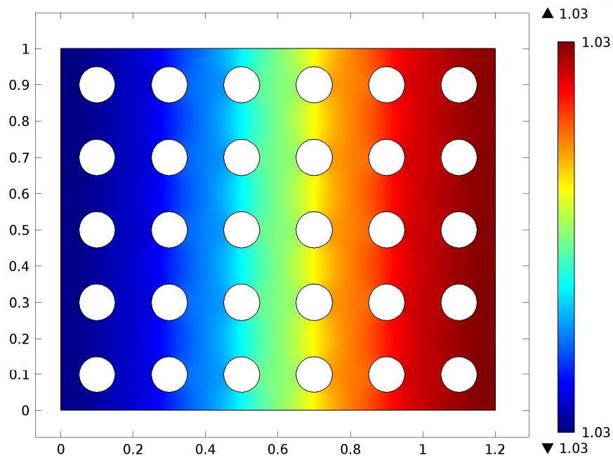
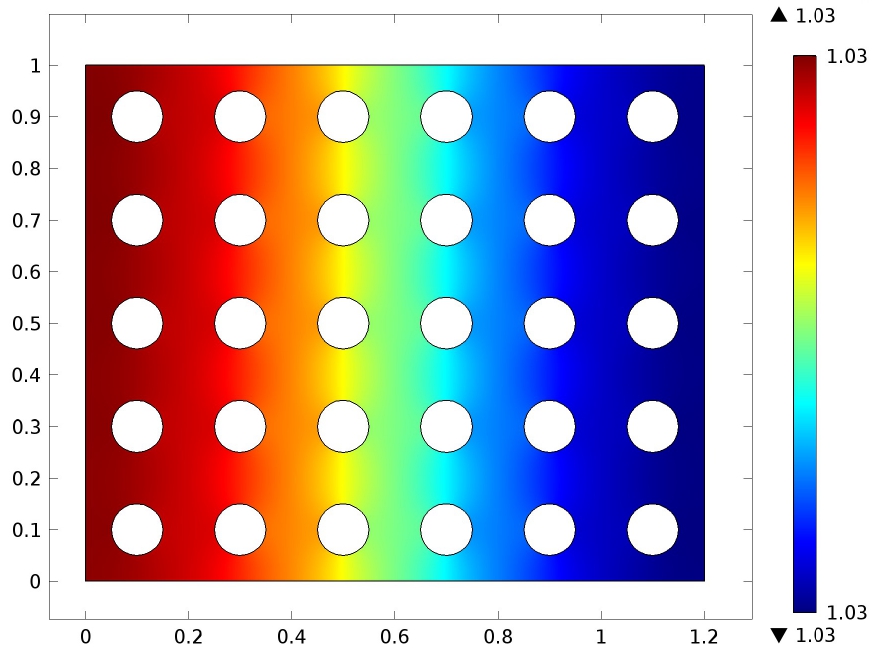
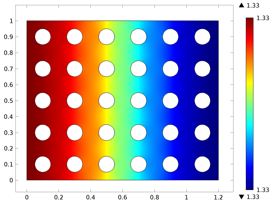
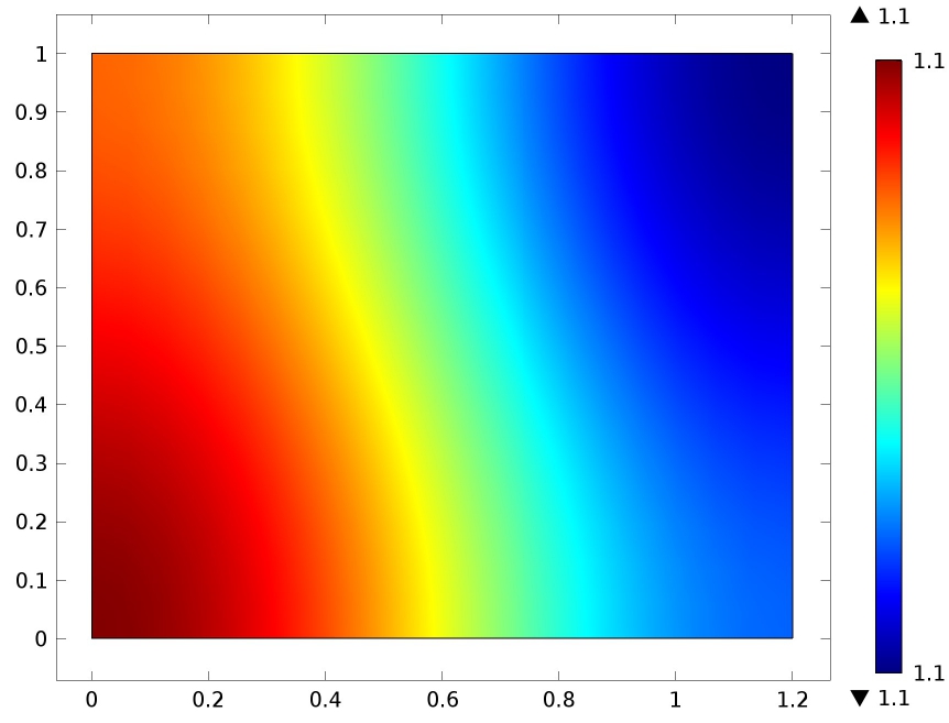
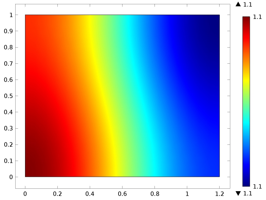
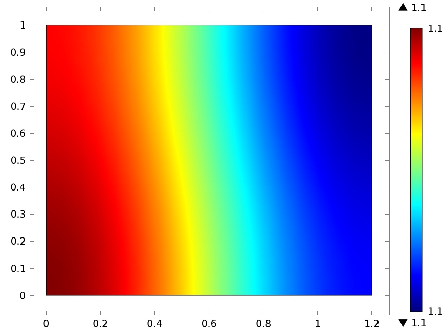
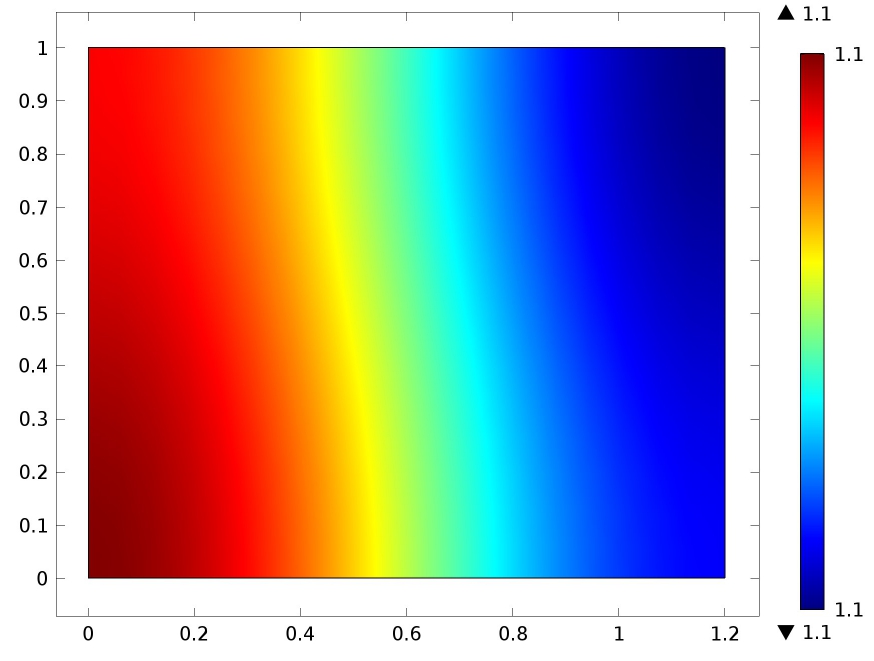
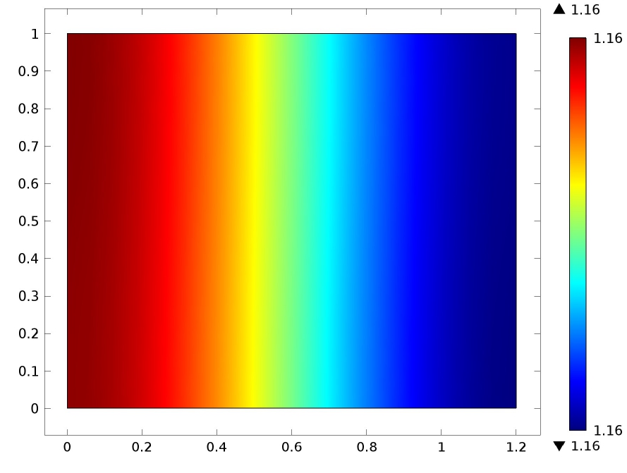
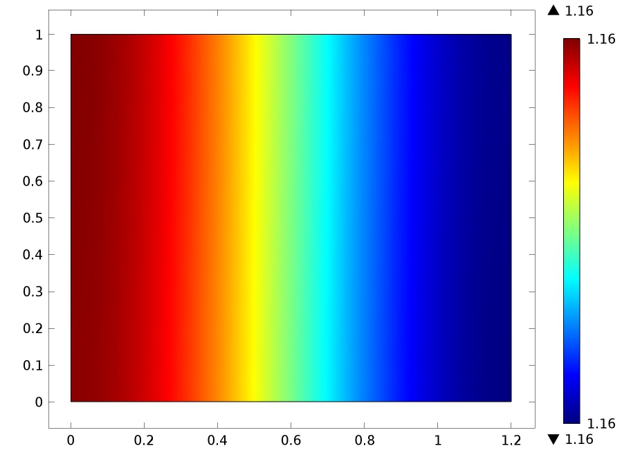
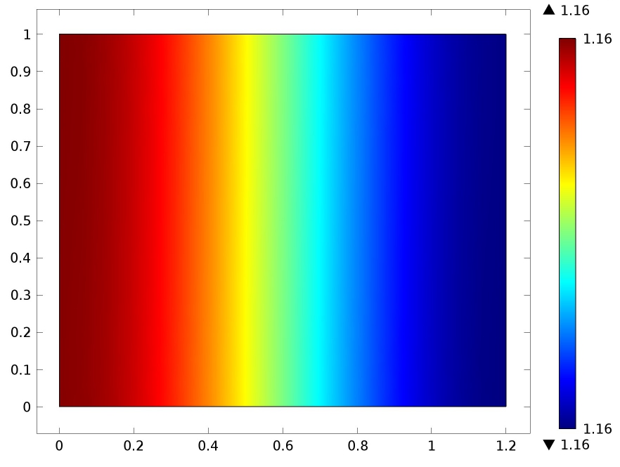
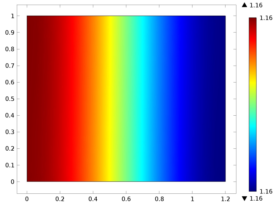
Figure 2: Concentration of the first mobile species M1subscript𝑀1M_{1} in ΩΡpsuperscriptsubscriptΞ©πœ€π‘\Omega_{\varepsilon}^{p} for different time.
Refer to caption
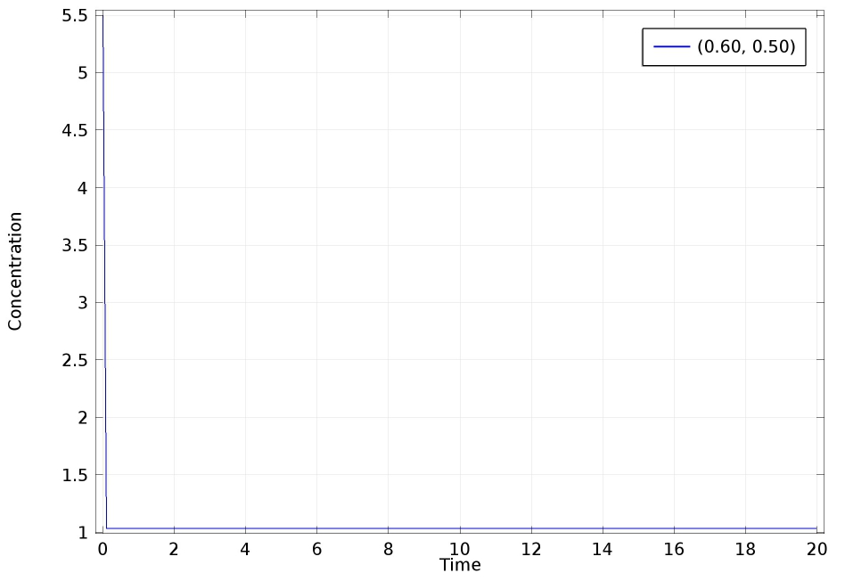
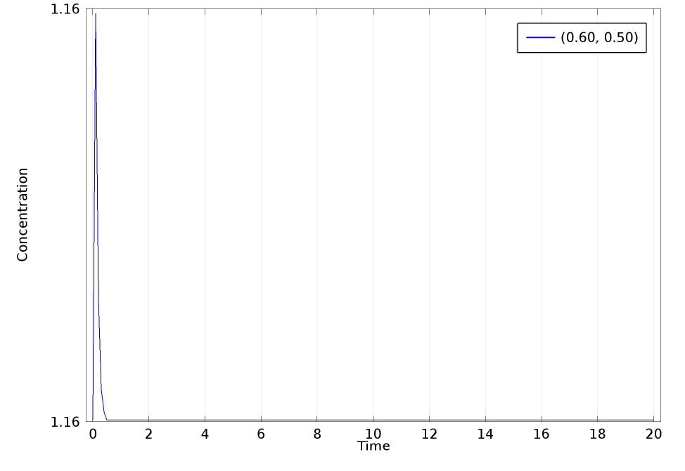
Figure 3: Concentration of M1subscript𝑀1M_{1} at the point (0.6,0.5)0.60.5(0.6,0.5) in ΩΡpsuperscriptsubscriptΞ©πœ€π‘\Omega_{\varepsilon}^{p} in 20​s20𝑠20s.

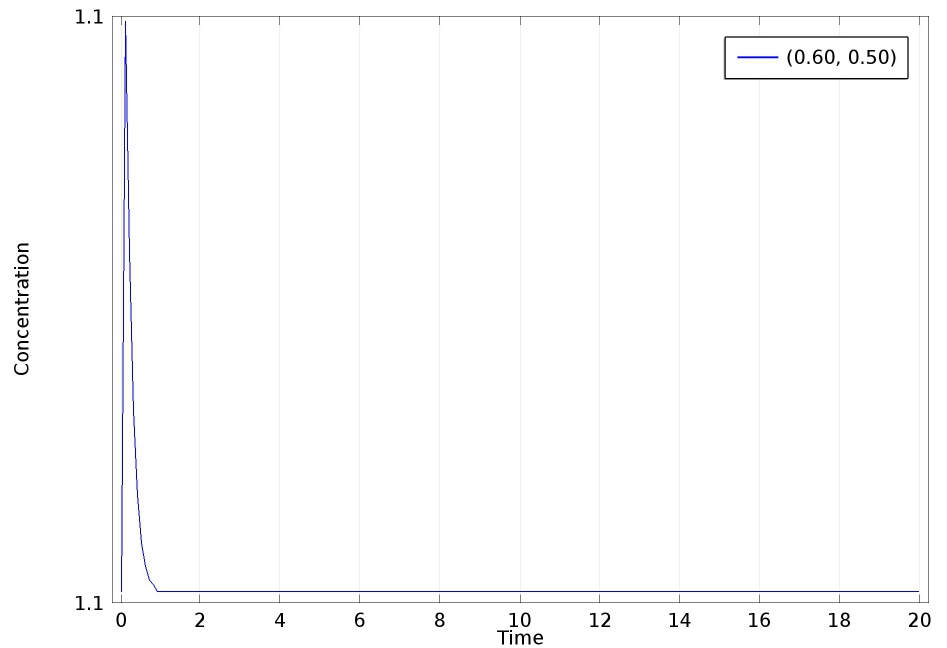
We notice that the time taken by the solver is 10​s10𝑠10s. The concentration of M1subscript𝑀1M_{1} for t=5​s,t=10​s,t=15​sformulae-sequence𝑑5𝑠formulae-sequence𝑑10𝑠𝑑15𝑠t=5s,t=10s,t=15s and t=20​s𝑑20𝑠t=20s is depicted in Figure 222. We also plotted the change of concentration of M1subscript𝑀1M_{1} at (0.6,0.5)0.60.5(0.6,0.5) for 20​s20𝑠20s in Figure 3.33. We can see that there is a jump in concentration at t=0​s𝑑0𝑠t=0s and it attains the value 5.55.55.5. Whereas at t=0.1​s𝑑0.1𝑠t=0.1s it became 1.031.031.03 so the reaction tries to stabilize it.
Refer to caption
(a)
Refer to caption
(b)
Refer to caption
(c)
Refer to caption
(d)
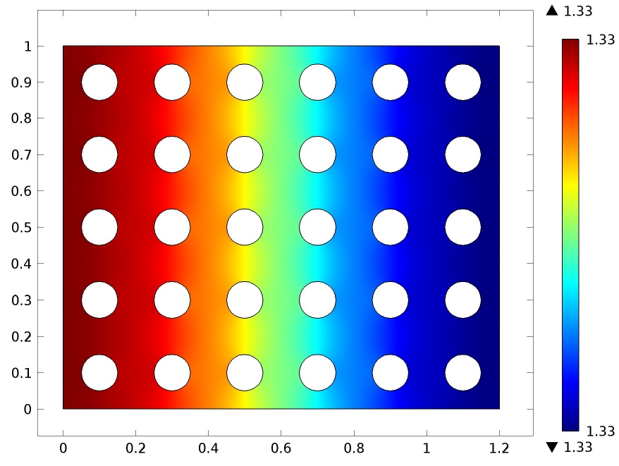
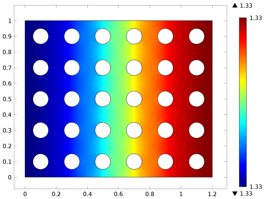
Figure 4: Concentration of the second mobile species M2subscript𝑀2M_{2} in ΩΡpsuperscriptsubscriptΞ©πœ€π‘\Omega_{\varepsilon}^{p} for different time.
Refer to caption
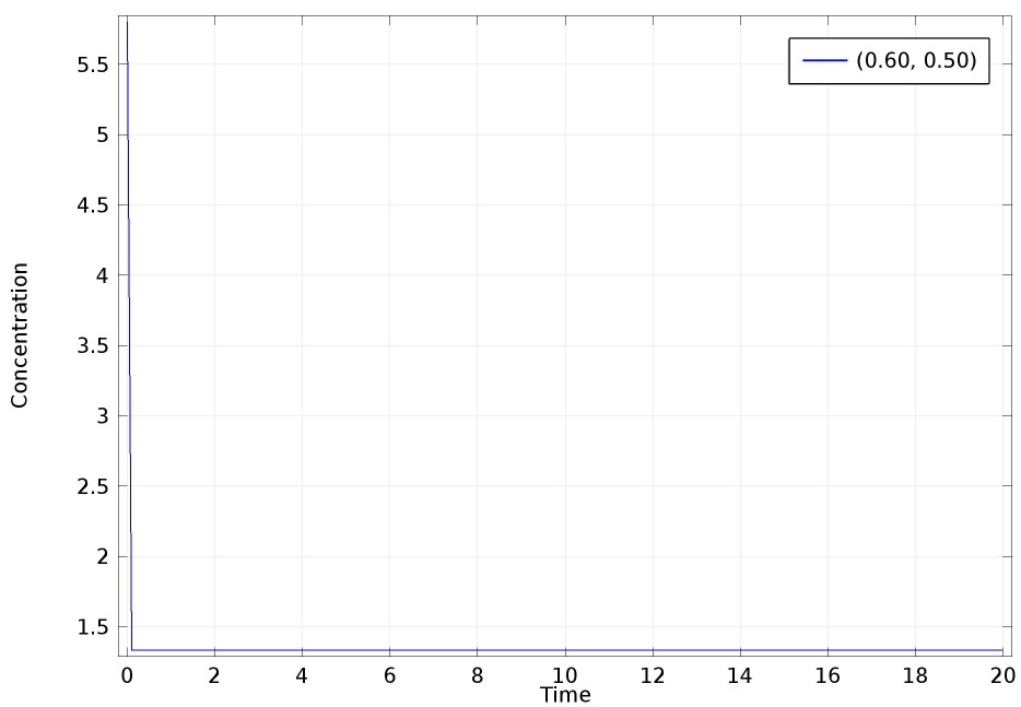
Figure 5: Concentration of M2subscript𝑀2M_{2} at the point (0.6,0.5)0.60.5(0.6,0.5) in ΩΡpsuperscriptsubscriptΞ©πœ€π‘\Omega_{\varepsilon}^{p} in 20​s20𝑠20s.

Similarly, the molar concentrations of M2subscript𝑀2M_{2} for different time is plotted in Figure 444 and the change of concentration can be seen in the Figure 555. Just like M1subscript𝑀1M_{1}, here is also a jump in the concentration at t=0​s𝑑0𝑠t=0s and the concentration became 5.85.85.8. While at t=0.1​s𝑑0.1𝑠t=0.1s it takes the value 1.331.331.33.

4.2 Solution of the Cell problems

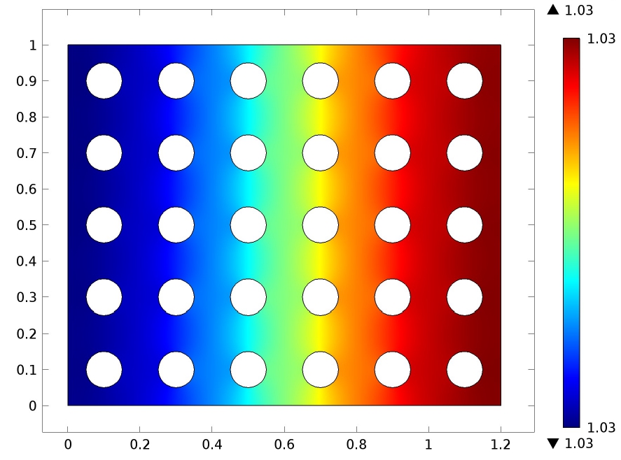
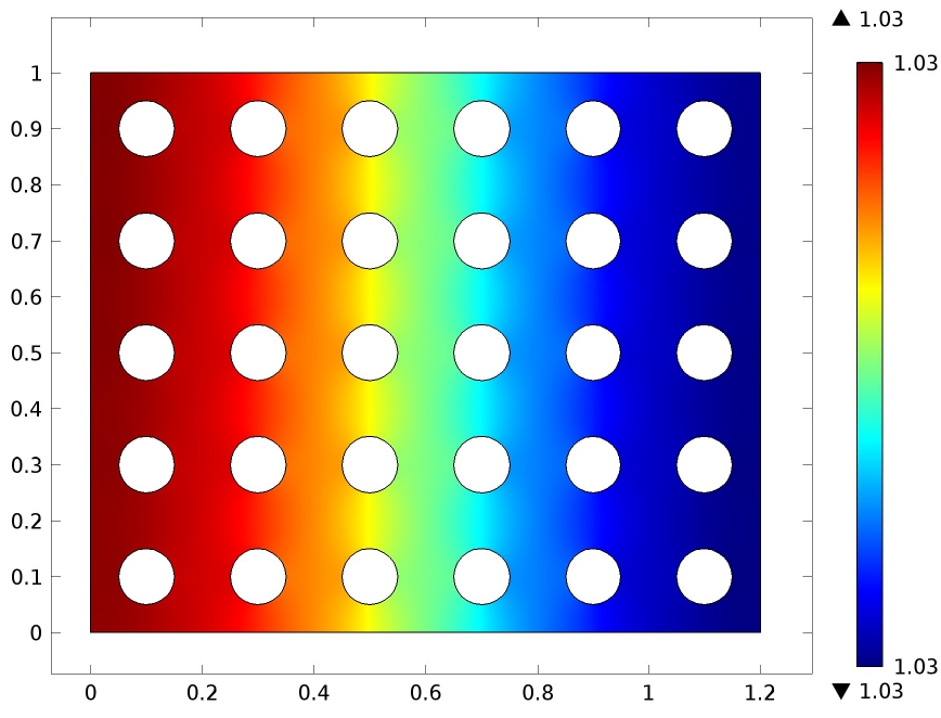
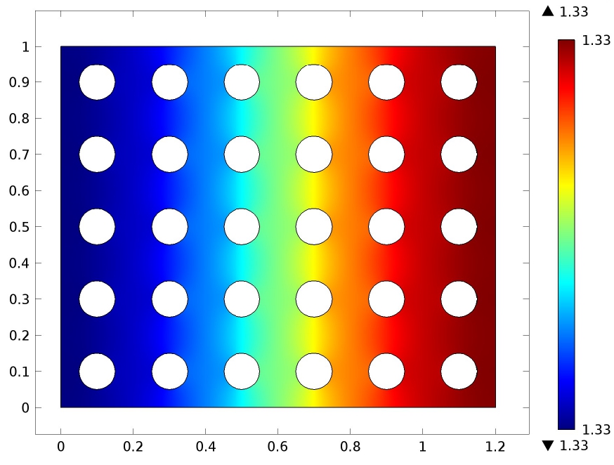
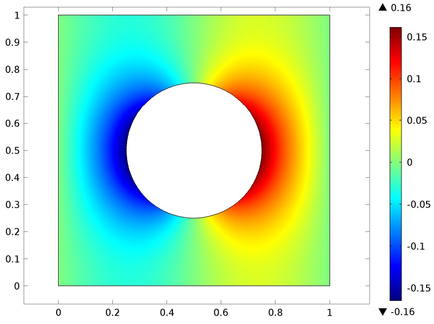
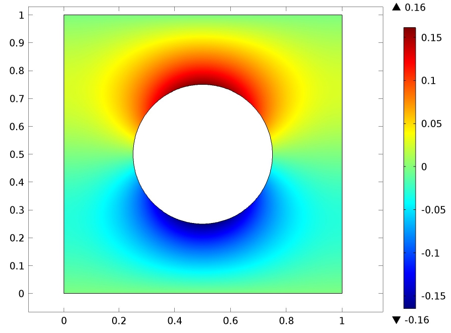
In order to simulate the upscaled equations, we need to evaluate the effective diffusion tensors for the two mobile species M1subscript𝑀1M_{1} and M2subscript𝑀2M_{2}. We commence by solving the cell problems (3.6) and the solutions is shown in Figure 666 for j=1,2𝑗12j=1,2.

Refer to caption
(a)
Refer to caption
(b)
Figure 6: Solution of the cell problems

We compute the effective tensors with the help of β€œDerived values” feature available in COMSOL. Thus we obtain

A=(ai​j)1≀i,j≀2=[0.8358βˆ’2.91316Γ—10βˆ’12βˆ’2.91334Γ—10βˆ’120.8358],𝐴subscriptsubscriptπ‘Žπ‘–π‘—formulae-sequence1𝑖𝑗2matrix0.83582.91316superscript10122.91334superscript10120.8358\displaystyle A=(a_{ij})_{1\leq i,j\leq 2}=\begin{bmatrix}0.8358&-2.91316\times 10^{-12}\\ -2.91334\times 10^{-12}&0.8358\end{bmatrix}, (4.3)
B=(bi​j)1≀i,j≀2=[1.67161βˆ’5.82632Γ—10βˆ’12βˆ’5.82667Γ—10βˆ’121.67161].𝐡subscriptsubscript𝑏𝑖𝑗formulae-sequence1𝑖𝑗2matrix1.671615.82632superscript10125.82667superscript10121.67161\displaystyle B=(b_{ij})_{1\leq i,j\leq 2}=\begin{bmatrix}1.67161&-5.82632\times 10^{-12}\\ -5.82667\times 10^{-12}&1.67161\end{bmatrix}. (4.4)

4.3 Simulation of the macromodel

We employ the idea of [25] for the simulation of the homogenized equations. We kept the same parameter values and the regularized parameter used for the micromodel as in (4.2). The effective homogenized matrices A𝐴A and B𝐡B are given by (4.3) and (4.4). Again we choose the β€œNormal” mesh to discretize the domain ΩΩ\Omega and solve the system for t=20​s𝑑20𝑠t=20s.

Refer to caption
(a)
Refer to caption
(b)
Refer to caption
(c)
Refer to caption
(d)
Figure 7: Concentration of the first mobile species M1subscript𝑀1M_{1} in ΩΩ\Omega for different time.
Refer to caption
Figure 8: Concentration of M1subscript𝑀1M_{1} at the point (0.6,0.5)0.60.5(0.6,0.5) in ΩΩ\Omega in 20​s20𝑠20s.
Refer to caption
(a)
Refer to caption
(b)
Refer to caption
(c)
Refer to caption
(d)
Figure 9: Concentration of the second mobile species M2subscript𝑀2M_{2} in ΩΩ\Omega for different time.
Refer to caption
Figure 10: Concentration of M2subscript𝑀2M_{2} at the point (0.6,0.5)0.60.5(0.6,0.5) in ΩΩ\Omega in 20​s20𝑠20s.

In this case, the time taken by the solver is 1​s1𝑠1s. We repeat the similar computation for M1subscript𝑀1M_{1} and M2subscript𝑀2M_{2} in the macro model. The results are shown in Figure 7βˆ’107107-10. However, the noticeable points are as follows: (i)𝑖(i) We use the same mesh to simulate the micro and macro system. Although the solver takes very little time to solve the macro problem in comparison to the micro problem. Hence the upscaled model is computationally efficient, (i​i)𝑖𝑖(ii) There is no such jump in concentration in the graph Figure 888 and Figure 101010. By comparing Figure 222 and 777, we can conclude that the solutions of the homogenized equations agree very well with the solutions of the original micro-scale model. It can also be understandable by comparing Figure 333 and 888. Therefore the upscaled equations describe the behavior of the microscale model very well. Thus, homogenization proved to be an efficient tool to deal with the problems arising from the microscopically heterogeneous medium.

5 Conclusion

We study crystal dissolution and precipitation in the context of a porous medium. The model takes care of the accumulation of the immobile species on the grain boundary. Using the homogenization technique, we derive the macroscopic model. In this article, we wish to understand the error caused by replacing a heterogeneous solution with a homogenization one together with numerical experiments. We observe that the macro model is advantageous for numerical simulations. Since it takes less time compared to the micromodel, it will reduce the computational cost for real-world applications. Furthermore, the numerical simulation for a test problem shows that the solution of the homogenized equation approximates the solution of the microscopic model very well. In this way, we validate the homogenization procedure and establish that it’s an efficient tool to deal with such heterogeneous problems.

References

  • [1] COMSOL Inc. http://www.comsol.com.
  • [2] Allaire, G. Homogenization and two-scale convergence. SIAM Journal on Mathematical Analysis 23, 6 (1992), 1482–1518.
  • [3] Allaire, G., Damlamian, A., and Hornung, U. Two-scale convergence on periodic structures and applications. In Proceedings of the International Conference on Mathematical Modelling of Flow through Porous Media, pp.Β 15–25.
  • [4] Cioranescu, D., Damlamian, A., Donato, P., Griso, G., and Zaki, R. The periodic unfolding method in domains with holes. SIAM Journal on Mathematical Analysis 44, 2 (2012), 718–760.
  • [5] Cioranescu, D., Damlamian, A., and Griso, G. Periodic unfolding and homogenization. Comptes Rendus Mathematique 335, 1 (2002), 99–104.
  • [6] Cioranescu, D., Damlamian, A., and Griso, G. The periodic unfolding method in homogenization. SIAM Journal on Mathematical Analysis 40, 4 (2008), 1585–1620.
  • [7] Cioranescu, D., and Donato, P. An introduction to homogenization, vol.Β 17. Oxford University Press Oxford, 1999.
  • [8] Cioranescu, D., Donato, P., and Zaki, R. The periodic unfolding method in perforated domains. Portugaliae Mathematica 63, 4 (2006).
  • [9] Cioranescu, D., and Paulin, J. S.Β J. Homogenization in open sets with holes. Journal of mathematical analysis and applications 71, 2 (1979), 590–607.
  • [10] Donato, P., and Monsurro, S. Homogenization of two heat conductors with an interfacial contact resistance. Analysis and Applications 2, 03 (2004), 247–273.
  • [11] Donato, P., and Yang, Z. The periodic unfolding method for the heat equation in perforated domains. Science China Mathematics 59, 5 (2016), 891–906.
  • [12] Ghosh, N., and Mahato, H.Β S. Diffusion-reaction-dissolution-precipitation model in a heterogeneous porous medium with nonidentical diffusion coefficients: analysis and homogenization. Accepted and to appear in Asymptotic Analysis.
  • [13] Knabner, P. A free boundary problem arising from the leaching of saine soils. SIAM Journal on Mathematical Analysis 17, 3 (1986), 610–625.
  • [14] Knabner, P., VanΒ Duijn, C., and Hengst, S. An analysis of crystal dissolution fronts in flows through porous media. part 1: Compatible boundary conditions. Advances in water resources 18, 3 (1995), 171–185.
  • [15] Lukkassen, D., Nguetseng, G., and Wall, P. Two-scale convergence. International Journal of Pure and Applied Mathematics 2, 1 (2002), 35–86.
  • [16] Mahato, H.Β S. Numerical simulations for a two-scale model in a porous medium. Numerical Analysis and Applications 10, 1 (2017), 28–36.
  • [17] Meier, S.Β A., Peter, M.Β A., Muntean, A., BΓΆhm, M., and Kropp, J. A two-scale approach to concrete carbonation. In conference; 1st International RILEM Workshop on Integral Service Life Modeling of Concrete Structures, GuimarΓ£es, Portugal; 2007-11-05; 2007-11-06 (2007), RILEM Publications, pp.Β 3–10.
  • [18] Muntean, A., and VanΒ Noorden, T.Β L. Corrector estimates for the homogenization of a locally periodic medium with areas of low and high diffusivity. European Journal of Applied Mathematics 24, 5 (2013), 657–677.
  • [19] Peter, M.Β A., and BΓΆhm, M. Scalings in homogenisation of reaction, diffusion and interfacial exchange in a two-phase medium.
  • [20] Peter, M.Β A., and BΓΆhm, M. Different choices of scaling in homogenization of diffusion and interfacial exchange in a porous medium. Mathematical Methods in the Applied Sciences 31, 11 (2008), 1257–1282.
  • [21] Peter, M.Β A., and BΓΆhm, M. Multiscale modelling of chemical degradation mechanisms in porous media with evolving microstructure. Multiscale Modeling & Simulation 7, 4 (2009), 1643–1668.
  • [22] Rubin, J. Transport of reacting solutes in porous media: Relation between mathematical nature of problem formulation and chemical nature of reactions. Water resources research 19, 5 (1983), 1231–1252.
  • [23] VanΒ Duijn, C., and Knabner, P. Crystal dissolution in porous media flow. ZEITSCHRIFT FUR ANGEWANDTE MATHEMATIK UND MECHANIK 76 (1996), 329–332.
  • [24] VanΒ Duijn, C., and Pop, I.Β S. Crystal dissolution and precipitation in porous media: pore scale analysis. Journal fΓΌr die reine und angewandte Mathematik (Crelles Journal) 2004, 577 (2004), 171–211.
  • [25] van Noorden, T.Β L. Crystal precipitation and dissolution in a porous medium: effective equations and numerical experiments. Multiscale Modeling & Simulation 7, 3 (2009), 1220–1236.
  • [26] Willis, C., and Rubin, J. Transport of reacting solutes subject to a moving dissolution boundary: Numerical methods and solutions. Water Resources Research 23, 8 (1987), 1561–1574.