Physics-Informed Neural Network Method for Parabolic Differential Equations with Sharply Perturbed Initial Conditions

Yifei Zong QiZhi He Alexandre M. Tartakovsky amt1998@illinois.edu Department of Civil and Environmental Engineering, University of Illinois Urbana-Champaign, Urbana, IL 61801 Department of Civil, Environmental, and Geo- Engineering, University of Minnesota, Minneapolis, MN 55455 Pacific Northwest National Laboratory, Richland, WA 99352.
Abstract

In this paper, we develop a physics-informed neural network (PINN) model for parabolic problems with a sharply perturbed initial condition. As an example of a parabolic problem, we consider the advection-dispersion equation (ADE) with a point (Gaussian) source initial condition. In the d𝑑d-dimensional ADE, perturbations in the initial condition decay with time t𝑑t as tβˆ’d/2superscript𝑑𝑑2t^{-d/2}, which can cause a large approximation error in the PINN solution. Localized large gradients in the ADE solution make the (common in PINN) Latin hypercube sampling of the equation’s residual highly inefficient. Finally, the PINN solution of parabolic equations is sensitive to the choice of weights in the loss function. We propose a normalized form of ADE where the initial perturbation of the solution does not decrease in amplitude and demonstrate that this normalization significantly reduces the PINN approximation error. We propose criteria for weights in the loss function that produce a more accurate PINN solution than those obtained with the weights selected via other methods. Finally, we proposed an adaptive sampling scheme that significantly reduces the PINN solution error for the same number of the sampling (residual) points. We demonstrate the accuracy of the proposed PINN model for forward, inverse, and backward ADEs.

1 Introduction

There is an increased interest in using machine learning algorithms for solving partial differential equations (PDEs). Here, we are interested in methods where the solution of a PDE is found as a global optimization problem, where the state variables are approximated with deep neural networks (DNNs) [20] or Karhunen-Loève expansion [23, 26]. One example of such methods is the physics-informed neural network (PINN) method [20, 11].

PINN is typically introduced as a method where the DNNs are trained using data and a penalty term in the form of the square of the PDE residuals evaluated at a set of residual points ( [11, 4, 3]). To facilitate this discussion, we consider the general PDE problem

ℒ​(u​(𝐱,t),𝐯​(𝐱))ℒ𝑒𝐱𝑑𝐯𝐱\displaystyle\mathcal{L}(u(\mathbf{x},t),\mathbf{v}(\mathbf{x})) =\displaystyle= 0,𝐱∈Ω,t∈[0,T]formulae-sequence0𝐱Ω𝑑0𝑇\displaystyle 0,\mathbf{x}\in\Omega,t\in[0,T] (1)
ℬ​(u​(𝐱,t),𝐯​(𝐱))ℬ𝑒𝐱𝑑𝐯𝐱\displaystyle\mathcal{B}(u(\mathbf{x},t),\mathbf{v}(\mathbf{x})) =\displaystyle= f​(𝐱,t),π±βˆˆβˆ‚Ξ©π‘“π±π‘‘π±Ξ©\displaystyle f(\mathbf{x},t),\mathbf{x}\in\partial\Omega (2)
u​(𝐱,t=tβˆ—)𝑒𝐱𝑑superscript𝑑\displaystyle u(\mathbf{x},t=t^{*}) =\displaystyle= U​(𝐱),π‘ˆπ±\displaystyle U(\mathbf{x}), (3)

where β„’β„’\mathcal{L} is a differential operator, ℬℬ\mathcal{B} is the boundary condition operator, 𝐱𝐱\mathbf{x} is the spatial coordinate vector, t𝑑t is time, ΩΩ\Omega is a bounded domain in Rnsuperscript𝑅𝑛R^{n} with the boundary βˆ‚Ξ©Ξ©\partial\Omega, u​(𝐱,t)𝑒𝐱𝑑u(\mathbf{x},t) is the state variable, 𝐯​(𝐱)𝐯𝐱\mathbf{v}(\mathbf{x}) is a vector or scalar space-dependent parameter, and U​(𝐱)π‘ˆπ±U(\mathbf{x}) is a known function. Here, we are mainly concerned with the advection-dispersion equation (ADE), where

ℒ​(u​(𝐱,t),𝐯​(𝐱))=ut+𝐩​(𝐱)β‹…βˆ‡u​(𝐱)βˆ’βˆ‡β‹…[πƒβ€‹βˆ‡u​(𝐱)],ℒ𝑒𝐱𝑑𝐯𝐱subscriptπ‘’π‘‘β‹…π©π±βˆ‡π‘’π±β‹…βˆ‡delimited-[]πƒβˆ‡π‘’π±\mathcal{L}(u(\mathbf{x},t),\mathbf{v}(\mathbf{x}))=u_{t}+\mathbf{p}(\mathbf{x})\cdot\nabla u(\mathbf{x})-\nabla\cdot[\mathbf{D}\nabla u(\mathbf{x})], (4)

𝐯​(𝐱)𝐯𝐱\mathbf{v}(\mathbf{x}) is the divergence-free velocity field, which could be given or found by solving the Darcy flow equation, and 𝐃𝐃\mathbf{D} is the dispersion coefficient. For tβˆ—=0superscript𝑑0t^{*}=0, Eq (3) provides an initial condition for the forward ADE. With tβˆ—=T>0superscript𝑑𝑇0t^{*}=T>0, Eq (3) gives a terminal condition for the backward ADE.

In the PINN method, the state variable u​(𝐱,t)𝑒𝐱𝑑u(\mathbf{x},t) is represented with a deep neural network u^​(𝐱,t;Ξ³)^𝑒𝐱𝑑𝛾\hat{u}(\mathbf{x},t;\gamma), where γ𝛾\gamma is the assembly of weights and biases of the DNN. The function u^^𝑒\hat{u} should be a (nonlinear) non-polynomial function of (𝐱,t;Ξ³)𝐱𝑑𝛾(\mathbf{x},t;\gamma), a condition that is required for a DNN with a sufficiently large size (a large γ𝛾\gamma vector) to accurately approximate any function and its derivatives [19, 1, 24]. Unlike the polynomial piece-wise representations in the finite-element (FE) methods, DNN u^​(𝐱,t;Ξ³)^𝑒𝐱𝑑𝛾\hat{u}(\mathbf{x},t;\gamma) provides a global approximation of u​(𝐱,t)𝑒𝐱𝑑u(\mathbf{x},t) in the space-time domain 𝐳=(𝐱,t)𝐳𝐱𝑑\mathbf{z}=(\mathbf{x},t), and the solution of a PDE can be found by solving a global (in time and space) residual least-square minimization problem for DNN parameters γ𝛾\gamma:

Ξ³βˆ—superscript𝛾\displaystyle\gamma^{*} =\displaystyle= arg​minΞ³[1‖Ω‖​T∫Ω∫0Tβ„’(u^(𝐱,t;Ξ³))2dtd𝐱\displaystyle\operatorname*{arg\,min}_{\gamma}\Big{[}\frac{1}{||\Omega||T}\int_{\Omega}\int_{0}^{T}\mathcal{L}(\hat{u}(\mathbf{x},t;\gamma))^{2}dtd\mathbf{x}
+\displaystyle+ 1β€–βˆ‚Ξ©β€–β€‹Tβ€‹βˆ«βˆ‚Ξ©βˆ«0T[ℬ​(u^​(𝐱,t;Ξ³))βˆ’f​(x,t)]2​𝑑t​𝑑𝐱1normΩ𝑇subscriptΞ©superscriptsubscript0𝑇superscriptdelimited-[]ℬ^𝑒𝐱𝑑𝛾𝑓π‘₯𝑑2differential-d𝑑differential-d𝐱\displaystyle\frac{1}{||\partial\Omega||T}\int_{\partial\Omega}\int_{0}^{T}[\mathcal{B}(\hat{u}(\mathbf{x},t;\gamma))-f(x,t)]^{2}dtd\mathbf{x}
+\displaystyle+ 1β€–Ξ©β€–βˆ«Ξ©[u^(𝐱,t=tβˆ—;Ξ³)βˆ’U(𝐱)]2d𝐱]\displaystyle\frac{1}{||\Omega||}\int_{\Omega}[\hat{u}(\mathbf{x},t=t^{*};\gamma)-U(\mathbf{x})]^{2}d\mathbf{x}\Big{]}

In general, the integrals in this minimization problem cannot be analytically computed due to the complexity of the DNN approximation. In the PINN method, these integrals are replaced with summations as

Ξ³βˆ—superscript𝛾\displaystyle\gamma^{*} =\displaystyle= arg​minΞ³[1NΩ​NTβˆ‘iβˆ‘jβ„’(u^(𝐱i,tj;Ξ³))2\displaystyle\operatorname*{arg\,min}_{\gamma}\Big{[}\frac{1}{N_{\Omega}N_{T}}\sum_{i}\sum_{j}\mathcal{L}(\hat{u}(\mathbf{x}_{i},t_{j};\gamma))^{2}
+\displaystyle+ 1Nβˆ‚Ξ©β€‹NTβ€‹βˆ‘iβˆ‘j[ℬ​(u^​(𝐱i,tj;Ξ³))βˆ’f​(xi,tj)]21subscript𝑁Ωsubscript𝑁𝑇subscript𝑖subscript𝑗superscriptdelimited-[]ℬ^𝑒subscript𝐱𝑖subscript𝑑𝑗𝛾𝑓subscriptπ‘₯𝑖subscript𝑑𝑗2\displaystyle\frac{1}{N_{\partial\Omega}N_{T}}\sum_{i}\sum_{j}[\mathcal{B}(\hat{u}(\mathbf{x}_{i},t_{j};\gamma))-f(x_{i},t_{j})]^{2}
+\displaystyle+ 1NΞ©βˆ‘i[u^(𝐱i,t=tβˆ—;Ξ³)βˆ’U(𝐱i)]2],\displaystyle\frac{1}{N_{\Omega}}\sum_{i}[\hat{u}(\mathbf{x}_{i},t=t^{*};\gamma)-U(\mathbf{x}_{i})]^{2}\Big{]},

where NΞ©subscript𝑁ΩN_{\Omega}, Nβˆ‚Ξ©subscript𝑁ΩN_{\partial\Omega}, and NTsubscript𝑁𝑇N_{T} are the number of points on ΩΩ\Omega, βˆ‚Ξ©Ξ©\partial\Omega, and [0,T], respectively. The summations in Eq (1) can be considered as approximations of the corresponding integrals in Eq (1) using the mid-point rule under the assumptions that the integration domains are discretized with equal-size non-overlapping subdomains and the terms in the summations are estimated in the middle of these subdomains. Alternatively, terms in the summations can be estimated at points randomly placed in the corresponding domains, in which case each term in the summations must be multiplied by a weight corresponding to the size of the volume/area associated with each discretization point. However, in the PINN literature, these conditions are usually not followed.

In the finite element least-square method (FELS), u​(𝐱,t)𝑒𝐱𝑑u(\mathbf{x},t) in Eq (1) is approximated with piecewise polynomials [18]. In the FELS method, for linear PDEs such as ADE, the integrals in Eq (1) can be computed exactly for each element in the FE discretization. In [18], the FE equations and stability analysis are presented for the forward ADE. It follows from this analysis that the FELS equations are unconditionally stable for the forward ADE and unconditionally unstable for the backward ADE. It can be shown that other FE methods as well as finite difference and finite volume schemes are also unconditionally unstable for the backward ADE. In this work, we demonstrate that the solution of the least-square problem that is based on the global DNN approximation of u𝑒u is stable under certain conditions.

The fact that the FELS formulation of linear PDEs leads to linear least-square problems is a significant advantage of this method because it guarantees a unique numerical solution of the well-posed PDE problem. On the other hand, the PINN method results in a nonlinear least-square minimization problem that might have multiple local minima. There is no guarantee that a minimization algorithm would find the global minimum even if it exists. Another challenge with nonlinear least-square minimization problems, which involve a loss function with multiple terms as in Eq (1), is that their solution might strongly depend on the weights associated with each term. To this end, a dynamic estimation of the weights during training based on the magnitude of the gradient of each term was proposed in [25]. For ADEs, an empirical relationship between the weights and Peclet number was developed in [9]. Here, we consider an alternative approach for determining weights based on the dimensionless analysis of the ADE.

For some initial and boundary conditions, the range/amplitude of the solutions of parabolic equations such as the ADE can change over time by several orders of magnitude. Global approximations of such solutions in the space-time domain with a finite-size DNN might be challenging. To illustrate this point, we use a DNN to approximate the function

u​(x,t)=12​π​(Ξ΅2+2​D​t)​exp⁑(βˆ’(xβˆ’x0βˆ’v​t)22​(Ξ΅2+2​D​t)),𝑒π‘₯𝑑12πœ‹superscriptπœ€22𝐷𝑑superscriptπ‘₯subscriptπ‘₯0𝑣𝑑22superscriptπœ€22𝐷𝑑u(x,t)=\frac{1}{\sqrt{2\pi(\varepsilon^{2}+2Dt)}}\exp\Big{(}-\frac{(x-x_{0}-vt)^{2}}{2(\varepsilon^{2}+2Dt)}\Big{)}, (7)

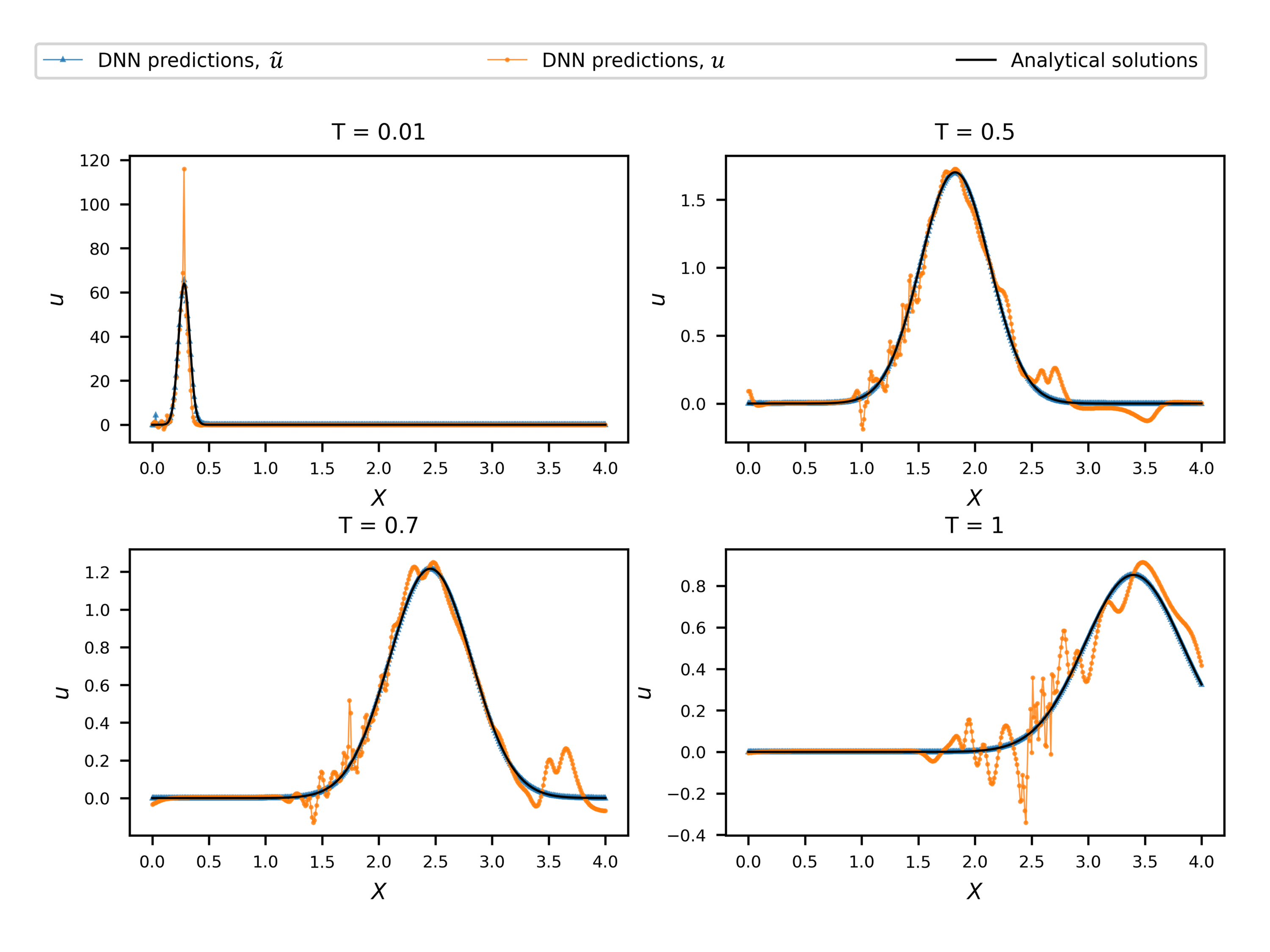
which is the solution of the one-dimensional ADE with the Gaussian source initial condition u​(x,t=0)=12​π​Ρ2​exp⁑(βˆ’(xβˆ’x0)22​Ρ2)𝑒π‘₯𝑑012πœ‹superscriptπœ€2superscriptπ‘₯subscriptπ‘₯022superscriptπœ€2u(x,t=0)=\frac{1}{\sqrt{2\pi\varepsilon^{2}}}\exp\Big{(}-\frac{(x-x_{0})^{2}}{2\varepsilon^{2}}\Big{)} (Ξ΅πœ€\varepsilon and x0subscriptπ‘₯0x_{0} are the spread and center of the source, respectively) and the homogeneous Dirichlet BC at ±∞plus-or-minus\pm\infty. Other parameters in Eq (7) are the advection velocity v𝑣v and the dispersion coefficient D𝐷D. According to Eq (7), the maximum value of u​(x,t)𝑒π‘₯𝑑u(x,t) decays as um​a​x​(t)=12​π​(Ξ΅2+2​D​t)subscriptπ‘’π‘šπ‘Žπ‘₯𝑑12πœ‹superscriptπœ€22𝐷𝑑u_{max}(t)=\frac{1}{\sqrt{2\pi(\varepsilon^{2}+2Dt)}}, while the minimum of u​(x,t)𝑒π‘₯𝑑u(x,t) is bounded by 0. Here, we set Ξ΅=0.025πœ€0.025\varepsilon=0.025, x0=0.25subscriptπ‘₯00.25x_{0}=0.25, D=0.093𝐷0.093D=0.093, and v=3.15𝑣3.15v=3.15, and approximate u​(x,t)𝑒π‘₯𝑑u(x,t) in the space-time domain [0,4]Γ—[0,1]0401[0,4]\times[0,1]. We set the DNN size to five hidden layers and 60 neurons per layer and train it using samples of u​(x,t)𝑒π‘₯𝑑u(x,t) on the 201Γ—101201101201\times 101 uniform mesh in the xβˆ’tπ‘₯𝑑x-t space.

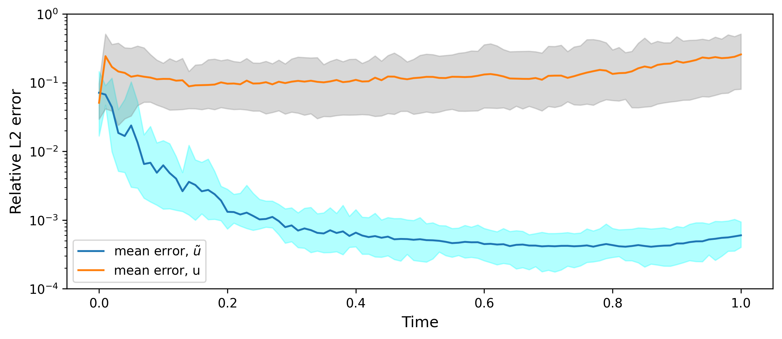
Figure 1 shows u​(x,t)𝑒π‘₯𝑑u(x,t) and its DNN approximation u^​(x,t,Ξ³)^𝑒π‘₯𝑑𝛾\hat{u}(x,t,\gamma), which is trained (i.e., the DNN parameters γ𝛾\gamma are estimated) using u𝑒u samples. It can be seen that the DNN develops oscillations and, in general, is doing a poor job at approximating u​(x,t)𝑒π‘₯𝑑u(x,t) at all times. Next, we normalize u​(x,t)𝑒π‘₯𝑑u(x,t) as u~​(x,t)=u​(x,t)um​a​x​(t)~𝑒π‘₯𝑑𝑒π‘₯𝑑subscriptπ‘’π‘šπ‘Žπ‘₯𝑑\tilde{u}(x,t)=\frac{u(x,t)}{u_{max}(t)} such that the maximum and minimum of the normalized function are 1 and 0 at all times. Then, we approximate u​(x,t)𝑒π‘₯𝑑{u}(x,t) as u​(x,t)β‰ˆu~^​(x,t,Ξ³~)​um​a​x​(t)𝑒π‘₯𝑑^~𝑒π‘₯𝑑~𝛾subscriptπ‘’π‘šπ‘Žπ‘₯𝑑{u}(x,t)\approx\hat{\tilde{u}}(x,t,\tilde{\gamma})u_{max}(t), where u~^​(x,t,Ξ³~)^~𝑒π‘₯𝑑~𝛾\hat{\tilde{u}}(x,t,\tilde{\gamma}) is a DNN (with the parameters Ξ³~~𝛾\tilde{\gamma}) that is trained using the samples of u~​(x,t)~𝑒π‘₯𝑑\tilde{u}(x,t). We set u~^​(x,t,Ξ³~)^~𝑒π‘₯𝑑~𝛾\hat{\tilde{u}}(x,t,\tilde{\gamma}) to have the same size as u^​(x,t,Ξ³)^𝑒π‘₯𝑑𝛾\hat{{u}}(x,t,\gamma) and train it with the same number of samples. Figure 1 shows that u~^​(x,t)^~𝑒π‘₯𝑑\hat{\tilde{u}}(x,t) provides a significantly more accurate approximation of u𝑒u than u^​(x,t)^𝑒π‘₯𝑑\hat{u}(x,t). The DNN training is a nonlinear least-square minimization problem, whose solution (the values of the DNN’s weights) can depend on the initialization of the minimization problem [6, 14]. Figure 2 shows the average relative L2 errors in the approximations of u​(x,t)𝑒π‘₯𝑑u(x,t) obtained with the samples of u​(x,t)𝑒π‘₯𝑑u(x,t) and u~​(x,t)~𝑒π‘₯𝑑\tilde{u}(x,t) as functions of time found from six different random initializations of the DNN weights. This figure also presents the range of errors (the shaded areas) corresponding to the different DNN weights initializations. At t=0𝑑0t=0, u~​(x,t)=u​(x,t)~𝑒π‘₯𝑑𝑒π‘₯𝑑\tilde{u}(x,t)={u}(x,t), and the L2 errors in the two approximations are approximately the same. However, for the approximation u​(x,t)β‰ˆu~^​(x,t,Ξ³~)​um​a​x​(t)𝑒π‘₯𝑑^~𝑒π‘₯𝑑~𝛾subscriptπ‘’π‘šπ‘Žπ‘₯𝑑u(x,t)\approx\hat{\tilde{u}}(x,t,\tilde{\gamma})u_{max}(t), the L2 error at t=0𝑑0t=0 is the largest and decreases with time by more than two orders of magnitude. This is because the gradient of u~​(x,t)~𝑒π‘₯𝑑\tilde{u}(x,t) with respect to (x,t)π‘₯𝑑(x,t) (the rate of change in space and time) is largest at t=0𝑑0t=0 and decreases with time. This is not the case for the approximation based on u​(x,t)β‰ˆu^​(x,t,Ξ³)𝑒π‘₯𝑑^𝑒π‘₯𝑑𝛾u(x,t)\approx\hat{u}(x,t,\gamma)–its L2 error is smallest at t=0𝑑0t=0 and increases with time by one order of magnitude. Also, Figure 2 shows that the standard deviation of L2 error in the approximation u~^​(x,t)​um​a​x​(t)^~𝑒π‘₯𝑑subscriptπ‘’π‘šπ‘Žπ‘₯𝑑\hat{\tilde{u}}(x,t)u_{max}(t) is two orders of magnitude smaller than that in the u^​(x,t)^𝑒π‘₯𝑑\hat{u}(x,t) approximation, i.e., a DNN approximation of u~​(x,t)~𝑒π‘₯𝑑\tilde{u}(x,t) is significantly less sensitive to initialization than that of u​(x,t)𝑒π‘₯𝑑{u}(x,t). We note that the normalization of u​(x,t)𝑒π‘₯𝑑u(x,t) with the constant um​a​x​(t=0)subscriptπ‘’π‘šπ‘Žπ‘₯𝑑0u_{max}(t=0), while making the normalized function to be in the [0,1] range at all times, does not significantly improve the DNN approximation of u​(x,t)𝑒π‘₯𝑑u(x,t).

The convergence of the PINN method with the number of collocation points was proven for elliptic and parabolic PDEs, given that the DNN is large enough to accurately represent the solution [21]. The results in Figures 1 and 2 show that for certain initial conditions, a non-trivial normalization (i.e., normalization with a time-dependent factor rather than a constant) is required to allow an accurate representation with a DNN of a relatively small size.

Later in this work, we demonstrate that the PINN method fails in obtaining an accurate solution of the two-dimensional ADE (4) with a similar Gaussian source initial condition. Also, we demonstrate that the accuracy of the PINN method can be significantly improved by reformulating the ADE equation such that the maximum of the solution stays near 1 at all times.
Refer to caption
Figure 1: The reference function u​(x,t)𝑒π‘₯𝑑u(x,t) and the DNN approximations u​(x,t)β‰ˆu~^​(x,t,Ξ³~)​um​a​x​(t)𝑒π‘₯𝑑^~𝑒π‘₯𝑑~𝛾subscriptπ‘’π‘šπ‘Žπ‘₯𝑑u(x,t)\approx\hat{\tilde{u}}(x,t,\tilde{\gamma})u_{max}(t) and u^​(x,t,Ξ³)^𝑒π‘₯𝑑𝛾\hat{u}(x,t,\gamma) versus xπ‘₯x at t=0.01𝑑0.01t=0.01, 0.5, 0.7, and 1.
Refer to caption
Figure 2: Average relative L2 error in the DNN approximations of u​(x,t)𝑒π‘₯𝑑u(x,t) obtained with the u𝑒u and normalized u~~𝑒\tilde{u} data obtained using six random initializations of the DNN weights. The upper and lower bounds of the shaded areas correspond to the maximum and minimum errors in the approximations obtained with the six DNN weight initializations.

Even when an accurate DNN representation is available, the number of the residual points required for obtaining an accurate solution can be prohibitively large. The common practice is to place residual points uniformly or randomly using Latin hypercube sampling (LHS) [20, 22, 10]. The latter was found to require less residual points to achieve the same accuracy as in the case with uniformly placed residual points. However, for hyperbolic or advection-dominated parabolic problems, the LHS placement of residual points can be inadequate. In [17], it was proposed to place the residual points adaptively according to the magnitude of the PDE residuals. Here, we propose an alternative strategy for identifying the locations of the residual points that is based on the rate of change of the solution.

Despite the above-mentioned challenges, multiple studies demonstrated that the PINN method with a sufficient number of collocation points can obtain accurate solutions of both linear and nonlinear PDEs. For example, PINN was used to solve a linear diffusion equation with a space-dependent diffusion coefficient describing saturated flow in porous media and a nonlinear diffusion equation describing flow in unsaturated porous media [22]. In [8], PINN was used to solve a joint inverse problem for a system of advection-diffusion and diffusion (flow) equations describing flow and transport in porous media. In [9], some advantages of PINN over the FE method were demonstrated for a forward ADE with the direction of the advection velocity 𝐯𝐯\mathbf{v} being different from the grid orientation.

We note that a comparative study of PINN with FE or other numerical methods is not the goal of this work. Our main arguments for using PINN are the backward ADE and inverse ADE problem where the unknown parameter is the hydraulic conductivity in the Darcy flow equation for the velocity 𝐯​(x)𝐯π‘₯\mathbf{v}(x) in Eq (4). In the former case, most methods based on piece-wise continuous approximations fail. In the latter case, the standard inverse methods such as the maximum a posteriori (MAP) method suffer from the curse of dimensionality because its cost scales as N3superscript𝑁3N^{3}, where N𝑁N is the number of unknown parameters [26]. Therefore, the main focus of this work is on the backward and inverse ADE problems. However, the ability of a method to accurately solve a forward ADE is a necessary condition for that method to be successful in solving inverse and backward ADEs. The proposed modifications of the PINN method improve its accuracy for the forward ADE and make it possible to apply PINN for the inverse and backward ADEs.

This paper is organized as follows. In Section 2, we demonstrate how the PINN method can fail for the forward ADE with an instantaneous Gaussian source. We show that using either learning rate annealing [25] or different combinations of fixed weights does not produce an accurate solution. In Section 3, we propose the normalized formulation of ADE, estimates of the weights in the PINN loss function, and the adaptive sampling scheme for residual points. In Section 4, we present forward and inverse PINN solutions of the normalized ADEs. We demonstrate that the assimilation of state measurements in the PINN model improves the estimations of both the state variable and parameters. In Section 5, we discuss the PINN solutions of the backward normalized ADE equation. Conclusions are given in Section 6.

2 PINN formulation for the advection-dispersion equation

2.1 Problem statement

We consider the two-dimensional non-reactive solute transport of a scalar field u​(𝐱,t)𝑒𝐱𝑑u(\mathbf{x},t) in a non-uniform flow field in a fully saturated heterogeneous porous media with space-dependent conductivity K​(𝒙)𝐾𝒙K(\bm{x}).

The evolution of u​(𝐱,t)𝑒𝐱𝑑u(\mathbf{x},t) is governed by the ADE:

ut+βˆ‡β‹…[𝐯​(𝐱)​u​(𝐱)]=βˆ‡β‹…[πƒβ€‹βˆ‡u​(𝐱)],𝐱∈Ω,t∈(0,T)u​(𝐱,t)=gd​(𝐱),x1=0βˆ‚u​(𝐱,t)/βˆ‚x1=gn​(𝐱),x1=L1βˆ‚u​(𝐱,t)/βˆ‚x2=gn​(𝐱),x2=0andx2=L2subscriptπ‘’π‘‘β‹…βˆ‡delimited-[]𝐯𝐱𝑒𝐱formulae-sequenceabsentβ‹…βˆ‡delimited-[]πƒβˆ‡π‘’π±formulae-sequence𝐱Ω𝑑0𝑇𝑒𝐱𝑑formulae-sequenceabsentsubscript𝑔𝑑𝐱subscriptπ‘₯10𝑒𝐱𝑑subscriptπ‘₯1formulae-sequenceabsentsubscript𝑔𝑛𝐱subscriptπ‘₯1subscript𝐿1𝑒𝐱𝑑subscriptπ‘₯2formulae-sequenceabsentsubscript𝑔𝑛𝐱formulae-sequencesubscriptπ‘₯20andsubscriptπ‘₯2subscript𝐿2\begin{array}[]{ll}u_{t}+\nabla\cdot[{\mathbf{v}}(\mathbf{x})u(\mathbf{x})]&=\nabla\cdot[\mathbf{D}\nabla u(\mathbf{x})],\quad\mathbf{x}\in\Omega,\quad t\in(0,T)\\ u(\mathbf{x},t)&=g_{d}(\mathbf{x}),\quad\quad x_{1}=0\\ \partial u(\mathbf{x},t)/\partial x_{1}&=g_{n}(\mathbf{x}),\quad\quad x_{1}=L_{1}\\ \partial u(\mathbf{x},t)/\partial x_{2}&=g_{n}(\mathbf{x}),\quad\quad x_{2}=0\quad{\rm{and}}\quad x_{2}=L_{2}\end{array} (8)

For the forward ADE, we assume the initial condition

u​(x,t=0)=M2​π​Ρ2​exp⁑[βˆ’(x1βˆ’x1βˆ—)2+(x2βˆ’x2βˆ—)22​Ρ2],𝐱∈Ωformulae-sequence𝑒π‘₯𝑑0𝑀2πœ‹superscriptπœ€2superscriptsubscriptπ‘₯1superscriptsubscriptπ‘₯12superscriptsubscriptπ‘₯2superscriptsubscriptπ‘₯222superscriptπœ€2𝐱Ωu(x,t=0)=\frac{M}{2\pi\varepsilon^{2}}\exp\left[-\frac{(x_{1}-x_{1}^{*})^{2}+(x_{2}-x_{2}^{*})^{2}}{2\varepsilon^{2}}\right],\quad\mathbf{x}\in\Omega (9)

which describes a Gaussian source centered at (x1βˆ—,x2βˆ—)superscriptsubscriptπ‘₯1superscriptsubscriptπ‘₯2(x_{1}^{*},x_{2}^{*}) with the total mass M𝑀M and standard deviation Ξ΅πœ€\varepsilon. For the backward ADE, u​(𝐱)𝑒𝐱u(\mathbf{x}) is known at the terminal time T>0𝑇0T>0:

u​(𝐱,t=T)=U​(𝐱),𝐱∈Ω,formulae-sequenceπ‘’π±π‘‘π‘‡π‘ˆπ±π±Ξ©u(\mathbf{x},t=T)=U(\mathbf{x}),\quad\mathbf{x}\in\Omega, (10)

where U​(x)π‘ˆπ‘₯U(x) is the (known) terminal condition. For both, the forward and inverse problems, we assume the homogeneous Direchlet and Neumann boundary conditions, i.e., gd​(𝐱)=gd​(𝐱)=0subscript𝑔𝑑𝐱subscript𝑔𝑑𝐱0g_{d}(\mathbf{x})=g_{d}(\mathbf{x})=0.

The dispersion tensor 𝐃𝐃\mathbf{D} is defined as (Bear, 1972):

Dx​x=Dw+aL​v12β€–vβ€–+aT​v22β€–vβ€–Dy​y=Dw+aL​v22β€–vβ€–+aT​v12β€–vβ€–Dx​y=Dy​x=Dw+(aLβˆ’aT)​v1​v2β€–vβ€–,subscript𝐷π‘₯π‘₯subscript𝐷𝑀subscriptπ‘ŽπΏsuperscriptsubscript𝑣12norm𝑣subscriptπ‘Žπ‘‡superscriptsubscript𝑣22norm𝑣subscript𝐷𝑦𝑦subscript𝐷𝑀subscriptπ‘ŽπΏsuperscriptsubscript𝑣22norm𝑣subscriptπ‘Žπ‘‡superscriptsubscript𝑣12norm𝑣subscript𝐷π‘₯𝑦subscript𝐷𝑦π‘₯subscript𝐷𝑀subscriptπ‘ŽπΏsubscriptπ‘Žπ‘‡subscript𝑣1subscript𝑣2norm𝑣\begin{split}D_{xx}=D_{w}+a_{L}\frac{{v_{1}}^{2}}{\|v\|}+a_{T}\frac{{v_{2}}^{2}}{\|v\|}\\ D_{yy}=D_{w}+a_{L}\frac{{v_{2}}^{2}}{\|v\|}+a_{T}\frac{{v_{1}}^{2}}{\|v\|}\\ D_{xy}=D_{yx}=D_{w}+(a_{L}-a_{T})\frac{v_{1}v_{2}}{\|v\|},\end{split} (11)

where 𝐯​(𝐱)𝐯𝐱\mathbf{v}(\mathbf{x}) is the advection velocity given by the Darcy law:

𝐯​(𝐱)=βˆ’K​(𝐱)Ο•β€‹βˆ‡h​(𝐱),𝐯𝐱𝐾𝐱italic-Ο•βˆ‡β„Žπ±\mathbf{v}(\mathbf{x})=-\frac{K(\mathbf{x})}{\phi}\nabla h(\mathbf{x}), (12)

where Ο•italic-Ο•\phi is the known porosity and hβ„Žh is the hydraulic conductivity given by the Darcy flow equation:

βˆ‡β‹…[K​(𝐱)β€‹βˆ‡h​(𝐱)]=0,𝐱∈Ωh​(𝐱)=H,x1=L1βˆ’K​(𝐱)β€‹βˆ‚h​(𝐱)/βˆ‚x1=q,x1=0βˆ’K​(𝐱)β€‹βˆ‚h​(𝐱)/βˆ‚x2=0,x2=0​and​x2=L2.\begin{array}[]{ll}\begin{split}\nabla\cdot\left[K(\mathbf{x})\nabla h(\mathbf{x})\right]&=0,\quad\mathbf{x}\in\Omega\\ h(\mathbf{x})&={H},\quad{x_{1}}=L_{1}\\ -K(\mathbf{x})\partial h(\mathbf{x})/\partial x_{1}&=q,\quad x_{1}=0\\ -K(\mathbf{x})\partial h(\mathbf{x})/\partial x_{2}&=0,\quad x_{2}=0\>{\rm{and}}\>x_{2}=L_{2}.\end{split}\end{array} (13)

Here, H𝐻H and qπ‘žq are the known head and flux at the Dirichlet and Neumann boundary conditions, respectively. We generate Y​(𝐱)=ln⁑K​(𝐱)π‘Œπ±πΎπ±Y(\mathbf{x})=\ln K(\mathbf{x}) as a realization of a Gaussian random field with the constant mean and covariance function c​o​v​(x,xβ€²)=ΟƒY2​exp⁑(β€–xβˆ’xβ€²β€–2Ξ»2)π‘π‘œπ‘£π‘₯superscriptπ‘₯β€²subscriptsuperscript𝜎2π‘Œsuperscriptnormπ‘₯superscriptπ‘₯β€²2superscriptπœ†2cov(x,x^{\prime})=\sigma^{2}_{Y}\exp(\frac{{\|x-x^{\prime}\|}^{2}}{\lambda^{2}}), where ΟƒY2subscriptsuperscript𝜎2π‘Œ\sigma^{2}_{Y} is the variance of and Ξ»πœ†\lambda is the correlation length.

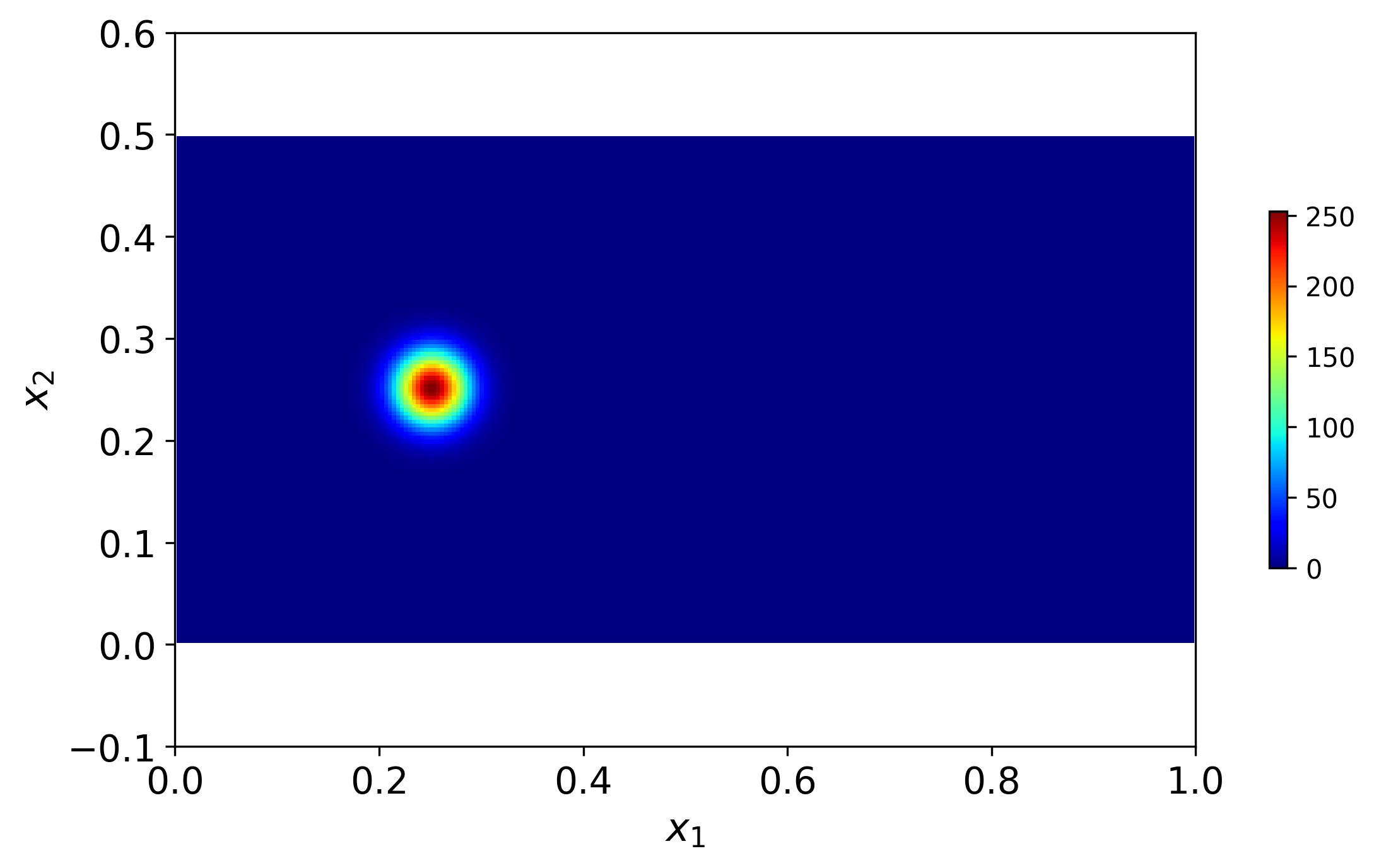
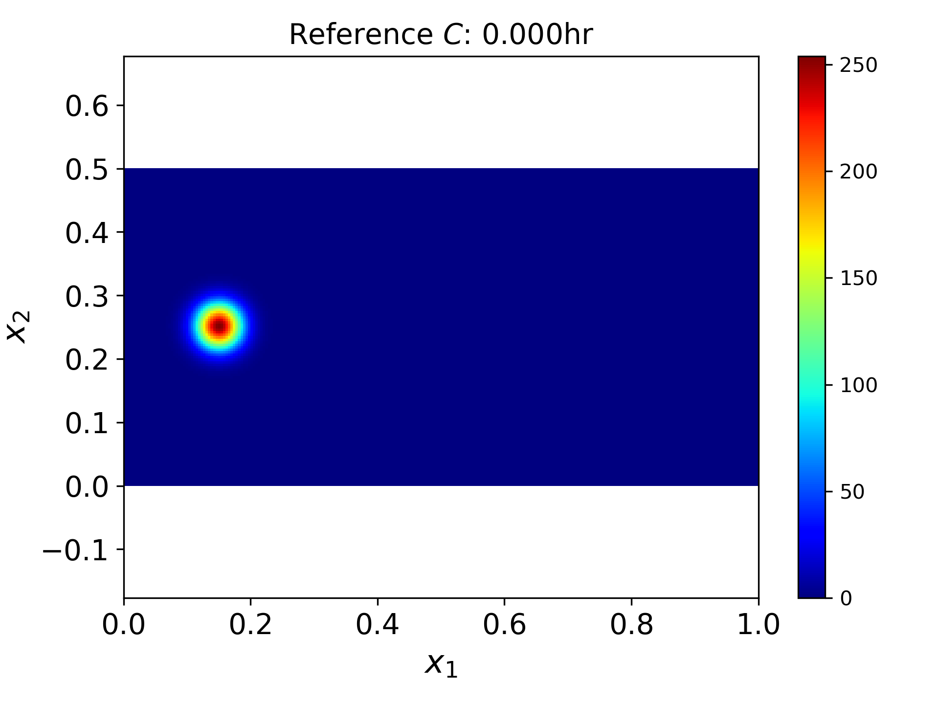
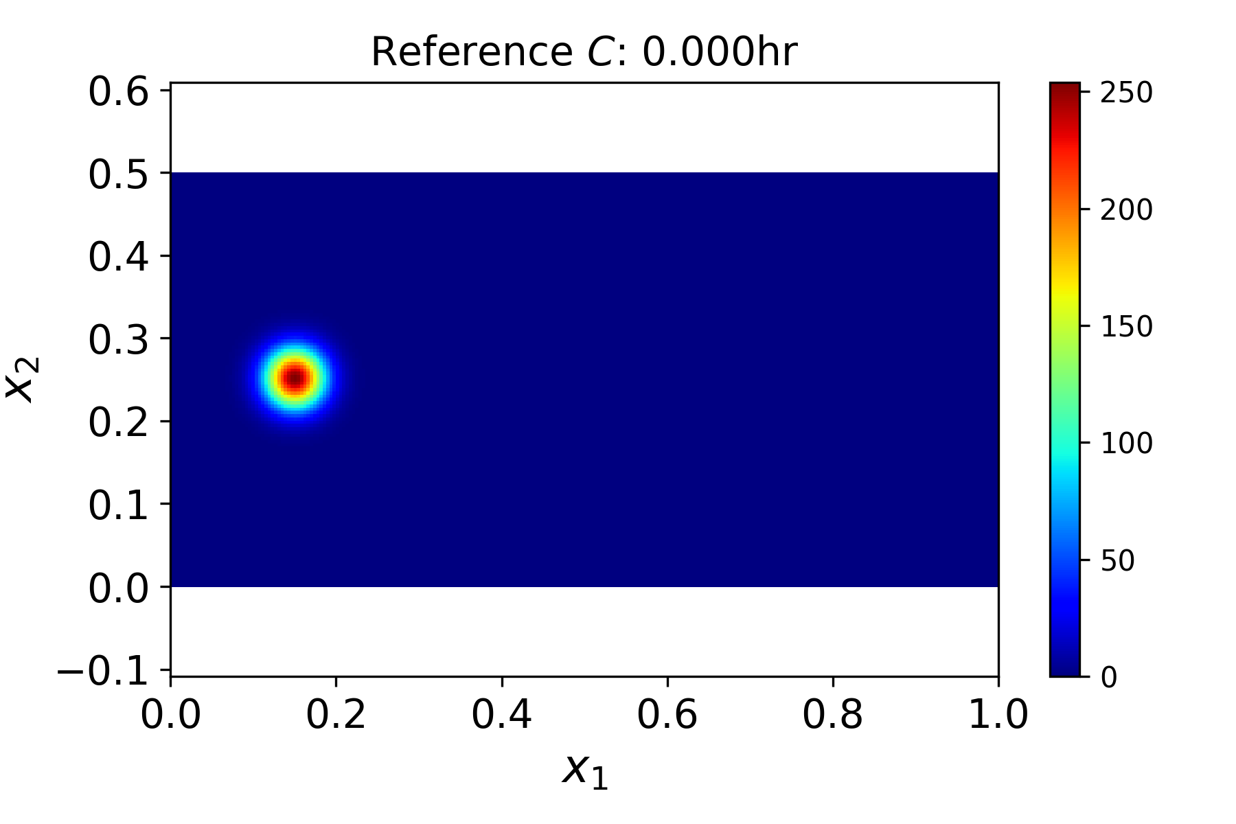
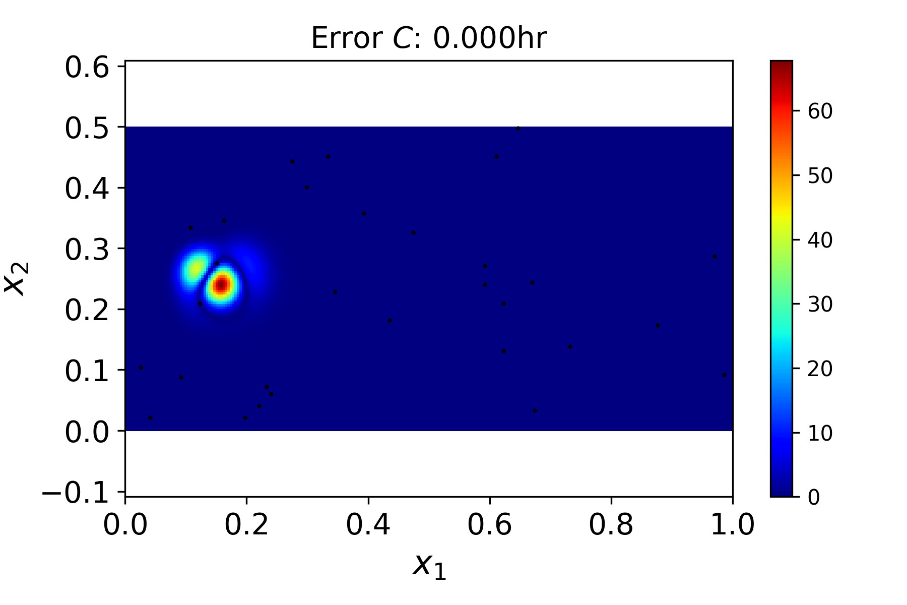
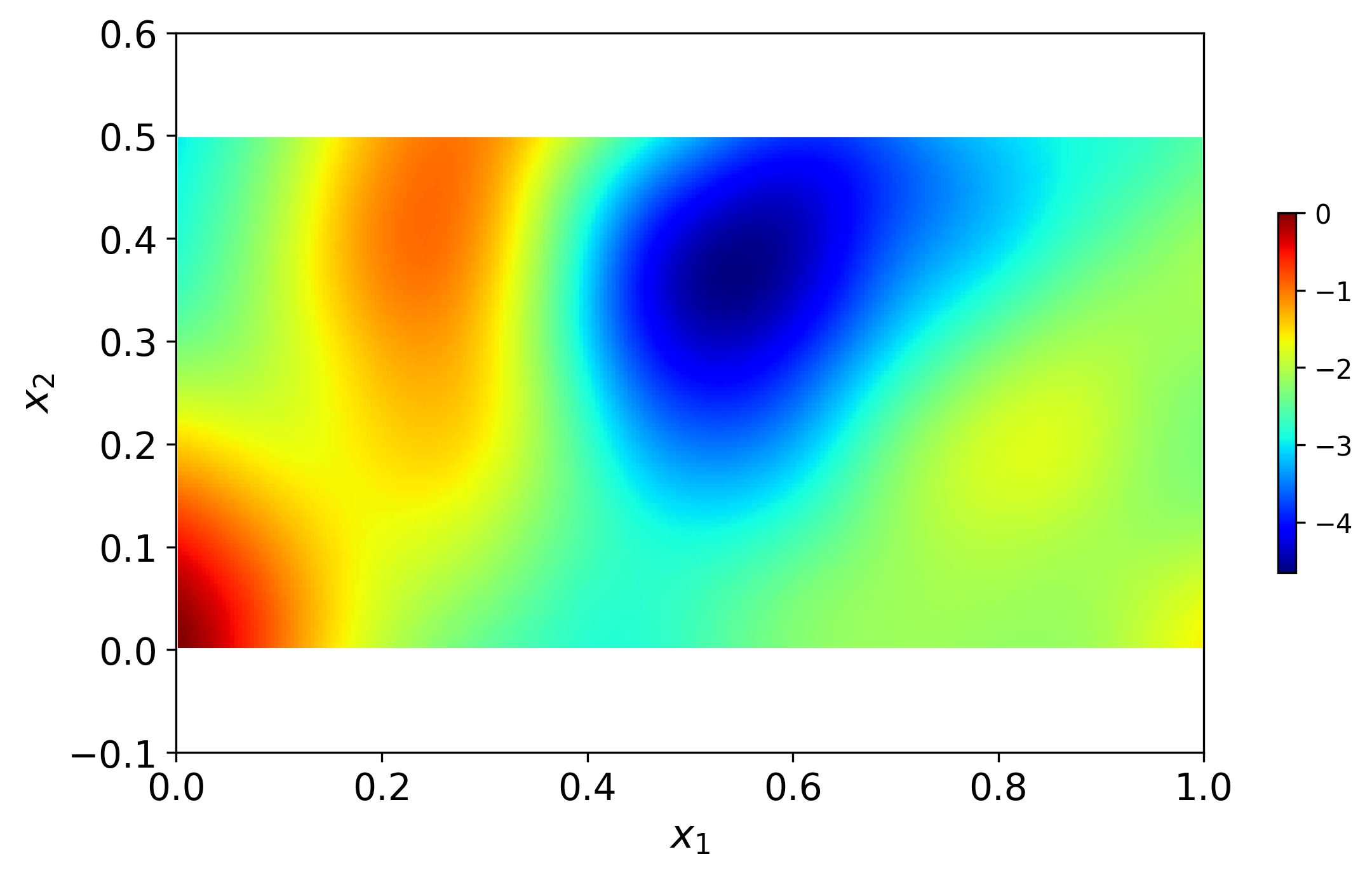
In the considered examples, we set x1βˆ—=0.15superscriptsubscriptπ‘₯10.15x_{1}^{*}=0.15, x2βˆ—=0.25superscriptsubscriptπ‘₯20.25x_{2}^{*}=0.25, M=1𝑀1M=1, Ξ΅=0.025πœ€0.025\varepsilon=0.025, Ο•=0.317italic-Ο•0.317\phi=0.317, H=0𝐻0H=0, q=1π‘ž1q=1, Ξ»=0.5πœ†0.5\lambda=0.5, and ΟƒY=0.9subscriptπœŽπ‘Œ0.9\sigma_{Y}=0.9. The conductivity field and initial condition for ADE are shown in Figure 3.
Refer to caption
(a)
Refer to caption
(b)
Figure 3: (a) The reference field Y​(𝐱)=ln⁑K​(𝐱)π‘Œπ±πΎπ±Y(\mathbf{x})=\ln K(\mathbf{x}) with the correlation length Ξ»=0.5πœ†0.5\lambda=0.5. (b) The initial condition for the solute transport problem in Eq (8).

To validate the PINN method, we solve the Darcy flow equation and forward ADE by the finite difference (FD) simulators MODFLOW [7] and MT3DMS [27], respectively. The latter simulator uses the implicit Total Variation Diminishing (TVD) solver for ADE. The FD solution for h​(𝐱)β„Žπ±h(\mathbf{x}) is obtained on a uniform 256Γ—128256128256\times 128 spatial grid and for u​(𝐱,t)𝑒𝐱𝑑u(\mathbf{x},t) on the same grid with adaptive time stepping and is saved on a uniform 100Γ—256Γ—128100256128100\times 256\times 128 time-space grid.

2.2 DNN representations in the PINN method

Here, our objective is to solve Eq (8) with the PINN method. This equation contains the velocity 𝐯​(𝐱)𝐯𝐱\mathbf{v}(\mathbf{x}), which is given by Eq (12). In the forward and backward ADE problems, we assume that K​(𝐱)𝐾𝐱K(\mathbf{x}) and h​(𝐱)β„Žπ±h(\mathbf{x}) in Eq (12) are known. In the inverse ADE problem, we compute 𝐯​(𝐱)𝐯𝐱\mathbf{v}(\mathbf{x}) (and estimate K​(𝐱)𝐾𝐱K(\mathbf{x}) and h​(𝐱)β„Žπ±h(\mathbf{x})) by solving a coupled inverse problem consisting of the ADE (8) and the flow equations (12) and (13).

2.2.1 DNN approximations of parameter fields and state variables

To take advantage of automatic differentiation (AD) [2], we approximate the state variables u​(𝐱,t)𝑒𝐱𝑑u(\mathbf{x},t) and h​(𝐱)β„Žπ±h(\mathbf{x}) and the space-dependent coefficient K​(𝐱)𝐾𝐱K(\mathbf{x}) with the three separate DNNs:

K​(𝐱)β‰ˆk^​(𝐱;Ξ±),h​(𝐱)β‰ˆh^​(𝐱;Ξ²),u​(𝐱,t)β‰ˆu^​(𝐱,t;Ξ³),formulae-sequence𝐾𝐱^π‘˜π±π›Όformulae-sequenceβ„Žπ±^β„Žπ±π›½π‘’π±π‘‘^𝑒𝐱𝑑𝛾\begin{split}K(\mathbf{x})\approx\hat{k}(\mathbf{x};\alpha),\\ h(\mathbf{x})\approx\hat{h}(\mathbf{x};\beta),\\ u(\mathbf{x},t)\approx\hat{u}(\mathbf{x},t;\gamma),\end{split} (14)

where α𝛼\alpha, β𝛽\beta, and γ𝛾\gamma are parameters (weights and biases) of the k^^π‘˜\hat{k}, h^^β„Ž\hat{h}, and u^^𝑒\hat{u} DNNs, respectively. Here, we use fully connected feed-forward DNNs, which have the form

𝒩​𝒩​(𝐳;ΞΈ):=ΟƒNh+1​(ΟƒNh​(ΟƒNhβˆ’1​(…​(Οƒ1​(𝐳))))),assignπ’©π’©π³πœƒsubscript𝜎subscriptπ‘β„Ž1subscript𝜎subscriptπ‘β„Žsubscript𝜎subscriptπ‘β„Ž1…subscript𝜎1𝐳\mathcal{NN}(\mathbf{z};\theta):=\sigma_{N_{h}+1}(\sigma_{N_{h}}(\sigma_{N_{h}-1}(...(\sigma_{1}(\mathbf{z}))))), (15)

where 𝐳𝐳\mathbf{z} is the input of the neural network (for k^^π‘˜\hat{k} and h^^β„Ž\hat{h}, 𝐳=𝐱𝐳𝐱\mathbf{z}=\mathbf{x}; for u^^𝑒\hat{u}, 𝐳=(𝐱,t)𝐳𝐱𝑑\mathbf{z}=(\mathbf{x},t)), ΞΈπœƒ\theta is the assembly of DNN parameters, Nhsubscriptπ‘β„ŽN_{h} is the number of the hidden layers, and

Οƒi​(𝐳i)=ΟƒβŠ™(𝐖i​𝐳i+𝐛i)subscriptπœŽπ‘–subscript𝐳𝑖direct-product𝜎subscript𝐖𝑖subscript𝐳𝑖subscript𝐛𝑖\sigma_{i}(\mathbf{z}_{i})=\sigma\odot(\mathbf{W}_{i}\mathbf{z}_{i}+\mathbf{b}_{i}) (16)

where ΟƒπœŽ\sigma is the activation function, βŠ™direct-product\odot represents the element-wise operation, 𝐳i=Οƒiβˆ’1​(𝐳iβˆ’1)subscript𝐳𝑖subscriptπœŽπ‘–1subscript𝐳𝑖1\mathbf{z}_{i}=\sigma_{i-1}(\mathbf{z}_{i-1}), and 𝐳1=𝐳subscript𝐳1𝐳\mathbf{z}_{1}=\mathbf{z}. Here, we use the hyperbolic tangent activation function Οƒi​(β‹…)=tanh⁑(β‹…)subscriptπœŽπ‘–β‹…β‹…\sigma_{i}(\cdot)=\tanh(\cdot) for i∈{1,…,Nh}𝑖1…subscriptπ‘β„Ži\in\{1,...,N_{h}\}, which satisfies the requirement of being at least twice continuously differentiable in 𝐱𝐱\mathbf{x}, which is needed for solving the second-order PDE. The choice of the activation function in the output layer (i=Nh+1𝑖subscriptπ‘β„Ž1i=N_{h}+1) is problem specific. For the forward and inverse ADEs, we use the identity activation function:

ΟƒNh+1​(𝐳Nh+1)=𝐖Nh+1​𝐳Nh+1+𝐛Nh+1.subscript𝜎subscriptπ‘β„Ž1subscript𝐳subscriptπ‘β„Ž1subscript𝐖subscriptπ‘β„Ž1subscript𝐳subscriptπ‘β„Ž1subscript𝐛subscriptπ‘β„Ž1\sigma_{N_{h}+1}(\mathbf{z}_{N_{h}+1})=\mathbf{W}_{N_{h}+1}\mathbf{z}_{N_{h}+1}+\mathbf{b}_{N_{h}+1}. (17)

For the backward ADE, we employ a nonlinear positive (sigmoid) activation function to strictly enforce the positivity of the solution. For i∈{1,…,Nh+1}𝑖1…subscriptπ‘β„Ž1i\in\{1,...,N_{h+1}\}, 𝐖iβˆˆβ„Nni+1Γ—Nnisubscript𝐖𝑖superscriptℝsuperscriptsubscript𝑁𝑛𝑖1superscriptsubscript𝑁𝑛𝑖\mathbf{W}_{i}\in\mathbb{R}^{N_{n}^{i+1}\times{N_{n}^{i}}} is the weight matrix connecting two adjacent layers and 𝐛iβˆˆβ„Nni+1subscript𝐛𝑖superscriptℝsuperscriptsubscript𝑁𝑛𝑖1\mathbf{b}_{i}\in\mathbb{R}^{N_{n}^{i+1}} is the bias vector, where Nnisuperscriptsubscript𝑁𝑛𝑖N_{n}^{i} is the number of neurons for layer i𝑖i. There are other at least twice differential activation functions, including the sigmoid function, which varies from 0 to 1. We choose the tanh activation because it has better convergence properties [15]. In all DNNs, we fix the number of hidden layers to Nh=5subscriptπ‘β„Ž5N_{h}=5. The number of neurons in each hidden layer Nnsubscript𝑁𝑛N_{n} is kept the same. The effect of Nnsubscript𝑁𝑛N_{n} on the PINN solution accuracy is reported in Section 4.

2.3 PINN formulation for forward and backward ADEs

In groundwater models, the functional form of K​(𝐱)𝐾𝐱K(\mathbf{x}) is usually not known–instead, it is given at a set of points, e.g., on the FD mesh. The mesh values Kn=K​(𝐱nK)subscript𝐾𝑛𝐾superscriptsubscript𝐱𝑛𝐾K_{n}=K(\mathbf{x}_{n}^{K}) of K𝐾K are found by solving an inverse problem or generated as a realization of a correlated random field with known statistics. Here, we train k^​(𝐱;Ξ±)^π‘˜π±π›Ό\hat{k}(\mathbf{x};\alpha) using a set of conductivity measurements {Kn}n=1Nksuperscriptsubscriptsubscript𝐾𝑛𝑛1subscriptπ‘π‘˜\{K_{n}\}_{n=1}^{N_{k}}, which are randomly sampled from the K𝐾K mesh values, by minimizing the loss function Lk​(Ξ±)subscriptπΏπ‘˜π›ΌL_{k}(\alpha),

Ξ±βˆ—=minα⁑{Lk^​(Ξ±)=1Nkβ€‹βˆ‘n=1Nk[k^​(𝐱n;Ξ±)βˆ’Kn]2}.superscript𝛼subscript𝛼subscript𝐿^π‘˜π›Ό1subscriptπ‘π‘˜superscriptsubscript𝑛1subscriptπ‘π‘˜superscriptdelimited-[]^π‘˜subscript𝐱𝑛𝛼subscript𝐾𝑛2\begin{split}\alpha^{*}=\min_{\alpha}\left\{L_{\hat{k}}(\alpha)=\frac{1}{N_{k}}\sum_{n=1}^{N_{k}}[\hat{k}({\mathbf{x}}_{n};\alpha)-{K}_{n}]^{2}\right\}.\end{split} (18)

For the forward and backward ADEs, we assume that h​(𝐱)β„Žπ±h(\mathbf{x}) is also known on the same mesh where K​(x)𝐾π‘₯K(x) is specified, and we train h^​(𝐱;Ξ²)^β„Žπ±π›½\hat{h}(\mathbf{x};\beta) by minimizing the loss function Lh​(Ξ²)subscriptπΏβ„Žπ›½L_{h}(\beta)

Ξ²βˆ—=minβ⁑{Lh^​(Ξ²)=1Nhβ€‹βˆ‘n=1Nh[h^​(𝐱n;Ξ²)βˆ’hn]2},superscript𝛽subscript𝛽subscript𝐿^β„Žπ›½1subscriptπ‘β„Žsuperscriptsubscript𝑛1subscriptπ‘β„Žsuperscriptdelimited-[]^β„Žsubscript𝐱𝑛𝛽subscriptβ„Žπ‘›2\displaystyle\beta^{*}=\min_{\beta}\left\{L_{\hat{h}}(\beta)=\frac{1}{N_{h}}\sum_{n=1}^{N_{h}}[\hat{h}({\mathbf{x}}_{n};\beta)-h_{n}]^{2}\right\}, (19)

where {hn}n=1Nhsuperscriptsubscriptsubscriptβ„Žπ‘›π‘›1subscriptπ‘β„Ž\{h_{n}\}_{n=1}^{N_{h}} are sampled from the head values on the finite difference mesh. For the considered problem and DNN size, we find that the DNN approximation errors for both K𝐾K and hβ„Žh are less than 0.5%percent0.50.5\%, which is much smaller than the errors in the PINN solutions of ADEs presented below. Therefore, we disregard the DNN approximations of the known K𝐾K and hβ„Žh fields as potential sources of errors in the PINN solutions.

The k^^π‘˜\hat{k} and h^^β„Ž\hat{h} DNNs are used to compute a DNN approximation of 𝐯​(x)𝐯π‘₯\mathbf{v}(x) based on the Darcy equation (12):

𝐯^​(𝐱;Ξ±,Ξ²)=βˆ’k^​(𝐱;Ξ±)Ο•β€‹βˆ‡h^​(𝐱;Ξ²),^𝐯𝐱𝛼𝛽^π‘˜π±π›Όitalic-Ο•βˆ‡^β„Žπ±π›½\hat{\mathbf{v}}(\mathbf{x};\alpha,\beta)=-\frac{\hat{k}(\mathbf{x};\alpha)}{\phi}\nabla\hat{h}(\mathbf{x};\beta), (20)

Here, α𝛼\alpha and β𝛽\beta are estimated in Eqs (18) and (19), and the gradients are evaluated using AD.

The PINN solution of the forward or backward ADE (8) is formulated as

Ξ³βˆ—=minΞ³{Lu^(Ξ³)\displaystyle\gamma^{*}=\min_{\gamma}\Big{\{}L_{\hat{u}}(\gamma) =\displaystyle= Ξ»i​cNi​cβˆ‘n=1Ni​c[u^(𝐱n,t=0;Ξ³)βˆ’u(𝐱n,t=0)]2\displaystyle\frac{\lambda_{ic}}{N_{ic}}\sum_{n=1}^{N_{ic}}\left[\hat{u}({\mathbf{x}}_{n},t=0;\gamma)-u({\mathbf{x}}_{n},t=0)\right]^{2}
+\displaystyle+ Ξ»b​c​nNb​c​nxΓ—Nb​c​ntβ€‹βˆ‘n=1Nb​c​nxβˆ‘m=1Nb​c​nt[ℬu​(𝐱n,tm;Ξ³)]2subscriptπœ†π‘π‘π‘›superscriptsubscript𝑁𝑏𝑐𝑛π‘₯superscriptsubscript𝑁𝑏𝑐𝑛𝑑superscriptsubscript𝑛1superscriptsubscript𝑁𝑏𝑐𝑛π‘₯superscriptsubscriptπ‘š1superscriptsubscript𝑁𝑏𝑐𝑛𝑑superscriptdelimited-[]subscriptℬ𝑒subscript𝐱𝑛subscriptπ‘‘π‘šπ›Ύ2\displaystyle\frac{\lambda_{bcn}}{N_{bcn}^{x}\times N_{bcn}^{t}}\sum_{n=1}^{N_{bcn}^{x}}\sum_{m=1}^{N_{bcn}^{t}}\left[\mathcal{B}_{u}(\mathbf{x}_{n},t_{m};\gamma)\right]^{2}
+\displaystyle+ Ξ»b​c​dNb​c​dxΓ—Nb​c​dtβ€‹βˆ‘n=1Nb​c​dxβˆ‘m=1Nb​c​dt[u^​(𝐱n,tn;Ξ³)βˆ’gd​(𝐱n)]2subscriptπœ†π‘π‘π‘‘superscriptsubscript𝑁𝑏𝑐𝑑π‘₯superscriptsubscript𝑁𝑏𝑐𝑑𝑑superscriptsubscript𝑛1superscriptsubscript𝑁𝑏𝑐𝑑π‘₯superscriptsubscriptπ‘š1superscriptsubscript𝑁𝑏𝑐𝑑𝑑superscriptdelimited-[]^𝑒subscript𝐱𝑛subscript𝑑𝑛𝛾subscript𝑔𝑑subscript𝐱𝑛2\displaystyle\frac{\lambda_{bcd}}{N_{bcd}^{x}\times N_{bcd}^{t}}\sum_{n=1}^{N_{bcd}^{x}}\sum_{m=1}^{N_{bcd}^{t}}[\hat{u}(\mathbf{x}_{n},t_{n};\gamma)-g_{d}(\mathbf{x}_{n})]^{2}
+\displaystyle+ Ξ»r​e​sNr​e​sβˆ‘n=1Nr​e​s[β„›u^(𝐱n,tn;Ξ³)]2}\displaystyle\frac{\lambda_{res}}{N_{res}}\sum_{n=1}^{N_{res}}[\mathcal{R}_{\hat{u}}(\mathbf{x}_{n},t_{n};\gamma)]^{2}\Big{\}}

where β„›u^(𝐱,t;Ξ³)=u^t(𝐱,t;Ξ³)+βˆ‡β‹…[𝐯^(𝐱)u^(𝐱,t;Ξ³)]βˆ’βˆ‡β‹…[πƒβˆ‡u^((𝐱,t;Ξ³)]\mathcal{R}_{\hat{u}}(\mathbf{x},t;\gamma)=\hat{u}_{t}(\mathbf{x},t;\gamma)+\nabla\cdot[\hat{\mathbf{v}}(\mathbf{x})\hat{u}(\mathbf{x},t;\gamma)]-\nabla\cdot[\mathbf{D}\nabla\hat{u}(\mathbf{(}\mathbf{x},t;\gamma)] is the residual term, ℬu(𝐱n,tm;Ξ³)=βˆ‡u^(𝐱,tm;Ξ³)|𝐱=𝐱nβ‹…π§βˆ’gn(𝐱n)\mathcal{B}_{u}(\mathbf{x}_{n},t_{m};\gamma)=\nabla\hat{u}(\mathbf{x},t_{m};\gamma)\Big{\rvert}_{\mathbf{x}=\mathbf{x}_{n}}\cdot\mathbf{n}-g_{n}(\mathbf{x}_{n}) is the Neumann boundary operator, and 𝐧𝐧\mathbf{n} is the unit vector normal to boundaries where 𝐱nsubscript𝐱𝑛\mathbf{x}_{n} is sampled. The coefficients Ξ»i​csubscriptπœ†π‘–π‘\lambda_{ic}, Ξ»b​c​nsubscriptπœ†π‘π‘π‘›\lambda_{bcn}, Ξ»b​c​dsubscriptπœ†π‘π‘π‘‘\lambda_{bcd}, and Ξ»r​e​ssubscriptπœ†π‘Ÿπ‘’π‘ \lambda_{res} are the weights corresponding to the initial, Neumann boundary, and Dirichlet boundary conditions, and the ADE residual, respectively. We randomly sample the initial concentration values at Ni​csubscript𝑁𝑖𝑐{N_{ic}} spacial locations, where Ni​csubscript𝑁𝑖𝑐N_{ic} equals 75%percent7575\% of the initial nodal values on the finite volume mesh (i.e., Ni​c=0.75Γ—256Γ—128=26,274formulae-sequencesubscript𝑁𝑖𝑐0.7525612826274N_{ic}=0.75\times 256\times 128=26,274). We enforce the boundary conditions at Nb​c​nt=Nb​c​dt=Nt=100subscriptsuperscript𝑁𝑑𝑏𝑐𝑛subscriptsuperscript𝑁𝑑𝑏𝑐𝑑subscript𝑁𝑑100N^{t}_{bcn}=N^{t}_{bcd}=N_{t}=100 equal time intervals. At each time interval, we use the LHS scheme to sample 54 points on boundaries in the x2subscriptπ‘₯2x_{2} direction and 128 points on the boundaries in the x1subscriptπ‘₯1x_{1} direction. As result, the Dirichlet BC is enforced at Nb​c​dx=54superscriptsubscript𝑁𝑏𝑐𝑑π‘₯54N_{bcd}^{x}=54 spatial locations and the Neumann BCs are enforced at Nb​c​nx=128Γ—2+54superscriptsubscript𝑁𝑏𝑐𝑛π‘₯128254N_{bcn}^{x}=128\times 2+54 spatial locations. The ADE residual is enforced at Nr​e​ssubscriptπ‘π‘Ÿπ‘’π‘ N_{res} points in the space-time domain. In the following sections, we study the accuracy of PINN solutions as functions of the number and distributions of the residual points. Algorithm 1 below encapsulates the complete training process.

The DNN approximations of u𝑒u and 𝐯𝐯\mathbf{v} make the PINN ADE model β€œanalytically differentiable,” and all partial derivatives in the ADE (8) can be computed using AD, which is important for estimating the ADE residuals without numerically discretizing the derivatives. Also, in the PINN ADE model, the gradients with respect to the parameter vectors α𝛼\alpha and β𝛽\beta can be computed with AD, which is needed for the back-propagation step in the DNN training.

Step 1: Initialize parameters α𝛼\alpha, β𝛽\beta, and γ𝛾\gamma of three neural networks using the Xavier initialization scheme.
Step 2: Train k^​(𝐱;Ξ±)^π‘˜π±π›Ό\hat{k}(\mathbf{x};\alpha) by minimizing the loss function (18) so that Ξ±βˆ—=a​r​g​m​i​n​Lk​(Ξ±)superscriptπ›Όπ‘Žπ‘Ÿπ‘”π‘šπ‘–π‘›subscriptπΏπ‘˜π›Ό{\alpha}^{*}=argminL_{k}(\alpha)
Step 3: Train h^​(𝐱;Ξ²)^β„Žπ±π›½\hat{h}(\mathbf{x};\beta) by minimizing the loss function (19) so that Ξ²βˆ—=a​r​g​m​i​n​Lh​(Ξ²)superscriptπ›½π‘Žπ‘Ÿπ‘”π‘šπ‘–π‘›subscriptπΏβ„Žπ›½{\beta}^{*}=argminL_{h}(\beta)
Step 4: Find solution in the form u^​(𝐱,t;Ξ³)^𝑒𝐱𝑑𝛾\hat{u}(\mathbf{x},t;\gamma) by minimizing the loss function (2.3): Ξ³βˆ—=a​r​g​m​i​n​Lu​(Ξ³)superscriptπ›Ύπ‘Žπ‘Ÿπ‘”π‘šπ‘–π‘›subscript𝐿𝑒𝛾{\gamma}^{*}=argminL_{u}(\gamma)

Algorithm 1 PINN algorithm for solving forward and backward ADEs (8)

2.4 Neural network training

Following [8], we use a ”two-step” approach to minimize the loss function in Eqs (18), (19), and (2.3), where the Adam optimizer [13] is employed at the first step and the L-BFGS-B (quasi-Newton) optimizer [16] is used at the second step. For training k^​(𝐱;Ξ±)^π‘˜π±π›Ό\hat{k}(\mathbf{x};\alpha) and h^​(𝐱;Ξ²)^β„Žπ±π›½\hat{h}(\mathbf{x};\beta), the Adam optimizer is run for 30,0003000030,000 epochs with a fixed learning rate of 0.0010.0010.001. In training u^​(𝐱,t;Ξ³)^𝑒𝐱𝑑𝛾\hat{u}(\mathbf{x},t;\gamma), the Adam optimizer is run for 200,000200000200,000 epochs with a fixed learning rate of 0.00020.00020.0002. The mini-batch size is set to 1,00010001,000. The L-BFGS-B algorithm is terminated either when the magnitude of the loss function is less than a prescribed tolerance of 10βˆ’7superscript10710^{-7} or the number of iterations (training epochs) exceeds 50,0005000050,000. The DNNs weights and biases are randomly initialized using the Xavier initialization [5].

All simulations in this work are performed on a PC with NVIDIA GeForce RTX 2070 Max-Q GPU. We find that the training time increases with the DNN size and the number of residual points. In the considered examples, the training time ranges from approximately 8 core hours to 12 core hours.

2.5 Limitations of PINN for the ADE with Gaussian source initial conditions

PINN was shown to be accurate for solving ADEs with certain initial and boundary conditions. For example, in [9], PINN was used to solve the two-dimensional time-dependent ADE in a non-uniform flow field with the zero initial condition, u=f​(x)𝑒𝑓π‘₯u=f(x) was prescribed at the upstream boundary, and the homogeneous Neumann BC was assigned at the downstream boundary. The maximum and minimum of f​(x)𝑓π‘₯f(x) are 1 and 0, correspondingly. For these BCs, the maximum and minimum of u​(𝐱,t)𝑒𝐱𝑑u(\mathbf{x},t) are 1 and 0, respectively, at all times. An accurate PINN solution for this problem was obtained with the empirically determined weights Ξ»i​c=Ξ»b​c​n=Ξ»b​c​d=10subscriptπœ†π‘–π‘subscriptπœ†π‘π‘π‘›subscriptπœ†π‘π‘π‘‘10\lambda_{ic}=\lambda_{bcn}=\lambda_{bcd}=10 and Ξ»r​e​s=1subscriptπœ†π‘Ÿπ‘’π‘ 1\lambda_{res}=1.

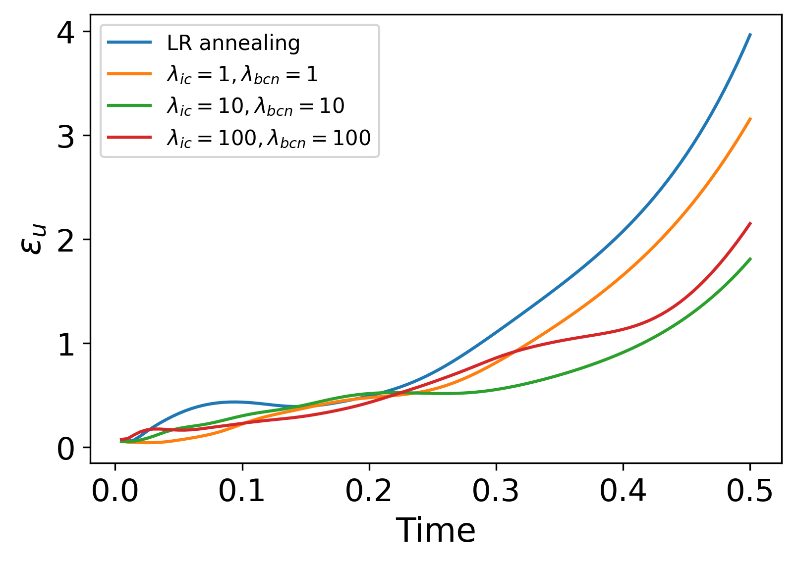
However, we find that applying the PINN method to the ADE (8) with a Gaussian source initial condition (9) does not produce an accurate solution. The relative L2 error in this solution is shown in Figure 4(a) for four different combinations of the weights in the loss function. Here and later in this work, we define the relative L2 error at time t𝑑t as

Ξ΅u​(t)=βˆ‘j=1Nt​o​t[u​(𝐱j,t)βˆ’u^​(𝐱j,t)]2βˆ‘j=1Nt​o​t[u​(𝐱j,t)]2subscriptπœ€π‘’π‘‘superscriptsubscript𝑗1subscriptπ‘π‘‘π‘œπ‘‘superscriptdelimited-[]𝑒subscript𝐱𝑗𝑑^𝑒subscript𝐱𝑗𝑑2superscriptsubscript𝑗1subscriptπ‘π‘‘π‘œπ‘‘superscriptdelimited-[]𝑒subscript𝐱𝑗𝑑2\varepsilon_{u}(t)=\sqrt{\frac{\sum_{j=1}^{N_{tot}}\left[u(\mathbf{x}_{j},t)-\hat{u}(\mathbf{x}_{j},t)\right]^{2}}{\sum_{j=1}^{N_{tot}}\left[u(\mathbf{x}_{j},t)\right]^{2}}} (22)

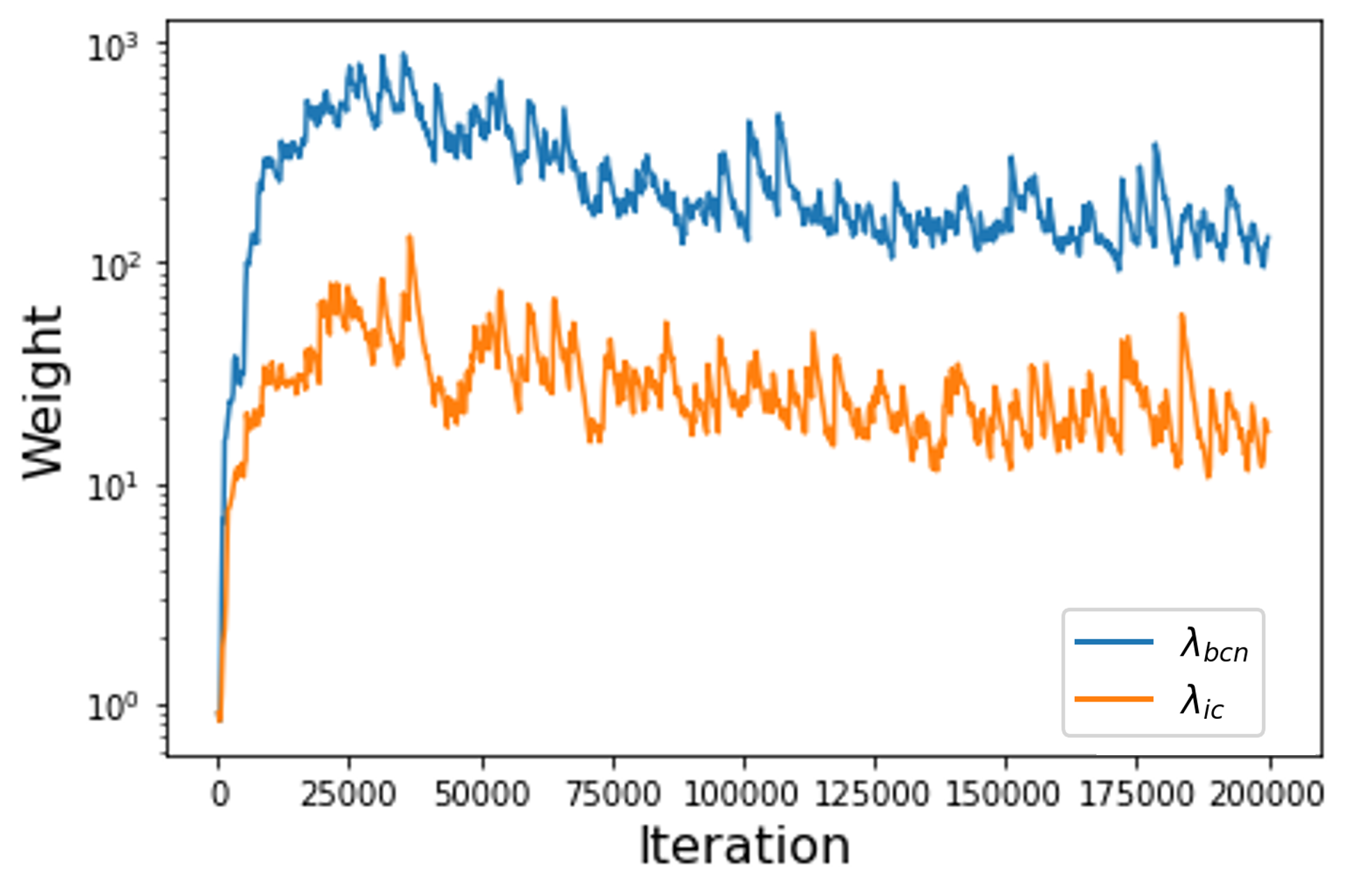
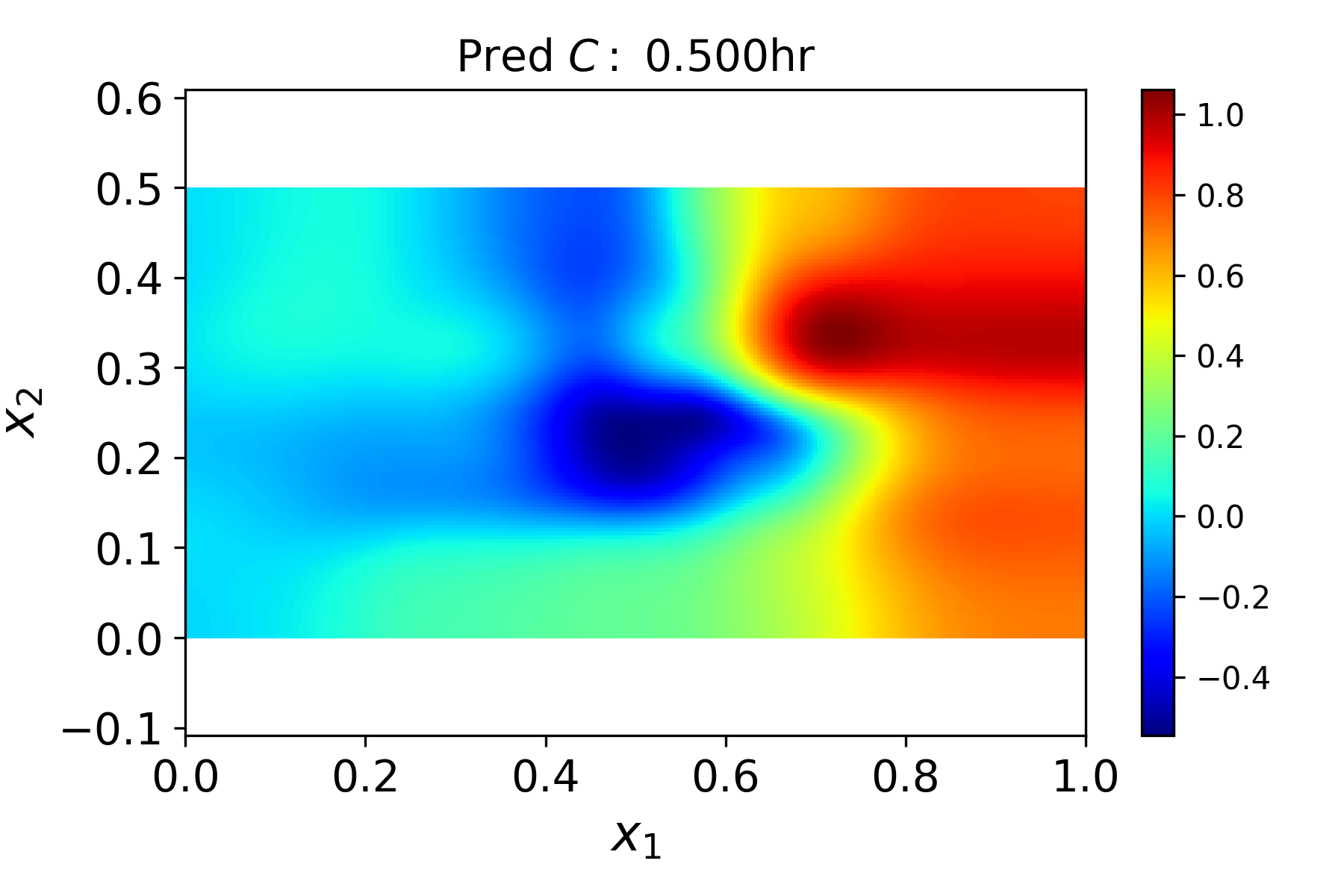
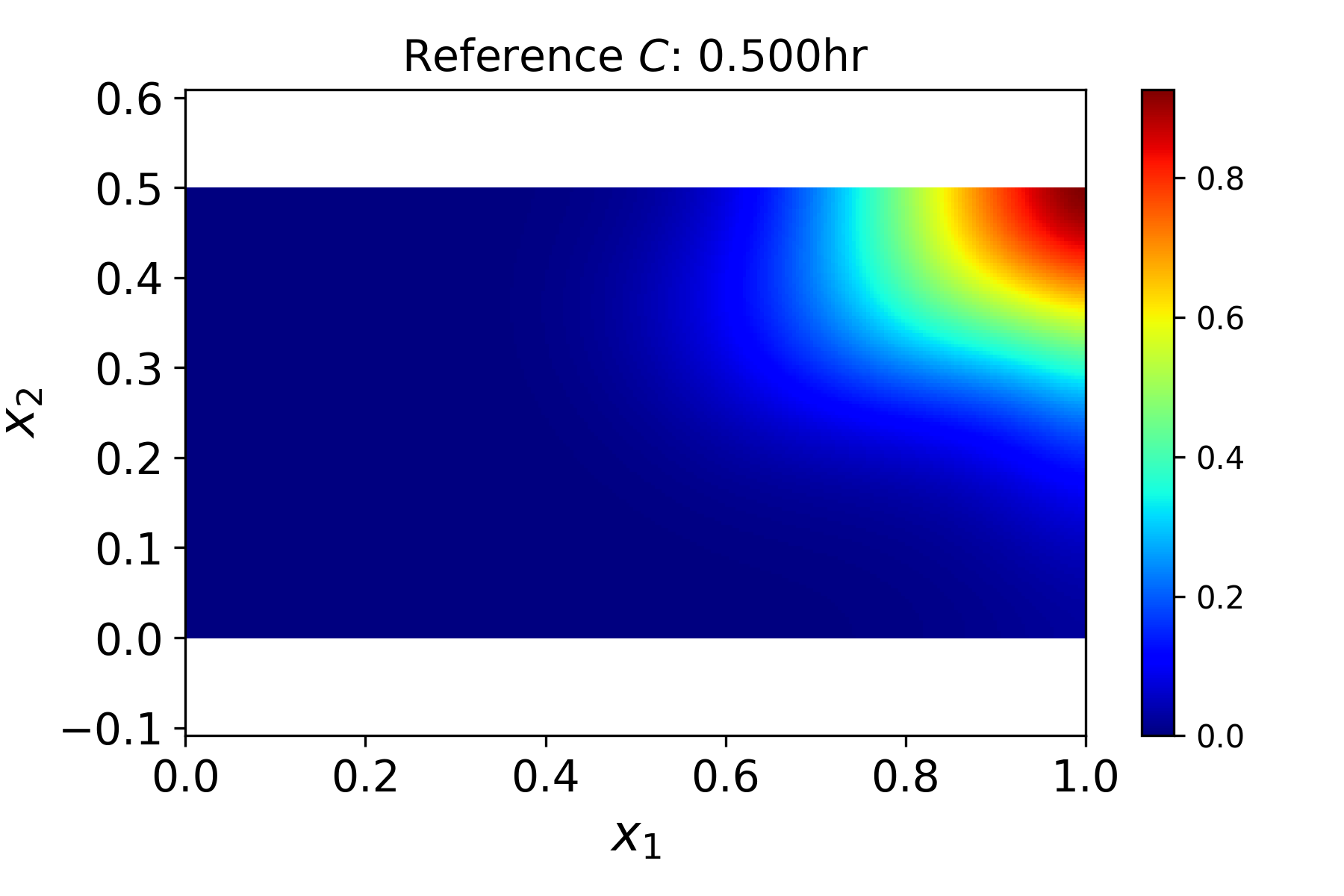
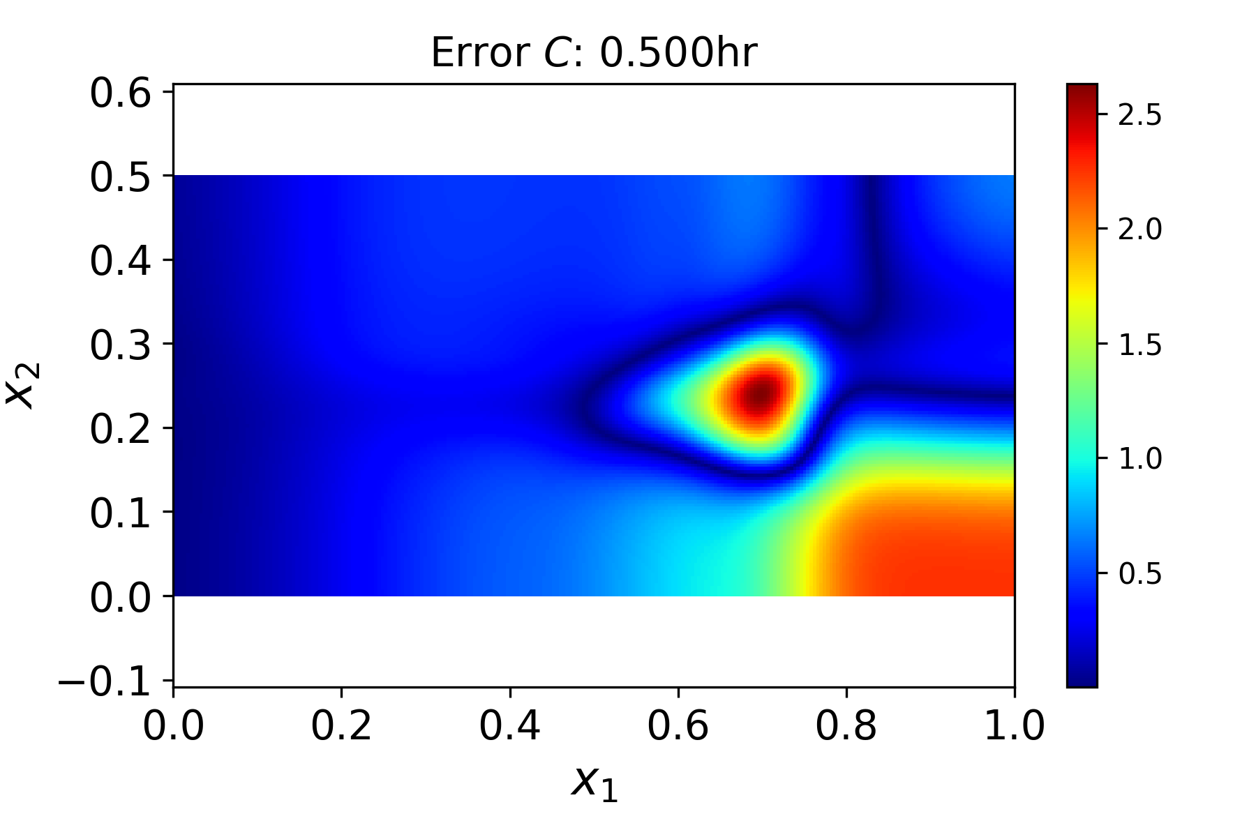
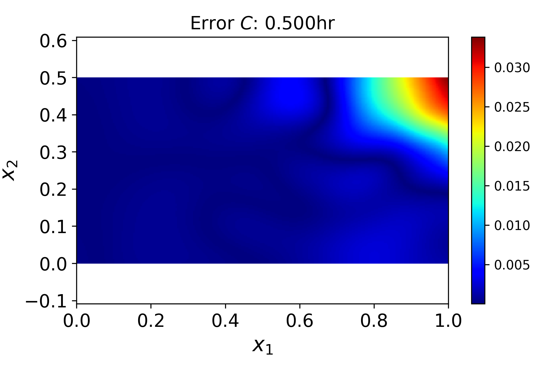
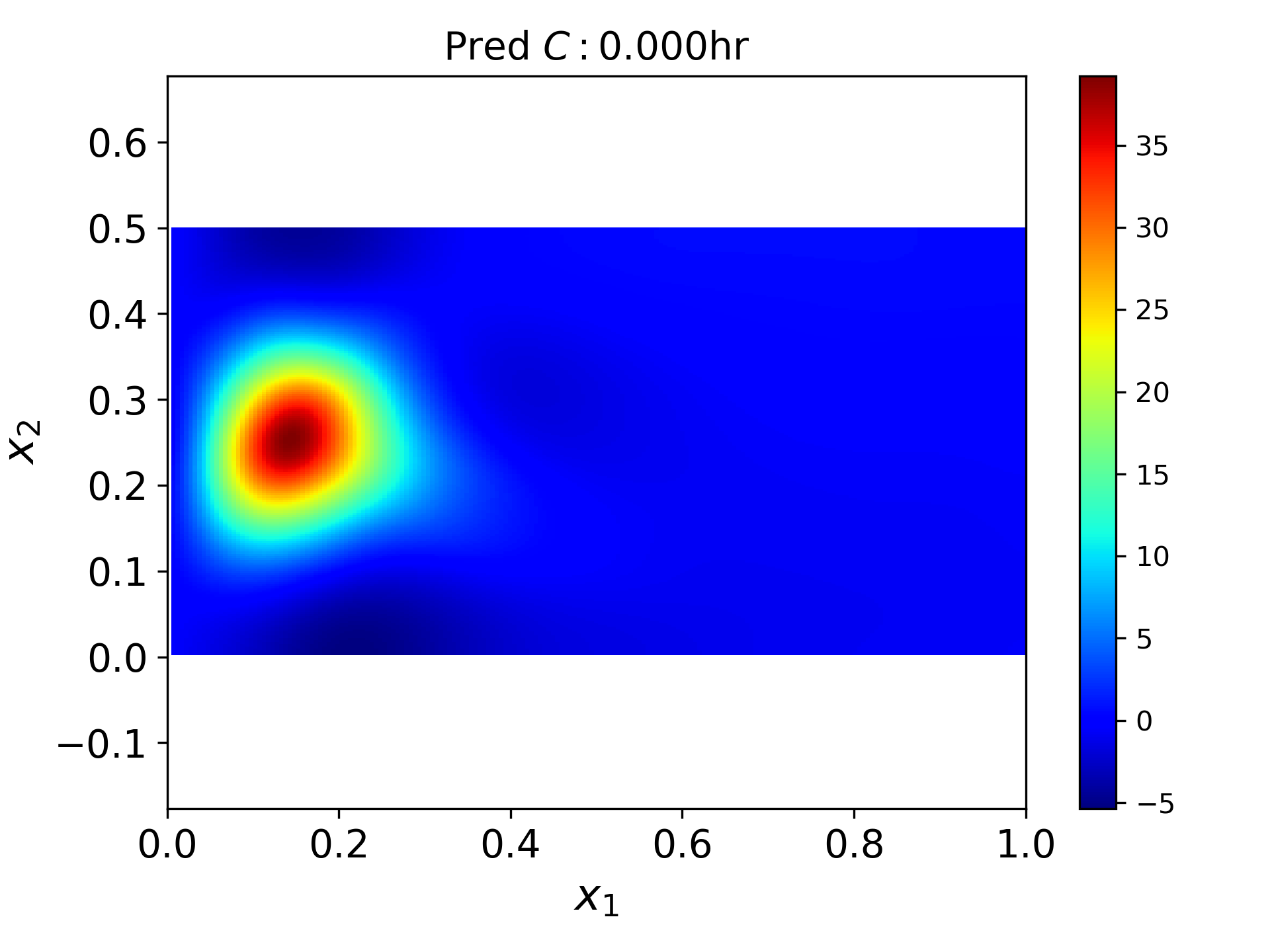
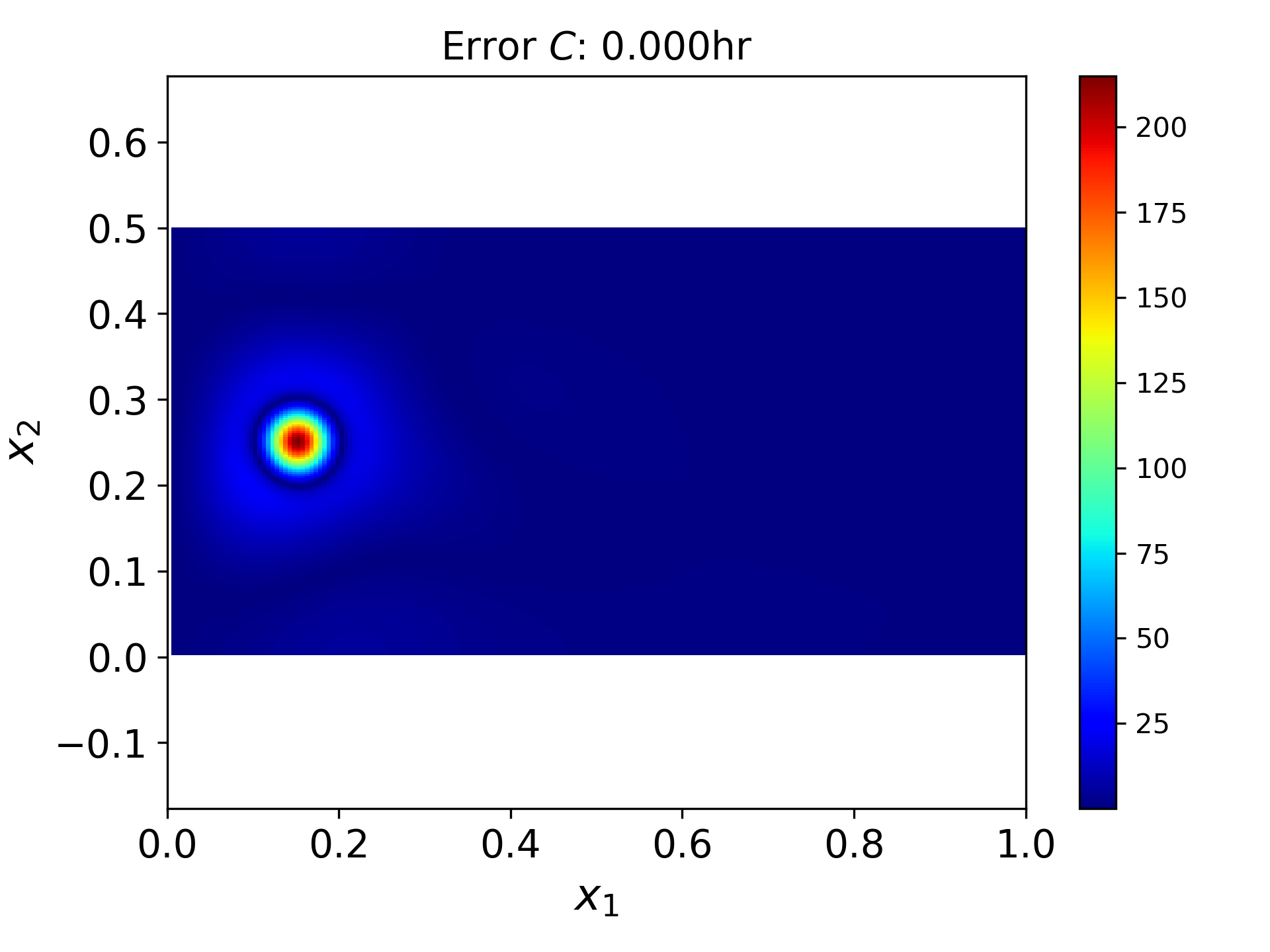
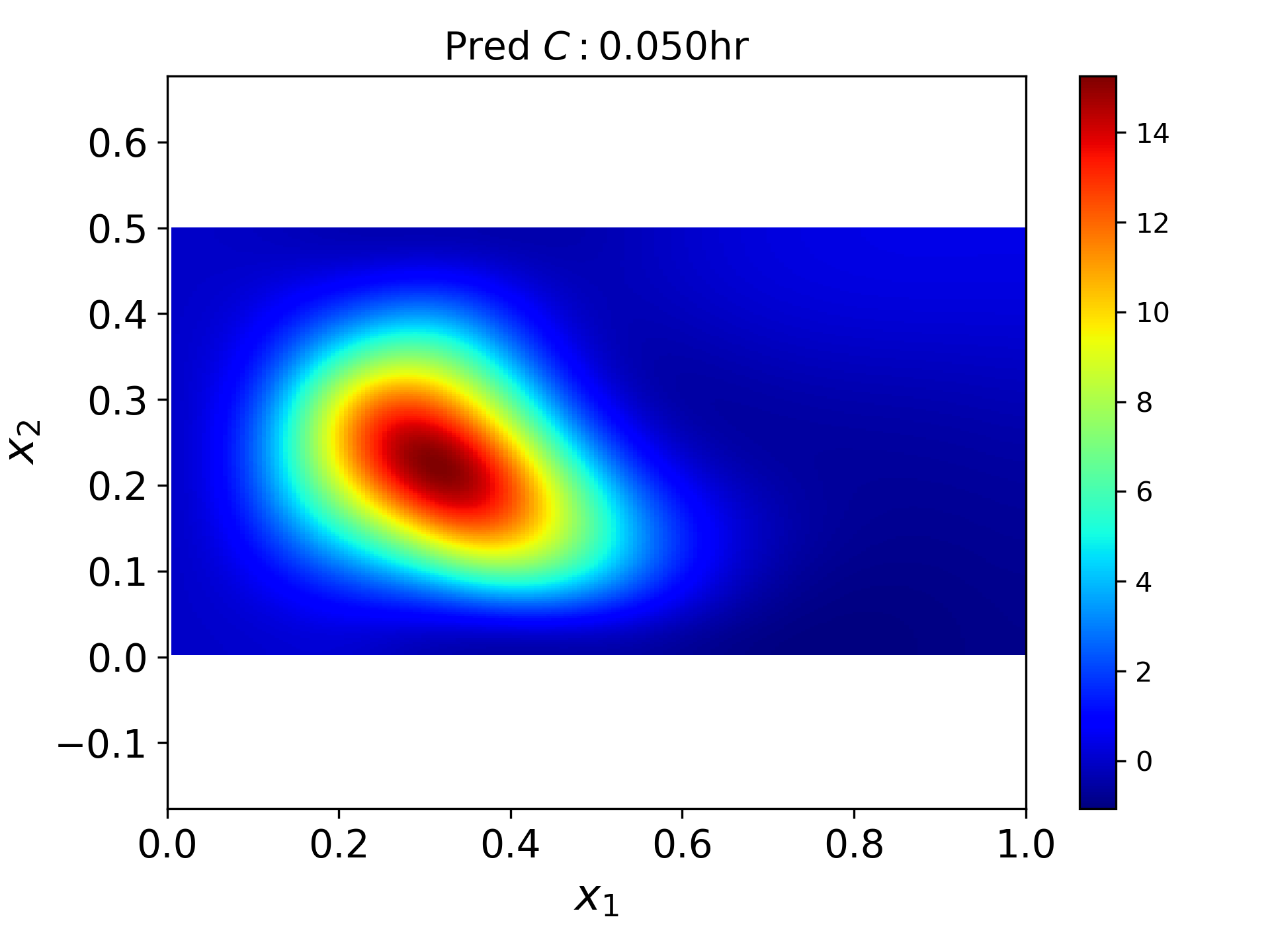
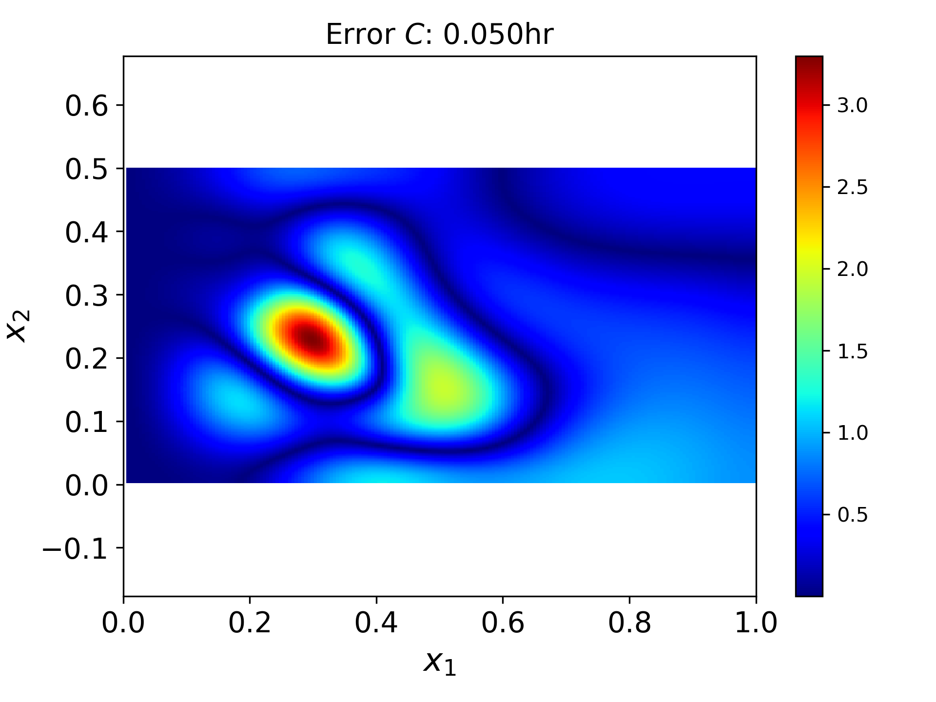
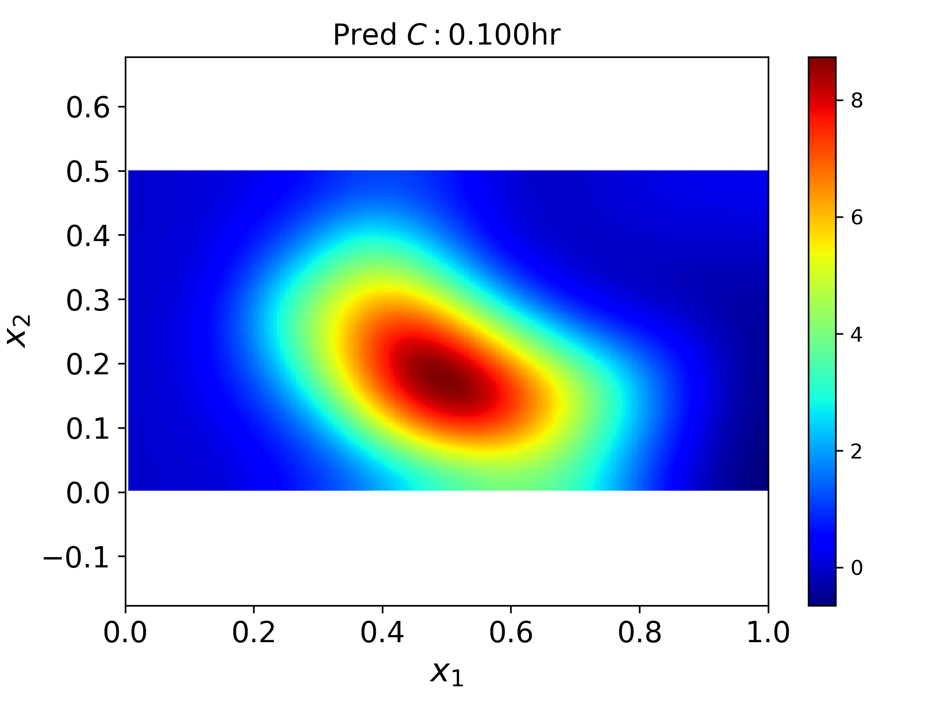
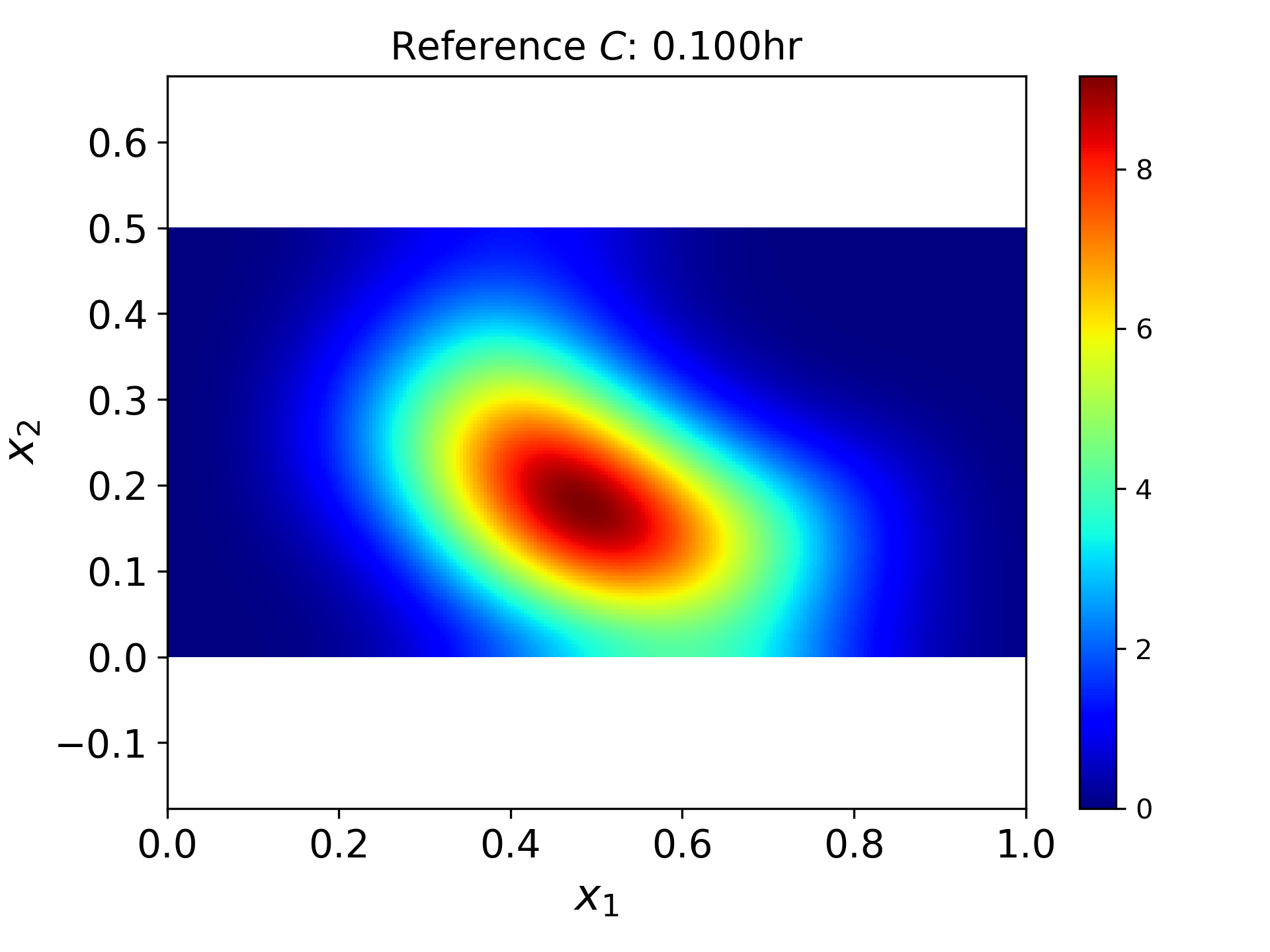
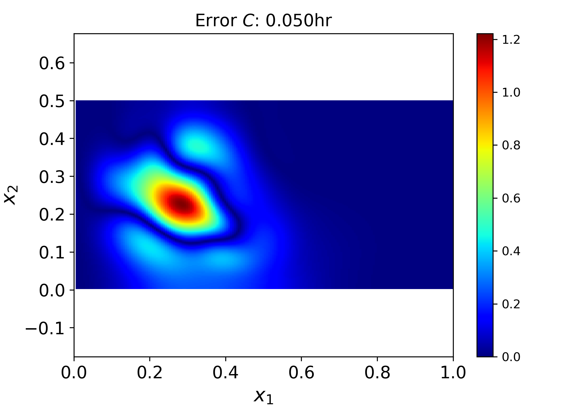
where Nt​o​tsubscriptπ‘π‘‘π‘œπ‘‘N_{tot} is the mesh size in the reference FD solution. For all considered weight choices, the L2 errors increase with time, with the maximum errors ranging from 180% to near 400%. These solutions are obtained on the time domain t∈(0,0.5]𝑑00.5t\in(0,0.5], with Nr​e​s=100,000subscriptπ‘π‘Ÿπ‘’π‘ 100000N_{res}=100,000 residual points randomly chosen using LHS across the time-space domain and the DNN width set to Nn=60subscript𝑁𝑛60N_{n}=60. The four combinations of weights are selected as follows. In all four cases, we set Ξ»r​e​s=1subscriptπœ†π‘Ÿπ‘’π‘ 1\lambda_{res}=1 and Ξ»i​c=Ξ»b​c​dsubscriptπœ†π‘–π‘subscriptπœ†π‘π‘π‘‘\lambda_{ic}=\lambda_{bcd}. In the first case, the remaining weights Ξ»i​csubscriptπœ†π‘–π‘\lambda_{ic} and Ξ»b​c​nsubscriptπœ†π‘π‘π‘›\lambda_{bcn} are computed according to the learning rate annealing algorithm [25]. This algorithm updates the weights during the training to balance the gradients of all terms in the loss function. The resulting values of Ξ»i​csubscriptπœ†π‘–π‘\lambda_{ic} and Ξ»b​c​nsubscriptπœ†π‘π‘π‘›\lambda_{bcn} are shown in Figure 4(b). In cases 2–4, we set the weights statically, i.e., the weights do not change during training. We use the weights Ξ»i​c=Ξ»b​c​d=Ξ»b​c​n=10subscriptπœ†π‘–π‘subscriptπœ†π‘π‘π‘‘subscriptπœ†π‘π‘π‘›10\lambda_{ic}=\lambda_{bcd}=\lambda_{bcn}=10 from [9] and two additional sets, Ξ»i​c=Ξ»b​c​d=Ξ»b​c​n=1subscriptπœ†π‘–π‘subscriptπœ†π‘π‘π‘‘subscriptπœ†π‘π‘π‘›1\lambda_{ic}=\lambda_{bcd}=\lambda_{bcn}=1 and 100100100. The smallest L2 error corresponds to the weights selected according to [9], and the largest errors are produced by the learning rate annealing algorithm. In Figure 11, we plot four snapshots of the PINN solution obtained with Ξ»i​c=Ξ»b​c​d=Ξ»b​c​n=10subscriptπœ†π‘–π‘subscriptπœ†π‘π‘π‘‘subscriptπœ†π‘π‘π‘›10\lambda_{ic}=\lambda_{bcd}=\lambda_{bcn}=10. Significant point errors are observed at all times, with the PINN solution becoming negative at time t=0.5𝑑0.5t=0.5.

Refer to caption
(a)
Refer to caption
(b)
Figure 4: (a) Relative L2subscript𝐿2L_{2} error in the PINN solutions of the forward ADE (8) subject to the initial condition (9) obtained with four different combinations of the weights in the loss function, including the weights selected according to the learning rate annealing method [25]. In all cases, Ξ»r​e​s=1subscriptπœ†π‘Ÿπ‘’π‘ 1\lambda_{res}=1 and Ξ»i​c=Ξ»b​dsubscriptπœ†π‘–π‘subscriptπœ†π‘π‘‘\lambda_{ic}=\lambda_{bd}. (b) Evolution of the weights Ξ»i​csubscriptπœ†π‘–π‘\lambda_{ic} and Ξ»b​nsubscriptπœ†π‘π‘›\lambda_{bn} (labeled as Ξ»b​csubscriptπœ†π‘π‘\lambda_{bc}) in the learning rate annealing algorithm.

The total error in a PINN solution can be decomposed in three parts: the optimization error, the estimation error, and the approximation error [21]. The approximation error comes from the finite-size of DNN and quantifies the distance between the class of functions that the given-size DNN can represent and the true PDE solution. The estimation error is due to approximating the integral loss function (1) with the discrete loss function (1). In general, this error should decrease with the increasing number of residual points. The optimization error is the error in solving the nonlinear least-square problem. This error strongly depends on the weight selection in the PINN loss function.

We attribute the high errors in the PINN solutions shown in Figure 4(a) to several factors. First, the maximum value of the solution um​a​x​(t)subscriptπ‘’π‘šπ‘Žπ‘₯𝑑u_{max}(t) exponentially decreases with time. This makes it difficult for a DNN with a finite size to approximate u​(𝐱,t)𝑒𝐱𝑑u(\mathbf{x},t) in the space-time domain, as demonstrated in Figure 1 for a solution of the one-dimensional ADE. Second, the LHS of the time-space domain with residual points in the PINN residual least-square formulation (1) might not be optimal for the ADE problem where the large time derivatives exist at early times. Finally, the selection of weights in the loss function in these solutions might not be optimal.

We find that increasing the number of residual points to 200,000 and the DNN width to 120 does not significantly decrease the L2 error. Theoretically, further increasing the DNN size and number of residual points should reduce the PINN error. However, such a brute-force approach could be computationally intractable for many real-world applications. In the next section, we propose several improvements that reduce the L2 error to less than 6% without increasing the DNN size and the number of residual points.

3 Improved PINN method

In this section, we propose a normalized ADE equation to reduce the approximation error in the PINN method. Next, we propose the adaptive sampling scheme for residual points to reduce the estimation error. Finally, we derive estimates of the weighting coefficients to reduce the minimization error.

3.1 Normalized PINN

A general rule for reducing the approximation and optimization errors in DNN models with the tanh and sigmoid activation functions is to normalize the DNN’s training dataset such that inputs are in the [-0.5,0.5] range (this normalization is related to the fact that derivatives of the activation function d​tanh⁑(z)/d​z𝑑𝑧𝑑𝑧d\tanh(z)/dz are very small for z𝑧z outside of the [-0.5,0.5] range) and the outputs are in the [0,1] range [12, 15]. Otherwise, the weights and biases of the DNN could be very large, which in turn might cause instabilities in the training process (large minimization errors). Usually, a dataset is normalized using a constant normalization factor. However, we demonstrated in Figure 1 that for u​(x,t)𝑒π‘₯𝑑u(x,t) with exponentially decreasing um​a​x​(t)=maxx⁑u​(x,t)subscriptπ‘’π‘šπ‘Žπ‘₯𝑑subscriptπ‘₯𝑒π‘₯𝑑u_{max}(t)=\max_{x}u(x,t), a more accurate training is achieved if the DNN is trained with the samples of u𝑒u normalized with the time-dependent factor um​a​x​(t)subscriptπ‘’π‘šπ‘Žπ‘₯𝑑u_{max}(t) rather than a constant factor, e.g., maxx,t⁑u​(x,t)subscriptπ‘₯𝑑𝑒π‘₯𝑑\max_{x,t}u(x,t). Below, we propose a similar normalization of the state variable u​(𝐱,t)𝑒𝐱𝑑u(\mathbf{x},t) in ADE (8).

We normalize the space and time coordinates in Eq (8) as t~=tTβˆ’0.5~𝑑𝑑𝑇0.5\tilde{t}=\frac{t}{T}-0.5, x~1=x1L1βˆ’0.5subscript~π‘₯1subscriptπ‘₯1subscript𝐿10.5\tilde{x}_{1}=\frac{x_{1}}{L_{1}}-0.5, and x~2=x2L2βˆ’0.5subscript~π‘₯2subscriptπ‘₯2subscript𝐿20.5\tilde{x}_{2}=\frac{x_{2}}{L_{2}}-0.5, where T𝑇T is the time horizon of the model. Next, we introduce a dimensionless variable u~​(𝐱,t)=u​(𝐱,t)g​(t)~𝑒𝐱𝑑𝑒𝐱𝑑𝑔𝑑\tilde{u}(\mathbf{x},t)=\frac{u(\mathbf{x},t)}{g(t)}, where g​(t)𝑔𝑑g(t) is the maximum of the solution u¯​(𝐱,t)¯𝑒𝐱𝑑\overline{u}(\mathbf{x},t) of the β€œmean-field” ADE

uΒ―t+𝐕​(𝐱)β‹…βˆ‡u¯​(𝐱)=βˆ‡β‹…[πƒβ€‹βˆ‡u¯​(𝐱)]subscriptΒ―π‘’π‘‘β‹…π•π±βˆ‡Β―π‘’π±β‹…βˆ‡delimited-[]πƒβˆ‡Β―π‘’π±\overline{u}_{t}+\mathbf{V}(\mathbf{x})\cdot\nabla\overline{u}(\mathbf{x})=\nabla\cdot[\mathbf{D}\nabla\overline{u}(\mathbf{x})]

defined on the two-dimensional infinite domain with the zero Dirichlet boundary conditions at plus/minus infinity and the initial condition (9). Here, 𝐕=[V,0]T𝐕superscript𝑉0𝑇\mathbf{V}=[V,0]^{T} is the mean-field velocity that solves the flow equation (13) with K​(𝐱)𝐾𝐱K(\mathbf{x}) replaced by its geometric average. The analytical solution of this equation is

u¯​(𝐱,t)=M2​π​Ρ2+2​Dx1​t​Ρ2+2​Dx2​t​exp⁑[βˆ’12​((x1βˆ’x1βˆ—βˆ’V​t)2Ξ΅2+2​Dx1​t+(x2βˆ’x2βˆ—)2Ξ΅2+2​Dx2​t)].¯𝑒𝐱𝑑𝑀2πœ‹superscriptπœ€22subscript𝐷subscriptπ‘₯1𝑑superscriptπœ€22subscript𝐷subscriptπ‘₯2𝑑12superscriptsubscriptπ‘₯1superscriptsubscriptπ‘₯1𝑉𝑑2superscriptπœ€22subscript𝐷subscriptπ‘₯1𝑑superscriptsubscriptπ‘₯2superscriptsubscriptπ‘₯22superscriptπœ€22subscript𝐷subscriptπ‘₯2𝑑\overline{u}(\mathbf{x},t)=\frac{M}{2\pi\sqrt{\varepsilon^{2}+2D_{x_{1}}t}\sqrt{\varepsilon^{2}+2D_{x_{2}}t}}\exp\left[-\frac{1}{2}(\frac{(x_{1}-x_{1}^{*}-Vt)^{2}}{\varepsilon^{2}+2D_{x_{1}}t}+\frac{(x_{2}-x_{2}^{*})^{2}}{\varepsilon^{2}+2D_{x_{2}}t})\right]. (23)

The maximum of u¯​(𝐱,t)¯𝑒𝐱𝑑\overline{u}(\mathbf{x},t) over 𝐱𝐱\mathbf{x} is

g​(t)=M2​π​Ρ2+2​Dx1​t​Ρ2+2​Dx2​t.𝑔𝑑𝑀2πœ‹superscriptπœ€22subscript𝐷subscriptπ‘₯1𝑑superscriptπœ€22subscript𝐷subscriptπ‘₯2𝑑g(t)=\frac{M}{2\pi\sqrt{\varepsilon^{2}+2D_{x_{1}}t}\sqrt{\varepsilon^{2}+2D_{x_{2}}t}}. (24)

The maximum of u​(𝐱,t)𝑒𝐱𝑑u(\mathbf{x},t) (the solution of Eq (8)) over 𝐱𝐱\mathbf{x} is well approximated by g​(t)𝑔𝑑g(t) as long as x1βˆ—+V​t<L1superscriptsubscriptπ‘₯1𝑉𝑑subscript𝐿1x_{1}^{*}+Vt<L_{1} (i.e., as long as the center of the plume stays within the domain). By introducing the additional dimensionless variables v~1=v1​TL1subscript~𝑣1subscript𝑣1𝑇subscript𝐿1\tilde{v}_{1}=v_{1}\frac{T}{L_{1}}, v~2=v2​TL2subscript~𝑣2subscript𝑣2𝑇subscript𝐿2\tilde{v}_{2}=v_{2}\frac{T}{L_{2}}, D~11=D11​TL12subscript~𝐷11subscript𝐷11𝑇superscriptsubscript𝐿12\tilde{D}_{11}=D_{11}\frac{T}{L_{1}^{2}} , D~22=D22​TL22subscript~𝐷22subscript𝐷22𝑇superscriptsubscript𝐿22\tilde{D}_{22}=D_{22}\frac{T}{L_{2}^{2}}, D~12=D12​TL1​L2subscript~𝐷12subscript𝐷12𝑇subscript𝐿1subscript𝐿2\tilde{D}_{12}=D_{12}\frac{T}{L_{1}L_{2}}, and D~21=D21​TL2​L1subscript~𝐷21subscript𝐷21𝑇subscript𝐿2subscript𝐿1\tilde{D}_{21}=D_{21}\frac{T}{L_{2}L_{1}}, we can rewrite ADE (8) in a dimensionless form as:

βˆ‚u~βˆ‚t~+v~1β€‹βˆ‚u~βˆ‚x~1+v~2β€‹βˆ‚u~βˆ‚x~2=βˆ‚βˆ‚x~1​[D~11β€‹βˆ‚u~βˆ‚x~1]+βˆ‚βˆ‚x~2​[D~22β€‹βˆ‚u~βˆ‚x~2]+βˆ‚βˆ‚x~2​[D~12β€‹βˆ‚u~βˆ‚x~1]+βˆ‚βˆ‚x~1​[D~21β€‹βˆ‚u~βˆ‚x~2]βˆ’u~g​d​gd​t,𝐱~∈Ω~~𝑒~𝑑subscript~𝑣1~𝑒subscript~π‘₯1subscript~𝑣2~𝑒subscript~π‘₯2subscript~π‘₯1delimited-[]subscript~𝐷11~𝑒subscript~π‘₯1subscript~π‘₯2delimited-[]subscript~𝐷22~𝑒subscript~π‘₯2subscript~π‘₯2delimited-[]subscript~𝐷12~𝑒subscript~π‘₯1subscript~π‘₯1delimited-[]subscript~𝐷21~𝑒subscript~π‘₯2~𝑒𝑔𝑑𝑔𝑑𝑑~𝐱~Ξ©\begin{split}\frac{\partial\tilde{u}}{\partial\tilde{t}}+\tilde{v}_{1}\frac{\partial\tilde{u}}{\partial\tilde{x}_{1}}+\tilde{v}_{2}\frac{\partial\tilde{u}}{\partial\tilde{x}_{2}}=\frac{\partial}{\partial\tilde{x}_{1}}[{\tilde{D}_{11}}\frac{\partial\tilde{u}}{\partial\tilde{x}_{1}}]+\frac{\partial}{\partial\tilde{x}_{2}}[{\tilde{D}_{22}}\frac{\partial\tilde{u}}{\partial\tilde{x}_{2}}]\\ +\frac{\partial}{\partial\tilde{x}_{2}}[{\tilde{D}_{12}}\frac{\partial\tilde{u}}{\partial\tilde{x}_{1}}]+\frac{\partial}{\partial\tilde{x}_{1}}[{\tilde{D}_{21}}\frac{\partial\tilde{u}}{\partial\tilde{x}_{2}}]-\frac{\tilde{u}}{g}\frac{dg}{dt},\end{split}\quad\quad\tilde{\mathbf{x}}\in\tilde{\Omega} (25)

where Ξ©~=(βˆ’0.5,0.5)Γ—(βˆ’0.5,0.5)~Ξ©0.50.50.50.5\tilde{\Omega}=(-0.5,0.5)\times(-0.5,0.5) . The dimensionless form of the boundary conditions in Eq (8) is:

u~​(𝐱~,t~)=g~d​(𝐱~,t~)=gd​(𝐱~)/g​(t~),x~1=βˆ’0.5βˆ‚u~​(𝐱~,t~)/βˆ‚x~1=g~n​(𝐱~,t~)=L1g​(t~)​gn​(𝐱~),x~1=0.5βˆ‚u~​(𝐱~,t~)/βˆ‚x~2=g~n​(𝐱~,t~)=L2g​(t~)​gn​(𝐱~),x~2=βˆ’0.5andx~2=0.5\begin{array}[]{ll}\begin{split}\tilde{u}(\tilde{\mathbf{x}},\tilde{t})&=\tilde{g}_{d}(\tilde{\mathbf{x}},\tilde{t})=g_{d}(\tilde{\mathbf{x}})/g(\tilde{t}),\quad\quad\tilde{x}_{1}=-0.5\\ \partial\tilde{u}(\tilde{\mathbf{x}},\tilde{t})/\partial\tilde{x}_{1}&=\tilde{g}_{n}(\tilde{\mathbf{x}},\tilde{t})=\frac{L_{1}}{g(\tilde{t})}g_{n}(\tilde{\mathbf{x}}),\quad\quad\tilde{x}_{1}=0.5\\ \partial\tilde{u}(\tilde{\mathbf{x}},\tilde{t})/\partial\tilde{x}_{2}&=\tilde{g}_{n}(\tilde{\mathbf{x}},\tilde{t})=\frac{L_{2}}{g(\tilde{t})}{g}_{n}(\tilde{\mathbf{x}}),\quad\quad\tilde{x}_{2}=-0.5\quad{\rm{and}}\quad\tilde{x}_{2}=0.5\end{split}\end{array} (26)

and the initial condition

u~​(𝐱~,t~=0)=exp⁑[βˆ’(x~1βˆ’x~1βˆ—)22​Ρ~12βˆ’(x~2βˆ’x~2βˆ—)22​Ρ~22],𝐱~∈Ω~formulae-sequence~𝑒~𝐱~𝑑0superscriptsubscript~π‘₯1superscriptsubscript~π‘₯122subscriptsuperscript~πœ€21superscriptsubscript~π‘₯2superscriptsubscript~π‘₯222subscriptsuperscript~πœ€22~𝐱~Ξ©\tilde{u}(\tilde{\mathbf{x}},\tilde{t}=0)=\exp\left[-\frac{(\tilde{x}_{1}-\tilde{x}_{1}^{*})^{2}}{2\tilde{\varepsilon}^{2}_{1}}-\frac{(\tilde{x}_{2}-\tilde{x}_{2}^{*})^{2}}{2\tilde{\varepsilon}^{2}_{2}}\right],\quad\tilde{\mathbf{x}}\in\tilde{\Omega} (27)

where Ξ΅~12=Ξ΅12/L12subscriptsuperscript~πœ€21subscriptsuperscriptπœ€21subscriptsuperscript𝐿21\tilde{\varepsilon}^{2}_{1}=\varepsilon^{2}_{1}/L^{2}_{1} and Ξ΅~22=Ξ΅22/L22subscriptsuperscript~πœ€22subscriptsuperscriptπœ€22subscriptsuperscript𝐿22\tilde{\varepsilon}^{2}_{2}=\varepsilon^{2}_{2}/L^{2}_{2}. The dimensionless velocity 𝐯~=[v~1,v~2]T~𝐯superscriptsubscript~𝑣1subscript~𝑣2𝑇\tilde{\mathbf{v}}=[\tilde{v}_{1},\tilde{v}_{2}]^{T} can be found by solving the dimensionless form of Eq (13):

1L12β€‹βˆ‚βˆ‚x~1​[K~​(𝐱)β€‹βˆ‚h~​(𝐱)βˆ‚x~1]+1L22β€‹βˆ‚βˆ‚x~2​[K~​(𝐱)β€‹βˆ‚h~​(𝐱)βˆ‚x~2]=0,𝐱~∈Ω~h~​(𝐱)=H2hm​a​x,x~1=0.5βˆ’K~​(𝐱)β€‹βˆ‚h~​(𝐱)βˆ‚x~1=q​Lx1km​a​x​hm​a​x,x~1=βˆ’0.5βˆ’K~​(𝐱)β€‹βˆ‚h~​(𝐱)βˆ‚x~2=0,x~2=βˆ’0.5​or​x~2=0.5.formulae-sequenceformulae-sequence1superscriptsubscript𝐿12subscript~π‘₯1delimited-[]~𝐾𝐱~β„Žπ±subscript~π‘₯11superscriptsubscript𝐿22subscript~π‘₯2delimited-[]~𝐾𝐱~β„Žπ±subscript~π‘₯20~𝐱~Ξ©~β„Žπ±subscript𝐻2subscriptβ„Žπ‘šπ‘Žπ‘₯subscript~π‘₯10.5~𝐾𝐱~β„Žπ±subscript~π‘₯1π‘žsubscript𝐿subscriptπ‘₯1subscriptπ‘˜π‘šπ‘Žπ‘₯subscriptβ„Žπ‘šπ‘Žπ‘₯subscript~π‘₯10.5~𝐾𝐱~β„Žπ±subscript~π‘₯20subscript~π‘₯20.5orsubscript~π‘₯20.5missing-subexpression\begin{array}[]{ll}\begin{split}\frac{1}{L_{1}^{2}}\frac{\partial}{\partial\tilde{x}_{1}}[{\tilde{K}(\mathbf{x})}\frac{\partial\tilde{h}(\mathbf{x})}{\partial\tilde{x}_{1}}]+\frac{1}{L_{2}^{2}}\frac{\partial}{\partial\tilde{x}_{2}}[{\tilde{K}(\mathbf{x})}\frac{\partial\tilde{h}(\mathbf{x})}{\partial\tilde{x}_{2}}]=0,&\quad{\tilde{\mathbf{x}}}\in\tilde{\Omega}\\ \tilde{h}(\mathbf{x})={\frac{H_{2}}{h_{max}}},&\quad{\tilde{x}_{1}}=0.5\\ -\tilde{K}(\mathbf{x})\frac{\partial\tilde{h}(\mathbf{x})}{\partial\tilde{x}_{1}}=\frac{qL_{x_{1}}}{k_{max}h_{max}},&\quad\tilde{x}_{1}=-0.5\\ -\tilde{K}(\mathbf{x})\frac{\partial\tilde{h}(\mathbf{x})}{\partial\tilde{x}_{2}}=0,&\quad\tilde{x}_{2}=-0.5\>{\rm{or}}\>\tilde{x}_{2}=0.5.\end{split}\end{array} (28)

where h~​(𝐱)=h​(𝐱)hm​a​x~β„Žπ±β„Žπ±subscriptβ„Žπ‘šπ‘Žπ‘₯\tilde{h}(\mathbf{x})=\frac{h(\mathbf{x})}{h_{max}}, K~​(𝐱)=K​(𝐱)Km​a​x~𝐾𝐱𝐾𝐱subscriptπΎπ‘šπ‘Žπ‘₯\tilde{K}(\mathbf{x})=\frac{K(\mathbf{x})}{K_{max}}. Here, hm​a​xsubscriptβ„Žπ‘šπ‘Žπ‘₯h_{max} and Km​a​xsubscriptπΎπ‘šπ‘Žπ‘₯K_{max} are the maximum head and hydraulic conductivity, respectively. Km​a​xsubscriptπΎπ‘šπ‘Žπ‘₯K_{max} is found from the known K​(𝐱)𝐾𝐱K(\mathbf{x}) or estimated from K𝐾K measurements if K​(𝐱)𝐾𝐱K(\mathbf{x}) is not fully known. For the considered boundary conditions, hm​a​xsubscriptβ„Žπ‘šπ‘Žπ‘₯h_{max} must be at the left boundary located at x1=0subscriptπ‘₯10x_{1}=0. If h​(𝐱)β„Žπ±h(\mathbf{x}) is unknown, then hm​a​xsubscriptβ„Žπ‘šπ‘Žπ‘₯h_{max} can be approximated by replacing K​(𝐱)𝐾𝐱K(\mathbf{x}) in Eq (13) with its geometric average K¯¯𝐾\overline{K}, in which case Eq (13) has an analytical solution and hm​a​x=q​Lx1KΒ―+H2subscriptβ„Žπ‘šπ‘Žπ‘₯π‘žsubscript𝐿subscriptπ‘₯1¯𝐾subscript𝐻2h_{max}=\frac{qL_{x_{1}}}{\overline{K}}+H_{2}.

Then, 𝐯~~𝐯\tilde{\mathbf{v}} can be found from the dimensionless form of Darcy’s law (12)

v~1=βˆ’K~ϕ​T​Km​a​x​hm​a​xL12β€‹βˆ‚h~βˆ‚x~1v~2=βˆ’K~ϕ​T​Km​a​x​hm​a​xL22β€‹βˆ‚h~βˆ‚x~2subscript~𝑣1~𝐾italic-ϕ𝑇subscriptπΎπ‘šπ‘Žπ‘₯subscriptβ„Žπ‘šπ‘Žπ‘₯subscriptsuperscript𝐿21~β„Žsubscript~π‘₯1subscript~𝑣2~𝐾italic-ϕ𝑇subscriptπΎπ‘šπ‘Žπ‘₯subscriptβ„Žπ‘šπ‘Žπ‘₯subscriptsuperscript𝐿22~β„Žsubscript~π‘₯2\begin{split}\tilde{v}_{1}=-\frac{\tilde{K}}{{\phi}}\frac{TK_{max}h_{max}}{L^{2}_{1}}\frac{\partial\tilde{h}}{\partial\tilde{x}_{1}}\\ \tilde{v}_{2}=-\frac{\tilde{K}}{{\phi}}\frac{TK_{max}h_{max}}{L^{2}_{2}}\frac{\partial\tilde{h}}{\partial\tilde{x}_{2}}\end{split} (29)

Finally, we approximate K~​(𝐱)~𝐾𝐱\tilde{K}(\mathbf{x}), h~​(𝐱)~β„Žπ±\tilde{h}(\mathbf{x}), and u~​(𝐱,t)~𝑒𝐱𝑑\tilde{u}(\mathbf{x},t) with the DNNs K^​(𝐱;Ξ±)^𝐾𝐱𝛼\hat{K}(\mathbf{x};\alpha), h^​(𝐱;Ξ²)^β„Žπ±π›½\hat{h}(\mathbf{x};\beta), and u^​(𝐱,t;Ξ³)^𝑒𝐱𝑑𝛾\hat{u}(\mathbf{x},t;\gamma), respectively, and train these DNNs as described in Section 2.2.

3.2 Criteria for the weights in the PINN loss function

The loss function of PINN for the normalized ADE takes the form

L~u^​(Ξ³)subscript~𝐿^𝑒𝛾\displaystyle\tilde{L}_{\hat{u}}(\gamma) =\displaystyle= Ξ»i​cNi​cβˆ‘n=1Ni​c[u^(𝐱n,t=0;Ξ³)βˆ’u~(𝐱n,t=0)]2\displaystyle\frac{\lambda_{ic}}{N_{ic}}\sum_{n=1}^{N_{ic}}\left[\hat{u}({\mathbf{x}}_{n},t=0;\gamma)-\tilde{u}({\mathbf{x}}_{n},t=0)\right]^{2}
+\displaystyle+ Ξ»b​c​nNb​c​nxΓ—Nb​c​ntβ€‹βˆ‘n=1Nb​c​nxβˆ‘m=1Nb​c​nt[ℬu~​(𝐱n,tm;Ξ³)]2subscriptπœ†π‘π‘π‘›superscriptsubscript𝑁𝑏𝑐𝑛π‘₯superscriptsubscript𝑁𝑏𝑐𝑛𝑑superscriptsubscript𝑛1superscriptsubscript𝑁𝑏𝑐𝑛π‘₯superscriptsubscriptπ‘š1superscriptsubscript𝑁𝑏𝑐𝑛𝑑superscriptdelimited-[]subscriptℬ~𝑒subscript𝐱𝑛subscriptπ‘‘π‘šπ›Ύ2\displaystyle\frac{\lambda_{bcn}}{N_{bcn}^{x}\times N_{bcn}^{t}}\sum_{n=1}^{N_{bcn}^{x}}\sum_{m=1}^{N_{bcn}^{t}}\left[\mathcal{B}_{\tilde{u}}(\mathbf{x}_{n},t_{m};\gamma)\right]^{2}
+\displaystyle+ Ξ»b​c​dNb​c​dxΓ—Nb​c​dtβ€‹βˆ‘n=1Nb​c​dxβˆ‘m=1Nb​c​dt[u^​(𝐱n,tm;Ξ³)βˆ’g~d​(𝐱n,tm)]2subscriptπœ†π‘π‘π‘‘superscriptsubscript𝑁𝑏𝑐𝑑π‘₯superscriptsubscript𝑁𝑏𝑐𝑑𝑑superscriptsubscript𝑛1superscriptsubscript𝑁𝑏𝑐𝑑π‘₯superscriptsubscriptπ‘š1superscriptsubscript𝑁𝑏𝑐𝑑𝑑superscriptdelimited-[]^𝑒subscript𝐱𝑛subscriptπ‘‘π‘šπ›Ύsubscript~𝑔𝑑subscript𝐱𝑛subscriptπ‘‘π‘š2\displaystyle\frac{\lambda_{bcd}}{N_{bcd}^{x}\times N_{bcd}^{t}}\sum_{n=1}^{N_{bcd}^{x}}\sum_{m=1}^{N_{bcd}^{t}}[\hat{u}(\mathbf{x}_{n},t_{m};\gamma)-\tilde{g}_{d}(\mathbf{x}_{n},t_{m})]^{2}
+\displaystyle+ Ξ»r​e​sNr​e​sβ€‹βˆ‘n=1Nr​e​s[β„›~u^​(𝐱n,tn;Ξ³)]2,subscriptπœ†π‘Ÿπ‘’π‘ subscriptπ‘π‘Ÿπ‘’π‘ superscriptsubscript𝑛1subscriptπ‘π‘Ÿπ‘’π‘ superscriptdelimited-[]subscript~β„›^𝑒subscript𝐱𝑛subscript𝑑𝑛𝛾2\displaystyle\frac{\lambda_{res}}{N_{res}}\sum_{n=1}^{N_{res}}[\tilde{\mathcal{R}}_{\hat{u}}(\mathbf{x}_{n},t_{n};\gamma)]^{2},

where u^​(𝐱n,t;Ξ³)^𝑒subscript𝐱𝑛𝑑𝛾\hat{u}({\mathbf{x}}_{n},t;\gamma) is a DNN approximation of u~​(𝐱,t)~𝑒𝐱𝑑\tilde{u}({\mathbf{x}},t) and ℬu~​(𝐱,t;Ξ³)=βˆ‡u^​(𝐱,t;Ξ³)β‹…π§βˆ’g~n​(𝐱,t)subscriptℬ~π‘’π±π‘‘π›Ύβ‹…βˆ‡^𝑒𝐱𝑑𝛾𝐧subscript~𝑔𝑛𝐱𝑑\mathcal{B}_{\tilde{u}}(\mathbf{x},t;\gamma)=\nabla\hat{u}(\mathbf{x},t;\gamma)\cdot\mathbf{n}-\tilde{g}_{n}(\mathbf{x},t). All terms in this loss function are dimensionless, but they might be of different orders of magnitude. We propose to select weights such that they balance different terms in the loss function.

The loss terms in Eq (3.2) can be normalized as follows:

Ξ»i​c​L~i​c​(Ξ³)=Ξ»i​c​u~m​a​x2Ni​cβ€‹βˆ‘n=1Ni​c[u^(𝐱n,t=0;Ξ³)u~m​a​xβˆ’u~​(𝐱n,t=0)u~m​a​x]2,\displaystyle\lambda_{ic}\tilde{L}_{ic}(\gamma)=\frac{\lambda_{ic}\tilde{u}^{2}_{max}}{N_{ic}}\sum_{n=1}^{N_{ic}}\left[\frac{\hat{u}({\mathbf{x}}_{n},t=0;\gamma)}{\tilde{u}_{max}}-\frac{\tilde{u}({\mathbf{x}}_{n},t=0)}{\tilde{u}_{max}}\right]^{2}, (31)
Ξ»r​e​s​L~r​e​s​(Ξ³)=Ξ»r​e​s​fm​a​x2Nr​e​sβ€‹βˆ‘n=1Nr​e​s[β„’~u^​(𝐱n,tn;Ξ³)fm​a​xβˆ’f​(𝐱n,tn;Ξ³)fm​a​x]2,subscriptπœ†π‘Ÿπ‘’π‘ subscript~πΏπ‘Ÿπ‘’π‘ π›Ύsubscriptπœ†π‘Ÿπ‘’π‘ superscriptsubscriptπ‘“π‘šπ‘Žπ‘₯2subscriptπ‘π‘Ÿπ‘’π‘ superscriptsubscript𝑛1subscriptπ‘π‘Ÿπ‘’π‘ superscriptdelimited-[]subscript~β„’^𝑒subscript𝐱𝑛subscript𝑑𝑛𝛾subscriptπ‘“π‘šπ‘Žπ‘₯𝑓subscript𝐱𝑛subscript𝑑𝑛𝛾subscriptπ‘“π‘šπ‘Žπ‘₯2\lambda_{res}\tilde{L}_{res}(\gamma)=\frac{\lambda_{res}f_{max}^{2}}{N_{res}}\sum_{n=1}^{N_{res}}\left[\frac{\tilde{\mathcal{L}}_{\hat{u}}(\mathbf{x}_{n},t_{n};\gamma)}{f_{max}}-\frac{f(\mathbf{x}_{n},t_{n};\gamma)}{f_{max}}\right]^{2}, (32)
Ξ»b​c​n​L~b​c​n​(Ξ³)=Ξ»b​c​n​(u~m​a​xΔ​x)2Nb​c​nxΓ—Nb​c​ntβ€‹βˆ‘n=1Nb​c​nxβˆ‘m=1Nb​c​nt[ℬu~​(𝐱n,tm;Ξ³)​Δ​xu~m​a​x]2subscriptπœ†π‘π‘π‘›subscript~𝐿𝑏𝑐𝑛𝛾subscriptπœ†π‘π‘π‘›superscriptsubscript~π‘’π‘šπ‘Žπ‘₯Ξ”π‘₯2superscriptsubscript𝑁𝑏𝑐𝑛π‘₯superscriptsubscript𝑁𝑏𝑐𝑛𝑑superscriptsubscript𝑛1superscriptsubscript𝑁𝑏𝑐𝑛π‘₯superscriptsubscriptπ‘š1superscriptsubscript𝑁𝑏𝑐𝑛𝑑superscriptdelimited-[]subscriptℬ~𝑒subscript𝐱𝑛subscriptπ‘‘π‘šπ›ΎΞ”π‘₯subscript~π‘’π‘šπ‘Žπ‘₯2\lambda_{bcn}\tilde{L}_{bcn}(\gamma)=\frac{\lambda_{bcn}\left(\frac{\tilde{u}_{max}}{\Delta x}\right)^{2}}{N_{bcn}^{x}\times N_{bcn}^{t}}\sum_{n=1}^{N_{bcn}^{x}}\sum_{m=1}^{N_{bcn}^{t}}\left[\mathcal{B}_{\tilde{u}}(\mathbf{x}_{n},t_{m};\gamma)\frac{\Delta x}{\tilde{u}_{max}}\right]^{2} (33)

and

Ξ»b​c​d​L~b​c​d​(Ξ³)=Ξ»b​c​d​u~m​a​x2Nb​c​dxΓ—Nb​c​dtβ€‹βˆ‘n=1Nb​c​dxβˆ‘m=1Nb​c​dt[u^​(𝐱n,tm;Ξ³)u~m​a​xβˆ’g~d​(𝐱n,tm)u~m​a​x]2,subscriptπœ†π‘π‘π‘‘subscript~𝐿𝑏𝑐𝑑𝛾subscriptπœ†π‘π‘π‘‘subscriptsuperscript~𝑒2π‘šπ‘Žπ‘₯superscriptsubscript𝑁𝑏𝑐𝑑π‘₯superscriptsubscript𝑁𝑏𝑐𝑑𝑑superscriptsubscript𝑛1superscriptsubscript𝑁𝑏𝑐𝑑π‘₯superscriptsubscriptπ‘š1superscriptsubscript𝑁𝑏𝑐𝑑𝑑superscriptdelimited-[]^𝑒subscript𝐱𝑛subscriptπ‘‘π‘šπ›Ύsubscript~π‘’π‘šπ‘Žπ‘₯subscript~𝑔𝑑subscript𝐱𝑛subscriptπ‘‘π‘šsubscript~π‘’π‘šπ‘Žπ‘₯2\lambda_{bcd}\tilde{L}_{bcd}(\gamma)=\frac{\lambda_{bcd}\tilde{u}^{2}_{max}}{N_{bcd}^{x}\times N_{bcd}^{t}}\sum_{n=1}^{N_{bcd}^{x}}\sum_{m=1}^{N_{bcd}^{t}}\left[\frac{\hat{u}(\mathbf{x}_{n},t_{m};\gamma)}{\tilde{u}_{max}}-\frac{\tilde{g}_{d}(\mathbf{x}_{n},t_{m})}{\tilde{u}_{max}}\right]^{2}, (34)

where u~m​a​x=max𝐱,t⁑u~​(𝐱,t)=1subscript~π‘’π‘šπ‘Žπ‘₯subscript𝐱𝑑~𝑒𝐱𝑑1\tilde{u}_{max}=\max_{\mathbf{x},t}\tilde{u}(\mathbf{x},t)=1, β„›~u^=β„’~u^βˆ’fsubscript~β„›^𝑒subscript~β„’^𝑒𝑓\tilde{\mathcal{R}}_{\hat{u}}=\tilde{\mathcal{L}}_{\hat{u}}-f, and

β„’~u^subscript~β„’^𝑒\displaystyle\tilde{\mathcal{L}}_{\hat{u}} =\displaystyle= βˆ‚u^βˆ‚t~+v~1β€‹βˆ‚u^βˆ‚x~1+v~2β€‹βˆ‚u^βˆ‚x~2βˆ’βˆ‚βˆ‚x~1​[D~11β€‹βˆ‚u^βˆ‚x~1]βˆ’βˆ‚βˆ‚x~2​[D~22β€‹βˆ‚u^βˆ‚x~2]^𝑒~𝑑subscript~𝑣1^𝑒subscript~π‘₯1subscript~𝑣2^𝑒subscript~π‘₯2subscript~π‘₯1delimited-[]subscript~𝐷11^𝑒subscript~π‘₯1subscript~π‘₯2delimited-[]subscript~𝐷22^𝑒subscript~π‘₯2\displaystyle\frac{\partial\hat{u}}{\partial\tilde{t}}+\tilde{v}_{1}\frac{\partial\hat{u}}{\partial\tilde{x}_{1}}+\tilde{v}_{2}\frac{\partial\hat{u}}{\partial\tilde{x}_{2}}-\frac{\partial}{\partial\tilde{x}_{1}}[{\tilde{D}_{11}}\frac{\partial\hat{u}}{\partial\tilde{x}_{1}}]-\frac{\partial}{\partial\tilde{x}_{2}}[{\tilde{D}_{22}}\frac{\partial\hat{u}}{\partial\tilde{x}_{2}}]
βˆ’\displaystyle- βˆ‚βˆ‚x~2​[D~12β€‹βˆ‚u^βˆ‚x~1]βˆ’βˆ‚βˆ‚x~1​[D~21β€‹βˆ‚u^βˆ‚x~2],subscript~π‘₯2delimited-[]subscript~𝐷12^𝑒subscript~π‘₯1subscript~π‘₯1delimited-[]subscript~𝐷21^𝑒subscript~π‘₯2\displaystyle\frac{\partial}{\partial\tilde{x}_{2}}[{\tilde{D}_{12}}\frac{\partial\hat{u}}{\partial\tilde{x}_{1}}]-\frac{\partial}{\partial\tilde{x}_{1}}[{\tilde{D}_{21}}\frac{\partial\hat{u}}{\partial\tilde{x}_{2}}],
f=βˆ’u^​Tg​d​gd​t,𝑓^𝑒𝑇𝑔𝑑𝑔𝑑𝑑f=-\frac{\hat{u}T}{g}\frac{dg}{dt}, (36)

and

fm​a​x=max𝐱,t⁑f​(𝐱,t)=max𝐱,t⁑(βˆ’u^​(𝐱,t;Ξ³)​Tg​(t)​d​g​(t)d​t)=maxt⁑(βˆ’Tg​d​gd​t).subscriptπ‘“π‘šπ‘Žπ‘₯subscript𝐱𝑑𝑓𝐱𝑑subscript𝐱𝑑^𝑒𝐱𝑑𝛾𝑇𝑔𝑑𝑑𝑔𝑑𝑑𝑑subscript𝑑𝑇𝑔𝑑𝑔𝑑𝑑f_{max}=\max_{\mathbf{x},t}f(\mathbf{x},t)=\max_{\mathbf{x},t}\left(-\frac{\hat{u}(\mathbf{x},t;\gamma)T}{g(t)}\frac{dg(t)}{dt}\right)=\max_{t}\left(-\frac{T}{g}\frac{dg}{dt}\right). (37)

In Eqs (31), (32), and (34), the terms in parentheses are normalized with the maximum of u~~𝑒\tilde{u} or f𝑓f. In Eq (33), we obtain the normalization factor u~m​a​xΔ​xsubscript~π‘’π‘šπ‘Žπ‘₯Ξ”π‘₯\frac{\tilde{u}_{max}}{\Delta x} by approximating ℬ~u^subscript~ℬ^𝑒\tilde{\mathcal{B}}_{\hat{u}} with a finite-difference scheme. For example, for the Neumann boundary at x~1=βˆ’0.5subscript~π‘₯10.5\tilde{x}_{1}=-0.5,

ℬ~u^=βˆ‚u^βˆ‚x~β‰ˆu^​(x~+Δ​x~,t~)βˆ’u^​(x~,t~)Δ​x~subscript~ℬ^𝑒^𝑒~π‘₯^𝑒~π‘₯Ξ”~π‘₯~𝑑^𝑒~π‘₯~𝑑Δ~π‘₯\displaystyle\tilde{\mathcal{B}}_{\hat{u}}=\frac{\partial\hat{u}}{\partial\tilde{x}}\approx\frac{\hat{u}(\tilde{x}+\Delta\tilde{x},\tilde{t})-\hat{u}(\tilde{x},\tilde{t})}{\Delta\tilde{x}} (38)

where Δ​x~Ξ”~π‘₯\Delta\tilde{x} is a grid size, which should be much smaller then the domain size L~<1~𝐿1\tilde{L}<1.

Finally, from Eqs (31)–(34), the weights are estimated from the equation

Ξ»i​c​u~m​a​x2=Ξ»r​e​s​fm​a​x2=Ξ»b​c​n​(u~m​a​xΔ​x)2=Ξ»b​c​d​u~m​a​x2,subscriptπœ†π‘–π‘subscriptsuperscript~𝑒2π‘šπ‘Žπ‘₯subscriptπœ†π‘Ÿπ‘’π‘ superscriptsubscriptπ‘“π‘šπ‘Žπ‘₯2subscriptπœ†π‘π‘π‘›superscriptsubscript~π‘’π‘šπ‘Žπ‘₯Ξ”π‘₯2subscriptπœ†π‘π‘π‘‘subscriptsuperscript~𝑒2π‘šπ‘Žπ‘₯\lambda_{ic}\tilde{u}^{2}_{max}=\lambda_{res}f_{max}^{2}=\lambda_{bcn}\left(\frac{\tilde{u}_{max}}{\Delta x}\right)^{2}=\lambda_{bcd}\tilde{u}^{2}_{max}, (39)

where, without loss of generality, we set Ξ»r​e​s=1subscriptπœ†π‘Ÿπ‘’π‘ 1\lambda_{res}=1. Recalling the expression for fm​a​xsubscriptπ‘“π‘šπ‘Žπ‘₯f_{max} in Eq (37) and that u~m​a​x=1subscript~π‘’π‘šπ‘Žπ‘₯1\tilde{u}_{max}=1, the estimates of the remaining weights are obtained as:

Ξ»i​c=[fm​a​x]2=[TΞ΅x2​(Dx+Dy)]2,subscriptπœ†π‘–π‘superscriptdelimited-[]subscriptπ‘“π‘šπ‘Žπ‘₯2superscriptdelimited-[]𝑇subscriptsuperscriptπœ€2π‘₯subscript𝐷π‘₯subscript𝐷𝑦2\lambda_{ic}=\left[f_{max}\right]^{2}=\left[\frac{T}{\varepsilon^{2}_{x}}(D_{x}+D_{y})\right]^{2}, (40)
Ξ»b​c​n=Δ​x~2​λi​c,subscriptπœ†π‘π‘π‘›Ξ”superscript~π‘₯2subscriptπœ†π‘–π‘\lambda_{bcn}=\Delta\tilde{x}^{2}{\lambda_{ic}}, (41)

and

Ξ»b​c​d=Ξ»i​c.subscriptπœ†π‘π‘π‘‘subscriptπœ†π‘–π‘\lambda_{bcd}=\lambda_{ic}. (42)

For the considered problem, βˆ’Tg​d​gd​t𝑇𝑔𝑑𝑔𝑑𝑑-\frac{T}{g}\frac{dg}{dt} varies by several orders of magnitude over time, and we find that a better estimate of Ξ»i​csubscriptπœ†π‘–π‘\lambda_{ic} is obtained in terms of the mean of βˆ’Tg​d​gd​t𝑇𝑔𝑑𝑔𝑑𝑑-\frac{T}{g}\frac{dg}{dt} rather than its maximum:

Ξ»i​c=[1Tβ€‹βˆ«0T(βˆ’1)​Tg​d​gd​t​𝑑t]2=[12​ln⁑(2​Dx​T+Ξ΅2)+12​ln⁑(2​Dy​T+Ξ΅2)βˆ’ln⁑Ρ2]2.subscriptπœ†π‘–π‘superscriptdelimited-[]1𝑇superscriptsubscript0𝑇1𝑇𝑔𝑑𝑔𝑑𝑑differential-d𝑑2superscriptdelimited-[]122subscript𝐷π‘₯𝑇superscriptπœ€2122subscript𝐷𝑦𝑇superscriptπœ€2superscriptπœ€22\lambda_{ic}=\left[\frac{1}{T}\int_{0}^{T}(-1)\frac{T}{g}\frac{dg}{dt}dt\right]^{2}=\left[\frac{1}{2}\ln{(2D_{x}T+\varepsilon^{2})}+\frac{1}{2}\ln{(2D_{y}T+\varepsilon^{2})}-\ln{{\varepsilon}^{2}}\right]^{2}. (43)

3.3 Adaptive residual points

In the PINN method, residual points (𝐱𝐫𝐞𝐬,tr​e​s)subscript𝐱𝐫𝐞𝐬subscriptπ‘‘π‘Ÿπ‘’π‘ (\mathbf{x_{res}},t_{res}) are commonly placed in the space-time domain using the LHS method. We find that for the considered problem, using only the LHS method is inefficient. Therefore, we propose an adaptive approach for placing residual points to reduce the PINN error for a given number of the residual points. As with quadrature points, it is natural to place more points where the gradients of the loss function are larger. For example, it was shown in [17] that clustering residual points in the vicinity of a shock wave at any given time can improve the accuracy of PINN in modeling high-speed aerodynamic flows. However, for the problem considered here where the amplitude of the solution g​(t)𝑔𝑑g(t) rapidly decays in time, we find that it is more important to place the residual points adaptively in time than space. We normalize g​(t)𝑔𝑑g(t) in Eq (24) such that an integral of the normalized g​(t)𝑔𝑑g(t) function equals 1:

g~​(t)=g​(t)∫0Tg​(t)​𝑑t~𝑔𝑑𝑔𝑑superscriptsubscript0𝑇𝑔𝑑differential-d𝑑\tilde{g}(t)=\frac{g(t)}{\int_{0}^{T}g(t)dt} (44)

Then, we treat g~​(t)~𝑔𝑑\tilde{g}(t) as a probability density function for randomly placing 50% of the residual points in the temporal domain. The remaining residual points are placed in the time domain using the LHS method. The latter is to ensure that there are some residual points in the time domain with very small g~​(t)~𝑔𝑑\tilde{g}(t). The spatial locations of the residual points are determined using the LHS method.

4 Numerical results: normalized PINN for the forward and inverse ADE

In this section, we evaluate the accuracy of PINN with adaptive residual point sampling for solving the forward and inverse normalized ADE (25). We note that both the normalization of ADE and adaptive residual point sampling are needed to obtain an accurate solution of the considered ADE problems. Our results (not shown here) demonstrate that employing the normalization or adaptive sampling (but not both) leads to Ξ΅u​(t)subscriptπœ€π‘’π‘‘\varepsilon_{u}(t) errors exceeding 100%.

In the remainder of this section, we study the effect of the weights Ξ»i​csubscriptπœ†π‘–π‘\lambda_{ic}, Ξ»b​csubscriptπœ†π‘π‘\lambda_{bc}, and Ξ»r​e​ssubscriptπœ†π‘Ÿπ‘’π‘ \lambda_{res}, the neural network size, and the number of residual points on the accuracy of the PINN method. Finally, we show how the PINN method can be used for data assimilation, a process where the state measurements are used for solving the ADE with partially known K​(𝐱)𝐾𝐱K(\mathbf{x}) and h​(𝐱)β„Žπ±h(\mathbf{x}).

In all simulations, we set Nr​e​s=100,000subscriptπ‘π‘Ÿπ‘’π‘ 100000N_{res}=100,000 and choose residual points adaptively in time. The space and time coordinates (𝐱n,tm)subscript𝐱𝑛subscriptπ‘‘π‘š(\mathbf{x}_{n},t_{m}) in the initial and boundary condition terms are selected as in Eq (2.3). The neural network structure has five hidden layers and 60 neurons per layer.

4.1 Effect of weights in the loss function

Here, we study the effect of the weights on the PINN accuracy. We set Ξ»r​e​s=1subscriptπœ†π‘Ÿπ‘’π‘ 1\lambda_{res}=1. Then, for the ADE parameters used in this study (Ξ΅=0.025,Dx=0.0929,Dy=0.0645formulae-sequenceπœ€0.025formulae-sequencesubscript𝐷π‘₯0.0929subscript𝐷𝑦0.0645\varepsilon=0.025,D_{x}=0.0929,D_{y}=0.0645), Eq (43) yields Ξ»i​c=4.832subscriptπœ†π‘–π‘superscript4.832\lambda_{ic}=4.83^{2}, Ξ»b​c​d=Ξ»i​csubscriptπœ†π‘π‘π‘‘subscriptπœ†π‘–π‘\lambda_{bcd}=\lambda_{ic}, and Ξ»b​c​n=κ​λi​csubscriptπœ†π‘π‘π‘›πœ…subscriptπœ†π‘–π‘\lambda_{bcn}=\kappa\lambda_{ic}, where ΞΊ<<1much-less-thanπœ…1\kappa<<1. Below, we compare the PINN solutions obtained with these values of weights and weights selected according to other methods.
Refer to caption
(a)
Refer to caption
(b)
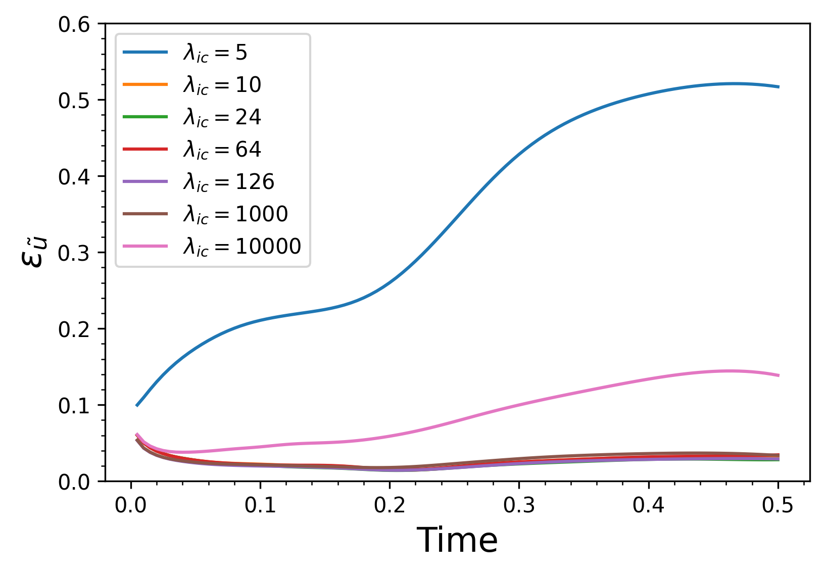
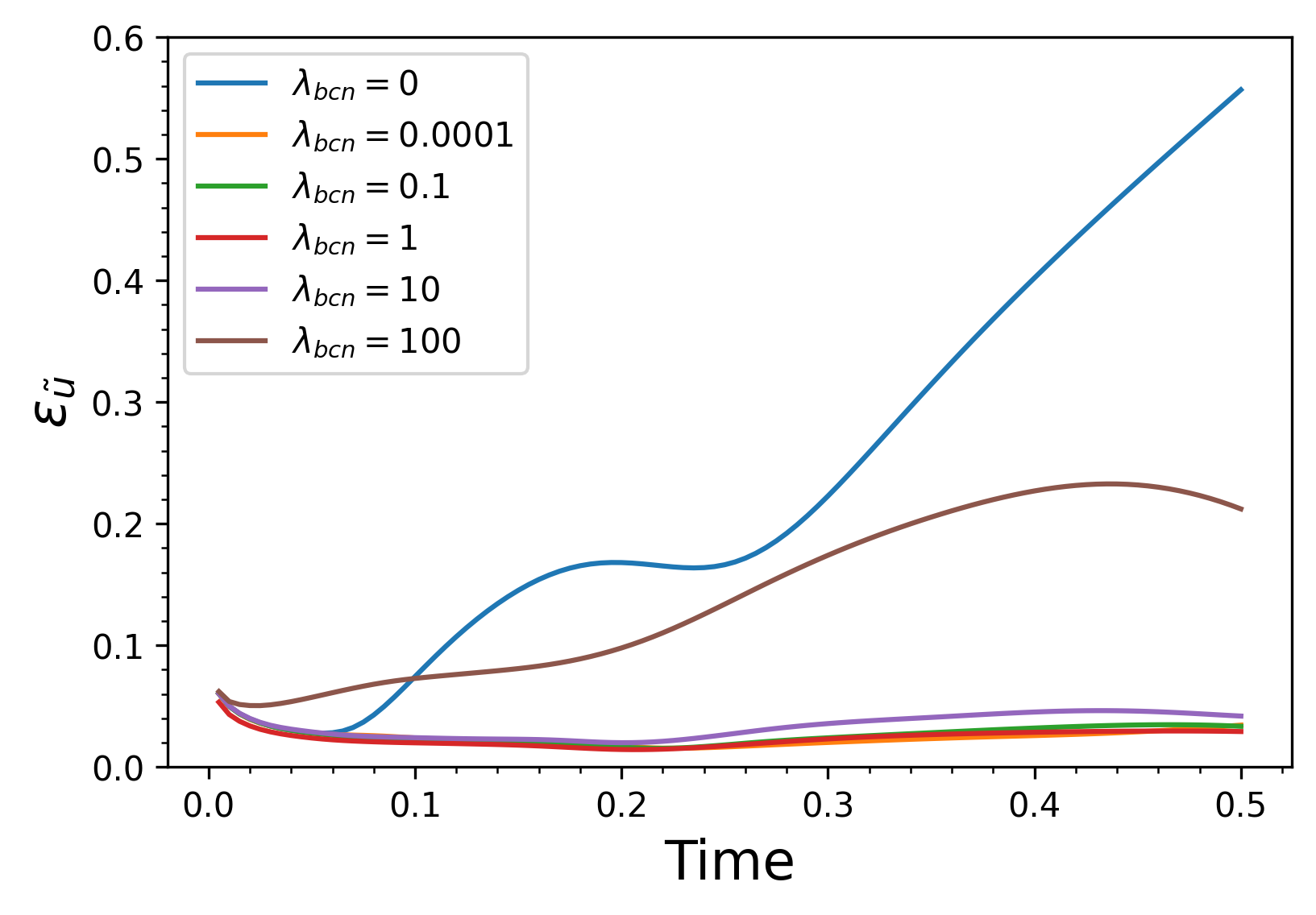
Figure 5: (a) Relative L2subscript𝐿2L_{2} errors Ξ΅usubscriptπœ€π‘’\varepsilon_{u} in the PINN solutions as functions of time with for different Ξ»i​c=Ξ»b​dsubscriptπœ†π‘–π‘subscriptπœ†π‘π‘‘\lambda_{ic}=\lambda_{bd} values. The other weights are Ξ»r​e​s=Ξ»b​c​n=1subscriptπœ†π‘Ÿπ‘’π‘ subscriptπœ†π‘π‘π‘›1\lambda_{res}=\lambda_{bcn}=1. (b) Relative L2subscript𝐿2L_{2} errors Ξ΅usubscriptπœ€π‘’\varepsilon_{u} in the PINN solutions as functions of time for different values of Ξ»b​c​nsubscriptπœ†π‘π‘π‘›\lambda_{bcn}. The other weights are Ξ»r​e​s=1subscriptπœ†π‘Ÿπ‘’π‘ 1\lambda_{res}=1 and Ξ»i​c=Ξ»b​d=126subscriptπœ†π‘–π‘subscriptπœ†π‘π‘‘126\lambda_{ic}=\lambda_{bd}=126.

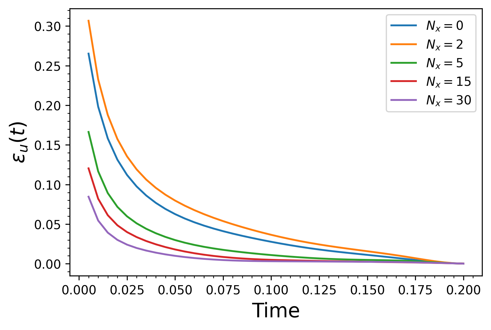
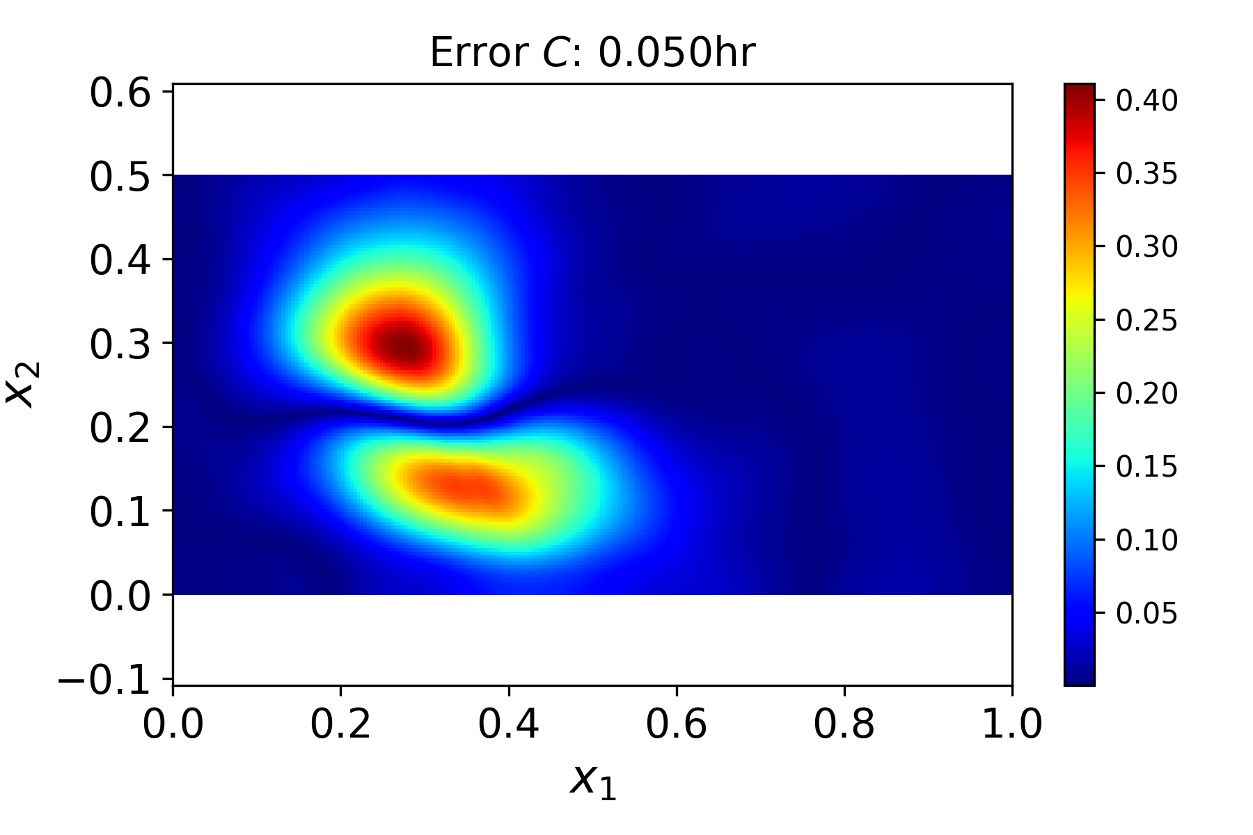
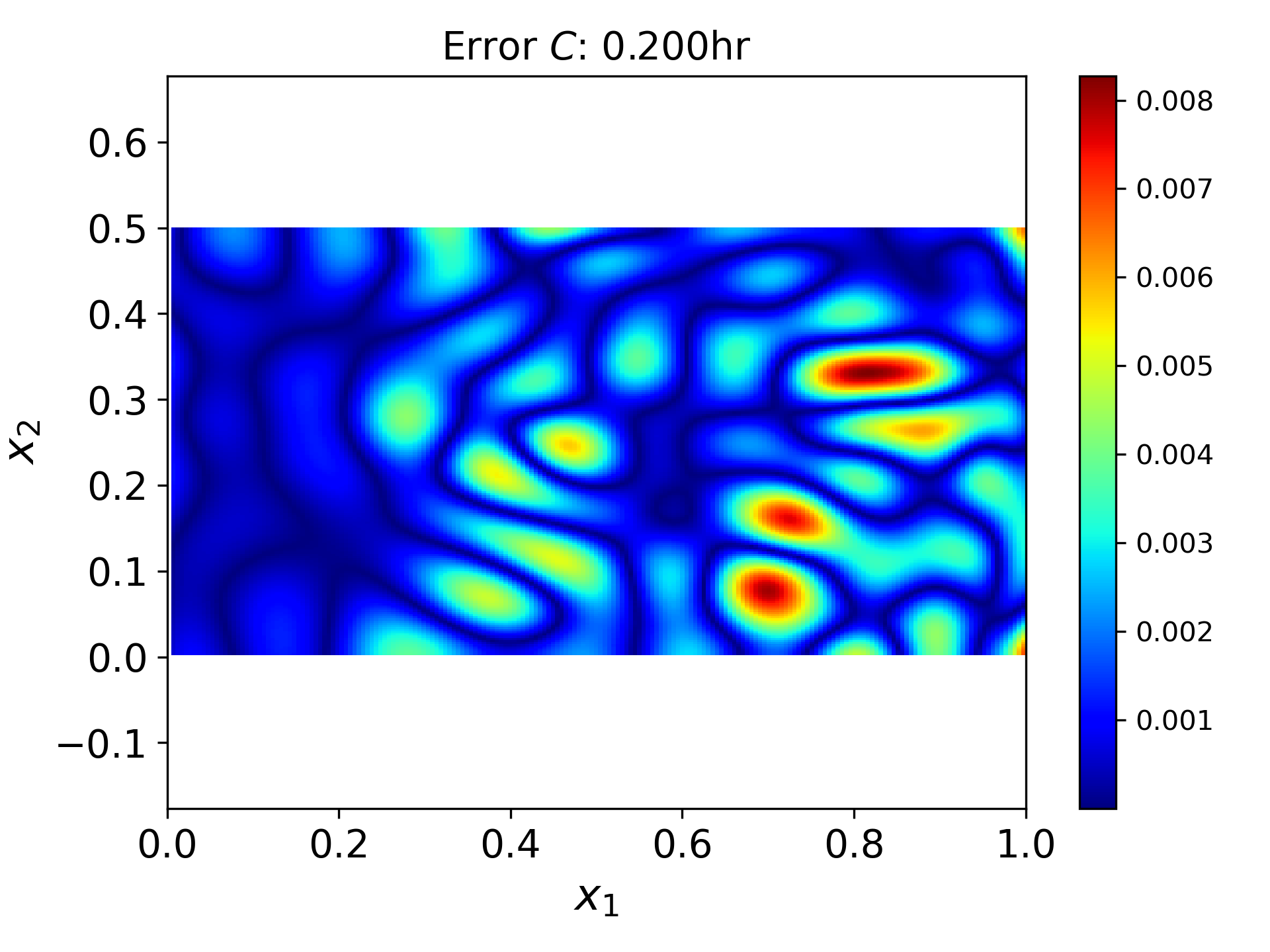
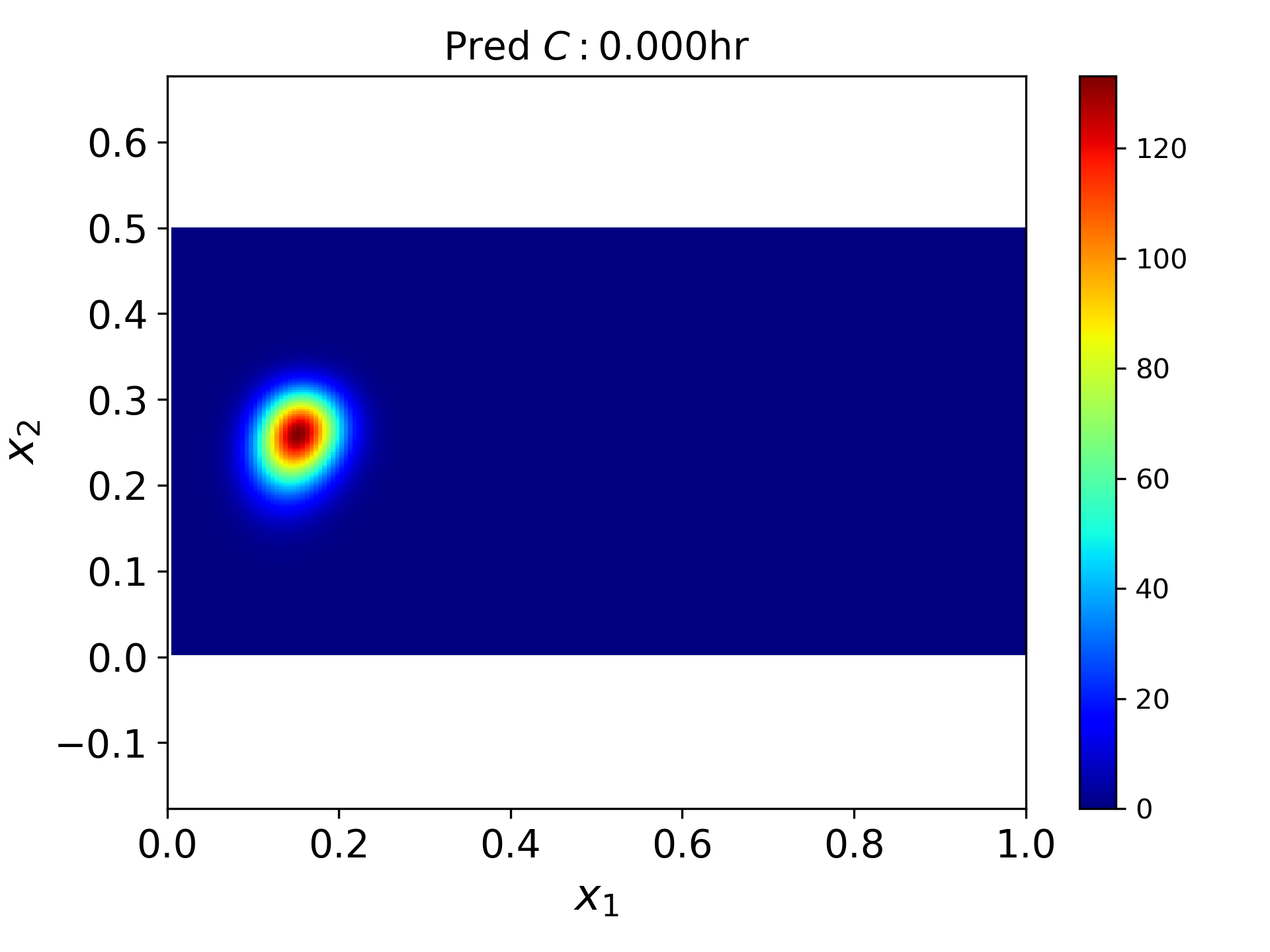
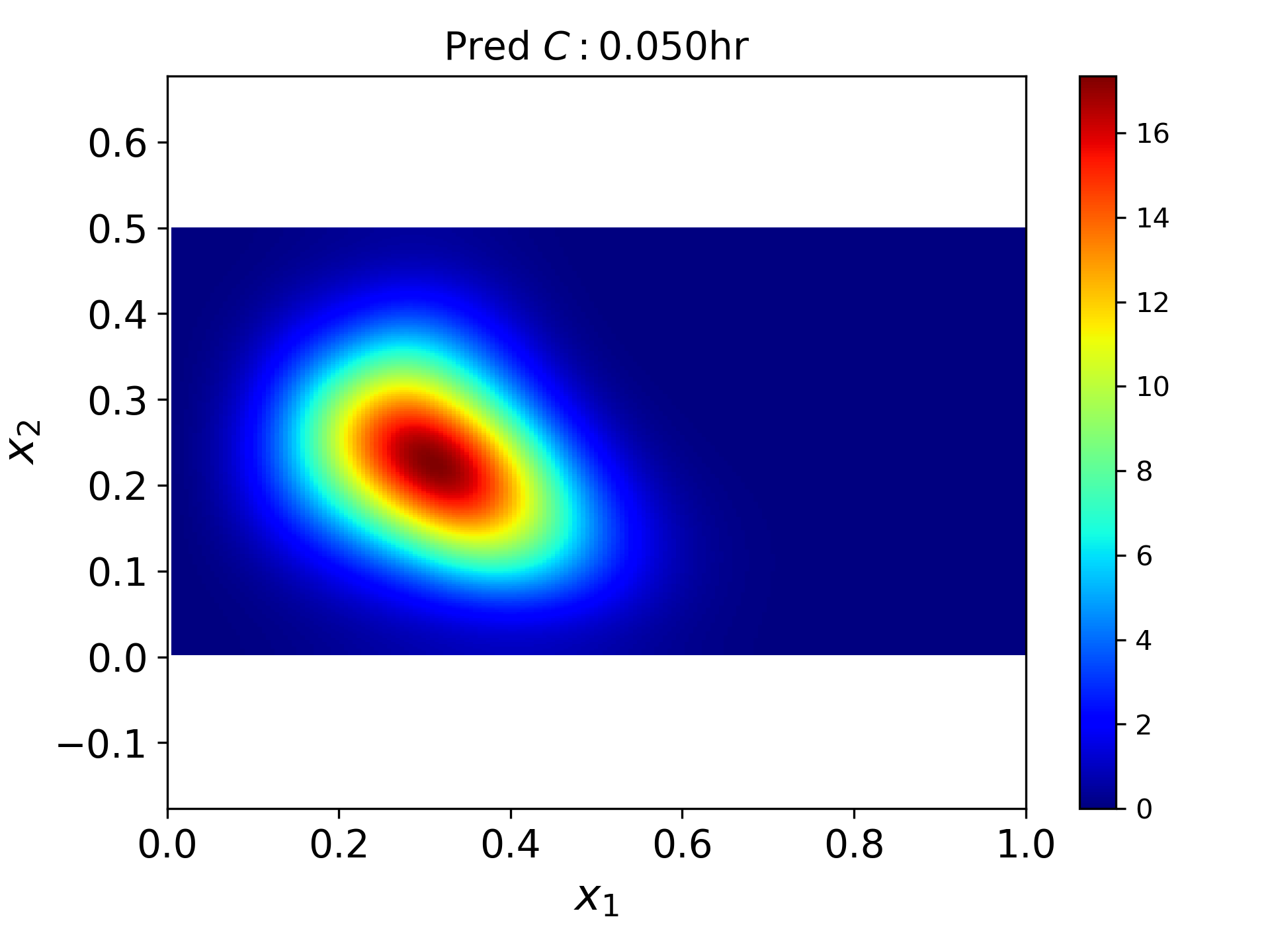
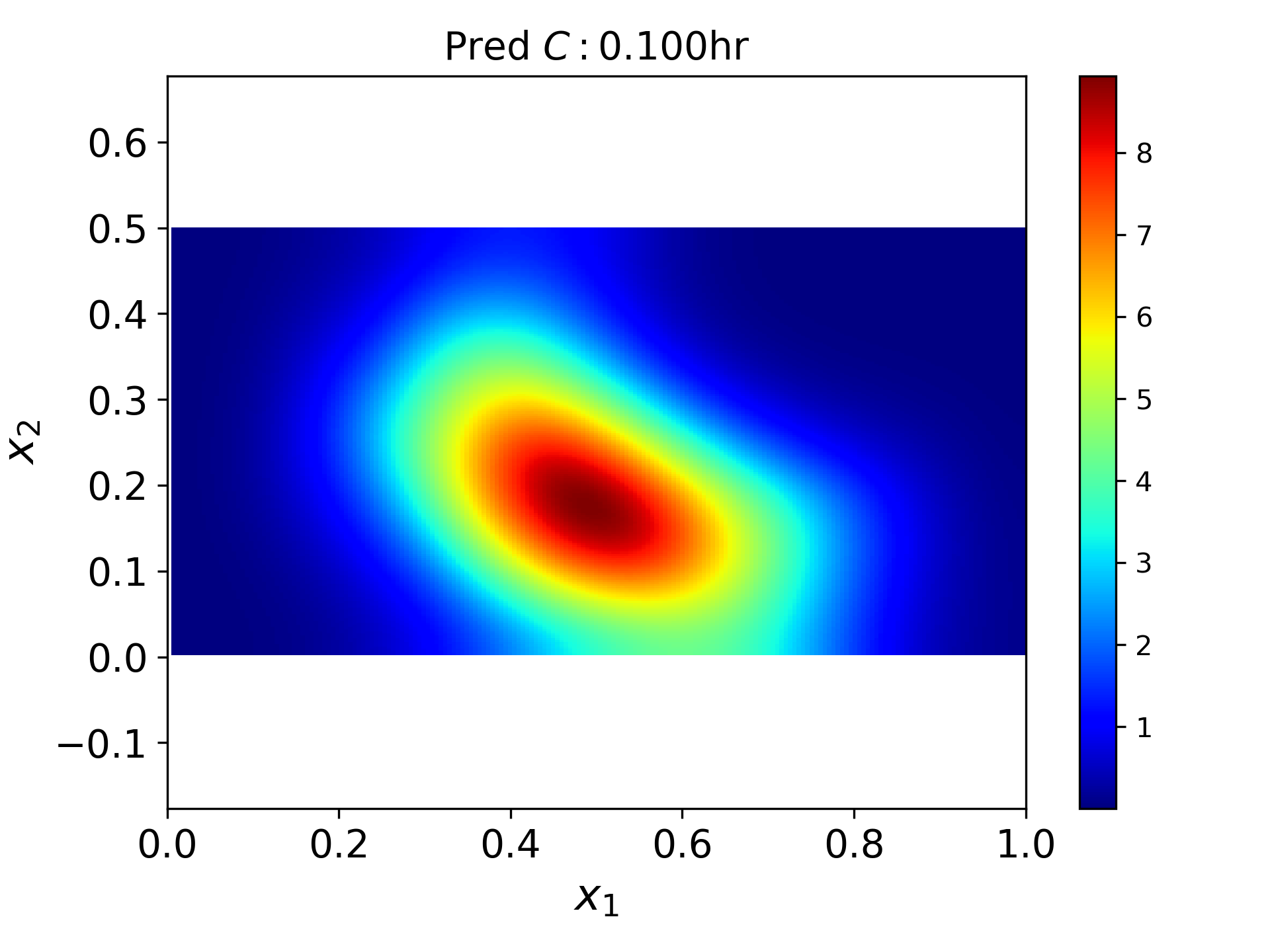
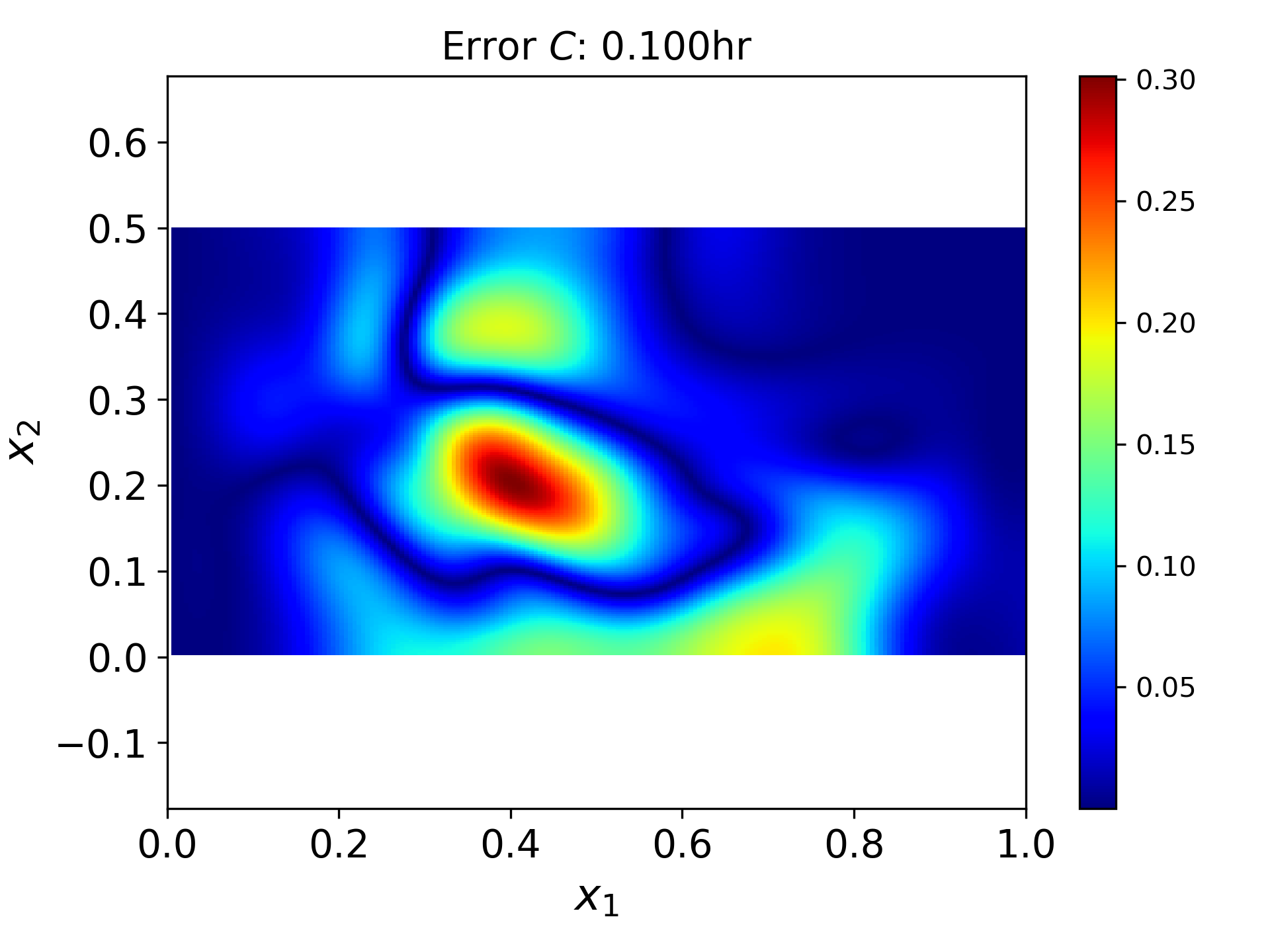
Figure 5(a) shows the relative L2subscript𝐿2L_{2} errors Ξ΅u​(t)subscriptπœ€π‘’π‘‘\varepsilon_{u}(t) for Ξ»b​c​n=1subscriptπœ†π‘π‘π‘›1\lambda_{bcn}=1 and values of Ξ»i​c=Ξ»b​c​dsubscriptπœ†π‘–π‘subscriptπœ†π‘π‘π‘‘\lambda_{ic}=\lambda_{bcd} in the range [5,10000]. In this figure, the largest error (exceeding 50%) corresponds to Ξ»i​c=5subscriptπœ†π‘–π‘5\lambda_{ic}=5. Not shown here, the error exceeds 100% for Ξ»i​c=1subscriptπœ†π‘–π‘1\lambda_{ic}=1. For Ξ»i​c=10000subscriptπœ†π‘–π‘10000\lambda_{ic}=10000, the relative error is about 12%. However, for Ξ»i​csubscriptπœ†π‘–π‘\lambda_{ic} in the range [10,1000]101000[10,1000], the PINN errors do not exceed 6% and are practically independent of Ξ»i​csubscriptπœ†π‘–π‘\lambda_{ic} (vary by less than 1%). We find that the smallest error is achieved at Ξ»i​c=126subscriptπœ†π‘–π‘126\lambda_{ic}=126. We plot the concentration field and the absolute point errors at selected time snapshots for this case in Fig 12.

The value estimated by the proposed criterion in Eq (36) is Ξ»i​c=24subscriptπœ†π‘–π‘24\lambda_{ic}=24, which is within the range of Ξ»i​csubscriptπœ†π‘–π‘\lambda_{ic} that produces an accurate solution. The error obtained with Ξ»i​c=24subscriptπœ†π‘–π‘24\lambda_{ic}=24 is also shown in Figure 5(a) and is very close to the smallest error obtained with Ξ»i​c=126subscriptπœ†π‘–π‘126\lambda_{ic}=126. In the following examples, we set Ξ»i​c=126subscriptπœ†π‘–π‘126\lambda_{ic}=126.

Figure 5(b) shows the relative L2subscript𝐿2L_{2} errors Ξ΅u​(t)subscriptπœ€π‘’π‘‘\varepsilon_{u}(t) for Ξ»b​c​nsubscriptπœ†π‘π‘π‘›\lambda_{bcn} varying in the range [0,100]. Other weights are set to Ξ»i​c=Ξ»b​c​d=126subscriptπœ†π‘–π‘subscriptπœ†π‘π‘π‘‘126\lambda_{ic}=\lambda_{bcd}=126 and Ξ»r​e​s=1subscriptπœ†π‘Ÿπ‘’π‘ 1\lambda_{res}=1. For Ξ»b​c​n=0subscriptπœ†π‘π‘π‘›0\lambda_{bcn}=0 and 100, the maximum relative errors are 56% and 24%, respectively. The smallest errors are for Ξ»b​c​nsubscriptπœ†π‘π‘π‘›\lambda_{bcn} in the [0.0001,1] range. In this range, the errors do not exceed 6% and are practically independent of Ξ»b​c​nsubscriptπœ†π‘π‘π‘›\lambda_{bcn}.

These results agree with the Ξ»b​c​nsubscriptπœ†π‘π‘π‘›\lambda_{bcn} estimate Ξ»b​c​n=κ​λi​csubscriptπœ†π‘π‘π‘›πœ…subscriptπœ†π‘–π‘\lambda_{bcn}=\kappa\lambda_{ic} (ΞΊ<<1much-less-thanπœ…1\kappa<<1).

4.2 Effect of the neural network size and the number of residual points

In this section, the dependence of PINN accuracy on the neural network size and the number of residual points is investigated. In all simulations, the weights are set to Ξ»i​c=Ξ»b​c​d=126subscriptπœ†π‘–π‘subscriptπœ†π‘π‘π‘‘126\lambda_{ic}=\lambda_{bcd}=126 and Ξ»r​e​s=Ξ»b​c​n=1subscriptπœ†π‘Ÿπ‘’π‘ subscriptπœ†π‘π‘π‘›1\lambda_{res}=\lambda_{bcn}=1. First, we study the PINN error as the function of the number of neurons per hidden layer Nnsubscript𝑁𝑛N_{n}. The number of hidden layers is kept at 5, and 100,000 residual points are distributed adaptively in time. To facilitate the comparison between different cases, we show the averaged-over-time relative L2 error

Ξ΅u~=βˆ‘i=1Ntβˆ‘j=1Nt​o​t[u~​(𝐱j,ti)βˆ’u^​(𝐱j,ti)]2βˆ‘i=1Ntβˆ‘j=1Nt​o​tu~​(𝐱j,ti)2,subscriptπœ€~𝑒superscriptsubscript𝑖1subscript𝑁𝑑superscriptsubscript𝑗1subscriptπ‘π‘‘π‘œπ‘‘superscriptdelimited-[]~𝑒subscript𝐱𝑗subscript𝑑𝑖^𝑒subscript𝐱𝑗subscript𝑑𝑖2superscriptsubscript𝑖1subscript𝑁𝑑superscriptsubscript𝑗1subscriptπ‘π‘‘π‘œπ‘‘~𝑒superscriptsubscript𝐱𝑗subscript𝑑𝑖2\varepsilon_{\tilde{u}}=\sqrt{\frac{\sum_{i=1}^{N_{t}}\sum_{j=1}^{N_{tot}}\left[\tilde{u}(\mathbf{x}_{j},t_{i})-\hat{u}(\mathbf{x}_{j},t_{i})\right]^{2}}{\sum_{i=1}^{N_{t}}\sum_{j=1}^{N_{tot}}\tilde{u}(\mathbf{x}_{j},t_{i})^{2}}}, (45)

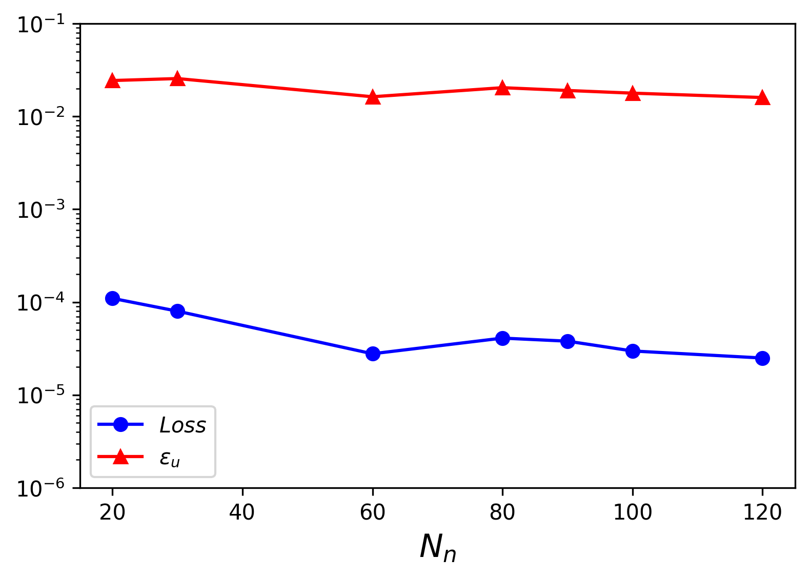
where Ntsubscript𝑁𝑑N_{t} is the number of time snapshots in the simulation. Figure 6(a) shows Ξ΅u~subscriptπœ€~𝑒\varepsilon_{\tilde{u}} and the magnitude of the PINN loss as functions of Nnsubscript𝑁𝑛N_{n}. For Nnsubscript𝑁𝑛N_{n} ranging from 20 to 120, Ξ΅u~subscriptπœ€~𝑒\varepsilon_{\tilde{u}} and the loss are decreasing with increasing Nnsubscript𝑁𝑛N_{n}. However, the dependence on Nnsubscript𝑁𝑛N_{n} is small. We find that Ξ΅u~subscriptπœ€~𝑒\varepsilon_{\tilde{u}} is almost the same for Nn=60subscript𝑁𝑛60N_{n}=60 and 120. The comparison of this figure with Figure 4 reveals the importance of the proposed normalization of the ADE because the DNN size of five layers and Nn=60subscript𝑁𝑛60N_{n}=60 is sufficient to produce an accurate PINN solution of the normalized ADE. However, this leads to a highly inaccurate solution when applied to a non-normalized ADE.

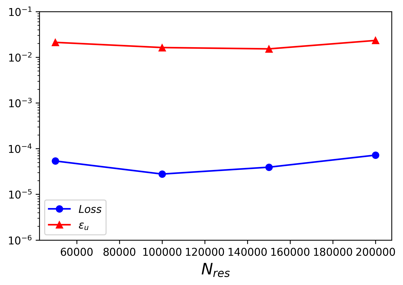
Next, we study the effect of the number of residual points on the PINN error. Here, we fix the size of DNN at five hidden layers with Nn=60subscript𝑁𝑛60N_{n}=60 and consider the number of residual points in the range [50000, 200000].
Refer to caption
(a)
Refer to caption
(b)
Figure 6: (a) The loss function at the end of the training and the average-over-time relative L2 error as functions of Nnsubscript𝑁𝑛N_{n}. Nr​e​s=100,000subscriptπ‘π‘Ÿπ‘’π‘ 100000N_{res}=100,000. (b) The loss at the end of the training and the average-over-time relative L2 error as functions of Nr​e​ssubscriptπ‘π‘Ÿπ‘’π‘ N_{res}. Nn=60subscript𝑁𝑛60N_{n}=60.

The Ξ΅u~subscriptπœ€~𝑒\varepsilon_{\tilde{u}} error and PINN loss as functions of Nr​e​ssubscriptπ‘π‘Ÿπ‘’π‘ N_{res} are shown in Figure 6(b). For Nr​e​ssubscriptπ‘π‘Ÿπ‘’π‘ N_{res} in the considered range, the error is practically independent of Nr​e​ssubscriptπ‘π‘Ÿπ‘’π‘ N_{res} with the smallest errors obtained for Nr​e​s=100,000subscriptπ‘π‘Ÿπ‘’π‘ 100000N_{res}=100,000 and 160,000. The dependence of the loss on Nr​e​ssubscriptπ‘π‘Ÿπ‘’π‘ N_{res} is weak with the smallest values of the loss terms obtained for Nr​e​s=100,000subscriptπ‘π‘Ÿπ‘’π‘ 100000N_{res}=100,000. A small increase in the value of the loss with increasing Nr​e​ssubscriptπ‘π‘Ÿπ‘’π‘ N_{res} is expected because the DNN approximation of the solution is not exact.

4.3 Parameter and state estimation

In Sections 4.1 and 4.2, the PINN solutions were obtained without any measurements of u𝑒u except for the initial and boundary conditions. However, the parameter and state measurements can sometimes be available and can easily be included or β€œassimilated” in the PINN formulation of the PDE solution. In the following, we show that data assimilation can help accurately estimate u𝑒u even when the velocity field 𝐯𝐯\mathbf{v} is not fully known. Here, we assume that NKsubscript𝑁𝐾N_{K}, Nhsubscriptπ‘β„ŽN_{h}, and Nusubscript𝑁𝑒N_{u} measurements of the K​(𝒙)𝐾𝒙K(\bm{x}), h​(𝒙)β„Žπ’™h(\bm{x}), and u​(𝒙,t)𝑒𝒙𝑑u(\bm{x},t) fields are available. Because of the incomplete knowledge of the K𝐾K field, 𝐯𝐯\mathbf{v} cannot be exactly found from the Darcy equation. However, the solutions of the Darcy and ADE equations can be found by formulating the joint PINN data assimilation problem as

Ξ±βˆ—,Ξ²βˆ—,Ξ³βˆ—=minΞ±,Ξ²,γ⁑{L~​(Ξ±,Ξ²,Ξ³)=L~D​a​(Ξ±,Ξ²)+L~A​D​(Ξ±,Ξ²,Ξ³)+L~d​a​t​a​(Ξ±,Ξ²,Ξ³)}superscript𝛼superscript𝛽superscript𝛾subscript𝛼𝛽𝛾~𝐿𝛼𝛽𝛾subscript~πΏπ·π‘Žπ›Όπ›½subscript~𝐿𝐴𝐷𝛼𝛽𝛾subscript~πΏπ‘‘π‘Žπ‘‘π‘Žπ›Όπ›½π›Ύ\alpha^{*},\beta^{*},\gamma^{*}=\min_{\alpha,\beta,\gamma}\Big{\{}\tilde{L}(\alpha,\beta,\gamma)=\tilde{L}_{Da}(\alpha,\beta)+\tilde{L}_{AD}(\alpha,\beta,\gamma)+\tilde{L}_{data}(\alpha,\beta,\gamma)\Big{\}} (46)

where α𝛼\alpha, β𝛽\beta, and γ𝛾\gamma are parameters of the k^^π‘˜\hat{k}, h^^β„Ž\hat{h}, and u^^𝑒\hat{u} DNNs,

L~D​a​(Ξ±,Ξ²)subscript~πΏπ·π‘Žπ›Όπ›½\displaystyle\tilde{L}_{Da}(\alpha,\beta) =\displaystyle= Ξ»b​c​nD​aNb​c​nD​aβˆ‘n=1Nb​c​nD​a[βˆ‚h^​(𝐱;Ξ²)βˆ‚π±|𝐱=𝐱nβ‹…π§βˆ’q~(𝐱n)]2\displaystyle\frac{\lambda_{bcn}^{Da}}{N_{bcn}^{Da}}\sum_{n=1}^{N_{bcn}^{Da}}\left[\frac{\partial\hat{h}(\mathbf{x};\beta)}{\partial\mathbf{x}}\Big{\rvert}_{\mathbf{x}=\mathbf{x}_{n}}\cdot\mathbf{n}-\tilde{q}(\mathbf{x}_{n})\right]^{2}
+\displaystyle+ Ξ»b​c​dD​aNb​c​dD​aβ€‹βˆ‘n=1Nb​c​dD​a[h^​(𝐱n;Ξ²)βˆ’h~​(𝐱n)]2+Ξ»r​e​sD​aNr​e​sD​aβ€‹βˆ‘n=1Nr​e​sD​a[β„›~k^,h^​(𝐱n;Ξ±,Ξ²)]2superscriptsubscriptπœ†π‘π‘π‘‘π·π‘Žsuperscriptsubscriptπ‘π‘π‘π‘‘π·π‘Žsuperscriptsubscript𝑛1superscriptsubscriptπ‘π‘π‘π‘‘π·π‘Žsuperscriptdelimited-[]^β„Žsubscript𝐱𝑛𝛽~β„Žsubscript𝐱𝑛2superscriptsubscriptπœ†π‘Ÿπ‘’π‘ π·π‘Žsuperscriptsubscriptπ‘π‘Ÿπ‘’π‘ π·π‘Žsuperscriptsubscript𝑛1superscriptsubscriptπ‘π‘Ÿπ‘’π‘ π·π‘Žsuperscriptdelimited-[]subscript~β„›^π‘˜^β„Žsubscript𝐱𝑛𝛼𝛽2\displaystyle\frac{\lambda_{bcd}^{Da}}{N_{bcd}^{Da}}\sum_{n=1}^{N_{bcd}^{Da}}[\hat{h}(\mathbf{x}_{n};\beta)-\tilde{h}(\mathbf{x}_{n})]^{2}+\frac{\lambda_{res}^{Da}}{N_{res}^{Da}}\sum_{n=1}^{N_{res}^{Da}}[\tilde{\mathcal{R}}_{\hat{k},\hat{h}}(\mathbf{x}_{n};\alpha,\beta)]^{2}

is the loss term enforcing constraints due to the Darcy flow equation, and

L~d​a​t​a​(Ξ±,Ξ²,Ξ³)subscript~πΏπ‘‘π‘Žπ‘‘π‘Žπ›Όπ›½π›Ύ\displaystyle\tilde{L}_{data}(\alpha,\beta,\gamma) =\displaystyle= Ξ»d​a​t​aNx​Ntβ€‹βˆ‘n=1Nxβˆ‘m=1Nt(u^​(𝐱nu,tmu;Ξ³)βˆ’uβˆ—β€‹(𝐱nu,tm))2subscriptπœ†π‘‘π‘Žπ‘‘π‘Žsubscript𝑁π‘₯subscript𝑁𝑑superscriptsubscript𝑛1subscript𝑁π‘₯superscriptsubscriptπ‘š1subscript𝑁𝑑superscript^𝑒superscriptsubscript𝐱𝑛𝑒superscriptsubscriptπ‘‘π‘šπ‘’π›Ύsuperscript𝑒superscriptsubscript𝐱𝑛𝑒subscriptπ‘‘π‘š2\displaystyle\frac{\lambda_{data}}{N_{x}N_{t}}\sum_{n=1}^{N_{x}}\sum_{m=1}^{N_{t}}(\hat{u}(\mathbf{x}_{n}^{u},t_{m}^{u};\gamma)-u^{*}(\mathbf{x}_{n}^{u},t_{m}))^{2}
+\displaystyle+ Ξ»d​a​t​aNKβˆ‘n=1NK(K^(𝐱nk,;Ξ±)βˆ’Kβˆ—(𝐱nk))2+Ξ»d​a​t​aNhβˆ‘n=1Nh(h^(𝐱nh;Ξ²)βˆ’hβˆ—(𝐱nh))2\displaystyle\frac{\lambda_{data}}{N_{K}}\sum_{n=1}^{N_{K}}(\hat{K}(\mathbf{x}_{n}^{k},;\alpha)-K^{*}(\mathbf{x}_{n}^{k}))^{2}+\frac{\lambda_{data}}{N_{h}}\sum_{n=1}^{N_{h}}(\hat{h}(\mathbf{x}_{n}^{h};\beta)-h^{*}(\mathbf{x}_{n}^{h}))^{2}

is the loss term enforcing the measurements of u𝑒u, K𝐾K, and hβ„Žh on the PDE solutions. The form of L~A​D​(Ξ±,Ξ²,Ξ³)subscript~𝐿𝐴𝐷𝛼𝛽𝛾\tilde{L}_{AD}(\alpha,\beta,\gamma) is identical to Eq (3.2) except that α𝛼\alpha and β𝛽\beta are now unknown parameters.

In Eq (4.3), β„›~k^,h^​(𝐱n;Ξ±,Ξ²)=βˆ‡~β‹…(k^β€‹βˆ‡~​h^)subscript~β„›^π‘˜^β„Žsubscript𝐱𝑛𝛼𝛽⋅~βˆ‡^π‘˜~βˆ‡^β„Ž\tilde{\mathcal{R}}_{\hat{k},\hat{h}}(\mathbf{x}_{n};\alpha,\beta)=\tilde{\nabla}\cdot(\hat{k}\tilde{\nabla}\hat{h}) is the residual of the normalized Darcy equation (28). The Dirichlet and Neumann BCs of the Darcy flow equation are enforced at the Nb​c​dD​a=Nb​c​nxsubscriptsuperscriptπ‘π·π‘Žπ‘π‘π‘‘subscriptsuperscript𝑁π‘₯𝑏𝑐𝑛N^{Da}_{bcd}=N^{x}_{bcn} and Nb​c​nD​a=Nb​c​dxsubscriptsuperscriptπ‘π·π‘Žπ‘π‘π‘›subscriptsuperscript𝑁π‘₯𝑏𝑐𝑑N^{Da}_{bcn}=N^{x}_{bcd} number of points, respectively.

In Eq (4.3), uβˆ—β€‹(𝐱nu,tm)superscript𝑒superscriptsubscript𝐱𝑛𝑒subscriptπ‘‘π‘šu^{*}(\mathbf{x}_{n}^{u},t_{m}) is a normalized measurement of u𝑒u at the location 𝐱nusuperscriptsubscript𝐱𝑛𝑒\mathbf{x}_{n}^{u} (n=1,…,Nx𝑛1…subscript𝑁π‘₯n=1,...,N_{x}) and time tmsubscriptπ‘‘π‘št_{m} (m=1,…,Ntπ‘š1…subscript𝑁𝑑m=1,...,N_{t}). We assume that uβˆ—superscript𝑒u^{*} is sampled uniformly in the time interval (0,T]0𝑇(0,T] and that the number of uβˆ—superscript𝑒u^{*} measurements at each spatial location is Nt=100subscript𝑁𝑑100N_{t}=100, resulting in the total number of u𝑒u samples Nu=NxΓ—Ntsubscript𝑁𝑒subscript𝑁π‘₯subscript𝑁𝑑N_{u}=N_{x}\times N_{t}. The sampling locations for uβˆ—superscript𝑒u^{*} are selected randomly in space. Similarly, Kβˆ—β€‹(𝐱nk)superscript𝐾superscriptsubscriptπ±π‘›π‘˜K^{*}(\mathbf{x}_{n}^{k}) and hβˆ—β€‹(𝐱nh)superscriptβ„Žsuperscriptsubscriptπ±π‘›β„Žh^{*}(\mathbf{x}_{n}^{h}) are the normalized measurements of K𝐾K and hβ„Žh at the locations 𝐱nKsuperscriptsubscript𝐱𝑛𝐾\mathbf{x}_{n}^{K} and 𝐱nhsuperscriptsubscriptπ±π‘›β„Ž\mathbf{x}_{n}^{h}, respectively. In the following examples, we set Nk=Nh=20subscriptπ‘π‘˜subscriptπ‘β„Ž20N_{k}=N_{h}=20, and vary Nxsubscript𝑁π‘₯N_{x} in the range [0,60]. The number of residual points in the Darcy and ADE residual losses are Nr​e​sD​a=10,000subscriptsuperscriptπ‘π·π‘Žπ‘Ÿπ‘’π‘ 10000N^{Da}_{res}=10,000 and Nr​e​sA​D=60,000subscriptsuperscriptπ‘π΄π·π‘Ÿπ‘’π‘ 60000N^{AD}_{res}=60,000, respectively. The residual points for the Darcy equation are selected using the LHS scheme. The points for enforcing the initial and boundary conditions and the residuals in L~A​Dsubscript~𝐿𝐴𝐷\tilde{L}_{AD} are selected as in the forward ADE problem. The magnitude of the L~d​a​t​asubscript~πΏπ‘‘π‘Žπ‘‘π‘Ž\tilde{L}_{data} term is the same as that of the L~i​csubscript~𝐿𝑖𝑐\tilde{L}_{ic} term in Eq (31). Therefore, we set set Ξ»d​a​t​a=Ξ»i​csubscriptπœ†π‘‘π‘Žπ‘‘π‘Žsubscriptπœ†π‘–π‘\lambda_{data}=\lambda_{ic}. Following [22], the weights in the loss term in Eq (4.3) are selected as Ξ»b​c​nD​a=Ξ»b​c​dD​a=Ξ»r​e​sD​a=1superscriptsubscriptπœ†π‘π‘π‘›π·π‘Žsuperscriptsubscriptπœ†π‘π‘π‘‘π·π‘Žsuperscriptsubscriptπœ†π‘Ÿπ‘’π‘ π·π‘Ž1\lambda_{bcn}^{Da}=\lambda_{bcd}^{Da}=\lambda_{res}^{Da}=1. Finally, the k^^π‘˜\hat{k}, h^^β„Ž\hat{h}, and u^^𝑒\hat{u} DNNs are set to five hidden layers with 60 neurons per layer.

Figure 7(a) presents the relative PINN error in the estimated u𝑒u field as a function of time for different values of Nxsubscript𝑁π‘₯N_{x}. It can be seen that the error decreases with increasing Nxsubscript𝑁π‘₯N_{x}, with the the maximum error close to 70% for Nx=0subscript𝑁π‘₯0N_{x}=0 and less than 5% for Nx=60subscript𝑁π‘₯60N_{x}=60. Figure 7(b) presents the relative L2 errors in the estimated hydraulic conductivity and the velocity magnitude as functions of Nxsubscript𝑁π‘₯N_{x}. The error in the estimated K𝐾K is reduced from over 43% for Nx=0subscript𝑁π‘₯0N_{x}=0 to less than 8% for Nx=60subscript𝑁π‘₯60N_{x}=60. The error in the estimated velocity decreases from 20% for Nx=0subscript𝑁π‘₯0N_{x}=0 to less that 8% for Nx=60subscript𝑁π‘₯60N_{x}=60. We note that the error in the estimated u𝑒u field obtained with Nx=60subscript𝑁π‘₯60N_{x}=60 u𝑒u measurements is similar to the error in the estimated u𝑒u with the fully known velocity field in Section 4.2. These results show the ability of the PINN method to assimilate static and dynamic data for the state and parameter estimation.
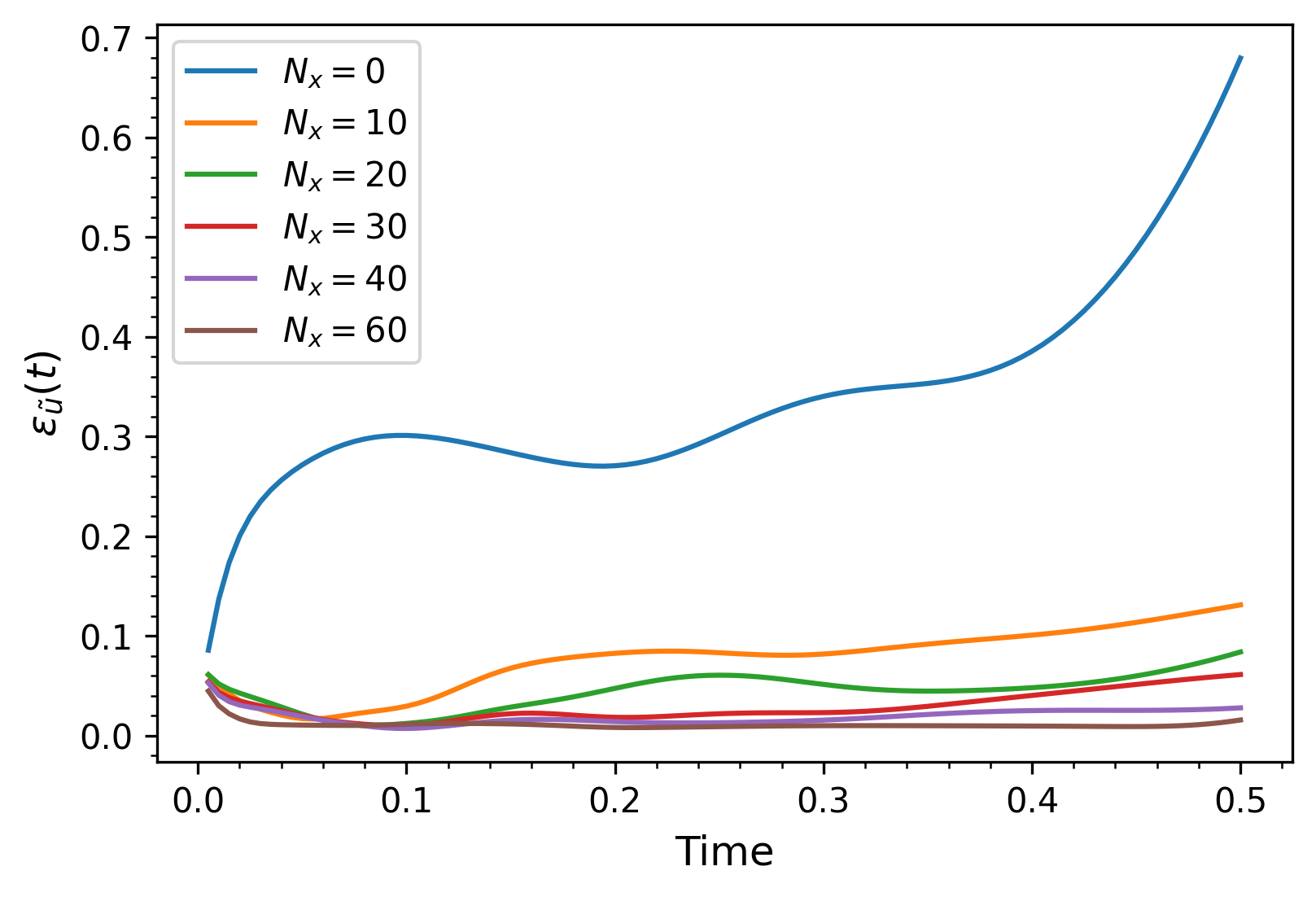
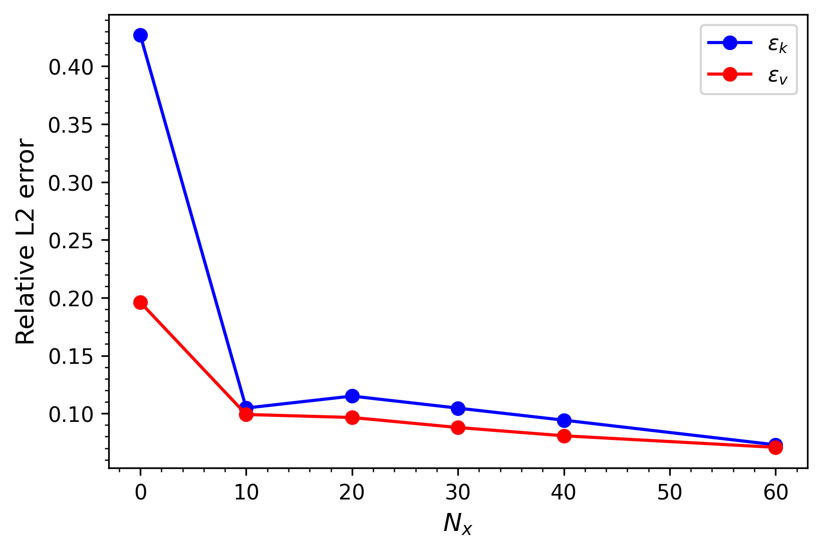
Refer to caption
(a)
Refer to caption
(b)
Figure 7: (a) Relative L2subscript𝐿2L_{2} errors in the PINN u^^𝑒\hat{u} solutions versus time for different Nxsubscript𝑁π‘₯N_{x}, the number of concentration measurements. Nk=Nh=20subscriptπ‘π‘˜subscriptπ‘β„Ž20N_{k}=N_{h}=20, Nr​e​sD​a=10,000subscriptsuperscriptπ‘π·π‘Žπ‘Ÿπ‘’π‘ 10000N^{Da}_{res}=10,000, and Nr​e​sA​D=60,000subscriptsuperscriptπ‘π΄π·π‘Ÿπ‘’π‘ 60000N^{AD}_{res}=60,000. (b) Relative L2subscript𝐿2L_{2} errors in the PINN estimates of conductivity (Ξ΅vsubscriptπœ€π‘£\varepsilon_{v}) and the magnitude of velocity (Ξ΅vsubscriptπœ€π‘£\varepsilon_{v}) as functions of Nxsubscript𝑁π‘₯N_{x}.

5 PINN for backward ADE

5.1 DNN with identity activation function in the last layer

Here, we investigate the accuracy of PINN for solving backward ADEs, which can arise in the source identification problems. We consider the backward ADE, which before normalization is given by Eq (8) subject to the terminal condition (10). The terminal time T𝑇T is set to 0.2. At T=0.2𝑇0.2T=0.2, approximately 70% of the released mass remains in the computational domain ΩΩ\Omega. The concentration field U​(𝐱)π‘ˆπ±U(\mathbf{x}) at the terminal time is given by by the MT3DMS solution of the forward ADE at t=T𝑑𝑇t=T and is shown in Figure 8.

As for the forward problem, we normalize the backward ADE by introducing the dimensionless variable u~​(𝐱,t)=u​(𝐱,t)g​(t)~𝑒𝐱𝑑𝑒𝐱𝑑𝑔𝑑\tilde{u}(\mathbf{x},t)=\frac{u(\mathbf{x},t)}{g(t)} where g​(t)𝑔𝑑g(t) is defined by Eq (24). This leads to the dimensionless form of the backward ADE (26) subject to the dimensionless boundary conditions (27) and the terminal condition

u~​(𝐱~,t~=T~)=U~​(𝐱~).~𝑒~𝐱~𝑑~𝑇~π‘ˆ~𝐱\tilde{u}(\tilde{\mathbf{x}},\tilde{t}=\tilde{T})=\tilde{U}(\tilde{\mathbf{x}}). (49)

The proposed normalization assumes that the release time (t=0𝑑0t=0) and the released mass (M=1𝑀1M=1) are known. Also, this normalization assumes that the plume at the time of release has the Gaussian shape with the known standard deviation Ξ΅πœ€\varepsilon. The location of the plume at the time of release is treated as an unknown.

The PINN solution of the dimensionless backward PDE is found by minimizing the loss function:

L~u^​(Ξ³)=Ξ»t​cΓ—L~t​c​(Ξ³)+Ξ»b​c​nΓ—L~b​c​n​(Ξ³)+Ξ»b​c​dΓ—L~b​c​d​(Ξ³)+Ξ»r​e​sΓ—L~r​e​s​(Ξ³)subscript~𝐿^𝑒𝛾subscriptπœ†π‘‘π‘subscript~𝐿𝑑𝑐𝛾subscriptπœ†π‘π‘π‘›subscript~𝐿𝑏𝑐𝑛𝛾subscriptπœ†π‘π‘π‘‘subscript~𝐿𝑏𝑐𝑑𝛾subscriptπœ†π‘Ÿπ‘’π‘ subscript~πΏπ‘Ÿπ‘’π‘ π›Ύ\tilde{L}_{\hat{u}}(\gamma)=\lambda_{tc}\times\tilde{L}_{tc}(\gamma)+\lambda_{bcn}\times\tilde{L}_{bcn}(\gamma)+\lambda_{bcd}\times\tilde{L}_{bcd}(\gamma)+\lambda_{res}\times\tilde{L}_{res}(\gamma) (50)

Here, the weights L~b​c​nsubscript~𝐿𝑏𝑐𝑛\tilde{L}_{bcn}, L~b​c​dsubscript~𝐿𝑏𝑐𝑑\tilde{L}_{bcd}, and L~r​e​ssubscript~πΏπ‘Ÿπ‘’π‘ \tilde{L}_{res} are the same as in the loss function for the normalized forward ADE. The term L~t​csubscript~𝐿𝑑𝑐\tilde{L}_{tc} enforces the terminal condition (49) and has the form:

L~t​c=1Nt​cβˆ‘n=1Nt​c(u^(𝐱,t=T;Ξ³)βˆ’U~(𝐱))2.\tilde{L}_{tc}=\frac{1}{N_{tc}}\sum_{n=1}^{N_{tc}}(\hat{u}(\mathbf{x},t=T;\gamma)-\tilde{U}(\mathbf{x}))^{2}. (51)

The analysis for selecting weights in the loss function (50) is similar to one for the forward ADE in Section 4.1, yielding the same values for Ξ»b​c​nsubscriptπœ†π‘π‘π‘›\lambda_{bcn}, Ξ»b​c​dsubscriptπœ†π‘π‘π‘‘\lambda_{bcd}, and Ξ»r​e​ssubscriptπœ†π‘Ÿπ‘’π‘ \lambda_{res}. The weight Ξ»t​csubscriptπœ†π‘‘π‘\lambda_{tc} in the backward ADE equals to Ξ»i​csubscriptπœ†π‘–π‘\lambda_{ic} in the forward ADE.

The terminal condition is enforced using 75% of the terminal concentration data (given on the finite difference mesh) with the randomly selected measurements locations. To enforce the boundary conditions, we set Nb​c​nt=Nb​c​dt=40superscriptsubscript𝑁𝑏𝑐𝑛𝑑superscriptsubscript𝑁𝑏𝑐𝑑𝑑40N_{bcn}^{t}=N_{bcd}^{t}=40. The spatial locations of the points on the boundaries are selected as in the forward problem. The number of residual points is Nr​e​s=100,000subscriptπ‘π‘Ÿπ‘’π‘ 100000N_{res}=100,000, and the locations of these points are chosen with the adaptive-in-time algorithm.
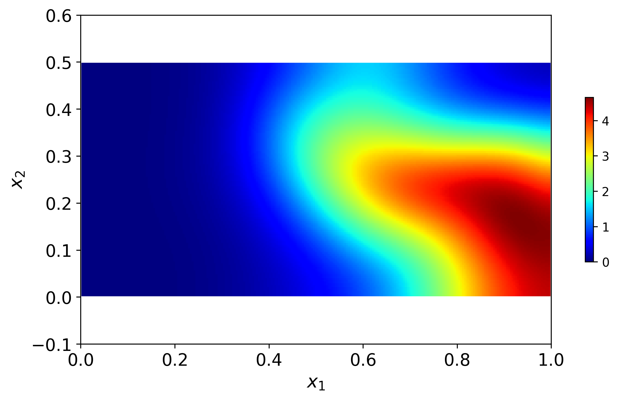
Refer to caption
Figure 8: Terminal condition for the backward ADE at the terminal time T=0.2𝑇0.2T=0.2.

We first test the same DNN architecture to approximate u~~𝑒\tilde{u} as in the forward ADE problem that has five hidden layers with 60 neurons per layer and an identity activation function in the last layer. Snapshots of the PINN solutions are shown in Figure 13. It can be seen that the solution develops negative concentration values and the magnitude of the negative values increases as time decreases.

In the source identification problems, the important quantities of interest are the trajectory of the center of mass, the initial source location, and the mass of the tracer as a function of time. The center of mass (X1c​(t),X2c​(t))superscriptsubscript𝑋1𝑐𝑑superscriptsubscript𝑋2𝑐𝑑(X_{1}^{c}(t),X_{2}^{c}(t)) of the plume can be found as:

X1c​(t)=∫0Lx2∫0Lx1x1​u^​(x1,x2,t)​𝑑x1​𝑑x2M​(t)X2c​(t)=∫0Lx2∫0Lx1x2​u^​(x1,x2,t)​𝑑x1​𝑑x2M​(t),superscriptsubscript𝑋1𝑐𝑑superscriptsubscript0subscript𝐿subscriptπ‘₯2superscriptsubscript0subscript𝐿subscriptπ‘₯1subscriptπ‘₯1^𝑒subscriptπ‘₯1subscriptπ‘₯2𝑑differential-dsubscriptπ‘₯1differential-dsubscriptπ‘₯2𝑀𝑑superscriptsubscript𝑋2𝑐𝑑superscriptsubscript0subscript𝐿subscriptπ‘₯2superscriptsubscript0subscript𝐿subscriptπ‘₯1subscriptπ‘₯2^𝑒subscriptπ‘₯1subscriptπ‘₯2𝑑differential-dsubscriptπ‘₯1differential-dsubscriptπ‘₯2𝑀𝑑\begin{split}X_{1}^{c}(t)=\frac{\int_{0}^{L_{x_{2}}}\int_{0}^{L_{x_{1}}}x_{1}\hat{u}(x_{1},x_{2},t)dx_{1}dx_{2}}{M(t)}\\ X_{2}^{c}(t)=\frac{\int_{0}^{L_{x_{2}}}\int_{0}^{L_{x_{1}}}x_{2}\hat{u}(x_{1},x_{2},t)dx_{1}dx_{2}}{M(t)},\\ \end{split} (52)

where M​(t)=∫0Lx2∫0Lx1u^​(x1,x2,t)​𝑑x1​𝑑x2𝑀𝑑superscriptsubscript0subscript𝐿subscriptπ‘₯2superscriptsubscript0subscript𝐿subscriptπ‘₯1^𝑒subscriptπ‘₯1subscriptπ‘₯2𝑑differential-dsubscriptπ‘₯1differential-dsubscriptπ‘₯2M(t)=\int_{0}^{L_{x_{2}}}\int_{0}^{L_{x_{1}}}\hat{u}(x_{1},x_{2},t)dx_{1}dx_{2} is the mass of the tracer time t𝑑t.

Figures 9(a) and (b) display the position of the center of mass and the tracer mass as functions of time computed from the PINN and reference solutions. It can be seen that the PINN solution incorrectly estimates the source location at time t=0𝑑0t=0 and the tracer mass. In the following section, we propose a modification to the DNN network structure to improve the accuracy of PINN for backward problems by enforcing the positivity of the PINN solution.

5.2 Modified DNN with a positive wrapper function in the last layer

To impose the positivity of the PINN solution, we add a positive β€œwrapper” function Οƒw​(z)subscriptπœŽπ‘€π‘§\sigma_{w}(z) to the output node of the u^^𝑒\hat{u} DNN. The output of the modified DNN thus becomes u^​(𝐱,t,Ξ³)=Οƒw​(ΟƒNh+1​(𝐱,t,Ξ³))^𝑒𝐱𝑑𝛾subscriptπœŽπ‘€subscript𝜎subscriptπ‘β„Ž1𝐱𝑑𝛾\hat{u}(\mathbf{x},t,\gamma)=\sigma_{w}(\sigma_{N_{h}+1}(\mathbf{x},t,\gamma)). The added wrapper function maps the output of the identity activation function ΟƒNh+1​(𝐱,t,Ξ³)subscript𝜎subscriptπ‘β„Ž1𝐱𝑑𝛾\sigma_{N_{h}+1}(\mathbf{x},t,\gamma) to u^∈[0,1]^𝑒01\hat{u}\in[0,1]. We use the sigmoid function as the wrapper function, Οƒw​(z)=11+eβˆ’zsubscriptπœŽπ‘€π‘§11superscript𝑒𝑧\sigma_{w}(z)=\frac{1}{1+e^{-z}}. Figure 14 shows snapshots of the PINN solution with the sigmoid wrapper function and the point errors. It can be seen that the PINN solution is strictly positive. Also, the maximum point errors in the PINN solution with the modified structure are smaller than in the PINN solution with the original DNN structure. For example, at time t=0.1, the maximum errors in the PINN solution with the modified and original DNNs are 0.3 and 0.7, respectively. The errors are largest at time t=0𝑑0t=0, with the maximum errors for the modified and original DNNs being 120 and 200, respectively. As expected, errors in the PINN solution of the backward ADE are largest at t=0𝑑0t=0.

Figure 9(a) compares the positions of the center of mass as functions of time obtained from the PINN solutions with the identity and sigmoid activation functions in the last layer as well as from the reference solution. The mass of the tracer, obtained from these solutions, is shown in Figure 9(b). Positions of the center of mass predicted with the sigmoid function are in significantly better agreement with the reference values than those predicted with the identity function. Also, the tracer mass in the PINN solution with the sigmoid wrapper function is in good agreement with the reference values, which is rather remarkable given that 30% of the total mass had left the domain before the terminal time T𝑇T.

We note that while we assume that the total mass M𝑀M at the time of release and the release time are known, this information is only used to normalize the solution so its maximum at all times is approximately 1. Therefore, any reasonable guess about the time of release and M𝑀M would produce similarly accurate predictions. We also note that there is no benefit of using the positive wrapper function for solving the forward ADE. We find that adding the wrapper function increases the error in the forward solution–for example, at late times the L2 error in the PINN solution for u𝑒u increases from 2% (without the wrapper function) to 8% (with the wrapper function). As stated in Section 2.2.1, the PINN method with the tanh activation functions (varying from -1 to 1) in the hidden layers has better convergence properties than that with positive activation functions such as a sigmoid function. Adding the sigmoid activation function in the last layer might have a similar effect on the convergence as having it in all hidden layers.

In the considered problem, the normalized solution is in the [0,1] range. Therefore, the sigmoid function can be used as a wrapper. If a normalized solution is of the order of one but can exceed one, then the softplus function s​o​f​t​p​l​u​s​(z)=l​o​g​(1+ez)π‘ π‘œπ‘“π‘‘π‘π‘™π‘’π‘ π‘§π‘™π‘œπ‘”1superscript𝑒𝑧softplus(z)=log(1+e^{z}) can be used as a wrapper instead of the sigmoid function. For the problem considered here, Figure 9 shows that the sigmoid and softplus wrapper functions give similar results.
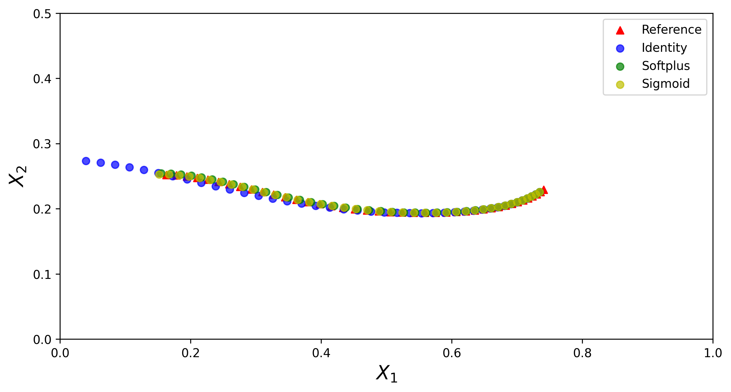
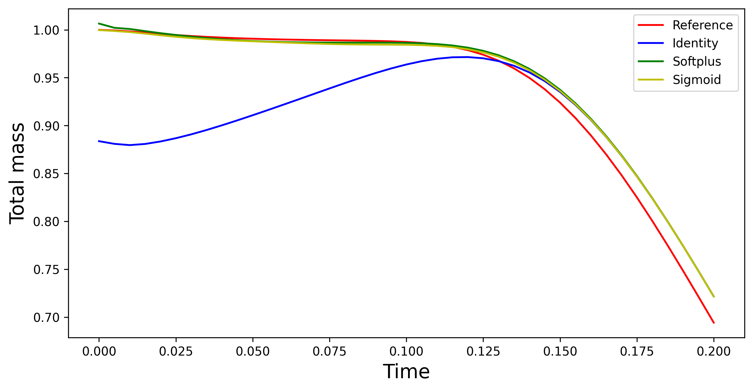
Refer to caption
(a)
Refer to caption
(b)
Figure 9: (a) The location of the center of mass obtained from the reference solution and PINN solution with three different activation functions in the output layer. (b) Total mass in the domain computed from the reference solution and the PINN solutions with different activation functions in the last layer. No measurements of u𝑒u are used to obtain the PINN solution u^^𝑒\hat{u}.

5.3 Data assimilation in the backward problem

In many source identification problems, the measurements of u𝑒u could be available at multiple times and not only at the terminal time. The measurements of u𝑒u can be included in the PINN formulation of the backward ADE solution in the same way as for the inverse ADE, i.e., by adding the L~d​a​t​asubscript~πΏπ‘‘π‘Žπ‘‘π‘Ž\tilde{L}_{data} (with Nk=Nh=0subscriptπ‘π‘˜subscriptπ‘β„Ž0N_{k}=N_{h}=0) in the loss function (50). We randomly select Nxsubscript𝑁π‘₯N_{x} locations where u𝑒u is sampled over time and assume that 100 measurements of u𝑒u over time are available at each of the Nxsubscript𝑁π‘₯N_{x} locations. Figure 10 shows the relative L2 error as a function of time for Nxsubscript𝑁π‘₯N_{x} ranging from 0 to 30. Our results show that at all times, the L2 error decreases with increasing Nxsubscript𝑁π‘₯N_{x}. At t=0𝑑0t=0 (when the errors are maximum), the errors are 30% and 8% for Nx=0subscript𝑁π‘₯0N_{x}=0 and 30, respectively. Snapshots of the backward PINN solution obtained with the measurements from 30 sensors (Nx=30subscript𝑁π‘₯30N_{x}=30) and the corresponding point errors are shown in Figure 15. The comparison with Figure 14, which depicts the solution obtained without u𝑒u measurements, demonstrates that u𝑒u measurements significantly improve solutions, especially at times close to 0 and near the (unknown) source location, with the maximum point errors decreasing from 1.2 to 0.2 at t=0.05𝑑0.05t=0.05 and from 120 to 60 at t=0𝑑0t=0.

Refer to caption
Figure 10: Relative L2subscript𝐿2L_{2} errors in the PINN solutions u^^𝑒\hat{u} versus time as functions of the number of u𝑒u measurements, Nxsubscript𝑁π‘₯N_{x}.

6 Conclusion

In this study, we presented the PINN method for parabolic PDEs with strongly perturbed initial conditions. We demonstrated that an accurate PINN solution can be obtained after a PDE is normalized such that the amplitude of the perturbation in the initial condition does not decay in time. Such normalization of the solution allows an accurate approximation of the solution with a relatively small DNN, which is a necessary condition for obtaining a convergent PINN solution. We also developed criteria for the weights in the loss function and an adaptive-in-time sampling of the PDE’s residuals that significantly improved the accuracy and efficiency of of the PINN method.

As an example of the parabolic PDE, we considered a time-dependent ADE with a Gaussian source initial condition and a non-uniform advection velocity field described by the Darcy flow equation with the heterogeneous hydraulic conductivity. For the forward ADE problem (known velocity field), we demonstrated that an accurate PINN solution of the normalized ADE can be obtained with a relatively small DNN size and the number of residual points as long as the residual points are placed adaptively in time. For the same DNN size and the number of residual points, the PINN solution of the original ADE was found to have large errors and non-physical negative values, regardless of how the residuals are sampled. Also, we found that there is a range of weight values that produce an accurate PINN solution of the normalized equation. The proposed criteria for weights resulted in the weights values within that range.

For the inverse ADE problem (unknown conductivity and the velocity field), we demonstrated that the proposed normalization, the criteria for weights, and adaptive residual sampling strategy produced accurate estimates of the ADE solution as well as estimates of the velocity and conductivity fields in combination with sparse measurements of the ADE solution and conductivity.

Finally, we demonstrated that the proposed methods allow for obtaining an accurate PINN solution of the backward ADE equation, including estimates of the center of mass and the mass of the tracer as functions of time within several percent of the reference values. With sparse measurements of the tracer concentration, the maximum L2 error in the backward solution (which occurs close to the location of the source and the time of release) was reduced from more than 30% to less than 9%.

7 Acknowledgments

This research was partially supported by the U.S. Department of Energy (DOE) Advanced Scientific Computing (ASCR) program. Pacific Northwest National Laboratory is operated by Battelle for the DOE under Contract DE-AC05-76RL01830.

References

  • [1] AndrewΒ R Barron. Approximation and estimation bounds for artificial neural networks. Machine learning, 14(1):115–133, 1994.
  • [2] AtilimΒ Gunes Baydin, BarakΒ A. Pearlmutter, AlexeyΒ Andreyevich Radul, and JeffreyΒ Mark Siskind. Automatic differentiation in machine learning: a survey. 2015.
  • [3] Shengze Cai, Zhiping Mao, Zhicheng Wang, Minglang Yin, and GeorgeΒ Em Karniadakis. Physics-informed neural networks (pinns) for fluid mechanics: A review. Acta Mechanica Sinica, pages 1–12, 2022.
  • [4] Salvatore Cuomo, VincenzoΒ Schiano diΒ Cola, Fabio Giampaolo, Gianluigi Rozza, Maziar Raissi, and Francesco Piccialli. Scientific machine learning through physics-informed neural networks: Where we are and what’s next, 2022.
  • [5] Xavier Glorot and Yoshua Bengio. Understanding the difficulty of training deep feedforward neural networks. In Proceedings of the thirteenth international conference on artificial intelligence and statistics, pages 249–256. JMLR Workshop and Conference Proceedings, 2010.
  • [6] Ian Goodfellow, Yoshua Bengio, and Aaron Courville. Deep learning. MIT press, 2016.
  • [7] ArlenΒ W Harbaugh. MODFLOW-2005, the US Geological Survey modular ground-water model: the ground-water flow process. US Department of the Interior, US Geological Survey Reston, VA, 2005.
  • [8] QiZhi He, David Barajas-Solano, Guzel Tartakovsky, and AlexandreΒ M Tartakovsky. Physics-informed neural networks for multiphysics data assimilation with application to subsurface transport. Advances in Water Resources, 141:103610, 2020.
  • [9] QiZhi He and AlexandreΒ M Tartakovsky. Physics-informed neural network method for forward and backward advection-dispersion equations. Water Resources Research, 57(7):e2020WR029479, 2021.
  • [10] Xiaotian Jiang, Danshi Wang, Qirui Fan, Min Zhang, Chao Lu, and Alan PakΒ Tao Lau. Solving the nonlinear schrΓΆdinger equation in optical fibers using physics-informed neural network. In Optical Fiber Communication Conference, pages M3H–8. Optica Publishing Group, 2021.
  • [11] GeorgeΒ Em Karniadakis, IoannisΒ G Kevrekidis, LuΒ Lu, Paris Perdikaris, Sifan Wang, and Liu Yang. Physics-informed machine learning. Nature Reviews Physics, 3(6):422–440, 2021.
  • [12] Daehyon Kim. Normalization methods for input and output vectors in backpropagation neural networks. International journal of computer mathematics, 71(2):161–171, 1999.
  • [13] DiederikΒ P. Kingma and Jimmy Ba. Adam: A method for stochastic optimization, 2017.
  • [14] Saiprasad Koturwar and Shabbir Merchant. Weight initialization of deep neural networks (dnns) using data statistics. arXiv preprint arXiv:1710.10570, 2017.
  • [15] YannΒ A LeCun, LΓ©on Bottou, GenevieveΒ B Orr, and Klaus-Robert MΓΌller. Efficient backprop. In Neural networks: Tricks of the trade, pages 9–48. Springer, 2012.
  • [16] DongΒ C Liu and Jorge Nocedal. On the limited memory bfgs method for large scale optimization. Mathematical programming, 45(1):503–528, 1989.
  • [17] Zhiping Mao, AmeyaΒ D Jagtap, and GeorgeΒ Em Karniadakis. Physics-informed neural networks for high-speed flows. Computer Methods in Applied Mechanics and Engineering, 360:112789, 2020.
  • [18] HΒ Nguyen and JΒ Reynen. A space-time least-square finite element scheme for advection-diffusion equations. Computer Methods in Applied Mechanics and Engineering, 42(3):331–342, 1984.
  • [19] Gadi Pinkas. Reasoning, nonmonotonicity and learning in connectionist networks that capture propositional knowledge. Artificial Intelligence, 77(2):203–247, 1995.
  • [20] Maziar Raissi, Paris Perdikaris, and GeorgeΒ E Karniadakis. Physics-informed neural networks: A deep learning framework for solving forward and inverse problems involving nonlinear partial differential equations. Journal of Computational Physics, 378:686–707, 2019.
  • [21] Yeonjong Shin, Jerome Darbon, and GeorgeΒ Em Karniadakis. On the convergence and generalization of physics informed neural networks. arXiv e-prints, pages arXiv–2004, 2020.
  • [22] AlexandreΒ M Tartakovsky, CΒ Ortiz Marrero, Paris Perdikaris, GuzelΒ D Tartakovsky, and David Barajas-Solano. Physics-informed deep neural networks for learning parameters and constitutive relationships in subsurface flow problems. Water Resources Research, 56(5):e2019WR026731, 2020.
  • [23] A.M. Tartakovsky, D.A. Barajas-Solano, and Q.Β He. Physics-informed machine learning with conditional karhunen-loΓ¨ve expansions. Journal of Computational Physics, 426:109904, 2021.
  • [24] Qingcan Wang etΒ al. Exponential convergence of the deep neural network approximation for analytic functions. arXiv preprint arXiv:1807.00297, 2018.
  • [25] Sifan Wang, Yujun Teng, and Paris Perdikaris. Understanding and mitigating gradient flow pathologies in physics-informed neural networks. SIAM Journal on Scientific Computing, 43(5):A3055–A3081, 2021.
  • [26] Yu-Hong Yeung, DavidΒ A. Barajas-Solano, and AlexandreΒ M. Tartakovsky. Physics-informed machine learning method for large-scale data assimilation problems. Water Resources Research, 58(5):e2021WR031023, 2022.
  • [27] Chunmiao Zheng, PΒ Patrick Wang, etΒ al. Mt3dms: a modular three-dimensional multispecies transport model for simulation of advection, dispersion, and chemical reactions of contaminants in groundwater systems; documentation and user’s guide. 1999.

Appendix A Figures of PINN simulation results and errors
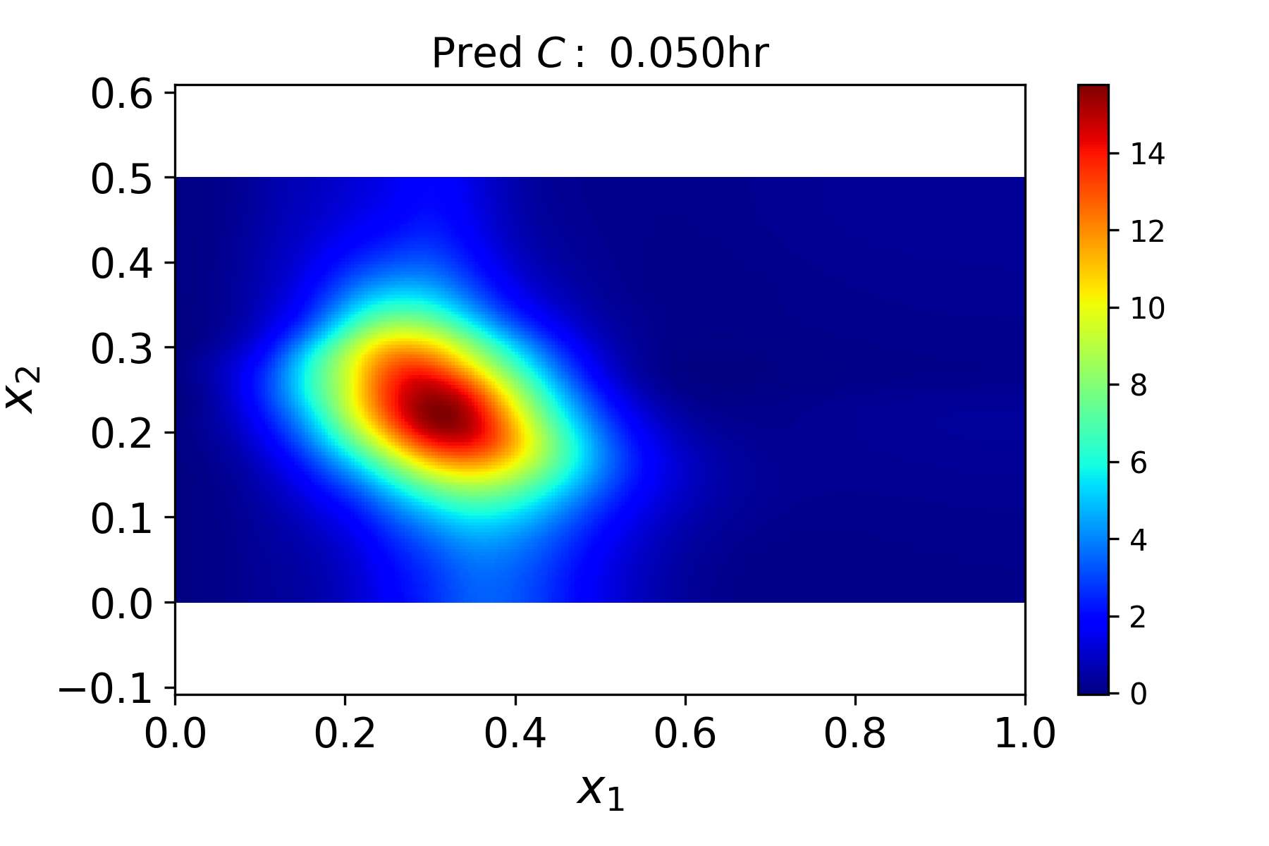
Refer to caption
Refer to caption
Refer to caption
Refer to caption
Refer to caption
Refer to caption
Refer to caption
Refer to caption
Refer to caption
Refer to caption
Refer to caption
Refer to caption
Figure 11: PINN solution u^^𝑒\hat{u} of the forward ADE (8) (left column), reference u𝑒u field (central column), and the absolute point errors u^βˆ’u^𝑒𝑒\hat{u}-u (right column) at times t=0.02𝑑0.02t=0.02, 0.1, 0.2, and 0.5. The weights are set to Ξ»i​c=Ξ»b​c​d=Ξ»b​c​n=10subscriptπœ†π‘–π‘subscriptπœ†π‘π‘π‘‘subscriptπœ†π‘π‘π‘›10\lambda_{ic}=\lambda_{bcd}=\lambda_{bcn}=10, Ξ»r​e​s=1subscriptπœ†π‘Ÿπ‘’π‘ 1\lambda_{res}=1. This PINN solution has the smallest L2 error among all considered weight combinations in Section 2.5.
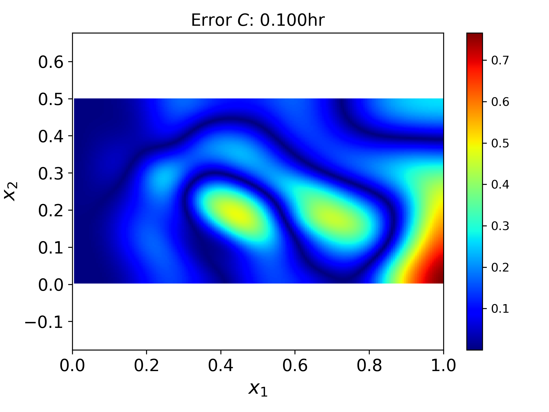
Refer to caption
Refer to caption
Refer to caption
Refer to caption
Refer to caption
Refer to caption
Refer to caption
Refer to caption
Refer to caption
Refer to caption
Refer to caption
Refer to caption
Figure 12: PINN solution u^^𝑒\hat{u} of the normalized forward ADE (8) (left column), reference normalized u~~𝑒\tilde{u} field (central column), and the absolute point errors u^βˆ’u~​u^𝑒~𝑒𝑒\hat{u}-\tilde{u}u (right column) at times t=0.02𝑑0.02t=0.02, 0.1, 0.2, and 0.5. The weights are set to Ξ»i​c=Ξ»b​c​d=126subscriptπœ†π‘–π‘subscriptπœ†π‘π‘π‘‘126\lambda_{ic}=\lambda_{bcd}=126, Ξ»b​c​n=Ξ»r​e​s=1subscriptπœ†π‘π‘π‘›subscriptπœ†π‘Ÿπ‘’π‘ 1\lambda_{bcn}=\lambda_{res}=1.
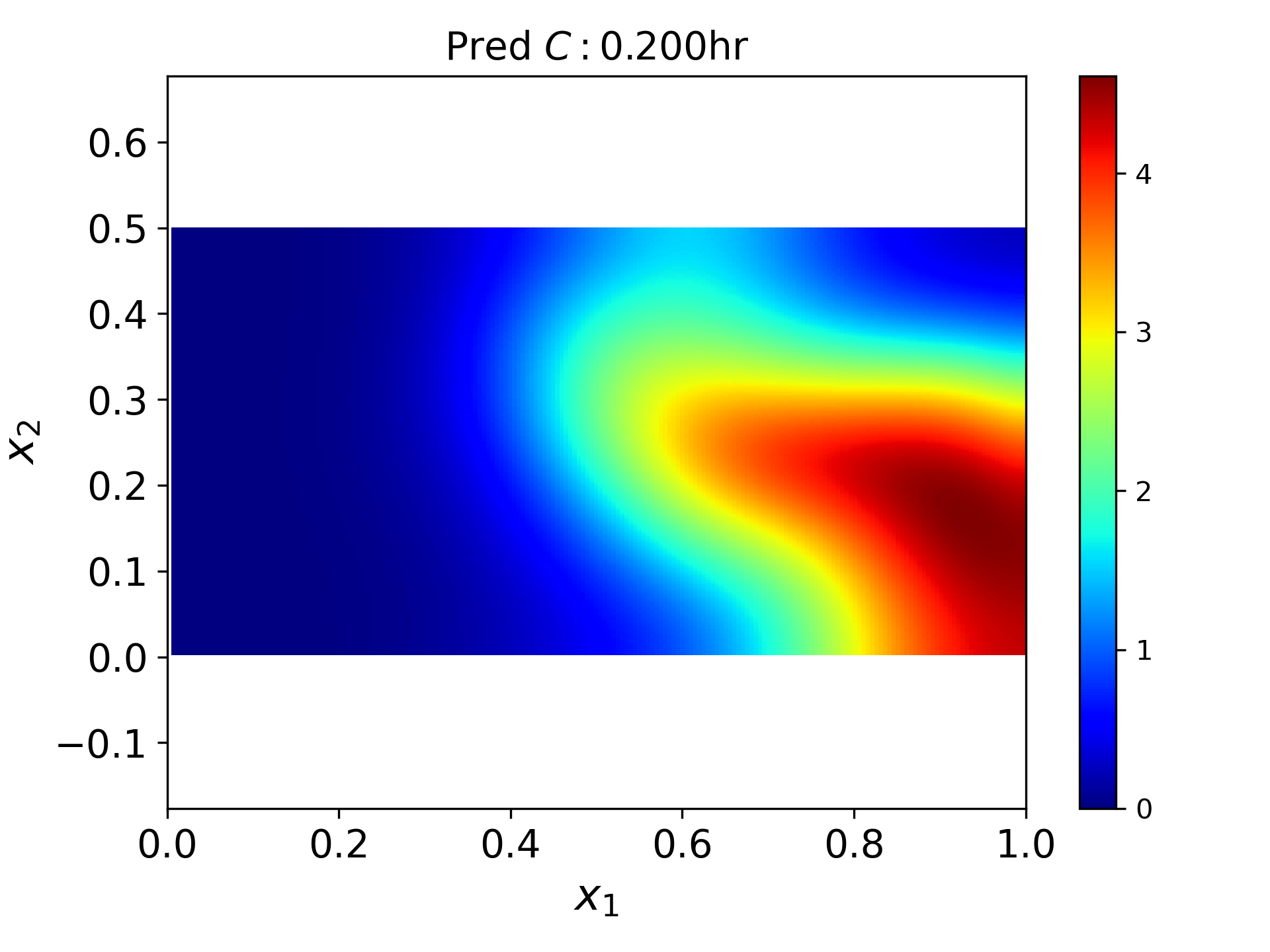
Refer to caption
Refer to caption
Refer to caption
Refer to caption
Refer to caption
Refer to caption
Refer to caption
Refer to caption
Refer to caption
Refer to caption
Refer to caption
Refer to caption
Figure 13: The backward PINN solution u^^𝑒\hat{u} (the first column), reference u𝑒u (the second column), and the absolute point error uβˆ’u^𝑒^𝑒u-\hat{u} (the third column) at t=0𝑑0t=0, 0.05, and 0.1, and at terminal time T=0.2𝑇0.2T=0.2. The identity activation function is used in the last layer. No measurements of u𝑒u are used to obtain the backward solution.
Refer to caption
Refer to caption
Refer to caption
Refer to caption
Refer to caption
Refer to caption
Refer to caption
Refer to caption
Refer to caption
Refer to caption
Refer to caption
Refer to caption
Figure 14: The backward PINN solution u^^𝑒\hat{u} (the first column), reference u𝑒u (the second column), and the absolute point error uβˆ’u^𝑒^𝑒u-\hat{u} (the third column) at t=0𝑑0t=0, 0.05, and 0.1, and at terminal time T=0.2𝑇0.2T=0.2. The sigmoid activation function is used in the last layer. No measurements of u𝑒u are used to obtain the backward solution.
Refer to caption
Refer to caption
Refer to caption
Refer to caption
Refer to caption
Refer to caption
Refer to caption
Refer to caption
Refer to caption
Refer to caption
Refer to caption
Refer to caption
Figure 15: The backward PINN solution u^^𝑒\hat{u} (the first column), reference u𝑒u (the second column), and the absolute point error uβˆ’u^𝑒^𝑒u-\hat{u} (the third column) at t=0𝑑0t=0, 0.05, and 0.1, and at terminal time T=0.2𝑇0.2T=0.2. The sigmoid activation function is used in the last layer. Nx=30subscript𝑁π‘₯30N_{x}=30 measurements of u𝑒u are used to obtain the PINN solution. Black dots denote the spatial locations of u𝑒u measurements.