Estimation and Specification Test for Diffusion Models with Stochastic Volatility

Abstract. Given the importance of continuous–time stochastic volatility models to describe the dynamics of interest rates, we propose a goodness–of–fit test for the parametric form of the drift and diffusion functions, based on a marked empirical process of the residuals. The test statistics are constructed using a continuous functional (Kolmogorov–Smirnov and Cramér–von Mises) over the empirical processes. In order to evaluate the proposed tests, we implement a simulation study, where a bootstrap method is considered for the calibration of the tests. As the estimation of diffusion models with stochastic volatility based on discretely sampled data has proven difficult, we address this issue by means of a Monte Carlo study for different estimation procedures. Finally, an application of the procedures to real data is provided.

Keywords. Diffusion processes; Goodness-of-fit; Stochastic differential equations; Stochastic volatility.

1 Introduction

Over the last five decades, continuous-time models have proven to be an essential part of the financial econometrics field. A large body of literature for the term structure of interest rates is written in continuous-time (Merton,, 1975) since the seminal works of Merton, (1973) and Black and Scholes, (1973). Different specifications have been proposed, such as the time-homogeneous diffusion given by a stochastic differential equation (SDE) driven by a Wiener process $W_{t}$,

$$\mathop{}\!\mathrm{d}r_{t}=m(r_{t},\boldsymbol{\theta})\mathop{}\!\mathrm{d}t+\nu(r_{t},\boldsymbol{\theta})\mathop{}\!\mathrm{d}W_{t},$$ (1)

defined on a complete probability space $\big{(}\Omega,\{\mathcal{F}_{t}\}_{t\in[0,T]},\mathbb{P}\big{)}$, where $\Omega$ is a nonempty set, $\mathcal{F}$ is a $\sigma$-algebra of subsets of $\Omega$ and $\mathbb{P}$ is a probability measure, $\mathbb{P}(\Omega)=1$. The process $r_{t}\in\mathbb{R}$ evolves over the interval $[0,T]$ in continuous time, according to the drift $m(\cdot)$ and diffusion $\nu(\cdot)$ functions. We work under a parametric framework, where $\boldsymbol{\theta}$ is an unknown parameter vector such that $\boldsymbol{\theta}\in\Theta\subset\mathbb{R}^{d}$ with $d$ a positive integer and $\Theta$ a compact set, and ${m(\cdot,\boldsymbol{\theta})\colon\mathbb{R}\times\Theta\rightarrow\mathbb{R}}$ and ${\nu(\cdot,\boldsymbol{\theta})\colon\mathbb{R}\times\Theta\rightarrow(0,\infty)}$.

In order to determine if the model is appropriated for a given time series, the parametric form of both drift and volatility functions can be tested. There exist several proposals for continuous-time model specification, such as Aït-Sahalia, (1996), Gao and King, (2004), Hong and Li, (2004), Chen et al., (2008), who used the marginal density function of the process; Dette and und Wilkau, (2003) and Dette et al., (2006), used a test statistic based on the $L^{2}$-distance between the diffusion function under the null hypothesis and the alternative; Arapis and Gao, (2006), Li, (2007), Gao and Casas, (2008) and Chen et al., (2019) proposals were based on smoothing techniques; Fan et al., (2001) and Fan and Zhang, (2003) developed a test based on a likelihood ratio test; Dette and Podolskij, (2008) and Podolskij and Ziggel, (2008) proposals were based on stochastic processes of the integrated volatility; and Monsalve-Cobis et al., (2011) and Chen et al., (2015) tests were based on empirical regression processes.

The empirical evidence obtained from the goodness-of-fit tests for the one-factor model in (1) proved unsatisfactory empirical fits and suggested that more flexible specifications for the volatility function were needed to capture the dynamics of returns of interest rates. Therefore, the literature has moved towards two-factor formulations, allowing the volatility function to incorporate a source of random variation, leading to a continuous-time stochastic volatility (SV) model, such as

$$\mathop{}\!\mathrm{d}r_{t} =m_{1}(r_{t},\boldsymbol{\theta})\mathop{}\!\mathrm{d}t+\sigma_{t}\nu_{1}(r_{t},\boldsymbol{\theta})\mathop{}\!\mathrm{d}W_{1,t},$$ (2)

$$\mathop{}\!\mathrm{d}g(\sigma_{t}) =m_{2}(g(\sigma_{t}),\boldsymbol{\theta})\mathop{}\!\mathrm{d}t+\nu_{2}(g(\sigma_{t}),\boldsymbol{\theta})\mathop{}\!\mathrm{d}W_{2,t},$$ (3)

where the functions $g,m_{1},\nu_{1},m_{2}$ and $\nu_{2}$ are sufficiently smooth and satisfy growth conditions to obtain existence and uniqueness for the stochastic differential equation solution, and $\boldsymbol{\theta}\in\Theta\subset\mathbb{R}^{d}$ is an unknown parameter vector. Several parametrizations of (2)–(3) have been examined, see Hull and White, (1987), Heston, (1993), Andersen and Lund, 1997a , Gallant and Tauchen, (1998), Eraker, (2001), or Christoffersen et al., (2009), among others.

Given the importance of the volatility in the financial market –a measure of risk that impacts in portfolio selection, option pricing, risk management or hedging–, its misspecification could lead to serious consequences. To overcome this, goodness-of-fit test should be used to study the adequacy of the proposed model towards the dynamics of the volatility. Some recent literature have addressed this issue, Lin et al., (2013, 2016) proposed a test based on the deviations between the empirical characteristic function and the parametric counterpart; Lin et al., (2014) considered a Bickel-Rosenblatt type test; Zu, (2015) used the $L^{2}$-distance to measure the discrepancy between the kernel and parametric deconvolution density estimator of an integrated volatility density; Vetter, (2015) test was based on a Kolmogorov-Smirnov statistic; Bull, (2017) proposed a wavelet-based test; Ebner et al., (2018) used Fourier methods; Christensen et al., (2019) proposal was based on the empirical distribution function; and Li et al., (2021) proposed a test for the integrated volatility of volatility.

In the present paper, we propose goodness-of-fit tests based on empirical processes, extending the methodology proposed by Monsalve-Cobis et al., (2011) to diffusion models with stochastic volatility, following the ideas suggested in González-Manteiga et al., (2017). Many goodness-of-fit test in the literature for continuous-time models, such as (2)–(3), focus on the stationary distribution of the volatility $\sigma_{t}^{2}$, however, we test that the diffusion and drift functions belong to a certain parametric family, that is,

$$\mathcal{H}_{0\nu} \colon\nu_{1}\in\{\nu_{1}(\cdot,\boldsymbol{\theta})\colon\boldsymbol{\theta}\in\Theta\},$$

$$\mathcal{H}_{0m} \colon m_{1}\in\{m_{1}(\cdot,\boldsymbol{\theta})\colon\boldsymbol{\theta}\in\Theta\},$$

respectively. To construct the test statistic we use integrated regression models, an approach discussed in Stute, (1997), where the study of a marked empirical process based on residuals was introduced and, subsequently, extended to time series in Koul and Stute, (1999). The empirical regression processes-based goodness-of-fit tests have been studied by other authors, see Diebolt, (1995) for a nonlinear parametric regression function or Diebolt and Zuber, (1999, 2001), for an extension to nonlinear and heteroscedastic regression.

Notwithstanding the importance of goodness-of-fit tools for continuous-time models, the latent factor in the stochastic volatility model challenges its implementation. In addition to the unobserved volatility, the process is specified in continuous-time but the observations occur at discrete time points. Therefore, the estimation problem should be addressed, as it hinders the goodness-of-fit procedures. We attempt to discuss the intricacies of different implementations, though a comprehensive survey of estimation methods for continuous-time unobserved state-variable models is beyond the scope of this paper. Several methods have been proposed for the estimation of stochastic volatility models (see Chen,, 2003, for a review). One of the earliest proposals was quasi-maximum likelihood, introduced in Harvey et al., (1994) (see, e.g., Ruiz,, 1994; Hurn et al.,, 2013). Another analytical methods include the Kalman, (1960) filter (see Broto and Ruiz,, 2004 for a survey on likelihood-based methods); the generalized method of moments (see, e.g., Melino and Turnbull,, 1990; Andersen and Sørensen,, 1996; Sapp,, 2009); approximate likelihood methods based on the characteristic function of the transition density (Bates,, 2006); closed-form moment-based procedure (Dufour and Valéry,, 2009); maximum likelihood using closed-form approximations and latent factor filtering (Aït-Sahalia et al.,, 2020). Simulation-based methods, though more computationally demanding, are increasingly used in the financial context. These methods include Markov Chain Monte Carlo techniques (see, e.g., Jacquier et al.,, 1994; Shephard and Pitt,, 1997; Kim et al.,, 1998; Eraker,, 2001; Chib et al.,, 2002; Johannes and Polson,, 2010; Kastner and Frühwirth-Schnatter,, 2014); particle filters (see, e.g., Kotecha and Djuric,, 2003; Carvalho et al.,, 2010; Lopes and Tsay,, 2011; Kantas et al.,, 2015); Expectation-Maximization algorithms (see, e.g., Dempster et al.,, 1977; Little and Rubin,, 2019); simulated maximum-likelihood (see, e.g., Danielsson and Richard,, 1993; Sandmann and Koopman,, 1998; Durham,, 2006); integrated nested Laplace approximations (INLA) methods (Rue et al.,, 2009).

The rest of the paper is structured as follows. Section 2 provides an outline of estimation methods and Monte Carlo experiments are designed in order to discuss the finite sample performance of the procedures. In Section 3, the goodness-of-fit tests for the drift and diffusion functions are introduced, while in Section 4 a simulation study of the proposed tests is implemented. Real data application to interest rate series is presented in Section 5 and conclusions are drawn in Section 6.

2 Estimation of diffusion models with latent variables

Given a two-factor continuous-time diffusion model as in (2)–(3), where the state $r_{t}$ is observable but the volatility $\sigma_{t}$ is a latent factor, although the model is formulated in continuous-time, data are sampled in discrete time points. Therefore, a discretized version of the diffusion equations should be consider to estimate the model parameters. Taking a popular specification, such as

$$\mathop{}\!\mathrm{d}r_{t} =(\alpha-\beta r_{t})\mathop{}\!\mathrm{d}t+\sigma_{t}\mathop{}\!\mathrm{d}W_{1,t},$$ (4)

$$\mathop{}\!\mathrm{d}\log\sigma_{t}^{2} =(\theta_{0}-\theta_{1}\log\sigma_{t}^{2})\mathop{}\!\mathrm{d}t+\xi\mathop{}\!\mathrm{d}W_{2,t},$$ (5)

where volatility follows an Ornstein-Uhlenbeck process (Stein and Stein,, 1991), we assume that the process $\{r_{t_{i}}\}_{i=0}^{n}$ is observed at equispaced discrete time points $0=t_{0}<t_{1}<\dots<t_{n}=T$ in the interval $[0,T=n\Delta]$, where the time step $\Delta$ between consecutive observations is fixed. The Euler-Maruyama (Maruyama,, 1955) method is commonly used as an approximation scheme, thereby, considering the SDE in (4)–(5), its discretized counterpart is given by

$$r_{t_{i}}-r_{t_{i-1}} =\alpha\Delta-\beta\Delta r_{t_{i-1}}+\sigma_{t_{i}}\sqrt{\Delta}\,\varepsilon_{1,t_{i}}, \varepsilon_{1,t_{i}}\sim N(0,1),$$ (6)

$$\log\sigma_{t_{i}}^{2}-\log\sigma_{t_{i-1}}^{2} =\theta_{0}\Delta-\theta_{1}\Delta\log\sigma_{t_{i-1}}^{2}+\xi\sqrt{\Delta}\,\varepsilon_{2,t_{i}}, \varepsilon_{2,t_{i}}\sim N(0,1),$$ (7)

with $i=0,1,\dots,n-1$, $t_{i}=i\Delta$, $r_{t_{0}}=r_{0}\in\mathbb{R}$, and where $\varepsilon_{1,t_{i}}$ and $\varepsilon_{2,t_{i}}$ are independent identically distributed (i.i.d.) standard Gaussian variables, given the independent and Gaussian increments property of the Wiener process.

In the remainder of this section, we give an outline of estimation methods procedures to estimate the unknown parameter vector. The state-space models allow an easily interpretable and flexible framework for stochastic volatility models, therefore, we focus on estimation procedures that are maximum likelihood-based on a state space model representation. We begin introducing a filtering algorithm and, as several Monte Carlo-based approximations for state-space models are available, we also consider this Bayesian approach, as well as sequential Monte Carlo methods or particle filters.

2.1 Kalman Filter

The dynamic linear model (Kalman,, 1960) considers that the observation vector $\boldsymbol{y}_{t}$ is generated by the state-space model

$$\boldsymbol{x}_{t} =\mathbf{\Phi}\boldsymbol{x}_{t-1}+\boldsymbol{w}_{t},\qquad \boldsymbol{w}_{t}\sim\text{iid}~{}N(0,\mathbf{Q}),$$ (8)

$$\boldsymbol{y}_{t} =\mathbf{A}_{t}\boldsymbol{x}_{t}+\boldsymbol{v}_{t},\qquad \;\boldsymbol{v}_{t}\sim\text{iid}~{}N(0,\mathbf{R}),$$ (9)

where $\boldsymbol{x}_{t}\in\mathbb{R}^{p}$ is the unknown state vector, $\boldsymbol{y}_{t}\in\mathbb{R}^{q}$ is the observed data vector, $\mathbf{A}_{t}\in\mathbb{R}^{q\times p}$ is the observation matrix, $\mathbf{\Phi}\in\mathbb{R}^{p\times p}$ is the transition matrix and we assume that $\left\{\boldsymbol{w}_{t}\right\}$ and $\left\{\boldsymbol{v}_{t}\right\}$ are uncorrelated. Equation (8) is known as the state equation and equation (9) as observation equation. The state vector $\boldsymbol{x}_{t}$ is latent, which provides an adequate framework for the stochastic volatility model. Let $\boldsymbol{x}_{t\mid{t-1}}=\mathbb{E}\left[\boldsymbol{x}_{t}\mid Y_{t-1}\right]$ and $\mathbf{P}_{t\mid{t-1}}=\mathbb{E}\left[(\boldsymbol{x}_{t}-\boldsymbol{x}_{t\mid{t-1}})(\boldsymbol{x}_{t}-\boldsymbol{x}_{t\mid{t-1}})^{\prime}\mid Y_{t-1}\right]$, with initial state $\boldsymbol{x}_{0}\sim N(\boldsymbol{x}_{0\mid 0},\mathbf{P}_{0\mid 0})$, given the data $Y_{s}=\{y_{1},\dots,y_{s}\}$ we have

$$\boldsymbol{x}_{t} \mid Y_{t-1} \sim N(\boldsymbol{x}_{t\mid{t-1}},\mathbf{P}_{t\mid{t-1}}),$$ (10)

$$\boldsymbol{y}_{t} \mid Y_{t-1} \sim N(\boldsymbol{y}_{t\mid{t-1}},\mathbf{\Sigma}_{t\mid{t-1}}),$$ (11)

$$\boldsymbol{x}_{t} \mid Y_{t} \sim N(\boldsymbol{x}_{t\mid t},\mathbf{P}_{t\mid t}),$$ (12)

which are the propagation, predictive and filtering density, respectively, with

$$\boldsymbol{x}_{t\mid{t-1}} =\mathbf{\Phi}\boldsymbol{x}_{{t-1}\mid{t-1}},\qquad \mathbf{P}_{t\mid{t-1}}=\mathbf{\Phi}\mathbf{P}_{{t-1}\mid{t-1}}\mathbf{\Phi}^{\prime}+\mathbf{Q},$$

$$\boldsymbol{y}_{t\mid{t-1}} =\mathbf{A}_{t}\boldsymbol{x}_{t\mid{t-1}},\qquad \mathbf{\Sigma}_{t}=\mathbf{A}_{t}\mathbf{P}_{t\mid{t-1}}\mathbf{A}_{t}^{\prime}+\mathbf{R},$$

$$\boldsymbol{x}_{t\mid t} =\boldsymbol{x}_{t\mid{t-1}}+\mathbf{K}_{t}\boldsymbol{\varepsilon}_{t},\qquad \mathbf{P}_{t\mid t}=\mathbf{P}_{t\mid{t-1}}-\mathbf{K}_{t}\mathbf{\Sigma}_{t}\mathbf{K}_{t}^{\prime},$$

where $\boldsymbol{\varepsilon}_{t}=\boldsymbol{y}_{t}-\mathbf{A}_{t}\boldsymbol{x}_{t\mid{t-1}}$ are the prediction errors and $\mathbf{K}_{t}=\mathbf{P}_{t\mid{t-1}}\mathbf{A}_{t}^{\prime}\mathbf{\Sigma}_{t}^{-1}$ is the Kalman gain. In state space models the aim is usually the estimation of the latent state vector $\boldsymbol{x}_{t}$ through filtering, for which we need to estimate the marginal distribution of the state vector given the observations, $p(\boldsymbol{x}_{t}\mid Y_{t})$. In Equations (10)–(12) linearity and the gaussianity of errors are assumed, but more general state space models can be considered. For this linear model, the Kalman Filter (Kalman,, 1960) can be used to estimate the distribution $p(\boldsymbol{x}_{t}\mid Y_{t})$ and computing the likelihood using the innovations. The discretized OU model in (6)–(7) is not linear so, in order to use the Kalman Filter with the state-space model (8)–(9), we first need to linearize it. Taking the residuals from the linear regression, $e_{t_{i}}=[r_{t_{i}}-\alpha\Delta+(1-\beta\Delta)r_{t_{i-1}}]/\sqrt{\Delta}=\sigma_{t_{i}}\varepsilon_{1,t_{i}}$, we define the logarithm of the squared residuals

$$y_{t_{i}}=\log e_{t_{i}}^{2}\quad\text{and}\quad h_{t_{i}}=\log\sigma_{t_{i}}^{2},$$

therefore, the model can be linearized as follows, parameterizing $\phi_{0}=\Delta\theta_{0}$, $\phi_{1}=(1-\theta_{1}\Delta)$,

$$y_{t_{i}} =h_{t_{i}}+v_{t_{i}},\qquad\quad v_{t_{i}}\sim\log\chi^{2}_{1},$$ (13)

$$h_{t_{i}} =\phi_{0}+\phi_{1}h_{t_{i-1}}+w_{t_{i}},\qquad\quad w_{t_{i}}\sim N(0,\sigma_{w}^{2}),$$ (14)

with $w_{t_{i}}=\xi\sqrt{\Delta}\,\varepsilon_{2,t_{i}}$ a Gaussian distributed variable, as $\varepsilon_{2,t_{i}}$ is an standard Gaussian variable, and where $\sigma_{w}^{2}=\Delta\xi^{2}$. The error term in the space equation (13) follows a log chi-squared with one degree of freedom, as $v_{t_{i}}=\log\varepsilon_{1,t_{i}}^{2}$ and $\varepsilon_{1,t_{i}}\sim N(0,1)$. The density of the $\log\chi^{2}_{1}$ is

$$f(x)=\frac{1}{\sqrt{2\pi}}\exp\bigg{(}-\frac{1}{2}\bigg{[}\exp(x)-x\bigg{]}\bigg{)},\qquad x\in\mathbb{R},$$

with mean $\mathbb{E}\left[v_{t_{i}}\right]=\psi(1)-\log 2\approx-1.2704$, where $\psi(\cdot)$ is a digamma function, and variance $\mathbb{V}\mathrm{ar}\left[v_{t_{i}}\right]=\pi^{2}/2\approx 4.9348$. As this density is skewed (see Figure 1), it departs from the Gaussian assumption, thus different approaches have been proposed in the literature. Shumway and Stoffer, (2000) proposed modeling the $\log\chi^{2}_{1}$ with a mixture of two Gaussian variables, one centered at zero, such as $\eta_{t_{i}}=I_{t_{i}}z_{0,t_{i}}+(1-I_{t_{i}})z_{1,t_{i}}$, where $z_{0,t_{i}}\sim N(0,\sigma_{0}^{2})$ and $z_{1,t_{i}}\sim N(\mu_{1},\sigma_{1}^{2})$ and $I_{t_{i}}$ is an i.i.d. Bernoulli process, $\mathbb{P}\left(I_{t_{i}}=0\right)=\pi_{0}$ and $\mathbb{P}\left(I_{t_{i}}=1\right)=\pi_{1}$, with $\pi_{0}+\pi_{1}=1$. Substituting the space equation (13) with

$$y_{t_{i}}=h_{t_{i}}+\eta_{t_{i}},$$ (15)

we have the filtering equations for this model:

$$h_{t_{i+1}\mid t_{i}} =\phi_{0}+\phi_{1}h_{t_{i}\mid t_{i-1}}+\sum_{j=0}^{1}\pi_{j,t_{i}}K_{j,t_{i}}\varepsilon_{j,t_{i}}$$ (16)

$$P_{t_{i+1}\mid t_{i}} =\phi_{1}^{2}P_{t_{i}\mid t_{i-1}}+\sigma_{w}^{2}-\sum_{j=0}^{1}\pi_{j,t_{i}}K_{j,t_{i}}^{2}\Sigma_{j,t_{i}}$$

$$\begin{split}\epsilon_{0,t_{i}}&=y_{t_{i}}-h_{t_{i}\mid t_{i-1}}\\ \Sigma_{0,t_{i}}&=P_{t_{i}\mid t_{i-1}}+\sigma_{0}^{2}\\ K_{0,t_{i}}&=\phi_{1}P_{t_{i}\mid t_{i-1}}/\thinspace\Sigma_{0,t_{i}}\end{split}\qquad\begin{split}\epsilon_{1,t_{i}}&=y_{t_{i}}-h_{t_{i}\mid t_{i-1}}-\mu_{1}\\ \Sigma_{1,t_{i}}&=P_{t_{i}\mid t_{i-1}}+\sigma_{1}^{2}\\ K_{1,t_{i}}&=\phi_{1}P_{t_{i}\mid t_{i-1}}/\thinspace\Sigma_{1,t_{i}}\end{split}$$ (17)

where, given the density of $y_{t_{i}}$ conditional to its past values $Y_{t_{1}}$, $f(t_{i}\mid t_{i-1})$,

$$\pi_{j,t_{i}}=\frac{\pi_{1,t_{i}}f_{1}(t_{i}\mid t_{i-1})}{\pi_{0,t_{i}}f_{0}(t_{i}\mid t_{i-1})+\pi_{1,t_{i}}f_{1}(t_{i}\mid t_{i-1})}\vspace{0.5\baselineskip}$$

and $f_{j}(t_{i}\mid t_{i-1})=N(x_{t_{i}\mid t_{i-1}}+\mu_{j},\Sigma_{j,t_{i}})$, for $j=0,1$ and $\mu_{0}=0$. The distribution $\pi_{j,t_{i}}$, for $j=0,1$, is specified a priori, usually uniform priors are chosen, $\pi_{0,t_{i}}=\pi_{1,t_{i}}=1/2$. Let $\boldsymbol{\theta}=(\phi_{0},\phi_{1},\sigma_{w}^{2},\mu_{1},\sigma_{0}^{2},\sigma_{1}^{2})^{\prime}$ be the vector of unknown parameters, maximum likelihood can be used for estimation, maximizing the log-likelihood $\ln\thinspace\mathcal{L}_{Y}(\boldsymbol{\theta})$ given by

$$\ln\thinspace\mathcal{L}_{Y}(\boldsymbol{\theta})=\sum_{i=1}^{n}\ln\left(\sum_{j=0}^{1}\pi_{j,t_{i}}N\Big{(}x_{t_{i}\mid t_{i-1}}+\mu_{j},\sigma_{j}^{2}\Big{)}\right),$$ (18)

Algorithms like the EM (Dempster et al.,, 1977) or the Newton-Raphson can be considered to maximize the log-likelihood in (18), as in Shumway and Stoffer, (1982) and Jones, (1980), for an example of both approaches.

2.2 Markov Chain Monte Carlo

Given the discrete version (13)–(14) of the SDE in (4)–(5), we have the popular parametrization of the discretized stochastic volatility model,

$$e_{t_{i}} =\exp\left(h_{t_{i}}/2\right)\epsilon_{t_{i}},\qquad \varepsilon_{t_{i}}\sim N(0,1),$$ (19)

$$h_{t_{i}} =\phi_{0}+\phi_{1}h_{t_{i-1}}+w_{t_{i}},\qquad w_{t_{i}}\sim N(0,\sigma_{w}^{2})$$ (20)

where $e_{t_{i}}$ are the residuals from the linear regression $r_{t_{i}}=\alpha\Delta+(1-\beta\Delta)r_{t_{i-1}}+e_{t_{i}}$, with $h_{t_{i}}=\log\sigma_{t_{i}}^{2}$, $\phi_{0}=\Delta\theta_{0}$, $\phi_{1}=(1-\theta_{1}\Delta)$ and $\sigma_{w}^{2}=\Delta\xi^{2}$. The model in (19) can be linearized by taking the logarithm of the squared observations, $y_{t_{i}}=\ln e_{t_{i}}^{2}$, as in (13). In the Bayesian approach of the estimation problem, the unknown parameter vector $\boldsymbol{\theta}=(\phi_{0},\phi_{1},\sigma_{w}^{2})^{\prime}$, with $\boldsymbol{\theta}\in\Theta\subset\mathbb{R}^{3}$, we consider a prior distribution of $\boldsymbol{\theta}$ over the parameter space $\Theta$. Given the prior distribution $\pi(\boldsymbol{\theta})$, we use Bayes’ Theorem to obtain the posterior distribution of the parameter vector,

$$p(\boldsymbol{\theta}\mid\boldsymbol{e})=\frac{p(\boldsymbol{e}\mid\boldsymbol{\theta})\pi(\boldsymbol{\theta})}{\int_{\Theta}p(\boldsymbol{e}\mid\boldsymbol{\theta})\pi(\boldsymbol{\theta})\mathop{}\!\mathrm{d}\boldsymbol{\theta}}\propto p(\boldsymbol{e}\mid\boldsymbol{\theta})\pi(\boldsymbol{\theta}),$$

where $\boldsymbol{e}=\{e_{t_{i}}\}_{i=0}^{n}$ is the vector of residuals. As a closed form solution might not exist, or its calculation is too difficult, sampling methods can be used to overcome this problem, such as Markov Chain Monte Carlo (MCMC) procedures, for example. Different MCMC procedures have been proposed to estimate the SV model (see Shephard,, 1993; Jacquier et al.,, 1994, for initial proposals), where the focus is targeted to the posterior density $p(\boldsymbol{\theta},\boldsymbol{h}\mid\boldsymbol{e})$, with $\boldsymbol{h}=\{h_{t_{i}}\}_{i=0}^{n}$, as the direct analysis of $p(\boldsymbol{\theta}\mid\boldsymbol{e})$ is not possible and the likelihood function $\mathcal{L}(\boldsymbol{e}\mid\boldsymbol{\theta})$ is intractable. Through Bayes’ Theorem we have that $p(\boldsymbol{h},\boldsymbol{\theta}\mid\boldsymbol{e})\propto p(\boldsymbol{e}\mid\boldsymbol{h})p(\boldsymbol{h}\mid\boldsymbol{\theta})p(\theta)$, and via MCMC methods we can sample from $p(\boldsymbol{\theta},\boldsymbol{h}\mid\boldsymbol{e})$. Using the Gibbs sampler we can produce samples from the posterior $p\big{(}h_{t_{i}}\mid\boldsymbol{h}_{-t_{i}},e_{t_{i}},\boldsymbol{\theta}\big{)}$, for $i=1,\dots,n$ where $\boldsymbol{h}_{-t_{i}}=(h_{t_{0}},\dots,h_{t_{i-1}},h_{t_{i+1}},\dots,h_{t_{n}})^{\prime}$, and $p\big{(}\boldsymbol{\theta}\mid\boldsymbol{e},\boldsymbol{h}\big{)}$, so that these samples will converge to those generated from $p\big{(}\boldsymbol{\theta},\boldsymbol{h}\mid\boldsymbol{e}\big{)}$. Let $\boldsymbol{h}_{t_{a:b}}=(h_{t_{a}},\dots,h_{t_{b}})^{\prime}$, the Gibbs sampler algorithm for the discrete model (19)–(20) is given in Algorithm 1.

Algorithm 1 (Gibbs sampling algorithm).

For $j=0,\dots,n$, the Gibbs sampler proceeds as follows, setting $j=0$:

1. Initialize $\boldsymbol{h}^{(0)}$ and $\boldsymbol{\theta}^{(0)}$.

2. Sample $\boldsymbol{h}^{(j+1)}$ from $p\big{(}\boldsymbol{h}\mid\boldsymbol{e},\boldsymbol{\theta}^{(j)}\big{)}$.

3. Sample $\boldsymbol{\theta}^{(j+1)}$ from $p\big{(}\boldsymbol{\theta}\mid\boldsymbol{e},\boldsymbol{h}^{(j+1)}\big{)}$.

   1. Sample $\sigma_{w}^{2}\mid\boldsymbol{e},\boldsymbol{h},\phi_{0},\phi_{1}$.

   2. Sample $\phi_{1}\mid\boldsymbol{h},\phi_{0},\sigma_{w}^{2}$.

   3. Sample $\phi_{0}\mid\boldsymbol{h},\phi_{1},\sigma_{w}^{2}$.

4. Set $j=j+1$ and go to $(2)$.

Step (2) in Algorithm 1 can be implemented by using a Metropolis-Hastings algorithm, where $p\big{(}\boldsymbol{h}\mid\boldsymbol{e},\boldsymbol{\theta}^{(j)}\big{)}$ is decomposed into conditionals, $p\big{(}h_{t_{i}}\mid\boldsymbol{h}_{-t_{i}}^{(j)},\boldsymbol{e},\boldsymbol{\theta}^{(j)}\big{)}$, for $i=1,\dots,n$, to sample $\boldsymbol{h}^{(j+1)}$. To sample $(h_{t_{0}}\mid\boldsymbol{\theta},\sigma_{w}^{2},h_{t_{1}})$, given $h_{t_{0}}\sim N(m_{0},c_{0})$ and $h_{t_{1}}\mid h_{t_{0}}\sim N(\phi_{0}+\phi_{1}h_{t_{0}},\sigma_{w}^{2})$, we can use Bayes’ theorem leading to

$$h_{t_{0}}\mid h_{t_{1}}\sim N(m_{1},c_{1}),$$

where $m_{1}=c_{1}\left[c_{0}^{-1}m_{0}+\phi_{1}\sigma_{w}^{-2}(h_{1}-\phi_{0})\right]$ and $c_{1}=(c_{0}^{-1}+\phi_{1}^{2}\sigma_{w}^{-2})^{-1}$. Regarding the conditional prior distribution of $h_{t_{i}}$, for $i=1,\dots,n-1$ we have

$$\begin{pmatrix}h_{t_{i}}\\ h_{t_{i+1}}\end{pmatrix}\sim N\left[\begin{pmatrix}\phi_{0}+\phi_{1}h_{t_{i-1}}\\ (1+\phi_{1})\phi_{0}+\phi_{1}^{2}h_{t_{i-1}}\end{pmatrix},\sigma_{w}^{2}\begin{pmatrix}1&\phi_{1}\\ \phi_{1}&1+\phi_{1}^{2}\end{pmatrix}\right],$$

therefore

$$(h_{t_{i}}\mid h_{t_{i-1}},h_{t_{i+1}},\boldsymbol{\theta},\sigma_{w}^{2}) ~{}\sim~{}N(\mu_{t_{i}},\nu^{2}),$$

$$(h_{t_{n}}\mid h_{t_{n-1}},\boldsymbol{\theta},\sigma_{w}^{2}) ~{}\sim~{}N(\mu_{t_{n}},\sigma_{w}^{2}),$$

where

$$\mathbb{E}\left[h_{t_{i}}\mid h_{t_{i-1}},h_{t_{i+1}},\boldsymbol{\theta},\sigma_{w}^{2}\right] =\mu_{t_{i}}=\left(\frac{1-\phi_{1}}{1+\phi_{1}^{2}}\right)\phi_{0}+\left(\frac{\phi_{1}}{1+\phi_{1}^{2}}\right)(h_{t_{i-1}}+h_{t_{i+1}}),$$

$$\mathbb{V}\textnormal{ar}\left[h_{t_{i}}\mid h_{t_{i-1}},h_{t_{i+1}},\boldsymbol{\theta},\sigma_{w}^{2}\right] =\nu^{2}=\sigma_{w}^{2}(1+\phi_{1}^{2})^{-1}$$

and

$$\mathbb{E}\left[h_{t_{n}}\mid h_{t_{n-1}},\boldsymbol{\theta},\sigma_{w}^{2}\right] =\mu_{t_{n}}=\phi_{0}+\phi_{1}h_{t_{n-1}}.$$

We can sample $h_{t_{i}}$ via independent Metropolis-Hastings, let $f_{N}(t_{i}\mid a,b)$ denote the Gaussian density distribution with mean $a$ and variance $b$, the full conditional distribution of $h_{t_{i}}$ is given by

$$p(h_{t_{i}}\mid\boldsymbol{h}_{-t_{i}},\boldsymbol{e},\boldsymbol{\theta},\sigma_{w}^{2})=p(h_{t_{i}}\mid h_{t_{i-1}},h_{t_{i+1}},\boldsymbol{\theta},\sigma_{w}^{2})\;p(\boldsymbol{e}\mid h_{t_{i}})=f_{N}(h_{t_{i}};\mu_{t},\nu^{2})\;f_{N}(e_{t_{i}};0,\exp(h_{t_{i}})).$$

Given that

$$\log p(e_{t_{i}}\mid h_{t_{i}})=\textnormal{const}-\frac{1}{2}h_{t_{i}}-\frac{e_{t_{i}}^{2}}{2}\exp(-h_{t_{i}})$$

and that a Taylor expansion of $\exp(-h_{t_{i}})$ around $\mu_{t_{i}}$ leads to

$$\log p(e_{t_{i}}\mid h_{t_{i}}) \approx\textnormal{const}-\frac{1}{2}h_{t_{i}}-\frac{e_{t_{i}}^{2}}{2}\Big{[}\exp(-\mu_{t_{i}})-(h_{t_{i}}-\mu_{t_{i}})\exp(-\mu_{t_{i}})\Big{]},$$

$$g(h_{t_{i}}) =\exp\Big{(}-\frac{1}{2}h_{t_{i}}\left[1-e_{t_{i}}^{2}\exp(-\mu_{t})\right]\Big{)},$$

by combining $f_{N}(h_{t_{i}};\mu_{t_{i}},\nu^{2})$ and $g(h_{t_{i}})$ we have the proposal distribution

$$p(h_{t_{i}}\mid h_{-{t_{i}}},\boldsymbol{e},\boldsymbol{\theta},\sigma_{w}^{2})\equiv N(h_{t_{i}};\tilde{\mu}_{t_{i}},\nu^{2}),$$

where $\tilde{\mu}_{t_{i}}=\mu_{t_{i}}+\frac{1}{2}\nu^{2}(e_{t_{i}}^{2}\exp(-\mu_{t_{i}})-1)$. Algorithm 2 provides the independent Metropolis-Hastings algorithm, where the acceptance probability is given in step (3).

Algorithm 2 (Metropolis-Hastings algorithm).

For $i=1,\dots,n$ and $j=0,\dots,l$, the independent Metropolis-Hastings algorithm proceeds as follows:

1. Current state $h_{t_{i}}^{(j)}$,

2. Sample $h_{t_{i}}^{*}$ from $N(\tilde{\mu}_{t_{i}},\nu^{2})$

3. Compute the acceptance probability

   $$\alpha=\min\Bigg{\{}1,\frac{f_{N}\big{(}h_{t_{i}}^{*};\mu_{t_{i}},\nu^{2}\big{)}\;f_{N}\big{(}e_{t_{i}};0,\exp(h_{t_{i}}^{*})\big{)}}{f_{N}\big{(}h_{t_{i}}^{(j)};\mu_{t_{i}},\nu^{2}\big{)}\;f_{N}\big{(}e_{t_{i}};0,\exp(h_{t_{i}}^{(j)})\big{)}}\;\frac{f_{N}\big{(}h_{t_{i}}^{(j)};\tilde{\mu}_{t_{i}},\nu^{2}\big{)}}{f_{N}\big{(}h_{t_{i}}^{*};\tilde{\mu}_{t_{i}},\nu^{2}\big{)}\phantom{\big{|}}}\Bigg{\}}$$

4. New state:
   

   $$h_{t_{i}}^{(j+1)}=\begin{cases}h_{t_{i}}^{*}\;&\textnormal{w.p.}\quad\alpha\\[4.52083pt] h_{t_{i}}^{(j)}\;&\textnormal{w.p.}\quad 1-\alpha\end{cases}$$

Regarding the sampling of the hyperparameters $\boldsymbol{\theta}=(\phi_{0},\phi_{1},\sigma_{w}^{2})^{\prime}$ –step (3) in Algorithm 1–, setting the initial log volatility $h_{t_{0}}\sim N(m_{0},c_{0})$ and $\boldsymbol{\phi}=(\phi_{0},\phi_{1})^{\prime}$, the prior distributions of $\boldsymbol{\phi}$ and $\sigma_{w}^{2}$ are

$$\boldsymbol{\phi}\mid\sigma_{w}^{2} ~{}\sim~{}N(\boldsymbol{\theta}^{(0)},\sigma_{w}^{2}\mathbf{V}_{0}),$$

$$\sigma_{w}^{2} ~{}\sim~{}IG\left(\frac{\nu_{0}}{2},\frac{\nu_{0}s_{0}^{2}}{2}\right),$$

respectively. Conditional on $\boldsymbol{h}_{t_{0:n}}$, the posterior distribution of $\boldsymbol{\phi}$ and $\sigma_{w}^{2}$ is

$$(\boldsymbol{\phi}\mid\sigma_{w}^{2},\boldsymbol{e},h_{t_{0:n}}) ~{}\sim~{}N(\boldsymbol{\phi}^{(1)},\sigma_{w}^{2}\mathbf{V}_{1}),$$

$$(\sigma_{w}^{2}\mid\boldsymbol{e},\boldsymbol{h}_{t_{0:n}}) ~{}\sim~{}IG\left(\frac{\nu_{1}}{2},\frac{\nu_{1}s_{1}^{2}}{2}\right),$$

given that $\nu_{1}=\nu_{0}+n$,

$$\mathbf{X}=\begin{pmatrix}1&h_{t_{0}}\\ \vdots&\vdots\\ 1&h_{t_{n-1}}\end{pmatrix}$$

and

$$\mathbf{V}_{1} =(\mathbf{V}_{0}^{-1}+\mathbf{X}^{\prime}\mathbf{X})^{-1},$$

$$\boldsymbol{\phi}^{(1)} =\mathbf{V}_{1}(\mathbf{V}_{0}^{-1}\boldsymbol{\phi}^{(0)}+\mathbf{X}^{\prime}\boldsymbol{h}_{t_{1:n}}),$$

$$\nu_{1}s_{1}^{2} =\nu_{0}s_{0}^{2}+(\boldsymbol{e}-\mathbf{X}\boldsymbol{\phi}^{(1)})^{\prime}(\boldsymbol{e}-\mathbf{X}\boldsymbol{\phi}^{(1)})+(\boldsymbol{\phi}^{(1)}-\boldsymbol{\phi}^{(0)})^{\prime}\mathbf{V}_{0}^{-1}(\boldsymbol{\phi}^{(1)}-\boldsymbol{\phi}^{(0)}).$$

2.3 Particle Filter

Particle filters incorporate the sequential estimation approach of the Kalman Filter algorithms and the flexibility for modeling of MCMC sampling algorithms. Replacing the Kalman Filter recursions in (10) and (12) by

$$p\big{(}\boldsymbol{x}_{t_{i}}\mid Y_{t_{i-1}}\big{)} =\int p\big{(}\boldsymbol{x}_{t_{i}}\mid\boldsymbol{x}_{t_{i-1}}\big{)}p\big{(}\boldsymbol{x}_{t_{i-1}}\mid Y_{t_{i-1}}\big{)}\mathop{}\!\mathrm{d}\boldsymbol{x}_{t_{i-1}},$$ (21)

$$p\big{(}\boldsymbol{x}_{t_{i}}\mid Y_{t_{i}}\big{)} =\frac{p\big{(}Y_{t_{i}}\mid\boldsymbol{x}_{t_{i}}\big{)}p\big{(}\boldsymbol{x}_{t_{i}}\mid Y_{t_{i-1}}\big{)}}{p\big{(}Y_{t_{i}}\mid Y_{t_{i-1}}\big{)}},$$ (22)

respectively, leads to a more general dynamic model, where assumptions like normality and linearity can be relaxed. However, both distributions in (21) and (22) are intractable and computationally costly. Particle filters algorithms approximate $p\big{(}\boldsymbol{x}_{t_{i}}\mid Y_{t_{i}}\big{)}$ by drawing a set of $l$ i.i.d. particles $\{\boldsymbol{x}_{t_{i}}^{(j)}\}_{j=1}^{l}$, starting with a set of i.i.d. particles $\{\boldsymbol{x}_{t_{i-1}}^{(j)}\}_{j=1}^{l}$ approximating $p\big{(}\boldsymbol{x}_{t_{i-1}}\mid Y_{t_{i-1}}\big{)}$. Since the early sequential Monte Carlo algorithm proposed by West, (1992), several filters have been proposed in the literature, like the Bootstrap filter or sequential importance sampling with resampling (SISR) by Gordon et al., (1993) and the auxiliary particle filter or auxiliary SIR (ASIR) proposed by Pitt and Shephard, (1999), among others. Liu and West, (2001) proposed a filter for sequential learning, a variant of the auxiliary particle filtering (APF) algorithm, that combines the APF together with a kernel approximation to $p(\boldsymbol{\theta}\mid Y_{t_{i-1}})$ using a mixture of multivariate Gaussian distributions and shrinkage parameter to provide artificial evolution for the parameter vector $\boldsymbol{\theta}$. Therefore, the posterior distribution for $\boldsymbol{\theta}$ is approximated by the normal mixture

$$p\big{(}\boldsymbol{\theta}\mid Y_{t_{i}}\big{)}=\sum_{j=1}^{l}N\big{(}m^{(j)},h^{2}V_{t_{i}}\big{)},$$

where $m^{(j)}=a\boldsymbol{\theta}_{t_{i}}^{(j)}+(1-a)\tilde{\boldsymbol{\theta}}_{t_{i}}$, $a=\sqrt{1-h^{2}}$, $\tilde{\boldsymbol{\theta}}_{t_{i}}=\sum_{j=1}^{l}\boldsymbol{\theta}_{t_{i}}^{(j)}/l$ and $V_{t_{i}}=\sum_{j=1}^{l}(\boldsymbol{\theta}_{t_{i}}^{(j)}-\tilde{\boldsymbol{\theta}}_{t_{i}})(\boldsymbol{\theta}_{t_{i}}^{(j)}-\tilde{\boldsymbol{\theta}}_{t_{i}})^{\prime}/l$. The constant $a$ measures the extent of the shrinkage and $h$ controls the degree of overdispersion of the mixture (the choice of both parameters is discussed in Liu and West,, 2001). The general algorithm is displayed in Algorithm 3.

Algorithm 3 (Liu and West filter).

For $i=1,\dots,n$, a general Liu and West, (2001) filter algorithm runs as follows:

1. Set the prior point estimates $\{(\hat{\mu}_{t_{i+1}},m_{t_{i}})^{(j)}\}_{j=1}^{l}$ of $(x_{t_{i}},\boldsymbol{\theta})$ where $\hat{\mu}_{t_{i}}^{(j)}=\mathbb{E}\left[x_{t_{i+1}}\mid x_{t_{i}}^{(j)},\boldsymbol{\theta}^{(j)}\right]$.

2. Resample $\{(\tilde{x}_{t_{i}},\tilde{\boldsymbol{\theta}}_{t_{i}})^{(j)}\}_{j=1}^{l}$ from $\{(x_{t_{i}},\boldsymbol{\theta}_{t_{i}})^{(j)}\}_{j=1}^{l}$ with weights

   $$w_{t_{i+1}}^{(j)}\propto p\big{(}y_{t_{i+1}}\mid\hat{\mu}_{t_{i+1}}^{(j)},m^{(j)}\big{)}.$$

3. Propagate

   1. $\{\tilde{\boldsymbol{\theta}}_{t_{i}}^{(j)}\}_{j=1}^{l}$ via $N\big{(}\tilde{m}^{(j)},h^{2}V_{t_{i}}\big{)}$,

   2. $\{\tilde{x}_{t_{i}}^{(j)}\}_{j=1}^{l}$ via $p\big{(}x_{t_{i+1}}\mid\tilde{x}_{t_{i}}^{(j)},\tilde{\boldsymbol{\theta}}_{t_{i+1}}^{(j)}\big{)}$.

4. Resample $\{\big{(}x_{t_{i+1}},\boldsymbol{\theta}_{t_{i+1}}\big{)}^{(j)}\}_{j=1}^{l}$ from $\{\big{(}\tilde{x}_{t_{i+1}},\tilde{\boldsymbol{\theta}}_{t_{i+1}}^{(j)}\big{)}^{(j)}\}_{j=1}^{l}$ with weights

   $$w_{t_{i+1}}^{(j)}\propto\frac{p\big{(}y_{t_{i+1}}\mid\tilde{x}_{t_{i+1}}^{(j)},\tilde{\boldsymbol{\theta}}_{t_{i+1}}^{(j)}\big{)}}{p\big{(}y_{t_{i+1}}\mid\hat{\mu}_{t_{i+1}}^{(j)},\tilde{m}^{(j)}\big{)}}.$$

2.4 Comparative study

This section compares the results of the different estimation procedures applied to three parametrizations of the continuous-time two-factor model with stochastic volatility: we consider a simpler model, such as (4)–(5), which does not include a level parameter; a model with a more intricate volatility function, with level parameter, with and without correlated errors. We compare the parameter estimates obtained with the different procedures under Monte Carlo settings to examine their finite sample performance. Through all the models and procedures considered, we first estimate the parameters of the drift function $m_{1}(\cdot)$ in (2) and, subsequently, the residuals obtained are used in the procedures to estimate the parameter vector $\boldsymbol{\theta}$.

2.4.1 Ornstein-Uhlenbeck with stochastic volatility

Considering the Ornstein-Uhlenbeck model with stochastic volatility introduced in (4)–(5) and its discretized counterpart, (6)–(7), we have the discrete two-factor model

$$r_{t_{i+1}}-r_{t_{i}} =(\alpha-\beta r_{t_{i}})\Delta+\sigma_{t_{i}}\sqrt{\Delta}\varepsilon_{1,t_{i}},\qquad \varepsilon_{1,t_{i}}\sim N(0,1),$$

$$\log\sigma_{t_{i+1}}^{2} =\phi_{0}-\phi_{1}\log\sigma_{t_{i}}^{2}+w_{t_{i}},\qquad w_{t_{i}}\sim N(0,\sigma_{w}^{2}),$$

where $\phi_{0}=\theta_{0}\Delta$, $\phi_{1}=1-\theta_{1}\Delta$ and $\sigma_{w}^{2}=\Delta\xi^{2}$, with $i=0,1,\dots,n-1$ and initial condition $r_{t_{0}}=r_{0}\in\mathbb{R}$. To estimate the vector of parameters $\boldsymbol{\theta}=(\alpha,\beta,\phi_{0},\phi_{1},\sigma_{w}^{2})^{\prime}$ we first obtain the residuals from the linear regression $u_{t_{i}}=\alpha-\beta r_{t_{i}}+e_{t_{i}}$, where $u_{t_{i}}=(r_{t_{i+1}}-r_{t_{i}})/\Delta$. Therefore, in this first step we obtain the estimates of $\alpha$ and $\beta$ and thereafter we use the procedures to estimate the rest of the parameters using the residuals of the linear regression, $e_{t_{i}}=\sigma_{t_{i}}\Delta^{-1/2}\varepsilon_{1,t_{i}}$. The vector of parameter values considered for data simulation is $\boldsymbol{\theta}=(\alpha,\beta,\phi_{0},\phi_{1},\sigma_{w}^{2})^{\prime}=(0.01,0.3,-0.006,0.99,0.0225)^{\prime}$, with weekly frequency $(\Delta=1/52)$ for sample size $n\in\{520,1040,2080\}$, which corresponds to $T=10,20\text{ and }40$ years, respectively. A thousand realizations of random sample paths $\{r_{i\Delta}\}_{i=1}^{n}$ were generated, where the first $1000$ observations were discarded to remove the dependence on the initial value.

Tables 1–3 report the estimates for the three procedures considered: Markov Chain Monte Carlo (MCMC) method, using a Metropolis-Hastings algorithm within the Gibbs sampling; the Liu and West, (2001) filter (Particle Filter); and the Kalman, (1960) Filter. Tables include the mean and variance (Var) for one thousand simulations, along with the mean squared error (MSE). The estimates of the drift parameters $\alpha$ and $\beta$ were not obtained with the procedures, as mentioned, but rather fitting a linear regression. The simulation-based techniques show low MSE with the different sample sizes considered, while the Kalman Filter, thought for the smallest sample size $n$ has higher bias and variance, it particularly decreases when the observation window $T$ is extended, achieving a MSE closer to the other methods. Whilst the MCMC and the particle filter procedures do deliver accurate estimations, their computationally demanding nature and the practical implementation, highly model-dependent, are major disadvantages. On the other hand, the flexibility of the Kalman Filter can provide a good trade-off between speed and efficiency.

Parameter	True	Mean	Var	MSE
$\alpha$	$0.01$	$0.0195$	$0.6764$	$0.6765$
$\beta$	$0.3$	$0.8888$	$0.3903$	$0.7370$
MCMC
$\phi_{0}$	$-0.006$	$-0.0139$	$0.0019$	$0.0020$
$\phi_{1}$	$0.99$	$0.9692$	$0.0065$	$0.0069$
$\sigma_{w}^{2}$	$0.0225$	$0.0231$	$4.457\times 10^{-5}$	$4.490\times 10^{-5}$
Particle Filter
$\phi_{0}$	$-0.006$	$-0.0224$	$0.0011$	$0.0013$
$\phi_{1}$	$0.99$	$0.9370$	$0.0004$	$0.0032$
$\sigma_{w}^{2}$	$0.0225$	$0.0376$	$1.394\times 10^{-4}$	$3.663\times 10^{-4}$
Kalman Filter
$\phi_{0}$	$-0.006$	$-0.0420$	$0.0506$	$0.0519$
$\phi_{1}$	$0.99$	$0.9457$	$0.0467$	$0.0487$
$\sigma_{w}^{2}$	$0.0225$	$0.0410$	$9.213\times 10^{-4}$	$1.265\times 10^{-3}$

Table 1: Parameter estimates for the Ornstein-Uhlenbeck process with stochastic volatility, with sample size $n=520$ which corresponds to ten years ($T=10$) of weekly data ($\Delta=1/52$).

Parameter	True	Mean	Var	MSE
$\alpha$	$0.01$	$0.0089$	$0.1617$	$0.1617$
$\beta$	$0.3$	$0.5676$	$0.1240$	$0.1956$
MCMC
$\phi_{0}$	$-0.006$	$-0.0083$	$7.270\times 10^{-5}$	$7.781\times 10^{-5}$
$\phi_{1}$	$0.99$	$0.9851$	$6.075\times 10^{-5}$	$8.525\times 10^{-5}$
$\sigma_{w}^{2}$	$0.0225$	$0.0227$	$3.341\times 10^{-5}$	$3.345\times 10^{-5}$
Particle Filter
$\phi_{0}$	$-0.006$	$-0.0211$	$6.144\times 10^{-4}$	$8.422\times 10^{-4}$
$\phi_{1}$	$0.99$	$0.9501$	$2.597\times 10^{-4}$	$1.854\times 10^{-3}$
$\sigma_{w}^{2}$	$0.0225$	$0.0369$	$1.462\times 10^{-4}$	$3.539\times 10^{-4}$
Kalman Filter
$\phi_{0}$	$-0.006$	$-0.0168$	$3.885\times 10^{-3}$	$5.178\times 10^{-3}$
$\phi_{1}$	$0.99$	$0.9585$	$3.985\times 10^{-2}$	$4.181\times 10^{-2}$
$\sigma_{w}^{2}$	$0.0225$	$0.0350$	$1.902\times 10^{-4}$	$5.336\times 10^{-4}$

Table 2: Parameter estimates for the Ornstein-Uhlenbeck process with stochastic volatility, with sample size $n=1040$ which corresponds to ten years ($T=20$) of weekly data ($\Delta=1/52$).

Parameter	True	Mean	Var	MSE
$\alpha$	$0.01$	$0.0192$	$0.0508$	$0.0509$
$\beta$	$0.3$	$0.4378$	$0.0433$	$0.0623$
MCMC
$\phi_{0}$	$-0.006$	$-0.0071$	$2.699\times 10^{-5}$	$2.825\times 10^{-5}$
$\phi_{1}$	$0.99$	$0.9878$	$2.121\times 10^{-5}$	$2.585\times 10^{-5}$
$\sigma_{w}^{2}$	$0.0225$	$0.0226$	$2.323\times 10^{-5}$	$2.325\times 10^{-5}$
Particle Filter
$\phi_{0}$	$-0.006$	$-0.0176$	$3.167\times 10^{-4}$	$4.508\times 10^{-4}$
$\phi_{1}$	$0.99$	$0.9629$	$1.610\times 10^{-4}$	$8.958\times 10^{-4}$
$\sigma_{w}^{2}$	$0.0225$	$0.0344$	$1.420\times 10^{-4}$	$2.827\times 10^{-4}$
Kalman Filter
$\phi_{0}$	$-0.006$	$-0.0087$	$3.638\times 10^{-5}$	$1.329\times 10^{-3}$
$\phi_{1}$	$0.99$	$0.9874$	$2.627\times 10^{-5}$	$1.992\times 10^{-3}$
$\sigma_{w}^{2}$	$0.0225$	$0.0340$	$7.659\times 10^{-5}$	$4.200\times 10^{-4}$

Table 3: Parameter estimates for the Ornstein-Uhlenbeck process with stochastic volatility, with sample size $n=2080$ which corresponds to ten years ($T=40$) of weekly data ($\Delta=1/52$).

2.4.2 CKLS with stochastic volatility

In this section, a more intricate model is considered, based on the CKLS model proposed in Chan et al., (1992), where stochastic volatility is incorporated to the diffusion function. The CKLS model with stochastic volatility described by the Ornstein-Uhlenbeck (OU) process is given by

$$\mathop{}\!\mathrm{d}r_{t} =(\alpha-\beta r_{t})\mathop{}\!\mathrm{d}t+\sigma_{t}r_{t}^{\gamma}\mathop{}\!\mathrm{d}W_{1,t},$$ (23)

$$\mathop{}\!\mathrm{d}\log\sigma_{t}^{2} =(\theta_{0}-\theta_{1}\log\sigma_{t}^{2})+\xi\mathop{}\!\mathrm{d}W_{2,t},$$

and its discretized counterpart,

$$r_{t_{i+1}}-r_{t_{i}} =(\alpha-\beta r_{t})\Delta+\sigma_{t}r_{t_{i}}^{\gamma}\,(W_{1,t_{i+1}}-W_{1,t_{i}}),$$ (24)

$$\log\sigma_{t_{i+1}}^{2} =\phi_{0}-\phi_{1}\log\sigma_{t_{i}}^{2}+\xi\,(W_{2,t_{i+1}}-W_{2,t_{i}}),$$

where $\phi_{0}=\theta_{0}\Delta$ and $\phi_{1}=1-\theta_{1}\Delta$. This process has been proposed in the literature to model the short term interest rate (see Andersen and Lund, 1997a, ; ; among others), as it represents an extension of the classical stochastic volatility model to a continuous-time setting incorporating level effect, implying that volatility depends on the level of the interest rate and inducing conditional heteroskedasticity.

The Kalman Filter can be easily extended to allow modifications of the two-factor model. As indicated in Section 2.1, the error term in the space equation (13) follows a log chi-squared with one degree of freedom, and this has motivated different approaches in the literature. Shumway and Stoffer, (2000) modeled the $\log\chi^{2}_{1}$ with a mixture of two Gaussian variables (see the filtering equations (16)–(17)), while Kim et al., (1998) proposed a seven-component Gaussian mixture (see Chib et al.,, 2002, and Artigas and Tsay,, 2004), with weights $\pi_{i}$ and mean and variance ($N(\mu_{i},\sigma_{i}^{2})$ for $i\in\{1,\dots,7\}$) given in Table 4. A comparison of the true $\log\chi^{2}_{1}$ distribution with a Gaussian distribution and the two and seven Gaussian mixture is illustrated in Figure 1.

Component $i$	$1$	$2$	$3$	$4$	$5$	$6$	$7$
$\pi_{i}$	$0.00730$	$0.10556$	$0.00002$	$0.04395$	$0.34001$	$0.24566$	$0.25750$
$\mu_{i}$	$-11.400$	$-5.2432$	$-9.8373$	$1.5075$	$-0.6510$	$0.5248$	$-2.3586$
$\sigma^{2}_{i}$	$5.7960$	$2.6137$	$5.1795$	$0.1674$	$0.6401$	$0.3402$	$1.2626$

Table 4: Components of a mixture of seven Gaussian distributions, $N(\mu_{i},\sigma_{i}^{2})$, with weights $\pi_{i}$.

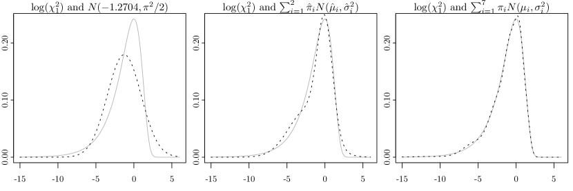
Figure 1: Comparison of the $\log\chi^{2}_{1}$ density function (solid line) and Gaussian density (left), mixture of two normal distributions (middle) and mixture of seven normal distributions (right).

A simulation study was conducted to compare both approaches. A thousand realizations of random sample paths for the CKLS-OU model in (23) were generated with weekly frequency, with $\boldsymbol{\theta}=(\alpha,\beta,\gamma,\phi_{0},\phi_{1},\xi)^{\prime}=(0.04,0.6,1.5,-0.013,0.998,0.4)^{\prime}$. Note that in the two mixture approach we estimate the parameter vector $\boldsymbol{\theta}$ and the components of the mixture –namely, $(\mu_{1},\sigma_{0}^{2},\sigma_{1}^{2})^{\prime}$, as $\mu_{0}=0$–, while in the seven mixture approach the means and variances of the Gaussian distributions remain fixed according to the values in Table 4.

The parameter estimates are summarized in Tables 5–7, for the two (Kalman Filter 2) and seven (Kalman Filter 7) mixture and three sample sizes $n\in\{520,1040,2080\}$. Though both methods provide a close performance, for small sample size (Table 5) the seven mixture filter provides lower mean squared error. However, larger sample sizes (Table 7) show an improvement for the two mixture filter, where the estimation of the parameter $\xi$, known as the volatility of volatility and hard to estimate accurately, outperforms the seven mixture filter. As an example, Figure 2 shows the estimated path (dotted) of the log volatility ($\log\sigma_{t}^{2}$) using the two and seven mixture approach, and a $95\%$ confidence interval for the estimated paths (shaded).

		Kalman Filter (2)				Kalman Filter (7)
	True	Mean	Var	MSE		Mean	Var	MSE
$\alpha$	$0.04$	$0.0731$	$0.0017$	$0.0028$		$0.0731$	$0.0017$	$0.0028$
$\beta$	$0.6$	$1.0964$	$0.3760$	$0.6224$		$1.0964$	$0.3760$	$0.6224$
$\gamma$	$1.5$	$1.5305$	$0.0243$	$0.0253$		$1.5009$	$0.0133$	$0.0133$
$\phi_{0}$	$-0.013$	$-0.4977$	$1.5604$	$1.7948$		$-0.2974$	$0.8113$	$0.8919$
$\phi_{1}$	$0.998$	$0.9249$	$0.0333$	$0.0386$		$0.9555$	$0.0190$	$0.0208$
$\xi$	$0.4$	$0.7284$	$1.1962$	$1.3040$		$0.6963$	$0.2206$	$0.3083$

Table 5: Parameter estimates for the discretized version of (23), as in (24), for the Kalman Filter algorithm with a mixture of two (left) and seven (right) Gaussian distributions. A thousand simulations were carried out with weekly data and $n=520$, which corresponds to $T=10$ years.

		Kalman Filter (2)				Kalman Filter (7)
	True	Mean	Var	MSE		Mean	Var	MSE
$\alpha$	$0.04$	$0.0567$	$0.0006$	$0.0008$		$0.0567$	$0.0006$	$0.0008$
$\beta$	$0.6$	$0.8508$	$0.1258$	$0.1887$		$0.8508$	$0.1258$	$0.1887$
$\gamma$	$1.5$	$1.5248$	$0.0072$	$0.0078$		$1.4983$	$0.0069$	$0.0069$
$\phi_{0}$	$-0.013$	$-0.1228$	$0.0996$	$0.1116$		$-0.0753$	$0.0299$	$0.0337$
$\phi_{1}$	$0.998$	$0.9825$	$0.0018$	$0.0021$		$0.9892$	$0.0006$	$0.0006$
$\xi$	$0.4$	$0.5865$	$0.0940$	$0.1288$		$0.6672$	$0.0507$	$0.1221$

Table 6: Simulation for weekly data and $n=1040$ ($T=20$ years).

		Kalman Filter (2)				Kalman Filter (7)
	True	Mean	Var	MSE		Mean	Var	MSE
$\alpha$	$0.04$	$0.0485$	$0.0002$	$0.0003$		$0.0485$	$0.0002$	$0.0003$
$\beta$	$0.6$	$0.7281$	$0.0509$	$0.0673$		$0.7281$	$0.0509$	$0.0673$
$\gamma$	$1.5$	$1.5184$	$0.0045$	$0.0049$		$1.4939$	$0.0057$	$0.0058$
$\phi_{0}$	$-0.013$	$-0.0445$	$0.0013$	$0.0022$		$-0.0360$	$0.0008$	$0.0013$
$\phi_{1}$	$0.998$	$0.9937$	$2.5\times 10^{-5}$	$4.4\times 10^{-5}$		$0.9949$	$1.7\times 10^{-5}$	$2.7\times 10^{-5}$
$\xi$	$0.4$	$0.5169$	$0.0208$	$0.0345$		$0.6826$	$0.0245$	$0.1043$

Table 7: Simulation for weekly data and $n=2080$ ($T=40$ years).

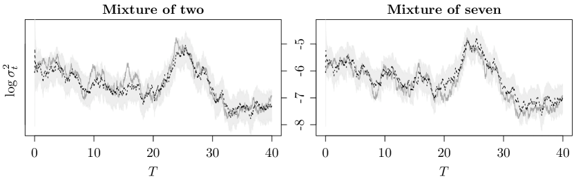
Figure 2: Comparison of the true $\log\sigma^{2}_{t}$ path (solid line) and estimated (dotted line) with a mixture of two normal distributions (left) and mixture of seven normal distributions (right). Shaded in gray is a 95% confidence interval for both estimations.

2.4.3 CKLS with stochastic volatility and correlated errors

We incorporate leverage effect to the CKLS-OU model in (23) by considering correlated Wiener processes, given by

$$\mathop{}\!\mathrm{d}r_{t} =(\alpha-\beta r_{t})\mathop{}\!\mathrm{d}t+\sigma_{t}r_{t}^{\gamma}\mathop{}\!\mathrm{d}W_{1,t},$$ (25)

$$\mathop{}\!\mathrm{d}\log\sigma_{t}^{2} =(\theta_{0}-\theta_{1}\log\sigma_{t}^{2})\mathop{}\!\mathrm{d}t+\xi\mathop{}\!\mathrm{d}W_{2,t},$$

$$\mathop{}\!\mathrm{d}W_{1,t}\mathop{}\!\mathrm{d}W_{2,t} =\rho\mathop{}\!\mathrm{d}t.$$

with $\rho\in[-1,1]$.

Let $e_{t_{i}}$ be the residuals from the linear regression, $e_{t_{i}}=\left[r_{t_{i}}-\alpha\Delta+(1-\beta\Delta)r_{t_{i-1}}\right]/\sqrt{\Delta}=\sigma_{t_{i_{1}}}r_{t_{i_{1}}}^{\gamma}\varepsilon_{1,t_{i}}$ with $\varepsilon_{1,t_{i}}$ standard Gaussian distributed, the discretized version of (25), setting $y_{t_{i}}=\log e_{t_{i}}^{2}$ and $h_{t_{i}}=\log\sigma_{t_{i}}^{2}$, is

$$y_{t_{i}} =h_{t_{i-1}}+2\gamma\log r_{t_{i-1}}+v_{t_{i}},\qquad v_{t_{i}}\sim\log\chi^{2},$$ (26)

$$h_{t_{i}} =\phi_{0}+\phi_{1}h_{t_{i-1}}+w_{t_{i}},\qquad w_{t_{i}}\sim N(0,\sigma_{w}^{2}),$$

where $\phi_{0}=\theta_{0}\Delta$, $\phi_{1}=1-\theta_{1}\Delta$, $w_{t_{i}}=\xi\sqrt{\Delta}\varepsilon_{2,t_{i}}$, $\varepsilon_{2,t_{i}}\sim N(0,1)$, and $\sigma_{w}^{2}=\Delta\xi^{2}$, with $i=0,1,\dots,n-1$. But because of the logarithmic and square transformation ($v_{t_{i}}=\log\varepsilon_{1,t_{i}}^{2}$), we can not retain the correlation between $\varepsilon_{1,t_{i}}$ and $w_{t_{i}}$, that is, $\mathrm{Cor}\{\varepsilon_{1,t_{i}},\varepsilon_{2,t_{i}}\}=\rho$. To overcome this problem, Artigas and Tsay, (2004) proposed maintaining the leverage effect by defining $\eta_{t_{i}}=\rho w_{t_{i}}+\tilde{\eta}_{t_{i}}$, where $\tilde{\eta}_{t_{i}}$ is a normal random variable independent of $\varepsilon_{1,t_{i}}$ and $\mathbb{V}\textnormal{ar}\left[\tilde{\eta}_{t_{i}}\right]=\sigma_{w}^{2}(1-\rho)^{2}$. Note that

$$\begin{pmatrix}\varepsilon_{1,t_{i}}\\ \eta_{t_{i}}\end{pmatrix}\sim N(\mu,\Sigma),$$

where

$$\mu=\begin{pmatrix}0\\ 0\end{pmatrix},\qquad\Sigma=\begin{pmatrix}1&\rho\sigma_{w}\\ \rho\sigma_{w}&\sigma_{w}^{2}\end{pmatrix},$$

therefore, $\Sigma_{\eta_{t_{i}}\mid\varepsilon_{1,t_{i}}}=\sigma_{w}^{2}-\rho^{2}\sigma_{w}^{2}$. The state-space equations for the Kalman Filter algorithm can be written as

$$y_{t_{i}} =h_{t_{i-1}}+2\gamma\log r_{t_{i-1}}+v_{t_{i}},$$ (27)

$$h_{t_{i}} =\phi_{0}+\phi_{1}h_{t_{i-1}}+\eta_{t_{i}},$$

with $\eta_{t_{i}}=\rho\sigma_{w}^{2}\varepsilon_{1,t_{i}}+\tilde{\eta}_{t_{i}}$ and $\tilde{\eta}_{t_{i}}\sim N\big{(}0,\sigma_{w}^{2}(1-\rho)^{2}\big{)}$. Substituting $\varepsilon_{1,t_{i}}=e_{t_{i}}\exp\big{(}-h_{t_{i-1}}/2\big{)}r_{t_{i-1}}^{-\gamma}$ in the state equation in (27), we have the modified state equation

$$h_{t_{i}}=\phi_{0}+\phi_{1}h_{t_{i-1}}+\rho\,\sigma_{w}e_{t_{i}}\exp\bigg{(}-\frac{h_{t_{i-1}}}{2}\bigg{)}r_{t_{i-1}}^{-\gamma}+\tilde{\eta}_{t_{i}}=G(h_{t_{i-1}})+\tilde{\eta}_{t_{i}}.$$

This equation is nonlinear, meaning that the filtering equations in (16)–(17) are no longer applicable. However, Artigas and Tsay, (2004) proposed approximating the system by using a time-varying linear Kalman Filter, thus, we modify

$$P_{t_{i+1}\mid t_{i}}=g\big{(}h_{t_{i}\mid t_{i}}\big{)}^{2}P_{t_{i}\mid t_{i}}+\sigma_{w}^{2}(1-\rho^{2}),$$

where

$$g\big{(}h_{t_{i}\mid t_{i}}\big{)}=\frac{\partial G(x)}{\partial x\mathrel{\big{|}}_{x=h_{t_{i}\mid t_{i}}}}=\phi_{1}-\frac{1}{2}\rho\,\sigma_{w}e_{t_{i+1}}\exp\bigg{(}-\frac{h_{t_{i}}}{2}\bigg{)}r_{t_{i}}^{-\gamma}.$$

We used this modification of the filtering equations to do a simulation study for the CKLS-OU model with leverage effect, introduced in (25). We generated a thousand random sample paths $\{r_{i\Delta}\}_{i=0}^{n}$, discarding the first 1000 observations as a burn-in period, with weekly frequency for sample sizes $n\in\{520,1040,2080\}$, that is $T=\{10,20,40\}$ years, and parameters $\boldsymbol{\theta}=(\alpha,\beta,\gamma,\phi_{0},\phi_{1},\xi,\rho)^{\prime}=(0.04,0.6,1.5,-0.010,0.998,0.4,-0.5)^{\prime}$.

Tables 8–10 contain the mean, variance and mean squared error for the estimations obtained using the Kalman Filter with a mixture of two (left) and seven (right) Gaussian distributions, for $T=10,20$ and $40$ years, respectively. Both methods perform similarly, achieving the seven mixture method slightly more accurate estimations, as the MSE is lower. However, they perform poorly when estimating the correlation $\rho$, even with 40 years of weekly data.

		Kalman Filter (2)				Kalman Filter (7)
	True	Mean	Var	MSE		Mean	Var	MSE
$\alpha$	0.04	0.0542	0.0007	0.0009		0.0542	0.0007	0.0009
$\beta$	0.6	0.8127	0.1600	0.2053		0.8127	0.1600	0.2053
$\gamma$	1.5	1.5812	0.0560	0.0626		1.5350	0.0443	0.0455
$\phi_{0}$	-0.010	-0.3974	2.2753	2.4257		-0.2071	2.0415	2.0805
$\phi_{1}$	0.998	0.9330	0.1030	0.1072		0.9839	0.0584	0.0586
$\xi$	0.4	0.6656	0.8315	0.9021		0.5251	0.2638	0.2795
$\rho$	-0.5	-0.1697	0.1295	0.2386		-0.1855	0.0854	0.1843

Table 8: Parameter estimates for the discretized version of (25), as in (26), for the Kalman Filter algorithm with a mixture of two (left) and seven (right) Gaussian distributions, with weekly data and $n=520$, which corresponds to $T=10$ years.

		Kalman Filter (2)				Kalman Filter (7)
	True	Mean	Var	MSE		Mean	Var	MSE
$\alpha$	0.04	0.0485	0.0004	0.0004		0.0485	0.0004	0.0004
$\beta$	0.6	0.7282	0.0836	0.1000		0.7282	0.0836	0.1000
$\gamma$	1.5	1.6027	0.0827	0.0933		1.5392	0.0327	0.0343
$\phi_{0}$	-0.010	-0.2130	1.8248	1.8662		-0.0335	0.5314	0.5320
$\phi_{1}$	0.998	0.9842	0.0355	0.0357		1.0155	0.0171	0.0174
$\xi$	0.4	0.5286	0.2646	0.2811		0.5591	0.1389	0.1642
$\rho$	-0.5	-0.1418	0.0694	0.4813		-0.1742	0.0238	0.4784

Table 9: Simulation for weekly data and $n=1040$ ($T=20$ years).

		Kalman Filter (2)				Kalman Filter (7)
	True	Mean	Var	MSE		Mean	Var	MSE
$\alpha$	0.04	0.0452	0.0002	0.0003		0.0452	0.0002	0.0003
$\beta$	0.6	0.6781	0.0502	0.0563		0.6781	0.0502	0.0563
$\gamma$	1.5	1.5675	0.1212	0.1257		1.5232	0.0336	0.0342
$\phi_{0}$	-0.010	-0.2519	2.3199	2.3785		-0.0225	0.7764	0.7766
$\phi_{1}$	0.998	0.9776	0.0254	0.0258		1.0154	0.0120	0.0123
$\xi$	0.4	0.5446	0.1866	0.2075		0.5809	0.0767	0.1094
$\rho$	-0.5	-0.2564	0.0925	0.6647		-0.2469	0.0588	0.6167

Table 10: Simulation for weekly data and $n=2080$ ($T=40$ years).

3 A GoF test for diffusion processes

In this section, two goodness-of-fit test are introduced. Based on the methodology developed by Stute, (1997) and extending the goodness-of-fit test presented in Monsalve-Cobis et al., (2011), we propose a test for the parametric form of the drift and diffusion functions of the continuous-time stochastic volatility models in (2)–(3). The test for the drift function is based on the integrated regression function of the process, while the test for diffusion function relies on the integrated volatility function. The test statistics are based on a distance of the resulting residual marked empirical processes from their expected zero mean, measured by Kolmogorov-Smirnov and Cramér-von Mises functionals. In both tests, the distribution of the statistic is approximated by bootstrap techniques.

3.1 Test for the volatility function

The goodness-of-fit test for the parametric form of the volatility function $\nu_{1}(\cdot)$ in (2)–(3) under the assumption that the null hypothesis

$$\mathcal{H}_{0\nu}\colon\nu_{1}\in\{\nu_{1}(\cdot,\boldsymbol{\theta})\colon\boldsymbol{\theta}\in\Theta\}$$

holds, is based on the integrated conditional variance function

$$V_{0}(r,x)=\int_{-\infty}^{r}\int_{-\infty}^{x}\nu_{1}^{2}(u,v)\mathop{}\!\mathrm{d}F_{\boldsymbol{\theta}}(u,v)=\mathbb{E}\big{[}\nu_{1}^{2}(r_{t},\boldsymbol{\theta})\mathbbm{1}_{\{r_{t}\leq r,\sigma^{2}_{t}\leq x\}}\big{]},$$

with $r,x\in\mathbb{R}$ and where $F$ is the stationary distribution of $\{r_{t},\sigma_{t}^{2}\}$ and $\mathbbm{1}_{\{\cdot\}}$ the indicator function. Considering an empirical estimator of $V(r,x)$,

$$V_{0n}(r,x)=\frac{1}{n}\sum_{i=0}^{n-1}\mathbbm{1}_{\{r_{t_{i}}\leq r,\sigma^{2}_{t_{i}}\leq x\}}\left(\frac{r_{t_{i+1}}-r_{t_{i}}}{\Delta}-m_{1}(r_{t_{i}},\hat{\boldsymbol{\theta}})\right)^{2},$$

and assuming that $\hat{\boldsymbol{\theta}}$ is an root-$n$ consistent estimator of the true parameter $\boldsymbol{\theta}$, the goodness-of-fit test is based on the empirical process

$$R_{n}^{\nu}(r,x)=\frac{1}{\sqrt{n}}\sum_{i=0}^{n-1}\mathbbm{1}_{\{r_{t_{i}}\leq r,\hat{\sigma}^{2}_{t_{i}}\leq x\}}\left[\left(\frac{r_{t_{i+1}}-r_{t_{i}}}{\Delta}-m_{1}(r_{t_{i}},\hat{\boldsymbol{\theta}})\right)^{2}-\frac{\hat{\sigma}^{2}_{t_{i}}\nu_{1}^{2}(r_{t_{i}},\hat{\boldsymbol{\theta}})}{\Delta}\right],$$

with $r,x\in\mathbb{R}$ and $\hat{\sigma}^{2}_{t}$ an estimate of the volatility. A continuous functional $\Psi(\cdot)$ of the empirical process can be considered to define the test statistic $U_{n}=\Psi(R_{n}^{\nu})$. The null hypothesis is rejected if $U_{n}>c_{1-\alpha}$, where $c_{1-\alpha}$ is the critical value for the $\alpha$-level test,

$$\mathbb{P}\left(\Psi(R_{n}^{\nu})>c_{1-\alpha}\mid\mathcal{H}_{0\nu}\right)=\alpha.$$

The critical value $c_{1-\alpha}$ can be determined by approximating the distribution of the process $R_{n}^{\nu}$ using bootstrap techniques (Stute et al.,, 1998). Let $c^{*}_{1-\alpha}$ denote the bootstrap approximated critical value $c_{1-\alpha}$, so that $\mathbb{P}^{*}\left(\Psi(R_{n}^{\nu*})>c^{*}_{1-\alpha}\mid\mathcal{H}_{0\nu}\right)=\alpha$, where $\mathbb{P}^{*}$ is the probability measure generated by the bootstrap sample and the bootstrap counterpart of the empirical process $R_{n}^{\nu}(\cdot)$ is given by

$$R_{n}^{\nu*}(r,x)=\frac{1}{\sqrt{n}}\sum_{i=0}^{n-1}\mathbbm{1}_{\{r_{t_{i}}^{*}\leq r,\hat{\sigma}^{*2}_{t_{i}}\leq x\}}\left[\left(\frac{r_{t_{i+1}}^{*}-r_{t_{i}}^{*}}{\Delta}-m_{1}(r_{t_{i}}^{*},\hat{\boldsymbol{\theta}}^{*})\right)^{2}-\frac{\hat{\sigma}^{*2}_{t_{i}}\nu_{1}^{2}(r_{t_{i}}^{*},\hat{\boldsymbol{\theta}}^{*})}{\Delta}\right],$$

with $\hat{\boldsymbol{\theta}}^{*}$ an estimator obtained from the bootstrapped sample $\{(r_{t_{i}}^{*},\sigma_{t_{i}}^{*2})\}$ (the procedure to obtain the resamples is defined in Section 3.3). Bootstrap replicates of the statistic $U_{n}^{*j}=\Psi\big{(}R_{n}^{\nu*}(r,x)\big{)}$, for $j=1,\dots,B$, are obtained and, using Monte Carlo techniques, the critical value is approximated with the statistic of order $\lceil B(1-\alpha)\rceil$ from the $B$ bootstrap replicates, that is, $c^{*}_{1-\alpha}=U_{n}^{*\lceil B(1-\alpha)\rceil}$ (see Algorithm 4 for a summary of the bootstrap procedure to approximate the critical value $c_{1-\alpha}$). The null hypothesis $\mathcal{H}_{0\nu}$ is rejected if $U_{n}>c^{*}_{1-\alpha}$.

The functional $\Psi(\cdot)$ can take the form of the Kolmogorov-Smirnov (KS) and Cramér-von Mises (CvM) criteria, so that the statistics can be expressed as

$$U_{n}^{KS} \coloneqq\sup\limits_{r,x}\left|R_{n}^{\nu}(r,x)\right|,$$

$$U_{n}^{CvM} \coloneqq\int\int_{\mathbb{R}^{2}}\left(R_{n}^{\nu}(r,x)\right)^{2}F_{n}(\mathop{}\!\mathrm{d}r,\mathop{}\!\mathrm{d}x),$$

respectively, where $F_{n}$ is the empirical distribution of $\{r_{t_{i}},\hat{\sigma}^{2}_{t_{i}}\}_{i=0}^{n-1}$. The empirical $p$-value is estimated with the proportion of the B bootstrap replicates $U_{n}^{*j}$ exceeding $U_{n}$, that is,

$$\frac{\sharp\{U_{n}^{*j}>U_{n}\}}{B}.$$

3.2 Test for the drift function

Aiming to test if the parametric form of the drift function $m_{1}(\cdot)$ in (2)–(3) belongs to a certain parametric family, we establish the null hypothesis

$$\mathcal{H}_{0m}\colon m_{1}\in\{m_{1}(\cdot,\boldsymbol{\theta})\colon\boldsymbol{\theta}\in\Theta\}.$$

We propose a test based on the integrated regression function $I(x)=\mathbb{E}\left[Y\mathbbm{1}_{\{X\leq x\}}\right]=\int_{-\infty}^{x}m(y)\mathop{}\!\mathrm{d}F(y)$, where $F$ is the marginal distribution function of $X$. An empirical estimator of the integrated regression function for the model (2)–(3) is given by

$$I_{n}(r)=\frac{1}{n}\sum_{i=0}^{n-1}\mathbbm{1}_{\{r_{t_{i}}\leq r\}}\frac{r_{t_{i+1}}-r_{t_{i}}}{\Delta},$$

and an estimator under the null hypothesis $\mathcal{H}_{0m}$ is

$$I_{0n}(r)=\frac{1}{n}\sum_{i=0}^{n-1}\mathbbm{1}_{\{r_{t_{i}}\leq r\}}m_{1}(r_{t_{i}},\hat{\boldsymbol{\theta}}).$$

The goodness-of-fit test compares the estimated integrated regression function $I_{n}(\cdot)$ with the estimation obtained under the null hypothesis, that is, $I_{0n}(\cdot)$. Therefore, the test is defined by the process

$$R_{n}^{m}(r)=\frac{1}{\sqrt{n}}\sum_{i=0}^{n-1}\mathbbm{1}_{\{r_{t_{i}}\leq r\}}\left(\frac{r_{t_{i+1}}-r_{t_{i}}}{\Delta}-m_{1}(r_{t_{i}},\hat{\boldsymbol{\theta}})\right),$$

with $r\in\mathbb{R}$ and where $\hat{\boldsymbol{\theta}}$ is a $\sqrt{n}$-consistent estimator of the true parameter vector $\boldsymbol{\theta}$. As in the previous test, a continuous functional $\Psi(\cdot)$ can be considered to define the statistic $T_{n}=\Psi(R_{n}^{m})$, such as the Kolmogorov-Smirnov and Cramér-von Mises criteria,

$$T_{n}^{KS}\coloneqq\sup\limits_{r}\left|R_{n}^{m}(r)\right|\qquad\text{and}\qquad T_{n}^{CvM}\coloneqq\int_{\mathbb{R}}R_{n}^{m}(r)^{2}F_{n}(\mathop{}\!\mathrm{d}r),$$

respectively, with $F_{n}$ the empirical distribution function of $\{r_{t_{i}}\}_{i=0}^{n-1}$. The null hypothesis is rejected if $T_{n}>c_{1-\alpha}$. Again, the critical value $c_{1-\alpha}$ can be approximated by its bootstrap counterpart $c^{*}_{1-\alpha}$, such that $\mathbb{P}^{*}\left(\Psi(R_{n}^{m*})>c^{*}_{1-\alpha}\mid\mathcal{H}_{0m}\right)=\alpha$ with

$$R_{n}^{m*}(r)=\frac{1}{\sqrt{n}}\sum_{i=0}^{n-1}\mathbbm{1}_{\{r_{t_{i}}\leq r\}}\left(u^{*}_{t_{i}}-m_{1}(r_{t_{i}},\hat{\boldsymbol{\theta}}^{*})\right),$$

where $u_{t_{i}}=(r_{t_{i+1}}-r_{t_{i}})/\Delta$ and $u_{t_{i}}^{*}=m_{1}(r_{t_{i}},\hat{\boldsymbol{\theta}})+e_{t_{i}}^{*}$ is obtained sampling the innovations $e_{t_{i}}$ with the algorithm introduced in Section 3.3, and the bootstrap estimator $\hat{\boldsymbol{\theta}}^{*}$ is calculated from the bootstrap sample $\{(r_{t_{i}}^{*},\sigma_{t_{i}}^{*2})\}$. The approximated critical value $c^{*}_{1-\alpha}$ is achieved by means of Monte Carlo techniques, that is, $c^{*}_{1-\alpha}=T_{n}^{*\lceil B(1-\alpha)\rceil}$, with the order $\lceil B(1-\alpha)\rceil$ statistic from $B$ bootstrap replicates $\big{\{}T_{n}^{*j}=\Psi(R_{n}^{m*})\big{\}}_{j=1}^{B}$. As explained in the previous test, the empirical $p$-value is the proportion of the $B$ bootstrap replicates $T_{n}^{*j}$ exceeding $T_{n}$, $\sharp\{T_{n}^{*j}>T_{n}\}/B$.

3.3 Bootstrap resampling procedure

The estimation of $\boldsymbol{\theta}$ and the bootstrap sample $\{(r_{t_{i}}^{*},\sigma_{t_{i}}^{*2})\}$ can be obtained with the Kalman Filter algorithm (Shumway and Stoffer,, 2000). Given the filtering equations introduced in (16)–(17), the bootstrap resample algorithm for model (2)–(3) can be implemented as follows. First, calculate the residuals from the linear regression $e_{t_{i}}=[r_{t_{i}}-m_{1}(r_{t_{i}},\boldsymbol{\theta})]/\sqrt{\Delta}=\sigma_{t_{i}}\nu_{1}(r_{t_{i}},\boldsymbol{\theta})\varepsilon_{1,t_{i}}$; second, define $y_{t_{i}}=\log e_{t_{i}}^{2}\quad\text{and}\quad h_{t_{i}}=\log\sigma_{t_{i}}^{2}$ to linearize the space equation, therefore we have the following space-state equations,

$$y_{t_{i}} =h_{t_{i}}+\log\nu_{1}(r_{t_{i}},\boldsymbol{\theta})^{2}+v_{t_{i}},\qquad\quad v_{t_{i}}\sim\log\chi^{2}_{1},$$

$$h_{t_{i}} =m_{2}(h_{t_{i}},\boldsymbol{\theta})+w_{t_{i}},\qquad\quad w_{t_{i}}\sim N(0,\sigma_{w}^{2}),$$

with $w_{t_{i}}=\nu_{2}(h_{t_{i}},\boldsymbol{\theta})\sqrt{\Delta}\,\varepsilon_{2,t_{i}}$, $\varepsilon_{2,t_{i}}\sim N(0,1)$ and $\sigma_{w}^{2}=\Delta\nu_{2}(h_{t_{i}},\boldsymbol{\theta})^{2}$. Given the filtering equations (16)–(17) we have

$$y_{t_{i}}=h_{t_{i}\mid{t_{i-1}}}+\log\nu_{1}(r_{t_{i-1}},\boldsymbol{\theta})^{2}+\pi_{0,t_{i}}\epsilon_{0,t_{i}}+\pi_{1,t_{i}}(\epsilon_{1,t_{i}}+\mu_{1}).$$

Let $\hat{\boldsymbol{\theta}}$ denote the maximum likelihood estimator of the true parameter $\boldsymbol{\theta}$, $\hat{\boldsymbol{\theta}}=\operatorname*{\arg\max}\limits_{\Theta}\ln\mathcal{L}_{Y}(\boldsymbol{\theta})$, by means of the Kalman Filter algorithm, and $\epsilon_{j,t_{i}}$, with $\mathbb{V}\mathrm{ar}\left[\epsilon_{j,t_{i}}\right]=\hat{\Sigma}_{j,t_{i}}$, the innovations and the innovations variance obtained by running the filter under $\hat{\boldsymbol{\theta}}$. To implement the bootstrap algorithm we consider the standardized innovations

$$\tilde{\epsilon}_{j,t_{i}}=\hat{\Sigma}_{j,t_{i}}^{-1/2}\epsilon_{j,t_{i}},\quad\text{ for }j=0,1,$$

and sample with replacement from $\{\tilde{\epsilon}_{j,t_{i}}\}_{i=0}^{n-1}$ to obtain the bootstrap sample of standardized innovations $\{\tilde{\epsilon}_{j,t_{i}}^{*}\}_{i=0}^{n-1}$. We then generate the bootstrap sample $\{(y_{t_{i}}^{*},h_{t_{i}}^{*})\}_{i=0}^{n-1}$ with

$$h_{t_{i+1}}^{*} =m_{2}(h_{t_{i}\mid t_{i-1}},\hat{\boldsymbol{\theta}})+\hat{\pi}_{0,t_{i}}K_{0,t_{i}}\hat{\Sigma}_{0,t_{i}}^{1/2}\tilde{\epsilon}_{0,t_{i}}^{*}+\hat{\pi}_{1,t_{i}}K_{1,t_{i}}\hat{\Sigma}_{1,t_{i}}^{1/2}\tilde{\epsilon}_{1,t_{i}}^{*},$$ (28)

$$y_{t_{i}}^{*} =h_{t_{i}\mid t_{i-1}}+\log\nu_{1}(r_{t_{i}},\hat{\boldsymbol{\theta}})^{2}+\hat{\pi}_{1,t_{i}}\hat{\mu}_{1}+\hat{\pi}_{0,t_{i}}\hat{\Sigma}_{0,t_{i}}^{1/2}\tilde{\epsilon}_{0,t_{i}}^{*}+\hat{\pi}_{1,t_{i}}\hat{\Sigma}_{1,t_{i}}^{1/2}\tilde{\epsilon}_{1,t_{i}}^{*},$$

where $r_{t_{i}}$ remains fixed and the bootstrapped dataset is given by $\exp(y_{t_{i}}^{*})=e_{t}^{2*}$. Algorithm 4 summarizes the bootstrap procedure to approximate the critical value $c_{1-\alpha}$.

Algorithm 4 (Bootstrap resampling procedure).

The critical value $c_{1-\alpha}$ can be approximated with the following bootstrap procedure:

1. Obtain the maximum likelihood estimator of the true parameter $\boldsymbol{\theta}$, that is, $\hat{\boldsymbol{\theta}}=\operatorname*{\arg\max}\limits_{\Theta}\ln\mathcal{L}_{Y}(\boldsymbol{\theta})$, by means of the Kalman Filter algorithm introduced in (18).

2. Construct the bootstrap sample $\{(y_{t_{i}}^{*},\sigma_{t_{i}}^{*2})\}_{i=0}^{n-1}$ as in (28).

3. Estimate the parameter vector $\hat{\boldsymbol{\theta}}^{*}$ from the bootstrap resample $\{(y_{t_{i}}^{*},\sigma_{t_{i}}^{*2})\}_{i=0}^{n-1}$ obtained in Step 2.

4. Compute the bootstrap version of the process $R_{n}^{\nu*}(r,x)$ or $R_{n}^{m*}(r)$, for $r,x\in\mathbb{R}$.

5. Determine $U_{n}^{*}=\Psi\big{(}R_{n}^{\nu*}(r,x)\big{)}$ or $T_{n}^{*}=\Psi\big{(}R_{n}^{m*}(r)\big{)}$.

6. Repeat $B$ times the previous Steps 2–5 to obtain $j=1,\dots,B$, bootstrap replicates $U_{n}^{*j}$ or $T_{n}^{*j}$.

7. Approximate the critical value $\hat{c}^{*}_{1-\alpha}=U_{n}^{*\lceil B(1-\alpha)\rceil}$ or $\hat{c}^{*}_{1-\alpha}=T_{n}^{*\lceil B(1-\alpha)\rceil}$.

4 Simulation study

In this Section, a simulation study to illustrate the finite sample properties of the tests was conducted under different settings, for both the drift and volatility goodness-of-fit tests. As to our knowledge, the tests available in the literature for continuous-time stochastic volatility models do not test the same null hypothesis as our test, that is, the parametric form of the diffusion function, we are not including a comparison with other procedures.

4.1 Drift test

The performance of the goodness-of-fit test for the parametric form of the drift function introduced in Section 3.2, regarding size and power, is illustrated by means of a simulation study. We test the null hypothesis that the drift function $m_{1}(\cdot)$ of the SDE in (2)–(3) belongs to a certain parametric family,

$$\mathcal{H}_{0m}\colon m_{1}\in\{m_{1}(\cdot,\boldsymbol{\theta})\colon\boldsymbol{\theta}\in\Theta\}.$$

We consider the CKLS-OU model as the null hypothesis and to evaluate the power of the test we use a series of alternative models indexed by the parameter $\rho$ of the non-linear function $\rho_{m}(r_{t})=\rho(1-r_{t}^{\rho})$,

$$\mathop{}\!\mathrm{d}r_{t} =\big{(}\alpha-\beta r_{t}+\rho(1-r_{t}^{\,\rho})\big{)}\mathop{}\!\mathrm{d}t+\sigma_{t}r_{t}^{\gamma}\mathop{}\!\mathrm{d}W_{1,t},$$

$$\mathop{}\!\mathrm{d}\ln\sigma_{t}^{2} =(\theta_{0}-\theta_{1}\log\sigma_{t}^{2})\mathop{}\!\mathrm{d}t+\xi\mathop{}\!\mathrm{d}W_{2,t},$$

with $\rho\in\{0,0.07,0.09,0.10,0.125,0.15\}$, where $\rho=0$ under the null hypothesis. The parameter vector for the data generating process (DGP) is $\boldsymbol{\theta}=(\alpha,\beta,\gamma,\theta_{0},\theta_{1},\xi)^{\prime}=(0.04,0.6,1.5,-0.7,0.1,0.4)$. The process was generated with weekly frequency ($\Delta=1/52$) for different sample sizes $n\in\{500,1000,1500,2000\}$ and the first thousand observations were discarded as a burn-in period. The rate of rejection ($\hat{\alpha}$) is calculated based on $1000$ Monte Carlo replicates and $B=1000$ bootstrap resamples (see Algorithm 4) for the Kolmogorov-Smirnov ($\hat{\alpha}_{\text{KS}}$) and Cramér-von Mises $(\hat{\alpha}_{\text{CvM}}$) criteria.

Table 11 show the size (first row) and power of the goodness-of-fit test for the drift function $m_{1}(\cdot)$ for the null hypothesis that the drift function follows the CKLS-OU parametric form, that is, $\mathcal{H}_{0m}\colon m_{1}(r_{t},\boldsymbol{\theta})=\alpha-\beta r_{t}$, with $\alpha=0.05$. Regarding the size, the tests are well calibrated as both rejection rates are very close to the nominal level $\alpha$. The behavior of the power, on the other hand, shows an increase with the sample size, as expected, and the higher the value of $\rho$, the further we depart from the null hypothesis, obtaining higher rejection rates.

		$\hat{\alpha}_{\text{KS}}$					$\hat{\alpha}_{\text{CvM}}$
DGP		500	1000	1500	2000		500	1000	1500	2000
$\rho=$ 0		0.047	0.043	0.045	0.044		0.054	0.051	0.060	0.056
$\rho=$ 0.07		0.102	0.186	0.203	0.301		0.169	0.267	0.298	0.356
$\rho=$ 0.09		0.301	0.305	0.356	0.456		0.314	0.364	0.448	0.508
$\rho=$ 0.10		0.365	0.456	0.481	0.526		0.441	0.528	0.560	0.606
$\rho=$ 0.125		0.523	0.618	0.669	0.703		0.531	0.636	0.682	0.747
$\rho=$ 0.15		0.790	0.848	0.869	0.901		0.785	0.864	0.907	0.923

Table 11: Size ($\rho=0$) and power simulation for the CKLS-OU model drift test, with $\alpha=0.05$, for the null hypothesis $\mathcal{H}_{0}\colon m_{1}(r_{t},\boldsymbol{\theta})=\alpha-\beta r_{t}$, under different alternative scenarios $m_{1}(r_{t},\boldsymbol{\theta})=\big{(}\alpha-\beta r_{t}+\rho(1-r_{t}^{\,\rho})\big{)}$, for $\rho\in\{0,0.07,0.09,0.10,0.125,0.15\}$.

4.2 Volatility test

The study of the finite sample properties of the goodness-of-fit test for the parametric form of the volatility function introduced in Section 3.1 is accomplish with a simulations study, testing both simple and composite null hypotheses. We test the null hypothesis that the diffusion function $\nu_{1}(\cdot)$ of the continuous-time model in (2)–(3) belongs to a certain parametric family, that is,

$$\mathcal{H}_{0\nu}\colon\nu_{1}\in\{\nu_{1}(\cdot,\boldsymbol{\theta})\colon\boldsymbol{\theta}\in\Theta\},$$

for the composite hypothesis. We consider three different models under the null hypothesis, which are described in Table 12, and, to asses the performance of the power of the test, we take the CKLS-OU model and create a series of alternative scenarios by adding a non-linear function to the diffusion function $\nu_{1}(\cdot)$

$$\mathop{}\!\mathrm{d}r_{t} =(\alpha-\beta r_{t})\mathop{}\!\mathrm{d}t+\big{[}\sigma_{t}r_{t}^{\gamma}+\rho(1-r_{t}^{\,\rho})\big{]}\mathop{}\!\mathrm{d}W_{1,t},$$

$$\mathop{}\!\mathrm{d}\ln\sigma_{t}^{2} =(\theta_{0}-\theta_{1}\log\sigma_{t}^{2})\mathop{}\!\mathrm{d}t+\xi\mathop{}\!\mathrm{d}W_{2,t},$$

with $\rho\in\{0.007,0.01,0.02,0.04\}$, where $\rho=0$ under the null hypothesis (scenario CKLS-OU in Table 12). The processes were generated with weekly frequency ($\Delta=1/52$) for sample sizes $n\in\{500,1000,1500,2000\}$ and the first thousand observations were discarded. The rate of rejection ($\hat{\alpha}$) is calculated based on $1000$ Monte Carlo replicates and $B=1000$ bootstrap resamples (see Algorithm 4) for the Kolmogorov-Smirnov ($\hat{\alpha}_{\text{KS}}$) and Cramér-von Mises $(\hat{\alpha}_{\text{CvM}}$) criteria.

The size and power of the test for the simple null hypothesis will be evaluated using the CKLS-OU model ($\nu_{1}(r_{t},\boldsymbol{\theta})=r_{t}^{\gamma}$), testing the null hypothesis $\mathcal{H}_{0\nu}\colon\nu_{1}(r_{t},\boldsymbol{\theta})=r_{t}^{1.5}$ for a set of values $\gamma\in\{1.5,1.25,1.0\}$.

Scenario	Model	Parameters
OU-OU	$\begin{array}[t]{ r @{{}={}} l }\mathop{}\!\mathrm{d}r_{t}&(\alpha-\beta r_{t})\mathop{}\!\mathrm{d}t+\sigma_{t}\mathop{}\!\mathrm{d}W_{1,t}\\ \mathop{}\!\mathrm{d}\ln\sigma_{t}^{2}&(\theta_{0}-\theta_{1}\log\sigma_{t}^{2})\mathop{}\!\mathrm{d}t+\xi\mathop{}\!\mathrm{d}W_{2,t}\end{array}$	$\begin{array}[t]{ r @{{}={}} l }\boldsymbol{\theta}&(\alpha,\beta,\gamma,\theta_{0},\theta_{1},\xi)^{\prime}\\ &(0.04,0.6,-0.7,0.1,0.4)^{\prime}\phantom{1.5,}\end{array}$
CKLS-null	$\begin{array}[t]{ r @{{}={}} l }\mathop{}\!\mathrm{d}r_{t}&(\alpha-\beta r_{t})\mathop{}\!\mathrm{d}t+\sigma_{t}r_{t}^{\gamma}\mathop{}\!\mathrm{d}W_{1,t}\\ \mathop{}\!\mathrm{d}\ln\sigma_{t}^{2}&\xi\mathop{}\!\mathrm{d}W_{2,t}\hphantom{\,+\,(\theta_{0}-\theta_{1}\log\sigma_{t}^{2})\mathop{}\!\mathrm{d}t}\end{array}$	$\begin{array}[t]{ r @{{}={}} l }\boldsymbol{\theta}&(\alpha,\beta,\gamma,\xi)^{\prime}\\ &(0.04,0.6,1.5,0.4)^{\prime}\phantom{-0.7,0.1,}\end{array}$
CKLS-OU	$\begin{array}[t]{ r @{{}={}} l }\mathop{}\!\mathrm{d}r_{t}&(\alpha-\beta r_{t})\mathop{}\!\mathrm{d}t+\sigma_{t}r_{t}^{\gamma}\mathop{}\!\mathrm{d}W_{1,t}\\ \mathop{}\!\mathrm{d}\ln\sigma_{t}^{2}&(\theta_{0}-\theta_{1}\log\sigma_{t}^{2})\mathop{}\!\mathrm{d}t+\xi\mathop{}\!\mathrm{d}W_{2,t}\end{array}$	$\begin{array}[t]{ r @{{}={}} l }\boldsymbol{\theta}&(\alpha,\beta,\gamma,\theta_{0},\theta_{1},\xi)^{\prime}\\ &(0.04,0.6,1.5,-0.7,0.1,0.4)^{\prime}\end{array}$

Table 12: Scenarios under the composite null hypothesis.

Table 13 shows the empirical size and power for simple and composite hypotheses, the later under the null hypotheses for the scenarios in Table 12. Regarding the simple hypothesis test, the size (first row) is close to the nominal level $\alpha=0.05$, with a slight over rejection for the smallest sample size scenario, and the power increases with sample size and shows that the test is capable of discriminating between models with different values of $\gamma$. Focusing on the composite null hypothesis, the estimated sizes (first three rows) remain close the the true nominal level, although the smallest sample sizes show some small deviations, and the power increases both with the sample size and the value of $\rho$, which controls the level of noise added to the diffusion function.

		$\hat{\alpha}_{\text{KS}}$					$\hat{\alpha}_{\text{CvM}}$
$\mathcal{H}_{0}$	DGP	500	1000	1500	2000		500	1000	1500	2000
Simple hypothesis
$\gamma=1.50$	CKLS-OU	0.089	0.046	0.041	0.049		0.040	0.044	0.062	0.052
$\gamma=1.50$	$\gamma=1.25$	0.454	0.613	0.708	0.808		0.462	0.602	0.767	0.818
$\gamma=1.50$	$\gamma=1.00$	0.734	0.884	0.957	0.986		0.649	0.873	0.974	0.988
Composite hypothesis
$\nu_{1}(r_{t},\boldsymbol{\theta})=1$	OU-OU	0.037	0.046	0.046	0.058		0.045	0.051	0.032	0.064
$\nu_{1}(r_{t},\boldsymbol{\theta})=r_{t}^{\gamma}$	CKLS-null	0.033	0.048	0.038	0.057		0.035	0.051	0.034	0.063
$\nu_{1}(r_{t},\boldsymbol{\theta})=r_{t}^{\gamma}$	CKLS-OU	0.040	0.047	0.041	0.047		0.044	0.053	0.034	0.041
$\nu_{1}(r_{t},\boldsymbol{\theta})=r_{t}^{\gamma}$	$\rho=$ 0.007	0.125	0.177	0.206	0.331		0.099	0.148	0.190	0.303
$\nu_{1}(r_{t},\boldsymbol{\theta})=r_{t}^{\gamma}$	$\rho=$ 0.01	0.364	0.468	0.641	0.657		0.304	0.423	0.578	0.619
$\nu_{1}(r_{t},\boldsymbol{\theta})=r_{t}^{\gamma}$	$\rho=$ 0.02	0.490	0.644	0.710	0.796		0.415	0.581	0.674	0.701
$\nu_{1}(r_{t},\boldsymbol{\theta})=r_{t}^{\gamma}$	$\rho=$ 0.04	0.527	0.766	0.870	0.951		0.491	0.620	0.714	0.819

Table 13: Size and power simulation for the volatility function tests, with $\alpha=0.05$, considering simple and composite null hypotheses. Under $\mathcal{H}_{0}$, rejection rates are boldfaced if they lie outside a 95%-confidence interval for the nominal level $\alpha$.

5 Real data applications

In this section, we consider the Euribor (Euro Interbank Offered Rate) interest rate series corresponding to four maturities (three, six, nine and twelve months), see Figure 3. The four datasets expand from October 15^th 2001 to December 30^th 2005 (sample size of $n=1\,077$). We fit the CKLS with stochastic volatility in (24), as different models can be nested within this unrestricted model, and test the goodness of fit of the model in terms of the parametric form of the volatility function.

Table 14 shows the parameter estimations for the CKLS-OU model, with the associated standard error in parentheses. The values verify the trait usually associated with interest rate time series, that is, persistence, both for the interest rate $r_{t}$ and volatility $\sigma_{t}$ equations. Regarding the parameter $\gamma$, which controls the relationship between the interest rate level and the volatility, for all maturities we have $\gamma>1$. This indicates that the volatility tends to increase as the interest rate $r_{t}$ raises.

(a) Euribor 3 months.

(b) Euribor 6 months.

(c) Euribor 9 months.

(d) Euribor 12 months.

Figure 3: Daily evolution of Euribor series for the time period between October 15^th 2001 and December 30^th 2005. Sample size for each dataset is $n=1\,077$.

Regarding the goodness-of-fit test, Table 15 shows the $p$-values for the parametric form of the volatility function, both for the Kolmogorov-Smirnov and Cramér-von Mises statistics, which exhibit minor discrepancies. In López-Pérez et al., (2021) the same datasets were used to fit a CKLS model with deterministic volatility function and the null hypothesis for the parametric form of the diffusion function was strongly rejected for the four maturities. However, when considering a more flexible diffusion function with stochastic volatility, we do not reject the null hypothesis, suggesting that a model that incorporates stochastic volatility may adequately explain the dynamics of the series. Rejecting a deterministic volatility function in favor of a stochastic function indicates that the volatility evolution is not exclusively tied to the level of the short rate, but rather the process is governed by dynamic factors. This was discussed in the financial literature (see Ait-Sahalia,, 1996; Brenner et al.,, 1996; Andersen and Lund, 1997a, ; Koedijk et al.,, 1997; Gallant and Tauchen,, 1998), where less restrictive models were proposed, including the two-factor model or even multi-factor models of the short rate (Andersen and Lund, 1997b, ).

Parameters:	$\alpha$	$\beta$	$\gamma$	$\phi_{0}$	$\phi_{1}$	$\xi$
3 months	$1.6546$	$0.7733$	$1.6483$	$-0.2821$	$0.9674$	$7.2056$
	$(0.5980)$	$(0.2631)$	$(0.6711)$	$(0.1696)$	$(0.0177)$	$(1.7736)$
6 months	$1.5139$	$0.6813$	$1.4219$	$-0.0812$	$0.9878$	$2.4606$
	$(0.7567)$	$(0.3214)$	$(0.5848)$	$(0.0728)$	$(0.0103)$	$(0.8608)$
9 months	$1.6850$	$0.7218$	$1.7627$	$-0.0494$	$0.9919$	$1.3615$
	$(1.0196)$	$(0.4218)$	$(0.4122)$	$(0.0479)$	$(0.0079)$	$(0.5332)$
12 months	$1.9218$	$0.7868$	$1.6729$	$-0.0344$	$0.9937$	$1.1163$
	$(1.2384)$	$(0.4977)$	$(0.3914)$	$(0.0358)$	$(0.0066)$	$(0.4468)$

Table 14: Parameter estimates and standard errors (in parentheses) for the CKLS process with stochastic volatility, fitted to Euribor series.

Maturity	3 months	6 months	9 months	12 months
p-value Kolmogorov-Smirnov	$0.464$	$0.266$	$0.319$	$0.189$
p-value Cramér-von Mises	$0.550$	$0.215$	$0.422$	$0.113$

Table 15: $p$-values for the goodness-of-fit test for the CKLS-OU parametric form of the diffusion function.

6 Conclusions

We reviewed parametric estimation methods for two-factor continuous-time stochastic volatility models. The continuous time nature of the process does complicate the parameter estimation, as available data are registered in discrete time points. As a consequence, parameters are subject to discretization bias and this, combined with the presence of a latent factor, challenges estimation. We discussed a comparative study of three estimation methods –namely, MCMC, Kalman Filter and particle filter– under different settings. The close performance of the procedures, together with the computationally demanding and model-dependent implementation of simulation methods, makes the Kalman Filter a computational efficient estimation method to use in goodness-of-fit testing procedures. Furthermore, the space-state model structure allows to easily implement a bootstrap procedure. We proposed goodness-of-fit tests for the parametric form of the drift and volatility functions, based on a residual marked empirical process. The tests showed great power through several alternative hypotheses and was well calibrated under null hypotheses and its implementation, regarding the computation of the test statistic and the bootstrap resampling scheme, is quite straightforward. The application to real data demonstrated that the incorporation of stochastic volatility to diffusion models does capture the features of interest rate time series, unlike deterministic volatility functions, suggesting that the volatility depends on an additional factor that varies independently of the short rate level.

References

- Ait-Sahalia, (1996) Ait-Sahalia, Y. (1996). Do interest rates really follow continuous-time Markov diffusions? Working paper, Graduate School of Business, University of Chicago.
- Aït-Sahalia, (1996) Aït-Sahalia, Y. (1996). Testing continuous-time models of the spot interest rate. The Review of Financial Studies, 9(2):385–426.
- Aït-Sahalia et al., (2020) Aït-Sahalia, Y., Li, C., and Li, C. X. (2020). Maximum likelihood estimation of latent Markov models using closed-form approximations. Journal of Econometrics.
- (4) Andersen, T. G. and Lund, J. (1997a). Estimating continuous-time stochastic volatility models of the short-term interest rate. Journal of econometrics, 77(2):343–377.
- (5) Andersen, T. G. and Lund, J. (1997b). Stochastic volatility and mean drift in the short rate diffusion: sources of steepness, level and curvature in the yield curve. Working paper, L. Kellogg Graduate School of Management, Northwestern University.
- Andersen and Sørensen, (1996) Andersen, T. G. and Sørensen, B. E. (1996). GMM estimation of a stochastic volatility model: A Monte Carlo study. Journal of Business & Economic Statistics, 14(3):328–352.
- Arapis and Gao, (2006) Arapis, M. and Gao, J. (2006). Empirical comparisons in short-term interest rate models using nonparametric methods. Journal of Financial Econometrics, 4(2):310–345.
- Artigas and Tsay, (2004) Artigas, J. C. and Tsay, R. S. (2004). Efficient estimation of stochastic diffusion models with leverage effects and jumps. Working paper, Graduate School of Business, University of Chicago.
- Bates, (2006) Bates, D. S. (2006). Maximum likelihood estimation of latent affine processes. The Review of Financial Studies, 19(3):909–965.
- Black and Scholes, (1973) Black, F. and Scholes, M. (1973). The pricing of options and corporate liabilities. Journal of Political Economy, 81:637–654.
- Brenner et al., (1996) Brenner, R. J., Harjes, R. H., and Kroner, K. F. (1996). Another look at models of the short-term interest rate. Journal of Financial and Quantitative Analysis, 31(1):85–107.
- Broto and Ruiz, (2004) Broto, C. and Ruiz, E. (2004). Estimation methods for stochastic volatility models: a survey. Journal of Economic Surveys, 18(5):613–649.
- Bull, (2017) Bull, A. D. (2017). Semimartingale detection and goodness-of-fit tests. The Annals of Statistics, 45(3):1254–1283.
- Carvalho et al., (2010) Carvalho, C. M., Johannes, M. S., Lopes, H. F., and Polson, N. G. (2010). Particle learning and smoothing. Statistical Science, 25(1):88–106.
- Chan et al., (1992) Chan, K. C., Karolyi, G. A., Longstaff, F. A., and Sanders, A. B. (1992). An empirical comparison of alternative models of the short-term interest rate. The Journal of Finance, 47(3):1209–1227.
- Chen et al., (2019) Chen, Q., Hu, M., and Song, X. (2019). A nonparametric specification test for the volatility functions of diffusion processes. Econometric Reviews, 38(5):557–576.
- Chen et al., (2015) Chen, Q., Zheng, X., and Pan, Z. (2015). Asymptotically distribution-free tests for the volatility function of a diffusion. Journal of Econometrics, 184(1):124–144.
- Chen et al., (2008) Chen, S. X., Gao, J., and Tang, C. Y. (2008). A test for model specification of diffusion processes. The Annals of Statistics, 36(1):167–198.
- Chen, (2003) Chen, Z. (2003). Bayesian filtering: From Kalman filters to particle filters, and beyond. Statistics, 182(1):1–69.
- Chib et al., (2002) Chib, S., Nardari, F., and Shephard, N. (2002). Markov chain Monte Carlo methods for stochastic volatility models. Journal of Econometrics, 108(2):281–316.
- Christensen et al., (2019) Christensen, K., Thyrsgaard, M., and Veliyev, B. (2019). The realized empirical distribution function of stochastic variance with application to goodness-of-fit testing. Journal of Econometrics, 212(2):556–583.
- Christoffersen et al., (2009) Christoffersen, P., Heston, S., and Jacobs, K. (2009). The shape and term structure of the index option smirk: Why multifactor stochastic volatility models work so well. Management Science, 55(12):1914–1932.
- Danielsson and Richard, (1993) Danielsson, J. and Richard, J.-F. (1993). Accelerated Gaussian importance sampler with application to dynamic latent variable models. Journal of Applied Econometrics, 8(S1):S153–S173.
- Dempster et al., (1977) Dempster, A. P., Laird, N. M., and Rubin, D. B. (1977). Maximum likelihood from incomplete data via the EM algorithm. Journal of the Royal Statistical Society: Series B (Methodological), 39(1):1–22.
- Dette and Podolskij, (2008) Dette, H. and Podolskij, M. (2008). Testing the parametric form of the volatility in continuous time diffusion models: A stochastic process approach. Journal of Econometrics, 143(1):56–73.
- Dette et al., (2006) Dette, H., Podolskij, M., and Vetter, M. (2006). Estimation of integrated volatility in continuous-time financial models with applications to goodness-of-fit testing. Scandinavian Journal of Statistics, 33(2):259–278.
- Dette and und Wilkau, (2003) Dette, H. and und Wilkau, C. v. L. (2003). On a test for a parametric form of volatility in continuous time financial models. Finance and Stochastics, 7(3):363–384.
- Diebolt, (1995) Diebolt, J. (1995). A nonparametric test for the regression function: Asymptotic theory. Journal of Statistical Planning and Inference, 44(1):1–17.
- Diebolt and Zuber, (1999) Diebolt, J. and Zuber, J. (1999). Goodness-of-fit tests for nonlinear heteroscedastic regression models. Statistics & Probability Letters, 42(1):53–60.
- Diebolt and Zuber, (2001) Diebolt, J. and Zuber, J. (2001). On testing the goodness-of-fit of nonlinear heteroscedastic regression models. Communications in Statistics-Simulation and Computation, 30(1):195–216.
- Dufour and Valéry, (2009) Dufour, J.-M. and Valéry, P. (2009). Exact and asymptotic tests for possibly non-regular hypotheses on stochastic volatility models. Journal of Econometrics, 150(2):193–206.
- Durham, (2006) Durham, G. B. (2006). Monte Carlo methods for estimating, smoothing, and filtering one-and two-factor stochastic volatility models. Journal of Econometrics, 133(1):273–305.
- Ebner et al., (2018) Ebner, B., Klar, B., and Meintanis, S. G. (2018). Fourier inference for stochastic volatility models with heavy-tailed innovations. Statistical Papers, 59(3):1043–1060.
- Eraker, (2001) Eraker, B. (2001). MCMC analysis of diffusion models with application to finance. Journal of Business & Economic Statistics, 19(2):177–191.
- Fan and Zhang, (2003) Fan, J. and Zhang, C. (2003). A reexamination of diffusion estimators with applications to financial model validation. Journal of the American Statistical Association, 98(461):118–134.
- Fan et al., (2001) Fan, J., Zhang, C., and Zhang, J. (2001). Generalized likelihood ratio statistics and Wilks phenomenon. Annals of statistics, pages 153–193.
- Gallant and Tauchen, (1998) Gallant, A. R. and Tauchen, G. (1998). Reprojecting partially observed systems with application to interest rate diffusions. Journal of the American Statistical Association, 93(441):10–24.
- Gao and Casas, (2008) Gao, J. and Casas, I. (2008). Specification testing in discretized diffusion models: Theory and practice. Journal of Econometrics, 147(1):131–140.
- Gao and King, (2004) Gao, J. and King, M. (2004). Adaptive testing in continuous-time diffusion models. Econometric Theory, 20(5):844–882.
- González-Manteiga et al., (2017) González-Manteiga, W., Zubelli, J. P., Monsalve-Cobis, A., and Febrero-Bande, M. (2017). Goodness–of–fit test for stochastic volatility models. In From Statistics to Mathematical Finance, pages 89–104. Springer.
- Gordon et al., (1993) Gordon, N. J., Salmond, D. J., and Smith, A. F. (1993). Novel approach to nonlinear/non-Gaussian Bayesian state estimation. In IEE Proceedings F-radar and signal processing, volume 140, pages 107–113. IET.
- Harvey et al., (1994) Harvey, A., Ruiz, E., and Shephard, N. (1994). Multivariate stochastic variance models. The Review of Economic Studies, 61(2):247–264.
- Heston, (1993) Heston, S. L. (1993). A closed-form solution for options with stochastic volatility with applications to bond and currency options. The Review of Financial Studies, 6(2):327–343.
- Hong and Li, (2004) Hong, Y. and Li, H. (2004). Nonparametric specification testing for continuous-time models with applications to term structure of interest rates. The Review of Financial Studies, 18(1):37–84.
- Hull and White, (1987) Hull, J. and White, A. (1987). The pricing of options on assets with stochastic volatilities. The Journal of Finance, 42(2):281–300.
- Hurn et al., (2013) Hurn, A., Lindsay, K., and McClelland, A. (2013). A quasi-maximum likelihood method for estimating the parameters of multivariate diffusions. Journal of Econometrics, 172(1):106–126.
- Jacquier et al., (1994) Jacquier, E., Polson, N. G., and Rossi, P. E. (1994). Bayesian analysis of stochastic volatility models. Journal of Business & Economic Statistics, 20(1):69–87.
- Johannes and Polson, (2010) Johannes, M. and Polson, N. (2010). MCMC methods for continuous-time financial econometrics. In Handbook of Financial Econometrics: Applications, pages 1–72. Elsevier.
- Jones, (1980) Jones, R. H. (1980). Maximum likelihood fitting of ARMA models to time series with missing observations. Technometrics, 22(3):389–395.
- Kalman, (1960) Kalman, R. E. (1960). A new approach to linear filtering and prediction problems. Journal of Basic Engineering, 82(1):35–45.
- Kantas et al., (2015) Kantas, N., Doucet, A., Singh, S. S., Maciejowski, J., and Chopin, N. (2015). On particle methods for parameter estimation in state-space models. Statistical Science, 30(3):328–351.
- Kastner and Frühwirth-Schnatter, (2014) Kastner, G. and Frühwirth-Schnatter, S. (2014). Ancillarity-sufficiency interweaving strategy (ASIS) for boosting MCMC estimation of stochastic volatility models. Computational Statistics & Data Analysis, 76:408–423.
- Kim et al., (1998) Kim, S., Shephard, N., and Chib, S. (1998). Stochastic volatility: Likelihood inference and comparison with ARCH models. The Review of Economic Studies, 65(3):361–393.
- Koedijk et al., (1997) Koedijk, K. G., Nissen, F. G., Schotman, P. C., and Wolff, C. C. (1997). The dynamics of short-term interest rate volatility reconsidered. Review of Finance, 1(1):105–130.
- Kotecha and Djuric, (2003) Kotecha, J. H. and Djuric, P. M. (2003). Gaussian sum particle filtering. IEEE Transactions on Signal Processing, 51(10):2602–2612.
- Koul and Stute, (1999) Koul, H. L. and Stute, W. (1999). Nonparametric model checks for time series. The Annals of Statistics, 27(1):204–236.
- Li, (2007) Li, F. (2007). Testing the parametric specification of the diffusion function in a diffusion process. Econometric Theory, 23(2):221–250.
- Li et al., (2021) Li, Y., Liu, G., and Zhang, Z. (2021). Volatility of volatility: Estimation and tests based on noisy high frequency data with jumps. Journal of Econometrics.
- Lin et al., (2013) Lin, L.-C., Lee, S., and Guo, M. (2013). Goodness-of-fit test for stochastic volatility models. Journal of Multivariate Analysis, 116:473–498.
- Lin et al., (2014) Lin, L.-C., Lee, S., and Guo, M. (2014). The Bickel–Rosenblatt test for continuous time stochastic volatility models. Test, 23(1):195–218.
- Lin et al., (2016) Lin, L.-C., Lee, S., and Guo, M. (2016). Goodness-of-fit test for the SVM based on noisy observations. Statistica Sinica, pages 1305–1329.
- Little and Rubin, (2019) Little, R. J. and Rubin, D. B. (2019). Statistical analysis with missing data, volume 793. John Wiley & Sons.
- Liu and West, (2001) Liu, J. and West, M. (2001). Combined parameter and state estimation in simulation-based filtering. In Sequential Monte Carlo Methods in Practice, pages 197–223. Springer.
- Lopes and Tsay, (2011) Lopes, H. F. and Tsay, R. S. (2011). Particle filters and Bayesian inference in financial econometrics. Journal of Forecasting, 30(1):168–209.
- López-Pérez et al., (2021) López-Pérez, A., Febrero-Bande, M., and González-Manteiga, W. (2021). Parametric estimation of diffusion processes: A review and comparative study. Mathematics, 9(8):859.
- Maruyama, (1955) Maruyama, G. (1955). Continuous Markov processes and stochastic equations. Rendiconti del Circolo Matematico di Palermo, 4(1):48.
- Melino and Turnbull, (1990) Melino, A. and Turnbull, S. M. (1990). Pricing foreign currency options with stochastic volatility. Journal of Econometrics, 45(1-2):239–265.
- Merton, (1973) Merton, R. C. (1973). Theory of rational option pricing. The Bell Journal of Economics and Management Science, pages 141–183.
- Merton, (1975) Merton, R. C. (1975). An asymptotic theory of growth under uncertainty. The Review of Economic Studies, 42(3):375–393.
- Monsalve-Cobis et al., (2011) Monsalve-Cobis, A., González-Manteiga, W., and Febrero-Bande, M. (2011). Goodness-of-fit test for interest rate models: An approach based on empirical processes. Computational Statistics & Data Analysis, 55(12):3073–3092.
- Pitt and Shephard, (1999) Pitt, M. K. and Shephard, N. (1999). Filtering via simulation: Auxiliary particle filters. Journal of the American Statistical Association, 94(446):590–599.
- Podolskij and Ziggel, (2008) Podolskij, M. and Ziggel, D. (2008). A range-based test for the parametric form of the volatility in diffusion models. CREATES Research Paper, 22.
- Rue et al., (2009) Rue, H., Martino, S., and Chopin, N. (2009). Approximate Bayesian inference for latent Gaussian models by using integrated nested Laplace approximations. Journal of the Royal Statistical Society: Series S (Statistical Methodology), 71(2):319–392.
- Ruiz, (1994) Ruiz, E. (1994). Quasi-maximum likelihood estimation of stochastic volatility models. Journal of Econometrics, 63(1):289–306.
- Sandmann and Koopman, (1998) Sandmann, G. and Koopman, S. J. (1998). Estimation of stochastic volatility models via Monte Carlo maximum likelihood. Journal of Econometrics, 87(2):271–301.
- Sapp, (2009) Sapp, T. R. (2009). Estimating continuous-time stochastic volatility models of the short-term interest rate: a comparison of the generalized method of moments and the Kalman filter. Review of Quantitative Finance and Accounting, 33(4):303–326.
- Shephard, (1993) Shephard, N. (1993). Fitting nonlinear time-series models with applications to stochastic variance models. Journal of Applied Econometrics, 8(S1):S135–S152.
- Shephard and Pitt, (1997) Shephard, N. and Pitt, M. K. (1997). Likelihood analysis of non-Gaussian measurement time series. Biometrika, 84(3):653–667.
- Shumway and Stoffer, (1982) Shumway, R. H. and Stoffer, D. S. (1982). An approach to time series smoothing and forecasting using the EM algorithm. Journal of Time Series Analysis, 3(4):253–264.
- Shumway and Stoffer, (2000) Shumway, R. H. and Stoffer, D. S. (2000). Time series analysis and its applications, volume 3. Springer.
- Stein and Stein, (1991) Stein, E. M. and Stein, J. C. (1991). Stock price distributions with stochastic volatility: An analytic approach. The Review of Financial Studies, 4(4):727–752.
- Stute, (1997) Stute, W. (1997). Nonparametric model checks for regression. The Annals of Statistics, pages 613–641.
- Stute et al., (1998) Stute, W., Manteiga, W. G., and Quindimil, M. P. (1998). Bootstrap approximations in model checks for regression. Journal of the American Statistical Association, 93(441):141–149.
- Vetter, (2015) Vetter, M. (2015). Estimation of integrated volatility of volatility with applications to goodness-of-fit testing. Bernoulli, 21(4):2393–2418.
- West, (1992) West, M. (1992). Modelling with mixtures. Oxford University Press: Oxford.
- Zu, (2015) Zu, Y. (2015). Nonparametric specification tests for stochastic volatility models based on volatility density. Journal of Econometrics, 187(1):323–344.