Symmetries and zero modes in sample path large deviations

Abstract

Sharp large deviation estimates for stochastic differential equations with small noise, based on minimizing the Freidlin-Wentzell action functional under appropriate boundary conditions, can be obtained by integrating certain matrix Riccati differential equations along the large deviation minimizers or instantons, either forward or backward in time. Previous works in this direction often rely on the existence of isolated minimizers with positive definite second variation. By adopting techniques from field theory and explicitly evaluating the large deviation prefactors as functional determinant ratios using Forman’s theorem, we extend the approach to general systems where degenerate submanifolds of minimizers exist. The key technique for this is a boundary-type regularization of the second variation operator. This extension is particularly relevant if the system possesses continuous symmetries that are broken by the instantons. We find that removing the vanishing eigenvalues associated with the zero modes is possible within the Riccati formulation and amounts to modifying the initial or final conditions and evaluation of the Riccati matrices. We apply our results in multiple examples including a dynamical phase transition for the average surface height in short-time large deviations of the one-dimensional Kardar-Parisi-Zhang equation with flat initial profile.

1 Introduction

In its classical formulation, large deviation theory (LDT) is often used to gain access to the limiting behavior of probabilities or expectations at an approximate, i.e. exponential scale, which is the content of notions such as large deviation principles in general or Varadhan’s lemma (see e.g. Dembo and Zeitouni (2010)). However, in any practical application where quantitative estimates are required, it is desirable to refine such an analysis to get absolute and asymptotically correctly normalized results instead of mere scaling for the probabilities of rare events, effectively supplementing the exponential LDT estimate by a sub-exponential prefactor. Such precise Laplace asymptotics, which are the subject of this paper for the specific scenario of stochastic differential equations (SDEs) subject to small Gaussian noise, have a long history Piterbarg and Fatalov (1995).

In the past decades, sample path LDT or Freidlin-Wentzell theory Freidlin and Wentzell (2012) and the related notion of instanton calculus in theoretical physics Coleman (1979); Vainshtein et al. (1982) have been widely applied as a tool to study rare event probabilities in stochastic dynamical systems, either numerically, e.g. in Chernykh and Stepanov (2001); E et al. (2004); Bouchet et al. (2011); Grafke et al. (2015a); Dematteis et al. (2019), or through analytical analysis of the corresponding minimization problems, e.g. in Gurarie and Migdal (1996); Balkovsky et al. (1997); Deuschel et al. (2014a); *deuschel-etal-2:2014; Krajenbrink and Le Doussal (2021). Reviews of the theory, highlighting connections of large deviation theory to field-theoretic methods and optimal fluctuations or instantons in theoretical physics are given by Touchette (2009); Grafke et al. (2015b); Grafke and Vanden-Eijnden (2019). For the metastable setup for reversible systems prefactor corrections are classical Eyring (1935); Kramers (1940), and recent generalizations and rigorous progress has been made Bovier et al. (2004); Berglund (2013); Berglund et al. (2017); Bouchet and Reygner (2016); Landim and Seo (2018). With some notable exceptions such as Lehmann et al. (2003); Nickelsen and Engel (2011); Nickelsen and Touchette (2022), however, most of the work for general irreversible systems and extreme events has focused only on exponential asymptotics using the large deviation minimizers themselves, solution to a deterministic optimization problem. As an additional, concrete motivation to go beyond such rough estimates in practical applications, it has been pointed out very recently that for assessing the relative importance of different instantonic transition paths, knowledge of the LDT prefactor at leading order may be vital even at comparably small noise strengths Kikuchi et al. (2022).

In the last year, there has been a lot of activity to provide generic numerical tools that also allow for the computation of the leading order term of the large deviation prefactor for the statistics of final time observables of small noise ordinary SDEs using symmetric Riccati matrix differential equations, either forward or backward in time Schorlepp et al. (2021); Grafke et al. (2021); Ferré and Grafke (2021); Bouchet and Reygner (2022). In an abstract setting, expressions for prefactors in this context, even at arbitrarily high order, have already been known rigorously since the 1980’s Ellis and Rosen (1981, 1982); Arous (1988); Piterbarg and Fatalov (1995) and are, not surprisingly, related to a certain operator determinant at the leading order. The Riccati formalism then allows one to compute such determinants in a closed form through the solution of an initial value problem instead of eigenvalue computations (see Tong et al. (2021) for a recent work in the latter direction, as well as Psaros and Kougioumtzoglou (2020)), much in the spirit of the classical Gel’fand-Yaglom technique in quantum mechanics Gel’fand and Yaglom (1960) or its later generalization via Forman’s theorem Forman (1987). This is advantageous if either, from a numerical point of view, the spatial dimension of the system is not too large, with the Riccati matrix being of size $n\times n$ for a $n$-dimensional SDE, or if an analytical analysis of the resulting equations is desired. Our first contribution in this paper is to make the connection to functional determinants more precise and to add to the existing derivations of the Riccati equations using (i) a WKB analysis of the Kolmogorov backward equation Grafke et al. (2021) (ii) a discretization approach of the path integral Schorlepp et al. (2021) or (iii) the use of the Feynman-Kac formula for Gaussian fluctuations Schorlepp et al. (2021); Bouchet and Reygner (2022) a fourth derivation that makes explicit use of Forman’s theorem. Furthermore, in contrast to previous derivations, we also include the case of Itô SDEs with multiplicative noise here. In general, we stress the technical advantage of working with the moment-generating function (MGF) as the principal quantity of interest here, only later transforming onto probabilities or probability density functions (PDFs).

This groundwork then opens the way to treat a new class of problems using Riccati equations compared to the previous works. Notably, all of the cited previous works on this approach have been limited to unique or at least isolated large deviation minimizers with positive definite second variation of the associated functional at the minimizers. In contrast to this, we extend the Riccati approach to cases where compact submanifolds of minimizers exist. There, the application of the infinite-dimensional Laplace method requires the removal of the zero eigenvalues of the corresponding second variation operator, as discussed in a general setting in Ellis and Rosen (1981) already. The eigenfunctions corresponding to these zero eigenvalues are usually called zero modes. In the context of mean transition times in the small noise limit, a paper that deals with related problems is Berglund and Gentz (2010). Carrying out the procedure described above through a boundary-value type regularization that builds on the work of Falco et al. (2017) among others, we obtain Riccati equations with suitably regularized initial or final conditions in this paper that implicitly remove the divergences that would otherwise be encountered in the solution of the Riccati equations.

Situations where degenerate families of instantons exist are in fact far from pathological. Importantly, many stochastic dynamical systems, in particular stochastic partial differential equations (SPDEs) motivated from physics, possess certain symmetries, such that the equations of motion are invariant e.g. under translations, rotations, Galilei transformations and so forth. If, in addition to the SDE itself, the observable whose statistics are computed has the same symmetries, then it is possible to search for unique minimizers or instantons of the large deviation minimization problem obeying the same symmetry. Generically, however, the global minimum will not be attained this way, but instead the true minimizer will break the symmetry and hence be comprised of a family of equivalent possible solutions related by the symmetry group of the system. Of particular interest is the case of a dynamical phase transition, where this symmetry breaking happens spontaneously with the extremeness of the rare event under consideration as the control parameter. Relevant examples of this phenomenon in the context of sample path LDT include the one-dimensional Kardar-Parisi-Zhang (KPZ) equation Janas et al. (2016); Krajenbrink and Le Doussal (2017); Smith et al. (2018a); Hartmann et al. (2021) for the surface height at one point in space and with two-sided Brownian motion initial condition (leading to discrete mirror symmetry breaking), the two-dimensional Falkovich and Lebedev (2011) and three-dimensional Schorlepp et al. (2022) incompressible Navier-Stokes equations and a Lagrangian turbulence model Alqahtani et al. (2022) (all with rotational symmetry breaking). In all of these cases, due to the underlying symmetries, it turns out that it suffices to integrate a single Riccati equation, corresponding to a single reduced functional determinant evaluation, which thereby allows for a generalization of earlier results Schorlepp et al. (2021); Grafke et al. (2021); Ferré and Grafke (2021); Bouchet and Reygner (2022) without increasing the computational costs. In addition to the examples listed above, further systems where the methods and results of this paper could be applied are those within the scope of the macroscopic fluctuation theory Bertini et al. (2015), e.g. the Kipnis-Marchioro-Presutti model on a ring where a dynamical phase transition for the current due to translational symmetry breaking is known to occur Hurtado and Garrido (2011); Zarfaty and Meerson (2016).

Regarding limitations of this paper, we consider only systems where the drift term of the SDE has a unique, stable fixed point. Further, we do not explicitly discuss the extension to infinite time intervals which could be done through an appropriate geometric parameterization Heymann and Vanden-Eijnden (2008) that could be incorporated similar to Grafke et al. (2021). We formulate our general results only for ordinary stochastic differential equations in $\mathds{R}^{n}$, and leave the (at least on a purely formal level) simple extension towards stochastic partial differential equations to the reader, treating this extension only by means of an example in this paper. The presentation throughout, which is based on stochastic path integrals, is not rigorous in favor of intuition and brevity, while still using a structure in terms of propositions, lemmas and derivations for clarity.

This paper is organized as follows: In section 2, we start with the rederivation of known Riccati matrix results for unique large deviation minimizers with positive definite second variation. We introduce the general setup in subsection 2.1 and give the main results for prefactors of MGFs in subsection 2.2. The transformation onto PDF prefactors is carried out in subsection 2.3. Afterwards, section 3 follows the same structure for the zero mode case. In subsection 3.1, we briefly motivate degenerate Laplace asymptotics in finitely many dimensions and then derive analogous results to subsections 2.2 and 2.3 in subsection 3.2 and 3.3. Afterwards, we consider four specific examples with degenerate instantons in section 4 and compare the result of our leading order degenerate Laplace expansion to known theoretical results or direct sampling of the SDEs at hand. In addition to three finite-dimensional systems, we also deal with a dynamical phase transition in an irreversible one-dimensional stochastic partial differential equation (SPDE) in this section, namely the KPZ equation where we investigate the probability distribution of the average surface height at short times with flat initial condition. We conclude the paper with a discussion of the results and comments on future extensions in section 5. Appendix A contains the general statement of Forman’s theorem for second order ordinary differential operators as well as general Lagrangian and Hamiltonian formulations of the theorem for second variation operators. Appendix B states a general expression for the MGF prefactor in the non-degenerate case for an arbitrary continuous time Markov process satisfying a large deviation principle as a reference. Finally, appendix C deals with an analytical computation for the LDT prefactor in the KPZ equation when expanding around the spatially homogeneous instantons of subsection 4.4.

2 Prefactor in the nondegenerate case

2.1 Freidlin-Wentzell theory setup

For $n\in\mathds{N}$ and $\varepsilon>0$, we consider the Itô SDE

$$\differential X^{\varepsilon}_{t}=b\left(X^{\varepsilon}_{t}\right)\differential t+\sqrt{\varepsilon}\sigma\left(X^{\varepsilon}_{t}\right)\,\differential B_{t}\,,\quad X^{\varepsilon}_{0}=x\in\mathds{R}^{n}$$ (1)

on the finite time interval $[0,T]$, $T>0$, with multiplicative Gaussian noise. We assume that the process starts deterministically at $x\in\mathds{R}^{n}$. The drift $b:\mathds{R}^{n}\mapsto\mathds{R}^{n}$ is not necessarily gradient. We assume it to be sufficiently smooth and to possess only a single fixed point $x_{*}\in\mathds{R}^{n}$ which is stable. The process $B=\left(B_{t}\right)_{t\in[0,T]}$ is a standard $n$-dimensional Brownian motion, and the diffusion matrix $a:=\sigma\sigma^{\top}\colon\mathds{R}^{n}\to\mathds{R}^{n\times n}$, also assumed to be sufficiently smooth, as well as nonvanishing at $x$, is not necessarily diagonal or invertible.

We are interested in obtaining precise estimates, as the noise strength $\epsilon$ tends to zero, for the PDF $\rho_{f}^{\varepsilon}:\mathds{R}\mapsto[0,\infty)$ of a random variable $f(X^{\varepsilon}_{T})$ where $f:\mathds{R}^{n}\to\mathds{R}$ is a possibly nonlinear observable of the process $X^{\varepsilon}$ at final time $T$. Typically, we are interested in situations where $n$ is large, as in the (semi-)discretization of an SPDE, and $f$ corresponds to the observation of a real-valued physical quantity that is characteristic for a process described by an SPDE, either at a single point in space or averaged over the spatial volume. In the limit $\varepsilon\downarrow 0$, it is intuitive that trajectories $\left(X^{\varepsilon}_{t}\right)_{t\in[0,T]}$ concentrate around the deterministic trajectory $\phi_{0}$ solving

$$\dot{\phi}_{0}=b(\phi_{0})\,,\quad\phi_{0}(0)=x\,.$$ (2)

LDT tells us that this concentration happens exponentially fast in $\varepsilon$, and deviations from this deterministic behavior correspond to rare events.

The Freidlin-Wentzell rate (or action) functional that governs the concentration of the path measure on $\phi_{0}$ is given by Freidlin and Wentzell (2012)

$$S[\phi]=\begin{cases}\int_{0}^{T}\underbrace{\frac{1}{2}\left<\dot{\phi}-b(\phi),a^{-1}(\phi)\left[\dot{\phi}-b(\phi)\right]\right>_{n}}_{=:L(\phi,\dot{\phi})}\differential t\,,\quad&\phi\in AC\left([0,T],\mathds{R}^{n}\right),\,\dot{\phi}-b(\phi)\in\text{im}(a(\phi))\text{ a.e.},\,\phi(0)=x\\ +\infty,&\text{else}\,,\end{cases}$$ (3)

where $a^{-1}$ is the Moore-Penrose inverse of $a$, $\left<\cdot,\cdot\right>_{n}$ is the standard Euclidean inner product on $\mathds{R}^{n}$ and $AC\left([0,T],\mathds{R}^{n}\right)$ is the space of absolutely continuous paths $\phi\colon[0,T]\to\mathds{R}^{n}$. Note that we will treat $a$ as invertible below, but no final result will contain any inverse of $a$, and all results remain valid if the limit to singular diffusion matrices is considered carefully. The asymptotic LDT estimate for the PDF $\rho_{f}^{\varepsilon}$ as $\varepsilon\downarrow 0$ reads

$$\lim_{\varepsilon\downarrow 0}\varepsilon\log\rho_{f}^{\varepsilon}(z)=-\inf_{\begin{subarray}{c}\phi(0)=x\\ f(\phi(T))=z\end{subarray}}S[\phi]=-S[\phi_{z}]=:-I_{f}(z)\,.$$ (4)

We call $I_{f}$ the rate function of the observable. The minimizer $\phi_{z}$, also termed the instanton, is a solution to the constrained minimization problem (4), and thus satisfies the first order necessary conditions in Hamiltonian form (cf. the derivation of Proposition 2.2)

$$\begin{cases}\dot{\phi}_{z}=b\left(\phi_{z}\right)+a(\phi_{z})\theta_{z}\,,&\phi_{z}(0)=x\,,\quad f\left(\phi_{z}(T)\right)=z\\ \dot{\theta}_{z}=-\nabla b\left(\phi_{z}\right)^{\top}\theta_{z}-\tfrac{1}{2}\left\langle\theta_{z},\nabla a(\phi_{z})\theta_{z}\right\rangle_{n}\,,&\theta_{z}(T)=\lambda_{z}\nabla f\left(\phi_{z}(T)\right)\,,\end{cases}$$ (5)

where $\theta_{z}=\partial L(\phi_{z},\dot{\phi}_{z})/\partial\dot{\phi}$ is the conjugate momentum of the instanton $\phi_{z}$, and $\lambda_{z}\in\mathds{R}$ is a Lagrange multiplier, suitably chosen to enforce the final time constraint $f\left(\phi_{z}(T)\right)=z$. Comparing (5) to the SDE (1) indicates that $\eta_{z}=\sigma^{\top}(\phi_{z})\theta_{z}$ can be interpreted as the optimal (in the sense of most likely) forcing realization that drives the system towards the outcome $f(X^{\varepsilon}_{T})=z$.

The mere exponential scaling estimate from Freidlin-Wentzell theory, as given in (4), can be refined to next order to obtain a prefactor estimate in the small noise limit. These refinements rely on the fact that a sample path large deviation estimate formally corresponds to an infinite dimensional application of Laplace’s method, and higher order estimates can then be obtained by integrating the Gaussian integral of the second variation around the minimizer to obtain a ratio of determinants as prefactor. In this section, we will rederive the results of Schorlepp et al. (2021); Grafke et al. (2021) following this strategy, including the explicit evaluation of the appearing functional determinants using Forman’s theorem. Importantly, we only consider the case of unique instantons and positive definite second variations in this section.

In section 3, we will then demonstrate that the approach can be generalized to SDEs and observables with degenerate instantons which are rendered non-unique due to an underlying symmetry of the system. While an extension towards multiple isolated global minimizers of the action functional is trivially achieved by simply summing over the contributions of each individual minimizer, we here consider the case of a degenerate family of instantons that define an $r$-dimensional submanifold ${\cal M}^{r}_{z}$ with $r\in\left\{1,\dots,n\right\}$ in the space of all permitted paths $\phi:[0,T]\mapsto\mathds{R}^{n}$ that fulfill the boundary conditions $\phi(0)=x$, $f(\phi(T))=z$, such that the action functional $S$ is globally minimized and constant on ${\cal M}^{r}_{z}$. In order to formally derive an analogue procedure in this case, we will rely on well-known tools from field theory, where the spontaneous symmetry breaking of instantons is known to generate zero- or Nambu-Goldstone modes that need to be explicitly integrated out. The small noise expansion for sample path large deviations then necessitates removing zero eigenvalues from the second variation of the action at the instanton.

2.2 Moment-generating function prefactor estimates for Freidlin-Wentzell theory with unique instantons

We define the moment-generating function (MGF) of the real-valued random variable $f(X^{\varepsilon}_{T})$ as

$$A_{f}^{\varepsilon}\colon\mathds{R}\to[0,\infty]\,,\quad A_{f}^{\varepsilon}(\lambda):=\mathds{E}\left[\exp\left\{\frac{\lambda}{\varepsilon}f(X^{\varepsilon}_{T})\right\}\right]\,,$$ (6)

and assume in the remainder of this paper that the scaled cumulant-generating function

$$G_{f}\colon\mathds{R}\to\mathds{R}\,,\quad G_{f}(\lambda):=\lim_{\varepsilon\downarrow 0}\left[\varepsilon\log A_{f}^{\varepsilon}(\lambda)\right]$$ (7)

exists in $\mathds{R}$ for all $\lambda\in\mathds{R}$. For systems and observables where this assumption is not fulfilled, a convexification of the rate function $I_{f}$ through a reparameterization of the observable as in (Alqahtani and Grafke, 2021) makes our results applicable.

We will proceed to derive precise large deviation results for $A_{f}^{\varepsilon}$, which is simpler on a technical level than directly computing the PDF, and only afterwards perform an inverse Laplace transform onto the PDF, which can again be evaluated by a saddlepoint approximation as $\varepsilon\downarrow 0$.

[Sharp estimates for MGFs via functional determinants] Denote by $\phi_{\lambda}$ and $\phi_{0}$ the instanton and the “free” instanton with conjugate momenta $\theta_{\lambda}$ and $\theta_{0}\equiv 0$, unique solutions to the minimization problems

$$\operatorname*{arg\,min}_{\phi(0)=x}\left(S[\phi]-\lambda f(\phi(T))\right)=\phi_{\lambda}\qquad\text{and}\qquad\operatorname*{arg\,min}_{\phi(0)=x}S[\phi]=\phi_{0}$$ (8)

for the Freidlin-Wentzell action (3). Further, for variations $\gamma:[0,T]\to\mathds{R}^{n}$, let

$$\delta^{2}S[\phi][\gamma] =\frac{1}{2}\int_{0}^{T}\left\langle\gamma,\Omega[\phi]\gamma\right\rangle_{n}\differential t$$ (9)

be the second variation of $S$ around $\phi$, where the Jacobi operator $\Omega$ is given by

$$\Omega[\phi] =\left[-\derivative{t}-\nabla b(\phi)^{\top}-\left(\nabla a(\phi)\theta\right)^{\top}\right]a^{-1}(\phi)\left[\derivative{t}-\nabla b(\phi)-\left(\nabla a(\phi)\theta\right)\right]$$

$$\quad-\left\langle\nabla^{2}b(\phi),\theta\right\rangle_{n}-\frac{1}{2}\left\langle\theta,\nabla^{2}a(\phi)\theta\right\rangle_{n}$$ (10)

and we impose mixed Dirichlet-Robin boundary conditions

$${\cal A}_{\lambda}:\begin{cases}\gamma(0)=0\\ \zeta(T)=\lambda\nabla^{2}f(\phi_{\lambda}(T))\gamma(T)\end{cases}$$ (11)

for variations along $\phi=\phi_{\lambda}$. Here

$$\zeta:=a^{-1}(\phi)\left[\derivative{t}-\nabla b(\phi)-\left(\nabla a(\phi)\theta\right)\right]\gamma$$ (12)

is the conjugate momentum variation associated with $\gamma$. Then we have the following sharp asymptotic estimate for $A_{f}^{\varepsilon}$:

$$A_{f}^{\varepsilon}(\lambda)\overset{\varepsilon\downarrow 0}{\sim}R_{\lambda}\exp\left\{-\varepsilon^{-1}\left(S[\phi_{\lambda}]-\lambda f\left(\phi_{\lambda}(T)\right)\right)\right\}$$ (13)

with prefactor

$$R_{\lambda}:=\left(\frac{\operatorname{Det}_{{\cal A}_{\lambda}}\left(a(\phi_{\lambda})\Omega[\phi_{\lambda}]\right)}{\operatorname{Det}_{{\cal A}_{0}}\left(a(\phi_{0})\Omega[\phi_{0}]\right)}\right)^{-1/2}\exp\left\{-\tfrac{1}{2}\int_{0}^{T}\left(\nabla\cdot b(\phi_{\lambda})+\tr\left[\nabla a(\phi_{\lambda})\theta_{\lambda}\right]-\nabla\cdot b(\phi_{0})\right)\,\differential t\right\}\,.$$ (14)

Remark .

We set $(\nabla b)_{ij}=\partial_{j}b_{i}$ and use the short-hand notations $\left[\left<\nabla^{2}b(\phi),\theta\right>_{n}\right]_{ij}:=\sum_{k=1}^{n}\partial_{i}\partial_{j}b_{k}(\phi)\theta_{k}$ as well as $\left[\nabla a(\phi)\theta\right]_{ij}=\sum_{k=1}^{n}\partial_{j}a_{ik}(\phi)\theta_{k}$ and $\left[\left\langle\theta,\nabla^{2}a(\phi)\theta\right\rangle_{n}\right]_{ij}=\sum_{k=1}^{n}\sum_{l=1}^{n}\partial_{i}\partial_{j}a_{kl}(\phi)\theta_{k}\theta_{l}$. The precise meaning of the ratio of functional determinants in (14) will be explained below, where we will also rederive efficient computational methods in order to evaluate it. Throughout this paper, we denote functional determinants by $\operatorname{Det}$ with the boundary conditions under which the determinant is computed as a subscript, whereas ordinary matrix determinants are written as $\det$ with the dimension of the respective matrix as a subscript. The operator $a$ in the functional determinants in (14) is to be understood as pointwise multiplication with $a(\phi(t))$ for all $t\in[0,T]$.

Remark .

The exponent

$$\inf_{\phi(0)=x}\left(S[\phi]-\lambda f(\phi(T))\right)=\inf_{z\in\mathds{R}}\left(I_{f}(z)-\lambda z\right)=-G_{f}(\lambda)$$ (15)

in (13) is (minus) the Legendre-Fenchel transform of the rate function $I_{f}$ evaluated at $\lambda$, which yields the scaled cumulant-generating function and is finite by assumption.

Derivation of Proposition 2.2 :

We express the MGF $A_{f}^{\varepsilon}$ at $\lambda\in\mathds{R}$ as a Wiener path integral over all realizations of the increments $\eta=\differential B/\differential t$ of the Brownian motion $B$ on $[0,T]$

$$A_{f}^{\varepsilon}(\lambda)=\frac{\int{\cal D}\eta\;\exp\left\{\frac{\lambda}{\varepsilon}f(X^{\varepsilon}_{T}[\eta])-\frac{1}{2}\int_{0}^{T}\left<\eta,\eta\right>_{n}\differential t\right\}}{\int{\cal D}\eta\;\exp\left\{-\frac{1}{2}\int_{0}^{T}\left<\eta,\eta\right>_{n}\differential t\right\}}\,,$$ (16)

where $X^{\varepsilon}_{T}[\eta]$ indicates that $X^{\varepsilon}_{T}$ is a functional of the realization $\eta$ of the noise, and we divide by the “free” path integral $\int{\cal D}\eta\;\exp\left\{-\frac{1}{2}\int_{0}^{T}\left<\eta,\eta\right>_{n}\differential t\right\}$ to ensure correct normalization

$$\mathds{E}[1]\overset{!}{=}1$$ (17)

of the path measure. We now perform a change of variables $\eta\to X^{\varepsilon}$ in the path integrals, which necessitates including the correction terms

$$C[\phi]:=\exp\left\{-\frac{1}{2}\int_{0}^{T}\nabla\cdot b(\phi(t))+\tr\left[\nabla a(\phi)\theta\right]-\frac{\varepsilon}{4}\left[\nabla^{2}\cdot a(\phi)-\left\langle\nabla\cdot a(\phi),a^{-1}(\phi)\nabla\cdot a(\phi)\right\rangle_{n}\right]\differential t\right\}$$ (18)

for a midpoint discretization of the path integral (see Langouche et al. (1982); Cugliandolo and Lecomte (2017) and in particular Itami and Sasa (2017) for a detailed discussion), so that the rules of standard calculus apply in the subsequent expansion around the instanton. We obtain

$$A_{f}^{\varepsilon}(\lambda)=\frac{\int_{\phi(0)=x}{\cal D}\phi\;C[\phi]\exp\left\{-\frac{1}{\varepsilon}\left(S[\phi]-\lambda f(\phi(T))\right)\right\}}{\int_{\phi(0)=x}{\cal D}\phi\;C[\phi]\exp\left\{-\frac{1}{\varepsilon}S[\phi]\right\}}\,,$$ (19)

where $S$ is the Freidlin-Wentzell action functional (3). Both path integrals have a free right boundary and hence consider all paths that start at $x$, regardless of their final position at $t=T$. The only difference is the final time boundary term in the numerator, which imposes different boundary conditions for the first and second variation of the action functional. We apply an infinite-dimensional version of Laplace’s method to both path integrals in the small noise limit $\varepsilon\downarrow 0$, which leads to the computation of a ratio of functional determinants for the pre-exponential factor. Note that the additional terms in the exponent originating from $C$ are irrelevant for the determination and expansion around the minimum as $\varepsilon\downarrow 0$, and will just be evaluated at the expansion point.

For the denominator of (19), the first variation of the action around a fixed path $\phi$ becomes

$$S[\phi+\sqrt{\varepsilon}\gamma]-S[\phi]=\sqrt{\varepsilon}\left(\int_{0}^{T}\left\langle\gamma,\left[-\derivative{t}-\nabla b(\phi)^{\top}\right]\theta-\tfrac{1}{2}\left\langle\theta,\nabla a(\phi)\theta\right\rangle_{n}\right\rangle_{n}\differential t+\left.\left\langle\gamma,\theta\right\rangle_{n}\right|_{0}^{T}\right)+{\cal O}\left(\varepsilon\right)\,,$$ (20)

where $\theta$ is the conjugate momentum of $\phi$. Since $\phi(0)=x$ due to the only boundary condition of the path integral, we have $\gamma(0)=0$ for all variations. Demanding that the first variation around $\phi$ should vanish hence imposes the natural boundary condition $\theta(T)=0$ for a stationary path. We conclude that the deterministic trajectory $\phi_{0}$ with vanishing momentum $\theta_{0}(t)\equiv 0$ is the unique stationary point of the action functional in the denominator of (19) with $S[\phi_{0}]=0$. Expanding $S$ around $\phi_{0}$ to second order as in appendix A, we see that in addition to $\gamma(0)=0$, the variations need to satisfy $\zeta(T)=0$ for the boundary term $\tfrac{1}{2}\left\langle\gamma,\zeta\right\rangle_{n}\rvert_{0}^{T}$ to vanish in the path integral Kleinert (2009), i.e. we obtain the boundary conditions (11) for $\lambda=0$. Hence

$$\int_{\phi(0)=x}{\cal D}\phi\;C[\phi]\exp\left\{-\frac{1}{\varepsilon}S[\phi]\right\}\overset{\varepsilon\downarrow 0}{\sim}\left[\operatorname{Det}_{{\cal A}_{0}}\left(a(\phi_{0})\Omega\left[\phi_{0}\right]\right)\right]^{-1/2}\exp\left\{-\frac{1}{2}\int_{0}^{T}\nabla\cdot b(\phi_{0})\differential t\right\}\,,$$ (21)

where we used the expansion

$$\phi\to\phi_{0}+\sqrt{2\pi\varepsilon}\sigma(\phi_{0})\gamma\,.$$ (22)

Note that, for any discretization $0=t_{0}<t_{1}<\dots<t_{K}=T$ of the time interval $[0,T]$ with spacing $\Delta t=T/K$, the Jacobian of this transformation cancels the divergent normalization constants of the discrete path measure

$$\left(2\pi\varepsilon\Delta t\right)^{-nK/2}\prod_{i=1}^{K}\frac{\differential^{n}\phi_{i}}{\left[\det a\left(\frac{\phi_{i}+\phi_{i-1}}{2}\right)\right]^{1/2}}\,,$$ (23)

and also leads to a second order coefficient of the second variation operator of $-1$ in the determinant

$$\operatorname{Det}_{{\cal A}_{0}}\left(\sigma^{\top}(\phi_{0})\Omega\left[\phi_{0}\right]\sigma(\phi_{0})\right)=\operatorname{Det}_{{\cal A}_{0}}\left(a(\phi_{0})\Omega\left[\phi_{0}\right]\right)\,.$$ (24)

For the expansion of the numerator of (19), we first need to determine the instanton $\phi_{\lambda}$ (with conjugate momentum $\theta_{\lambda}$) which minimizes $S$ under the given boundary conditions. Additionally expanding the term $-\lambda f(\phi(T))$ around $\phi_{\lambda}$ results in the first order necessary conditions (5) for a stationary path $\phi_{\lambda}$. The boundary conditions of the fluctuations $\gamma$ are given by $\gamma(0)=0$, and, taking into account the additional boundary term $-\tfrac{\lambda}{2}\left\langle\gamma(T),\nabla^{2}f(\phi_{\lambda}(T))\gamma(T)\right\rangle_{n}$ as well as the boundary term $\tfrac{1}{2}\left\langle\gamma,\zeta\right\rangle_{n}\rvert_{0}^{T}$ from the general expansion in appendix A,

$$\zeta(T)=\lambda\nabla^{2}f(\phi_{z}\lambda(T))\gamma(T)\,,$$ (25)

i.e. the boundary conditions (11) (cf. Vilenkin and Yamada (2018); Di Tucci and Lehners (2019) for examples of path integrals with similar boundary conditions). Proceeding with the application of Laplace’s method to the numerator in (19) with these boundary conditions for the fluctuations, we conclude that

$$\int_{\phi(0)=x}{\cal D}\phi\;C[\phi]\exp\left\{-\frac{1}{\varepsilon}\left(S[\phi]-\lambda f(\phi(T))\right)\right\}\overset{\varepsilon\downarrow 0}{\sim}\left[\operatorname{Det}_{{\cal A}_{\lambda}}\left(a(\phi_{\lambda})\Omega\left[\phi_{\lambda}\right]\right)\right]^{-1/2}\times$$

$$\hskip 56.9055pt\times\exp\left\{-\tfrac{1}{2}\int_{0}^{T}\nabla\cdot b(\phi_{\lambda})+\tr\left[\nabla a(\phi_{\lambda})\theta_{\lambda}\right]\differential t\right\}\exp\left\{-\tfrac{1}{\varepsilon}\left(S[\phi_{\lambda}]-\lambda f(\phi_{\lambda}(T))\right)\right\}\,.$$ (26)

$\square$

The functional determinants in Proposition 2.2 can either be defined as the (divergent) product of all eigenvalues of the differential operator under the boundary conditions in question when suitable ratios of operator determinants are considered, or individually via zeta function regularization Ray and Singer (1971); see e.g. Dunne (2008) for a short introduction. Since the top order coefficient of both operators in Proposition 2.2 is identical (and equal to -1), the spectra of the two operators should agree for asymptotically large eigenvalues and we can expect their determinant ratio to be finite. This idea is made precise for example by using Forman’s theorem Forman (1987), which is a generalization of the initial work of Montroll Montroll (1952), Gel’fand and Yaglom Gel’fand and Yaglom (1960) and others on ratios of functional determinants of Schrödinger operators in quantum mechanics. While the results of Forman (1987) are valid for the general case of elliptic differential operators on Riemannian manifolds, we only need the special case of second order ordinary differential operators on finite time intervals as stated in appendix A. In a Hamiltonian formulation in terms of fluctuations and momentum fluctuations, applying the general proposition A to the Freidlin-Wentzell action (3) directly yields the following proposition in order to evaluate the ratio of functional determinants in (14):

[Hamiltonian formulation of Forman’s theorem for the second variation of the Freidlin-Wentzell Lagrangian] Let $\Upsilon_{\lambda},\Upsilon_{0}:[0,T]\to\mathds{R}^{2n\times 2n}$ be two fundamental systems of solutions with arbitrary (invertible) initial conditions $\Upsilon_{\lambda}(0),\Upsilon_{0}(0)\in\mathds{R}^{2n\times 2n}$ of the first order differential equation

$$\derivative{t}\left(\begin{array}[]{c}\gamma\\ \zeta\end{array}\right) =\Gamma[\phi]\left(\begin{array}[]{c}\gamma\\ \zeta\end{array}\right)$$ (31)

$$=\left(\begin{array}[]{c|c}\nabla b(\phi)+\left(\nabla a(\phi)\theta\right)&a(\phi)\\ \hline\cr-\left\langle\nabla^{2}b(\phi),\theta\right\rangle_{n}-\frac{1}{2}\left\langle\theta,\nabla^{2}a(\phi)\theta\right\rangle_{n}&-\nabla b(\phi)^{\top}-\left(\nabla a(\phi)\theta\right)^{\top}\end{array}\right)\left(\begin{array}[]{c}\gamma\\ \zeta\end{array}\right)$$ (36)

for $\phi=\phi_{\lambda}$ and $\phi=\phi_{0}$, respectively. Fix any matrices $M_{\lambda},N_{\lambda},M_{0},N_{0}\in\mathds{R}^{2n\times 2n}$ that realize the boundary conditions ${\cal A}_{\lambda}$ and ${\cal A}_{0}$ from (11) via

$$M\left(\begin{array}[]{c}\gamma(0)\\ \zeta(0)\end{array}\right)+N\left(\begin{array}[]{c}\gamma(T)\\ \zeta(T)\end{array}\right)=0\,.$$ (41)

Then the ratio of functional determinants in (14) can be expressed as

$$\frac{\operatorname{Det}_{{\cal A}_{\lambda}}\left(a(\phi_{\lambda})\Omega[\phi_{\lambda}]\right)}{\operatorname{Det}_{{\cal A}_{0}}\left(a(\phi_{0})\Omega[\phi_{0}]\right)}=\frac{{\det}_{2n}\left(M_{\lambda}\Upsilon_{\lambda}(0)+N_{\lambda}\Upsilon_{\lambda}(T)\right)}{{\det}_{2n}\left(M_{0}\Upsilon_{0}(0)+N_{0}\Upsilon_{0}(T)\right)}\frac{{\det}_{2n}\Upsilon_{0}(0)}{{\det}_{2n}\Upsilon_{\lambda}(0)}\,.$$ (42)

Remark .

We call (36) the (first order) Jacobi equation for the Freidlin-Wentzell action functional (3). Expressing it in terms of $\gamma$ and $\dot{\gamma}$, i.e. from a Lagrangian instead of a Hamiltonian perspective, the Jacobi equation can equivalently be stated as a second order ordinary differential equation

$$\Omega\left[\phi\right]\gamma=0\,,$$ (43)

with the Freidlin-Wentzell Jacobi operator $\Omega$ defined in (10). This transformation is carried out explicitly for a general action functional in appendix A.

Remark .

A particularly convenient aspect of proposition 2.2 is the fact that it makes the dependence of the functional determinants on the boundary conditions very transparent and easy to calculate. We just need any fundamental system of solutions $\Upsilon$ for each of the operators $\Omega$, which is entirely independent of the imposed boundary conditions, and then, for given boundary condition matrices $M$, $N$, we can immediately evaluate the right-hand side of (42) from our knowledge of the $\Upsilon$’s. The separation of the fundamental system of solutions and boundary condition dependence is the crucial feature that allows for the treatment of zero eigenvalues via boundary perturbations later.

Remark .

Since $\Gamma[\phi]$ is traceless, $\det\Upsilon_{\lambda}(t)$ and $\det\Upsilon_{0}(t)$ are constant for all $t\in[0,T]$.

Remark .

Some examples, treated in Falco et al. (2017), for typical boundary conditions encountered in physics and their representations in terms of matrices $M,N\in\mathds{R}^{2n\times 2n}$ (which are unique up to $\text{GL}(2n)$ transformations) are

1. Dirichlet boundary conditions $\gamma(0)=\gamma(T)=0$:

   $$M_{\text{Dirichlet}}=\left(\begin{array}[]{c|c}1_{n\times n}&0_{n\times n}\\ \hline\cr 0_{n\times n}&0_{n\times n}\end{array}\right)\,,\quad N_{\text{Dirichlet}}=\left(\begin{array}[]{c|c}0_{n\times n}&0_{n\times n}\\ \hline\cr 1_{n\times n}&0_{n\times n}\end{array}\right)\,.$$ (48)

   In quantum mechanics, functional determinants of operators with Dirichlet boundary conditions typically appear in the computation of semi-classical propagators.

2. Periodic (Antiperiodic) boundary conditions $\gamma(0)=p\cdot\gamma(T)$, $\zeta(0)=p\cdot\zeta(T)$ with $p=1$ ($p=-1$):

   $$M_{p}=\left(\begin{array}[]{c|c}1_{n\times n}&0_{n\times n}\\ \hline\cr 0_{n\times n}&1_{n\times n}\end{array}\right)\,,\quad N_{p}=\left(\begin{array}[]{c|c}-p\cdot 1_{n\times n}&0_{n\times n}\\ \hline\cr 0_{n\times n}&-p\cdot 1_{n\times n}\end{array}\right)\,.$$ (53)

   Functional determinants with periodic (antiperiodic) boundary conditions need to be evaluated for the calculation of partition functions and other thermal averages of bosons (fermions) in quantum statistical physics and field theory.

For the boundary conditions (11), possible choices for $M,N$ are

$$M_{\lambda}=M_{0}=\left(\begin{array}[]{c|c}1_{n\times n}&0_{n\times n}\\ \hline\cr 0_{n\times n}&0_{n\times n}\end{array}\right)\,,\quad N_{\lambda}=\left(\begin{array}[]{c|c}0_{n\times n}&0_{n\times n}\\ \hline\cr-\lambda\nabla^{2}f(\phi_{\lambda}(T))&1_{n\times n}\end{array}\right)\,,\quad N_{0}=\left(\begin{array}[]{c|c}0_{n\times n}&0_{n\times n}\\ \hline\cr 0_{n\times n}&1_{n\times n}\end{array}\right)\,.$$ (60)

Using proposition 2.2 and choosing $\Upsilon_{\lambda}(0)=\Upsilon_{0}(0)=1_{2n\times 2n}$ the prefactor $R_{\lambda}$ in (14) simplifies to

$$R_{\lambda}=\left[{\det}_{n}\left(-\lambda\nabla^{2}f(\phi_{\lambda}(T))\gamma(T)+\zeta(T)\right)\exp\left(\int_{0}^{T}\nabla\cdot b(\phi_{\lambda})+\tr\left[\nabla a(\phi_{\lambda})\theta_{\lambda}\right]\,\differential t\right)\right]^{-1/2}\,,$$ (61)

with $(\gamma,\zeta):[0,T]\to\mathds{R}^{2n\times n}$ solving the Jacobi equation with boundary conditions

$$\derivative{t}\left(\begin{array}[]{c}\gamma\\ \zeta\end{array}\right)=\Gamma[\phi_{\lambda}]\left(\begin{array}[]{c}\gamma\\ \zeta\end{array}\right)\,,\quad\left(\begin{array}[]{c}\gamma(0)\\ \zeta(0)\end{array}\right)=\left(\begin{array}[]{c}0_{n\times n}\\ 1_{n\times n}\end{array}\right)\,.$$ (70)

As remarked in Schorlepp et al. (2021); Grafke et al. (2021), considering the example of an Ornstein-Uhlenbeck process with $b(x)=-\beta x$ for $\beta>0$ and $\sigma(x)\equiv\sqrt{2}$ shows that the equation for $\zeta$ in (70) should naturally be integrated backwards in time due to the appearance of $-\nabla b(\phi_{z})^{\top}$ on the right-hand side, in contrast to the formulation above in terms of an initial value problem. For large $T$, we consequently expect that the determinant in (61) will diverge to $+\infty$, whereas the exponential term will tend to $0$. The following transformation onto a symmetric matrix Riccati differential equation mitigates this problem and is hence in particular well suited for numerical calculations of the prefactor $R_{\lambda}$:

[MGF prefactor estimate via forward Riccati equation] We have the following exact expression for the prefactor $R_{\lambda}$ as defined in (14):

$$R_{\lambda}=\frac{\exp\left\{\frac{1}{2}\int_{0}^{T}\tr\left[\left(\left\langle\nabla^{2}b(\phi_{\lambda}),\theta_{\lambda}\right\rangle_{n}+\tfrac{1}{2}\left\langle\theta_{\lambda},\nabla^{2}a(\phi_{\lambda})\theta_{\lambda}\right\rangle_{n}\right)Q_{\lambda}\right]\differential t\right\}}{\left[{\det}_{n}\left(1_{n\times n}-\lambda\nabla^{2}f(\phi_{\lambda}(T))Q_{\lambda}(T)\right)\right]^{1/2}}\,,$$ (71)

where $Q_{\lambda}:[0,T]\to\mathds{R}^{n\times n}$ solves the forward symmetric matrix Riccati differential equation

$$\begin{cases}\dot{Q}_{\lambda}&=a(\phi_{\lambda})+Q_{\lambda}\left[\nabla b\left(\phi_{\lambda}\right)^{\top}+\left(\nabla a(\phi_{\lambda})\theta_{\lambda}\right)^{\top}\right]\\ &\quad+\left[\nabla b\left(\phi_{\lambda}\right)+\left(\nabla a(\phi_{\lambda})\theta_{\lambda}\right)\right]Q_{\lambda}+Q_{\lambda}\left[\left<\nabla^{2}b(\phi_{\lambda}),\theta_{\lambda}\right>_{n}+\tfrac{1}{2}\left\langle\theta_{\lambda},\nabla^{2}a(\phi_{\lambda})\theta_{\lambda}\right\rangle_{n}\right]Q_{\lambda}\,,\\ Q_{\lambda}(0)&=0_{n\times n}\in\mathds{R}^{n\times n}\,.\end{cases}$$ (72)

This result quantifies the impact of the Gaussian fluctuations around the instanton in a numerically convenient way. These fluctuations satisfy the linear SDE

$$\differential Y_{t}=\left[\nabla b(\phi_{\lambda}(t))+\left(\nabla a(\phi_{\lambda}(t))\theta_{\lambda}(t)\right)\right]Y_{t}\;\differential t+\sigma(\phi_{\lambda}(t))\differential B_{t}\,,\quad Y_{0}=0\in\mathds{R}^{n}\,,$$ (73)

and from a probabilistic point of view, proposition 2.2 effectively computes the expectation

$$R_{\lambda}= \mathds{E}\left[e^{\tfrac{\lambda}{2}\left<Y_{T},\nabla^{2}f\left(\phi_{\lambda}(T)\right),Y_{T}\right>_{n}}e^{\tfrac{1}{2}\int_{0}^{T}\left<Y_{t},\left[\left<\nabla^{2}b(\phi_{\lambda}(t)),\theta_{\lambda}(t)\right>_{n}+\tfrac{1}{2}\left\langle\theta_{\lambda}(t),\nabla^{2}a(\phi_{\lambda}(t))\theta_{\lambda}(t)\right\rangle_{n}\right]Y_{t}\right>_{n}\differential t}\right]\,.$$ (74)

Computationally, the inefficient approach to estimate $A_{f}^{\varepsilon}(\lambda)$ for small $\varepsilon$ using Monte Carlo simulations is thus replaced by the ($\varepsilon$-independent) problem to minimize the action functional $S$, subject to final time boundary conditions $\theta_{\lambda}(T)=\lambda\nabla f(\phi_{\lambda}(T))$, plus the numerical integration of an initial value problem for $Q_{\lambda}$. For moderate dimensions $n$ (e.g. if the SDE at hand stems from the semi-discretization of a one-dimensional SPDE), the direct numerical integration of $Q$ poses no problems.

Derivation of Proposition 2.2 :

The transformation of the Jacobi equation (70) to the solution $Q=\gamma\zeta^{-1}$ of the forward Riccati equation (72) is explained for a general action functional in appendix A. Hence, the proposition is obtained by factoring out $\zeta(T)$ in (61) and using $\det=\exp\tr\log$ for

$${\det}_{n}\left(\zeta(T)\right)=\frac{{\det}_{n}\left(\zeta(T)\right)}{{\det}_{n}\left(\zeta(0)\right)}=\exp\left\{\int_{0}^{T}\derivative{t}\tr\left[\log\zeta\right]\differential t\right\}=\exp\left\{\int_{0}^{T}\tr\left[\dot{\zeta}\zeta^{-1}\right]\differential t\right\}$$

$$\overset{\eqref{eq:jacobi-fw}}{=}\exp\left\{-\int_{0}^{T}\tr\left[\left(\left\langle\nabla^{2}b(\phi_{\lambda}),\theta_{\lambda}\right\rangle_{n}+\tfrac{1}{2}\left\langle\theta_{\lambda},\nabla^{2}a(\phi_{\lambda})\theta_{\lambda}\right\rangle_{n}\right)Q_{\lambda}\right]\differential t-\int_{0}^{T}\nabla\cdot b(\phi_{\lambda})+\tr\left[\nabla a(\phi_{\lambda})\theta_{\lambda}\right]\;\differential t\right\}\,.$$

$\square$

It is also straightforward to derive a representation of the prefactor $R_{\lambda}$ in terms of a backward Riccati differential equation from Proposition 2.2:

[MGF prefactor estimate via backward Riccati equation] We have the following alternative, exact expression for the prefactor $R_{\lambda}$ as defined in (14):

$$R_{\lambda}=\exp\left\{\frac{1}{2}\int_{0}^{T}\tr\left[a(\phi_{\lambda}(t))W_{\lambda}(t)\right]\differential t\right\}\,,$$ (75)

where $W_{\lambda}:[0,T]\to\mathds{R}^{n\times n}$ solves the backward symmetric matrix Riccati differential equation

$$\begin{cases}\dot{W}_{\lambda}&=-W_{\lambda}a(\phi_{\lambda})W_{\lambda}-\left[\nabla b\left(\phi_{\lambda}\right)^{\top}+\left(\nabla a(\phi_{\lambda})\theta_{\lambda}\right)^{\top}\right]W_{\lambda}\\ &\quad-W_{\lambda}\left[\nabla b\left(\phi_{\lambda}\right)+\left(\nabla a(\phi_{\lambda})\theta_{\lambda}\right)\right]-\left<\nabla^{2}b(\phi_{\lambda}),\theta_{\lambda}\right>_{n}-\tfrac{1}{2}\left\langle\theta_{\lambda},\nabla^{2}a(\phi_{\lambda})\theta_{\lambda}\right\rangle_{n}\,,\\ W_{\lambda}(T)&=\lambda\nabla^{2}f(\phi_{\lambda}(T))\in\mathds{R}^{n\times n}\,.\end{cases}$$ (76)

Derivation of Proposition 2.2 :

The general transformation of the Jacobi equation (70) to the solution $W=\zeta\gamma^{-1}$ of the backward Riccati equation (76) can also be found in appendix A. Instead of the initial condition $\Upsilon_{\lambda}(0)=1_{2n\times 2n}$, we now pick (assuming for simplicity that $\nabla^{2}f(\phi_{\lambda}(T))$ has full rank)

$$\Upsilon_{\lambda}(T)=\left(\begin{array}[]{c|c}1_{n\times n}&1_{n\times n}\\ \hline\cr\lambda\nabla^{2}f(\phi_{\lambda}(T))&0_{n\times n}\end{array}\right)$$ (79)

as final condition of the fundamental system of solutions. Hence ${\det}_{2n}\Upsilon_{\lambda}(T)={\det}_{n}\left(-\lambda\nabla^{2}f(\phi_{\lambda}(T))\right)$ and

$${\det}_{2n}\left(M_{\lambda}\Upsilon_{\lambda}(0)+N_{\lambda}\Upsilon_{\lambda}(T)\right)={\det}_{n}\left(-\lambda\nabla^{2}f(\phi_{\lambda}(T))\right){\det}_{n}\gamma(0),$$ (80)

where $\gamma$ is composed of the upper left block of the fundamental system of solutions. Again computing

$${\det}_{n}\left(\gamma(0)\right) =\frac{{\det}_{n}\left(\gamma(0)\right)}{{\det}_{n}\left(\gamma(T)\right)}=\exp\left\{-\int_{0}^{T}\derivative{t}\tr\left[\log\gamma\right]\differential t\right\}=\exp\left\{-\int_{0}^{T}\tr\left[\dot{\gamma}\gamma^{-1}\right]\differential t\right\}$$

$$\overset{\eqref{eq:jacobi-fw}}{=}\exp\left\{-\int_{0}^{T}\tr\left[a(\phi_{\lambda})W_{\lambda}\right]\differential t-\int_{0}^{T}\nabla\cdot b(\phi_{\lambda})+\tr\left[\nabla a(\phi_{\lambda})\theta_{\lambda}\right]\;\differential t\right\}\$$ (81)

completes the derivation. $\square$

2.3 Probability density function prefactor estimates for Freidlin-Wentzell theory with unique instantons

Assuming, as usual, strict convexity of the rate function $z\mapsto I_{f}(z)$:

[PDF prefactor estimate from a sharp LDT result for the MGF] If an asymptotic estimate

$$A_{f}^{\varepsilon}(\lambda)\overset{\varepsilon\downarrow 0}{\sim}R_{\lambda}\exp\left\{-\varepsilon^{-1}\left(S[\phi_{\lambda}]-\lambda f\left(\phi_{\lambda}(T)\right)\right)\right\}$$ (82)

of the MGF $A_{f}^{\varepsilon}$ holds, then for any $z\in\mathds{R}$, we have

$$\rho_{f}^{\varepsilon}(z)\overset{\varepsilon\downarrow 0}{\sim}\left(2\pi\varepsilon\right)^{-1/2}R_{\lambda_{z}}\left[\left.\derivative{\lambda}\right\rvert_{\lambda_{z}}f(\phi_{\lambda}(T))\right]^{-1/2}\exp\left\{-\frac{1}{\varepsilon}S\left[\phi_{\lambda_{z}}\right]\right\}\,,$$ (83)

with $\lambda_{z}$ uniquely determined by $f(\phi_{\lambda_{z}}(T))=z$.

Remark .

By Legendre duality, we have $\lambda_{z}=I_{f}^{\prime}(z)$ for the observable rate function $I_{f}(z)=S[\phi_{\lambda_{z}}]$, so the additional term in the PDF prefactor in Proposition 2.3 compared to the MGF case of the previous section can be written as

$$\left[\left.\derivative{\lambda}\right\rvert_{\lambda_{z}}f(\phi_{\lambda}(T))\right]^{-1/2}=\sqrt{I_{f}^{\prime\prime}(z)}\,,$$ (84)

where the second derivative of $I_{f}$ is positive by our assumption of strict convexity.

Derivation of Proposition 2.3 :

Since the scaled MGF is a two-sided Laplace transform ${\cal L}$ of the PDF

$$A_{f}^{\varepsilon}(\lambda)=\mathds{E}\left[\exp\left\{\frac{\lambda}{\varepsilon}f(X^{\varepsilon}_{T})\right\}\right]={\cal L}\left[\rho_{f}^{\varepsilon}\right]\left(-\frac{\lambda}{\varepsilon}\right)\,,$$ (85)

it can be inverted by contour integration (with a suitable shift $\alpha\in\mathds{R}$ for the contour):

$$\rho_{f}^{\varepsilon}(z) =\frac{1}{2\pi i\varepsilon}\int_{\alpha-i\infty}^{\alpha+i\infty}A_{f}^{\varepsilon}(\lambda)\exp\left\{-\frac{\lambda z}{\varepsilon}\right\}\;\differential\lambda$$

$$\overset{\varepsilon\downarrow 0}{\sim}\frac{1}{2\pi i\varepsilon}\int_{\alpha-i\infty}^{\alpha+i\infty}R_{\lambda}\exp\{-\frac{1}{\varepsilon}\underbrace{\left(S[\phi_{\lambda}]-\lambda(f(\phi_{\lambda}(T))-z)\right)}_{=:\tilde{S}_{z}(\lambda)}\bigr{\}}\;\differential\lambda$$

$$\overset{\varepsilon\downarrow 0}{\sim}\frac{R_{\lambda_{z}}}{\sqrt{2\pi\varepsilon}}\exp\left\{-\frac{1}{\varepsilon}S\left[\phi_{\lambda_{z}}\right]\right\}\frac{1}{i}\int_{-i\infty}^{+i\infty}\exp\left\{-\pi\tilde{S}^{\prime\prime}_{z}(\lambda_{z})\left(\lambda^{\prime}\right)^{2}\right\}\;\differential\lambda^{\prime}\,,$$ (86)

where we applied a saddlepoint approximation in the last line. At stationary points of the Lagrange function $\tilde{S}_{z}$, we demand that the first derivative

$$\tilde{S}_{z}^{\prime}(\lambda) =\int_{0}^{T}\bigg{\langle}\underbrace{\left.\functionalderivative{S}{\phi}\right\rvert_{\phi_{\lambda}}}_{=0},\derivative{\phi_{\lambda}}{\lambda}\bigg{\rangle}_{n}\differential t+\bigg{\langle}\underbrace{\theta_{\lambda}(T)}_{\lambda\nabla f(\phi_{\lambda}(T))},\derivative{\phi_{\lambda}}{\lambda}(T)\bigg{\rangle}_{n}-(f(\phi_{\lambda}(T))-z)-\lambda\left\langle\nabla f(\phi_{\lambda}(T)),\derivative{\phi_{\lambda}}{\lambda}(T)\right\rangle_{n}$$

$$=-(f(\phi_{\lambda}(T))-z)$$ (87)

vanishes, and hence $f(\phi_{\lambda_{z}}(T))=z$ at the unique minimum. Furthermore, we see that $\tilde{S}_{z}^{\prime\prime}(\lambda)=-\derivative{\lambda}f(\phi_{\lambda}(T))$, thereby concluding the derivation. $\square$

Remark .

Via partial integration, as detailed in Bleistein and Handelsman (1975), it is also straightforward to derive an asymptotic expression for tail probabilities $\mathds{P}\left[f(X_{T}^{\varepsilon})>z\right]$ from Proposition 2.3: For any $z\in\mathds{R}$ such that $S\left[\phi_{\cdot}\right]$ increases monotonically on $[z,\infty)$ with $\differential S[\phi_{z}]/\differential z>0$ (where $\phi_{z}:=\phi_{\lambda_{z}}$), we have

$$\mathds{P}\left[f\left(X_{T}^{\varepsilon}\right)>z\right]\overset{\varepsilon\downarrow 0}{\sim}\left(2\pi\right)^{-1/2}\varepsilon^{1/2}R_{\lambda_{z}}\left[\left.\derivative{\lambda}\right\rvert_{\lambda_{z}}f(\phi_{\lambda}(T))\right]^{-1/2}\lambda_{z}^{-1}\exp\left\{-\frac{1}{\varepsilon}S\left[\phi_{\lambda_{z}}\right]\right\}\,,$$ (88)

with $\lambda_{z}$ uniquely determined by $f(\phi_{\lambda_{z}}(T))=z$.

Expressing the derivative of $f(\phi_{\lambda}(T))$ with respect to $\lambda$ at $\lambda_{z}$ in terms of the forward Riccati matrix $Q_{z}=Q_{\lambda_{z}}$ (similarly $\phi_{z}=\phi_{\lambda_{z}}$, etc) finally recovers the full result of Schorlepp et al. (2021) for the PDF of one-dimensional observables:

[Complete PDF prefactor estimate in terms of forward Riccati matrix] We have the following asymptotically sharp estimate for the PDF of $f(X^{\varepsilon}_{T})$ at $z\in\mathds{R}$:

$$\rho_{f}^{\varepsilon}(z)\overset{\varepsilon\downarrow 0}{\sim}(2\pi\varepsilon)^{-1/2}\frac{\exp\left\{\frac{1}{2}\int_{0}^{T}\tr\left[\left(\left\langle\nabla^{2}b(\phi_{z}),\theta_{z}\right\rangle_{n}+\tfrac{1}{2}\left\langle\theta_{z},\nabla^{2}a(\phi_{z})\theta_{z}\right\rangle_{n}\right)Q_{z}\right]\differential t\right\}}{\left[{\det}_{n}\left(U_{z}\right)\left\langle\nabla f(\phi_{z}(T)),Q_{z}(T)U_{z}^{-1}\nabla f(\phi_{z}(T))\right\rangle_{n}\right]^{1/2}}\exp\left\{-\frac{S\left[\phi_{z}\right]}{\varepsilon}\right\}$$ (89)

with

$$U_{z}:=1_{n\times n}-\lambda_{z}\nabla^{2}f\left(\phi_{z}(T)\right)Q_{z}(T)\in\mathds{R}^{n\times n}\,.$$ (90)

Remark .

Note that, alternatively, we could have directly evaluated a path integral expression for the PDF at $z$, which necessitates integrating over all paths that start at $\phi(0)=x$ and end with $f(\phi(T))=z$. This results in the boundary conditions

$${\cal A}_{z}:\begin{cases}\gamma(0)=0\\ \gamma(T)\perp\nabla f(\phi_{z}(T))\\ \zeta(T)-\lambda_{z}\nabla^{2}f(\phi_{z}(T))\gamma(T)\parallel\nabla f(\phi_{z}(T))\end{cases}$$ (91)

for the quadratic fluctuations and functional determinant, thereby making the application of Forman’s theorem and the introduction of the Riccati matrices more involved. Nevertheless, it would also be possible to derive the PDF prefactor results in this section using this direct approach.

Derivation of Proposition 2.3 :

The fluctuation mode $(\differential\phi_{\lambda}/\differential\lambda,\differential\theta_{\lambda}/\differential\lambda)$ satisfies the boundary conditions

$$\begin{cases}\derivative{\phi_{\lambda}}{\lambda}(0)=0\,,\\ \derivative{\theta_{\lambda}}{\lambda}(T)-\lambda\nabla^{2}f(\phi_{\lambda}(T))\derivative{\phi_{\lambda}}{\lambda}(T)=\nabla f(\phi_{\lambda}(T))\,,\end{cases}$$ (92)

as well as the Jacobi equation (36) along $(\phi_{\lambda},\theta_{\lambda})$. Hence, choosing $(\differential\phi_{\lambda}/\differential\lambda,\differential\theta_{\lambda}/\differential\lambda)$ as the first column of $n$ linearly independent solutions $(\gamma,\zeta):[0,T]\to\mathds{R}^{2n\times n}$ with $\gamma(0)=0$ and $Q=\gamma\zeta^{-1}$ results in

$$\zeta(T)-\lambda\nabla^{2}f(\phi_{\lambda}(T))\gamma(T)=\left(Q_{\lambda}^{-1}(T)-\lambda\nabla^{2}f(\phi_{\lambda}(T))\right)\gamma(T)=\left(\nabla f(\phi_{\lambda}(T)),(*)_{n\times(n-1)}\right)\,,$$ (93)

where $(*)_{n\times(n-1)}$ is a placeholder for the further $n-1$ irrelevant columns. Then

$$\derivative{\phi_{\lambda}}{\lambda}(T)=\left(Q_{\lambda}^{-1}(T)-\lambda\nabla^{2}f(\phi_{\lambda}(T))\right)^{-1}\nabla f(\phi_{\lambda}(T))=Q_{\lambda}(T)U_{\lambda}^{-1}\nabla f(\phi_{\lambda}(T))\,,$$ (94)

and consequently

$$\derivative{\lambda}f(\phi_{\lambda}(T))=\left\langle\nabla f(\phi_{\lambda}(T)),Q_{\lambda}(T)U_{\lambda}^{-1}\nabla f(\phi_{\lambda}(T))\right\rangle_{n}\,.$$ (95)

$\square$

3 Prefactor in the presence of zero modes

3.1 Motivation and finite-dimensional examples

In this section, we derive in detail analogous statements to the previous section for situations where an $r$-dimensional continuous family ${\cal M}^{r}_{z}$ of instanton solutions exist for a given observable value $z$. We are in particular interested in the case of dynamical phase transitions due to spontaneous symmetry breaking of the instanton, where the action functional and boundary conditions as a whole possess a certain symmetry, the possible violation of which beyond a critical observable value $z_{\text{c}}$ gives rise to a continuous family of degenerate instantons and associated flat directions or zero modes in the function space of all variations. An alternative to a phase transition at a critical observable value for zero modes to occur would be the “trivial” case where all instantons at any observable strength must necessarily break the symmetry of the problem, an example of which is sketched in Figure 1. On the level of rate functions, these two different scenarios roughly look as sketched in Figure 2. These examples will be discussed in sections 4.1 and 4.3.

Both of these situations are not only relevant in many examples, but furthermore convenient from a numerical perspective, since, due to the underlying symmetry of the entire problem, it will turn out that it suffices to consider a single, arbitrarily chosen instanton in ${\cal M}^{r}_{z}$ and compute a modified prefactor for this particular instanton by solving the same Riccati equations as before. We will again proceed first on the level of MGFs and afterwards transform onto the PDF. Despite the fact that in the case of spontaneous symmetry breaking, the rate function can become non-convex as in Figure 2, the final results for the PDF prefactor remain valid in this case as well. The idea is that even though some instantons might be unobtainable through minimization at fixed $\lambda$ Alqahtani and Grafke (2021), as in Figure 2 with $z\in(z_{1},z_{2})$, they can still be computed directly using different minimization strategies such as penalty methods Schorlepp et al. (2022), and of course correspond to some value of $\lambda$ depending on their final time position and momentum, which can then be used to compute the prefactor. If the rate function branches are then locally convex individually (or convexified appropriately), then the corresponding prefactor derivations go through without changes.

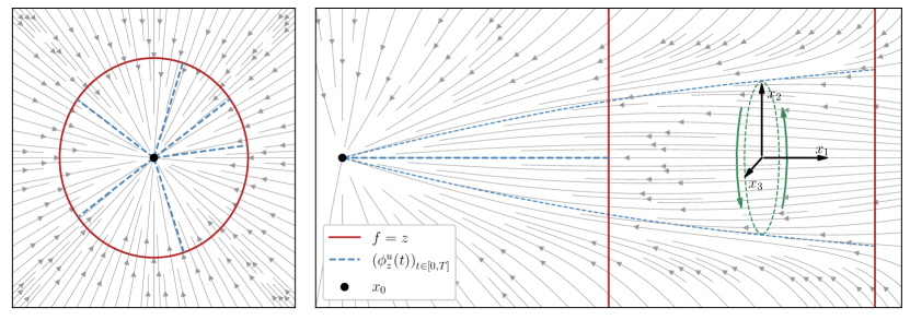
Figure 1: Left: Example for the simplest scenario where the instanton has to break the symmetry of the system including the observable at any $z$ or $\lambda$. Here, $b$ is a radial vector field and $f(x)=\norm{x}_{n}$. An example of this kind is discussed in Section 4.1. Right: Example for a problem with spontaneous symmetry breaking. Suppose that the whole system is three-dimensional, such that the plot only shows the $(x_{1},x_{2})$-plane at $x_{3}=0$, and that the system is rotationally symmetric about the $x_{1}$ axis. Then, the instanton realizing a given value of $z=x_{1}$ at the final time, as indicated by the red planes, could, for a suitably constructed drift, break its symmetry beyond a critical value $z_{c}$, thereby transitioning from a solution with $(x_{2},x_{3})=0$ along the whole path to a continuous family of instantons, indicated by the green arrows symbolizing out of plane rotation. A toy example for such an instance of spontaneous symmetry breaking is considered in Section 4.3.

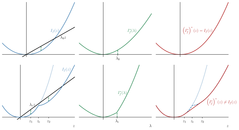
Figure 2: Top row: The simplest scenario where the rate function $I_{f}$ is strictly convex, its Legendre-Fenchel dual $I^{*}_{f}$ (that is computed by minimizing the augmented action functional at fixed $\lambda$) is finite and differentiable everywhere, and transforming from the MGF to the PDF via a saddlepoint approximation yields the original rate function. Note that this situation can still occur if there are zero modes present in the computation of the prefactor of the MGF $A_{f}^{\varepsilon}$. Bottom row: A different rate function where at a critical observable value $z_{\text{c}}$, the instanton solution spontaneously breaks some of its symmetries in order to realize a given observable value with less action cost than on the symmetric, dotted branch. In the specific case of a first order phase transition as sketched here, the rate function is no longer convex, its dual is non-differentiable at a critical $\lambda_{\text{c}}$, and transforming from the MGF to the PDF yields the convex hull of the original rate function.

In order to derive appropriately modified prefactor formulas, we will use the following, conceptually simple strategy: First, we split the integration in path space into components along the submanifold of degenerate minimizers and the subspace which is $L^{2}$-orthogonal to it. For each point on the submanifold, we can then use Laplace’s method on the normal space, where all flat directions of the second variation of the action are removed by construction. Then, a boundary-type regularization procedure McKane and Tarlie (1995); Kleinert and Chervyakov (1998); Falco et al. (2017) is used to compute functional determinants with removed zero eigenvalues by integrating a Riccati equation similar to the non-degenerate case.

We start with a brief motivation in finitely many dimensions, as well as two simple examples: Consider the Laplace-type integral

$$J_{\varepsilon}=\int_{\mathds{R}^{n}}h(x)e^{-S(x)/\varepsilon}\differential^{n}x\,,$$ (96)

in the case where there is a family of global minimizers ${\cal M}^{r}$ of $S:\mathds{R}^{n}\to\mathds{R}$, and $h:\mathds{R}^{n}\to\mathds{R}$ is any continuous function. We assume that ${\cal M}^{r}=\operatorname*{arg\,min}S$ is an $r$-dimensional submanifold of $\mathds{R}^{n}$ with $0<r<n$. Then, we know that for small $\varepsilon>0$, the integral $J_{\varepsilon}$ is dominated by the behavior of $S$ in an open neighborhood $U_{{\cal M}^{r}}$ of ${\cal M}^{r}$, such that

$$J_{\varepsilon}\overset{\varepsilon\downarrow 0}{\sim}\int_{U_{{\cal M}^{r}}}h(x)e^{-S(x)/\varepsilon}\differential^{n}x\overset{\varepsilon\downarrow 0}{\sim}\int_{{\cal M}^{r}}\differential^{r}\mu(y)\int_{N_{y}{\cal M}^{r}}\differential^{n-r}z\ h(y+z)e^{-S(y+z)/\varepsilon}\,,$$ (97)

where the integration was split into the integration along ${\cal M}^{r}$ (with surface measure $\differential^{r}\mu$) and the (entire, for $\varepsilon\downarrow 0$) normal space $N_{y}{\cal M}^{r}$ perpendicular to the hypersurface ${\cal M}^{r}$. This split of integration directions is usually done formally using the Faddeev-Popov method Faddeev and Popov (1967) in the physics literature, which consists of inserting a suitable Dirac $\delta$ function into the initial integral. For each $y\in{\cal M}^{r}$, applying Laplace’s method in $z$ yields

$$J_{\varepsilon}\overset{\varepsilon\downarrow 0}{\sim} (2\pi\varepsilon)^{(n-r)/2}\int_{{\cal M}^{r}}\differential^{r}\mu(y)\frac{h(y)e^{-S(y)/\varepsilon}}{\sqrt{{\det}^{\prime}_{n-r}(\nabla^{2}S(y))}}$$

$$= (2\pi\varepsilon)^{(n-r)/2}e^{-S(y_{0})/\varepsilon}\int_{{\cal M}^{r}}\differential^{r}\mu(y)\frac{h(y)}{\sqrt{{\det}^{\prime}_{n-r}(\nabla^{2}S(y))}}\,,$$ (98)

where ${\det}^{\prime}_{n-r}$ denotes the removal of the $r$ zero eigenvalues of the matrix $\nabla^{2}S(y)\in\mathds{R}^{n\times n}$ from the determinant that correspond to eigenvectors in the tangent space $T_{y}{\cal M}^{r}$. In the second line, we used that $S$ is constant in ${\cal M}^{r}$ in order to pull the exponential factor out of the integral, evaluated at any $y_{0}\in{\cal M}^{r}$. Now, there are two cases: If ${\det}^{\prime}_{n-r}(\nabla^{2}S)$ and $h$ are constant along ${\cal M}^{r}$, the volume of ${\cal M}^{r}$ factors out and we obtain (if this volume is finite; otherwise, the integral is infinite and needs to be regularized in some way in order to make sense of it, e.g. by normalizing it with respect to the volume)

$$J_{\varepsilon}\overset{\varepsilon\downarrow 0}{\sim} (2\pi\varepsilon)^{(n-r)/2}\operatorname{vol}\left({\cal M}^{r}\right)\frac{h(y_{0})e^{-S(y_{0})/\varepsilon}}{\sqrt{{\det}^{\prime}_{n-r}(\nabla^{2}S(y_{0}))}}\,.$$ (99)

Otherwise, the integral along ${\cal M}^{r}$ in (98) needs to be evaluated explicitly. It is easy to find two-dimensional examples ($n=2$, $r=1$) for either case (with $h\equiv 1$):

1. Consider $S:\mathds{R}^{2}\to\mathds{R}$, $S(x,y)=(1+x^{4})y^{2}$. Then the set of minimizers of $S$ is given by the $(r=1)$-dimensional manifold ${\cal M}^{1}=\left\{(x,0)\in\mathds{R}^{2}\right\}$ with $S|_{{\cal M}^{1}}=0$, and Hessian $\nabla^{2}S(x,0)=\text{diag}(0,2(1+x^{4}))$. Since the integration along $y$ for each $x$ is already Gaussian, (98) yields the exact result

   $$J_{\varepsilon}=(2\pi\varepsilon)^{1/2}\int_{-\infty}^{\infty}\frac{\differential x}{\sqrt{{\det}^{\prime}_{1}(\nabla S(x,0))}}=\left(\pi\varepsilon\right)^{1/2}\int_{-\infty}^{\infty}\frac{\differential x}{\sqrt{1+x^{4}}}=\frac{\Gamma\left(\frac{1}{4}\right)^{2}}{2}\sqrt{\varepsilon}\,.$$ (100)

   Notably, in this case, ${\det}^{\prime}_{n-r}(\nabla^{2}S)$ is not constant along the family of minimizers, and the dependency of $\nabla^{2}S$ on $x$ was needed in order to obtain the correct, finite result despite the infinite volume of the family of minimizers. Also, in this example, while the action on ${\cal M}^{1}$ is constant (and equal to 0) under translations $x\to x+\delta x$, this is not true for the action $S$ on all of $\mathds{R}^{2}$.

2. Next, consider $S:\mathds{R}^{2}\to\mathds{R}$, $S(x,y)=\left(x^{2}+y^{2}-a^{2}\right)^{2}$ with $a>0$, such that the set of minimizers is the $r=1$-dimensional manifold ${\cal M}^{1}=\left\{(x,y)\in\mathds{R}^{2}\mid x^{2}+y^{2}=a^{2}\right\}$. Here, the eigenvalues of the Hessian at the minimizers are given by $\lambda_{0}=0$ and $\lambda_{1}=8a^{2}$. In this case, the eigenvalues are independent of the position on ${\cal M}^{1}$, since the entire action is rotationally invariant. From (99), we obtain $J_{\varepsilon}\overset{\varepsilon\downarrow 0}{\sim}(2\pi\varepsilon)^{1/2}2\pi a(8a^{2})^{-1/2}=\pi^{3/2}\varepsilon^{1/2}\,,$ in accordance with the $\varepsilon\downarrow 0$ asymptotics of the exact result $J_{\varepsilon}=\pi^{3/2}\varepsilon^{1/2}\left[1+\erf\left(a^{2}/\varepsilon\right)\right]/2$.

3.2 Moment-generating function prefactor estimates for Freidlin-Wentzell theory with zero modes

In our setup of sample path large deviation theory, we will only consider the second scenario where the volume of the manifold factors out and is finite. Note that in this sense, the volume part in the prefactor can always be trivially found, such as a sphere or box volume of the “equi-observable” hypersurfaces, and the nontrivial part of our analysis is to find the exact way in which the Riccati approach can be adjusted when the second variation functional possesses vanishing eigenvalues.

Usually, when solving the instanton equations (5) for $(\phi_{\lambda},\theta_{\lambda})$ in the situation that there is an $r$-dimensional submanifold, $r\geq 1$, of global minimizers ${\cal M}^{r}_{\lambda}$, we will find a specific parameterization of ${\cal M}^{r}_{\lambda}$, $u\mapsto\phi_{\lambda}^{u}$ for $u\in D\subseteq\mathds{R}^{r}$. Then, a basis of the tangent space $T_{\phi_{\lambda}^{u}}{\cal M}^{r}_{\lambda}$ is given by the zero modes

$$\psi^{u}_{\lambda,i}:=\partialderivative{\phi_{\lambda}^{u}}{u_{i}}:[0,T]\to\mathds{R}^{n}$$ (101)

with $i=1,\dots,r$. We denote the corresponding momentum fluctuations as

$$\xi^{u}_{\lambda,i}:=\partialderivative{\theta_{\lambda}^{u}}{u_{i}}=a^{-1}\left[\derivative{t}-\nabla b(\phi_{\lambda}^{u})-\left(\nabla a(\phi_{\lambda}^{u})\theta_{\lambda}^{u}\right)\right]\psi^{u}_{\lambda,i}\,.$$ (102)

We make the following two observations:

• The zero modes $\psi^{u}_{\lambda,i}$, $i=1,\dots,r$ satisfy the Jacobi equation (36) (or, equivalently, (43)), since

  $$\left.\functionalderivative{S}{\phi}\right|_{\phi_{\lambda}^{u}}=0\;\forall u\in D\quad\overset{\partial/\partial u_{i}}{\Rightarrow}\quad\left.\functionalderivative[2]{S}{\phi}\right|_{\phi_{\lambda}^{u}}\psi^{u}_{\lambda,i}=\Omega[\phi_{\lambda}^{u}]\psi^{u}_{\lambda,i}=0\;\forall u\in D\,,$$ (103)

  as well as the boundary conditions ${\cal A}_{\lambda}^{u}$ of the second variation, because

  $$\phi^{u}_{\lambda}(0)=x\;\forall u\in D\quad\overset{\partial/\partial u_{i}}{\Rightarrow}\quad\psi^{u}_{\lambda,i}(0)=0$$

  $$\theta_{\lambda}^{u}(T)=\lambda\nabla f(\phi_{\lambda}^{u}(T))\quad\overset{\partial/\partial u_{i}}{\Rightarrow}\quad\xi^{u}_{\lambda,i}(T)=\lambda\nabla^{2}f(\phi_{\lambda}^{u}(T))\psi^{u}_{\lambda,i}(T)\,.$$ (104)

  Hence, each of the zero modes is an admissible eigenfunction of the Jacobi operator $\Omega[\phi_{\lambda}^{u}]$ under ${\cal A}_{\lambda}^{u}$ with eigenvalue $\lambda^{(0)}_{i}=0$ and it follows that $\operatorname{Det}_{{\cal A}_{\lambda}}\left(\Omega[\phi_{\lambda}^{u}]\right)=0$.

• We can immediately conclude that $r\leq n$ since there are at most $n$ linearly independent solutions of the first order Jacobi equation (36), i.e.

  $$\derivative{t}\left(\begin{array}[]{c}\gamma\\ \zeta\end{array}\right)=\Gamma\left[\phi_{\lambda}^{u}\right]\left(\begin{array}[]{c}\gamma\\ \zeta\end{array}\right)$$ (109)

  that satisfy the initial condition $\gamma(0)=0\in\mathds{R}^{n}$.

It is now straightforward to formulate the analogue of Proposition 2.2 in the presence of zero modes:

[Sharp estimates for MGFs via functional determinants in case of broken symmetries] Denote by $\phi_{\lambda}^{u}\in{\cal M}^{r}_{\lambda}$, parameterized by $u\in D\subset\mathds{R}^{r}$, the elements of the $r$-dimensional submanifold of instanton solutions of the minimization problem

$$\inf_{\phi(0)=x}\left(S[\phi]-\lambda f(\phi(T))\right)$$ (110)

and by $\phi_{0}$ the unique “free” instanton, solution to the minimization problems

$$\inf_{\phi(0)=x}S[\phi]$$ (111)

for the Freidlin-Wentzell action (3). Further, for variations $\gamma:[0,T]\to\mathds{R}^{n}$, let

$$\delta^{2}S[\phi][\gamma] =\frac{1}{2}\int_{0}^{T}\left\langle\gamma,\Omega[\phi]\gamma\right\rangle_{n}\differential t$$ (112)

be the second variation of $S$ around $\phi$, where the linear operator $\Omega$ is given by (10) and we impose mixed Dirichlet-Robin boundary conditions ${\cal A}_{\lambda}^{u_{0}}$, defined in (11), along $\phi=\phi_{\lambda}^{u_{0}}$ for any $u_{0}\in D$. Then we have the following sharp asymptotic estimate for the MGF $A_{f}^{\varepsilon}$:

$$A_{f}^{\varepsilon}(\lambda)\overset{\varepsilon\downarrow 0}{\sim}(2\pi\varepsilon)^{-r/2}\tilde{R}_{\lambda}\exp\left\{-\varepsilon^{-1}\left(S[\phi_{\lambda}^{u_{0}}]-\lambda f\left(\phi_{\lambda}^{u_{0}}(T)\right)\right)\right\}$$ (113)

with

$$\tilde{R}_{\lambda}:= \operatorname{vol}\left({\cal M}^{r}_{\lambda}\right)\left(\frac{\operatorname{Det}^{\prime}_{{\cal A}_{\lambda}^{u_{0}}}\left(a(\phi_{\lambda}^{u_{0}})\Omega[\phi_{\lambda}^{u_{0}}]\right)}{\operatorname{Det}_{{\cal A}_{0}}\left(a(\phi_{0})\Omega[\phi_{0}]\right)}\right)^{-1/2}\times$$

$$\hskip 56.9055pt\times\exp\left\{-\tfrac{1}{2}\int_{0}^{T}\left(\nabla\cdot b(\phi_{\lambda}^{u_{0}})+\tr\left[\nabla a(\phi_{\lambda}^{u_{0}})\theta_{\lambda}^{u_{0}}\right]-\nabla\cdot b(\phi_{0})\right)\,\differential t\right\}\,.$$ (114)

Here, $\operatorname{Det}^{\prime}$ denotes the functional determinant after removal of all $r$ zero eigenvalues.

For the given parameterization $u\mapsto\phi_{\lambda}^{u}$, the volume of ${\cal M}^{r}_{\lambda}$ can be computed as

$$\operatorname{vol}\left({\cal M}^{r}_{\lambda}\right)=\int_{D}\sqrt{{\det}_{r}\left\llangle\psi^{u}_{\lambda}\middle|\psi^{u}_{\lambda}\right\rrangle}\;\differential^{r}u\,$$

where $\left\llangle\psi^{u}_{\lambda}\middle|\psi^{u}_{\lambda}\right\rrangle\in\mathds{R}^{r\times r}$ is the Gram matrix defined via

$$\left\llangle\psi^{u}_{\lambda}\middle|\psi^{u}_{\lambda}\right\rrangle_{ij}:=\left\langle\psi^{u}_{\lambda,i},\psi^{u}_{\lambda,j}\right\rangle_{L^{2}([0,T],\mathds{R}^{n})}\,.$$ (115)

In order to be able to compute the ratio

$$\frac{\operatorname{Det}^{\prime}_{{\cal A}_{\lambda}^{u_{0}}}\left(a(\phi_{\lambda}^{u_{0}})\Omega[\phi_{\lambda}^{u_{0}}]\right)}{\operatorname{Det}_{{\cal A}_{0}}\left(a(\phi_{0})\Omega[\phi_{0}]\right)}$$ (116)

in $\tilde{R}_{\lambda}$ efficiently using Forman’s theorem, without having to compute and multiply all non-zero eigenvalues of both operators, we use a technique based on boundary perturbations. The concept of the following treatment is described in Falco et al. (2017), who discuss the case of an arbitrary number of zero modes with Dirichlet and (anti)-periodic boundary conditions. A related paper in this regard is also Corazza and Singh (2022). Note, however, that these references do not derive manifestly parameterization-invariant results, and further discuss neither the boundary conditions specific for low dimensional observables in sample path large deviations, nor the relation to efficient numerical prefactor computations using Riccati equations.

The idea of the boundary regularization procedure to compute $\operatorname{Det}_{{\cal A}_{\lambda}^{u_{0}}}^{\prime}\left(a(\phi_{\lambda}^{u_{0}})\Omega[\phi_{\lambda}^{u_{0}}]\right)$ is as follows: We modify the boundary conditions ${\cal A}_{\lambda}^{u_{0}}$, realized through $M_{\lambda}^{u_{0}},N_{\lambda}^{u_{0}}\in\mathds{R}^{2n\times 2n}$, using a small perturbation, that is, we replace them by $M_{\lambda}^{u_{0}}(\delta),N_{\lambda}^{u_{0}}(\delta)\in\mathds{R}^{2n\times 2n}$ with $\delta=(\delta_{1},\dots,\delta_{r})\in\mathds{R}^{r}$, such that $M_{\lambda}^{u_{0}}(0)=M_{\lambda}^{u_{0}}$ and $N_{\lambda}^{u_{0}}(0)=N_{\lambda}^{u_{0}}$. The boundary perturbation has to be chosen in such a way as to remove all zero eigenvalues of $\Omega[\phi_{\lambda}^{u_{0}}]$. Then we carry out the following three steps:

1. Explicitly compute the leading order asymptotics of the $r$ nonzero eigenvalues $\lambda_{1}^{(0)}(\delta),\dots,\lambda_{r}^{(0)}(\delta)$ of $\Omega[\phi_{\lambda}^{u_{0}}]$ under $M_{\lambda}^{u_{0}}(\delta),N_{\lambda}^{u_{0}}(\delta)$ that tend to 0 as $\delta\to 0$.

2. Apply Forman’s theorem to evaluate the full, nonzero determinant $\operatorname{Det}_{{\cal A}_{\lambda}^{u_{0}}(\delta)}\left(a(\phi_{\lambda}^{u_{0}})\Omega[\phi_{\lambda}^{u_{0}}]\right)$.

3. Evaluate

   $$\operatorname{Det}_{{\cal A}_{\lambda}^{u_{0}}}^{\prime}\left(a(\phi_{\lambda}^{u_{0}})\Omega[\phi_{\lambda}^{u_{0}}]\right)\overset{\cdot}{=}\lim_{\delta\to 0}\left[\frac{\operatorname{Det}_{{\cal A}_{\lambda}^{u_{0}}(\delta)}\left(a(\phi_{\lambda}^{u_{0}})\Omega[\phi_{\lambda}^{u_{0}}]\right)}{\prod_{i=1}^{r}\lambda_{i}^{(0)}(\delta)}\right]\,.$$ (117)

Of course, step 2 and 3 only make sense when considering ratios of functional determinants; however, since it is irrelevant to the following discussion, we omit the division by the free determinant for the time being and denote equalities up to division by the free determinant via “$\overset{\cdot}{=}$” as in Falco et al. (2017).

In our setup, there are different types of regularization that can be chosen depending on the assumptions. We start with the case of a nonlinear observable with positive definite matrix

$$\bra{\psi^{u}_{\lambda}(T)}\nabla^{2}f(\phi^{u}_{\lambda}(T))\ket{\psi^{u}_{\lambda}(T)}\in\mathds{R}^{r\times r}\,,$$ (118)

where

$$\bra{\psi^{u}_{\lambda}(T)}\nabla^{2}f(\phi^{u}_{\lambda}(T))\ket{\psi^{u}(T)}_{ij}=\left\langle\psi^{u}_{\lambda,i}(T),\nabla^{2}f(\phi^{u}_{\lambda}(T))\psi^{u}_{\lambda,j}(T)\right\rangle_{n}\,.$$ (119)

Importantly, the zero modes $(\psi^{u},\xi^{u})$ are, due to their initial conditions $\psi^{u}(0)=0$ and $\xi^{u}(0)\neq 0$, part of the $n$ solutions $(\gamma,\zeta)$ that make up the forward Riccati matrix solution with $Q=\gamma\zeta^{-1}$ and $Q(0)=0$. Now, since $\nabla^{2}f(\phi^{u}_{\lambda}(T))$ is non-degenerate on the space of final time zero mode states $\psi^{u}(T)$, we conclude that $\xi^{u}(T)$ will also be nondegenerate due to the boundary conditions of the zero modes. Hence, the forward Riccati differential equation for $Q$ remains well-posed and $Q(t)$ does not explode as $t\to T$, the only problem being the removal of zero eigenvalues of ${\det}_{n}\left(1_{n\times n}-\lambda\nabla^{2}f\left(\phi_{\lambda}(T)\right)Q_{\lambda}(T)\right)$ in Proposition 2.2.

In this case, the problem can be regularized using the perturbation

$$N_{\lambda}^{u_{0}}=\left(\begin{array}[]{c|c}0_{n\times n}&0_{n\times n}\\ \hline\cr-\lambda\nabla^{2}f(\phi_{\lambda}^{u}(T))&1_{n\times n}\end{array}\right)\rightarrow N_{\lambda}^{u_{0}}(\delta):=\left(\begin{array}[]{c|c}0_{n\times n}&0_{n\times n}\\ \hline\cr-\lambda\nabla^{2}f(\phi_{\lambda}^{u}(T))&1_{n\times n}+\sum_{i=1}^{r}\delta_{i}\cdot\tilde{\xi}^{u_{0}}_{\lambda,i}\otimes\tilde{\xi}^{u_{0}}_{\lambda,i}\end{array}\right)$$ (124)

where $\left\{\tilde{\xi}^{u_{0}}_{\lambda,1},\dots,\tilde{\xi}^{u_{0}}_{\lambda,r}\right\}$ is any (oriented) orthonormal basis of the vector space $\text{span}\left\{\xi^{u_{0}}_{\lambda,1}(T),\dots,\xi^{u_{0}}_{\lambda,1}(T)\right\}\subset\mathds{R}^{n}$ spanned by the zero mode momenta at $t=T$. Let us denote by $\psi^{u_{0}}_{\lambda,i}(\delta)$ the eigenfunctions of $\Omega[\phi_{\lambda}^{u_{0}}]$ under these boundary conditions ${\cal A}_{\lambda}^{u_{0}}(\delta)$ that tend to the zero modes $\psi^{u}_{\lambda,i}$ as $\delta\to 0$. Then we have the following leading order asymptotics of $\prod_{i=1}^{r}\lambda_{i}^{(0)}(\delta)$ for step 1 with this particular regularization:

[Leading order behavior of the quasi-zero eigenvalues] For the boundary regularization (124), the asymptotic behavior of the regularized zero eigenvalues of $\Omega[\phi_{\lambda}^{u_{0}}]$ is

$$\prod_{i=1}^{r}\lambda^{(0)}_{i}(\delta)\overset{\delta\to 0}{\sim}\frac{{\det}_{r}\bra{\psi^{u_{0}}_{\lambda}(T)}\lambda\nabla^{2}f(\phi^{u_{0}}_{\lambda}(T))\ket{\psi^{u_{0}}_{\lambda}(T)}}{{\det}_{r}\left\llangle\psi^{u_{0}}_{\lambda}\middle|\psi^{u_{0}}_{\lambda}\right\rrangle}\prod_{i=1}^{r}\delta_{i}\,.$$ (125)

Derivation of Lemma 3.2 :

The modified boundary conditions at $t=T$ read

$$\left\langle\zeta(T)-\lambda\nabla^{2}f(\phi_{\lambda}^{u}(T))\gamma(T),\tilde{\xi}^{u_{0}}_{\lambda,i}\right\rangle_{n}=-\delta_{i}\left\langle\zeta(T),\tilde{\xi}^{u_{0}}_{\lambda,i}\right\rangle_{n}\,,\quad i=1,\dots,r\,.$$ (126)

For any $i,j\in\left\{1,\dots,r\right\}$, we compute

$$\left\langle\psi^{u_{0}}_{\lambda,i},\Omega[\phi_{\lambda}^{u_{0}}]\psi^{u_{0}}_{\lambda,j}(\delta)\right\rangle_{L^{2}([0,T],\mathds{R}^{n})}\overset{\text{eigenvalue}}{=}\lambda^{(0)}_{j}(\delta)\left\langle\psi^{u_{0}}_{\lambda,i},\psi^{u_{0}}_{\lambda,j}(\delta)\right\rangle_{L^{2}([0,T],\mathds{R}^{n})}$$

$$\overset{\text{adjoining }\Omega}{=}\left.\left\langle\xi^{u_{0}}_{\lambda,i},\psi^{u_{0}}_{\lambda,j}(\delta)\right\rangle_{n}\right|^{T}_{0}-\left.\left\langle\psi^{u_{0}}_{\lambda,i},\xi^{u_{0}}_{\lambda,j}(\delta)\right\rangle_{n}\right|^{T}_{0}+\underbrace{\left\langle\Omega[\phi_{\lambda}^{u_{0}}]\psi^{u_{0}}_{\lambda,i},\psi^{u_{0}}_{\lambda,j}(\delta)\right\rangle_{L^{2}([0,T],\mathds{R}^{n})}}_{=0}$$

$$\overset{\text{boundary conditions}}{=}-\left\langle\psi^{u_{0}}_{\lambda,i}(T),\xi^{u_{0}}_{\lambda,j}(\delta)(T)-\lambda\nabla^{2}f(\phi^{u_{0}}_{\lambda}(T))\psi^{u_{0}}_{\lambda,j}(\delta)(T)\right\rangle_{n}$$

$$=-\sum_{k=1}^{r}\left\langle\psi^{u_{0}}_{\lambda,i}(T),\tilde{\xi}^{u_{0}}_{\lambda,k}\right\rangle_{n}\underbrace{\left\langle\tilde{\xi}^{u_{0}}_{\lambda,k},\xi^{u_{0}}_{\lambda,j}(\delta)(T)-\lambda\nabla^{2}f(\phi^{u_{0}}_{\lambda}(T))\psi^{u_{0}}_{\lambda,j}(\delta)(T)\right\rangle_{n}}_{=-\delta_{k}\left\langle\tilde{\xi}^{u_{0}}_{\lambda,k},\xi^{u_{0}}_{\lambda,j}(\delta)(T)\right\rangle_{n}}$$

$$=\left(\bra{\psi^{u_{0}}_{\lambda}(T)}\ket{\tilde{\xi}^{u_{0}}_{\lambda}}\text{diag}_{r}(\delta)\bra{\tilde{\xi}^{u_{0}}_{\lambda}}\ket{\xi^{u_{0}}_{\lambda}(\delta)(T)}\right)_{ij}$$

$$\overset{\text{cf.\ first line}}{=}\left(\left\llangle\psi^{u_{0}}_{\lambda}\middle|\psi^{u_{0}}_{\lambda}(\delta)\right\rrangle\text{diag}_{r}(\lambda^{(0)}(\delta))\right)_{ij}\,.$$ (127)

Computing the determinant of these expressions yields

$$\prod_{i=1}^{r}\lambda^{(0)}_{i}(\delta)=\frac{{\det}_{r}\bra{\psi^{u_{0}}_{\lambda}(T)}\ket{\xi^{u_{0}}_{\lambda}(\delta)(T)}}{{\det}_{r}\left\llangle\psi^{u_{0}}_{\lambda}\middle|\psi^{u_{0}}_{\lambda}(\delta)\right\rrangle}\prod_{i=1}^{r}\delta_{i}\overset{\delta\to 0}{\sim}\frac{{\det}_{r}\bra{\psi^{u_{0}}_{\lambda}(T)}\ket{\xi^{u_{0}}_{\lambda}(T)}}{{\det}_{r}\left\llangle\psi^{u_{0}}_{\lambda}\middle|\psi^{u_{0}}_{\lambda}\right\rrangle}\prod_{i=1}^{r}\delta_{i}\,.$$ (128)

In the last step, note that it will not be true in general that $\psi^{u_{0}}_{\lambda,i}(\delta)\to\psi^{u_{0}}_{\lambda,i}$ as $\delta\to 0$ for each $i=1,\dots,r$ individually (cf. Falco et al. (2017)), but due to linearity, the transformation matrices from $\lim_{\delta\to 0}\psi^{u_{0}}_{\lambda}(\delta)$ to $\psi^{u_{0}}_{\lambda}$ and from $\lim_{\delta\to 0}\xi^{u_{0}}_{\lambda}(\delta)$ to $\xi^{u_{0}}_{\lambda}$ will coincide and their determinants therefore cancel in the last step. $\square$

[Forman’s theorem for the perturbed boundary conditions] For the boundary regularization (124) and any $\delta\in\mathds{R}^{r}$, the functional determinant of $\Omega[\phi_{z}^{u_{0}}]$ under ${\cal A}_{z}^{u_{0}}(\delta)$ can be expressed as

$$\operatorname{Det}_{{\cal A}_{\lambda}^{u_{0}}(\delta)}\left(a(\phi_{\lambda}^{u_{0}})\Omega[\phi_{\lambda}^{u_{0}}]\right) \overset{\cdot}{=}{\det}_{n-r}^{\prime}\left(\zeta(T)-\lambda\nabla^{2}f(\phi^{u_{0}}_{\lambda}(T)\gamma(T)\right)\times$$

$$\hskip 85.35826pt\times\frac{\sqrt{{\det}_{r}\bra{\xi^{u_{0}}_{\lambda}(T)}\ket{\xi^{u_{0}}_{\lambda}(T)}}}{{\det}_{r}\left(\bra{\tilde{\xi}^{u_{0}}_{\lambda}}\ket{\xi^{u_{0}}_{\lambda}(0)}\right)}\cdot\left(\prod_{i=1}^{r}\delta_{i}\right)\,,$$ (129)

where $(\gamma,\zeta):[0,T]\to\mathds{R}^{2n\times n}$ is the solution of

$$\derivative{t}\left(\begin{array}[]{c}\gamma\\ \zeta\end{array}\right)=\Gamma\left[\phi_{\lambda}^{u_{0}}\right]\left(\begin{array}[]{c}\gamma\\ \zeta\end{array}\right)\,,\quad\left(\begin{array}[]{c}\gamma(0)\\ \zeta(0)\end{array}\right)=\left(\begin{array}[]{c}0_{n\times n}\\ \left(\xi^{u_{0}}_{\lambda,1}(0),\dots,\xi^{u_{0}}_{\lambda,r}(0),v_{1},\dots,v_{n-r}\right)\end{array}\right)\,.$$ (138)

Derivation of Lemma 3.2 :

We pick an orthonormal basis of $\mathds{R}^{n}$ by extending $\left\{\tilde{\xi}^{u_{0}}_{\lambda,1},\dots,\tilde{\xi}^{u_{0}}_{\lambda,r}\right\}$ by $n-r$ additional unit vectors $v_{1},\dots,v_{n-r}$. In this basis, the right boundary matrix $N_{\lambda}^{u_{0}}(\delta)$ from (124) becomes

$$N_{\lambda}^{u_{0}}(\delta):=\left(\begin{array}[]{c|c}0_{n\times n}&0_{n\times n}\\ \hline\cr-\lambda\nabla^{2}f(\phi_{\lambda}^{u}(T))&\begin{array}[]{c|c}1_{r\times r}+\text{diag}_{r}\left(\delta\right)&0_{r\times(n-r)}\\ \hline\cr 0_{(n-r)\times r}&1_{(n-r)\times(n-r)}\end{array}\end{array}\right)\,.$$ (143)

For the fundamental system of solutions $\Upsilon$, we choose the initial condition

$$\Upsilon(0)=\left(\begin{array}[]{c|c}1_{n\times n}&0_{n\times n}\\ \hline\cr 0_{n\times n}&\begin{array}[]{c|c}\bra{\tilde{\xi}^{u_{0}}_{\lambda}}\ket{\xi^{u_{0}}_{\lambda}(t=0)}&0_{r\times(n-r)}\\ \hline\cr\bra{v}\ket{\xi^{u_{0}}_{\lambda}(t=0)}&1_{(n-r)\times(n-r)}\end{array}\end{array}\right)$$ (148)

such that

$${\det}_{2n}\Upsilon(0)={\det}_{n}\zeta(0)={\det}_{n}\left(\xi^{u_{0}}_{\lambda,1}(0),\dots,\xi^{u_{0}}_{\lambda,r}(0),v_{1},\dots,v_{n-r}\right)={\det}_{r}\left(\bra{\tilde{\xi}^{u_{0}}_{\lambda}}\ket{\xi^{u_{0}}_{\lambda}(t=0)}\right)$$ (149)

and

$${\det}_{2n}\left(M^{u_{0}}_{\lambda}\Upsilon(0)+N^{u_{0}}_{\lambda}(\delta)\Upsilon(T)\right)$$

$$={\det}_{2n}\left(\begin{array}[]{c|c}1_{n\times n}&0_{n\times n}\\ \hline\cr(*)_{n\times n}&\begin{array}[]{c|c}\text{diag}_{r}\left(\delta\right)\bra{\tilde{\xi}^{u_{0}}_{\lambda}}\ket{\xi^{u_{0}}_{\lambda}(t=T)}&(*)_{r\times(n-r)}\\ \hline\cr 0_{(n-r)\times r}&\left[\zeta(T)-\lambda\nabla^{2}(\phi^{u_{0}}_{\lambda}(T))\gamma(T)\right]_{\perp}\end{array}\end{array}\right)$$ (154)

$$=\left(\prod_{i=1}^{r}\delta i\right)\sqrt{{\det}_{r}\bra{\xi^{u_{0}}_{z}(t=T)}\ket{\xi^{u_{0}}_{z}(t=T)}}{\det}_{n-r}^{\prime}\left(\zeta(T)-\lambda\nabla^{2}f(\phi^{u_{0}}_{\lambda}(T)\gamma(T)\right)\,.$$ (155)

$\square$

Combining the previous two lemmas with Proposition 3.2 and observing that for the solutions $(\gamma,\zeta)$ of the Jacobi equation in Lemma 3.2, we have

$${\det}_{n-r}^{\prime}\left(\zeta(T)-\lambda\nabla^{2}f(\phi^{u_{0}}_{\lambda}(T))\gamma(T)\right)={\det}_{n-r}^{\prime}\left(1_{n\times n}-\lambda\nabla^{2}f(\phi^{u_{0}}_{\lambda}(T))Q(T)\right)\frac{\det_{n}\zeta(T)}{\sqrt{{\det}_{r}\bra{\xi^{u_{0}}_{\lambda}(T)}\ket{\xi^{u_{0}}_{\lambda}(T)}}}\,,$$ (156)

which yields the following concrete formula to evaluate the MGF prefactor in the presence of zero modes for nondegenerate, nonlinear observables:

[MGF prefactor with zero modes via forward Riccati equation for nondegenerate, nonlinear observables] The prefactor $\tilde{R}_{\lambda}$ in (114) can be computed as

$$\tilde{R}_{\lambda} =\frac{\exp\left\{\frac{1}{2}\int_{0}^{T}\tr\left[\left(\left\langle\nabla^{2}b(\phi_{\lambda}^{u_{0}}),\theta_{\lambda}^{u_{0}}\right\rangle_{n}+\tfrac{1}{2}\left\langle\theta_{\lambda}^{u_{0}},\nabla^{2}a(\phi_{\lambda}^{u_{0}})\theta_{\lambda}^{u_{0}}\right\rangle_{n}\right)Q_{\lambda}^{u_{0}}\right]\differential t\right\}}{\left[{\det}_{n-r}^{\prime}\left(1_{n\times n}-\lambda\nabla^{2}f(\phi^{u_{0}}_{\lambda}(T))Q^{u_{0}}_{\lambda}(T)\right)\right]^{1/2}}\times$$

$$\hskip 56.9055pt\times\int_{D}\sqrt{{\det}_{r}\bra{\psi^{u}_{\lambda}(T)}\lambda\nabla^{2}f(\phi^{u}_{\lambda}(T))\ket{\psi^{u}_{\lambda}(T)}}\;\differential^{r}u$$ (157)

for any $u_{0}\in\mathds{R}^{r}$, where $Q^{u_{0}}_{\lambda}:[0,T]\to\mathds{R}^{n\times n}$ solves the forward Riccati equation

$$\begin{cases}\dot{Q}_{\lambda}^{u_{0}}=a(\phi_{\lambda}^{u_{0}})+Q_{\lambda}^{u_{0}}\left[\nabla b\left(\phi_{\lambda}^{u_{0}}\right)^{\top}+\left(\nabla a(\phi_{\lambda}^{u_{0}})\theta_{\lambda}^{u_{0}}\right)^{\top}\right]\\ \quad+\left[\nabla b\left(\phi_{\lambda}^{u_{0}}\right)+\left(\nabla a(\phi_{\lambda}^{u_{0}})\theta_{\lambda}^{u_{0}}\right)\right]Q_{\lambda}^{u_{0}}+Q_{\lambda}^{u_{0}}\left[\left<\nabla^{2}b(\phi_{\lambda}^{u_{0}}),\theta_{\lambda}^{u_{0}}\right>_{n}+\tfrac{1}{2}\left\langle\theta_{\lambda}^{u_{0}},\nabla^{2}a(\phi_{\lambda}^{u_{0}})\theta_{\lambda}^{u_{0}}\right\rangle_{n}\right]Q_{\lambda}^{u_{0}}\,,\\ Q_{\lambda}^{u_{0}}(0)=0_{n\times n}\in\mathds{R}^{n\times n}\,.\end{cases}$$ (158)

The second case that we consider is when the matrix

$$\bra{\psi^{u}_{\lambda}(T)}\nabla^{2}f(\phi^{u}_{\lambda}(T))\ket{\psi^{u}_{\lambda}(T)}\in\mathds{R}^{r\times r}$$ (159)

is not positive definite, which is in particular relevant for the important case of linear observables. Here, the regularization procedure of the previous proposition will not work and the solution of the Riccati matrices with unmodified initial or final conditions can diverge since the zero modes can provide solutions of the Jacobi equation (36) with $\gamma(0)=0$ and $\zeta(T)=0$. We will instead suppose in the following that the matrix

$$\bra{\psi^{u}_{\lambda}(T)}1_{n\times n}+\lambda\nabla^{2}f(\phi^{u}_{\lambda}(T))\ket{\psi^{u}_{\lambda}(T)}\in\mathds{R}^{r\times r}$$ (160)

is positive definite and regularize the final time boundary condition as

$$N_{\lambda}^{u_{0}}=\left(\begin{array}[]{c|c}0_{n\times n}&0_{n\times n}\\ \hline\cr-\lambda\nabla^{2}f(\phi_{\lambda}^{u_{0}}(T))&1_{n\times n}\end{array}\right)\rightarrow N_{\lambda}^{u_{0}}(\delta):=\left(\begin{array}[]{c|c}0_{n\times n}&0_{n\times n}\\ \hline\cr-\lambda\nabla^{2}f(\phi_{\lambda}^{u_{0}}(T))+\sum_{i=1}^{r}\delta_{i}\cdot\tilde{\psi}^{u_{0}}_{\lambda,i}\otimes\tilde{\psi}^{u_{0}}_{\lambda,i}&1_{n\times n}\end{array}\right)\,,$$ (165)

where $\left\{\tilde{\psi}^{u_{0}}_{\lambda,1},\dots,\tilde{\psi}^{u_{0}}_{\lambda,r}\right\}$ is any orthonormal basis of the vector space $\text{span}\left\{\psi^{u_{0}}_{\lambda,1}(T),\dots,\psi^{u_{0}}_{\lambda,r}(T)\right\}\subset\mathds{R}^{n}$ spanned by the zero modes at $t=T$. Going through a similar calculation as above results in the following proposition 3.2, now with

$$\prod_{i=1}^{r}\lambda^{(0)}_{i}(\delta)\overset{\delta\to 0}{\sim}\frac{{\det}_{r}\bra{\psi^{u_{0}}_{\lambda}(T)}\ket{\psi^{u_{0}}_{\lambda}(T)}}{{\det}_{r}\left\llangle\psi^{u_{0}}_{\lambda}\middle|\psi^{u_{0}}_{\lambda}\right\rrangle}\prod_{i=1}^{r}\delta_{i}$$ (166)

for the quasi-zero eigenvalue behavior as $\delta\to 0$, and final condition

$$\Upsilon(T)=\left(\begin{array}[]{c|c}1_{n\times n}&1_{n\times n}\\ \hline\cr\lambda\nabla^{2}f\left(\phi_{\lambda}^{u}(T)\right)&\begin{array}[]{c|c}-1_{r\times r}&\bra{\tilde{\psi}_{\lambda}^{u_{0}}}\lambda\nabla^{2}f\left(\phi_{\lambda}^{u}(T)\right)\ket{v}\\ \hline\cr\bra{v}\lambda\nabla^{2}f\left(\phi_{\lambda}^{u}(T)\right)\ket{\tilde{\psi}_{\lambda}^{u_{0}}}&1_{(n-r)\times(n-r)}\end{array}\end{array}\right)$$ (171)

for the fundamental system of solutions $\Upsilon$ in an orthonormal basis $\left\{\tilde{\psi}^{u_{0}}_{\lambda,1},\dots,\tilde{\psi}^{u_{0}}_{\lambda,r},v_{1},\dots,v_{n-r}\right\}$:

[MGF prefactor with zero modes via backward Riccati equation] The prefactor $\tilde{R}_{\lambda}$ in (114) for a linear observable $f:\mathds{R}^{n}\to\mathds{R}$ can be computed as

$$\tilde{R}_{\lambda}=\exp\left\{\frac{1}{2}\int_{0}^{T}\tr\left[a(\phi_{\lambda}^{u_{0}})W_{\lambda}^{u_{0}}\right]\differential t\right\}\int_{D}\sqrt{{\det}_{r}\bra{\psi^{u}_{\lambda}(T)}1_{n\times n}+\lambda\nabla^{2}f(\phi^{u}_{\lambda}(T))\ket{\psi^{u}_{\lambda}(T)}}\;\differential^{r}u$$ (172)

for any $u_{0}\in\mathds{R}^{r}$, where $W^{u_{0}}_{\lambda}:[0,T]\to\mathds{R}^{n\times n}$ solves the backward Riccati equation

$$\begin{cases}\dot{W}_{\lambda}^{u_{0}}&=-W_{\lambda}^{u_{0}}a(\phi_{\lambda}^{u_{0}})W_{\lambda}^{u_{0}}-\left[\nabla b\left(\phi_{\lambda}^{u_{0}}\right)^{\top}+\left(\nabla a(\phi_{\lambda}^{u_{0}})\theta_{\lambda}^{u_{0}}\right)^{\top}\right]W_{\lambda}^{u_{0}}\\ &\quad-W_{\lambda}^{u_{0}}\left[\nabla b\left(\phi_{\lambda}^{u_{0}}\right)+\left(\nabla a(\phi_{\lambda}^{u_{0}})\theta_{\lambda}^{u_{0}}\right)\right]-\left<\nabla^{2}b(\phi_{\lambda}^{u_{0}}),\theta_{\lambda}^{u_{0}}\right>_{n}-\tfrac{1}{2}\left\langle\theta_{\lambda}^{u_{0}},\nabla^{2}a(\phi_{\lambda}^{u_{0}})\theta_{\lambda}^{u_{0}}\right\rangle_{n}\,,\\ W_{\lambda}^{u_{0}}(T)&=\lambda\nabla^{2}f(\phi^{u_{0}}_{\lambda}(T))-\ket{\tilde{\psi}^{u_{0}}_{\lambda}}\bra{\tilde{\psi}^{u_{0}}_{\lambda}}1_{n\times n}+\lambda\nabla^{2}f(\phi^{u_{0}}_{\lambda}(T))\ket{\tilde{\psi}^{u_{0}}_{\lambda}}\bra{\tilde{\psi}^{u_{0}}_{\lambda}}\,.\end{cases}$$ (173)

Remark .

The final condition of the backward Riccati matrix in Proposition 3.2 is to be understood as

$$W_{\lambda}^{u_{0}}(T)=\lambda\nabla^{2}f(\phi^{u_{0}}_{\lambda}(T))-\sum_{i=1}^{r}\sum_{j=1}^{r}\bra{\tilde{\psi}^{u_{0}}_{\lambda}}1_{n\times n}+\lambda\nabla^{2}f(\phi^{u_{0}}_{\lambda}(T))\ket{\tilde{\psi}^{u_{0}}_{\lambda}}_{ij}\tilde{\psi}^{u_{0}}_{\lambda,i}\otimes\tilde{\psi}^{u_{0}}_{\lambda,j}\in\mathds{R}^{n\times n}$$ (174)

in index notation, with

$$\bra{\tilde{\psi}^{u_{0}}_{\lambda}}1_{n\times n}+\lambda\nabla^{2}f(\phi^{u_{0}}_{\lambda}(T))\ket{\tilde{\psi}^{u_{0}}_{\lambda}}_{ij}=\left\langle\tilde{\psi}^{u_{0}}_{\lambda,i},\left[1_{n\times n}+\lambda\nabla^{2}f(\phi^{u_{0}}_{\lambda}(T))\right]\tilde{\psi}^{u_{0}}_{\lambda,j}\right\rangle_{n}\in\mathds{R}$$ (175)

as usual. For linear observables $f$, it reduces to

$$W_{\lambda}^{u_{0}}(T) =-\sum_{i=1}^{r}\tilde{\psi}^{u_{0}}_{\lambda,i}\otimes\tilde{\psi}^{u_{0}}_{\lambda,i}\,.$$ (176)

3.3 Probability density function prefactor estimates for Freidlin-Wentzell theory with zero modes

Again performing an inverse Laplace transform leads to a proposition for PDF prefactors in the presence of zero modes. This is the main result of the paper. It constitutes a complete recipe for the computation of the PDF when zero modes are present, since every quantity can be evaluated numerically, after numerically integrating a Riccati equation along the symmetry broken instanton.

[PDF prefactor estimate with zero modes] For any $z\in\mathds{R}$ and with $r$ zero modes, we have

$$\rho_{f}^{\varepsilon}(z)\overset{\varepsilon\downarrow 0}{\sim}\left(2\pi\varepsilon\right)^{-\frac{r+1}{2}}\tilde{R}_{z}\left[\left.\derivative{\lambda}\right\rvert_{\lambda_{z}}f\left(\phi_{\lambda}^{u_{0}}(T)\right)\right]^{-1/2}\exp\left\{-\frac{1}{\varepsilon}S\left[\phi_{z}^{u_{0}}\right]\right\}\,,$$ (177)

with $\lambda_{z}$ determined by $f(\phi_{\lambda_{z}}(T))=z$ and

1. For nonlinear observables with positive definite matrix

   $$\bra{\psi^{u}_{z}(T)}\nabla^{2}f(\phi^{u}_{z}(T))\ket{\psi^{u}_{z}(T)}\in\mathds{R}^{r\times r}$$ (178)

   the prefactor can be computed as

   $$\tilde{R}_{z} =\frac{\exp\left\{\frac{1}{2}\int_{0}^{T}\tr\left[\left(\left\langle\nabla^{2}b(\phi_{z}^{u_{0}}),\theta_{z}^{u_{0}}\right\rangle_{n}+\tfrac{1}{2}\left\langle\theta_{z}^{u_{0}},\nabla^{2}a(\phi_{z}^{u_{0}})\theta_{z}^{u_{0}}\right\rangle_{n}\right)Q_{z}^{u_{0}}\right]\differential t\right\}}{\left[{\det}_{n-r}^{\prime}\left(1_{n\times n}-\lambda_{z}\nabla^{2}f(\phi^{u_{0}}_{z}(T))Q_{z}^{u_{0}}(T)\right)\right]^{1/2}}\times$$

   $$\hskip 56.9055pt\times\int_{D}\sqrt{{\det}_{r}\bra{\psi^{u}_{z}(T)}\lambda_{z}\nabla^{2}f(\phi^{u}_{z}(T))\ket{\psi^{u}_{z}(T)}}\;\differential^{r}u$$ (179)

   for any $u_{0}\in\mathds{R}^{r}$, where $Q^{u_{0}}_{z}:[0,T]\to\mathds{R}^{n\times n}$ solves the forward Riccati equation

   $$\begin{cases}\dot{Q}_{z}^{u_{0}}=a(\phi_{z}^{u_{0}})+Q_{z}^{u_{0}}\left[\nabla b\left(\phi_{z}^{u_{0}}\right)^{\top}+\left(\nabla a(\phi_{z}^{u_{0}})\theta_{z}^{u_{0}}\right)^{\top}\right]\\ \quad+\left[\nabla b\left(\phi_{z}^{u_{0}}\right)+\left(\nabla a(\phi_{z}^{u_{0}})\theta_{z}^{u_{0}}\right)\right]Q_{z}^{u_{0}}+Q_{z}^{u_{0}}\left[\left<\nabla^{2}b(\phi_{z}^{u_{0}}),\theta_{z}^{u_{0}}\right>_{n}+\tfrac{1}{2}\left\langle\theta_{z}^{u_{0}},\nabla^{2}a(\phi_{z}^{u_{0}})\theta_{z}^{u_{0}}\right\rangle_{n}\right]Q_{z}^{u_{0}}\,,\\ Q_{z}^{u_{0}}(0)=0_{n\times n}\in\mathds{R}^{n\times n}\,.\end{cases}$$ (180)

2. For observables with positive definite matrix

   $$\bra{\psi^{u}_{z}(T)}1_{n\times n}+\lambda\nabla^{2}f(\phi^{u}_{z}(T))\ket{\psi^{u}_{z}(T)}\in\mathds{R}^{r\times r}$$ (181)

   the prefactor can be computed as

   $$\tilde{R}_{z} =\exp\left\{\frac{1}{2}\int_{0}^{T}\tr\left[a(\phi_{z}^{u_{0}})W_{z}^{u_{0}}\right]\differential t\right\}\times$$

   $$\hskip 56.9055pt\times\int_{D}\sqrt{{\det}_{r}\bra{\psi^{u}_{z}(T)}1_{n\times n}+\lambda\nabla^{2}f(\phi^{u}_{z}(T))\ket{\psi^{u}_{z}(T)}}\;\differential^{r}u$$ (182)

   for any $u_{0}\in\mathds{R}^{r}$, where $W^{u_{0}}_{z}:[0,T]\to\mathds{R}^{n\times n}$ solves the backward Riccati equation

   $$\begin{cases}\dot{W}_{z}^{u_{0}}&=-W_{z}^{u_{0}}a(\phi_{z}^{u_{0}})W_{z}^{u_{0}}-\left[\nabla b\left(\phi_{z}^{u_{0}}\right)^{\top}+\left(\nabla a(\phi_{z}^{u_{0}})\theta_{z}^{u_{0}}\right)^{\top}\right]W_{z}^{u_{0}}\\ &\quad-W_{z}^{u_{0}}\left[\nabla b\left(\phi_{z}^{u_{0}}\right)+\left(\nabla a(\phi_{z}^{u_{0}})\theta_{z}^{u_{0}}\right)\right]-\left<\nabla^{2}b(\phi_{z}^{u_{0}}),\theta_{z}^{u_{0}}\right>_{n}-\tfrac{1}{2}\left\langle\theta_{z}^{u_{0}},\nabla^{2}a(\phi_{z}^{u_{0}})\theta_{z}^{u_{0}}\right\rangle_{n}\,,\\ W_{z}^{u_{0}}(T)&=\lambda_{z}\nabla^{2}f(\phi^{u_{0}}_{z}(T))-\ket{\tilde{\psi}^{u_{0}}_{z}}\bra{\tilde{\psi}^{u_{0}}_{z}}1_{n\times n}+\lambda_{z}\nabla^{2}f(\phi^{u_{0}}_{z}(T))\ket{\tilde{\psi}^{u_{0}}_{z}}\bra{\tilde{\psi}^{u_{0}}_{z}}\,.\end{cases}$$ (183)

Alternatively, the regularization on the left boundary

$$M_{z}^{u_{0}}=\left(\begin{array}[]{c|c}1_{n\times n}&0_{n\times n}\\ \hline\cr 0_{n\times n}&0_{n\times n}\end{array}\right)\rightarrow M_{z}^{u_{0}}(\delta):=\left(\begin{array}[]{c|c}1_{n\times n}&\sum_{i=1}^{r}\delta_{i}\cdot\tilde{\xi}^{u_{0}}_{z,i}\otimes\tilde{\xi}^{u_{0}}_{z,i}\\ \hline\cr 0_{n\times n}&0_{n\times n}\end{array}\right)$$ (188)

leads to the following expression for the PDF prefactor using the same techniques as outlined above:

[PDF prefactor with zero modes via forward Riccati equation with modified initial condition] The prefactor $\tilde{R}_{z}$ in the asymptotic estimate

$$\rho_{f}(z)\overset{\varepsilon\downarrow 0}{\sim}(2\pi\varepsilon)^{-\frac{r+1}{2}}\tilde{R}_{z}\exp\left\{-\frac{1}{\varepsilon}S\left[\phi^{u_{0}}_{z}\right]\right\}$$ (189)

for the PDF $\rho_{f}$ in the presence of $r$ zero modes can be computed as

$$\tilde{R}_{z}=\frac{\exp\left\{\frac{1}{2}\int_{0}^{T}\tr\left[\left(\left\langle\nabla^{2}b(\phi_{z}^{u_{0}}),\theta_{z}^{u_{0}}\right\rangle_{n}+\tfrac{1}{2}\left\langle\theta_{z}^{u_{0}},\nabla^{2}a(\phi_{z}^{u_{0}})\theta_{z}^{u_{0}}\right\rangle_{n}\right)Q_{z}^{u_{0}}\right]\differential t\right\}}{\left[(-1)^{r}{\det}_{n}U_{z}^{u_{0}}\;\left\langle\nabla f(\phi_{z}^{u_{0}}(T)),Q_{z}^{u_{0}}(T)\left(U_{z}^{u_{0}}\right)^{-1}\nabla f(\phi_{z}^{u_{0}}(T))\right\rangle_{n}\right]^{1/2}}\cdot\operatorname{vol}\left(\theta_{z}(0)\right)$$ (190)

for any $u_{0}\in\mathds{R}^{r}$, where $Q^{u_{0}}_{z}:[0,T]\to\mathds{R}^{n\times n}$ solves

$$\begin{cases}\dot{Q}_{z}^{u_{0}}=a(\phi_{z}^{u_{0}})+\left[\nabla b\left(\phi_{z}^{u_{0}}\right)^{\top}+\left(\nabla a(\phi_{z}^{u_{0}})\theta_{z}^{u_{0}}\right)^{\top}\right]\\ \quad+\left[\nabla b\left(\phi_{z}^{u_{0}}\right)+\left(\nabla a(\phi_{z}^{u_{0}})\theta_{z}^{u_{0}}\right)\right]Q_{z}^{u_{0}}+Q_{z}^{u_{0}}\left[\left<\nabla^{2}b(\phi_{z}^{u_{0}}),\theta_{z}^{u_{0}}\right>_{n}+\tfrac{1}{2}\left\langle\theta_{z}^{u_{0}},\nabla^{2}a(\phi_{z}^{u_{0}})\theta_{z}^{u_{0}}\right\rangle_{n}\right]Q_{z}^{u_{0}}\,,\\ Q_{z}^{u_{0}}(0)=\sum_{i=1}^{r}\tilde{\xi}^{u_{0}}_{z,i}\otimes\tilde{\xi}^{u_{0}}_{z,i}\,,\end{cases}$$ (191)

as in the non-degenerate case and $\operatorname{vol}\left(\theta_{z}(0)\right)$ is the $r$-dimensional volume of $\{\theta_{z}^{u}(t=0)\mid u\in D\}$ that can be computed as

$$\operatorname{vol}\left(\theta_{z}(0)\right)=\int_{D}\sqrt{{\det}_{r}\bra{\xi^{u}_{z}(0)}\ket{\xi^{u}_{z}(0)}}\differential^{r}u\,.$$ (192)

Remark .

Note that, again, the initial conditions were modified in a suitable way as to remove divergences from the Riccati equation and render the determinants in the denominator non-zero. While this result is convenient in that it can be used regardless of whether the Hessian $\nabla^{2}f(\phi_{z}^{u_{0}}(T))$ is non-singular, it may be inconvenient for taking the stationary limit $T\to\infty$. As an example, consider an SDE with additive noise and initial position $x=x_{*}$ at the fixed point. Then $\operatorname{vol}\left(\theta_{z}(0)\right)$ will tend to $0$ in this case for $T\to\infty$. Similarly, the Riccati matrix $Q$ will “forget” its regularizing initial condition and instead tend to its stationary solution $Q_{*}$ determined by the Lyapunov equation

$$0=a+\nabla b(x_{*})Q_{*}+Q_{*}\nabla b(x_{*})^{\top}\,.$$ (193)

Remark .

We observe that the determinant of the $L^{2}$-scalar products of the zero modes in (114) cancels in each of the expressions which we have derived via boundary regularization, and we are always left only with integrations over the zero modes at the initial or final time $T$. This is a generic feature of the regularization procedure as remarked already in Falco et al. (2017).

4 Examples

In this section we illustrate the application of the propositions to compute PDF prefactors in the presence of zero modes in four instructive examples. We start with the arguably simplest case in subsection 4.1: A multidimensional Ornstein-Uhlenbeck process with a purely radial, linear vector field as drift and the norm of the process as the observable as sketched in Figure 1 (left). Here, all results on both finite and infinite time horizons $T$ can be found analytically. In subsection 4.2, we consider again a diffusion process in a rotationally symmetric vector field with the radius as our observable. Here the vector field is constructed to be non-linear and to possess an angular component to break the detailed balance property of the process. In the limit $T\to\infty$, the problem can again be solved exactly, and, in addition to this limiting case, we compare the numerical solution of the instanton and Riccati equations to direct sampling of the SDE for finite times. Third, in subsection 4.3, we analyze a three-dimensional diffusion process in a potential landscape of the type sketched in Figure 1 (right). This is the first concrete example with a dynamical phase transition that is considered in this paper, and, restricting ourselves to the infinite time limit $T\to\infty$ for clarity, we show that the Riccati formalism correctly predicts the PDF prefactor in the quadratic approximation and compare it to the full prefactor at different finite noise strengths $\varepsilon>0$. Finally, in subsection 4.4, we show by means of the one-dimensional KPZ equation with a dynamical phase transition for the average surface height that the formalism developed in this paper remains formally applicable and numerically feasible for out-of-equilibrium systems with infinitely many spatial degrees of freedom. Numerical applications to spatially extended systems in fluid dynamics and turbulence theory are left as a subject of future, separate publications.

4.1 $n$-dimensional Ornstein-Uhlenbeck process with radius as observable

We consider the case of an $n$-dimensional Ornstein-Uhlenbeck process with $n\geq 2$, as sketched in Figure 1 (left) for $n=2$,

$$\differential X_{t}^{\varepsilon}=-\beta X_{t}^{\varepsilon}\>\differential t+\sqrt{2\varepsilon}\>\differential B_{t}\,,\qquad X_{0}^{\varepsilon}=0\,.$$ (194)

We take $b(x)=-\beta x$ for the drift with $\beta>0$, $a=2\cdot 1_{n\times n}$ for the diffusion matrix and $f(x)=\norm{x}_{n}$ for the observable. In this case, the radial symmetry will always necessarily be broken by the instanton at any $z>0$ and generate $n-1$ zero modes. As a reference, the PDF $\rho^{\varepsilon}$ of $X^{\varepsilon}_{T}$ is always Gaussian for any $T>0$ with

$$\rho^{\varepsilon}(x)=\left(2\pi\varepsilon\right)^{-n/2}\left[\frac{\beta}{1-\exp\left\{-2\beta T\right\}}\right]^{n/2}\exp\left\{-\frac{1}{\varepsilon}\frac{\beta\norm{x}_{n}^{2}}{2\left(1-\exp\left\{-2\beta T\right\}\right)}\right\}\,.$$ (195)

Note that the prefactor of the full PDF, given by $\left(2\pi\varepsilon\right)^{-n/2}\left[\beta/(1-\exp\left\{-2\beta T\right\})\right]^{n/2}$, is just a constant in $x$, such that the reference radial PDF

$$\rho^{\varepsilon}_{f}(z)=\left(2\pi\varepsilon\right)^{-n/2}\operatorname{vol}_{n-1}\left(S^{n-1}\right)\left[\frac{\beta}{1-\exp\left\{-2\beta T\right\}}\right]^{n/2}z^{n-1}\exp\left\{-\frac{1}{\varepsilon}\frac{\beta z^{2}}{2\left(1-\exp\left\{-2\beta T\right\}\right)}\right\}$$ (196)

with $\operatorname{vol}_{n-1}\left(S^{n-1}\right)=2\pi^{n/2}/\Gamma(n/2)$ merely acquires a $z$-dependent prefactor through the multiplication with a hypersphere volume. Here, $\Gamma$ denotes the gamma function. Furthermore we can evaluate the MGF $A_{f}^{\varepsilon}$ for $\lambda\geq 0$ using the probability density and applying Laplace’s method:

$$A_{f}^{\varepsilon}(\lambda) =\int_{0}^{\infty}\differential z\;\rho^{\varepsilon}_{f}(z)\exp\left\{\frac{\lambda z}{\varepsilon}\right\}$$

$$\overset{\varepsilon\downarrow 0}{\sim}(2\pi\varepsilon)^{-\frac{n-1}{2}}\operatorname{vol}_{n-1}\left(S^{n-1}\right)\left[\frac{\beta}{1-\exp\left\{-2\beta T\right\}}\right]^{-\frac{n-1}{2}}\lambda^{n-1}\exp\left\{\frac{\lambda^{2}}{\varepsilon}\frac{1-\exp\left\{-2\beta T\right\}}{2\beta}\right\}\,.$$ (197)

Starting with the computation of the MGF using instantons, for any unit vector $e_{u}\in\mathds{R}^{n}$ and with $\nabla f(x)=x/\norm{x}_{n}$, a valid solution of the instanton equations is

$$\begin{cases}\phi_{\lambda}^{u}(t)=\frac{\lambda}{\beta}\left(\exp\left\{\beta(t-T)\right\}-\exp\left\{-\beta(t+T)\right\}\right)e_{u}\,,\\ \theta_{\lambda}^{u}(t)=\lambda\exp\left\{\beta(t-T)\right\}e_{u}\,,\end{cases}$$ (198)

with corresponding action

$$S\left[\phi_{\lambda}^{u}\right]=\frac{\lambda^{2}}{2\beta}\left(1-\exp\left\{-2\beta T\right\}\right)\,,$$ (199)

so that

$$\exp\left\{-\varepsilon^{-1}\left(S[\phi_{\lambda}^{u_{0}}]-\lambda f\left(\phi_{\lambda}^{u_{0}}(T)\right)\right)\right\}=\exp\left\{\frac{\lambda^{2}}{\varepsilon}\frac{1-\exp\left\{-2\beta T\right\}}{2\beta}\right\}$$ (200)

as expected.

For the prefactor, we note that with $n-1$ zero modes corresponding to angles on the hypersphere, the $\varepsilon$-scaling of the prefactor of the MGF in (113) is correct. We first evaluate the prefactor $\tilde{R}_{\lambda}$ according to (179), i.e. using the forward Riccati equation with unmodified initial condition: The solution of the forward Riccati equation

$$\dot{Q}_{\lambda}^{u}=2(1_{n\times n}-\beta Q_{\lambda}^{u})\,,\quad Q_{\lambda}^{u}(0)=0_{n\times n}$$ (201)

is

$$Q_{\lambda}^{u}(t)=\frac{1-\exp\left\{-2\beta t\right\}}{\beta}1_{n\times n}\,,$$ (202)

and with $\nabla^{2}f(x)=\text{pr}_{x^{\perp}}/\norm{x}_{n}$, where $\text{pr}_{x^{\perp}}$ denotes the orthogonal projection onto the subspace $x^{\perp}\subset\mathds{R}^{n}$, we obtain

$$1_{n\times n}-\lambda\nabla^{2}f(\phi_{\lambda}^{u}(T))Q(T)=e_{u}\otimes e_{u}\,.$$ (203)

Hence, $n-1$ eigenvalues are $0$ and

$${\det}_{n-(n-1)}^{\prime}\left(1_{n\times n}-\lambda\nabla^{2}f(\phi_{\lambda}^{u}(T))Q(T)\right)=1\,.$$ (204)

Since $\nabla^{2}b=0$, we are left with evaluating

$$\tilde{R}_{\lambda} =\int_{D}\sqrt{{\det}_{r}\bra{\psi^{u}_{\lambda}(T)}\lambda\nabla^{2}f(\phi^{u}_{\lambda}(T))\ket{\psi^{u}_{\lambda}(T)}}\;\differential^{r}u=\int_{D}\sqrt{{\det}_{n-1}\bra{\psi^{u}_{\lambda}(T)}\ket{\xi^{u}_{\lambda}(T)}}\;\differential^{r}u$$

$$=\lambda^{n-1}\left[\frac{1-\exp\left\{-2\beta T\right\}}{\beta}\right]^{\frac{n-1}{2}}\operatorname{vol}_{n-1}\left(S^{n-1}\right)\,,$$ (205)

thereby correctly reproducing the MGF (197) including the prefactor. In order to get the PDF (196) using Proposition 3.3, all we have to do is note that

$$\lambda_{z}=\frac{\beta}{1-\exp\left\{-2\beta T\right\}}\;z\,,$$ (206)

which immediately leads to (196) via (177).

Alternatively, we can use the backward Riccati approach (179), i.e. using the backward Riccati equation with modified final condition. Then, the volume term becomes

$$\int_{D}\sqrt{{\det}_{r}\bra{\psi^{u}_{\lambda}(T)}1_{n\times n}+\lambda\nabla^{2}f(\phi^{u}_{\lambda}(T))\ket{\psi^{u}_{\lambda}(T)}}\;\differential^{r}u$$

$$=\left[1+\frac{1-\exp\left\{-2\beta T\right\}}{\beta}\right]^{\frac{n-1}{2}}\left[\frac{1-\exp\left\{-2\beta T\right\}}{\beta}\right]^{\frac{n-1}{2}}\lambda^{n-1}\operatorname{vol}_{n-1}\left(S^{n-1}\right)$$ (207)

and solving the Riccati equation

$$\dot{W}_{\lambda}^{u}=-2\left(W_{\lambda}^{u}\right)^{2}+2\beta W_{\lambda}^{u}\,,\quad W_{\lambda}^{u}(T)=-\left(1_{n\times n}-e_{u}\otimes e_{u}\right)$$ (208)

to get

$$W_{\lambda}^{u}(t)=-\frac{\exp\left\{2\beta(t-T)\right\}}{1+\frac{1-\exp\left\{2\beta(t-T)\right\}}{\beta}}\left(1_{n\times n}-e_{u}\otimes e_{u}\right)$$ (209)

leads to

$$\exp\left\{\int_{0}^{T}\tr\left[W_{\lambda}^{u}\right]\differential t\right\}=\left[1+\frac{1-\exp\left\{-2\beta T\right\}}{\beta}\right]^{-\frac{n-1}{2}}\,,$$ (210)

thereby correctly reproducing the full prefactor.

Finally, we compute the prefactor using Proposition 3.3 with a forward Riccati equation with modified initial condition. This is instructive in that it demonstrates the singular limits of the individual terms as $T\to\infty$. We note that $\tilde{R}_{\lambda}$ and its constituents in the previous paragraphs have a well-behaved limit as $T\to\infty$, which is in contrast to the PDF prefactor computation via Proposition 3.3 presented here. First

$$\operatorname{vol}\left(\theta_{z}(0)\right)=\int_{D}\sqrt{{\det}_{r}\bra{\xi^{u}_{z}(0)}\ket{\xi^{u}_{z}(0)}}\differential^{r}u=\operatorname{vol}_{n-1}\left(S^{n-1}\right)\left(\frac{\beta\exp\left\{-\beta T\right\}}{1-\exp\left\{-2\beta T\right\}}\right)^{n-1}z^{n-1}$$ (211)

tends to $0$ as $T\to\infty$, whereas, since with

$$Q_{z}^{u}(0)=\sum_{i=1}^{r}\tilde{\xi}^{u}_{z,i}\otimes\tilde{\xi}^{u}_{z,i}=1_{n\times n}-e_{u}\otimes e_{u}$$ (212)

and

$$U_{z}^{u}=e_{u}\otimes e_{u}-\frac{\beta\exp\left\{-2\beta T\right\}}{1-\exp\left\{-2\beta T\right\}}\left(1_{n\times n}-e_{u}\otimes e_{u}\right)\,,$$ (213)

we get

$${\det}_{n}U_{z}^{u}=(-1)^{n-1}\left(\frac{\beta\exp\left\{-2\beta T\right\}}{1-\exp\left\{-2\beta T\right\}}\right)^{n-1}$$ (214)

and

$$\left\langle\nabla f(\phi_{z}^{u}(T)),Q_{z}^{u}(T)\left(U_{z}^{u}\right)^{-1}\nabla f(\phi_{z}^{u}(T))\right\rangle_{n}=\frac{1-\exp\left\{-2\beta T\right\}}{\beta}\,,$$ (215)

such that the regularized denominator from Proposition (3.3)

$$\left[(-1)^{r}{\det}_{n}U_{z}^{u}\;\left\langle\nabla f(\phi_{z}^{u}(T)),Q_{z}^{u}(T)\left(U_{z}^{u}\right)^{-1}\nabla f(\phi_{z}^{u}(T))\right\rangle_{n}\right]^{1/2}$$

$$=\left(\frac{\beta}{1-\exp\left\{-2\beta T\right\}}\right)^{\frac{n}{2}-1}\exp\left\{-(n-1)\beta T\right\}$$ (216)

also tends to zero as $T\to\infty$ and only their quotient $\tilde{R}_{\lambda}$ remains finite.

4.2 Rotationally symmetric two-dimensional vector field with swirl

As a second example, we slightly modify the situation of the previous subsection to a nonlinear radial vector field, to which we then also add a rotationally symmetric nonlinear swirl. Restricting ourselves to a spatial dimension $n=2$, we consider the following drift vector field in polar coordinates $(r,\varphi)$:

$$b(r,\varphi)=-V_{r}^{\prime}(r)e_{r}+l(r)e_{\varphi}\,,$$ (217)

with unit coordinate vectors $e_{r}=x/\norm{x}=(\cos\varphi,\sin\varphi)$ and $e_{\varphi}=(-\sin\varphi,\cos\varphi)$. We again consider a diffusion process $(X_{t}^{\varepsilon})_{[0,T]}$ in this vector field starting at $x_{0}=0$ with final-time observable $f(X_{T}^{\varepsilon})=\norm{X_{T}^{\varepsilon}}$, and the radial symmetry of this problem will generate one zero mode in this case. Even though the drift is not gradient, the leading order behavior of the PDF $\rho_{\varepsilon}^{f}$ in $\varepsilon$ as $T\to\infty$, i.e. in the stationary case, can be found analytically here. The reason for this is that the drift given in (217) is already specified in terms of its transverse decomposition Freidlin and Wentzell (2012); Zhou et al. (2012)

$$b=\nabla V+\ell\,,\quad\left\langle\nabla V(x),\ell(x)\right\rangle_{2}=0\;\forall x\in\mathds{R}^{2}\,,$$ (218)

where $V$ is the quasi-potential. In our example, we have $V(x)=V_{r}(\norm{x})$ and $\ell(r,\varphi)=l(r)e_{\varphi}$. The stationary PDF of the process itself is given by Grafke et al. (2021); Bouchet and Reygner (2022)

$$\rho^{\varepsilon}_{\infty}(x)\overset{\varepsilon\downarrow 0}{\sim}(2\pi\varepsilon)^{-1}\left[{\det}_{2}\nabla^{2}V(x_{0})\right]^{1/2}\exp\left\{-\int_{0}^{\infty}\nabla\cdot\ell(\phi_{x}(t))\differential t\right\}\exp\left\{-\frac{1}{\varepsilon}\left(V(x)-V(x_{0})\right)\right\}\,.$$ (219)

Since the transverse vector field $\ell$ in our example is divergence-free, we conclude that the PDF $\rho_{f}^{\varepsilon}$ of $f(X^{\varepsilon}_{T})$ as $T\to\infty$ and $\varepsilon\downarrow 0$ will be given by

$$\rho_{f}^{\varepsilon}(z)\overset{\varepsilon\downarrow 0}{\sim}(2\pi\varepsilon)^{-1}\left[{\det}_{2}\nabla^{2}V(x_{0})\right]^{1/2}\cdot\left(2\pi z\right)\cdot\exp\left\{-\frac{1}{\varepsilon}\left(V_{r}(z)-V_{r}(0)\right)\right\}\,.$$ (220)

For finite times, no easy analytical solution is available, so we have to solve the instanton and (forward) Riccati equations numerically in order to obtain the precise small noise asymptotics of the PDF $\rho_{f}^{\varepsilon}$. For the specific example

$$V_{r}(r)=\frac{1}{4}r^{4}+\frac{1}{2}r^{2}\,,\quad l(r)=r^{5}\,,$$ (221)

we compare the results of this numerical procedure to Monte Carlo sampling at a fixed, small noise level $\varepsilon$ for different times $T$ in Figure 3. For $T\in\{0.01,0.1,1.,5.\}$, instanton solutions $(\phi_{z}^{u_{0}},\theta_{z}^{u_{0}},\lambda_{z})$ were computed directly for different, equidistantly spaced $z\in[0,3]$ using the augmented Lagrangian method for the final time constraint and the L-BFGS algorithm using adjoints as detailed in Schorlepp et al. (2022), with $n_{t}=4000$ time discretization points in all cases and Heun time steps. Here, $u_{0}\in[0,2\pi)$ is the arbitrary angle characterizing the numerically found instantons. Afterwards, for each instanton, the forward Riccati equation from Proposition 3.3 $(i)$ was solved numerically with the same time discretization and time stepping. In order to evaluate the prefactor (179), the $\det^{\prime}$ expression was computed by only taking into account the single positive eigenvalue of $1_{2\times 2}-\lambda_{z}\nabla^{2}f(\phi^{u}_{z}(T))Q_{z}^{u}(T)$ (the other eigenvalue being close to zero). The zero mode volume prefactor is

$$\int_{0}^{2\pi}\sqrt{\bra{\psi^{u}_{z}(T)}\lambda_{z}\nabla^{2}f(\phi^{u}_{z}(T))\ket{\psi^{u}_{z}(T)}} =2\pi\sqrt{\left\langle\psi^{u_{0}}_{z}(T),\xi^{u_{0}}_{z}(T)\right\rangle_{2}}$$

$$=2\pi\sqrt{\left\langle\phi^{u_{0}}_{z}(T),\theta^{u_{0}}_{z}(T)\right\rangle_{2}}=2\pi\sqrt{\lambda_{z}\cdot z}\,,$$ (222)

where, in the last line, we used that due to rotational symmetry, the scalar product of the tangent vectors is the same as for the original instanton, as well as $\theta_{z}^{u}(T)=\lambda_{z}\nabla f(\phi_{z}^{u}(T))=\lambda_{z}\phi_{z}^{u}(T)/\norm{\phi_{z}^{u}(T)}$. The last ingredient for the prefactor (177), the derivative $\differential\lambda_{z}\ /\differential z$, was simply computed by numerical differentiation of the obtained map $z\mapsto\lambda_{z}$ from the instanton computations. As Figure 3 shows, both the limiting case $T\to\infty$, as well as the Monte Carlo data at smaller $T$ and $\varepsilon=0.05$ are well reproduced.

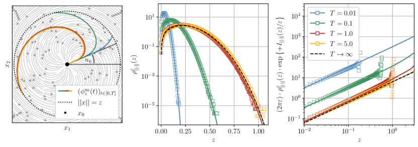
Figure 3: Left: Sketch of instanton trajectories $(\phi^{u_{0}}_{z}(t))_{t\in[0,T]}$ for different $T\in\{0.01,0.1,1,5\}$ from the example in Section 4.2 with the specific potential and swirl (221) at a fixed value of the observable $f(x)=\norm{x}=z=3$. The coloring is the same across all subfigures and explained in the right panel. All numerically obtained trajectories have been rotated to the same initial angle $u_{0}$. For small $T$, the instanton is almost radial, and for large $T$, it follows the angular component $\ell$ of the vector field $b$, with a purely radial momentum $(\theta^{u_{0}}_{z}(t))_{t\in[0,T]}$ acting against the radial force $-\nabla V$. Center and right: Comparison of the instanton and Riccati results from Section 4.2 to Monte Carlo simulations of the SDE with (221). For fixed $\varepsilon=0.05$ and the different final times $T$, we obtained $10^{8}$ samples $\norm{X^{\varepsilon}_{T}}$ each through Euler-Maruyama integration of the SDE in order to estimate the PDF $\rho^{\varepsilon}_{\norm{\cdot}}$. The resulting PDF estimate, indicated by the squares, is compared to the theoretical PDF asymptotics (177), which were obtained as detailed in Section 4.2 and are shown (without any free parameters) by the solid lines. The right subplot compares the full prefactor of the PDF, defined via $\rho^{\varepsilon}_{\norm{\cdot}}\cdot\exp\left\{+I_{\norm{\cdot}}/\varepsilon\right\}$ and obtained through direct sampling (with the same data as in the center) to the theoretical result for the quadratic approximation (solid lines).

4.3 Dynamical phase transition in a three-dimensional gradient system

For a system dimension of $n=3$, we consider a first instructive example exhibiting spontaneous symmetry breaking beyond a critical observable value $z_{\text{c}}>0$ as sketched in the right subplot of Figure 1. Choosing a gradient system

$$\differential X_{t}^{\varepsilon}=-\nabla V\left(X_{t}^{\varepsilon}\right)\differential t+\sqrt{2\varepsilon}\>\differential B_{t}\,,\quad X_{0}^{\varepsilon}=x_{0}$$ (223)

on the time interval $[0,T]$ and focusing on the stationary limit $T\to\infty$ allows us to treat this case in an exact manner. We assume that the potential has a unique global minimum at $x_{0}=(0,0,0)$ with $\nabla^{2}V(x_{0})$ positive definite. Furthermore, $V$ should be symmetric in the first component $x_{1}$, i.e. $V(-x_{1},x_{2},x_{3})=V(x_{1},x_{2},x_{3})$, and rotationally symmetric in $(x_{2},x_{3})$ for any $x_{1}$, i.e. for all $x_{1}\in\mathds{R}$ and $b\geq 0$, $V(x_{1},b\cos u,b\sin u)$ is constant in $u\in[0,2\pi)$. We assume that there exists $z_{\text{c}}>0$, such that for all $x_{1}=z\in\mathds{R}$ with $\absolutevalue{z}<z_{\text{c}}$, the function $V(z,\cdot,\cdot):\mathds{R}^{2}\to\mathds{R}$ has a unique, nondegenerate global minimum at $(x_{2},x_{3})=(0,0)$, and for all $z$ with $\absolutevalue{z}>z_{\text{c}}$, $V(z,\cdot,\cdot)$ has a continuous family of global minima at $(\bar{x}(z)\cos u,\bar{x}(z)\cos u)$ with $\bar{x}(z)>0$ and $u\in[0,2\pi)$, as sketched in Figure 4 (left). A specific example of such a potential is

$$V(x_{1},x_{2},x_{3})=V_{0}\left[\left(\frac{x_{1}}{z_{\text{c}}}\right)^{2}\frac{\left(x_{2}^{2}+x_{3}^{2}\right)^{2}}{a^{4}}+\left(1-\left(\frac{x_{1}}{z_{\text{c}}}\right)^{2}\right)\frac{x_{2}^{2}+x_{3}^{2}}{a^{2}}+\left(\frac{x_{1}}{z_{\text{c}}}\right)^{2}\right]\,,$$ (224)

with constants $V_{0},a,z_{\text{c}}>0$, which indeed exhibits a Mexican hat-like structure in the $x_{2}$-$x_{3}$ plane for $x_{1}=z>z_{\text{c}}$ with minima at radius

$$\bar{x}(z):=\frac{a}{\sqrt{2}}\sqrt{1-\left(\frac{z_{\text{c}}}{z}\right)^{2}}\,.$$ (225)

As our (linear) observable, we take

$$f=\text{pr}_{1}:\mathds{R}^{3}\to\mathds{R}\,,\quad(x_{1},x_{2},x_{3})\mapsto x_{1}\,,$$ (226)

which allows us to test the backward Riccati equation for the prefactor from Proposition 3.2 in the limit $T\to\infty$. Since the system is gradient, we known that the stationary PDF $\rho^{\varepsilon}_{\infty}:\mathds{R}^{3}\to[0,\infty)$ of $X^{\varepsilon}$ is given by

$$\rho^{\varepsilon}_{\infty}(x)=Z_{\varepsilon}^{-1}\exp\left\{-\frac{1}{\varepsilon}V(x)\right\}$$ (227)

with normalization constant

$$Z_{\varepsilon}=\int_{\mathds{R}^{3}}\exp\left\{-\frac{1}{\varepsilon}V(x)\right\}\differential^{3}x\,.$$ (228)

Applying Laplace’s method on the PDF of the marginal distribution

$$\rho^{\varepsilon}_{\text{pr}_{1}}(z)=Z_{\varepsilon}^{-1}\int_{\mathds{R}^{2}}\exp\left\{-\frac{1}{\varepsilon}V(z,x_{2},x_{3})\right\}\differential^{2}(x_{2},x_{3})$$ (229)

of the first component $X^{\varepsilon}_{1}$ (approximating both $Z_{\varepsilon}$ and the $(x_{2},x_{3})$-integral) yields

$$\rho^{\varepsilon}_{\text{pr}_{1}}(z)\overset{\varepsilon\downarrow 0}{\sim}\begin{cases}(2\pi\varepsilon)^{-1/2}\left[\frac{{\det}_{3}\nabla^{2}V(x_{0})}{{\det}_{2}\nabla^{2}V(z,0,0)}\right]^{1/2}\exp\left\{-\frac{1}{\varepsilon}\left(V(z,0,0)-V(x_{0})\right)\right\}\,,\quad&\absolutevalue{z}<z_{\text{c}}\\ (2\pi\varepsilon)^{-1}\left[\frac{{\det}_{3}\nabla^{2}V(x_{0})}{{\det}_{1}^{\prime}\nabla^{2}V(z,\bar{x}(z)\cos u_{0},\bar{x}(z)\sin u_{0})}\right]^{1/2}2\pi\bar{x}(z)\;\times\\ \quad\times\exp\left\{-\frac{1}{\varepsilon}\left(V(z,\bar{x}(z)\cos u_{0},\bar{x}(z)\sin u_{0})-V(x_{0})\right)\right\}\,,\quad&\absolutevalue{z}>z_{\text{c}}\end{cases}$$ (230)

for any $u_{0}\in D=[0,2\pi)$. Here, ${\det}_{2}$ denotes the restriction onto the $(x_{2},x_{3})$-plane, and ${\det}_{1}^{\prime}$ reduces to the single nonzero eigenvalue of the matrix in the $(x_{2},x_{3})$-plane corresponding to the radial eigenvector. For the specific example (224), the result is

$$\rho^{\varepsilon}_{\text{pr}_{1}}(z)\overset{\varepsilon\downarrow 0}{\sim}\begin{cases}(2\pi\varepsilon)^{-1/2}\frac{\sqrt{2V_{0}}}{z_{\text{c}}}\frac{1}{1-\left(z/z_{\text{c}}\right)^{2}}\exp\left\{-\frac{V_{0}}{\varepsilon}\left(\frac{z}{z_{\text{c}}}\right)^{2}\right\}\,,\quad&\absolutevalue{z}<z_{\text{c}}\\ (2\pi\varepsilon)^{-1}\frac{2\pi V_{0}}{z}\exp\left\{-\frac{V_{0}}{\varepsilon}\frac{3\left(z/z_{\text{c}}\right)^{2}-\left(z_{\text{c}}/z\right)^{2}+2}{4}\right\}\,,\quad&\absolutevalue{z}>z_{\text{c}}\end{cases}$$ (231)

as a reference result, with discontinuous second derivative of the rate function at $z=z_{\text{c}}$ and divergent prefactors as $z\uparrow z_{\text{c}}$.

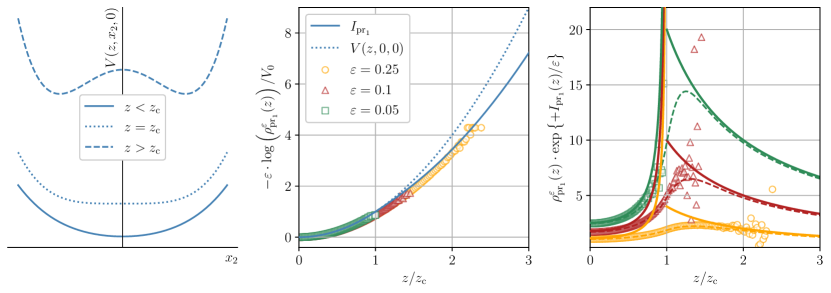
Figure 4: Left: Sketch of the potential $V$ from the example in Section 4.3 at different values of the observable $x_{1}=z$. The figure shows a cut through the $(x_{2},x_{3})$ plane at $x_{3}=0$. Note the double well/Mexican hat structure beyond $z_{\text{c}}$, which is responsible for the dynamical phase transition. Center and right: Comparison of the theoretical results from Section 4.3 to Monte Carlo simulations of the SDE (223) with the specific potential (224) (with $V_{0}=z_{\text{c}}=a=1$) as an example. For each $\varepsilon\in\left\{0.25,0.1,0.05\right\}$, about $1.3\cdot 10^{9}$ samples from the invariant measure of the SDE were obtained (with Euler-Maruyama integration steps of length $\Delta t=10^{-3}$ and sampling after each time unit) in order to estimate the PDF $\rho^{\varepsilon}_{\text{pr}_{1}}$. Center: Comparison of the Monte Carlo results on a logarithmic scale, where $-\varepsilon\cdot\log\rho^{\varepsilon}_{\text{pr}_{1}}$ collapses onto the rate function for small $\epsilon$, as expected. Note in particular that the lower branch corresponding to the symmetry-broken minima of the potential correctly matches the Monte Carlo results. Right: Comparison of the full prefactor of the PDF, defined via $\rho^{\varepsilon}_{\text{pr}_{1}}\cdot\exp\left\{+I_{\text{pr}_{1}}/\varepsilon\right\}$, obtained either through $(i)$ direct sampling (circles, triangles and squares) with the same data as in the center, or $(ii)$ numerical evaluation of the integral (229) for the marginal PDF (dashed lines), to the theoretical result for the quadratic approximation (solid lines). Note that the prefactor is correctly approximated both below and above $z_{\text{c}}$.

In order to reproduce this result using sample path large deviations, we first note that the unique (for the chosen potential) solution to the instanton equations for any endpoint $x=(x_{1},x_{2},x_{3})\in\mathds{R}^{3}$

$$\begin{cases}\dot{\phi}_{x}=-\nabla V\left(\phi_{x}\right)+2\theta_{x}\,,&\phi_{x}(0)=x_{0}\,,\quad\phi_{x}(T)=x\\ \dot{\theta}_{x}=\nabla^{2}V\left(\phi_{x}\right)^{\top}\theta_{x}\,,&\theta_{x}(T)=:\lambda_{x}\in\mathds{R}^{3}\,,\end{cases}$$ (232)

is given by

$$\dot{\phi}_{x}=\nabla V(\phi_{x})=\theta_{x}$$ (233)

as $T\to\infty$, i.e. by time-reversed deterministic dynamics, such that

$$S\left[\phi_{x}\right]=\int_{0}^{\infty}\norm{\theta_{x}}_{3}^{2}\differential t=\int_{0}^{\infty}\left\langle\nabla V(\phi_{x}),\dot{\phi}_{x}\right\rangle_{3}\differential t=V(x)-V(x_{0})\,.$$ (234)

By the contraction principle, i.e. by minimizing this result over all $(x_{2},x_{3})\in\mathds{R}^{2}$ for a given $x_{1}=z\in\mathds{R}$, we obtain the correct rate function

$$I_{\text{pr}_{1}}(z)=\left.\begin{cases}S\left[\phi_{(z,0,0)}\right]\,,\;&\absolutevalue{z}\leq z_{\text{c}}\\ S\left[\phi_{(z,\bar{x}(z)\cos u_{0},\bar{x}(z)\sin u_{0})}\right]\,,\;&\absolutevalue{z}>z_{\text{c}}\,.\end{cases}\right\}=\begin{cases}V(z,0,0)-V(x_{0})\,,v&\absolutevalue{z}\leq z_{\text{c}}\\ V(z,\bar{x}(z)\cos u_{0},\bar{x}(z)\sin u_{0})-V(x_{0})\,,\;&\absolutevalue{z}>z_{\text{c}}\,.\end{cases}$$ (235)

with any $u_{0}\in D=[0,2\pi)$. For the prefactor in the nondegenerate case $\absolutevalue{z}<z_{\text{c}}$, we first evaluate $\exp\left\{\int_{0}^{\infty}\tr\left[W_{z}\right]\right\}$ following Grafke et al. (2021): The backward Riccati matrix $W_{z}$ solves

$$\dot{W}_{z}=-2W_{z}^{2}+\nabla^{2}V(\phi_{z})W_{z}+W_{z}\nabla^{2}V(\phi_{z})+\derivative{t}\left(\nabla^{2}V(\phi_{z})\right)\,,\quad W_{z}(\infty)=0\,.$$ (236)

Defining $W_{z}=C_{z}^{-1}\dot{C}_{z}$ with $C_{z}(\infty)=1_{3\times 3}$, $\dot{C}_{z}(\infty)=0_{3\times 3}$, we have, on the one hand,

$${\det}_{3}C_{z}(0)={\det}_{3}C_{z}(\infty)\exp\left\{-\int_{0}^{\infty}\tr\left[W_{z}\right]\differential t\right\}\,,$$ (237)

and on the other hand, from (236),

$$\derivative{t}\left(\dot{C}_{z}-C_{z}\nabla^{2}V(\phi_{z})\right)=-\left(\dot{C}_{z}-C_{z}\nabla^{2}V(\phi_{z})\right)W_{z},,$$ (238)

so

$$\frac{{\det}_{3}\left(\dot{C}_{z}(\infty)-C_{z}(\infty)\nabla^{2}V(\phi_{z}(\infty))\right)}{{\det}_{3}\left(\dot{C}_{z}(0)-C_{z}(0)\nabla^{2}V(\phi_{z}(0))\right)}=\exp\left\{-\int_{0}^{\infty}\tr\left[W_{z}\right]\differential t\right\}\,.$$ (239)

Using the boundary conditions and equation (237) as well as noting that necessarily $\dot{C}_{z}(0)=0_{3\times 3}$ in the stationary limit, we obtain

$$\exp\left\{\int_{0}^{\infty}\tr\left[W_{z}\right]\differential t\right\}=\left[\frac{{\det}_{3}\left(\nabla^{2}V(x_{0})\right)}{{\det}_{3}\left(C_{z}(\infty)\nabla^{2}V(z,0,0)-\dot{C}_{z}(\infty)\right)}\right]^{1/2}=\left[\frac{{\det}_{3}\left(\nabla^{2}V(x_{0})\right)}{{\det}_{3}\left(\nabla^{2}V(z,0,0)\right)}\right]^{1/2}\,.$$ (240)

The second ingredient for the PDF prefactor is

$$\left[\left.\derivative{\lambda}\right|_{\lambda_{z}}\text{pr}_{1}(\phi_{z}(\infty))\right]^{-1/2} =\left[\left(\nabla_{\theta_{x}(\infty)}\phi_{x}(\infty)\right)_{11}\right]^{-1/2}=\left[\left(\nabla_{\phi_{x}(\infty)}\theta_{x}(\infty)\right)^{-1}_{11}\right]^{-1/2}$$

$$\overset{\eqref{eq:grad-inst-solu}}{=}\left[\left(\nabla^{2}V(z,0,0)\right)^{-1}_{11}\right]^{-1/2}=\left[\frac{{\det}_{3}\left(\nabla^{2}V(z,0,0)\right)}{{\det}_{2}\left(\nabla^{2}V(z,0,0)\right)}\right]^{1/2}\,,$$ (241)

thereby correctly reproducing the reference result below the critical observable value $z_{\text{c}}$ from (230) via Propositions 2.2 and 2.3.

Above the critical observable value $z_{\text{c}}$, the final condition for the backward Riccati equation becomes

$$W_{z}(\infty)=-\tilde{\psi}^{u_{0}}_{z}\otimes\tilde{\psi}^{u_{0}}_{z}\,,$$ (242)

where $\tilde{\psi}^{u_{0}}_{z}$ is, in particular, a unit eigenvector corresponding to the single vanishing eigenvalue of the Hessian $\nabla^{2}V(z,\bar{x}(z)\cos u_{0},\bar{x}(z)\sin u_{0})$. Setting $\dot{C}_{z}(\infty)=-\tilde{\psi}^{u_{0}}_{z}\otimes\tilde{\psi}^{u_{0}}_{z}$ in the computation above yields

$$\exp\left\{\int_{0}^{\infty}\tr\left[W_{z}^{u_{0}}\right]\differential t\right\}=\left[\frac{{\det}_{3}\left(\nabla^{2}V(x_{0})\right)}{{\det}_{3}\left(\nabla^{2}V(z,\bar{x}(z)\cos u_{0},\bar{x}(z)\sin u_{0})+\tilde{\psi}^{u_{0}}_{z}\otimes\tilde{\psi}^{u_{0}}_{z}\right)}\right]^{1/2}\,.$$ (243)

Hence, as desired, the modified initial condition renders the fraction well defined by replacing the single zero eigenvalue of the matrix in the denominator by $1$. Furthermore, we have

$$\left[\left.\derivative{\lambda}\right|_{\lambda_{z}}\text{pr}_{1}(\phi_{z}(\infty))\right]^{-1/2} =\left[\left(\nabla_{\theta_{x}(\infty)}\phi_{x}(\infty)\right)_{11}\right]^{-1/2}=\left[\left(\left.\left(\nabla_{\theta_{x}(\infty)}\phi_{x}(\infty)\right)\right|_{\left(\tilde{\psi}^{u_{0}}_{z}\right)^{\perp}}\right)_{11}\right]^{-1/2}$$

$$=\left[\left(\left.\left(\nabla^{2}V(z,\bar{x}(z)\cos u_{0},\bar{x}(z)\sin u_{0})\right)\right|_{\left(\tilde{\psi}^{u_{0}}_{z}\right)^{\perp}}\right)_{11}^{-1}\right]^{-1/2}$$

$$=\left[\frac{{\det}_{3}\left(\nabla^{2}V(z,\bar{x}(z)\cos u_{0},\bar{x}(z)\sin u_{0})+\tilde{\psi}^{u_{0}}_{z}\otimes\tilde{\psi}^{u_{0}}_{z}\right)}{{\det}_{1}^{\prime}\left(\nabla^{2}V(z,\bar{x}(z)\cos u_{0},\bar{x}(z)\sin u_{0})\right)}\right]^{1/2}\$$ (244)

by restricting to the invariant subspace $\left(\tilde{\psi}^{u_{0}}_{z}\right)^{\perp}$ of the Hessian $\nabla^{2}V(z,\bar{x}(z)\cos u_{0},\bar{x}(z)\sin u_{0})$ on which it is invertible for the computations, and afterwards reintroducing the full matrix including the modified eigenvalue $1$. All in all, we have thus correctly reproduced the PDF prefactor above the critical value in (230). For the specific example potential (224), the situation considered here is sketched and compared to the results of Monte Carlo simulations of the SDE (223) in Figure 4.

4.4 Average surface height for the one-dimensional KPZ equation with flat initial condition

The KPZ equation Kardar et al. (1986), an SPDE describing nonlinear surface growth, and in particular its large deviation statistics have been the subject of various studies. Here, particularly noteworthy works are Janas et al. (2016); Krajenbrink and Le Doussal (2017); Smith et al. (2018a); Hartmann et al. (2021) for an investigation of a short time dynamical phase transition for the distribution of the surface height at one point in space, starting from a stationary surface. Furthermore, recently, in Krajenbrink and Le Doussal (2021), an exact computation of the rate function for the same observable with general deterministic initial condition has been carried out; and for the flat initial condition, the exact distribution of the height at one point in space for all times has already been found in Calabrese and Le Doussal (2011). A systematic short-time expansion for the height distribution at one point and droplet and Brownian initial conditions, which goes beyond the rate function and includes subleading prefactor terms, can be found in Krajenbrink et al. (2018). All of the works listed above deal with the KPZ equation on an unbounded spatial domain. Here, we proceed in the spirit of Janas et al. (2016); Krajenbrink and Le Doussal (2017); Smith et al. (2018a); Hartmann et al. (2021), but modify the setup to study continuous symmetry breaking instead of only a discrete mirror symmetry. Accordingly choosing the spatially averaged surface height as an observable necessitates considering a bounded spatial domain. For such a domain, the large deviation statistics of the surface height at one point have been computed in detail in Smith et al. (2018b), with the analysis of the spatially averaged surface height left as a future task there and predicted to display a second order dynamical phase transition. Here, we will confirm this prediction and compute the leading order PDF prefactors for both phases numerically. Furthermore, we analytically compute the PDF prefactor when the spatially homogeneous instanton dominates, which, in particular, allows us to determine the critical observable value $z_{\text{c}}$. We will focus on a single choice of the only parameter of the system, the non-dimensionalized domain size $l$, and use $l=\pi$ throughout this paper. We remark that it would be an interesting future work to systematically study the large deviation properties of the system for different domain sizes $l$ using the methods developed here, and to derive a complete phase diagram in the $(l,z)$ plane for the system, similar to Smith et al. (2018b).

To be more precise, we consider the KPZ equation in one spatial dimension on a bounded interval in space $[0,L]$ with periodic boundary conditions for the surface height $H\colon[0,L]\times[0,T]\to\mathds{R}$,

$$\partial_{t}H(x,t)=\nu\partial_{xx}H(x,t)+\frac{\lambda}{2}\left(\partial_{x}H(x,t)\right)^{2}+\sqrt{D}\eta(x,t)\,,$$ (245)

starting from a flat initial profile $H(\cdot,0)=H_{0}\equiv 0$, and are interested in precise asymptotic estimates for the probability distribution (and in particular its tails) of the spatially averaged surface height at time $T$,

$$f(H(\cdot,T)):=\frac{1}{L}\int_{0}^{L}H(x,T)\;\differential x\,,$$ (246)

for small $T$. In (245), we denote by $\nu>0$ the diffusivity, by $\lambda>0$ (the choice of sign is without loss of generality) the strength of the nonlinearity, and by $D>0$ the noise strength. The noise term $\eta$ is assumed to be space-time white Gaussian noise with

$$\mathds{E}\left[\eta(x,t)\right]=0\,,\quad\mathds{E}\left[\eta(x,t)\eta(x^{\prime},t^{\prime})\right]=\delta(x-x^{\prime})\delta(t-t^{\prime})\,.$$ (247)

The non-dimensionalization $t\to tT$, $x\to\sqrt{\nu T}x$ , $H\to 2\nu H/\lambda$ and $\eta\to\left(\nu T^{3}\right)^{-1/4}\eta$ leads to the following model that we will consider for all computations in the following: For a dimensionless noise strength $\varepsilon=D\lambda^{2}T^{1/2}/(4\nu^{5/2})>0$, we consider $H^{\varepsilon}\colon[0,l]\times[0,1]\to\mathds{R}$ with $l=L/\sqrt{\nu T}$ the solution of

$$\begin{cases}\partial_{t}H^{\varepsilon}=\partial_{xx}H^{\varepsilon}+\left(\partial_{x}H^{\varepsilon}\right)^{2}+\sqrt{\varepsilon}\eta\,,\\ H^{\varepsilon}(\cdot,0)=H_{0}\equiv 0\,,\\ H^{\varepsilon}(0,t)=H^{\varepsilon}(l,t)\,,\quad\partial_{x}H^{\varepsilon}(0,t)=\partial_{x}H^{\varepsilon}(l,t)\quad\forall t\in[0,1]\,.\end{cases}$$ (248)

and are interested in estimating the PDF of the mean surface height

$$f(H^{\varepsilon}(\cdot,1)):=\frac{1}{l}\int_{0}^{l}H^{\varepsilon}(x,1)\,\differential x$$ (249)

at the final time as $\varepsilon\downarrow 0$. The small noise limit in these dimensionless variables can be seen to directly correspond to either of the limits $D\downarrow 0$ or $\lambda\downarrow 0$ in the physical variables. Additionally, as mentioned above, we choose a fixed and finite non-dimensionalized domain size $l=\pi$ in all of our numerical computations , so the usual short-time limit $T\downarrow 0$ considered in KPZ large deviations actually corresponds to simultaneously taking $T\downarrow 0$ and $\nu\propto T^{-1}\uparrow\infty$ in this setup if the physical domain size remains constant.

For spatially white noise, the KPZ equation (248) is only well-posed after renormalization, the noise being too rough for the nonlinearity $-\tfrac{1}{2}\left(\partial_{x}H^{\varepsilon}\right)^{2}$ to make sense otherwise Quastel (2011); Hairer (2013). While this is not an issue on the level of instanton computations, the solutions of which are expected to be classically differentiable, renormalization is necessary when dealing with the random fluctuations around the instanton. We interpret (248) as the result of applying a Cole-Hopf transformation to the field ${\cal Q}^{\varepsilon}\colon[0,l]\times[0,1]\to(0,\infty)$, solving the well-posed stochastic heat equation (SHE) with multiplicative noise in the Itô sense

$$\begin{cases}\partial_{t}{\cal Q}^{\varepsilon}=\partial_{xx}{\cal Q}^{\varepsilon}+\sqrt{\varepsilon}{\cal Q}^{\varepsilon}\eta\,,\\ {\cal Q}^{\varepsilon}(\cdot,0)=1\,.\end{cases}$$ (250)

Then, the height field of the KPZ equation (248) is given by

$$H^{\varepsilon}=\log{\cal Q}^{\varepsilon}\,,$$ (251)

and a formal application of Itô’s lemma shows that the Cole-Hopf transformation generates a counter-term $-\delta(0)$, where $\delta$ is Dirac’s delta function, on the right-hand side of (248) that intuitively cancels the divergences in the original KPZ equation. We will compute the contribution of the Gaussian fluctuations to the distribution of the observable (249) within this interpretation of the KPZ equation, i.e. actually consider the observable

$$F({\cal Q}^{\varepsilon}(\cdot,1)):=\frac{1}{l}\int_{0}^{l}\log{\cal Q}^{\varepsilon}(x,1)\,\differential x$$ (252)

for the SHE.

The instanton equations (5) for the example (248) and (249) that determine the instanton $(h_{z},\tilde{h}_{z},\lambda_{z})$ written in terms of the original field and its conjugate momentum read (see Fogedby (1999) for an early reference that derives these equations)

$$\begin{cases}\partial_{t}h_{z}=\partial_{xx}h_{z}+\left(\partial_{x}h_{z}\right)^{2}+\tilde{h}_{z}\,,&h_{z}(\cdot,0)\equiv 0\,,\quad f\left(h_{z}(\cdot,1)\right)=\frac{1}{l}\int_{0}^{l}h_{z}(x,1)\,\differential x=z\\ \partial_{t}\tilde{h}_{z}=-\partial_{xx}\tilde{h}_{z}+2\partial_{x}\left(\tilde{h}_{z}\partial_{x}h_{z}\right)\,,&\tilde{h}_{z}(\cdot,T)=\lambda_{z}\nabla f\left(h_{z}(\cdot,T)\right)\equiv\frac{\lambda_{z}}{l}\,.\end{cases}$$ (253)

In terms of the SHE, the instanton equations for the fields $(q_{z},p_{z},\lambda_{z})$ with

$$q_{z}=\exp\left\{h_{z}\right\}\,,\quad p_{z}=\tilde{h}_{z}\exp\left\{-h_{z}\right\}$$ (254)

become

$$\begin{cases}\partial_{t}q_{z}=\partial_{xx}q_{z}+q_{z}^{2}p_{z}\,,&q_{z}(\cdot,0)\equiv 1\,,\quad F\left(q_{z}(\cdot,1)\right)=\frac{1}{l}\int_{0}^{l}\log q_{z}(x,1)\,\differential x=z\\ \partial_{t}p_{z}=-\partial_{xx}p_{z}-q_{z}p_{z}^{2}\,,&p_{z}(\cdot,T)=\lambda_{z}\nabla F\left(q_{z}(\cdot,T)\right)\equiv\frac{\lambda_{z}}{lq_{z}(\cdot,T)}\,.\end{cases}$$ (255)

The idea is now that a trivial spatially homogeneous critical point $(h_{z}^{\text{hom}},\tilde{h}_{z}^{\text{hom}},\lambda_{z}^{\text{hom}})$ of the action functional for the average height observable, i.e. a solution of (253), is always given by

$$h_{z}^{\text{hom}}(x,t)=zt\,,\quad\tilde{h}_{z}^{\text{hom}}(x,t)=z\,,\quad\lambda_{z}^{\text{hom}}=lz\,,$$ (256)

with corresponding SHE instantons

$$q_{z}^{\text{hom}}(x,t)=\exp\left\{zt\right\}\,,\quad p_{z}^{\text{hom}}(x,t)=z\exp\left\{-zt\right\}\,,\quad\lambda_{z}^{\text{hom}}=lz\,,$$ (257)

leading to the Gaussian rate function

$$I_{f}^{\text{hom}}(z)=S\left[h_{z}^{\text{hom}}\right]=\frac{1}{2}lz^{2}$$ (258)

for all such $z\in\mathds{R}$ for which this critical point realizes the global minimum of the action under the boundary condition $f\left(h_{z}(\cdot,1)\right)=z$. However, one might expect (with reference to the typical growth patterns of the KPZ equation due to the nonlinearity and diffusion, as sketched in Kardar et al. (1986), as well as the results and scaling estimates of Smith et al. (2018b)) that for sufficiently large $z>z_{\text{c}}$ in the right tail of the distribution of $f\left(H^{\varepsilon}(\cdot,1)\right)$, the KPZ nonlinearity will favor a nonuniform surface growth in order to achieve a large average height, such that the rate function displays a non-equilibrium phase transition to a continuous family of spatially localized global minimizers $\left\{\left(h_{z}^{\text{loc},u_{0}},\tilde{h}_{z}^{\text{loc},u_{0}},\lambda_{z}^{\text{loc}}\right)\big{\mid}u_{0}\in[0,l)\right\}$ of the instanton equations. This intuitive picture is indeed confirmed by our numerical computations of instantons for this example, performed directly for (253). The corresponding results for the rate function as well as the space-time evolution of typical instantons are shown in Figure 5. For these instanton computations, we used a pseudo-spectral discretization in terms of $n_{x}=128$ Fourier modes in space $[0,l]$ with $l=\pi$ and a second-order explicit Runge-Kutta integrator in time $[0,1]$ with an integrating factor for the diffusion terms with $n_{t}=2\cdot 10^{4}$ equidistant time steps of size $\Delta t=5\cdot 10^{-5}$. The comparably high resolution in time turned out to be necessary for the subsequent Riccati equation integrations, for which the instantons serve as an input, as detailed below. In order to directly compute instantons for different and given observable values $z$, equidistantly spaced in $[-10,20]$, we use a penalty-type method, and minimized the action using L-BFGS steps with exact discrete adjoint gradient evaluations in order to reduce the $L^{2}$-norm of the action gradient by a factor of $10^{6}$ in each subproblem. For details on the optimization procedure, we refer the reader to Schorlepp et al. (2022).

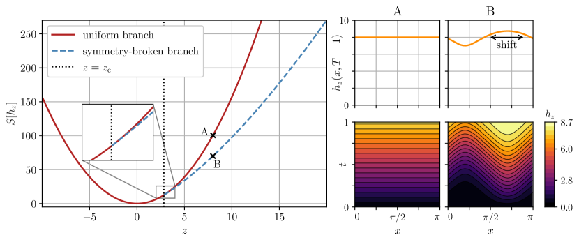
Figure 5: Results of the numerical instanton computations for the non-dimensionalized one-dimensional KPZ equation (248) and average surface height observable (249) for different heights $z$. Left: The action $S[h_{z}]$ of the two different branches that were found; on the one hand, a Gaussian branch (258) stemming from the critical point (256) which is uniform in space and shown as a solid line, and on the other hand, a branch given by localized and spatially non-uniform instantons that splits off at $z_{\text{c}}\approx 2.8259$, indicated by the dotted vertical line, as derived analytically in Appendix C. The inset shows a zoom onto the critical point, suggesting a second-order phase transition (see the left subplot of Figure 6 for the first derivative of the rate function). Two specific instanton configurations, both with $z=8$, are labeled by A and B and visualized in the right half of the figure. Center and right: Each column shows one instanton height profile $h_{z}$ as marked in the left subplot; the top row shows the height profile at the final instance in time and the bottom row shows the full space-time history of the instanton height profiles. Both columns use the same axis scaling and color map normalization.

From the results of the instanton computations, we see that this constitutes an example of a dynamical phase transition in an irreversible SPDE where the associated symmetry that is broken is continuous, thereby allowing us to apply the methods developed in the previous section in order to compute not only the large deviation rate function, given by the pointwise minimum of the two branches in Figure 5, but also a more refined, asymptotically sharp prefactor estimate. The phase transition is second order, as can be seen from the derivative of the rate function in the left subplot of Figure 6, and we also show the $L^{2}$ norm of $\partial_{x}h_{z}$ for the instantons as an order parameter for the different phases in the center subplot of Figure 6. Since the KPZ equation is a non-equilibrium system, in contrast to the previous example 4.3, the complete Riccati formalism and the corresponding numerical integration of a Riccati partial differential equation with regularized boundary data is now required to get the leading order prefactor.

When the spatially homogeneous instanton dominates, the rate function of the average surface height in the small noise limit is Gaussian with

$$\rho_{F}^{\varepsilon}(z)\overset{\varepsilon\downarrow 0}{\sim}\left(2\pi\varepsilon\right)^{-1/2}\underbrace{l^{1/2}}_{=\left[\derivative{z}\lambda_{z}^{\text{hom}}\right]^{1/2}}\,R_{z}\,\exp\{-\frac{1}{\varepsilon}\underbrace{\tfrac{1}{2}lz^{2}}_{=I_{f}^{\text{hom}}(z)}\bigg{\}}\,,$$ (259)

but the prefactor component $R_{z}$ can still depend nontrivially on $z$. The only restriction on the function $R_{\cdot}$ is that at $z=0$, we have $R_{0}=1$ for correct normalization of the PDF as $\varepsilon\downarrow 0$. In the case of the spatially homogeneous instanton, the prefactor component $R_{z}$ can be found analytically using probabilistic methods without explicit reference to the functional integration methods developed here, which is carried out in detail in Appendix C. The analysis of $R_{z}$ for the homogeneous instantons in particular yields the prediction that the critical observable value $z_{\text{c}}$ for the second order phase transition, where the $(k=1)$-contribution to the prefactor is found to diverge, is the smallest nontrivial real solution of the equation

$$\tan\left(\frac{2\pi}{l}\sqrt{2z_{\text{c}}(l)-\left(\frac{2\pi}{l}\right)^{2}}\right)+\left(\frac{2\pi}{l}\right)^{-1}\sqrt{2z_{\text{c}}(l)-\left(\frac{2\pi}{l}\right)^{2}}=0\,,$$ (260)

for $l=\pi$ and hence $z_{\text{c}}(l=\pi)\approx 2.8259$ as sketched in Figure 5, which matches the numerical results of the instanton computations quite well.

Now, we turn to the numerical prefactor computation in the SHE formulation using Riccati fields. We use the backward Riccati formalism from Proposition 3.3. The result for the PDF of $F({\cal Q}^{\varepsilon}(\cdot,1))$ as $\varepsilon\downarrow 0$ is given by

$$\rho_{F}^{\varepsilon}(z)\overset{\varepsilon\downarrow 0}{\sim}\begin{cases}\left(2\pi\varepsilon\right)^{-1/2}R_{z}\left[\derivative{z}\lambda_{z}^{\text{hom}}\right]^{1/2}\exp\left\{-\frac{1}{\varepsilon}S\left[h_{z}^{\text{hom}}\right]\right\}\,,\quad&z<z_{\text{c}}\,,\\ \left(2\pi\varepsilon\right)^{-1}\tilde{R}_{z}\left[\derivative{z}\lambda_{z}^{\text{loc}}\right]^{1/2}\exp\left\{-\frac{1}{\varepsilon}S\left[h_{z}^{\text{loc},u_{0}}\right]\right\}\,,\quad&z>z_{\text{c}}\,.\end{cases}$$ (261)

In (261), the prefactor components

$$R_{z}=\exp\left\{\frac{1}{2}\int_{0}^{1}\differential t\int_{0}^{l}\differential x\left(q_{z}^{\text{hom}}(x,t)\right)^{2}W_{z}(x,x,t)\right\}$$ (262)

and

$$\tilde{R}_{z} =lV\left(z;q_{z}^{\text{loc},u_{0}},\psi_{z}^{u_{0}}\right)\exp\left\{\frac{1}{2}\int_{0}^{1}\differential t\int_{0}^{l}\differential x\left(q_{z}^{\text{loc},u_{0}}(x,t)\right)^{2}W_{z}^{u_{0}}(x,x,t)\right\}$$ (263)

with volume factor

$$V\left(z;q_{z}^{\text{loc},u_{0}},\psi_{z}^{u_{0}}\right):=\left[\int_{0}^{l}\left(\psi_{z}^{u_{0}}(x,1)\right)^{2}\left(1-\frac{\lambda_{z}^{\text{loc}}}{l}\frac{1}{\left(q_{z}^{\text{loc},u_{0}}(x,1)\right)^{2}}\right)\differential x\right]^{1/2}$$ (264)

depend on the backward Riccati field $W_{z}\colon[0,l]^{2}\times[0,1]\to\mathds{R}$ solving

$$\partial_{t}W_{z}(x,y,t) =-\left(p_{z}(x,t)\right)^{2}\delta(x-y)-\left(\partial_{xx}+\partial_{yy}\right)W_{z}(x,y,t)$$

$$\quad-2\left(q_{z}(x,t)p_{z}(x,t)+q_{z}(y,t)p_{z}(y,t)\right)W_{z}(x,y,t)-\int_{0}^{l}W_{z}(x,x^{\prime},t)\left(q_{z}(x^{\prime},t)\right)^{2}W_{z}(x^{\prime},y,t)\differential x^{\prime}\,,$$ (265)

for both cases along the respective instantons, and with final condition

$$W_{z}(x,y,1)=-\frac{\lambda_{z}^{\text{hom}}}{l}\frac{\delta(x-y)}{\left(q_{z}^{\text{hom}}(x,1)\right)^{2}}$$ (266)

for the homogeneous instanton and

$$W_{z}^{u_{0}}(x,y,1) =-\frac{\lambda_{z}^{\text{loc}}}{l}\frac{\delta(x-y)}{\left(q_{z}^{\text{loc},u_{0}}(x,1)\right)^{2}}-\left(V\left(z;q_{z}^{\text{loc},u_{0}},\tilde{\psi}_{z}^{u_{0}}\right)\right)^{2}\tilde{\psi}_{z}^{u_{0}}(x,1)\tilde{\psi}_{z}^{u_{0}}(y,1)$$ (267)

for the spatially localized instanton. In all of these expressions, the zero mode is given by

$$\psi_{z}^{u_{0}}(x,t)=\partial_{x}q_{z}^{\text{loc},u_{0}}(x,t)$$ (268)

with $u_{0}\in[0,l)$ denoting the reference position of the localized instanton, and the normalized zero mode is defined by

$$\tilde{\psi}_{z}^{u_{0}}(x,1)=\frac{\psi_{z}^{u_{0}}(x,1)}{\left[\int_{0}^{l}\left(\psi_{z}^{u_{0}}(x^{\prime},1)\right)^{2}\differential x^{\prime}\right]^{1/2}}\,.$$ (269)

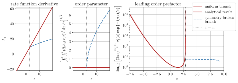
Figure 6: Left: Lagrange multiplier $\lambda_{z}$, which, by Legendre duality, is equal to the derivative of the rate function $I_{F}$, for the KPZ instantons. At the critical observable value $z=z_{\text{c}}$, the first derivative $I_{F}^{\prime}$ is continuous but not differentiable, hence the phase transition is second order. Center: The $L^{2}$ norm of the derivative $\partial_{x}h_{z}$ for the KPZ instantons as an order parameter. Right: Results of the numerical prefactor computations for the non-dimensionalized one-dimensional KPZ equation (248) and average surface height observable (249) for different heights $z$. The solid dark red line shows $R_{z}\left[\differential\lambda_{z}^{\text{hom}}/\differential z\right]^{1/2}$ as obtained from numerical solution of the backward Riccati equation (265) with numerical parameters as detailed in the main text, whereas the light red line indicates the corresponding analytical result from Appendix C, eqs. (452) and (453) (with the appearing products evaluated until $k=100$ for this figure). Beyond $z=z_{\text{c}}$, visualized by the dotted black line, the dashed blue line shows the prefactor $\tilde{R}_{z}\big{[}\differential\lambda_{z}^{\text{loc}}/\differential z\big{]}^{1/2}$, computed by solving the backward Riccati equation with modified final condition (267). Higher temporal resolution of the Riccati equation close to $t=1$ would allow to extend the results to $z>9$.

Numerically evaluating the prefactor by solving the Riccati equation and differentiating $\lambda_{z}^{\text{loc}}$ with respect to $z$ using finite differences, we obtain the results shown in the right panel of Figure 6 for the leading order prefactor

$$\lim_{\varepsilon\downarrow 0}\left[\left(2\pi\varepsilon\right)^{\frac{r(z)+1}{2}}\rho_{f}^{\varepsilon}(z)\exp\left\{+\frac{1}{\varepsilon}I_{f}(z)\right\}\right]\,,$$ (270)

where $r(z)=0$ for $z<z_{\text{c}}$ and $r(z)=1$ for $z>z_{\text{c}}$. For the solution of the Riccati equation (265), we also used a pseudo-spectral, anti-aliased code at spatial resolution $n_{x}=128$ with the Cole-Hopf transformed KPZ instantons as an input. For the time stepping, the same Heun integrator with an appropriate integrating factor in Fourier space was used, but we had to choose a different time resolution for numerical stability reasons. It turned out that the final condition (267) requires extremely small time steps in the vicinity of $t=1$, and accordingly, we divided the time interval $[0,1]$ into two subintervals $I_{1}=[0,t_{0}]$ and $I_{2}=[t_{0},1]$ with time steps of a different, smaller size $\Delta t_{2}$ within $I_{2}$ compared to $\Delta t_{1}$ within $I_{1}$. All results shown in Figure 6 were generated using $t_{0}=0.99995$, $\Delta t_{1}\approx 1.1\cdot 10^{-5}$ and $\Delta t_{2}=5\cdot 10^{-9}$ with $n_{t}=10^{5}$ time steps in total. Further increasing the resolution would allow to extend the dashed curve in Figure 6 to higher values of $z$, the relevant influence being the size of $\Delta t_{2}$ here. We made sure that the results shown are invariant under modifications of $\Delta t_{1}$, $\Delta t_{2}$ and $t_{0}$ as long as these yield finite results.

From the left subplot of Figure 6, we see that for the spatially homogeneous instanton, the numerical results from solving the backward Riccati equation (265) closely match the analytical calculations from Appendix C. Further, the prefactor beyond the critical observable value $z_{\text{c}}$ only has a weak dependence on $z$, and the behavior at $z>9$ is only due to the fact that a higher time resolution would be needed there. Furthermore, we show the instanton and the corresponding solution of the Riccati equation at different times for observable values $z=2<z_{\text{c}}$ and $z=8>z_{\text{c}}$ in Figure 7. All in all, we have demonstrated with this example that the formalism developed in this paper can indeed be employed to analyze nontrivial, spatially extended non-equilibrium systems in the presence of phase transitions.

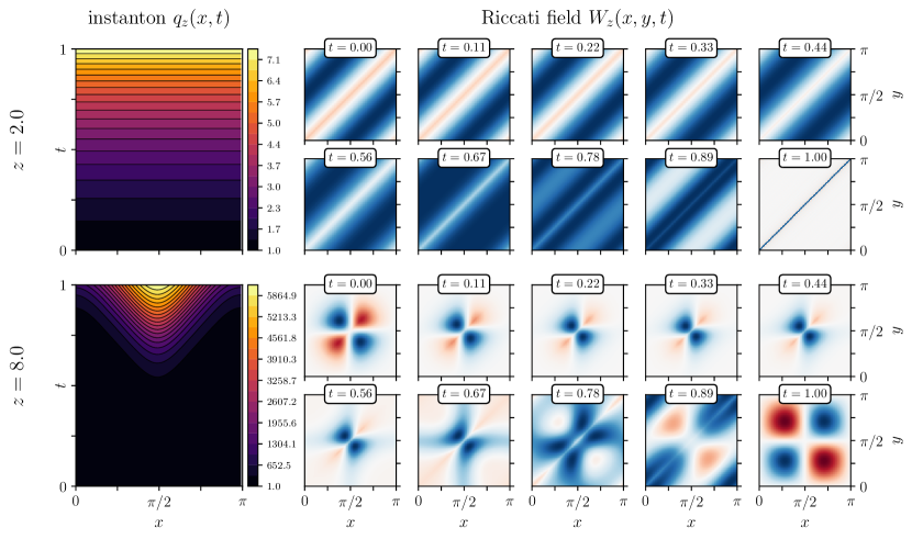
Figure 7: KPZ Instantons in SHE variables (254) (left) and corresponding backward Riccati solutions of (265) (right) for two different observable values $z=2<z_{c}$ (top row) and $z=8>z_{c}$ (bottom row). All fields were computed at $n_{x}=128$ and with $n_{t}=20000$ time steps (with uniformly spaced time steps for the instantons, and $\Delta t_{1}\approx 5.6\cdot 10^{-5}$, $\Delta t_{2}=2.5\cdot 10^{-8}$ and $t_{0}=0.99995$ for the Riccati fields). The color bar ranges for all Riccati snapshots are adjusted to the current maximum absolute value of the field and chosen to be symmetric around 0, with red symbolizing positive field values. For the spatially homogeneous case $z=2$, we see that the Riccati field remains Toeplitz for all times, starting from a Dirac $\delta$ final condition (266). For the localized case $z=8$ the final condition for $W_{z}(\cdot,\cdot,1)$ is clearly dominated by the zero mode dependent part of (267), leading to a quadrupole-like structure. For decreasing $t\downarrow 0$, the field transitions into a similar structure but with a flipped sign.

5 Discussion and Outlook

Going beyond large deviation estimates and obtaining sharp limits for rare events in stochastic systems is important for many applications, including nonequilibrium phase transitions. Importantly, one obtains the full limiting rare event probability or probability density instead of merely its exponential scaling, in regimes where direct sampling methods are completely intractable. In this paper, we have first set out to rederive such prefactor formulas at leading order for unique instantons Schorlepp et al. (2021); Grafke et al. (2021); Ferré and Grafke (2021); Bouchet and Reygner (2022), expressed in terms of Riccati matrices, explicitly using tools from field theory, i.e. by evaluating the appearing functional determinants using Forman’s theorem Forman (1987). The resulting derivations are short and conceptually simple. We stressed the role of the MGF for a vast simplification of the computations, which in particular simplifies the boundary conditions of the second variation operator in path space. Secondly, writing the prefactor in terms of operator determinants allowed us to extend the Riccati formalism to situations where the second variation around the instanton path that is used for the expansion is only positive semi-definite due to the presence of zero modes, i.e. degenerate submanifolds of instantons. We have demonstrated, using boundary-type regularizations Falco et al. (2017), that the Riccati approach remains feasible in this case, i.e. that the reduced functional determinant with removed zero eigenvalues can still be expressed through the solution of the same matrix Riccati differential equation, only with modified initial/final conditions or evaluations involving knowledge of the zero modes. Afterwards, we have verified our results in four different examples involving linear and nonlinear, reversible and irreversible SDEs as well as a nonlinear irreversible SPDE, the KPZ equation, exhibiting spontaneous symmetry breaking of the instantons for the average surface height.

With the general treatment of zero modes completed, it is now theoretically possible to compute leading order large deviation prefactors even for multi-dimensional SPDEs such as the two-dimensional or three-dimensional Navier-Stokes equations where spontaneous symmetry breaking of the rotational symmetry of instantons has indeed been observed Falkovich and Lebedev (2011); Schorlepp et al. (2022). The remaining complication for numerical computations is the high dimensionality of the involved Riccati matrices, and it would be interesting future work to consider low-rank approximations of the Riccati differential equations Breiten et al. (2021) in this regard, that could e.g. make use of the sparsity of the large-scale forcing typically used in turbulence simulations. Alternatively, an approach based on computing only the dominant eigenvalues of a Carleman-Fredholm determinant expression for the prefactor Arous (1988) could be used for numerical computations, which will be the subject of a future publication. Another interesting project would be the development of efficient importance sampling algorithms for rare events as e.g. in Ebener et al. (2019) for systems with non-unique instantons due to symmetry breaking.

Appendix A Forman’s theorem for the second variation of a general action functional

[Forman’s theorem for second order ordinary differential operators Forman (1987); Falco et al. (2017)]

Let $\Omega^{(i)}$, $i\in\{1,2\}$ be two second order differential operators

$$\Omega^{(i)}=P_{0}\derivative[2]{t}+P_{1}^{(i)}\derivative{t}+P_{2}^{(i)}$$ (271)

acting on functions $\gamma:[0,T]\to\mathds{R}^{n}$. Here, $P_{0},P_{1}^{(i)},P_{2}^{(i)}:[0,T]\to\mathds{R}^{n\times n}$ are matrix-valued functions. The highest-order coefficient $P_{0}$, which is identical for both $\Omega^{(1)}$ and $\Omega^{(2)}$, is assumed to be invertible. We impose boundary conditions

$$M^{(i)}\left(\begin{array}[]{c}\gamma(0)\\ \dot{\gamma}(0)\end{array}\right)+N^{(i)}\left(\begin{array}[]{c}\gamma(T)\\ \dot{\gamma}(T)\end{array}\right)=0$$ (276)

on the functions $\gamma$ on which $\Omega^{(i)}$ acts, where $M^{(i)},N^{(i)}\in\mathds{R}^{2n\times 2n}$. Then the quotient of the functional determinants of $\Omega^{(1)}$ and $\Omega^{(2)}$ under these boundary conditions, assuming $\Omega^{(2)}$ has no zero eigenvalues, is well defined and can be computed as

$$\frac{\operatorname{Det}_{M^{(1)},N^{(1)}}\left(\Omega^{(1)}\right)}{\operatorname{Det}_{M^{(2)},N^{(2)}}\left(\Omega^{(2)}\right)}=\frac{{\det}_{2n}\left(M^{(1)}\Upsilon^{(1)}(0)+N^{(1)}\Upsilon^{(1)}(T)\right)}{{\det}_{2n}\left(M^{(2)}\Upsilon^{(2)}(0)+N^{(2)}\Upsilon^{(2)}(T)\right)}\left[\frac{{\det}_{2n}\Upsilon^{(2)}(0){\det}_{2n}\Upsilon^{(2)}(T)}{{\det}_{2n}\Upsilon^{(1)}(0){\det}_{2n}\Upsilon^{(1)}(T)}\right]^{1/2}\,.$$ (277)

Here, $\Upsilon^{(i)}:[0,T]\to\mathds{R}^{2n\times 2n}$ is any fundamental system of solutions of the homogeneous first order equation

$$\Omega^{(i)}\gamma=0\;\Leftrightarrow\;\derivative{t}\left(\begin{array}[]{c}\gamma\\ \dot{\gamma}\end{array}\right)=\tilde{\Gamma}\left[\Omega^{(i)}\right]\left(\begin{array}[]{c}\gamma\\ \dot{\gamma}\end{array}\right)=\left(\begin{array}[]{c|c}0_{n\times n}&1_{n\times n}\\ \hline\cr-\left(P_{0}\right)^{-1}P_{2}^{(i)}&-\left(P_{0}\right)^{-1}P_{1}^{(i)}\end{array}\right)\left(\begin{array}[]{c}\gamma\\ \dot{\gamma}\end{array}\right)\,.$$ (286)

In the remainder of this appendix, we focus on operators originating from the second variation of a generic action functional

$$S[\phi]=\int_{0}^{T}L(\phi,\dot{\phi})\differential t$$ (287)

for paths $\phi:[0,T]\to\mathds{R}^{n}$ with boundary conditions that we do not specify in this section. Expanding the action to second order around a stationary path $\phi$ yields the following quadratic form:

$$\delta^{2}S[\phi][\gamma]=\frac{1}{2}\int_{0}^{T}\left\langle\left(\begin{array}[]{c}\gamma\\ \dot{\gamma}\end{array}\right),\left(\begin{array}[]{cc}\nabla^{2}_{\phi}L&\nabla_{\phi}\nabla_{\dot{\phi}}L\\ \nabla_{\dot{\phi}}\nabla_{\phi}L&\nabla_{\dot{\phi}}^{2}L\end{array}\right)\left(\begin{array}[]{c}\gamma\\ \dot{\gamma}\end{array}\right)\right\rangle_{2n}\differential t\,,$$ (294)

with the convention

$$\left(\nabla_{\phi}\nabla_{\dot{\phi}}L\right)_{ij}:=\frac{\partial^{2}L}{\partial\phi_{i}\partial\dot{\phi}_{j}}$$ (295)

and all derivatives of $L$ evaluated along $\phi$. We transform this expression into the form $\tfrac{1}{2}\int_{0}^{T}\left\langle\gamma,\Omega\gamma\right\rangle_{n}\differential t$ via partial integration:

$$\delta^{2}S[\phi][\gamma] =\frac{1}{2}\int_{0}^{T}\underbrace{\left\langle\dot{\gamma},\left(\nabla^{2}_{\dot{\phi}}L\right)\dot{\gamma}\right\rangle_{n}}_{=:I_{1}}+\underbrace{\left\langle\gamma,\left(\nabla_{\phi}\nabla_{\dot{\phi}}L\right)\dot{\gamma}\right\rangle_{n}+\left\langle\dot{\gamma},\left(\nabla_{\dot{\phi}}\nabla_{\phi}L\right)\gamma\right\rangle_{n}}_{=:I_{2}}+\left\langle\gamma,\left(\nabla^{2}_{\phi}L\right)\gamma\right\rangle_{n}\differential t$$

$$I_{1} =\frac{1}{2}\left.\left\langle\gamma,\left(\nabla^{2}_{\dot{\phi}}L\right)\dot{\gamma}\right\rangle_{n}\right|^{T}_{0}-\frac{1}{2}\int_{0}^{T}\left\langle\gamma,\frac{\differential}{\differential t}\left(\left(\nabla^{2}_{\dot{\phi}}L\right)\frac{\differential}{\differential t}\right)\gamma\right\rangle_{n}\differential t$$

$$I_{2} =\frac{1}{2}\int_{0}^{T}\frac{\differential}{\differential t}\left(\left\langle\gamma,\left(\nabla_{\dot{\phi}}\nabla_{\phi}L\right)\gamma\right\rangle_{n}\right)-\left\langle\gamma,\frac{\differential}{\differential t}\left(\nabla_{\dot{\phi}}\nabla_{\phi}L\right)\gamma\right\rangle_{n}+\left\langle\gamma,\left(\left[\nabla_{\phi},\nabla_{\dot{\phi}}\right]L\right)\dot{\gamma}\right\rangle_{n}\differential t$$

$$=\frac{1}{2}\left.\left\langle\gamma,\left(\nabla_{\dot{\phi}}\nabla_{\phi}L\right)\gamma\right\rangle_{n}\right|^{T}_{0}+\int_{0}^{T}\left\langle\gamma,\left(\left[\nabla_{\phi},\nabla_{\dot{\phi}}\right]L\right)\frac{\differential}{\differential t}\gamma\right\rangle_{n}-\left\langle\gamma,\frac{\differential}{\differential t}\left(\nabla_{\dot{\phi}}\nabla_{\phi}L\right)\gamma\right\rangle_{n}\differential t\,.$$ (296)

Here, $\left[\cdot,\cdot\right]$ denotes the commutator of two operators. With the definition $\theta:=\nabla_{\dot{\phi}}L$ for the conjugate momentum and hence

$$\zeta:=\left(\nabla^{2}_{\dot{\phi}}L\right)\dot{\gamma}+\left(\nabla_{\dot{\phi}}\nabla_{\phi}L\right)\gamma$$ (297)

for the momentum fluctuations, the additional boundary term that we obtain and that needs to vanish through the imposition of suitable boundary conditions (cf. main text) for the fluctuations is $\tfrac{1}{2}\left.\left\langle\gamma,\zeta\right\rangle_{n}\right|^{T}_{0}$, leaving us with

$$\delta^{2}S[\phi][\gamma]=\frac{1}{2}\int_{0}^{T}\left\langle\gamma,\left[-\frac{\differential}{\differential t}\left(\left(\nabla^{2}_{\dot{\phi}}L\right)\frac{\differential}{\differential t}\right)+\left(\left[\nabla_{\phi},\nabla_{\dot{\phi}}\right]L\right)\frac{\differential}{\differential t}+\left(\nabla_{\phi}^{2}L\right)-\frac{\differential}{\differential t}\left(\nabla_{\dot{\phi}}\nabla_{\phi}L\right)\right]\gamma\right\rangle_{n}\differential t\,.$$ (298)

Written in this way, the Jacobi operator Evans (2021), i.e. the second order linear differential operator

$$\Omega=\Omega[\phi]=\left[-\frac{\differential}{\differential t}\left(\left(\nabla^{2}_{\dot{\phi}}L\right)\frac{\differential}{\differential t}\right)+\left(\left[\nabla_{\phi},\nabla_{\dot{\phi}}\right]L\right)\frac{\differential}{\differential t}+\left(\nabla_{\phi}^{2}L\right)-\frac{\differential}{\differential t}\left(\nabla_{\dot{\phi}}\nabla_{\phi}L\right)\right]$$ (299)

realizing the second variation is $L^{2}([0,T],\mathds{R}^{n})$-self-adjoint, i.e. $\left\langle\gamma_{1},\Omega\gamma_{2}\right\rangle=\left\langle\Omega\gamma_{1},\gamma_{2}\right\rangle$ for all fluctuation paths with boundary conditions such that $\left.\left\langle\zeta_{1},\gamma_{2}\right\rangle_{n}\right|^{T}_{0}-\left.\left\langle\gamma_{1},\zeta_{2}\right\rangle_{n}\right|^{T}_{0}=0$.

For the first order equation in Forman’s theorem, we read off

$$P_{0} =-\nabla^{2}_{\dot{\phi}}L$$ (300)

$$P_{1} =\left[\nabla_{\phi},\nabla_{\dot{\phi}}\right]L-\frac{\differential}{\differential t}\left(\nabla^{2}_{\dot{\phi}}L\right)$$ (301)

$$P_{2} =\nabla^{2}_{\phi}L-\frac{\differential}{\differential t}\left(\nabla_{\dot{\phi}}\nabla_{\phi}L\right)\,.$$ (302)

The first order version of the Jacobi equation

$$\Omega[\phi]\gamma=0$$ (303)

appearing in Forman’s theorem hence becomes

$$\frac{\differential}{\differential t}\left(\begin{array}[]{c}\gamma\\ \dot{\gamma}\end{array}\right) =\tilde{\Gamma}[\Omega]\left(\begin{array}[]{c}\gamma\\ \dot{\gamma}\end{array}\right)=\left(\begin{array}[]{c|c}0_{n\times n}&1_{n\times n}\\ \hline\cr-\left(P_{0}\right)^{-1}P_{2}&-\left(P_{0}\right)^{-1}P_{1}\end{array}\right)\left(\begin{array}[]{c}\gamma\\ \dot{\gamma}\end{array}\right)$$ (312)

$$=\left(\begin{array}[]{c|c}0_{n\times n}&1_{n\times n}\\ \hline\cr\left(\nabla_{\dot{\phi}}^{2}L\right)^{-1}\left(\nabla^{2}_{\phi}L-\frac{\differential}{\differential t}\left(\nabla_{\dot{\phi}}\nabla_{\phi}L\right)\right)&\left(\nabla_{\dot{\phi}}^{2}L\right)^{-1}\left(\left[\nabla_{\phi},\nabla_{\dot{\phi}}\right]L-\frac{\differential}{\differential t}\left(\nabla^{2}_{\dot{\phi}}L\right)\right)\end{array}\right)\left(\begin{array}[]{c}\gamma\\ \dot{\gamma}\end{array}\right)\,.$$ (317)

In many application, such as in this paper, it is more natural to switch to a Hamiltonian instead of a Lagrangian formulation of the Jacobi equation. In fact, we have already seen above that the natural boundary conditions for the fluctuations include the conjugate momentum fluctuations. Due to this reason, we associate to the fundamental system of solutions $\Upsilon$ of $\Omega$, understood as a first order differential equation (317) in $(\gamma,\dot{\gamma})$, the following fundamental system of solutions

$$\tilde{\Upsilon}:=\Lambda\Upsilon\,,\quad\Lambda=\left(\begin{array}[]{c|c}1_{n\times n}&0_{n\times n}\\ \hline\cr\nabla_{\dot{\phi}}\nabla_{\phi}L&\nabla^{2}_{\dot{\phi}}L\end{array}\right)\,.$$ (320)

The transformation is invertible iff $P_{0}=-\nabla^{2}_{\dot{\phi}}L$ is invertible (which is exactly an assumption of Forman’s theorem) with

$$\Lambda^{-1}=\left(\begin{array}[]{c|c}1_{n\times n}&0_{n\times n}\\ \hline\cr-\left(\nabla^{2}_{\dot{\phi}}L\right)^{-1}\nabla_{\dot{\phi}}\nabla_{\phi}L&\left(\nabla^{2}_{\dot{\phi}}L\right)^{-1}\end{array}\right)\,.$$ (323)

A straightforward calculation then shows that

$$\frac{\differential}{\differential t}\tilde{\Upsilon}=\left(\dot{\Lambda}\Lambda^{-1}+\Lambda\dot{\Upsilon}\Lambda^{-1}\right)\tilde{\Upsilon}=:\Gamma[\Omega]\tilde{\Upsilon}$$ (324)

with

$$\Gamma[\Omega] =\left(\begin{array}[]{c|c}-\left(\nabla^{2}_{\dot{\phi}}L\right)^{-1}\left(\nabla_{\dot{\phi}}\nabla_{\phi}L\right)&\left(\nabla^{2}_{\dot{\phi}}L\right)^{-1}\\ \hline\cr\nabla^{2}_{\phi}L-\left(\nabla_{\phi}\nabla_{\dot{\phi}}L\right)\left(\nabla_{\dot{\phi}}^{2}L\right)^{-1}\left(\nabla_{\dot{\phi}}\nabla_{\phi}L\right)&\left(\nabla_{\phi}\nabla_{\dot{\phi}}L\right)\left(\nabla^{2}_{\dot{\phi}}L\right)^{-1}\end{array}\right)=\left(\begin{array}[]{c|c}\nabla_{\theta}\nabla_{\phi}H&\nabla_{\theta}^{2}H\\ \hline\cr-\nabla_{\phi}^{2}H&-\nabla_{\phi}\nabla_{\theta}H\end{array}\right)$$ (329)

$$=\left(\begin{array}[]{c|c}0_{n\times n}&1_{n\times n}\\ \hline\cr-1_{n\times n}&0_{n\times n}\end{array}\right)\left(\begin{array}[]{c|c}\nabla_{\phi}^{2}H&\nabla_{\phi}\nabla_{\theta}H\\ \hline\cr\nabla_{\theta}\nabla_{\phi}H&\nabla_{\theta}^{2}H\end{array}\right)=:J\;\nabla^{2}H\,,$$ (334)

where $J$ is the standard $2n\times 2n$ symplectic matrix. The second equality in (334) holds if $\phi$ is a critical point of the action functional, or, equivalently, $(\phi,\theta)$ is a solution of the canonical equations of motion

$$\derivative{t}\left(\begin{array}[]{c}\phi\\ \theta\end{array}\right)=J\;\nabla H(\phi,\theta)=\left(\begin{array}[]{c}\nabla_{\theta}H(\phi,\theta)\\ -\nabla_{\phi}H(\phi,\theta)\end{array}\right)$$ (339)

The Hamiltonian $H$ is defined via

$$H(\phi,\theta)=\sup_{y}\left(\left\langle\theta,y\right\rangle_{n}-L(\phi,y)\right)=\left\langle\theta,\dot{\phi}(\phi,\theta)\right\rangle-L(\phi,\dot{\phi}(\phi,\theta))\,,$$ (340)

where the second equality follows by assuming strict convexity of $L$ in $\dot{\phi}$ and solving the implicit equation $\theta=\partial L(\phi,\dot{\phi})/\partial\dot{\phi}$ for $\dot{\phi}$. Let us summarize the results of the transformation in the following proposition.

[Forman’s theorem for second variations in Hamiltonian formulation (cf. (Corazza and Fadel, 2020))] Let

$$S[\phi]=\int_{0}^{T}L(\phi,\dot{\phi})\differential t$$ (341)

be an action functional with $\nabla^{2}_{\dot{\phi}}L$ independent of $\phi$ and $\dot{\phi}$, and consider two paths $\phi_{1},\phi_{2}:[0,T]\to\mathds{R}^{n}$ that are critical points of the action. Then the quotient of functional determinants of $\Omega[\phi_{i}]$, realizing the second variation of $S$ along $\phi_{i}$ as

$$\delta^{2}S[\phi_{i}][\gamma]=\frac{1}{2}\int_{0}^{T}\left\langle\gamma(t),(\Omega[\phi_{i}]\gamma)(t)\right\rangle_{n}\differential t$$ (342)

with boundary conditions ${\cal A}_{i}$ imposed on the fluctuations, can be computed as

$$\frac{\operatorname{Det}_{M_{1},N_{1}}\left(\Omega[\phi_{1}]\right)}{\operatorname{Det}_{M_{2},N_{2}}\left(\Omega[\phi_{2}]\right)}=\frac{{\det}_{2n}\left(M_{1}\Upsilon_{1}(0)+N_{1}\Upsilon_{1}(T)\right)}{{\det}_{2n}\left(M_{2}\Upsilon_{2}(0)+N_{2}\Upsilon_{2}(T)\right)}\left[\frac{{\det}_{2n}\Upsilon_{2}(0){\det}_{2n}\Upsilon_{2}(T)}{{\det}_{2n}\Upsilon_{1}(0){\det}_{2n}\Upsilon_{1}(T)}\right]^{1/2}\,.$$ (343)

Here, $M_{i},N_{i}\in\mathds{R}^{2n\times 2n}$ impose the boundary conditions ${\cal A}_{i}$ for $(\gamma,\zeta):=(\gamma,\left(\nabla^{2}_{\dot{\phi}}L\right)\dot{\gamma}+\left(\nabla_{\dot{\phi}}\nabla_{\phi}L\right)\gamma)$ as

$$M_{i}\left(\begin{array}[]{c}\gamma(0)\\ \zeta(0)\end{array}\right)+N_{i}\left(\begin{array}[]{c}\gamma(T)\\ \zeta(T)\end{array}\right)=0\,,$$ (348)

which we assume to guarantee the condition

$$\left.\left\langle\zeta_{1},\gamma_{2}\right\rangle_{n}\right|^{T}_{0}-\left.\left\langle\gamma_{1},\zeta_{2}\right\rangle_{n}\right|^{T}_{0}=0$$ (349)

for all variations $(\gamma_{1},\zeta_{1})$ and $(\gamma_{2},\zeta_{2})$. Further, $\Upsilon_{i}:[0,T]\to\mathds{R}^{2n\times 2n}$ is any fundamental system of solutions of the Jacobi equation

$$\derivative{t}\left(\begin{array}[]{c}\gamma\\ \zeta\end{array}\right)=J\cdot\nabla^{2}H(\phi_{i},\theta_{i})\cdot\left(\begin{array}[]{c}\gamma\\ \zeta\end{array}\right)\,.$$ (354)

Remark A.0.

If the second order coefficient matrix $\nabla^{2}_{\dot{\phi}}L$ does depend on the path around which the expansion is performed, as is the case for multiplicative noise in the main text, then considering variations $\left(\nabla^{2}_{\dot{\phi}}L\right)^{-1/2}\gamma$ instead of $\gamma$ naturally leads to the computation of the ratio

$$\frac{\operatorname{Det}_{M_{1},N_{1}}\left(\left(\nabla^{2}_{\dot{\phi}}L(\phi_{1},\dot{\phi}_{1})\right)^{-1}\Omega[\phi_{1}]\right)}{\operatorname{Det}_{M_{2},N_{2}}\left(\left(\nabla^{2}_{\dot{\phi}}L(\phi_{2},\dot{\phi}_{2})\right)^{-1}\Omega[\phi_{2}]\right)}$$ (355)

instead, to which the proposition can then be applied without any further changes (note that for these new operators, the second order coefficient matrix will be negative unity, and the other coefficients are multiplied by $\left(\nabla^{2}_{\dot{\phi}}L(\phi_{i},\dot{\phi}_{i})\right)^{-1}$, which yields the same equation in (286) as before, thereby leaving (354) invariant).

Example A.0.

For the Freidlin-Wentzell Lagrangian

$$L(\phi,\dot{\phi})=\frac{1}{2}\left\langle\dot{\phi}-b(\phi),a^{-1}(\phi)\left(\dot{\phi}-b(\phi)\right)\right\rangle_{n}\,,$$ (356)

the corresponding Hamiltonian is given by

$$H(\phi,\theta)=\left\langle b(\phi),\theta\right\rangle_{n}+\frac{1}{2}\left\langle\theta,a(\phi)\theta\right\rangle_{n}\,.$$ (357)

The derivatives of $L$ and $H$ are

$$\nabla_{\dot{\phi}}L=a^{-1}(\phi)\left(\dot{\phi}-b(\phi)\right)=\theta\,,\quad\nabla_{\phi}L=-\nabla b(\phi)^{\top}\theta-\tfrac{1}{2}\left\langle\theta,\nabla a(\phi)\theta\right\rangle_{n}\,,\quad\nabla^{2}_{\dot{\phi}}L=a^{-1}(\phi)$$

$$\nabla^{2}_{\phi}L=\nabla b(\phi)^{\top}a^{-1}(\phi)\nabla b(\phi)-\left\langle\nabla^{2}b(\phi),\theta\right\rangle_{n}+\nabla b(\phi)^{\top}a^{-1}(\phi)\left(\nabla a(\phi)\theta\right)^{\top}+\dots$$

$$\dots+\left(\nabla a(\phi)\theta\right)a^{-1}(\phi)\nabla b(\phi)+\left\langle\theta,\nabla a(\phi)a^{-1}(\theta)\nabla a(\phi)\theta\right\rangle_{n}-\tfrac{1}{2}\left\langle\theta,\nabla^{2}a(\phi)\theta\right\rangle_{n}$$

$$\nabla_{\phi}\nabla_{\dot{\phi}}L=-\nabla b(\phi)^{\top}a^{-1}(\phi)-\left(\nabla a(\phi)\theta\right)^{\top}a^{-1}(\phi)\,,\quad\nabla_{\dot{\phi}}\nabla_{\phi}L=-a^{-1}(\phi)\nabla b(\phi)-a^{-1}(\phi)\left(\nabla a(\phi)\theta\right)\,,$$ (358)

and

$$\nabla_{\theta}H=b(\phi)+a\theta\,,\quad\nabla_{\phi}H=\nabla b(\phi)^{\top}\theta+\tfrac{1}{2}\left\langle\theta,\nabla a(\phi)\theta\right\rangle_{n}\,,$$

$$\quad\nabla^{2}_{\theta}H=a(\phi)\,,\quad\nabla^{2}_{\phi}H=\left\langle\nabla^{2}b(\phi),\theta\right\rangle_{n}+\tfrac{1}{2}\left\langle\theta,\nabla^{2}a(\phi)\theta\right\rangle_{n}\,,$$

$$\nabla_{\phi}\nabla_{\theta}H=\nabla b(\phi)^{\top}+\left(\nabla a(\phi)\theta\right)^{\top}\,,\quad\nabla_{\theta}\nabla_{\phi}H=\nabla b(\phi)+\left(\nabla a(\phi)\theta\right)\,,$$ (359)

where we use the notation

$$\left[\nabla a(\phi)\theta\right]_{ij}=\partial_{j}a_{ik}(\phi)\theta_{k}\,.$$ (360)

Hence

$$\Omega[\phi] =\left(-\derivative{t}-\nabla b(\phi)^{\top}-\left(\nabla a(\phi)\theta\right)^{\top}\right)a^{-1}(\phi)\left(\derivative{t}-\nabla b(\phi)-\left(\nabla a(\phi)\theta\right)\right)$$

$$\quad-\left\langle\nabla^{2}b(\phi),\theta\right\rangle_{n}-\frac{1}{2}\left\langle\theta,\nabla^{2}a(\phi)\theta\right\rangle_{n}$$ (361)

and

$$\Gamma[\phi]=\left(\begin{array}[]{c|c}\nabla b(\phi)+\left(\nabla a(\phi)\theta\right)&a(\phi)\\ \hline\cr-\left\langle\nabla^{2}b(\phi),\theta\right\rangle_{n}-\frac{1}{2}\left\langle\theta,\nabla^{2}a(\phi)\theta\right\rangle_{n}&-\nabla b(\phi)^{\top}-\left(\nabla a(\phi)\theta\right)^{\top}\end{array}\right)\,.$$ (364)

Example A.0.

For the Lagrangian

$$L(\phi,\dot{\phi})=\frac{1}{2}\norm{\dot{\phi}}_{n}^{2}+V(\phi)$$ (365)

appearing in quantum mechanics in imaginary time, with Hamiltonian

$$H(\phi,\theta)=\frac{1}{2}\norm{\dot{\phi}}_{n}^{2}-V(\phi)\,,$$ (366)

Jacobi’s equation becomes

$$\derivative{t}\left(\begin{array}[]{c}\gamma\\ \zeta\end{array}\right)=\left(\begin{array}[]{c|c}0_{n\times n}&1_{n\times n}\\ \hline\cr\nabla^{2}V(\phi)&0_{n\times n}\end{array}\right)\left(\begin{array}[]{c}\gamma\\ \zeta\end{array}\right)$$ (373)

or

$$\left[-\derivative[2]{t}+\nabla^{2}V(\phi)\right]\gamma=0\,,$$ (374)

which is the classical Gel’fand-Yaglom formula Gel’fand and Yaglom (1960); Coleman (1979).

It is well known from the calculus of variations that, if the Jacobi equation (303) has no conjugate points Levi (2014) in $[0,T]$ (“Jacobi condition”), then it is possible to construct a solution of a certain symmetric matrix Riccati differential equation Reid (1972), either forward or backward in time, out of solutions $(\gamma,\zeta):[0,T]\to\mathds{R}^{2n\times n}$ (if, depending on the solution, either $\gamma(t_{0})$ or $\zeta(t_{0})$ is invertible for any $t_{0}\in[0,T]$ and hence for all $t\in[0,T]$ Clarke and Zeidan (1986)):

• $W:=\zeta\gamma^{-1}:[0,T]\to\mathds{R}^{n\times n}$ satisfies the backward Riccati equation

  $$\dot{W}=-\nabla^{2}_{\phi}H-W\nabla_{\theta}\nabla_{\phi}H-\left(\nabla_{\phi}\nabla_{\theta}H\right)W-W\left(\nabla^{2}_{\theta}H\right)W\,.$$ (375)

• $Q=W^{-1}=\gamma\zeta^{-1}:[0,T]\to\mathds{R}^{n\times n}$ solves the forward Riccati equation

  $$\dot{Q}=\nabla^{2}_{\theta}H+Q\nabla_{\phi}\nabla_{\theta}H+\left(\nabla_{\theta}\nabla_{\phi}H\right)Q+Q\left(\nabla^{2}_{\phi}H\right)Q\,.$$ (376)

Remark A.0.

If it exists, the solution of the backward matrix Riccati equation $W$ can naturally be connected to the positive definiteness of $\delta^{2}S$ Evans (2021), which is why the fact that Riccati matrix differential equations appear in the functional determinant computations is not very surprising from a calculus of variations perspective: Observing that

$$\nabla^{2}_{\phi}L=\dot{W}+\left(W-\nabla_{\phi}\nabla_{\dot{\phi}}L\right)\left(\nabla^{2}_{\dot{\phi}}L\right)^{-1}\left(W-\nabla_{\dot{\phi}}\nabla_{\phi}L\right)$$ (377)

and inserting this expression for $\nabla^{2}_{\phi}L$ into the second variation, we obtain, assuming that $\nabla^{2}_{\dot{\phi}}L$ is positive definite (“Legendre condition”),

$$\delta^{2}S[\phi][\gamma]=\frac{1}{2}\left.\left\langle\gamma,W\gamma\right\rangle_{n}\right\rvert_{0}^{T}+\frac{1}{2}\int_{0}^{T}\norm{\left(\nabla^{2}_{\dot{\phi}}L\right)^{1/2}\left[\dot{\gamma}-\left(\nabla^{2}_{\dot{\phi}}L\right)^{-1}\left(W-\nabla_{\dot{\phi}}\nabla_{\phi}L\right)\gamma\right]}^{2}_{n}\differential t\,,$$ (378)

which can be used to show that $\delta^{2}S[\phi][\gamma]>0$ for all $\gamma\neq 0$ under appropriate boundary conditions.

Appendix B Sharp moment-generating function estimate for nondegenerate instantons from WKB analysis for a general Hamiltonian

As a reference, we state a general sharp estimate for the MGF of a final-time observable $f:\mathds{R}^{n}\to\mathds{R}$

$$A_{f}^{\varepsilon}(\lambda)=\mathds{E}_{x}\left[\exp\left\{\frac{\lambda}{\varepsilon}f\left(X_{T}^{\varepsilon}\right)\right\}\right]$$ (379)

for a $(\varepsilon>0)$-indexed family of continuous-time Markov processes $\left(X_{t}^{\varepsilon}\right)_{t\in[0,T]}$ with state space $\mathds{R}^{n}$, deterministic initial value $X^{0}=x\in\mathds{R}^{n}$ and generator $L_{\varepsilon}$ which we assume to satisfy a large deviation principle as $\varepsilon\downarrow 0$. Defining (see e.g. Feng and Kurtz (2006))

$$H_{\varepsilon}\varphi:=\varepsilon\exp\left\{-\frac{\varphi}{\varepsilon}\right\}L_{\varepsilon}\exp\left\{\frac{\varphi}{\varepsilon}\right\}$$ (380)

for test functions $\varphi\colon\mathds{R}^{n}\to\mathds{R}$ as well as the LDT Hamiltonian $H\colon\mathds{R}^{n}\times\mathds{R}^{n}\to\mathds{R}$, $(\phi,\theta)\mapsto H(\phi,\theta)$ via

$$H(\cdot,\nabla\varphi)=\lim_{\varepsilon\downarrow 0}H_{\varepsilon}\varphi,$$ (381)

we have the following result, obtained via WKB analysis of the Kolmogorov backward equation for $A_{f}^{\varepsilon}(\lambda)$:

[Sharp MGF estimate for nondegenerate instantons from WKB analysis for a general Hamiltonian] The MGF $A_{f}^{\varepsilon}$ for $\varepsilon\downarrow 0$ satisfies

$$A_{f}^{\varepsilon}(\lambda)\overset{\varepsilon\downarrow 0}{\sim}R_{\lambda}\exp\left\{\frac{1}{\varepsilon}\left(\lambda f\left(\phi_{\lambda}(T)\right)-\int\left\langle\theta_{\lambda},\differential\phi_{\lambda}\right\rangle_{n}+H(\phi_{\lambda},\theta_{\lambda})T\right)\right\}$$ (382)

with leading-order prefactor

$$R_{\lambda}=\exp\left\{\int_{0}^{T}\left(\left.\derivative{\varepsilon}\right|_{\varepsilon=0}H_{\varepsilon}S\right)_{(t,\phi_{\lambda}(t))}\differential t\right\}.$$ (383)

Here, $(\phi_{\lambda},\theta_{\lambda})$ solve the instanton equations

$$\derivative{t}\left(\begin{array}[]{c}\phi_{\lambda}\\ \theta_{\lambda}\end{array}\right)=J\nabla H(\phi_{\lambda},\theta_{\lambda})=\left(\begin{array}[]{c}\nabla_{\theta}H(\phi_{\lambda},\theta_{\lambda})\\ -\nabla_{\phi}H(\phi_{\lambda},\theta_{\lambda})\end{array}\right)\,,\quad\phi_{\lambda}(0)=x\,,\quad\theta_{\lambda}(T)=\lambda\nabla f(\phi_{\lambda}(T))\,,$$ (388)

which are the relevant characteristic for $S\colon[0,T]\times\mathds{R}^{n}\to\mathds{R}$, solving the Hamilton-Jacobi equation

$$\partial_{t}S(t,x)+H(x,\nabla S(t,x))=0\,,\quad S(T,x)=\lambda f(x)\,,$$ (389)

such that

$$\nabla S\left(t,\phi_{\lambda}(t)\right)=\theta_{\lambda}(t)\,.$$ (390)

For the evaluation of the prefactor $R_{\lambda}$, the second derivative of $S$ along the characteristic

$$\nabla^{2}S\left(t,\phi_{\lambda}(t)\right)=:W_{\lambda}(t)$$ (391)

with $W_{\lambda}\colon[0,T]\to\mathds{R}^{n\times n}$ can be found by solving the backward Riccati equation

$$\begin{cases}\dot{W}_{\lambda}=-\nabla^{2}_{\phi}H-W_{\lambda}\nabla_{\theta}\nabla_{\phi}H-\left(\nabla_{\phi}\nabla_{\theta}H\right)W_{\lambda}-W_{\lambda}\left(\nabla^{2}_{\theta}H\right)W_{\lambda}\,,\\ W_{\lambda}(T)=\lambda\nabla^{2}f(\phi_{\lambda}(T))\,.\end{cases}$$ (392)

Remark B.0.

As remarked in Grafke et al. (2021), it is possible to transfer the backward to the forward Riccati equation in general solely on the level of Riccati equations (if both are well-posed for the problem at hand), the general link being

$$\frac{{\det}_{n}\left(1_{n\times n}-W(T)Q(T)\right)}{{\det}_{n}\left(1_{n\times n}-W(0)Q(0)\right)}=\exp\left\{\int_{0}^{T}\tr\left[\left(\nabla^{2}_{\phi}H\right)Q-\left(\nabla^{2}_{\theta}H\right)W\right]\differential t\right\}$$ (393)

with $Q$ solving

$$\dot{Q}=\nabla^{2}_{\theta}H+Q\nabla_{\phi}\nabla_{\theta}H+\left(\nabla_{\theta}\nabla_{\phi}H\right)Q+Q\left(\nabla^{2}_{\phi}H\right)Q\,.$$ (394)

Derivation of Proposition B :

Analogously to Grafke et al. (2021), we define

$$u_{\varepsilon}(T-t,x)=\mathds{E}_{x}\left[\exp\left\{\frac{\lambda}{\varepsilon}f(X_{t}^{\varepsilon})\right\}\right]\,,\quad u_{\varepsilon}(T,x)=\exp\left\{\frac{\lambda}{\varepsilon}f(x)\right\}$$ (395)

such that $A_{f}^{\varepsilon}(\lambda)=u_{\varepsilon}(0,x)$ and $u_{\varepsilon}$ solves

$$\partial_{t}u_{\varepsilon}+L_{\varepsilon}u_{\varepsilon}=0\,.$$ (396)

The WKB ansatz

$$u_{\varepsilon}(t,x)=Z_{\varepsilon}(t,x)\exp\left\{\frac{S(t,x)}{\varepsilon}\right\}\,,\quad S(T,x)=\lambda f(x)\,,\quad Z_{\varepsilon}(T,x)=1\,,$$ (397)

where we later assume that $Z_{\varepsilon}=Z+{\cal O}(\varepsilon)$, leads to

$$\exp\left\{\frac{S}{\varepsilon}\right\}\left[\frac{1}{\varepsilon}Z_{\varepsilon}\partial_{t}S+\partial_{t}Z_{\varepsilon}+\frac{Z_{\varepsilon}}{\varepsilon}H_{\varepsilon}\left(S+\varepsilon\log Z_{\varepsilon}\right)\right]=0\,.$$ (398)

Expanding $H_{\varepsilon}$ yields

$$H_{\varepsilon}\left(S+\varepsilon\log Z_{\varepsilon}\right)=H(\cdot,\nabla S)+\varepsilon\left[\left.\derivative{\varepsilon}\right|_{\varepsilon=0}H_{\varepsilon}S+\left\langle\nabla_{\theta}H(\cdot,\nabla S),\frac{\nabla Z}{Z}\right\rangle_{n}\right]+{\cal O}\left(\varepsilon^{2}\right)\,,$$ (399)

so, at order $\varepsilon^{-1}$, we obtain the Hamilton-Jacobi equation

$$\partial_{t}S+H(\cdot,\nabla S)=0$$ (400)

for $S$ as expected, which can be solved by the method of characteristics, yielding the instanton equations (388). Differentiating (400) twice and plugging in the characteristics results in the Riccati equation (392). For the determination of the leading order prefactor $Z$, we note that at order $\varepsilon^{0}$,

$$\partial_{t}Z+\left\langle\nabla_{\theta}H(\cdot,\nabla S),\nabla Z\right\rangle_{n}+\left(\left.\derivative{\varepsilon}\right|_{\varepsilon=0}H_{\varepsilon}S\right)Z=0\,.$$ (401)

so evaluating $Z(t,x)$ along the characteristic $\phi_{\lambda}$ where $\nabla_{\theta}H(\cdot,\nabla S)=\dot{\phi}_{\lambda}$ results in

$$\derivative{t}Z(t,\phi_{\lambda}(t))=-\left(\left.\derivative{\varepsilon}\right|_{\varepsilon=0}H_{\varepsilon}S\right)_{(t,\phi_{\lambda}(t))}Z(t,\phi_{\lambda}(t))\,,$$ (402)

which can then directly be integrated to get $Z(0,x)$. $\square$

Example B.0.

For an Itô diffusion

$$\begin{cases}\differential X^{\varepsilon}_{t}=b(X^{\varepsilon}_{t})\differential t+\sqrt{\varepsilon}\sigma(X_{t}^{\varepsilon})\differential B_{t}\,,\\ X^{\varepsilon}_{0}=x\end{cases}$$ (403)

with the generator $L_{\varepsilon}$ acting via

$$\left(L_{\varepsilon}f\right)(x)=\left\langle b(x),\nabla f(x)\right\rangle_{n}+\frac{\varepsilon}{2}\tr\left[a(x)\nabla^{2}f(x)\right]\,,$$ (404)

we have

$$\left(H_{\varepsilon}f\right)(x)=\left\langle b(x),\nabla f(x)\right\rangle_{n}+\frac{1}{2}\left\langle\nabla f(x),a(x)\nabla f(x)\right\rangle_{n}+\frac{\varepsilon}{2}\tr\left[a(x)\nabla^{2}f(x)\right]\,,$$ (405)

so the Hamiltonian is of course given by

$$H(\phi,\theta)=\left\langle b(\phi),\theta\right\rangle_{n}+\frac{1}{2}\left\langle\theta,a(\phi)\theta\right\rangle_{n}\,.$$ (406)

Furthermore, since

$$\left(\left.\derivative{\varepsilon}\right|_{\varepsilon=0}H_{\varepsilon}S\right)_{(t,\phi_{\lambda}(t))}=\tfrac{1}{2}\tr\left[a(\phi_{\lambda}(t))W_{\lambda}(t)\right]=\tfrac{1}{2}\tr\left[\nabla_{\theta}^{2}H(\phi_{\lambda}(t),\theta_{\lambda}(t))W_{\lambda}(t)\right]$$ (407)

and

$$\left\langle\theta,\dot{\phi}\right\rangle_{n}-H(\phi,\theta)=\frac{1}{2}\left\langle\theta,a(\phi)\theta\right\rangle_{n}\,,$$ (408)

we indeed arrive at the MGF estimate

$$A_{f}^{\varepsilon}(\lambda)\overset{\varepsilon\downarrow 0}{\sim}R_{\lambda}\exp\left\{\frac{1}{\varepsilon}\left(\lambda f\left(\phi_{\lambda}(T)\right)-\frac{1}{2}\int_{0}^{T}\left\langle\theta_{\lambda},a(\phi_{\lambda})\theta_{\lambda}\right\rangle_{n}\differential t\right)\right\}$$ (409)

with prefactor

$$R_{\lambda}=\exp\left\{\frac{1}{2}\int_{0}^{T}\tr\left[a(\phi_{\lambda})W_{\lambda}\right]\differential t\right\}=\frac{\exp\left\{\frac{1}{2}\int_{0}^{T}\tr\left[\left(\left\langle\nabla^{2}b(\phi_{\lambda}),\theta_{\lambda}\right\rangle_{n}+\tfrac{1}{2}\left\langle\theta_{\lambda},\nabla^{2}a(\phi_{\lambda})\theta_{\lambda}\right\rangle_{n}\right)Q_{\lambda}\right]\differential t\right\}}{\left[{\det}_{n}\left(1_{n\times n}-\lambda\nabla^{2}f(\phi_{\lambda}(T))Q_{\lambda}(T)\right)\right]^{1/2}}$$ (410)

where the Riccati matrices $W_{\lambda},Q_{\lambda}\colon[0,T]\to\mathds{R}^{n\times n}$ solve

$$\begin{cases}\dot{W}_{\lambda}&=-W_{\lambda}a(\phi_{\lambda})W_{\lambda}-\left[\nabla b\left(\phi_{\lambda}\right)^{\top}+\left(\nabla a(\phi_{\lambda})\theta_{\lambda}\right)^{\top}\right]W_{\lambda}\\ &\quad-W_{\lambda}\left[\nabla b\left(\phi_{\lambda}\right)+\left(\nabla a(\phi_{\lambda})\theta_{\lambda}\right)\right]-\left<\nabla^{2}b(\phi_{\lambda}),\theta_{\lambda}\right>_{n}-\tfrac{1}{2}\left\langle\theta_{\lambda},\nabla^{2}a(\phi_{\lambda})\theta_{\lambda}\right\rangle_{n}\,,\\ W_{\lambda}(T)&=\lambda\nabla^{2}f(\phi_{\lambda}(T))\in\mathds{R}^{n\times n}\,,\end{cases}$$ (411)

and

$$\begin{cases}\dot{Q}_{\lambda}&=a(\phi_{\lambda})+Q_{\lambda}\left[\nabla b\left(\phi_{\lambda}\right)^{\top}+\left(\nabla a(\phi_{\lambda})\theta_{\lambda}\right)^{\top}\right]\\ &\quad+\left[\nabla b\left(\phi_{\lambda}\right)+\left(\nabla a(\phi_{\lambda})\theta_{\lambda}\right)\right]Q_{\lambda}+Q_{\lambda}\left[\left<\nabla^{2}b(\phi_{\lambda}),\theta_{\lambda}\right>_{n}+\tfrac{1}{2}\left\langle\theta_{\lambda},\nabla^{2}a(\phi_{\lambda})\theta_{\lambda}\right\rangle_{n}\right]Q_{\lambda}\,,\\ Q_{\lambda}(0)&=0_{n\times n}\,.\end{cases}$$ (412)

Example B.0.

Since previous papers Schorlepp et al. (2021); Grafke et al. (2021); Ferré and Grafke (2021); Bouchet and Reygner (2022) have mostly dealt with additive noise, we test the more general case of multiplicative noise that is included here in a simple toy example. Consider the one-dimensional Itô SDE

$$\begin{cases}\differential X_{t}^{\varepsilon}=-\beta X_{t}^{\varepsilon}\differential t+\sqrt{2\varepsilon}X_{t}^{\varepsilon}\differential B_{t}\,,\\ X_{0}^{\varepsilon}=1\end{cases}$$ (413)

describing geometric Brownian motion. Using Itô’s lemma, this SDE can be solved explicitly to get

$$X_{t}^{\varepsilon}=\exp\left\{-(\beta+\varepsilon)t+\sqrt{2\varepsilon}B_{t}\right\}\,,$$ (414)

and hence the distribution of $X_{T}^{\varepsilon}$ is log-normal with PDF

$$\rho^{\varepsilon}(x)=\frac{1}{\sqrt{4\pi\varepsilon T}}\frac{1}{x}\exp\left\{-\frac{\left(\log x-(\beta+\varepsilon)T\right)^{2}}{4\varepsilon T}\right\}\,.$$ (415)

Choosing

$$f(x)=\tfrac{1}{2}\left(\log x\right)^{2}$$ (416)

as our observable, we can explicitly evaluate the MGF $A_{f}^{\varepsilon}(\lambda)$ for $\lambda<1/(2T)$ by integration of the PDF, obtaining

$$A_{f}^{\varepsilon}(\lambda)=\underbrace{\left[1-2\lambda T\right]^{-1/2}\exp\left\{\frac{\beta\lambda T^{2}}{1-2\lambda T}\right\}}_{=R_{\lambda}}\underbrace{\exp\left\{\frac{\varepsilon\lambda T^{2}}{2\left(1-2\lambda T\right)}\right\}}_{=1+{\cal O}(\varepsilon)}\exp\left\{\frac{\lambda}{\varepsilon}\frac{\beta^{2}T^{2}}{2\left(1-2\lambda T\right)}\right\}\,.$$ (417)

We will now reproduce this result at leading order using the general theory stated above. For the Hamiltonian

$$H(\phi,\theta)=(\phi\theta)^{2}-\beta\phi\theta\,,$$ (418)

the instanton equations become

$$\begin{cases}\dot{\phi}_{\lambda}=\partialderivative{H}{\theta}(\phi_{\lambda},\theta_{\lambda})=-\beta\phi_{\lambda}+2\phi_{\lambda}^{2}\theta_{\lambda}\,,\quad&\phi_{\lambda}(0)=1\\ \dot{\theta}_{\lambda}=-\partialderivative{H}{\phi}(\phi_{\lambda},\theta_{\lambda})=+\beta\theta_{\lambda}-2\phi_{\lambda}\theta_{\lambda}^{2}\,,\quad&\theta_{\lambda}(T)=\lambda\frac{\log\phi_{\lambda}(T)}{\phi_{\lambda}(T)}\,.\end{cases}$$ (419)

In addition to the Hamiltonian $H$ being conserved along the instanton, we can read off that the quantity

$$c_{\lambda}:=\phi_{\lambda}\theta_{\lambda}=\theta_{\lambda}(0)=\lambda\log\phi_{\lambda}(T)$$ (420)

is also conserved. We obtain

$$\dot{\phi}_{\lambda}=\frac{2c_{\lambda}^{2}-\beta c_{\lambda}}{\theta_{\lambda}}=\left(2c_{\lambda}-\beta\right)\phi_{\lambda}\quad\Rightarrow\quad\phi_{\lambda}(t)=\exp\left\{(2c_{\lambda}-\beta)t\right\}$$ (421)

and hence

$$c_{\lambda}=-\frac{\beta\lambda T}{1-2\lambda T}$$ (422)

from the final time condition, the instanton trajectories then being

$$\phi_{\lambda}(t)=\exp\left\{-\frac{\beta t}{1-2\lambda T}\right\}\,,\quad\theta_{\lambda}=c_{\lambda}\exp\left\{\frac{\beta t}{1-2\lambda T}\right\}\,.$$ (423)

The ${\cal O}\left(\varepsilon^{-1}\right)$-contribution of the instanton in the exponent becomes

$$\frac{1}{\varepsilon}\left(\lambda f(\phi_{\lambda}(T))-\int_{0}^{T}\phi_{\lambda}^{2}\theta_{\lambda}^{2}\differential t\right)=\frac{1}{\varepsilon}\left(\frac{c_{\lambda}^{2}}{2\lambda}-c_{\lambda}^{2}T\right)=\frac{\lambda}{\varepsilon}\frac{\beta^{2}T^{2}}{2\left(1-2\lambda T\right)}$$ (424)

as expected. The prefactor at leading order in $\varepsilon$ is

$$R_{\lambda}=\exp\left\{\int_{0}^{T}\phi_{\lambda}^{2}W_{\lambda}\differential t\right\}=:\exp\left\{\int_{0}^{T}\tilde{W}_{\lambda}\differential t\right\}$$ (425)

for

$$\begin{cases}\dot{W}_{\lambda}=-2\theta_{\lambda}^{2}-2(4c_{\lambda}-\beta)W_{\lambda}-2\phi_{\lambda}^{2}W_{\lambda}^{2}\,,\\ W_{\lambda}(T)=\lambda\frac{1-\log\phi_{\lambda}(T)}{\left(\phi_{\lambda}(T)\right)^{2}}\end{cases}$$ (426)

and hence, for the transformed Riccati solution $\tilde{W}_{\lambda}=\phi_{\lambda}^{2}W_{\lambda}$,

$$\begin{cases}\dot{\tilde{W}}_{\lambda}=-2c_{\lambda}^{2}-4c_{\lambda}\tilde{W}_{\lambda}-2\tilde{W}_{\lambda}^{2}\,,\\ \tilde{W}_{\lambda}(T)=\lambda\left(1-\frac{c_{\lambda}}{\lambda}\right)\,.\end{cases}$$ (427)

The solution of this Riccati equation with constant coefficients can easily be integrated to get

$$\tilde{W}_{\lambda}(t)=-\frac{1+c_{\lambda}(C_{\lambda}-2t)}{C_{\lambda}-2t}=-c_{\lambda}+\frac{1}{2}\derivative{t}\log\left(2t-C_{\lambda}\right)$$ (428)

where the integration constant $C_{\lambda}$, determined through the final condition, is

$$C_{\lambda}=-\frac{1-2\lambda T}{\lambda}\,.$$ (429)

Evaluating (425) then reproduces $R_{\lambda}$ as found in (417).

Appendix C Prefactor for spatially homogeneous KPZ instantons

In this section, we want to evaluate the term

$$R_{z} =\mathds{E}\left[e^{\tfrac{1}{2}\lambda_{z}^{\text{hom}}\int_{0}^{l}\differential x\;Y(x,1)\nabla^{2}f\left(q_{z}^{\text{hom}}(T)\right)Y(x,1)}e^{\tfrac{1}{4}\int_{0}^{1}\differential t\int_{0}^{l}\differential x\int_{0}^{l}\differential y\;Y(x,t)2\delta(x-y)\left(p_{z}^{\text{hom}}(y,t)\right)^{2}Y(x,t)}\right]$$

$$=\mathds{E}\left[\exp\left\{-\frac{z}{2}\int_{0}^{l}\differential x\left(\exp\left\{-z\right\}Y(x,1)\right)^{2}+\frac{z^{2}}{2}\int_{0}^{1}\differential t\int_{0}^{l}\differential x\;\left(\exp\left\{-zt\right\}Y(x,t)\right)^{2}\right\}\right]$$ (430)

for the Gaussian fluctuations $Y=\left(Y(x,t)\right)_{x\in[0,l],\;t\in[0,1]}$ around the spatially homogeneous KPZ instanton (256) for the PDF prefactor in (259), where we consider the fluctuations in the Cole-Hopf transformed fields. These fluctuations satisfy the linear SPDE

$$\partial_{t}Y(x,t) =\partial_{xx}Y(x,t)+2q_{z}(x,t)p_{z}(x,t)Y(x,t)+q_{z}(x,t)\eta(x,t)$$

$$=\partial_{xx}Y(x,t)+2zY(x,t)+\exp\left\{zt\right\}\eta(x,t)$$ (431)

with initial condition $Y(\cdot,0)\equiv 0$. We define the Fourier transform of $Y$ as

$$\hat{Y}_{k}(t):=\frac{1}{l}\int_{0}^{l}\differential x\;Y(x,t)\exp\left\{-2\pi i\frac{kx}{l}\right\}$$ (432)

for $k\in\mathds{Z}$, such that

$$Y(x,t)=\sum_{k\in\mathds{Z}}\hat{Y}_{k}(t)\exp\left\{2\pi i\frac{kx}{l}\right\}\,.$$ (433)

Then $R_{z}$ becomes

$$R_{z}=\mathds{E}\left[\exp\left\{-\frac{lz}{2}\sum_{k\in\mathds{Z}}\absolutevalue{\exp\left\{-z\right\}\hat{Y}_{k}(1)}^{2}+\frac{lz^{2}}{2}\int_{0}^{1}\differential t\sum_{k\in\mathds{Z}}\absolutevalue{\exp\left\{-zt\right\}\hat{Y}_{k}(t)}^{2}\right\}\right]$$ (434)

in terms of the Fourier modes $\left(\hat{Y}_{k}(t)\right)_{k\in\mathds{Z},\;t\in[0,1]}$ solving

$$\derivative{t}\hat{Y}_{k}(t)=-\left[\left(\frac{2\pi k}{l}\right)^{2}-2z\right]\hat{Y}_{k}(t)+\exp\left\{zt\right\}\hat{\eta}_{k}(t)\,,\quad\hat{Y}_{k}(0)=0$$ (435)

with white in time and uncorrelated complex Gaussian noise

$$\mathds{E}\left[\hat{\eta}_{k}(t)\left(\hat{\eta}_{k^{\prime}}(t^{\prime})\right)^{*}\right]=l^{-1}\delta_{k,k^{\prime}}\delta(t-t^{\prime})\,,$$ (436)

i.e. for $k\neq 0$ the real and imaginary parts of $\hat{\eta}_{k}$ are independent real Gaussian variables with variance $(2l)^{-1}$, and $\hat{\eta}_{-k}=\hat{\eta}_{k}^{*}$ due to $\eta$ being real. For $k=0$, $\text{Im}\,\hat{\eta}_{0}\equiv 0$ and $\text{Re}\,\hat{\eta}_{0}$ has variance $l^{-1}$. Hence (simultaneously rescaling all $\text{Re}\,\hat{\eta}_{k}$ to unit variance)

$$R_{z} =\mathds{E}\left[\exp\left\{-\frac{z}{2}\absolutevalue{\exp\left\{-z\right\}\text{Re}\,\hat{Y}_{0}(1)}^{2}+\frac{z^{2}}{2}\int_{0}^{1}\differential t\absolutevalue{\exp\left\{-zt\right\}\text{Re}\,\hat{Y}_{0}(t)}^{2}\right\}\right]\times$$

$$\quad\times\left[\mathds{E}\left[\exp\left\{-\frac{z}{2}\sum_{k=1}^{\infty}\absolutevalue{\exp\left\{-z\right\}\text{Re}\,\hat{Y}_{k}(1)}^{2}+\frac{z^{2}}{2}\int_{0}^{1}\differential t\sum_{k=1}^{\infty}\absolutevalue{\exp\left\{-zt\right\}\text{Re}\,\hat{Y}_{k}(t)}^{2}\right\}\right]\right]^{2}$$ (437)

$$=\mathds{E}\left[\exp\left\{-\frac{z}{2}\left(\absolutevalue{\exp\left\{-z\right\}\text{Re}\,\hat{Y}_{0}(1)}^{2}-z\int_{0}^{1}\differential t\absolutevalue{\exp\left\{-zt\right\}\text{Re}\,\hat{Y}_{0}(t)}^{2}\right)\right\}\right]\times$$

$$\quad\times\left[\prod_{k=1}^{\infty}\mathds{E}\left[\exp\left\{-\frac{z}{2}\left(\absolutevalue{\exp\left\{-z\right\}\text{Re}\,\hat{Y}_{k}(1)}^{2}-z\int_{0}^{1}\differential t\,\absolutevalue{\exp\left\{-zt\right\}\text{Re}\,\hat{Y}_{k}(t)}^{2}\right)\right\}\right]\right]^{2}$$ (438)

For $z=0$, we have $R_{z}=1$ of course, and we start by considering the case $z<0$ now where the spatially homogeneous instanton remains the global minimizer of the action functional for all $z$. Then, rescaling to a standard real Ornstein-Uhlenbeck process via

$$Z=\left[\left(\frac{2\pi k}{l}\right)^{2}+\absolutevalue{z}\right]^{1/2}\exp\left\{-zt\right\}\text{Re}\,\hat{Y}_{k}\,,\quad s=\left[\left(\frac{2\pi k}{l}\right)^{2}+\absolutevalue{z}\right]t\,,\quad\tilde{\eta}=\left[\left(\frac{2\pi k}{l}\right)^{2}+\absolutevalue{z}\right]^{-1/2}\text{Re}\,\hat{\eta}_{k}$$ (439)

yields

$$R_{z} =\mathds{E}\left[\exp\left\{\frac{1}{2}\left(Z_{\absolutevalue{z}}^{2}+\int_{0}^{\absolutevalue{z}}\differential s\,Z_{s}^{2}\right)\right\}\right]\times$$

$$\quad\times\left[\prod_{k=1}^{\infty}\mathds{E}\left[\exp\left\{\frac{\absolutevalue{z}}{2\left[\left(\frac{2\pi k}{l}\right)^{2}+\absolutevalue{z}\right]}\left(Z_{\left(\frac{2\pi k}{l}\right)^{2}+\absolutevalue{z}}^{2}+\frac{\absolutevalue{z}}{\left(\frac{2\pi k}{l}\right)^{2}+\absolutevalue{z}}\int_{0}^{\left(\frac{2\pi k}{l}\right)^{2}+\absolutevalue{z}}\differential s\,Z_{s}^{2}\right)\right\}\right]\right]^{2}$$ (440)

with

$$\differential Z_{s}=-Z_{s}\differential s+\differential W_{s}\,,\quad Z_{0}=0\,.$$ (441)

Hence, the problem reduces to the computation of the expectation

$$\mathds{E}\left[\exp\left\{\alpha\left(Z_{T}^{2}+2\alpha\int_{0}^{T}\differential s\,Z_{s}^{2}\right)\right\}\right]$$ (442)

of a standard one-dimensional Ornstein-Uhlenbeck process with $\alpha,T>0$. This problem can be solved using the same functional integration methods as in the main text, or e.g. by using the Feynman-Kac formula. We follow the latter strategy here. In order to cover all cases that will appear for positive $z$ as well, where coefficients $0$ and $+1$ for the Ornstein-Uhlenbeck drift are possible, we consider

$$E(\alpha,\beta,T):=\mathds{E}\left[\exp\left\{\alpha\left(\left(Z_{T}^{\beta}\right)^{2}+2\alpha\int_{0}^{T}\differential s\,\left(Z_{s}^{\beta}\right)^{2}\right)\right\}\right]$$ (443)

with

$$\differential Z_{s}^{\beta}=-\beta Z_{s}^{\beta}\differential s+\differential W_{s}\,,\quad Z_{0}^{\beta}=0\,.$$ (444)

in the following where $\beta\in\{-1,-0,+1\}$. Then we know that

$$E(\alpha,\beta,T)=\int_{-\infty}^{\infty}\differential y\;\exp\left\{\alpha y^{2}\right\}K_{\alpha,\beta}(y,T;0,0)$$ (445)

where the propagator $K_{\alpha,\beta}(y,s;x,t)$ from point $x$ at time $t$ to point $y$ at time $s$ solves

$$\begin{cases}\partial_{s}K_{\alpha,\beta}(y,s;0,0)=\beta\partial_{y}\left(yK_{\alpha,\beta}(y,t;0,0)\right)+\frac{1}{2}\partial_{yy}K_{\alpha,\beta}(y,t;0,0)+2\alpha^{2}y^{2}K_{\alpha,\beta}(y,t;0,0)\,,\\ K_{\alpha,\beta}(y,0;0,0)=\delta(y)\,.\end{cases}$$ (446)

A Gaussian ansatz for $K_{\alpha,\beta}$ leads to

$$K_{\alpha,\beta}(y,s;0,0)=\left[2\pi Q_{\alpha,\beta}(s)\right]^{-1/2}\exp\left\{2\alpha^{2}\int_{0}^{s}\differential s^{\prime}\;Q_{\alpha,\beta}(s^{\prime})\right\}\exp\left\{-\frac{y^{2}}{2Q_{\alpha,\beta}(s)}\right\}$$ (447)

with

$$\begin{cases}\derivative{s}Q_{\alpha,\beta}(s)=1-2\beta Q_{\alpha,\beta}(s)+4\alpha^{2}Q_{\alpha,\beta}(s)^{2}\,,\\ Q_{\alpha,\beta}(0)=0\,.\end{cases}$$ (448)

The solution of the Riccati equation in the relevant cases that we need are:

$$Q_{\alpha,\beta}(s)=\begin{cases}\frac{\sinh\left(\sqrt{\beta^{2}-4\alpha^{2}}\,s\right)}{\beta\sinh\left(\sqrt{\beta^{2}-4\alpha^{2}}\,s\right)+\sqrt{\beta^{2}-4\alpha^{2}}\cosh\left(\sqrt{\beta^{2}-4\alpha^{2}}\,s\right)}\,,\quad&4\alpha^{2}<\beta^{2}\,,\\ \frac{s}{1+\beta s}\,,\quad&4\alpha^{2}=\beta^{2}\,,\\ \frac{\sin\left(\sqrt{4\alpha^{2}-\beta^{2}}\,s\right)}{\beta\sin\left(\sqrt{4\alpha^{2}-\beta^{2}}\,s\right)+\sqrt{4\alpha^{2}-\beta^{2}}\cos\left(\sqrt{4\alpha^{2}-\beta^{2}}\,s\right)}\,,\quad&4\alpha^{2}>\beta^{2}\,,\\ \frac{\tan\left(2\alpha s\right)}{2\alpha}\,,\quad&4\alpha^{2}>\beta^{2}=0\,.\end{cases}$$ (449)

Hence, the expectation is

$$E(\alpha,\beta,T) =\int_{-\infty}^{\infty}\differential y\;\exp\left\{\alpha y^{2}\right\}K_{\alpha,\beta}(y,T;0,0)=\frac{\exp\left\{2\alpha^{2}\int_{0}^{T}\differential s^{\prime}\;Q_{\alpha,\beta}(s^{\prime})\right\}}{\sqrt{1-2\alpha Q_{\alpha,\beta}(T)}}$$

$$=\begin{cases}\left[\frac{\exp\left\{\beta T\right\}\sqrt{\beta^{2}-4\alpha^{2}}}{\sqrt{\beta^{2}-4\alpha^{2}}\cosh\left(\sqrt{\beta^{2}-4\alpha^{2}}\,T\right)+(\beta-2\alpha)\sinh\left(\sqrt{\beta^{2}-4\alpha^{2}}\,T\right)}\right]^{1/2}\,,\quad&4\alpha^{2}<\beta^{2}\,,\\ \left[\frac{\exp\left\{\beta T\right\}}{1+(\beta-2\alpha)T}\right]^{-1/2}\,,\quad&4\alpha^{2}=\beta^{2}\,,\\ \left[\frac{\exp\left\{\beta T\right\}\sqrt{4\alpha^{2}-\beta^{2}}}{\sqrt{4\alpha^{2}-\beta^{2}}\cos\left(\sqrt{4\alpha^{2}-\beta^{2}}\,T\right)+(\beta-2\alpha)\sin\left(\sqrt{4\alpha^{2}-\beta^{2}}\,T\right)}\right]^{1/2}\,,\quad&4\alpha^{2}>\beta^{2}\,,\\ \left[\sqrt{2}\sin\left(\frac{\pi}{4}-2\alpha T\right)\right]^{-1/2}\,,\quad&4\alpha^{2}>\beta^{2}=0\,.\\ \end{cases}$$ (450)

For negative $z$, the cases that appear are

$$\begin{cases}k^{2}=0:\quad\alpha=\frac{1}{2}\,,\;\beta=1\,,\;T=\absolutevalue{z}\,,\;\text{case }4\alpha^{2}=\beta^{2}\text{ in~{}\eqref{eq:alpha-beta-cases}}\\ k^{2}>0:\quad\alpha=\absolutevalue{z}/\left(2\left[\left(\frac{2\pi k}{l}\right)^{2}+\absolutevalue{z}\right]\right)\,,\;\beta=1\,,\;T=\left(\frac{2\pi k}{l}\right)^{2}+\absolutevalue{z}\,,\;\text{case }4\alpha^{2}<\beta^{2}\text{ in~{}\eqref{eq:alpha-beta-cases}}\\ \end{cases}$$ (451)

and we thus find

$$R_{z} =\exp{+\frac{\absolutevalue{z}}{2}}\prod_{k=1}^{\infty}\left[\exp\left\{\left(\frac{2\pi k}{l}\right)^{2}+\absolutevalue{z}\right\}\sqrt{1-\frac{\absolutevalue{z}^{2}}{\left[\left(\frac{2\pi k}{l}\right)^{2}+\absolutevalue{z}\right]^{2}}}\left(\sqrt{1-\frac{\absolutevalue{z}^{2}}{\left[\left(\frac{2\pi k}{l}\right)^{2}+\absolutevalue{z}\right]^{2}}}\right.\right.\times$$

$$\quad\times\cosh\left(\sqrt{1-\frac{\absolutevalue{z}^{2}}{\left[\left(\frac{2\pi k}{l}\right)^{2}+\absolutevalue{z}\right]^{2}}}\,\left[\left(\frac{2\pi k}{l}\right)^{2}+\absolutevalue{z}\right]\right)+\left(1-\frac{\absolutevalue{z}}{\left(\frac{2\pi k}{l}\right)^{2}+\absolutevalue{z}}\right)\times$$

$$\quad\times\left.\left.\sinh\left(\sqrt{1-\frac{\absolutevalue{z}^{2}}{\left[\left(\frac{2\pi k}{l}\right)^{2}+\absolutevalue{z}\right]^{2}}}\,\left[\left(\frac{2\pi k}{l}\right)^{2}+\absolutevalue{z}\right]\right)\right)^{-1}\right]$$ (452)

for the prefactor at negative $z$, which increases monotonically with increasing absolute value of $z$ and can be seen to be finite for all $z<0$. For $z>0$, a similar analysis leads to the following cases:

$$\begin{cases}0=\left(\frac{2\pi k}{l}\right)^{2}<z:\quad\alpha=-\frac{1}{2}\,,\;\beta=-1\,,\;T=z\,,\;\text{case }4\alpha^{2}=\beta^{2}\text{ in~{}\eqref{eq:alpha-beta-cases}}\\ 0<\left(\frac{2\pi k}{l}\right)^{2}=z:\quad\alpha=-z/2\,,\;\beta=0\,,\;T=1\,,\;\text{case }4\alpha^{2}>\beta^{2}=0\text{ in~{}\eqref{eq:alpha-beta-cases}}\\ 0<\left(\frac{2\pi k}{l}\right)^{2}<z:\quad\alpha=-z/\left(2\left[z-\left(\frac{2\pi k}{l}\right)^{2}\right]\right)\,,\;\beta=-1\,,\;T=z-\left(\frac{2\pi k}{l}\right)^{2}\,,\;\text{case }4\alpha^{2}>\beta^{2}\text{ in~{}\eqref{eq:alpha-beta-cases}}\\ 0<z<\left(\frac{2\pi k}{l}\right)^{2}:\quad\alpha=-z/\left(2\left[\left(\frac{2\pi k}{l}\right)^{2}-z\right]\right)\,,\;\beta=1\,,\;T=\left(\frac{2\pi k}{l}\right)^{2}-z\,,\;\text{cases }4\alpha^{2}\gtreqqless\beta^{2}\text{ in~{}\eqref{eq:alpha-beta-cases} possible}\,,\end{cases}$$ (453)

and the corresponding $E(\alpha,\beta,T)$’s need to be multiplied together for each $z$ to get the prefactor.

In particular, we can use this result to explicitly find the critical point $z_{\text{c}}=z_{\text{c}}(l)$ if the dynamical phase transition is second order. At this point the first factor, namely for $k=1$, diverges and becomes negative; i.e. at the critical observable value the spatially homogeneous instanton ceases to be a minimizer and transitions into a saddle. Setting the denominator in the third case of (450) to zero for $k=1$ and $z>0$, we find that the critical point is determined via the equation

$$\tan\left(\frac{2\pi}{l}\sqrt{2z_{\text{c}}(l)-\left(\frac{2\pi}{l}\right)^{2}}\right)+\left(\frac{2\pi}{l}\right)^{-1}\sqrt{2z_{\text{c}}(l)-\left(\frac{2\pi}{l}\right)^{2}}=0\,.$$ (454)

Focusing on $l=\pi$ as in the main text and numerically determining the smallest nontrivial real solution to (454) yields

$$z_{\text{c}}(l=\pi)\approx 2.82588980079639\,.$$ (455)

We remark that for other domain sizes, it is possible that the transition is first order and hence the point where the prefactor for the homogeneous instanton diverges is a priori unrelated to the critical point, or that other modes than $k=1$ become unstable first.

References

- Dembo and Zeitouni (2010) A. Dembo and O. Zeitouni, Large Deviations Techniques and Applications (Springer Berlin Heidelberg, Berlin, Heidelberg, 2010).
- Piterbarg and Fatalov (1995) V. I. Piterbarg and V. R. Fatalov, Russian Mathematical Surveys 50, 1151 (1995).
- Freidlin and Wentzell (2012) M. I. Freidlin and A. D. Wentzell, Random perturbations of dynamical systems, Vol. 260 (Springer, 2012).
- Coleman (1979) S. Coleman, in The Whys of Subnuclear Physics, The Subnuclear Series, Vol. 15, edited by A. Zichichi (Springer US, 1979) pp. 805–941.
- Vainshtein et al. (1982) A. Vainshtein, V. I. Zakharov, V. Novikov, and M. A. Shifman, Sov.Phys.Usp. 25, 195 (1982).
- Chernykh and Stepanov (2001) A. I. Chernykh and M. G. Stepanov, Physical Review E 64, 026306 (2001).
- E et al. (2004) W. E, W. Ren, and E. Vanden-Eijnden, Communications on Pure and Applied Mathematics 57, 637 (2004).
- Bouchet et al. (2011) F. Bouchet, J. Laurie, and O. Zaboronski, in Journal of Physics: Conference Series, Vol. 318 (IOP Publishing, 2011) p. 022041.
- Grafke et al. (2015a) T. Grafke, R. Grauer, T. Schäfer, and E. Vanden-Eijnden, EPL (Europhysics Letters) 109, 34003 (2015a).
- Dematteis et al. (2019) G. Dematteis, T. Grafke, M. Onorato, and E. Vanden-Eijnden, Physical Review X 9, 041057 (2019).
- Gurarie and Migdal (1996) V. Gurarie and A. Migdal, Physical Review E 54, 4908 (1996).
- Balkovsky et al. (1997) E. Balkovsky, G. Falkovich, I. Kolokolov, and V. Lebedev, Physical Review Letters 78, 1452 (1997).
- Deuschel et al. (2014a) J.-D. Deuschel, P. K. Friz, A. Jacquier, and S. Violante, Communications on Pure and Applied Mathematics 67, 40 (2014a).
- Deuschel et al. (2014b) J.-D. Deuschel, P. K. Friz, A. Jacquier, and S. Violante, Communications on Pure and Applied Mathematics 67, 321 (2014b).
- Krajenbrink and Le Doussal (2021) A. Krajenbrink and P. Le Doussal, Physical Review Letters 127, 064101 (2021).
- Touchette (2009) H. Touchette, Physics Reports 478, 1 (2009).
- Grafke et al. (2015b) T. Grafke, R. Grauer, and T. Schäfer, Journal of Physics A: Mathematical and Theoretical 48, 333001 (2015b).
- Grafke and Vanden-Eijnden (2019) T. Grafke and E. Vanden-Eijnden, Chaos: An Interdisciplinary Journal of Nonlinear Science 29, 063118 (2019).
- Eyring (1935) H. Eyring, The Journal of Chemical Physics 3, 107 (1935).
- Kramers (1940) H. A. Kramers, Physica 7, 284 (1940).
- Bovier et al. (2004) A. Bovier, M. Eckhoff, V. Gayrard, and M. Klein, Journal of the European Mathematical Society 6, 399 (2004).
- Berglund (2013) N. Berglund, Markov Processes and Related Fields 19, 459 (2013).
- Berglund et al. (2017) N. Berglund, G. D. Gesù, and H. Weber, Electronic Journal of Probability 22, 1 (2017).
- Bouchet and Reygner (2016) F. Bouchet and J. Reygner, Annales Henri Poincaré 17, 3499 (2016).
- Landim and Seo (2018) C. Landim and I. Seo, Communications on Pure and Applied Mathematics 71, 203 (2018).
- Lehmann et al. (2003) J. Lehmann, P. Reimann, and P. Hänggi, physica status solidi (b) 237, 53 (2003).
- Nickelsen and Engel (2011) D. Nickelsen and A. Engel, The European Physical Journal B 82, 207 (2011).
- Nickelsen and Touchette (2022) D. Nickelsen and H. Touchette, Physical Review E 105, 064102 (2022).
- Kikuchi et al. (2022) L. Kikuchi, R. Adhikari, and J. Kappler, (2022), arXiv:2203.12947 .
- Schorlepp et al. (2021) T. Schorlepp, T. Grafke, and R. Grauer, Journal of Physics A: Mathematical and Theoretical 54, 235003 (2021).
- Grafke et al. (2021) T. Grafke, T. Schäfer, and E. Vanden-Eijnden, (2021), arXiv:2103.04837 .
- Ferré and Grafke (2021) G. Ferré and T. Grafke, Multiscale Modeling & Simulation 19, 1310 (2021).
- Bouchet and Reygner (2022) F. Bouchet and J. Reygner, Journal of Statistical Physics 189, 1 (2022).
- Ellis and Rosen (1981) R. S. Ellis and J. S. Rosen, Communications in Mathematical Physics 82, 153 (1981).
- Ellis and Rosen (1982) R. S. Ellis and J. S. Rosen, Transactions of the American Mathematical Society 273, 447 (1982).
- Arous (1988) G. B. Arous, Stochastics 25, 125 (1988).
- Tong et al. (2021) S. Tong, E. Vanden-Eijnden, and G. Stadler, Communications in Applied Mathematics and Computational Science 16, 181 (2021).
- Psaros and Kougioumtzoglou (2020) A. F. Psaros and I. A. Kougioumtzoglou, Journal of Engineering Mechanics 146, 04020065 (2020).
- Gel’fand and Yaglom (1960) I. M. Gel’fand and A. M. Yaglom, Journal of Mathematical Physics 1, 48 (1960).
- Forman (1987) R. Forman, Inventiones mathematicae 88, 447 (1987).
- Berglund and Gentz (2010) N. Berglund and B. Gentz, Markov Processes and Related Fields 16, 549 (2010).
- Falco et al. (2017) G. Falco, A. A. Fedorenko, and I. A. Gruzberg, Journal of Physics A: Mathematical and Theoretical 50, 485201 (2017).
- Janas et al. (2016) M. Janas, A. Kamenev, and B. Meerson, Physical Review E 94, 032133 (2016).
- Krajenbrink and Le Doussal (2017) A. Krajenbrink and P. Le Doussal, Physical Review E 96, 020102 (2017).
- Smith et al. (2018a) N. R. Smith, A. Kamenev, and B. Meerson, Physical Review E 97, 042130 (2018a).
- Hartmann et al. (2021) A. K. Hartmann, B. Meerson, and P. Sasorov, Physical Review E 104, 054125 (2021).
- Falkovich and Lebedev (2011) G. Falkovich and V. Lebedev, Physical Review E 83, 045301 (2011).
- Schorlepp et al. (2022) T. Schorlepp, T. Grafke, S. May, and R. Grauer, Philosophical Transactions of the Royal Society A 380, 20210051 (2022).
- Alqahtani et al. (2022) M. Alqahtani, L. Grigorio, and T. Grafke, Physical Review E 106, 015101 (2022).
- Bertini et al. (2015) L. Bertini, A. De Sole, D. Gabrielli, G. Jona-Lasinio, and C. Landim, Reviews of Modern Physics 87, 593 (2015).
- Hurtado and Garrido (2011) P. I. Hurtado and P. L. Garrido, Physical review letters 107, 180601 (2011).
- Zarfaty and Meerson (2016) L. Zarfaty and B. Meerson, Journal of Statistical Mechanics: Theory and Experiment 2016, 033304 (2016).
- Heymann and Vanden-Eijnden (2008) M. Heymann and E. Vanden-Eijnden, Communications on Pure and Applied Mathematics 61, 1052 (2008).
- Alqahtani and Grafke (2021) M. Alqahtani and T. Grafke, Journal of Physics A: Mathematical and Theoretical 54, 175001 (2021).
- Langouche et al. (1982) F. Langouche, D. Roekaerts, and E. Tirapegui, Functional integration and semiclassical expansions (Springer Netherlands, 1982).
- Cugliandolo and Lecomte (2017) L. F. Cugliandolo and V. Lecomte, Journal of Physics A: Mathematical and Theoretical 50, 345001 (2017).
- Itami and Sasa (2017) M. Itami and S. Sasa, Journal of Statistical Physics 167, 46 (2017).
- Kleinert (2009) H. Kleinert, Path integrals in quantum mechanics, statistics, polymer physics, and financial markets (World scientific, 2009).
- Vilenkin and Yamada (2018) A. Vilenkin and M. Yamada, Physical Review D 98, 066003 (2018).
- Di Tucci and Lehners (2019) A. Di Tucci and J.-L. Lehners, Physical Review Letters 122, 201302 (2019).
- Ray and Singer (1971) D. B. Ray and I. M. Singer, Advances in Mathematics 7, 145 (1971).
- Dunne (2008) G. V. Dunne, Journal of Physics A: Mathematical and Theoretical 41, 304006 (2008).
- Montroll (1952) E. W. Montroll, Communications on Pure and Applied Mathematics 5, 415 (1952).
- Bleistein and Handelsman (1975) N. Bleistein and R. A. Handelsman, Asymptotic expansions of integrals (Ardent Media, 1975).
- McKane and Tarlie (1995) A. J. McKane and M. B. Tarlie, Journal of Physics A: Mathematical and General 28, 6931 (1995).
- Kleinert and Chervyakov (1998) H. Kleinert and A. Chervyakov, Physics Letters A 245, 345 (1998).
- Faddeev and Popov (1967) L. D. Faddeev and V. N. Popov, Physics Letters B 25, 29 (1967).
- Corazza and Singh (2022) G. Corazza and R. Singh, Physical Review Research 4, 013071 (2022).
- Zhou et al. (2012) J. X. Zhou, M. Aliyu, E. Aurell, and S. Huang, Journal of the Royal Society Interface 9, 3539 (2012).
- Kardar et al. (1986) M. Kardar, G. Parisi, and Y.-C. Zhang, Physical Review Letters 56, 889 (1986).
- Calabrese and Le Doussal (2011) P. Calabrese and P. Le Doussal, Physical Review Letters 106, 250603 (2011).
- Krajenbrink et al. (2018) A. Krajenbrink, P. Le Doussal, and S. Prolhac, Nuclear Physics B 936, 239 (2018).
- Smith et al. (2018b) N. R. Smith, B. Meerson, and P. Sasorov, Journal of Statistical Mechanics: Theory and Experiment 2018, 023202 (2018b).
- Quastel (2011) J. Quastel, Current developments in mathematics 2011, 125 (2011).
- Hairer (2013) M. Hairer, Annals of mathematics 178, 559 (2013).
- Fogedby (1999) H. C. Fogedby, Physical Review E 59, 5065 (1999).
- Breiten et al. (2021) T. Breiten, S. Dolgov, and M. Stoll, Numerical Algebra, Control & Optimization 11, 407 (2021).
- Ebener et al. (2019) L. Ebener, G. Margazoglou, J. Friedrich, L. Biferale, and R. Grauer, Chaos: An Interdisciplinary Journal of Nonlinear Science 29, 063102 (2019).
- Evans (2021) L. C. Evans, “Mathematical methods for optimization: Dynamic optimization,” Lecture Notes (Spring term 2021).
- Corazza and Fadel (2020) G. Corazza and M. Fadel, Physical Review E 102, 022135 (2020).
- Levi (2014) M. Levi, Classical mechanics with calculus of variations and optimal control: an intuitive introduction, Vol. 69 (American Mathematical Soc., 2014).
- Reid (1972) W. T. Reid, Riccati differential equations, Vol. 86 (Academic Press, 1972).
- Clarke and Zeidan (1986) F. H. Clarke and V. Zeidan, Canadian Journal of Mathematics 38, 1199 (1986).
- Feng and Kurtz (2006) J. Feng and T. G. Kurtz, Large deviations for stochastic processes, 131 (American Mathematical Soc., 2006).