suppSupplementary References

The theory of the strong force, Quantum Chromodynamics, describes the proton in terms of quarks and gluons. The proton is a state of two up quarks and one down quark bound by gluons, but quantum theory predicts that in addition there is an infinite number of quark-antiquark pairs. Both light and heavy quarks, whose mass is respectively smaller or bigger than the mass of the proton, are revealed inside the proton in high-energy collisions. However, it is unclear whether heavy quarks also exist as a part of the proton wave-function, which is determined by non-perturbative dynamics and accordingly unknown: so-called intrinsic heavy quarks [1]. It has been argued for a long time that the proton could have a sizable intrinsic component of the lightest heavy quark, the charm quark. Innumerable efforts to establish intrinsic charm in the proton [2] have remained inconclusive. Here we provide evidence for intrinsic charm by exploiting a high-precision determination of the quark-gluon content of the nucleon [3] based on machine learning and a large experimental dataset. We disentangle the intrinsic charm component from charm-anticharm pairs arising from high-energy radiation [4]. We establish the existence of intrinsic charm at the $3\sigma$ level, with a momentum distribution in remarkable agreement with model predictions [1, 5]. We confirm these findings by comparing to very recent data on $Z$-boson production with charm jets from the LHCb experiment [6].

Main

The foundational deep-inelastic scattering experiments at the SLAC linear collider in the late 60s and early 70s demonstrated the presence inside the proton of pointlike constituents, soon identified with quarks, the elementary particles that interact and are bound inside the proton by gluons, the carriers of the strong nuclear force. It was rapidly clear, and confirmed in detail by subsequent studies, that these pointlike constituents, collectively called “partons” by Feynman [7], include the up and down quarks that carry the proton quantum numbers, but also gluons, as well as an infinite number of pairs of quarks and their antimatter counterparts, antiquarks. The description of electron-proton and proton-proton collisions at high momentum transfers in terms of collisions between partons is now rooted in the theory of Quantum Chromodynamics (QCD), and it provides the basis of modern-day precision phenomenology at proton accelerators such as the Large Hadron Collider (LHC) of CERN [8] as well as for future facilities including the EIC [9], the FPF [10], and neutrino telescopes [11].

Knowledge of the structure of the proton, which is necessary in order to obtain quantitative prediction for physics processes at the LHC and other experiments, is encoded in the distribution of momentum carried by partons of each type (gluons, up quarks, down quarks, up antiquarks, etc): parton distribution functions (PDFs). These PDFs could be in principle computed from first principles, but in practice even their determination from numerical simulations [12] is extremely challenging. Consequently, the only strategy currently available for obtaining the reliable determination of the proton PDFs which is required to evaluate LHC predictions is empirical, through the global analysis of data for which precise theoretical predictions and experimental measurements are available, so that the PDFs are the only unknown [8].

While this successful framework has by now been worked through in great detail, several key open questions remain open. One of the most controversial of these concerns the treatment of so-called heavy quarks, i.e. those whose mass is greater than that of the proton ($m_{p}=0.94$ GeV). Indeed, virtual quantum effects and energy-mass considerations suggest that the three light quarks and antiquarks (up, down, and strange) should all be present in the proton wave-function. Their PDFs are therefore surely determined by the low-energy dynamics that controls the nature of the proton as a bound state. However, it is a well-known fact [13, 14, 8, 15] that in high enough energy collisions all species of quarks can be excited and hence observed inside the proton, so their PDFs are nonzero. This excitation follows from standard QCD radiation and it can be computed accurately in perturbation theory.

But then the question arises: do heavy quarks also contribute to the proton wave-function? Such a contribution is called “intrinsic”, to distinguish it from that computable in perturbation theory, which originates from QCD radiation. Already since the dawn of QCD, it was argued that all kinds of intrinsic heavy quarks must be present in the proton wave-function [16]. In particular, it was suggested [1] that the intrinsic component could be non-negligible for the charm quark, whose mass ($m_{c}\simeq 1.51$ GeV) is of the same order of magnitude as the mass of the proton.

This question has remained highly controversial, and indeed recent dedicated studies have resulted in disparate claims, from excluding momentum fractions carried by intrinsic charm larger than 0.5% at the 4$\sigma$ level [17] to allowing up to a 2% charm momentum fraction [18]. A particularly delicate issue in this context is that of separating the radiative component: finding that the charm PDF is nonzero at a low scale is not sufficient to argue that intrinsic charm has been identified.

Here we present a resolution of this four-decades-long conundrum by providing unambiguous evidence for intrinsic charm in the proton. This is achieved by means of a determination of the charm PDF [3] from the most extensive hard-scattering global dataset analyzed to date, using state-of-the-art perturbative QCD calculations [19], adapted to accommodate the possibility of massive quarks inside the proton [20, 21, 4], and sophisticated machine learning (ML) techniques [22, 23, 3]. This determination is performed at next-to-next-to-leading-order (NNLO) in an expansion in powers of the strong coupling, $\alpha_{s}$, which represents the precision frontier for collider phenomenology.

The charm PDF determined in this manner includes a radiative component, and indeed it depends on the resolution scale: it is given in a four-flavor-number scheme (4FNS), in which up, down, strange and charm quarks are subject to perturbative radiative corrections and mix with each other and the gluon as the resolution is increased. The intrinsic charm component can be disentangled from it as follows. First, we note that in the absence of an intrinsic component, the initial condition for the charm PDF is determined using perturbative matching conditions [24], computed up to NNLO in [25], and recently (partly) extended up to N³LO [26, 27, 28, 29, 30, 31, 32, 33, 34]. These matching conditions determine the charm PDF in terms of the PDFs of the three-flavor-number-scheme (3FNS), in which only the three lightest quark flavors are radiatively corrected. Hence this perturbative charm PDF is entirely determined in terms of the three light quarks and antiquarks and the gluon. However, the 3FNS charm quark PDF needs not vanish: in fact, if the charm quark PDF in the 4FNS is freely parametrized and thus determined from the data [4], the matching conditions can be inverted. The 3FNS charm PDF thus obtained is then by definition the intrinsic charm PDF: indeed, in the absence of intrinsic charm it would vanish [21]. Thus unlike the 4FNS charm PDF, that includes both an intrinsic and a radiative component, the 3FNS charm PDF is purely intrinsic. In this work we have performed this inversion at NNLO [25] as well as at N³LO [26, 27, 28, 29, 30, 31, 32, 33, 34], which as we shall see provides a handle on the perturbative uncertainty of the NNLO result.

Our starting point is the NNPDF4.0 global analysis [3], which provides a determination of the sum of the charm and anticharm PDFs, namely $c^{+}(x,Q)\equiv c(x,Q)+\bar{c}(x,Q)$, in the 4FNS. This can be viewed as a probability density in $x$, the fraction of the proton momentum carried by charm, in the sense that the integral over all values of $0\leq x\leq 1$ of $xc^{+}(x)$ is equal to the fraction of the proton momentum carried by charm quarks, though note that PDFs are generally not necessarily positive-definite. Our result for the 4FNS $xc^{+}(x,Q)$ at the charm mass scale, $Q=m_{c}$ with $m_{c}=1.51$ GeV, is displayed in Fig. 1 (left). The ensuing intrinsic charm is determined from it by transforming to the 3FNS using NNLO matching. This result is also shown in Fig. 1 (left). The bands indicate the 68% confidence level (CL) interval associated with the PDF uncertainties (PDFU) in each case. Henceforth, we will refer to the 3FNS $xc^{+}(x,Q)$ PDF as the intrinsic charm PDF.

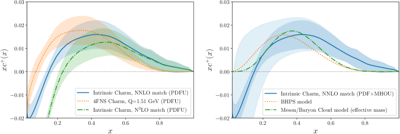
Figure 1: The intrinsic charm PDF and comparison with models. Left: the purely intrinsic (3FNS) result (blue) with PDF uncertainties only, compared to the 4FNS PDF, that includes both an intrinsic and radiative component, at $Q=m_{c}=1.51$ GeV (orange). The purely intrinsic (3FNS) result obtained using N³LO matching is also shown (green). Right: the purely intrinsic (3FNS) final result with total uncertainty (PDF+MHOU), with the PDF uncertainty indicated as a dark shaded band; the predictions from the original BHPS model [1] and from the more recent meson/baryon cloud model [5] are also shown for comparison (dotted and dot-dashed curves respectively).

The intrinsic (3FNS) charm PDF displays a characteristic valence-like structure at large-$x$ peaking at $x\simeq 0.4$. While intrinsic charm is found to be small in absolute terms (it contributes less than 1% to the proton total momentum), it is significantly different from zero. Note that the transformation to the 3FNS has little effect on the peak region, because there is almost no charm radiatively generated at such large values of $x$: in fact, a very similar valence-like peak is already found in the 4FNS calculation.

Because at the charm mass scale the strong coupling $\alpha_{s}$ is rather large, the perturbative expansion converges slowly. In order to estimate the effect of missing higher order uncertainties (MHOU), we have also performed the transformation from the 4FNS NNLO charm PDF determined from the data to the 3FNS (intrinsic) charm PDF at one order higher, namely at N³LO. The result is also shown Fig. 1 (left). Reassuringly, the intrinsic valence-like structure is unchanged. On the other hand, it is clear that for $x\mathrel{\hbox to0.0pt{\lower 4.0pt\hbox{\hskip 1.0pt$\sim$}\hss}\raise 1.0pt\hbox{$<$}}0.2$ perturbative uncertainties become very large. We can estimate the total uncertainty on our determination of intrinsic charm by adding in quadrature the PDF uncertainty and a MHOU estimated from the shift between the result found using NNLO and N³LO matching.

This procedure leads to our final result for intrinsic charm and its total uncertainty, shown in Fig. 1 (right). The intrinsic charm PDF is found to be compatible with zero for $x\mathrel{\hbox to0.0pt{\lower 4.0pt\hbox{\hskip 1.0pt$\sim$}\hss}\raise 1.0pt\hbox{$<$}}0.2$: the negative trend seen in Fig. 1 with PDF uncertainties only becomes compatible with zero upon inclusion of theoretical uncertainties. However, at larger $x$ even with theoretical uncertainties the intrinsic charm PDF differs from zero by about 2.5 standard deviations ($2.5\sigma$) in the peak region. This result is stable upon variations of dataset, methodology (in particular the PDF parametrization basis) and Standard Model parameters (specifically the charm mass), as demonstrated in the Supplementary Information (SI) Sects. C and D.

Our determination of intrinsic charm can be compared to theoretical expectations. Subsequent to the original intrinsic charm model of [1] (BHPS model), a variety of other models were proposed [35, 36, 37, 38, 5], see [2] for a review. Irrespective of their specific details, most models predict a valence-like structure at large $x$ with a maximum located between $x\simeq 0.2$ and $x\simeq 0.5$, and a vanishing intrinsic component for $x\mathrel{\hbox to0.0pt{\lower 4.0pt\hbox{\hskip 1.0pt$\sim$}\hss}\raise 1.0pt\hbox{$<$}}0.1$. In Fig. 1 (right) we compare our result to the original BHPS model and to the more recent meson/baryon cloud model of [5].

As these models predict only the shape of the intrinsic charm distribution, but not its overall normalization, we have normalized them by requiring that they reproduce the same charm momentum fraction as our determination. We find remarkable agreement between the shape of our determination and the model predictions. In particular, we reproduce the presence and location of the large-$x$ valence-like peak structure (with better agreement, of marginal statistical significance, with the meson/baryon cloud calculation), and the vanishing of intrinsic charm at small-$x$. The fraction of the proton momentum carried by charm quarks that we obtain from our analysis, used in this comparison to models, is $\left(0.62\pm 0.28\right)\%$ including PDF uncertainties only (see SI Sect. E for details). However, the uncertainty upon inclusion of MHOU greatly increases, and we obtain $\left(0.62\pm 0.61\right)\%$, due to the contribution from the small-$x$ region, $x\mathrel{\hbox to0.0pt{\lower 4.0pt\hbox{\hskip 1.0pt$\sim$}\hss}\raise 1.0pt\hbox{$<$}}0.2$, where the MHOU is very large, see Fig. 1 (right). Note that in most previous analyses [18] (see SI Sect. F) intrinsic charm models (such as the BHPS model) are fitted to the data, with only the momentum fraction left as a free parameter.

We emphasize that in our analysis the charm PDF is entirely determined by the experimental data included in the PDF determination. The data with the most impact on charm are from recently measured LHC processes, which are both accurate and precise. Since these measurements are made at high scales, the corresponding hard cross-sections can be reliably computed in QCD perturbation theory.

Independent evidence for intrinsic charm is provided by the very recent LHCb measurements of $Z$-boson production in association with charm-tagged jets in the forward region [6], which were not included in our baseline dataset. This process, and specifically the ratio $\mathcal{R}_{j}^{c}$ of charm-tagged jets normalized to flavor-inclusive jets, is directly sensitive to the charm PDF [39], and with LHCb kinematics also in the kinematic region where the intrinsic component is relevant. Following [39, 6], we have evaluated $\mathcal{R}_{j}^{c}$ at NLO [40, 41] (see SI Sect. G for details), both with our default PDFs that include intrinsic charm, and also with an independent PDF determination in which intrinsic charm is constrained to vanish identically, so charm is determined by perturbative matching (see SI Sect. B).

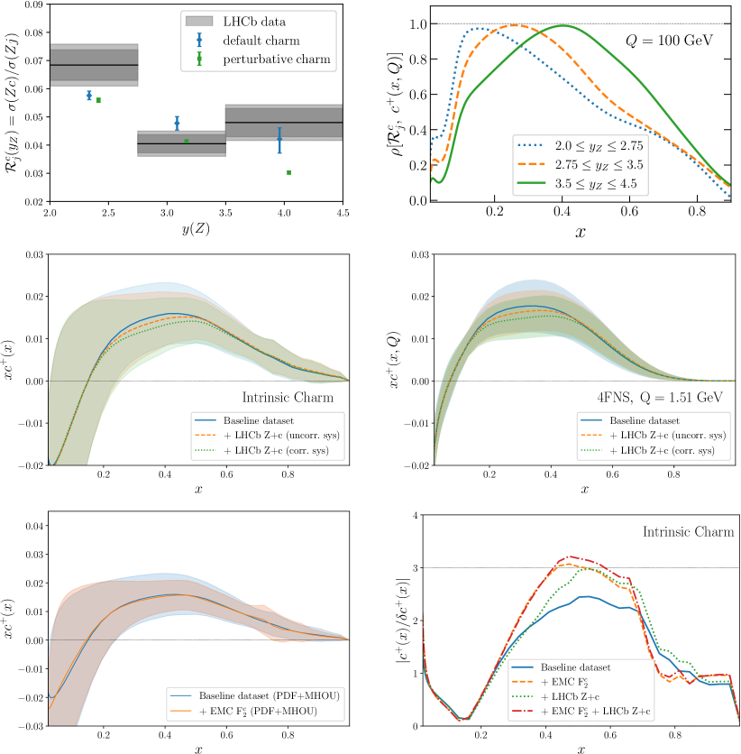
Figure 2: Intrinsic charm and $Z+$charm production at LHCb. Top left: the LHCb measurements of $Z$ boson production in association with charm-tagged jets, $\mathcal{R}_{j}^{c}$, at $\sqrt{s}=13$ TeV, compared with our default prediction which includes an intrinsic charm component, as well as with a variant in which we impose the vanishing of the intrinsic charm component. The thicker (thinner) bands in the LHCb data indicate the statistical (total) uncertainty, while the theory predictions include both PDF and MHO uncertainties. Top right: the correlation coefficient between the charm PDF at $Q=100$ GeV in NNPDF4.0 and the LHCb measurements of $\mathcal{R}_{j}^{c}$ for the three $y_{Z}$ bins. Center: the charm PDF in the 4FNS (right) and the intrinsic (3FNS) charm PDF (left) before and after inclusion of the LHCb $Z$+charm data. Results are shown for both experimental correlation models discussed in the text. Bottom left: the intrinsic charm PDF before and after inclusion of the EMC charm structure function data. Bottom right: the statistical significance of the intrinsic charm PDF in our baseline analysis, compared to the results obtained also including either the LHCb $Z$+charm (with uncorrelated systematics) or the EMC structure function data, or both.

In Fig. 2 (top left) we compare the LHCb measurements of $\mathcal{R}_{j}^{c}$, provided in three bins of the $Z$-boson rapidity $y_{Z}$, with the theoretical predictions based on both our default PDFs as well as the PDF set in which we impose the vanishing of intrinsic charm. In Fig. 2 (top right) we also display the correlation coefficient between the charm PDF at $Q=100$ GeV and the observable $\mathcal{R}_{j}^{c}$, demonstrating how this observable is highly correlated to charm in a localized $x$ region that depends on the rapidity bin. It is clear that our prediction is in excellent agreement with the LHCb measurements, while in the highest rapidity bin, which is highly correlated to the charm PDF in the region of the observed valence peak $x\simeq 0.45$, the prediction obtained by imposing the vanishing of intrinsic charm undershoots the data at the $3\sigma$ level. Hence this measurement provides independent direct evidence in support of our result.

We have also determined the impact of these LHCb $Z$+charm measurements on the charm PDF. Since the experimental covariance matrix is not available, we have considered two limiting scenarios in which the total systematic uncertainty is either completely uncorrelated ($\rho_{\rm sys}=0$) or fully correlated ($\rho_{\rm sys}=1$) between rapidity bins. The charm PDF in the 4FNS before and after inclusion of the LHCb data (with either correlation model), and the intrinsic charm PDF obtained from it, are displayed in Fig. 2 (center left and right respectively). The bands account for both PDF and MHO uncertainties. The results show full consistency: inclusion of the LHCb $\mathcal{R}_{j}^{c}$ data leaves the intrinsic charm PDF unchanged, while moderately reducing the uncertainty on it.

In the past, the main indication for intrinsic charm came from EMC data [42] on deep inelastic scattering with charm in the final state [43]. These data are relatively imprecise, their accuracy has often been questioned, and they were taken at relatively low scales where radiative corrections are large. For these reasons, we have not included them in our baseline analysis. However, it is interesting to assess the impact of their inclusion. Results are shown in Fig. 2 (bottom left), where we display the intrinsic charm PDF before and after inclusion of the EMC data. Just like in the case of the LHCb data we find full consistency: unchanged shape and a moderate reduction of uncertainties.

We can summarize our results through their so-called local statistical significance, namely, the size of the intrinsic charm PDF in units of its total uncertainty. This displayed in Fig. 2 (bottom right) for our default determination of intrinsic charm, as well as after inclusion of either the LHCb $Z$+charm or the EMC data, or both. We find a local significance for intrinsic charm at the $2.5\sigma$ level in the region $0.3\mathrel{\hbox to0.0pt{\lower 4.0pt\hbox{\hskip 1.0pt$\sim$}\hss}\raise 1.0pt\hbox{$<$}}x\mathrel{\hbox to0.0pt{\lower 4.0pt\hbox{\hskip 1.0pt$\sim$}\hss}\raise 1.0pt\hbox{$<$}}0.6$. This is increased to about $3\sigma$ by the inclusion of either the EMC or the LHCb data, and above if they are both included. The similarity of the impact of the EMC and LHCb measurements is especially remarkable in view of the fact that they involve very different physical processes and energies.

In summary, in this work we have presented long-sought evidence for intrinsic charm quarks in the proton. Our findings close a fundamental open question in the understanding of nucleon structure that has been hotly debated by particle and nuclear physicists for the last 40 years. By carefully disentangling the perturbative component, we obtain unambiguous evidence for intrinsic charm, which turns out to be in qualitative agreement with the expectations from model calculations. Our determination of the charm PDF, driven by indirect constraints from the latest high-precision LHC data, is perfectly consistent with direct constraints both from EMC charm production data taken forty years ago, and with very recent $Z$+charm production data in the forward region from LHCb. Combining all data, we find local significance for intrinsic charm in the large-$x$ region just above the $3\sigma$ level. Our results motivate further dedicated studies of intrinsic charm through a wide range of nuclear, particle and astro-particle physics experiments, from the High-Luminosity LHC [44] and the fixed-target programs of LHCb [45] and ALICE [46], to the Electron Ion Collider, AFTER [47], the Forward Physics Facility [48], and neutrino telescopes [49].

Acknowledgments

We thank our colleagues of the NNPDF Collaboration for many illuminating discussions concerning the charm PDF. We are grateful to Johannes Blümlein for communicating Mathematica code with the results of [26, 27, 28, 29, 30, 31, 32, 33, 34], to Jakob Ablinger for assistance in the implementation of the $\mathcal{O}\left(\alpha_{s}^{3}\right)$ calculation of the heavy quark matching conditions, and to Silvia Zanoli for sharing her Mathematica implementation with us. We are grateful to Rhorry Gauld for discussions, assistance and sharing his Pythia8 implementation for the calculation $Z$+charm production. We thank Marco Guzzi and Pavel Nadolsky for discussions concerning intrinsic charm in the CT family of global PDF fits, and Tim Hobbs and Wally Melnitchouk for providing us with their predictions of the meson/baryon cloud model. We are grateful to Tom Boettcher, Philip Ilten, and Michael Williams to assistance with the LHCb $Z$+charm measurements.

Funding information

S. F., J. C.-M., F. H., A. C., and K. K. are supported by the European Research Council under the European Union’s Horizon 2020 research and innovation Programme (grant agreement n.740006). R. D. B. is supported by the U.K. Science and Technology Facility Council (STFC) grant ST/P000630/1. J. R. and G. M. are partially supported by NWO (Dutch Research Council). T. G. is supported by NWO (Dutch Research Council) via an ENW-KLEIN-2 project.

Code and data availability

The analysis presented in this work has been carried out using two open-source software frameworks, NNPDF for the global PDF determination and EKO for the calculation of the 3FNS charm. These codes are publicly available from https://docs.nnpdf.science/ and https://eko.readthedocs.io/ respectively. Both the LHAPDF grids produced in this work and the version of EKO with the respective run cards used are made available from http://nnpdf.mi.infn.it/nnpdf4-0-charm-study/.

Author contributions

As customary in high-energy physics, authors are listed in alphabetical order.

J. C. M. is the main author of the new algorithm used in the NNPDF4.0 PDF determination. A. C., F. H., and G. M. developed the EKO code used to evaluate the 3FNS charm PDF, and specifically G. M. implemented the matching conditions, with the help of K. K. for the implementation of some harmonic sums. T. G. performed the analysis of the LHCb $Z$+charm data. R. D. B. and S. F. designed the general procedure. J. R. coordinated the intrinsic charm determination and S. F. supervised the whole project. J. R.  and S. F. wrote the paper and R. D. B. revised it. All authors discussed the results and their implications.

Methods

The strategy adopted in this work in order to determine the intrinsic charm content of the proton is based on the following observation. The assumption that there is no intrinsic charm amounts to the assumption that all 4FNS PDFs are determined [24] using perturbative matching conditions [25] in terms of 3FNS PDFs that do not include a charm PDF. However, these perturbative matching conditions are actually given by a square matrix that also includes a 3FNS charm PDF. So the assumption of no intrinsic charm amounts to the assumption that if the 4FNS PDFs are transformed back to the 3FNS, the 3FNS charm PDF is found to vanish. Hence, intrinsic charm is by definition the deviation from zero of the 3FNS charm PDF [21]. Note that whereas the 3FNS charm PDF is purely intrinsic, while the 4FNS charm PDF includes both an intrinsic and a perturbative radiative component, the 4FNS intrinsic component is not equal to the 3FNS charm PDF, since matching conditions reshuffle all PDFs among each other.

Intrinsic charm can then be determined through the following two steps, summarized in Fig. 3. First, all the PDFs, including the charm PDF, are parametrized in the 4FNS at an input scale $Q_{0}$ and evolved using NNLO perturbative QCD to $Q\not=Q_{0}$. These evolved PDFs can be used to compute physical cross-sections, also at NNLO, which then are compared to a global dataset of experimental measurements. The result of this first step in our procedure is a Monte Carlo (MC) representation of the probability distribution for the 4FNS PDFs at the input parametrization scale $Q_{0}$.

Next, this 4FNS charm PDF is transformed to the 3FNS at some scale matching scale $Q_{c}$. Note that the choice of both $Q_{0}$ and $Q_{c}$ are immaterial. The former because perturbative evolution is invertible, so results for the PDFs do not depend on the choice of parametrization scale $Q_{0}$. The latter because the 3FNS charm is scale independent, so it does not depend on the value of $Q_{c}$. Both statements of course hold up to fixed perturbative accuracy, and are violated by MHO corrections. In practice, we parametrize PDFs at the scale $Q_{0}=$ 1.65 GeV and perform the inversion at a scale chosen equal to the charm mass $Q_{c}=m_{c}=1.51$ GeV.

The scale-independent 3FNS charm PDF is then the sought-for intrinsic charm.

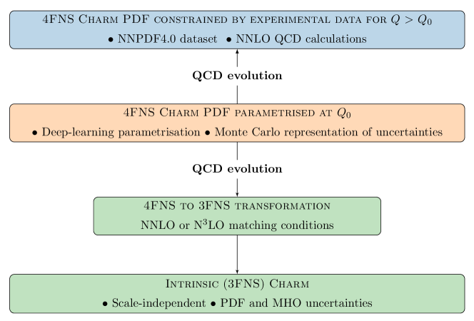
Figure 3: The 4FNS charm PDF is parametrized at $Q_{0}$ and evolved to all $Q$, where it is constrained by the NNPDF4.0 global dataset. Subsequently, it is transformed to the 3FNS where (if nonzero) it provides the intrinsic charm component.

Global QCD analysis.

The 4FNS charm PDF and its associated uncertainties is determined by means of a global QCD analysis within the NNPDF4.0 framework. All PDFs, including the charm PDF, are parametrized at $Q_{0}=1.65$ GeV in a model-independent manner using a neural network, which is fitted to data using supervised machine learning techniques. The Monte Carlo replica method is deployed to ensure a faithful uncertainty estimate. Specifically, we express the 4FNS total charm PDF ($c^{+}=c+\bar{c}$) in terms of the output neurons associated to the quark singlet $\Sigma$ and non-singlet $T_{15}$ distributions, see Sect. 3.1 of [3], as

$$xc^{+}(x,Q_{0};{\boldsymbol{\theta}})=\left(x^{\alpha_{\Sigma}}(1-x)^{\beta_{\Sigma}}{\rm NN}_{\Sigma}(x,{\boldsymbol{\theta}})-x^{\alpha_{T_{15}}}(1-x)^{\beta_{T_{15}}}{\rm NN}_{T_{15}}(x,{\boldsymbol{\theta}})\right)/4\,,$$ (1)

where ${\rm NN}_{i}(x,{\boldsymbol{\theta}})$ is the $i$-th output neuron of a neural network with input $x$ and parameters ${\boldsymbol{\theta}}$, and $\left(\alpha_{i},\beta_{i}\right)$ are preprocessing exponents. A crucial feature of Eq. (1) is that no ad hoc specific model assumptions are used: the shape and size of $xc^{+}(x,Q_{0})$ are entirely determined from experimental data. Hence, our determination of the 4FNS fitted charm PDF, and thus of the intrinsic charm, is unbiased.

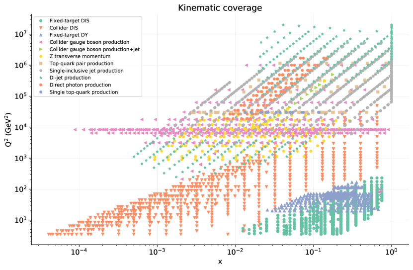
Figure 4: The kinematic coverage in the $(x,Q)$ plane covered by the 4618 cross-sections used for the determination of the charm PDF in the present work. These cross-sections have been classified into the main different types of processes entering the global analysis.

The neural network parameters ${\boldsymbol{\theta}}$ in Eq. (1) are determined by fitting an extensive global dataset that consists of 4618 cross-sections from a wide range of different processes, measured over the years in a variety of fixed-target and collider experiments (see [3] for a complete list). Fig. 4 displays the kinematic coverage in the $(x,Q)$ plane covered by these cross-sections, where $Q$ is the scale, and $x$ is the parton momentum fraction that correspond to leading-order kinematics. Many of these processes provide direct or indirect sensitivity to the charm content of the proton. Particularly important constraints come from $W$ and $Z$ production from ATLAS, CMS, and LHCb as well as from neutral and charged current deep-inelastic scattering (DIS) structure functions from HERA. The 4FNS PDFs at the input scale $Q_{0}$ are related to experimental measurements at $Q\not=Q_{0}$ by means of NNLO QCD calculations, including the FONLL-C general-mass scheme for DIS [20] generalized to allow for fitted charm [4].

We have verified (see SI Sects. C and D) that the determination of 4FNS charm PDF Eq. (1) and the ensuing 3FNS intrinsic charm PDF are stable upon variations of methodology (PDF parametrization basis), input dataset, and values of Standard Model parameters (the charm mass). We have also studied the stability of our results upon replacing the current NNPDF4.0 methodology [3] with the previous NNPDF3.1 methodology [50]. It turns out that results are perfectly consistent. Indeed, the old methodology leads to somewhat larger uncertainties, corresponding to a moderate reduction of the local statistical significance for intrinsic charm, and to a central value which is within the smaller error band of our current result.

A determination in which the vanishing of intrinsic charm is imposed has also been performed. In this case, the fit quality significantly deteriorates: the values of the $\chi^{2}$ per data point of 1.162, 1.26, and 1.22 for total, Drell-Yan, and neutral-current DIS data respectively, found when fitting charm, are increased to 1.198, 1.31, 1.28 when the vanishing of intrinsic charm is imposed. The absolute worsening of the total $\chi^{2}$ when the vanishing of intrinsic charm is imposed is therefore of 166 units, corresponding to a $2\sigma$ effects in units of $\sigma_{\chi^{2}}=\sqrt{2n_{\rm dat}}$.

Calculation of the 3FNS charm PDF.

The Monte Carlo representation of the probability distribution associated to the 4FNS charm PDF determined by the global analysis contains an intrinsic component mixed with a perturbatively generated contribution, with the latter becoming larger in the $x\mathrel{\hbox to0.0pt{\lower 4.0pt\hbox{\hskip 1.0pt$\sim$}\hss}\raise 1.0pt\hbox{$<$}}0.1$ region as the scale $Q$ is increased. In order to extract the intrinsic component, we transform PDFs to the 3FNS at the scale $Q_{c}=m_{c}=1.51$ GeV using EKO, a novel Python open source PDF evolution framework (see SI Sect. A). In its current implementation, EKO performs QCD evolution of PDFs to any scale up to NNLO. For the sake of the current analysis, N³LO matching conditions have also been implemented, by using the results of [26, 27, 28, 29, 30, 31, 32, 33, 34] for $\mathcal{O}(\alpha_{s}^{3})$ operator matrix elements  so that the direct and inverse transformations from the 3FNS to the 4FNS can be performed at one order higher. The N³LO contributions to the matching conditions are a subset of the full N³LO terms that would be required to perform a PDF determination to one higher perturbative order, and would also include currently unknown N³LO contributions to QCD evolution. Therefore, our results have NNLO accuracy and we can only use the N³LO contributions to the $\mathcal{O}(\alpha_{s}^{3})$ corrections to the heavy quark matching matching conditions as a way to estimate the the size of the missing higher orders. Indeed, these corrections have a very significant impact on the perturbatively generated component, see SI Sect. B. They become large for $x\mathrel{\hbox to0.0pt{\lower 4.0pt\hbox{\hskip 1.0pt$\sim$}\hss}\raise 1.0pt\hbox{$<$}}0.1$, which coincides with the region dominated by the perturbative component of the charm PDF, and are relatively small for the valence region where intrinsic charm dominates.

$Z$ production in association with charm-tagged jets.

The production of $Z$ bosons in association with charm-tagged jets (or alternatively, with identified $D$ mesons) at the LHC is directly sensitive to the charm content of the proton via the dominant $gc\to Zc$ partonic scattering process. Measurements of this process at the forward rapidities covered by the LHCb acceptance provide access to the large-$x$ region where the intrinsic contribution is expected to dominate. This is in contrast with the corresponding measurements from ATLAS and CMS, which only become sensitive to intrinsic charm at rather larger values of $p_{T}^{Z}$ than those currently accessible experimentally.

We have obtained theoretical predictions for $Z$+charm production at LHCb with NNPDF4.0, based on NLO QCD calculations using POWHEG-BOX interfaced to Pythia8 with the Monash 2013 tune for showering, hadronization, and underlying event. Acceptance requirements and event selection follow the LHCb analysis, where in particular charm jets are defined as those anti-$k_{T}$ $R=0.5$ jets containing a reconstructed charmed hadron. The ratio between $c$-tagged and untagged $Z$+jet events can then be compared with the LHCb measurements

$$\mathcal{R}_{j}^{c}(y_{Z})\equiv{{N(c~{}{\rm tagged~{}jets};y_{Z})}\over{N({\rm jets};y_{Z})}}={{\sigma(pp\to Z+{\rm charm~{}jet};y_{Z})}\over{\sigma(pp\to Z+{\rm jet};y_{Z})}}\,,$$ (2)

as a function of the $Z$ boson rapidity $y_{Z}$ (see SI Sect. G for details). The more forward the rapidity $y_{Z}$, the higher the values of the charm momentum $x$ being probed. Furthermore, we have also included the LHCb measurements in the global PDF determination by means of the Bayesian reweighting (see SI Sect. G).

Supplementary Information

Evidence for intrinsic charm quarks in the proton

The NNPDF Collaboration:
Richard D. Ball,¹ Alessandro Candido,² Juan Cruz-Martinez,² Stefano Forte,² Tommaso Giani,^3,4
Felix Hekhorn,² Kirill Kudashkin,² Giacomo Magni,^3,4 and Juan Rojo^3,4

¹The Higgs Centre for Theoretical Physics, University of Edinburgh,
JCMB, KB, Mayfield Rd, Edinburgh EH9 3JZ, Scotland
 ²Tif Lab, Dipartimento di Fisica, Università di Milano and
INFN, Sezione di Milano, Via Celoria 16, I-20133 Milano, Italy
 ³Department of Physics and Astronomy, Vrije Universiteit, NL-1081 HV Amsterdam
 ⁴Nikhef Theory Group, Science Park 105, 1098 XG Amsterdam, The Netherlands

Contents

1. A The EKO evolution framework
2. B The perturbative charm PDF
3. C Stability of the 4FNS charm PDF
4. D Stability of the 3FNS charm calculation
5. E The charm momentum fraction
6. F Comparison with CT14IC
7. G $Z$+charm production in the forward region
8. H Parton luminosities

Appendix A The EKO evolution framework

A crucial ingredient in the derivation of our results is the determination of the 3FNS intrinsic charm PDF starting from the 4FNS, which requires the inversion of the matching conditions implementing the 3FNS to the 4FNS transformation. This inversion is not available in the open-source NNPDF code NNPDF:2021uiq and it is performed here by means of a novel code for QCD evolution, EKO (Evolution Kernel Operators), that we use to take the PDF set determined at the reference scale $Q_{0}$ and evolve it to a matching scale $Q_{c}$ where it is transformed to the 3FNS. Here we provide a brief summary of EKO, some details of the way the direct and inverse matching conditions are implemented, and some benchmarks between EKO and other existing QCD evolution codes, including the APFEL Bertone:2013vaa evolution code that is used by the NNPDF code. EKO is written in Python and is available open source from its GitHub repository

https://github.com/N3PDF/eko

A more detailed description of the code can be found in its online documentation

https://eko.readthedocs.io/en/latest/

as well as in a dedicated publication Candido:2022tld.

The scale dependence of PDFs in QCD is determined by solving a set of coupled integro-differential equations (evolution equations) in two variables $x$ (momentum fraction) and $Q$ (scale) on which PDFs depend. Two families of approaches are commonly used in order to this purpose. One possibility is to treat the (integral) dependence on $x$ of the PDFs and evolution kernels by sampling it on a grid of points. This is the strategy adopted by, among others, the APFEL Bertone:2013vaa, HOPPET Salam:2008qg, and QCDNUM Botje:2010ay evolution codes. An alternative possibility is to perform an integral transform (Mellin transform) with respect to $x$ thereby turning the integro-differential equations into coupled ordinary differential equations. These can then be solved analytically, but the integral transform has to be inverted numerically to arrive at a final result. This approach is adopted by PEGASUS pegasus as well as by the internal PDF evolution code FastKernel used in earlier NNPDF analyses and described in DelDebbio:2007ee,Ball:2008by,Ball:2010de. One limitation of PEGASUS is that it requires the analytic computation of the Mellin transforms of the PDFs, which is generally not possible, specifically if PDFs are parametrized as neural networks.

This restriction is bypassed in FastKernel by transforming only the evolution kernel (i.e. the evolution operator, solution of differential equations, evaluated on a given interpolation basis), which can be then convoluted with the $x$-space PDFs at the input evolution scale $Q_{0}$. Following a similar strategy, EKO solves evolution equations in Mellin space and then produces PDF-independent evolution kernel operators (EKO) which can be convoluted with input PDFs. Variable flavor number scheme evolution (VFNS) is implemented in EKO, with the possibility of freely choosing the value of the matching scales $Q_{h}$ between the $N$-flavor number scheme (NFNS) in which heavy quark $h$ is not included in QCD evolution, and the $(N+1)$-flavor number scheme in which it is included. Schematically, for evolution between $Q_{0}$ and $Q_{1}$ if no matching scales are crossed $\left(Q_{h}^{2}<Q_{0}^{2},Q_{1}^{2}<Q_{h^{\prime}}^{2}\right)$ one has:

$${\mathbf{f}}^{(n_{f})}(Q^{2}_{1})={\mathbf{E}}^{(n_{f})}(Q^{2}_{1}\leftarrow Q^{2}_{0})\otimes{\mathbf{f}}^{(n_{f})}(Q^{2}_{0})\,,$$ (A.1)

where ${\mathbf{E}}^{(n_{f})}$ is the NFNS EKO, and $\otimes$ is the Mellin convolution operation. Note that EKO can perform both “forward” ($Q_{0}<Q_{1}$) and “backward” ($Q_{1}<Q_{0}$) evolution. Bold quantities indicate either vectors or matrices in the $(2n_{f}+1)$-dimensional flavor space. If instead a single matching scale $Q_{h}$ is crossed, assuming for definiteness $Q_{0}<Q_{1}$, $Q_{h^{\prime}}^{2}<Q_{0}^{2}<Q_{h}^{2}<Q_{1}^{2}<Q_{h^{\prime\prime}}^{2}$, one has

$${\mathbf{f}}^{(n_{f}+1)}(Q^{2}_{1})=\left[{\mathbf{E}}^{(n_{f}+1)}(Q^{2}_{1}\leftarrow Q_{h}^{2}){\mathbf{A}}^{(n_{f})}(Q_{h}^{2}){\mathbf{E}}^{(n_{f})}(Q_{h}^{2}\leftarrow Q^{2}_{0})\right]\otimes{\mathbf{f}}^{(n_{f})}(Q^{2}_{0})\,,$$ (A.2)

where $\mathbf{A}^{(n_{f})}(Q_{h}^{2})$ is the scheme transformation between the NFNS and (N+1)FNS, given as a perturbatively computable series expansion in $\alpha_{s}$. The quantity in square parenthesis is evaluated in Mellin space and then transformed to $x$-space. This procedure can be extended to the case in which more than one threshold is crossed. Also, the scales $Q_{0}$ and $Q_{1}$ can be ordered in any way, because both direct and inverse scheme transformations are implemented in EKO. Furthermore, the inverse scheme change is implemented both perturbatively (i.e. as a series expansion in $\alpha_{s}$ to the same accuracy as the direct scheme change) or exactly (i.e. as the numerical inverse, completely equivalent to the analytic one within the numeral accuracy of the rest of the calculation).

If the heavy quark $h$ has no intrinsic component, then below $Q_{h}$ its PDF is identically zero, and above $Q_{h}$ it is determined by $\mathbf{A}^{(n_{f})}(Q_{h}^{2})$. If it does have an intrinsic component, then below $Q_{h}$ its PDF is scale-independent, but nonzero. While EKO is currently an NNLO code, on top of the standard [25] NNLO scheme change for this work an N³LO scheme change has been implemented, based on recent higher-order computations of the relevant operator matrix elements [26, 27, 28, 29, 30, 31, 34, 32, 33] and the work of zanoli.

The EKO implementation of QCD evolution has been benchmarked against the Les Houches PDF evolution benchmarks Dittmar:2005ed,Giele:2002hx and with APFEL and PEGASUS, finding excellent agreement beyond the per-mille level. The implementation of the matching conditions has been benchmarked up to N³LO against the independent Mathematica-based calculation presented in zanoli finding also good agreement. To illustrate some of these benchmarks, Fig. A.1 displays the absolute and relative difference between EKO, APFEL, and PEGASUS for NNLO VFNS evolution carried out following the settings of Dittmar:2005ed,Giele:2002hx. A toy PDF set at $Q_{0}=\sqrt{2}$ GeV is evolved up to $Q=100$ GeV for equal values of the factorization and renormalization scales, $Q_{f}=Q_{r}=Q$. We show as representative results those corresponding to the total valence quark $V$ and the quark singlet $\Sigma$ distributions. Excellent agreement is found, in particular with PEGASUS which also perform QCD evolution in Mellin space, with relatively differences at most at the $\mathcal{O}\left(10^{-4}\right)$ level. A similar level of agreement is found for the gluon and for the other quark PDF combinations.

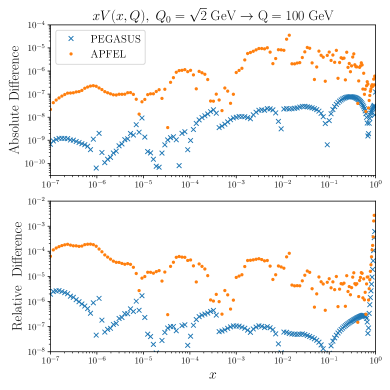
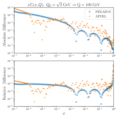
Figure A.1: Absolute (upper) and relative (bottom) differences between the outcome of NNLO QCD evolution as implemented in EKO and the corresponding results from APFEL and PEGASUS. We adopt the settings of the Les Houches PDF evolution benchmarks: we consider VFNS evolution from $Q_{0}=\sqrt{2}$ GeV up to $Q=100$ GeV, and we show results for the total valence quark distribution $V$ (left) and the quark singlet distribution $\Sigma$ (right).

Appendix B The perturbative charm PDF

In the absence of intrinsic charm, the charm PDF is fully determined by perturbative matching conditions, i.e. by the matrix $\mathbf{A}^{(n_{f})}(Q_{c}^{2})$ in Eq. (A.2). We will denote the charm PDF thus obtained “perturbative charm PDF”, for short. The PDF uncertainty on the perturbative charm PDF is directly related to that of the light quarks and especially the gluon, and is typically much smaller than the uncertainty on our default charm PDF, that includes intrinsic charm. Here and in the following we will refer to our final result, as shown in Fig. 1 (right) as “default”. It should be noticed that the matching conditions for charm are nontrivial starting at NNLO: at NLO the perturbative charm PDF vanishes at threshold. Hence, having implemented in EKO also the N³LO matching conditions, we are able to assess the MHOU of the perturbative charm at the matching scale $Q_{c}$, by comparing results obtained at the first two nonvanishing perturbative orders.

As already mentioned, see also Fig. 2 (top left) in the main manuscript, we have constructed a PDF set with perturbative charm, in which the full PDF determination from the global dataset leading to the NNPDF4.0 PDF set is repeated, but now with the assumption of vanishing intrinsic charm, i.e. with a perturbative charm PDF. This perturbative charm PDF is compared to our default result in Fig. B.1 (left), where the 4FNS perturbative charm PDF at scale $Q_{c}=m_{c}$ obtained using either NNLO or N³LO under the assumption of no intrinsic charm are shown, together with our result allowing for intrinsic charm. It is clear that while on the one hand, the PDF uncertainty on the perturbative charm PDF is indeed tiny, on the other hand the difference between the result for perturbative charm obtained using NNLO or N³LO matching is large, and in fact larger at small $x$ than the difference between perturbative charm and our default (intrinsic) result.

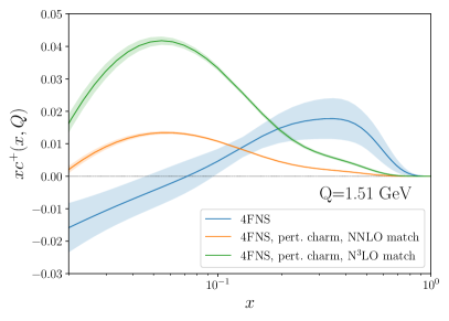
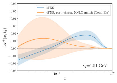
Figure B.1: Left: the perturbative charm PDF at $Q=1.51$ GeV obtained from NNLO PDFs using NNLO and N³LO matching conditions. Right: the NNLO perturbative charm PDF including the MHOU computed as the difference between NNLO and N³LO matching. In both plots our default (intrinsic) charm PDF is also shown for comparison.

In the same manner as we used the difference between the results obtained from inversion of NNLO and N³LO matching as an estimate of the MHOU on intrinsic charm, we may use the difference between the 4FNS perturbative charm obtained from NNLO and N³LO matching as an estimate of the MHOU on perturbative charm at the scale $Q_{c}$. The total uncertainty is found by adding this in quadrature to the PDF uncertainty (which however in practice is negligible). The result is shown in Fig. B.1 (right). Within this total uncertainty there is now good agreement between our intrinsic charm result and perturbative charm for all $x\mathrel{\hbox to0.0pt{\lower 4.0pt\hbox{\hskip 1.0pt$\sim$}\hss}\raise 1.0pt\hbox{$<$}}0.2$. On the other hand, there is a clear deviation for larger $x$. We may view the difference between the 4FNS default result and the 4FNS perturbative charm as the intrinsic component in the 4FNS, and indeed it is clear from Fig. B.1 that the 4FNS intrinsic component is sizable and positive at large $x$. This is of course consistent with our main finding that we only see evidence of intrinsic charm for large $x\mathrel{\hbox to0.0pt{\lower 4.0pt\hbox{\hskip 1.0pt$\sim$}\hss}\raise 1.0pt\hbox{$>$}}0.2$, while for smaller $x$ our result for the charm PDF is compatible with zero, as demonstrated by Fig. 1 (right) in the main manuscript.

Appendix C Stability of the 4FNS charm PDF

The main input to our determination of intrinsic charm is the 4FNS charm PDF extracted from high-energy data. While this determination comes with an uncertainty estimate, it is important to verify that this adequately reflects the various sources of uncertainty, and that there are no further sources of uncertainty that may be unaccounted for. To this purpose, here we assess the stability of our results first, upon the choice of underlying dataset, next upon changes in methodology, and finally, upon variation of standard model parameters. In each case we verify stability upon the most important possible source of instability: respectively, the use of collider vs. fixed target and deep-inelastic vs. hadronic data (dataset); the choice of parametrization basis (methodology); and the value of the charm quark mass (standard model parameters). As a final consistency check, we compare our result with that which we would have obtained by using the same input dataset, but the previous NNPDF3.1 fitting methodology. Because we are interested in intrinsic charm, in all comparisons we focus on the large-$x$ region in which the intrinsic valence-like peak is found. In this section, the 4FNS charm PDF is displayed at the scale $Q=1.65$ GeV so that results for all fit variants, including those with with different $m_{c}$ values, can be shown at a common scale.

Dependence on the choice of dataset.

We now study the stability of the 4FNS charm determination upon variation of the underlying data, which also allows us to identify the datasets or groups of processes that provide the leading constraints on intrinsic charm. To this purpose, we have repeated our PDF determination using a variety of subsets of the global dataset used for our default determination. Results are shown in Fig. C.1, where we compare the result using the baseline dataset to determinations performed by adding to the baseline the EMC charm structure function data (already discussed in the main text); by only including DIS data; by only including collider data (HERA, Tevatron and LHC); and by removing the LHCb $W$ and $Z$ production data.

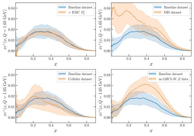
Figure C.1: The dependence of the 4FNS charm PDF at $Q=1.65$ GeV on the input dataset. We compare the baseline result with that obtained by also including EMC $F_{2}^{c}$ data (top left), only including DIS data (top right), only including collider data (bottom left) and removing LHCb gauge boson production data (bottom right).

As already noted in the main text in the case of the 3FNS result, we find that the extra information provided by the EMC $F_{2}^{c}$ data is subdominant in comparison to that from the global dataset. The result is stable and only a moderate uncertainty reduction at the peak is observed. It is interesting to contrast this with the previous NNPDF study [22], in which the global fit provided only very loose constraints on the charm PDF, which was then determined mostly by the EMC data. Indeed, a DIS-only fit (for which most data were already available at the time of the previous determination) determines charm with very large uncertainties. On the other hand, both the central value and uncertainty found in the collider-only fit are quite similar to the baseline result. This shows that the dominant constraint is now coming from collider, and specifically hadron collider data (indeed, as we have seen constraints from DIS data are quite loose). Among these, LHCb data (which are taken at large rapidity and thus impact PDFs at large and small $x$) are especially important, as demonstrated by the increase in uncertainty when they are removed.

In all these determinations, the charm PDF at $x\simeq 0.4$ remains consistently nonzero and positive, thus emphasizing the stability of our results.

Dependence on the parametrization basis.

Among the various methodological choices, a possibly critical one is the choice of basis functions. Specifically, in our default analysis, the output of the neural network does not provide the individual quark flavor and antiflavor PDFs, but rather linear combinations corresponding to the so-called evolution basis [3]. Indeed, our charm PDF is given in Eq. (1) as the linear combination of the two basis PDFs $\Sigma$ and $T_{15}$. One may thus ask whether this choice may influence the final results for individual quark flavors, specifically charm. Given that physical results are basis independent, the outcome of a PDF determination should not depend on the basis choice.

In order to check this, we have repeated the PDF determination, but now using the flavor basis, see Sect. 3.1 of [3], in which each of the neural network output neurons now correspond to individual quark flavors, so in particular, instead of Eq. (1), one has

$$xc^{+}(x,Q_{0};{\boldsymbol{\theta}})=(1-x)^{\beta_{c^{+}}}{\rm NN}_{c^{+}}(x,{\boldsymbol{\theta}})\,,$$ (C.1)

where ${\rm NN}_{c^{+}}(x,{\boldsymbol{\theta}})$ indicates the value of the output neuron associated to the charm PDF $c^{+}$. The 4FNS charm PDFs determined using either basis are compared in Fig. C.2 at $Q=1.65$ GeV. We find excellent consistency, and in particular the valence-like structure at high-$x$ is independent of the choice of parametrization basis.

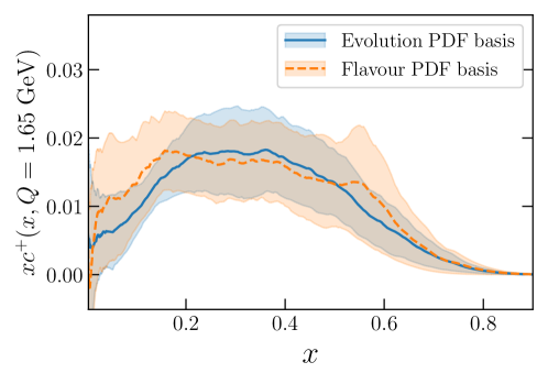
Figure C.2: The default 4FNS charm PDF at $Q=1.65$ GeV compared to a result obtained by parametrizing PDFs in the flavor basis instead of the evolution basis.

Dependence on the charm mass.

The kinematic threshold for producing charm perturbatively depends on the value of the charm mass. Therefore the perturbative contribution to the 4FNS charm PDF, and thus the whole charm PDF if one assumes perturbative charm, depends strongly on the value of the charm mass. On the other hand, the intrinsic charm PDF is of nonperturbative origin, so it should be essentially independent of the numerical value of the charm mass that is used in perturbative computations employed in its determination (though it will of course depend on the true underlying physical value of the charm mass).

In order to study this mass dependence, we have repeated our determination using different values for the charm mass. The definition of the charm mass which is relevant for kinematic thresholds is the pole mass, for which we adopt the value recommended by the Higgs cross-section working group deFlorian:2016spz based on the study of Bauer:2004ve, namely $m_{c}=1.51\pm 0.13$ GeV. Results are shown in Fig. C.3, where our default charm PDF determination with $m_{c}=1.51$ GeV is repeated with $m_{c}=1.38$ GeV and $m_{c}=1.64$ GeV. In order to understand these results note that this is the 4FNS PDF, so it includes both a nonperturbative and a perturbative component. The latter is strongly dependent on the charm mass, but of course the data correspond to the unique true value of the mass and the mass dependence of the perturbative component is present only due to our ignorance of the actual true value. When determining the PDF from the data, as we do, we expect this spurious dependence to be to some extent reabsorbed into the fitted PDF. So we expect results to display a moderate dependence on the charm mass — full independence should hold for the intrinsic (3FNS) PDF and will be investigated in SI Sect. D.

In Fig. C.4 the same result is shown, but now for the perturbative charm PDF discussed in SI Sect. B, so the charm PDF is of purely perturbative origin and fully determined by the strongly mass-dependent matching condition. This dependence is clearly seen in the plots. Furthermore, comparison with Fig. C.3 shows that indeed this spurious dependence is partly reabsorbed in the fit when the charm PDF is determined from the data, so that the residual mass dependence is moderate. In particular, the large-$x$ valence peak, which is dominated by the intrinsic component, is very stable.

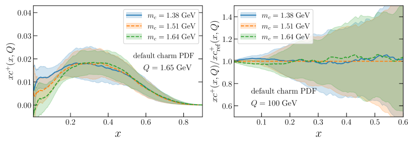
Figure C.3: The 4FNS charm PDF determined using three different values of the charm mass. The absolute result (left) is shown at $Q=1.65$ GeV, while the ratio to the default value $m_{c}=1.51$ GeV (right) used elsewhere in this paper is shown at $Q=100$ GeV.

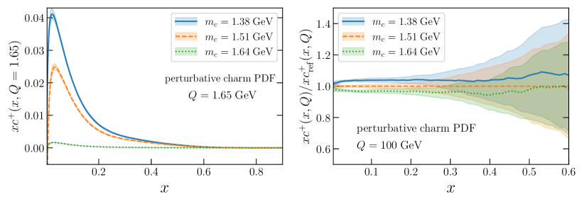
Figure C.4: The same as Fig. C.3 but now for the perturbative charm PDF.

Comparison with NNPDF3.1.

Fig. C.5 compares the baseline determination of the 4FNS charm PDF based on NNPDF4.0 with that obtained from the same input dataset but using instead the NNPDF3.1 fitting methodology and related settings such those related to positivity and integrability. Results are fully consistent between the two methodologies, with our default determination exhibiting reduced uncertainties due to the various improvements implemented in the NNPDF4.0 analysis framework.

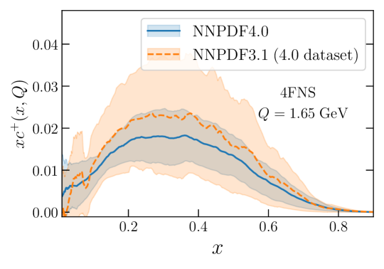
Figure C.5: Same as Fig. C.2, comparing the baseline determination of the 4FNS charm PDF, based on NNPDF4.0, with that obtained from the same dataset using the NNPDF3.1 fitting methodology.

Appendix D Stability of the 3FNS charm calculation

We now repeat the stability and uncertainty study of the previous section, but for our final result, namely the intrinsic charm PDF. The main difference to be kept in mind is that the uncertainty now also includes the dominant MHOU, due to the matching condition required in order to determine the 3FNS PDF from the 4FNS result. In order to get a complete picture, we now add a further set of dataset variations.

Dependence on the input dataset.

Fig. D.1 displays the dataset variations shown in Fig. C.1, now for the intrinsic (3FNS) charm PDF, but with the total uncertainty now being the sum in quadrature of the PDF and MHO uncertainties, with the latter determined as the difference between results obtained using NNLO and N³LO matching. Additionally, we also performed a few extra dataset variations: a fit without any $W,Z$ production data from ATLAS and CMS, a fit without jet data, a fit without $Z$ $p_{T}$ measurements, and a fit without HERA structure function data. Note that the collider-only dataset includes both HERA electron-proton collider data and Tevatron and LHC hadron collider data, but not fixed-target deep-inelastic scattering and Drell-Yan production data.

Results are qualitatively very similar to those seen in the 4FNS, a consequence of the fact that we are focusing on the large-$x$ region where the effect of the matching is moderate, though now the presence of a valence-like peak in all determinations is even clearer, specifically for the DIS-only fit where it was less pronounced in the 4FNS. Note however that the DIS-only determination exhibits larger uncertainties (up to factor 2) and point-by-point fluctuations, and is dominated by relatively old fixed-target measurements. Comparison of all the dataset variations shows that, in terms of their impact on intrinsic charm, hadron collider data are generally more important that deep-inelastic data, that among the former the LHCb inclusive $W,Z$ data are playing a dominant role, and that jet observables also play a non-negligible role.

It should be stressed that the agreement between results found using DIS data and hadron collider data is highly nontrivial, since in the region relevant for intrinsic charm these determinations are based on disjoint datasets and are affected by very different theoretical and experimental uncertainties: in particular, potential higher-twist effects in the DIS observables are highly suppressed for collider observables. this respect, a DIS-only determination of intrinsic charm is potentially affected by sources of theory uncertainties, such as higher twists, which are not accounted for in global PDF determinations.

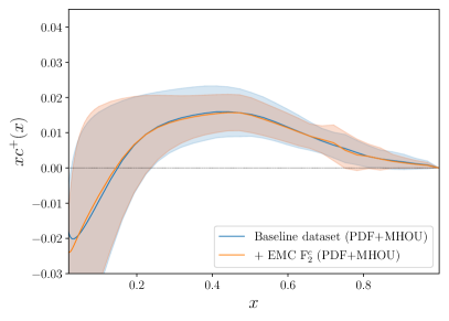
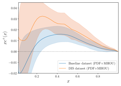
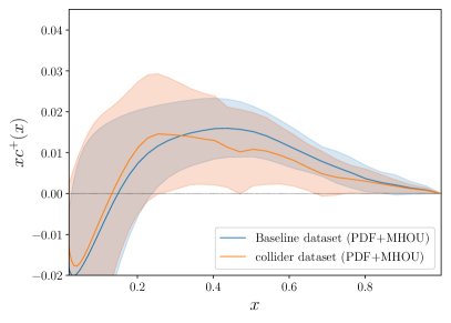
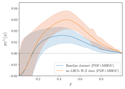
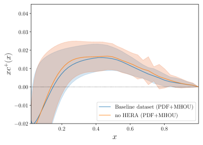
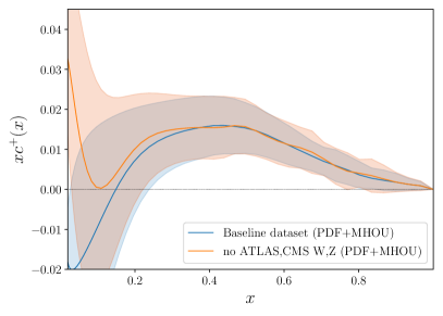
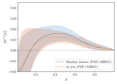
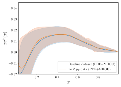
Figure D.1: Same as Fig. C.1 for the intrinsic charm (3FNS) PDF (top four plots), now also including four additional dataset variations: no ATLAS and CMS $W,Z$ production data (third row left), no jet data (third row right), no $Z$ $p_{T}$ measurements (bottom row left), no HERA DIS data (bottom row right). The error band indicates the PDF uncertainties combined in quadrature with the MHOUs.

We conclude that the characteristic valence-like peak structure at large-$x$ predicted by non-perturbative intrinsic charm models (Fig. 1 in the main manuscript) is always present even under very significant changes of the dataset.

Dependence on the parametrization basis.

Fig. D.2 displays the comparison between the intrinsic charm PDF determined with the default evolution basis choice, and the flavor basis. Complete consistency of central values is found, with somewhat larger uncertainties in the case of the flavor basis, due to the more challenging fitting environment in this basis (see the discussion in [3]).

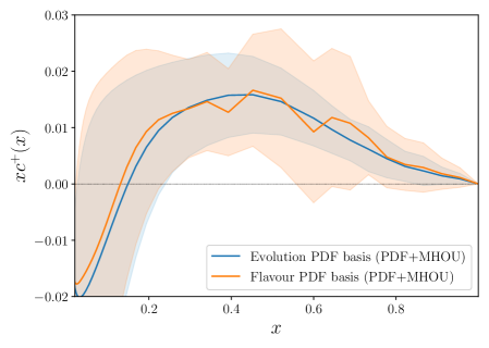
Figure D.2: Same as Fig. C.2 for the intrinsic (3FNS) charm.

Dependence on the charm mass value.

The study of the charm mass dependence is particularly interesting, because the intrinsic component should be independent of it, hence the residual dependence seen in Fig. C.3 in the 4FNS, due to the mass dependence of the perturbative component that could not be reabsorbed in the fitting, should no longer be present. Results are shown in Fig. D.3, and it is apparent that indeed the dependence on the charm mass has all but disappeared.

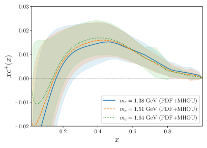
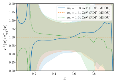
Figure D.3: Same as Fig. C.3, now for the intrinsic (3FNS) charm PDF. Note that the intrinsic charm PDF is scale independent.

Appendix E The charm momentum fraction

The fraction of the proton momentum carried by charm quarks is given by

$$\left[c\right]=\int_{0}^{1}dx\,xc^{+}(x,Q^{2})\,.$$ (E.1)

Model predictions, as mentioned, are typically provided up to an overall normalization, which in turn determines the charm momentum fraction. Consequently, the momentum fraction is often cited as a characteristic parameter of intrinsic charm. It should however be borne in mind that, even in the absence of intrinsic charm, this charm momentum fraction is nonzero due to the perturbative contribution.

In Table E.1 we indicate the values of the charm momentum fraction in the 3FNS for our default charm determination and in the 4FNS (at $Q=1.65$ GeV) both for the default result and for perturbative charm PDF (see SI Sect. B). We provide results for three different values of the charm mass $m_{c}$ and indicate separately the PDF and the MHO uncertainties. The 3FNS result is scale-independent, it corresponds to the momentum fraction carried by intrinsic charm, and it vanishes identically by assumption in the perturbative charm case. The 4FNS result corresponds to the scale-dependent momentum fraction that combines the intrinsic and perturbative contribution, while of course it contains only the perturbative contribution in the case of perturbative charm. As discussed in SI Sect. B, the large uncertainty associated to higher order corrections to the matching conditions affects the 3FNS result (intrinsic charm) in the default case, in which the charm PDF is determined from data in the 4FNS scheme, while it affects the 4FNS result for perturbative charm, that is determined assuming the vanishing of the 3FNS result.

For our default determination, the charm momentum fraction in the 4FNS at low scale differs from zero at the $3\sigma$ level. However, it is not possible to tell whether this is of perturbative or intrinsic origin, because, due to the large MHOU in the matching condition, the intrinsic (3FNS) charm momentum fraction is compatible with zero. This large uncertainty is entirely due to the small $x\mathrel{\hbox to0.0pt{\lower 4.0pt\hbox{\hskip 1.0pt$\sim$}\hss}\raise 1.0pt\hbox{$<$}}0.2$ region, see see Fig. 1 (right). Accordingly, for perturbative charm the low-scale 4FNS momentum fraction is compatible with zero. Consistently with the results of SI Sect. C, the 4FNS result is essentially independent of the value of the charm mass, but it becomes strongly dependent on it if one assumes perturbative charm.

Scheme	$Q$	Charm PDF	$m_{c}$	$\left[c\right]~{}\left(\%\right)$
3FNS	–	default	1.51 GeV	$0.62\pm 0.28_{\rm pdf}\pm 0.54_{\rm mhou}$
3FNS	–	default	1.38 GeV	$0.47\pm 0.27_{\rm pdf}\pm 0.62_{\rm mhou}$
3FNS	–	default	1.64 GeV	$0.77\pm 0.28_{\rm pdf}\pm 0.48_{\rm mhou}$
4FNS	1.65 GeV	default	1.51 GeV	$0.87\pm 0.23_{\rm pdf}$
4FNS	1.65 GeV	default	1.38 GeV	$0.94\pm 0.22_{\rm pdf}$
4FNS	1.65 GeV	default	1.64 GeV	$0.84\pm 0.24_{\rm pdf}$
4FNS	1.65 GeV	perturbative	1.51 GeV	$0.346\pm 0.005_{\rm pdf}\pm 0.44_{\rm mhou}$
4FNS	1.65 GeV	perturbative	1.38 GeV	$0.536\pm 0.006_{\rm pdf}\pm 0.49_{\rm mhou}$
4FNS	1.65 GeV	perturbative	1.64 GeV	$0.172\pm 0.003_{\rm pdf}\pm 0.41_{\rm mhou}$

Table E.1: The charm momentum fraction, Eq. (E.1). We show results both in the 3FNS and the 4FNS (at $Q=1.65$ GeV) for our default charm, and also in the 4FNS for perturbative charm. We provide results for three different values of the charm mass $m_{c}$ and indicate separately the PDF and the MHO uncertainties.

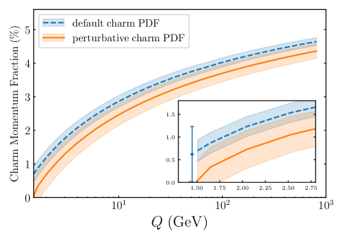
Figure E.1: The 4FNS charm momentum fraction in NNPDF4.0 as a function of scale $Q$, both for the default and perturbative charm cases, for a charm mass value of $m_{c}=1.51$ GeV. The inset zooms on the low-$Q$ region and includes the 3FNS (default) result from Table E.1. Note that the uncertainty includes the MHOU for the 3FNS default and 4FNS perturbative charm cases, while it is the PDF uncertainty for the 4FNS default charm case.

The 4FNS charm momentum fraction is plotted as a function of scale in Fig. E.1, both in the default case and for perturbative charm, with the 3FNS values and the detail of the low-$Q$ 4FNS results shown in an inset. The dependence on the value of the charm mass is shown in Fig. E.2. The large MHOUs on the 3FNS result, and on the 4FNS result in the case of perturbative charm, are apparent. The stability of the default result upon variation of the value of $m_{c}$, and the strong dependence of the perturbative charm result on $m_{c}$, are also clear. Both the large MHOU uncertainty, and the strong dependence on the value of $m_{c}$ for perturbative charm are seen to persist up to large scales.

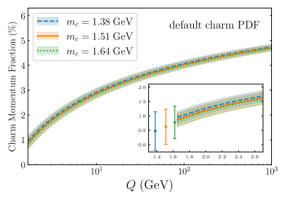
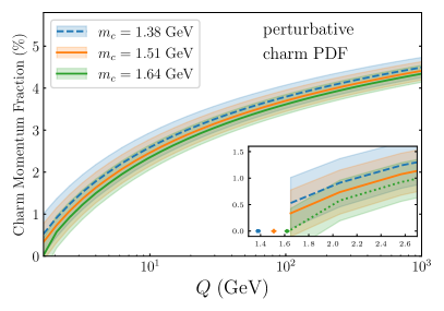
Figure E.2: Same as Fig. E.1 for different values of the charm mass. Note that the 3FNS momentum fraction for perturbative charm vanishes identically by assumption.

It is interesting to understand in detail the impact of the MHOU on the momentum fraction carried by intrinsic charm. To this purpose, we have computed the truncated momentum integral, i.e. Eq. (E.1) but only integrated down to some lower integration limit $x_{\rm min}$:

$$\left[c\right]_{\rm tr}(x_{\rm min})\equiv\int_{x_{\rm min}}^{1}dx\,xc^{+}(x,Q^{2})\,.$$ (E.2)

Note than in the 3FNS $xc^{+}(x)$ does not depend on scale, so this becomes a scale-independent quantity. The result for our default intrinsic charm determination is displayed in Fig. E.3, as a function of of the lower integration limit $x_{\rm min}$. It is clear that for $x_{\rm min}\gtrsim 0.2$ the truncated momentum fraction differs significantly from zero, thereby providing evidence for intrinsic charm with similar statistical significance as the local pull shown in Fig. 2 bottom left. For $x\mathrel{\hbox to0.0pt{\lower 4.0pt\hbox{\hskip 1.0pt$\sim$}\hss}\raise 1.0pt\hbox{$<$}}0.2$ this significance is then washed out by the large MHOUs.

Hence, while the total momentum fraction has been traditionally adopted as a measure of intrinsic charm, our analysis shows that, once MHOUs are accounted for, the information provided by the total momentum fraction is limited, at least with current data and theory.

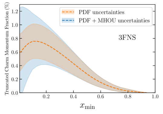
Figure E.3: The value of the truncated charm momentum integral, Eq. (E.2), as a function of the lower integration limit $x_{\rm min}$ for our baseline determination of the 3FNS intrinsic charm PDF. We display separately the PDF and the total (PDF+MHOU) uncertainties.

Appendix F Comparison with CT14IC

The possibility of an intrinsic charm component was recently studied in [18], by modifying the CT14 PDF set, with the initial 4FNS charm PDF taken equal to the BHPS model [1] form with the normalization fitted as a free parameter. A 4FNS charm PDF with uncertainties at $Q=1.3$ GeV was then constructed by taking the BHPS model with best-fit normalization as central value (called the ‘BHPS1 model’ in [18]); the lower edge of the uncertainty band was taken to coincide with the standard CT14 charm PDF (i.e. the charm PDF determined by perturbative matching from the 3FNS to the 4FNS); the upper edge of the uncertainty band was taken as the BHPS model but with normalization fixed to the upper 90% CL limit (called the ‘BHPS2 model’ in [18]).

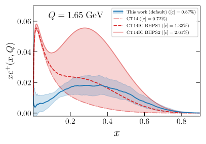
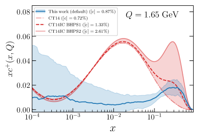
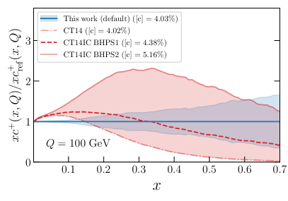
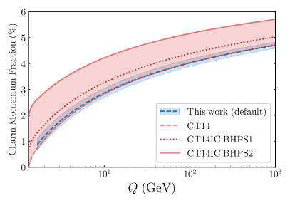
Figure F.1: The 4FNS charm PDF from [18] compared to our result (also in the 4FNS) at $Q=1.65$ GeV on a linear (top left) and logarithmic (top right) scale in $x$, and at $Q=100$ GeV on a linear scale in $x$ and as a ratio to our result (bottom left). The momentum fraction corresponding to either case is also shown as a function of $Q$ (bottom right). Note that for our result the uncertainty band is the 68%CL PDF uncertainty, while for [18] the central curve (labeled CT14IC BHPS1) corresponds to the BHPS model with best-fit normalization, the lower curve (labeled CT14) corresponds to the default CT14 perturbative charm PDF and the upper curve (labeled CT14IC BHPS2) corresponds to the BHPS model with normalization at the upper 90% CL (see text). The value of the momentum fractions are also provided in each case.

The CT14IC charm PDF is compared to our result in Fig. F.1, at $Q=1.65$ GeV and $Q=100$ GeV, in the former case on both a logarithmic and linear scale in $x$ and in the latter case on a linear scale only, as a ratio to our default result. Note that the uncertainty band has a different interpretation in the two curves shown: for our result it is the 68% CL PDF uncertainty, while for [18] it corresponds to the model uncertainty estimated as described above. In Fig. F.1 we also quote the charm momentum fraction in each case, at the corresponding scale $Q$.

As shown in Fig. 1 (right), our result for the charm PDF is in good agreement with the BHPS model at large $x$. Correspondingly, for $x\mathrel{\hbox to0.0pt{\lower 4.0pt\hbox{\hskip 1.0pt$\sim$}\hss}\raise 1.0pt\hbox{$>$}}0.3$ we find reasonably good agreement between our result and the central curve of [18], which corresponds to a momentum fraction and thus a normalization of the charm PDF not too different from our result (see Table E.1). Both the upper and lower curve from [18] instead do not agree with our result within uncertainties: indeed the lower edge corresponds to the absence of intrinsic charm (which we exclude) and the upper edge to a momentum fraction which we exclude at more than the $5\sigma$ level (see Table E.1).

For intermediate values $3\cdot 10^{-3}\mathrel{\hbox to0.0pt{\lower 4.0pt\hbox{\hskip 1.0pt$\sim$}\hss}\raise 1.0pt\hbox{$<$}}x\mathrel{\hbox to0.0pt{\lower 4.0pt\hbox{\hskip 1.0pt$\sim$}\hss}\raise 1.0pt\hbox{$<$}}0.3$ our result disagrees with that of  [18], while at very small $x$ all results agree, the intrinsic charm being compatible with zero. The disagreement at intermediate $x$ is mostly due to the fact that in  [18] charm is assumed to take the BHPS form, which vanishes for $x\mathrel{\hbox to0.0pt{\lower 4.0pt\hbox{\hskip 1.0pt$\sim$}\hss}\raise 1.0pt\hbox{$<$}}0.1$, in the 4FNS at the low scale $Q=1.3$ GeV. Due to perturbative evolution from $Q=1.3$ GeV to $Q=1.65$ GeV the charm PDF then develops the large bump that is seen in Fig. F.1, where we instead find that the 4FNS charm PDF is quite small. This difference persists at large scales as seen in Fig. 1 (bottom left).

In terms of momentum fractions, shown in Fig. 1 (bottom right), as already mentioned our result is compatible with the central value of [18] within uncertainties; and also with the lower edge of  [18] that corresponds to perturbative charm. The upper edge of the prediction from [18] is instead ruled out at more than $5\sigma$.

Appendix G $Z$+charm production in the forward region

Here we provide full details on our computation of $Z$+charm production and on the inclusion of the LHCb data for this process in the determination of the charm PDF shown in Fig. 2.

Computational settings.

Theoretical predictions for the $Z$+charm measurements in the forward region by LHCb [6] follow the settings described in [39]. $Z$+jet events at NLO QCD theory are generated for $\sqrt{s}=13$ TeV using the $Zj$ package of the POWHEG-BOX [40]. The parton-level events produced by POWHEG are then interfaced to Pythia8 [41] with the Monash 2013 tune Skands:2014pea for showering, hadronization, and simulation of the underlying event and multiple parton interactions. Long-lived hadrons, including charmed hadrons, are assumed stable and not decayed.

Selection criteria on these particle-level events are imposed to match the LHCb acceptance [6]. $Z$ bosons are reconstructed in the dimuon final state by requiring $60~{}{\rm GeV}\leq m_{\mu\mu}\leq 120~{}{\rm GeV}$, and only events where these muons satisfy $p_{T}^{\mu}\geq 20~{}{\rm GeV}$ and $2.0\leq\eta_{\mu}\leq 4.5$ are retained. Stable visible hadrons within the LHCb acceptance of $2.0\leq\eta\leq 4.5$ are clustered with the anti-$k_{T}$ algorithm with radius parameter of $R=0.5$ Cacciari:2008gp. Only events with a hardest jet satisfying $20~{}{\rm GeV}\leq p_{T}^{\rm jet}\leq 100~{}{\rm GeV}$ and $2.2\leq\eta_{\rm jet}\leq 4.2$ are retained. Charm jets are defined as jets containing a charmed hadron, specifically jets satisfying $\Delta R(j,c{\rm-hadron})\leq 0.5$ for a charmed hadron with $p_{T}(c{\rm-hadron})\geq 5~{}{\rm GeV}$. Jets and muons are required to be separated in rapidity and azimuthal angle, so we require $\Delta R(j,\mu)\geq 0.5$. The resulting events are then binned in the $Z$ bosom rapidity $y_{Z}=y_{\mu\mu}$.

The physical observable measured by LHCb is the ratio of the fraction of $Z$+jet events with and without a charm tag,

$$\mathcal{R}_{j}^{c}\equiv{{\sigma(pp\to Z+{\rm charm~{}jet})}\over{\sigma(pp\to Z+{\rm jet})}}={{N(c{\rm-tag})}\over{N({\rm jets})}}\,.$$ (G.1)

Here $N(c{\rm-tag})$ and $N({\rm jets})$ are, respectively, the number of charm-tagged and un-tagged jets, for a $Z$ boson rapidity interval that satisfies the selection and acceptance criteria. The denominator of Eq. (G.1) includes all jets, even those containing heavy hadrons. The charm tagging efficiency is already accounted for at the level of the experimental measurement, so it is not required in the theory simulations.

Predictions for Eq. (G.1) are produced using our default PDF determination (NNPDF4.0 NNLO), as well as the corresponding PDF set with perturbative charm (see SI Sect. B). We have explicitly checked that our results are essentially independent of the value of the charm mass. We have evaluated MHOUs and PDF uncertainties using the output of the POWHEG+Pythia8 calculations. We have checked that MHOUs, evaluated with the standard seven-point prescription, essentially cancel in the ratio Eq. (G.1). Note that this is not the case for PDF uncertainties, because the dominant partonic subchannels in the numerator and denominator are not the same.

Inclusion of the LHCb data.

$\chi^{2}/N_{\rm dat}$	default charm		perturbative charm
	$\rho_{\rm sys}=0$	$\rho_{\rm sys}=1$	$\rho_{\rm sys}=0$	$\rho_{\rm sys}=1$
Prior	1.85	3.33	3.54	3.85
Reweighted	1.81	3.14	$-$	$-$

Table G.1: The values of $\chi^{2}/N_{\rm dat}$ for the LHCb $Z$+charm data before (prior) and after (reweighted) their inclusion in the PDF fit. Results are given for two experimental correlation models, denoted as $\rho_{\rm sys}=0$ and $\rho_{\rm sys}=1$. We also report values before inclusion for the perturbative charm PDFs.

We first compare the quality of the description of the LHCb data before their inclusion. In Table G.1 we show the values of $\chi^{2}/N_{\rm dat}$ for the LHCb $Z$+charm data both with default and perturbative charm. Since the experimental covariance matrix is not available for the LHCb data we determine the $\chi^{2}$ values assuming two limiting scenarios for the correlation of experimental systematic uncertainties. Namely, we either add in quadrature statistical and systematic errors ($\rho_{\rm sys}=0$), or alternatively we assume that the total systematic uncertainty is fully correlated between $y_{Z}$ bins ($\rho_{\rm sys}=1$). Fit quality is always significantly better in our default intrinsic charm scenario than with perturbative charm. As is clear from Fig. 2 (top left), the somewhat poor fit quality is mostly due to the first rapidity bin, which is essentially uncorrelated to the amount of intrinsic charm (see Fig. 2, top right).

The LHCb $Z$+charm data are then included in the PDF determination through Bayesian reweighting Ball:2010gb,Ball:2011gg. The $\chi^{2}/N_{\rm dat}$ values obtained using the PDFs found after their inclusion are given in Table G.1. They are computed by combining the PDF and experimental covariance matrix so both sources of uncertainty are included — as mentioned above, MHOUs are negligible. The fit quality is seen to improve only mildly, and the effective number of replicas Ball:2010gb,Ball:2011gg after reweighting is only moderately reduced, from the prior $N_{\rm rep}=100$ to $N_{\rm eff}=92$ or $N_{\rm eff}=84$ in the $\rho_{\rm sys}=0$ and $\rho_{\rm sys}=1$ scenarios respectively. This demonstrates that the inclusion of the LHCb $Z$+charm measurements affects the PDFs only weakly. This agrees with the results shown in Figs. 2 (center) in the main manuscript, where it is seen that the inclusion of the LHCb data has essentially no impact on the shape of the charm PDF, but it moderately reduces its uncertainty in the region of the valence peak.

Appendix H Parton luminosities

The impact of intrinsic charm on hadron collider observables can be assessed by studying parton luminosities. Indeed, the cross-section for hadronic processes at leading order is typically proportional to an individual parton luminosity or linear combination of parton luminosities. Comparing parton luminosities determined using our default PDF set to those obtained imposing perturbative charm (see SI Sect. B) provides a qualitative estimate of the measurable impact of intrinsic charm. Of course this is then modified by higher-order perturbative corrections, which generally depend on more partonic subchannels and thus on more luminosities. In this section we illustrate this by considering the parton luminosities that are relevant for the computation of the $Z$+charm process in the LHCb kinematics, see SI Sect. G.

The parton luminosity without any restriction on the rapidity $y_{X}$ of the final state is

$$\mathcal{L}_{ab}(m_{X})={{1}\over{s}}\int_{\tau}^{1}{{dx}\over{x}}f_{a}\left(x,m_{X}^{2}\right)f_{b}\left(\tau/x,m_{X}^{2}\right)\,,\qquad\tau={{m_{X}^{2}}\over{s}}\,,$$ (H.1)

where $a,b$ label the species of incoming partons, $\sqrt{s}$ is the center-of-mass energy of the hadronic collision, and $m_{X}$ is the final state invariant mass. For the more realistic situation where the final state rapidity is restricted, $y_{\rm min}\leq y_{X}\leq y_{\rm max}$, Eq. (H.1) is modified as

$$\mathcal{L}_{ab}(m_{X})={{1}\over{s}}\int_{\tau}^{1}{{dx}\over{x}}f_{a}\left(x,m_{X}^{2}\right)f_{b}\left(\tau/x,m_{X}^{2}\right)\theta\left(y_{X}-y_{\rm min}\right)\theta\left(y_{\rm max}-y_{X}\right)\,,$$ (H.2)

where $y_{X}=\left(\ln x^{2}/\tau\right)/2$.

We consider in particular the quark-gluon and the charm-gluon luminosities, defined as

$$\mathcal{L}_{qg}(m_{X})\equiv\sum_{i=1}^{n_{f}}\left(\mathcal{L}_{q_{i}g}(m_{X})+\mathcal{L}_{\bar{q}_{i}g}(m_{X})\right)\,,\quad\mathcal{L}_{cg}(m_{X})\equiv\left(\mathcal{L}_{cg}(m_{X})+\mathcal{L}_{\bar{c}g}(m_{X})\right)\,,$$ (H.3)

where $n_{f}$ is the number of active quark flavors for a given value of $Q=m_{X}$ with a maximum value of $n_{f}=5$. These are the combinations that provide the leading contributions respectively to the numerator ($\mathcal{L}_{cg}$) and the denominator ($\mathcal{L}_{qg}$) of $\mathcal{R}_{j}^{c}$ in Eq. (G.1).

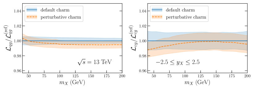
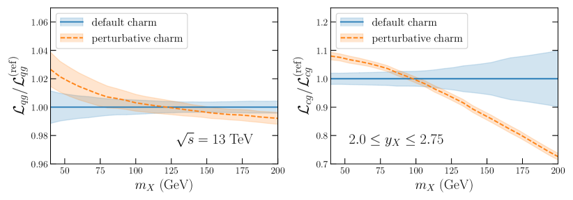
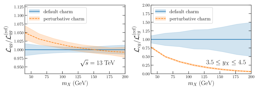
Figure H.1: The quark-gluon (left) and charm-gluon (right) parton luminosities in the $m_{X}$ region relevant for $Z$+charm production and three different rapidity bins (see text). Results are shown both for our default charm PDFs and for the variant with perturbative charm.

The luminosities are displayed in Fig. H.1, in the invariant mass region, $40~{}{\rm GeV}\leq m_{X}\leq 200~{}{\rm GeV}$ which is most relevant for $Z$+charm production. Results are shown for three different rapidity bins, $-2.5\leq y_{X}\leq 2.5$ (central production in ATLAS and CMS), $2.0\leq y_{X}\leq 2.75$ (forward production, corresponding to the central bin in LHCb), and $3.5\leq y_{X}\leq 4.5$ (highly boosted production, corresponding to the most forward bin in the LHCb selection), as a ratio to our default case.

For central production it is clear that both the quark-gluon and charm-gluon luminosities with our without intrinsic charm are very similar. This means that central $Z$+charm production in this invariant mass range is insensitive to intrinsic charm. For forward production, corresponding to the central LHCb rapidity bin, $2.0\leq y_{X}\leq 2.75$, in the invariant mass region $m_{X}\simeq 100$ GeV again there is little difference between results with or without intrinsic charm, but as the invariant mass increases the charm-gluon luminosity with intrinsic charm is significantly enhanced. For very forward production, such as the highest rapidity bin of LHCb, $3.5\leq y_{X}\leq 4.5$, the charm-gluon luminosity at $m_{X}\simeq 100$ GeV is enhanced by a factor of about 4 in our default result in comparison to the perturbative charm case, corresponding to a $\simeq 3\sigma$ difference in units of the PDF uncertainty, consistently with the behavior observed for the $\mathcal{R}_{j}^{c}$ observable in Fig. 2 (top left) in the most forward rapidity bin. This observation provides a qualitative explanation of the results of SI Sect. G.

References

- [1] S. J. Brodsky, P. Hoyer, C. Peterson, and N. Sakai, The Intrinsic Charm of the Proton, Phys. Lett. B93 (1980) 451–455.
- [2] S. J. Brodsky, A. Kusina, F. Lyonnet, I. Schienbein, H. Spiesberger, and R. Vogt, A review of the intrinsic heavy quark content of the nucleon, Adv. High Energy Phys. 2015 (2015) 231547, [arXiv:1504.06287].
- [3] NNPDF Collaboration, R. D. Ball et al., The path to proton structure at 1% accuracy, Eur. Phys. J. C 82 (2022), no. 5 428, [arXiv:2109.02653].
- [4] R. D. Ball, V. Bertone, M. Bonvini, S. Forte, P. Groth Merrild, J. Rojo, and L. Rottoli, Intrinsic charm in a matched general-mass scheme, Phys. Lett. B754 (2016) 49–58, [arXiv:1510.00009].
- [5] T. J. Hobbs, J. T. Londergan, and W. Melnitchouk, Phenomenology of nonperturbative charm in the nucleon, Phys. Rev. D 89 (2014), no. 7 074008, [arXiv:1311.1578].
- [6] LHCb Collaboration, R. Aaij et al., Study of Z Bosons Produced in Association with Charm in the Forward Region, Phys. Rev. Lett. 128 (2022), no. 8 082001, [arXiv:2109.08084].
- [7] R. P. Feynman, The behavior of hadron collisions at extreme energies, Conf. Proc. C 690905 (1969) 237–258.
- [8] J. Gao, L. Harland-Lang, and J. Rojo, The Structure of the Proton in the LHC Precision Era, Phys. Rept. 742 (2018) 1–121, [arXiv:1709.04922].
- [9] R. Abdul Khalek et al., Science Requirements and Detector Concepts for the Electron-Ion Collider: EIC Yellow Report, arXiv:2103.05419.
- [10] J. L. Feng et al., The Forward Physics Facility at the High-Luminosity LHC, arXiv:2203.05090.
- [11] IceCube-Gen2 Collaboration, M. G. Aartsen et al., IceCube-Gen2: the window to the extreme Universe, J. Phys. G 48 (2021), no. 6 060501, [arXiv:2008.04323].
- [12] M. Constantinou et al., Parton distributions and lattice-QCD calculations: Toward 3D structure, Prog. Part. Nucl. Phys. 121 (2021) 103908, [arXiv:2006.08636].
- [13] A. De Roeck and R. S. Thorne, Structure Functions, Prog.Part.Nucl.Phys. 66 (2011) 727, [arXiv:1103.0555].
- [14] K. Kovařík, P. M. Nadolsky, and D. E. Soper, Hadronic structure in high-energy collisions, Rev. Mod. Phys. 92 (2020), no. 4 045003, [arXiv:1905.06957].
- [15] J. Rojo, The Partonic Content of Nucleons and Nuclei, arXiv:1910.03408.
- [16] S. J. Brodsky, J. C. Collins, S. D. Ellis, J. F. Gunion, and A. H. Mueller, Intrinsic Chevrolets at the SSC, in 1984 DPF Summer Study on the Design and Utilization of the Superconducting Super Collider (SSC) (Snowmass 84), p. 227, 8, 1984.
- [17] P. Jimenez-Delgado, T. Hobbs, J. Londergan, and W. Melnitchouk, New limits on intrinsic charm in the nucleon from global analysis of parton distributions, Phys.Rev.Lett. 114 (2015), no. 8 082002, [arXiv:1408.1708].
- [18] T.-J. Hou, S. Dulat, J. Gao, M. Guzzi, J. Huston, P. Nadolsky, C. Schmidt, J. Winter, K. Xie, and C. P. Yuan, CT14 Intrinsic Charm Parton Distribution Functions from CTEQ-TEA Global Analysis, JHEP 02 (2018) 059, [arXiv:1707.00657].
- [19] G. Heinrich, Collider Physics at the Precision Frontier, Phys. Rept. 922 (2021) 1–69, [arXiv:2009.00516].
- [20] S. Forte, E. Laenen, P. Nason, and J. Rojo, Heavy quarks in deep-inelastic scattering, Nucl. Phys. B834 (2010) 116–162, [arXiv:1001.2312].
- [21] R. D. Ball, M. Bonvini, and L. Rottoli, Charm in Deep-Inelastic Scattering, JHEP 11 (2015) 122, [arXiv:1510.02491].
- [22] NNPDF Collaboration, R. D. Ball, V. Bertone, M. Bonvini, S. Carrazza, S. Forte, A. Guffanti, N. P. Hartland, J. Rojo, and L. Rottoli, A Determination of the Charm Content of the Proton, Eur. Phys. J. C76 (2016), no. 11 647, [arXiv:1605.06515].
- [23] NNPDF Collaboration, R. D. Ball et al., Parton distributions from high-precision collider data, Eur. Phys. J. C77 (2017), no. 10 663, [arXiv:1706.00428].
- [24] J. C. Collins and W.-K. Tung, Calculating Heavy Quark Distributions, Nucl. Phys. B 278 (1986) 934.
- [25] M. Buza, Y. Matiounine, J. Smith, and W. L. van Neerven, Charm electroproduction viewed in the variable-flavour number scheme versus fixed-order perturbation theory, Eur. Phys. J. C1 (1998) 301–320, [hep-ph/9612398].
- [26] I. Bierenbaum, J. Blümlein, and S. Klein, The Gluonic Operator Matrix Elements at for DIS Heavy Flavor Production, Phys. Lett. B 672 (2009) 401–406, [arXiv:0901.0669].
- [27] I. Bierenbaum, J. Blümlein, and S. Klein, Mellin Moments of the Heavy Flavor Contributions to unpolarized Deep-Inelastic Scattering at and Anomalous Dimensions, Nucl. Phys. B 820 (2009) 417–482, [arXiv:0904.3563].
- [28] J. Ablinger, J. Blümlein, S. Klein, C. Schneider, and F. Wissbrock, The Massive Operator Matrix Elements of for the Structure Function and Transversity, Nucl. Phys. B 844 (2011) 26–54, [arXiv:1008.3347].
- [29] J. Ablinger, A. Behring, J. Blümlein, A. De Freitas, A. Hasselhuhn, A. von Manteuffel, M. Round, C. Schneider, and F. Wißbrock, The 3-Loop Non-Singlet Heavy Flavor Contributions and Anomalous Dimensions for the Structure Function and Transversity, Nucl. Phys. B 886 (2014) 733–823, [arXiv:1406.4654].
- [30] J. Ablinger, J. Blümlein, A. De Freitas, A. Hasselhuhn, A. von Manteuffel, M. Round, and C. Schneider, The Contributions to the Gluonic Operator Matrix Element, Nucl. Phys. B 885 (2014) 280–317, [arXiv:1405.4259].
- [31] A. Behring, I. Bierenbaum, J. Blümlein, A. De Freitas, S. Klein, and F. Wißbrock, The logarithmic contributions to the asymptotic massive Wilson coefficients and operator matrix elements in deeply inelastic scattering, Eur. Phys. J. C 74 (2014), no. 9 3033, [arXiv:1403.6356].
- [32] J. Ablinger, J. Blümlein, A. De Freitas, A. Hasselhuhn, A. von Manteuffel, M. Round, C. Schneider, and F. Wißbrock, The transition matrix element of the variable flavor number scheme at , Nuclear Physics B 882 (May, 2014) 263–288.
- [33] J. Ablinger, A. Behring, J. Blümlein, A. De Freitas, A. von Manteuffel, et al., The 3-Loop Pure Singlet Heavy Flavor Contributions to the Structure Function and the Anomalous Dimension, arXiv:1409.1135.
- [34] J. Blümlein, J. Ablinger, A. Behring, A. De Freitas, A. von Manteuffel, C. Schneider, and C. Schneider, Heavy Flavor Wilson Coefficients in Deep-Inelastic Scattering: Recent Results, PoS QCDEV2017 (2017) 031, [arXiv:1711.07957].
- [35] E. Hoffmann and R. Moore, Subleading Contributions to the Intrinsic Charm of the Nucleon, Z. Phys. C 20 (1983) 71.
- [36] J. Pumplin, Light-cone models for intrinsic charm and bottom, Phys. Rev. D 73 (2006) 114015, [hep-ph/0508184].
- [37] S. Paiva, M. Nielsen, F. S. Navarra, F. O. Duraes, and L. L. Barz, Virtual meson cloud of the nucleon and intrinsic strangeness and charm, Mod. Phys. Lett. A 13 (1998) 2715–2724, [hep-ph/9610310].
- [38] F. M. Steffens, W. Melnitchouk, and A. W. Thomas, Charm in the nucleon, Eur. Phys. J. C 11 (1999) 673–683, [hep-ph/9903441].
- [39] T. Boettcher, P. Ilten, and M. Williams, Direct probe of the intrinsic charm content of the proton, Phys. Rev. D 93 (2016), no. 7 074008, [arXiv:1512.06666].
- [40] S. Alioli, P. Nason, C. Oleari, and E. Re, A general framework for implementing NLO calculations in shower Monte Carlo programs: the POWHEG BOX, JHEP 1006 (2010) 043, [arXiv:1002.2581].
- [41] T. Sjostrand, S. Mrenna, and P. Z. Skands, A Brief Introduction to PYTHIA 8.1, Comput. Phys. Commun. 178 (2008) 852–867, [arXiv:0710.3820].
- [42] European Muon Collaboration, J. J. Aubert et al., Production of charmed particles in 250-GeV - iron interactions, Nucl. Phys. B213 (1983) 31–64.
- [43] B. W. Harris, J. Smith, and R. Vogt, Reanalysis of the EMC charm production data with extrinsic and intrinsic charm at NLO, Nucl. Phys. B 461 (1996) 181–196, [hep-ph/9508403].
- [44] HL-LHC, HE-LHC Working Group Collaboration, P. Azzi et al., Standard Model Physics at the HL-LHC and HE-LHC, arXiv:1902.04070.
- [45] LHCb Collaboration, R. Aaij et al., First Measurement of Charm Production in its Fixed-Target Configuration at the LHC, Phys. Rev. Lett. 122 (2019), no. 13 132002, [arXiv:1810.07907].
- [46] QCD Working Group Collaboration, A. Dainese et al., Physics Beyond Colliders: QCD Working Group Report, arXiv:1901.04482.
- [47] C. Hadjidakis et al., A fixed-target programme at the LHC: Physics case and projected performances for heavy-ion, hadron, spin and astroparticle studies, Phys. Rept. 911 (2021) 1–83, [arXiv:1807.00603].
- [48] L. A. Anchordoqui et al., The Forward Physics Facility: Sites, experiments, and physics potential, Phys. Rept. 968 (2022) 1–50, [arXiv:2109.10905].
- [49] F. Halzen and L. Wille, Charm contribution to the atmospheric neutrino flux, Phys. Rev. D 94 (2016), no. 1 014014, [arXiv:1605.01409].
- [50] NNPDF Collaboration, R. D. Ball et al., Parton distributions from high-precision collider data, Eur. Phys. J. C 77 (2017), no. 10 663, [arXiv:1706.00428].
- [51] NNPDF Collaboration, R. D. Ball et al., An open-source machine learning framework for global analyses of parton distributions, Eur. Phys. J. C 81 (2021), no. 10 958, [arXiv:2109.02671].
- [52] V. Bertone, S. Carrazza, and J. Rojo, APFEL: A PDF Evolution Library with QED corrections, Comput.Phys.Commun. 185 (2014) 1647, [arXiv:1310.1394].
- [53] A. Candido, F. Hekhorn, and G. Magni, EKO: Evolution Kernel Operators, arXiv:2202.02338.
- [54] G. P. Salam and J. Rojo, A Higher Order Perturbative Parton Evolution Toolkit (HOPPET), Comput. Phys. Commun. 180 (2009) 120–156, [arXiv:0804.3755].
- [55] M. Botje, QCDNUM: Fast QCD Evolution and Convolution, Comput.Phys.Commun. 182 (2011) 490–532, [arXiv:1005.1481].
- [56] A. Vogt, Efficient evolution of unpolarized and polarized parton distributions with qcd-pegasus, Comput. Phys. Commun. 170 (2005) 65–92, [hep-ph/0408244].
- [57] The NNPDF Collaboration, L. Del Debbio, S. Forte, J. I. Latorre, A. Piccione, and J. Rojo, Neural network determination of parton distributions: The nonsinglet case, JHEP 03 (2007) 039, [hep-ph/0701127].
- [58] The NNPDF Collaboration, R. D. Ball et al., A determination of parton distributions with faithful uncertainty estimation, Nucl. Phys. B809 (2009) 1–63, [arXiv:0808.1231].
- [59] The NNPDF Collaboration, R. D. Ball et al., A first unbiased global NLO determination of parton distributions and their uncertainties, Nucl. Phys. B838 (2010) 136, [arXiv:1002.4407].
- [60] S. Zanoli, Higher-order matching for heavy quarks in perturbative QCD, . MSc Thesis, University of Milano, 2020.
- [61] M. Dittmar et al., Working Group I: Parton distributions: Summary report for the HERA LHC Workshop Proceedings, hep-ph/0511119.
- [62] W. Giele et al., The QCD / SM working group: Summary report, in 2nd Les Houches Workshop on Physics at TeV Colliders, pp. 275–426, 4, 2002. hep-ph/0204316.
- [63] LHC Higgs Cross Section Working Group Collaboration, D. de Florian et al., Handbook of LHC Higgs Cross Sections: 4. Deciphering the Nature of the Higgs Sector, arXiv:1610.07922.
- [64] C. W. Bauer, Z. Ligeti, M. Luke, A. V. Manohar, and M. Trott, Global analysis of inclusive B decays, Phys. Rev. D 70 (2004) 094017, [hep-ph/0408002].
- [65] P. Skands, S. Carrazza, and J. Rojo, Tuning PYTHIA 8.1: the Monash 2013 Tune, European Physical Journal 74 (2014) 3024, [arXiv:1404.5630].
- [66] M. Cacciari, G. P. Salam, and G. Soyez, The Anti-k(t) jet clustering algorithm, JHEP 0804 (2008) 063, [arXiv:0802.1189].
- [67] The NNPDF Collaboration, R. D. Ball et al., Reweighting NNPDFs: the W lepton asymmetry, Nucl. Phys. B849 (2011) 112–143, [arXiv:1012.0836].
- [68] R. D. Ball, V. Bertone, F. Cerutti, L. Del Debbio, S. Forte, et al., Reweighting and Unweighting of Parton Distributions and the LHC W lepton asymmetry data, Nucl.Phys. B855 (2012) 608–638, [arXiv:1108.1758].