Position-aware Structure Learning for Graph Topology-imbalance by Relieving Under-reaching and Over-squashing

Abstract.

Topology-imbalance is a graph-specific imbalance problem caused by the uneven topology positions of labeled nodes, which significantly damages the performance of GNNs. What topology-imbalance means and how to measure its impact on graph learning remain under-explored. In this paper, we provide a new understanding of topology-imbalance from a global view of the supervision information distribution in terms of under-reaching and over-squashing, which motivates two quantitative metrics as measurements. In light of our analysis, we propose a novel position-aware graph structure learning framework named PASTEL, which directly optimizes the information propagation path and solves the topology-imbalance issue in essence. Our key insight is to enhance the connectivity of nodes within the same class for more supervision information, thereby relieving the under-reaching and over-squashing phenomena. Specifically, we design an anchor-based position encoding mechanism, which better incorporates relative topology position and enhances the intra-class inductive bias by maximizing the label influence. We further propose a class-wise conflict measure as the edge weights, which benefits the separation of different node classes. Extensive experiments demonstrate the superior potential and adaptability of PASTEL in enhancing GNNs’ power in different data annotation scenarios.

1. Introduction

Graph learning (Zhang et al., 2020; Li et al., 2022; Fu et al., 2021) has gained popularity over the past years due to its versatility and success in representing graph data across a wide range of domains (Nastase et al., 2015; Sun et al., 2020; Gao et al., 2021; Yu et al., 2022; Chen et al., 2022). Graph Neural Networks (GNNs) (Wu et al., 2020; Sun et al., 2021) have been the “battle horse” of graph learning, which propagate the features on the graph by exchanging information between neighbors in a message-passing paradigm (Gilmer et al., 2017). Due to the asymmetric and uneven topology, learning on graphs by GNNs suffers a specific imbalance problem, i.e., topology-imbalance. Topology-imbalance (Chen et al., 2021) is caused by the uneven position distribution of labeled nodes in the topology space, which is inevitable in real-world applications due to data availability and the labeling costs. For example, we may only have information for a small group of users within a local community in social networks, resulting in a serious imbalance of labeled node positions. The uneven position distribution of labeled nodes leads to uneven information propagation, resulting in the poor quality of learned representations.

Although the imbalance learning on graphs has attracted many research interests in recent years, most of them focus on the class-imbalance issue (Park et al., 2021; Wang et al., 2021), i.e., the imbalanced number of labeled nodes of each class. The topology-imbalance issue is proposed recently and is still under-explored. The only existing work, ReNode (Chen et al., 2021), provides an understanding of the topology-imbalance issue from the perspective of label propagation and proposes a sample re-weighting method. However, ReNode takes the node topological boundaries as decision boundaries based on a homophily assumption, which does not work with real-world graphs. The strong assumption leads to poor generalization and unsatisfied performance of ReNode (see Section 5.2.1). There are two remaining questions: (1) Why does topology-imbalance affect the performance of graph representation learning? and (2) What kind of graphs are susceptible to topology-imbalance? To answer the above two questions, how to measure the influence of labeled nodes is the key challenge in handling topology-imbalance due to the complex graph connections and the unknown class labels for most nodes in the graph.

Figure 1. Schematic diagram of under-reaching and over-squashing in the topology-imbalance issue.

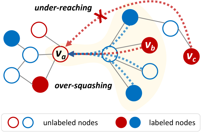
New understanding for topology-imbalance. In this work, we provide a new understanding of the topology-imbalance issue from a global view of the supervision information distribution in terms of under-reaching and over-squashing: (1) Under-reaching: the influence of labeled nodes decays with the topology distance (Buchnik and Cohen, 2018), resulting in the nodes far away from labeled nodes lack of supervision information. In Figure 1, the node $v_{a}$ cannot reach the valuable labeled node $v_{c}$ within the receptive field of the GNN model, resulting in the quantity of information it received is limited. (2) Over-squashing: the supervision information of valuable labeled nodes is squashed when passing across the narrow path together with other useless information. In Figure 1, the valuable supervision information of $v_{b}$ to $v_{a}$ is compressed into a vector together with the information of many nodes belonging to other classes, resulting in the quality of supervision information that $v_{a}$ received being poor. Then we introduce two metrics (reaching coefficient and squashing coefficient) to give a quantitative analysis of the relation between the learning performance, label positions, and graph structure properties. We further draw a conclusion that better reachability and lower squashing to labeled nodes lead to better classification performance for GNN models.

Present work. In light of the above analysis, we propose a Position-Aware STructurE Learning method named PASTEL, which directly optimizes the information propagation path and solves the problem of topology-imbalance issue in essence. The key insight of PASTEL is to enable nodes within the same class to connect more closely with each other for more supervision information. Specifically, we design a novel anchor-based position encoding mechanism to capture the relative position between nodes and incorporate the position information into structure learning. Then we design a class-wise conflict measure based on the Group PageRank, which measures the influence from labeled nodes of each class and acts as a guide to increase the intra-class connectivity via adjusting edge weight. The main contributions are as follows:

• We provide a new understanding of the topology-imbalance issue from the perspective of supervision information distribution in terms of under-reaching and over-squashing and provide two new quantitative metrics for them.

• Equipped with the proposed position encodings and class-wise conflict measure, PASTEL can better model the relationships of node pairs and enhance the intra-class inductive bias by maximizing the label influence.

• Experimental results demonstrate that the proposed PASTEL enjoys superior effectiveness and indeed enhances the GNN model’s power for in-the-wild extrapolation.

2. Related Work

2.1. Imbalance Learning

Imbalanced classification problems (Sun et al., 2009; He and Garcia, 2009) have attracted extensive research attention. Most existing works (Haixiang et al., 2017; Lin et al., 2017) focus on the class-imbalance problem, where the model performance is dominated by the majority class. The class-imbalance learning methods can be roughly divided into two types: data-level re-sampling and algorithm-level re-weighting. Re-sampling methods re-sample (Chawla et al., 2002; Ando and Huang, 2017; Xiaolong et al., 2019) or augment data (Park et al., 2021) to balance the number of data for each class during the data selection phase. Re-weighting methods (Cao et al., 2019; Cui et al., 2019; Ren et al., 2018) adjust different weights to different data samples according to the number of data during the training phase.

For the graph-specific topology-imbalance issue as mentioned in Section 1, directly applying these methods to the graph data fails to take the special topology properties into consideration. ReNode (Chen et al., 2021) is the first work for the graph topology-imbalance issue, which follows the paradigm of classical re-weighting methods. Specifically, ReNode defines an influence conflict detection based metric and re-weights the labeled nodes based on their relative positions to class boundaries. However, ReNode is limited by its homophily assumption and only has a slight performance improvement. In this paper, PASTEL alleviates topology-imbalance by learning a new structure that maximizes the intra-class label influence, which can be seen as “label re-distribution” in the topology space.

2.2. Graph Structure Learning

Graph structure learning (Zhu et al., 2022) learns an optimized graph structure for representation learning and most of them aim to improve the robustness (Jin et al., 2020; Zheng et al., 2020) of GNN models. There are also some works (Franceschi et al., 2019; Chen et al., 2020b; Topping et al., 2022; Chen et al., 2020c; Sun et al., 2022) that utilize the structure learning to improve the graph representation quality. As for the over-squashing problem, (Wang and Leskovec, 2021) assigns different weights to edges connected to two nodes of the same class for better representations. However, (Wang and Leskovec, 2021) still fails with the issue of under-reaching. SDRF (Topping et al., 2022) rewires edges according to the Ricci curvatures to solve the over-squashing problem by only considering topology properties.

Multiple measurements in existing structure learning works are leveraged for modeling node relations, including node features (Zhao et al., 2021), node degrees (Jin et al., 2020), node encodings (Zhang et al., 2019) and edge attributes (Zheng et al., 2020). The node positions play an important role in generating discriminative representations (You et al., 2019) and are seldom considered in structure learning. In this work, we advance the structure learning strategy for the graph topology-imbalance issue and introduce a position-aware framework to better capture the nodes’ underlying relations.

3. Understanding Topology-Imbalance

In this section, we provide a new understanding of the topology-imbalance issue in terms of under-reaching and over-squashing. Then we perform a quantitative analysis of the relations between them to answer two questions:

Q1: Why does topology-imbalance affect the performance of graph representation learning?

Q2: What kind of graphs are susceptible to topology-imbalance?

3.1. Notations and Preliminaries

Consider a graph $\mathcal{G}=\{\mathcal{V},\mathcal{E}\}$, where $\mathcal{V}$ is the set of $N$ nodes and $\mathcal{E}$ is the edge set. Let $\mathbf{A}\in\mathbb{R}^{N\times N}$ be the adjacency matrix and $\mathbf{X}\in\mathbb{R}^{N\times d_{0}}$ be the node attribute matrix, where $d_{0}$ denotes the dimension of node attributes. The diagonal degree matrix is denoted as $\mathbf{D}\in\mathbb{R}^{N\times N}$ where $\mathbf{D}_{ii}=\sum^{N}_{j=1}\mathbf{A}_{ij}$. The graph diameter is denoted as $D_{\mathcal{G}}$. Given the labeled node set $\mathcal{V}_{L}$and their labels $\mathcal{Y}_{L}$ where each node $v_{i}$ is associated with a label $y_{i}$, semi-supervised node classification aims to train a node classifier $f_{\theta}:v\rightarrow\mathbb{R}^{C}$ to predict the labels $\mathcal{Y}_{U}$ of remaining nodes $\mathcal{V}_{U}=\mathcal{V}\setminus\mathcal{V}_{L}$, where $C$ denotes the number of classes. we separate the labeled node set $\mathcal{V}_{L}$ into $\{\mathcal{V}^{1}_{L},\mathcal{V}^{2}_{L},\cdots,\mathcal{V}^{C}_{L}\}$, where $\mathcal{V}^{i}_{L}$ is the nodes of class $i$ in $\mathcal{V}_{L}$.

3.2. Understanding Topology-Imbalance via Under-reaching and Over-squashing

In GNNs, node representations are learned by aggregating information from valuable neighbors. The quantity and quality of the information received by the nodes decide the expressiveness of their representations. We perceive the imbalance of the labeled node positions affects the performance of GNNs for two reasons:

(1) Under-reaching: The influence from labeled nodes decays with the topology distance (Buchnik and Cohen, 2018), resulting in that the nodes far away from labeled nodes lack supervision information. When the node can’t reach enough valuable labeled nodes within the receptive field of the model, the quantity of information it received is limited.

(2) Over-squashing: The receptive field of GNNs is exponentially-growing and all information is compressed into fixed-length vectors (Alon and Yahav, 2021). The supervision information of valuable labeled nodes is squashed when passing across the narrow path together with other useless information.

3.3. Quantitative Analysis

To provide quantitative analysis for topology-imbalance, we propose two metrics for reachability and squashing. First, we define a reaching coefficient based on the shortest path, which determines the minimum layers of GNNs to obtain supervision information:

Definition 1 (Reaching coefficient).

Given a graph $\mathcal{G}$ and labeled node set $\mathcal{V}_{L}$, the reaching coefficient $RC$ of $\mathcal{G}$ is the mean length of the shortest path from unlabeled nodes to the labeled nodes of their corresponding classes:

(1) $$RC=\frac{1}{|\mathcal{V}_{U}|}\sum_{v_{i}\in\mathcal{V}_{U}}\frac{1}{|\mathcal{V}^{y_{i}}_{L}|}\sum_{v_{j}\in\mathcal{V}^{y_{i}}_{L}}\left(1-\frac{\log|\mathcal{P}_{sp}(v_{i},v_{j})|}{\log D_{\mathcal{G}}}\right),$$

where $\mathcal{V}^{y_{i}}_{L}$ denotes the nodes in $\mathcal{V}_{L}$ whose label is $y_{i}$, $\mathcal{P}_{sp}(v_{i},v_{j})$ denotes the shortest path between $v_{i}$ and $v_{j}$, and $|\mathcal{P}_{sp}(v_{i},v_{j})|$ denotes its length, and $D_{\mathcal{G}}$ is the diameter of graph $\mathcal{G}$. Specifically, for the unconnected $v_{i}$ and $v_{j}$, we set the length of their shortest path as $D_{\mathcal{G}}$.

The reaching coefficient reflects how long the the distance when the GNNs passes the valuable information to the unlabeled nodes. Note that $RC\in[0,1)$ and larger $RC$ means better reachability.

For the quantitative metric of over-squashing, we define a squashing coefficient using the Ricci curvature to formulate it from a geometric perspective. The Ricci curvature (Ollivier, 2009) reflects the change of topology properties of the two endpoints of an edge, where the negative $Ric(v_{i},v_{j})$ means that the edge behaves locally as a shortcut or bridge and positive $Ric(v_{i},v_{j})$ indicates that locally there are more triangles in the neighborhood of $v_{i}$ and $v_{j}$ (Ni et al., 2015; Topping et al., 2022).

Definition 2 (Squashing coefficient).

Given a graph $\mathcal{G}$, the squashing coefficient $SC$ of $\mathcal{G}$ is the mean Ricci curvature of edges on the shortest path from unlabeled nodes to the labeled nodes of their corresponding classes:

(2) $$SC=\frac{1}{|\mathcal{V}_{U}|}\sum_{v_{i}\in\mathcal{V}_{U}}\frac{1}{|\mathcal{N}_{y_{i}}(v_{i})|}\sum_{v_{j}\in\mathcal{N}_{y_{i}}(v_{i})}\frac{\sum_{e_{kt}\in\mathcal{P}_{sp}(v_{i},v_{j})}Ric(v_{k},v_{t})}{|\mathcal{P}_{sp}(v_{i},v_{j})|},$$

where $\mathcal{N}_{y_{i}}(v_{i})$ denotes the labeled nodes of class $y_{i}$ that can reach $v_{i}$, $Ric(\cdot,\cdot)$ denotes the Ricci curvature, and $|\mathcal{P}_{sp}(v_{i},v_{j})|$ denotes the length of shortest path between $v_{i}$ and $v_{j}$.

We leverage the Ollivier-Ricci curvature (Ollivier, 2009) as $Ric(\cdot,\cdot)$ here:

(3) $$Ric(v_{k},v_{t})=\frac{Wasserstein(mass_{k},mass_{t})}{d_{geo}(v_{k},v_{t})},$$

where $Wasserstein(\cdot,\cdot)$ is the Wasserstein distance, $d_{geo}(\cdot,\cdot)$ is the geodesic distance function, and $mass_{k}$ is the mass distribution (Ollivier, 2009) of node $v_{k}$. Note that $SC$ can be either positive or negative and larger $SC$ means lower squashing because the ring structures are more friendly for information sharing.

Figure 2. Predictions of GCN with the same graph structure and different labeled nodes.

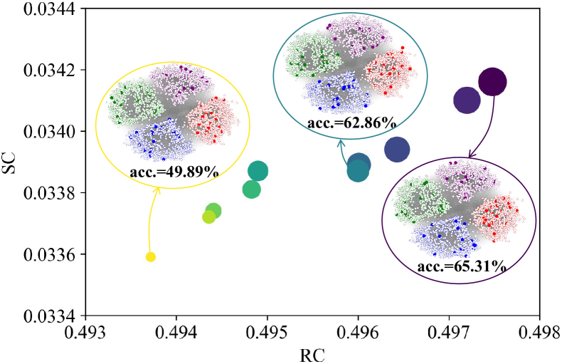
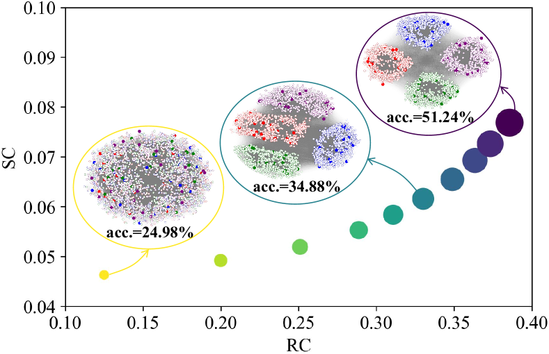
In Figure 2 and Figure 3, we show the relation between the reaching coefficient $RC$, the squashing coefficient $SC$, and the classification accuracy. The higher the accuracy, the darker and larger the corresponding scatter. First, we analyze the performance of GCN when trained on the same graph structure but with different labeled nodes. In Figure 2, we generate a synthetic graph by the Stochastic Block Model (SBM) (Holland et al., 1983) with 4 classes and 3,000 nodes. We randomly sample some nodes as the labeled nodes 10 times and scatter the classification accuracy in Figure 2. We can observe that even for the same graph structure, the difference in positions of labeled nodes may bring up to 15.42% difference in accuracy. There is a significant positive correlation between the reaching coefficient, the squashing coefficient, and the model performance.

Then we analyze the performance of GCN when trained with the same labeled nodes but on different graph structures. In Figure 3, we set the labeled nodes to be the same and generate different structures between them by controlling the edge probability between communities in the SBM model. We can observe that with the same supervision information, there is up to a 26.26% difference in accuracy because of the difference in graph structures. There is also a significant positive correlation between the reaching coefficient, the squashing coefficient, and the model performance. When the graph shows better community structure among nodes of the same class, the node representations can be learned better.

Therefore, we make the following conclusions: (1) Topology-imbalance hurts the performance of graph learning in the way of under-reaching and over-squashing. (for Q1) (2) The proposed two quantitative metrics can effectively reflect the degree of topology-imbalance. Graph with poor reachability (i.e., smaller $RC$) and stronger squashing (i.e., smaller $SC$) is more susceptible to topology-imbalance. (for Q2) (3) Optimizing the graph structure can effectively solve the topology-imbalance issue. The above conclusions provide the guideline for designing the framework of PASTEL, i.e., balance the supervision information distribution by learning a structure with better reachability and lower squashing.

4. Alleviate Topology-Imbalance by Structure Learning

In this section, we introduce PASTEL, a Position-Aware STructurE Learning framework, to optimize the information propagation path directly and address the topology-imbalance issue in essence. In light of the analysis in Section 3.2, PASTEL aims to learn a better structure that increases the intra-class label influence for each class and thus relieves the under-reaching and over-squashing phenomena. The overall architecture of PASTEL is shown in Figure 4.

4.1. Position-aware Structure Learning

To form structure with better intra-class connectivity, we use an anchor-based position encoding method to capture the topology distance between unlabeled nodes to labeled nodes. Then we incorporate both the merits of feature information as well as topology information to learn the refined structure.

Anchor-based Position Encoding. Inspired by the position in transformer (Vaswani et al., 2017; Shaw et al., 2018), we use an anchor-based position encoding method to capture the relative position of unlabeled nodes with respect to all the labeled nodes of the graph. Since we focus on maximizing the reachability between unlabeled nodes and labeled nodes within the same class, we directly separate the labeled node set $\mathcal{V}_{L}$ into $C$ anchor sets $\{\mathcal{V}^{1}_{L},\mathcal{V}^{2}_{L},\cdots,\mathcal{V}^{C}_{L}\}$, where each subset $\mathcal{V}^{c}_{L}$ denotes the labeled nodes whose labels are $c$. The class-wise anchor sets help distinguish the information from different classes rather than treating all the anchor nodes the same and ignoring the class difference as in (You et al., 2019). Concretely, for any node $v_{i}$, we consider a function $\phi(\cdot,\cdot)$ which measures the position relations between $v_{i}$ and the anchor sets in graph $\mathcal{G}$. The function can be defined by the connectivity between the nodes in the graph.

(4) $$\mathbf{p}_{i}=\left(\phi\left(v_{i},\mathcal{V}^{1}_{L}\right),\phi\left(v_{i},\mathcal{V}^{2}_{L}\right),\cdots,\phi\left(v_{i},\mathcal{V}^{C}_{L}\right)\right),$$

where $\phi(v_{i},\mathcal{V}^{c}_{L})$ is the position encoding function defined by the connectivity between the node $v_{i}$ and the anchor set $\mathcal{V}^{c}_{L}$ in graph. Here we choose $\phi(v_{i},\mathcal{V}^{c}_{L})$ to be the mean length of shortest path between $v_{i}$ and nodes in $\mathcal{V}^{c}_{L}$ if two nodes are connected:

(5) $$\phi(v_{i},\mathcal{V}^{c}_{L})=\frac{\sum_{v_{j}\in\mathcal{N}_{c}(v_{i})}|\mathcal{P}_{sp}(v_{i},v_{j})|}{|\mathcal{N}_{c}(v_{i})|},$$

where $\mathcal{N}_{c}(v_{i})$ is the nodes connected with $v_{i}$ in $\mathcal{V}^{c}_{L}$ and $|\mathcal{P}_{sp}(v_{i},v_{j})|$ is the length of shortest path between $v_{i}$ and $v_{j}$. Then we transform the position encoding into the $d_{0}$ dimensional space:

(6) $$\mathbf{h}^{p}_{i}=\mathbf{W}_{\phi}\cdot\mathbf{p}_{i},$$

where $\mathbf{W}_{\phi}$ is a trainable vector. If two nodes have similar shortest paths to the anchor sets, their position encodings are similar.

Figure 3. Predictions of GCN with and the same labeled nodes and different graph structures.

Figure 4. Overall architecture of PASTEL. PASTEL encodes the relative position between nodes with the labeled nodes as anchor sets {$\mathcal{S}$} and incorporates the position information with node features for structure learning. For each pair of nodes, PASTEL uses the class-wise conflict measure as the edge weights to learn a graph with better intra-class connectivity.

Position-aware Metric Learning. After obtaining the position encoding, we use a metric function that accounts for both node feature information and the position-based similarities to measure the possibility of edge existence. PASTEL is agnostic to various similarity metric functions and we choose the widely used multi-head cosine similarity function here:

(7) $$a^{P}_{ij}=\frac{1}{m}\sum^{m}_{h=1}\cos\left(\mathbf{W}_{h}\cdot\left(\mathbf{z}_{i}||\mathbf{h}^{p}_{i}\right),\mathbf{W}_{h}\cdot\left(\mathbf{z}_{j}||\mathbf{h}^{p}_{j}\right)\right),$$

where $m$ is the number of heads, $\mathbf{W}_{h}$ is the weight matrix of the $h$-th head, $\mathbf{z}_{i}$ denotes the representation vector of node $v_{i}$ and $||$ denotes concatenation. The effectiveness of the position-aware structure learning is evaluated in Section 5.3.1.

4.2. Class-wise Conflict Measure

We aim to increase the intra-class connectivity among nodes, thereby increasing the supervision information they received and their influence on each other. Here we propose a class-wise conflict measure to guide what nodes should be more closely connected. According to the inherent relation of GNNs with Label Propagation (Wang and Leskovec, 2021; Chen et al., 2021), we use the Group PageRank (Chen et al., 2020a) as a conflict measure between nodes. Group PageRank (GPR) extends the traditional PageRank(Page et al., 1999) into a label-aware version to measure the supervision information from labeled nodes of each class. Specifically, for class $c\in\{1,2,\cdots,C\}$, the corresponding GPR matrix is

(8) $$\mathbf{P}^{gpr}(c)=(1-\alpha)\mathbf{A}^{\prime}\mathbf{P}^{gpr}(c)+\alpha\mathbf{I}_{c},$$

where $\mathbf{A}^{\prime}=\mathbf{A}\mathbf{D}^{-1}$, $\alpha$ is the random walk restart probability at a random node in the group and $\mathbf{I}_{c}\in\mathbb{R}^{n}$ is the teleport vector:

(9) $$\mathbf{I}^{i}_{c}=\left\{\begin{matrix}\frac{1}{|\mathcal{V}^{c}_{L}|},&if~{}y_{i}=c\\ 0,&otherwise\end{matrix}\right.$$

where $|\mathcal{V}^{c}_{L}|$ is the number of labeled nodes with class $c$. We calculate the GPR for each group individually and then concatenate all the GPR vectors to form a final GPR matrix $\mathbf{P}^{gpr}\in\mathbb{R}^{N\times C}$ as in (Chen et al., 2020a):

(10) $$\mathbf{P}^{gpr}=\alpha\left(\mathbf{E}-\left(1-\alpha\right)\mathbf{A}^{\prime}\right)^{-1}\mathbf{I}^{*},$$

where $\mathbf{E}$ is the unit matrix of nodes and $\mathbf{I}^{*}$ is the concatenation of $\{\mathbf{I}_{c},c=1,2,\cdots,C\}$. Under $\mathbf{P}^{gpr}$, node $v_{i}$ corresponds to a GPR vector $\mathbf{P}^{gpr}_{i}$ (the $i$-th row of $\mathbf{P}^{gpr}$), where the $c$-th dimension represents the the supervision influence of labeled nodes of class $c$ on node $v_{i}$. The GPR value contains not only the global topology information but also the annotation information.

For each node pair nodes $v_{i}$ and $v_{j}$, we use the Kullback Leiber (KL) divergence of their GPR vectors to measure their conflict when forming an edge:

(11) $$\kappa_{ij}=\operatorname{KL}\left(\mathbf{P}^{gpr}_{i},\mathbf{P}^{gpr}_{j}\right).$$

The distance of GPR vectors reflects the influence conflict of different classes when exchanging information. We use a cosine annealing mechanism to calculate the edge weights by the relative ranking of the conflict measure:

(12) $$w_{ij}=\frac{1}{2}\left[-\cos{\frac{\operatorname{Rank}(\kappa_{ij})}{|\mathcal{V}|\times|\mathcal{V}|}*\pi}+1\right],$$

where $Rank(\cdot)$ is the ranking function according to the magnitude. The more conflicting the edge is, the less weight is assigned to it. With the class-wise conflict measure, we aim to learn a graph structure that makes the GPR vectors of nodes have “sharp” distributions focusing on their ground-truth classes. Then $w_{ij}$ is used as the connection strength of edge $e_{ij}$, with the corresponding element $\tilde{a}^{P}_{ij}$ in the adjacency matrix being:

(13) $$\tilde{a}^{P}_{ij}=w_{ij}\cdot a^{P}_{ij}.$$

The effectiveness of the class-wise conflict measure is evaluated in Section 5.3.2 and the change of GPR vectors is shown in Section 5.4.3.

Input: Graph $\mathcal{G}=\{\mathcal{V},\mathcal{E}\}$ with node labels $\mathcal{Y}$; Number of heads $m$; Number of training epochs $E$; Structure fusing coefficients $\lambda_{1},\lambda_{2}$; Loss coefficients $\beta_{1},\beta_{2},\beta_{3}$

Output: Optimized graph $\mathcal{G}^{*}=(\mathbf{A}^{*},\mathbf{X})$, predicted label $\hat{\mathcal{Y}}$

1 Parameter initialization;

2 for $e=1,2,\cdots,E$ do

       // Learn position-aware graph structure

3       Learn position encodings $\mathbf{h}^{p}_{i}$ $\leftarrow$ Eq. (6);

4       Learn edge possibility $a^{P}_{ij}$ $\leftarrow$ Eq. (7);

5       Calculate the Group PageRank matrix $\mathbf{P}^{gpr}\leftarrow$ Eq. (10);

6       Calculate the class-wise conflict measure $w_{ij}\leftarrow$ Eq. (12);

7       Obtain position-aware structure $\mathbf{A}_{P}$ $\leftarrow$ Eq. (14);

       // Learn node representations

8       Obtain the optimized structure $\mathbf{A}^{*}$ $\leftarrow$ Eq. (16);

9       Calculate representations and labels $\mathbf{Z}$, $\hat{\mathcal{Y}}$ $\leftarrow$ Eq. (20);

       // Optimize

10       Calculate the losses $\mathcal{L}_{cls}\leftarrow$ Eq. (21), $\mathcal{L}_{smooth}\leftarrow$Eq. (17), $\mathcal{L}_{con}\leftarrow$Eq. (18), and $\mathcal{L}_{spar}\leftarrow$Eq. (19);

11       Update model parameters to minimize $\mathcal{L}$ $\leftarrow$ Eq. (22).

12 end for

Algorithm 1 The overall process of PASTEL

4.3. Learning with the Optimized Structure

With the above structure learning strategy, we can obtain a position-aware adjacency $\mathbf{A}_{P}$ with maximum intra-class connectivities:

(14) $$\mathbf{A}_{P}=\{\tilde{a}^{P}_{ij},i,j\in\{1,2,\cdots,N\}\}.$$

The input graph structure determines the learning performance to a certain extent. Since the structure learned at the beginning is of poor quality, directly using it may lead to non-convergence or unstable training of the whole framework. We hence incorporate the original graph structure $\mathbf{A}$ and a structure in a node feature view $\mathbf{A}_{N}$ as supplementary to formulate an optimized graph structure $\mathbf{A}^{*}$. Specifically, we also learn a graph structure $\mathbf{A}_{N}=\{a^{N}_{ij},i,j\in\{1,2,\cdots,N\}\}$ in a node feature view with each element being:

(15) $$a^{N}_{ij}=\frac{1}{m}\sum^{m}_{h=1}\cos\left(\mathbf{W}_{h}\cdot\left(\mathbf{x}_{i}||\mathbf{h}^{p_{0}}_{i}\right),\mathbf{W}_{h}\cdot\left(\mathbf{x}_{j}||\mathbf{h}^{p_{0}}_{j}\right)\right),$$

where $\mathbf{x}_{i}$ is the feature vector of node $v_{i}$ and $\mathbf{h}^{p_{0}}_{i}$ is the position encoding with the original structure. Then we can formulate an optimized graph structure $\mathbf{A}^{*}$ with respect to the downstream task:

(16) $$\mathbf{A}^{*}=\lambda_{1}\mathbf{D}^{-\frac{1}{2}}\mathbf{A}\mathbf{D}^{-\frac{1}{2}}+\left(1-\lambda_{1}\right)\left(\lambda_{2}f\left(\mathbf{A}_{N}\right)+\left(1-\lambda_{2}\right)f\left(\mathbf{A}_{P}\right)\right),$$

where $f(\cdot)$ denotes the row-wise normalization function, $\lambda_{1}$ and $\lambda_{2}$ are two constants that control the contributions of original structure and feature view structure, respectively. Here we use a dynamic decay mechanism for $\lambda_{1}$ and $\lambda_{2}$ to enable the position-aware structure $\mathbf{A}_{P}$ to play a more and more important role during training.

To control the quality of learned graph structure, we impose additional constraints on it following (Kalofolias, 2016; Chen et al., 2020b) in terms of smoothness, connectivity, and sparsity:

(17) $$\mathcal{L}_{smooth} =\frac{1}{N^{2}}{\rm tr}\left(\mathbf{X}^{T}\mathbf{L}^{*}\mathbf{X}\right),$$

(18) $$\mathcal{L}_{con} =\frac{1}{N}\mathbf{1}^{T}\log(\mathbf{A}^{*}\mathbf{1}),$$

(19) $$\mathcal{L}_{spar} =\frac{1}{N^{2}}||\mathbf{A}^{*}||^{2}_{F},$$

where $\mathbf{L}^{*}=\mathbf{D}^{*}-\mathbf{A}^{*}$ is the Laplacian of $\mathbf{A}^{*}$ and $\mathbf{D}^{*}$ is the degree matrix of $\mathbf{A}^{*}$. To speed up the computation, we extract a symmetric sparse non-negative adjacency matrix by masking off (i.e., set to zero) those elements in $\mathbf{A}^{*}$ which are smaller than a predefined non-negative threshold $a_{0}$. Then $\mathcal{G}^{*}=(\mathbf{A}^{*},\mathbf{X})$ is input into the $\operatorname{GNN-Encoder}$ for the node representations $\mathbf{Z}\in\mathbb{R}^{N\times d}$, predicted labels $\hat{y}$ and classification loss $\mathcal{L}_{cls}$:

(20) $$\mathbf{Z}=\operatorname{GNN-Encoder}(\mathbf{A}^{*},\mathbf{X}),\hat{\mathcal{Y}}=\operatorname{Classifier}(\mathbf{Z}),$$

(21) $$\mathcal{L}_{cls}=\operatorname{Cross-Entropy}(\mathcal{Y},\hat{\mathcal{Y}}).$$

The overall loss is defined as the combination of the node classification loss and graph regularization loss:

(22) $$\mathcal{L}=\mathcal{L}_{cls}+\beta_{1}\mathcal{L}_{smooth}+\beta_{2}\mathcal{L}_{con}+\beta_{3}\mathcal{L}_{spar}.$$

The overall process of PASTEL is shown in Algorithm 1.

5. Experiment

In this section, we first evaluate PASTEL on both real-world graphs and synthetic graphs. Then we analyze the main mechanisms of PASTEL and the learned structure. We mainly focus on the following research questions:

• RQ1. How does PASTEL perform in the node classification task? (Section 5.2)

• RQ2. How does the position encoding and the class-wise conflict measure influence the performance of PASTEL? (Section 5.3)

• RQ3. What graph structure PASTEL tend to learn? (Section 5.4)

5.1. Experimental Setups

Table 1. Weighted-F1 score and Macro-F1 score (% ± standard deviation) of node classification on real-world graph datasets.

Cora

Citeseer

Photo

Actor

Chameleon

Squirrel

Backbone

Model

W-F1

M-F1

W-F1

M-F1

W-F1

M-F1

W-F1

M-F1

W-F1

M-F1

W-F1

M-F1

GCN

original

79.4±0.9

77.5±1.5

66.3±1.3

62.2±1.2

85.4±2.8

84.6±1.3

21.8±1.3

20.9±1.4

30.5±3.4

30.5±3.3

21.9±1.2

21.9±1.2

ReNode

80.0±0.7

78.4±1.3

66.4±1.0

62.4±1.1

86.2±2.4

85.3±1.6

21.2±1.2

20.2±1.6

30.3±3.2

30.4±2.8

22.4±1.1

22.4±1.1

AddEdge

79.0±0.9

77.0±1.4

66.2±1.3

62.2±1.3

85.5±1.5

86.1±1.8

21.2±1.3

20.3±1.5

30.6±1.6

30.4±1.7

21.7±1.5

21.7±1.5

DropEdge

79.8±0.8

77.8±1.0

66.6±1.4

63.4±1.6

86.8±1.7

85.4±1.3

22.4±1.0

21.4±1.3

30.6±3.5

30.6±3.3

22.8±1.2

22.8±1.2

SDRF

82.1±0.8

80.6±0.8

69.6±0.4

66.6±0.3

¿ 5 days

¿ 5 days

¿ 5 days

¿ 5 days

39.1±1.2

39.0±1.2

¿ 5 days

¿ 5 days

NeuralSparse

81.7±1.4

80.9±1.4

71.8±1.2

69.0±1.0

89.7±1.9

88.7±1.8

24.4±1.5

23.6±1.6

44.9±3.0

44.9±2.8

28.1±1.8

28.1±1.8

IDGL

82.3±0.6

81.0±0.9

71.7±1.0

68.0±1.3

88.6±2.3

88.8±1.4

24.9±0.8

22.0±0.7

55.4±1.8

55.0±1.7

28.8±2.3

28.9±2.2

PASTEL

82.5±0.3

81.2±0.3

72.9±0.8

69.3±0.9

91.4±2.7

91.3±2.2

26.4±1.0

24.4±1.2

57.8±2.4

57.3±2.4

37.5±0.6

37.5±0.7

GAT

original

78.3±1.5

76.4±1.7

64.4±1.7

60.6±1.7

88.2±2.9

86.2±2.6

21.8±1.2

20.9±1.1

29.9±3.5

29.9±3.1

20.5±1.4

20.5±1.4

ReNode

78.9±1.2

77.2±1.5

64.9±1.6

61.0±1.5

89.1±2.4

87.1±2.6

21.5±1.2

20.5±1.1

29.2±2.3

29.1±2.0

20.4±1.8

20.4±1.8

AddEdge

78.0±1.6

76.2±1.6

64.0±1.3

60.2±1.3

88.2±2.4

86.2±2.5

21.3±1.2

20.3±1.1

29.8±1.7

29.6±1.5

20.7±1.6

20.7±1.6

DropEdge

78.7±1.3

76.9±1.5

64.5±1.4

60.5±1.3

88.9±1.9

87.1±2.1

22.9±1.2

21.8±1.1

30.3±1.6

30.2±1.2

21.2±1.5

21.2±1.5

SDRF

77.9±0.7

75.9±0.9

64.9±0.6

61.9±0.9

¿ 5 days

¿ 5 days

¿ 5 days

¿ 5 days

43.0±1.9

42.5±1.9

¿ 5 days

¿ 5 days

NerualSparse

81.4±4.8

79.4±4.8

64.8±1.5

61.9±1.3

90.2±2.5

88.0±2.3

23.4±1.7

22.4±1.5

45.6±2.1

45.5±1.8

28.8±1.3

28.8±1.3

IDGL

80.6±1.0

79.7±0.9

66.5±1.5

61.9±1.9

89.9±3.1

87.7±2.6

22.4±1.5

21.8±1.2

48.4±4.0

47.8±3.1

27.0±2.6

27.0±2.6

PASTEL

81.9±1.4

80.7±1.2

66.6±1.9

62.0±1.7

91.8±3.2

89.4±2.9

24.4±2.6

22.1±2.6

52.1±2.7

52.5±2.8

35.3±0.9

35.3±0.8

APPNP

original

80.6±1.6

79.3±1.2

66.5±1.5

62.3±1.5

89.3±1.6

86.3±1.7

21.1±1.5

20.7±1.1

35.3±4.0

35.0±3.8

23.1±1.6

23.1±1.6

ReNode

81.1±0.9

79.9±0.9

66.6±1.7

62.4±1.6

89.6±1.4

87.2±1.3

20.2±2.0

20.0±1.7

33.5±2.5

33.3±2.3

23.9±2.0

23.9±2.0

AddEdge

80.3±1.3

78.8±1.1

66.6±2.1

62.5±2.1

89.3±1.2

86.4±1.2

21.5±1.3

20.7±1.4

35.7±1.7

35.4±1.2

23.1±1.6

23.2±1.7

DropEdge

80.9±1.4

79.4±1.2

66.7±2.0

63.0±1.9

90.0±1.2

87.0±1.2

21.8±1.8

20.8±1.4

36.0±1.7

35.7±1.6

23.3±1.7

23.3±1.7

SDRF

80.7±0.9

79.1±0.8

67.1±0.6

63.1±0.8

¿ 5 days

¿ 5 days

¿ 5 days

¿ 5 days

36.5±2.1

35.8±2.1

¿ 5 days

¿ 5 days

NerualSparse

81.1±1.4

79.9±1.2

66.8±1.9

62.7±1.9

91.3±1.8

89.4±1.6

21.8±1.9

21.4±1.5

39.1±2.9

38.7±2.8

28.3±1.5

28.3±1.5

IDGL

81.3±0.9

80.2±0.9

67.0±1.3

62.9±1.3

91.6±1.3

88.6±2.2

21.4±2.4

20.1±2.4

41.2±2.2

40.6±2.6

29.6±2.3

29.7±2.2

PASTEL

82.0±1.0

80.0±0.9

67.3±1.3

63.2±1.5

92.3±3.1

89.9±2.5

22.5±2.0

20.9±2.1

44.2±3.2

43.8±3.4

34.6±1.6

34.6±1.6

GraphSAGE

original

75.4±1.6

74.1±1.6

64.8±1.6

60.7±1.6

86.1±2.5

83.3±2.4

24.0±1.2

23.2±1.0

36.5±1.6

36.2±1.6

27.2±1.7

27.2±1.7

ReNode

76.4±0.9

75.0±1.1

65.4±1.7

61.2±1.7

86.5±1.7

84.1±1.7

23.7±1.2

22.8±1.0

36.4±1.9

36.1±1.9

27.7±1.8

27.7±1.8

AddEdge

75.2±1.2

73.7±1.2

65.0±1.4

60.9±1.3

86.1±2.8

83.4±2.6

23.8±1.7

23.2±1.6

36.5±1.5

36.2±1.3

26.9±2.1

26.9±2.1

DropEdge

76.0±1.6

74.5±1.6

65.1±1.4

60.9±1.4

86.2±1.6

83.5±1.4

24.1±1.0

23.3±0.9

37.5±1.4

37.2±1.4

27.5±1.8

27.5±1.8

SDRF

75.7±0.8

74.6±0.8

65.3±0.6

61.4±0.6

¿ 5 days

¿ 5 days

¿ 5 days

¿ 5 days

41.5±2.6

41.6±2.7

¿ 5 days

¿ 5 days

NerualSparse

79.7±1.8

77.8±1.6

64.7±1.4

61.1±1.3

89.1±5.4

86.7±5.5

25.1±1.2

24.4±1.1

39.1±1.9

39.0±1.9

32.2±2.4

32.2±2.4

IDGL

79.2±0.9

78.4±0.8

65.6±0.9

61.3±1.2

90.0±1.0

86.3±1.3

24.0±2.6

22.4±2.7

43.8±3.4

43.0±3.2

33.9±0.9

33.9±0.8

PASTEL

81.1±0.8

79.8±0.7

65.7±1.1

61.4±1.4

92.0±0.6

89.0±1.0

26.0±2.4

23.6±2.7

47.7±0.9

46.9±0.9

35.5±1.4

35.5±1.4

5.1.1. Datasets

We conduct experiments on synthetic and real-world datasets to analyze the model’s capabilities in terms of both graph theory and real-world scenarios. The real-word datasets include various networks with different heterophily degrees to demonstrate the generalization of PASTEL. Cora and Citeseer (Sen et al., 2008) are citation networks. Photo (Shchur et al., 2018) and and Actor (Pei et al., 2020) are co-occurrence network. Chameleon and Squirrel (Rozemberczki et al., 2021) are page-page networks in Wikipedia. Since we focus on the topology-imbalance issue in this work, we set the number of labeled nodes in each class to be 20.

5.1.2. Baselines

We choose representative GNNs as backbones including GCN (Kipf and Welling, 2017), GAT (Veličković et al., 2017), APPNP (Klicpera et al., 2019), and GraphSAGE (Hamilton et al., 2017). The most important baseline is ReNode (Chen et al., 2021), which is the only existing work for the topology-imbalance issue. We also include some graph structure learning baselines to illustrate the specific effectiveness of PASTEL for the topology-imbalance issue. DropEdge (Rong et al., 2019) randomly removes edges at each epoch as structure augmentation. To evaluate the effect of increasing the reachability randomly, we use a adding edges method named AddEdge, whose adding strategy is similar to DropEdge. SDRF (Topping et al., 2022) rewires edges according to their curvatures for the over-squashing issue. NeuralSparse (Zheng et al., 2020) removes potentially task-irrelevant edges for clearer class boundaries. IDGL (Chen et al., 2020b) updates the node representations and structure based on these representations iteratively.

5.1.3. Parameter Settings

For the GNN backbones, we set their depth to be 2 layers and adopt the implementations from the PyTorch Geometric Library in all experiments. We set the representation dimension of all baselines and PASTEL to be 256. We re-implement the NeuralSparse (Zheng et al., 2020) and SDRF (Topping et al., 2022) and the parameters of baseline methods are set as the suggested value in their papers or carefully tuned for fairness. For DropEdge and AddEdge, we set the edge dropping/adding probability to 10%. For PASTEL, we set the number of heads $m=4$ and the random walk restart probability $\alpha=0.15$. The structure fusing coefficients ($\lambda_{1}$ and $\lambda_{2}$) and the loss coefficients ($\beta_{1}$, $\beta_{2}$ and $\beta_{3}$) are tuned for each dataset.

5.2. Evaluation (RQ1)

Table 2. Weighted-F1 scores and improvements on graphs with different levels of topology-imbalance.

	Cora-L		Cora-M		Cora-H
	$RC$ 0.4130	$SC$ -0.6183	$RC$ 0.4100	$SC$ -0.6204	$RC$ 0.4060	$SC$ -0.6302
	W-F1 (%)	$\Delta$ (%)	W-F1 (%)	$\Delta$ (%)	W-F1 (%)	$\Delta$ (%)
GCN	80.9±0.9	—	78.8±0.8	—	77.5±1.0	—
ReNode	81.3±0.7	$\uparrow$0.4	79.3±0.8	$\uparrow$0.5	78.3±1.1	$\uparrow$0.8
SDRF	81.0±0.7	$\uparrow$0.1	78.9±0.8	$\uparrow$0.1	77.9±0.7	$\uparrow$0.4
IDGL	82.5±1.0	$\uparrow$1.6	80.4±1.0	$\uparrow$1.6	81.6±1.1	$\uparrow$4.1
PASTEL	82.7±0.9	$\uparrow$1.8	81.0±0.9	$\uparrow$2.2	81.9±1.1	$\uparrow$4.4

5.2.1. PASTEL for Real-world Graphs

We compare PASTEL with the baselines on several datasets on node classification. The overall Weighted-F1 (W-F1) scores and the class-balance Macro-F1 (M-F1) scores on different backbones are shown in Table 1. The best results are shown in bold and the runner-ups are underlined. PASTEL shows overwhelming superiority in improving the performance of backbones on all datasets. It demonstrates that PASTEL is capable of learning better structures with a more balanced label distribution that reinforces the GNN models. ReNode (Chen et al., 2021) achieves fewer improvements on datasets of poor connectivity (e.g., CiteSeer) and even damages the performance of backbones on heterophilic datasets (e.g., Chameleon and Actor). We think it’s because ReNode (Chen et al., 2021) detects conflicts by Personalized PageRank and fails to reflect the node topological position well when the graph connectivity is poor. Besides, ReNode takes the topology boundary as the decision boundary, which is not applicable for heterophilic graphs. AddEdge doesn’t work in most cases, demonstrating that randomly adding edge is not effective in boosting the reachability. The structure augmentation strategy should be carefully designed considering the node relations. SDRF (Topping et al., 2022) can improve the performance, supporting our intuition that relieving over-squashing helps graph learning. But SDRF is still less effective than PASTEL because it only considers the topological properties rather than the supervision information. Both NeuralSparse (Zheng et al., 2020) and IDGL (Chen et al., 2020b) show good performance among the baselines, showing the effectiveness of learning better structures for downstream tasks. However, they are still less effective than PASTEL which takes the supervision information distribution into consideration.

Table 3. Weighted-F1 scores (%) and improvements ($\Delta$) on synthetic SBM graphs with different community structures.

	SBM-1		SBM-2		SBM-3		SBM-4		SBM-5		SBM-6		SBM-7
$p$	0.5000		0.5000		0.5000		0.5000		0.5000		0.5000		0.5000
$q$	0.0300		0.0100		0.0083		0.0071		0.0063		0.0056		0.0050
$RC$	0.4979		0.4984		0.4990		0.4994		0.5002		0.5004		0.5009
$SC$	0.0998		0.0999		0.1000		0.1001		0.1007		0.1017		0.1144
	W-F1	$\Delta$	W-F1	$\Delta$	W-F1	$\Delta$	W-F1	$\Delta$	W-F1	$\Delta$	W-F1	$\Delta$	W-F1	$\Delta$
GCN	40.29	—	42.37	—	42.99	—	44.13	—	45.19	—	45.21	—	45.22	—
ReNode	41.33	$\uparrow$1.04	42.40	$\uparrow$0.03	43.21	$\uparrow$0.22	44.56	$\uparrow$0.43	45.20	$\uparrow$0.01	45.08	$\downarrow$0.13	44.89	$\downarrow$0.33
PASTEL	45.67	$\uparrow$5.38	57.61	$\uparrow$15.24	58.33	$\uparrow$15.34	60.29	$\uparrow$16.16	66.41	$\uparrow$21.22	66.45	$\uparrow$21.24	66.57	$\uparrow$21.35

5.2.2. PASTEL under Different Levels of Topology-imbalance

To further analyze PASTEL’s ability in alleviating the topology-imbalance issue, we verify the PASTEL under different levels of topology-imbalance. We randomly sampled 1,000 training sets and calculate the reaching coefficient $RC$ and squashing coefficient $SC$ as introduced in Section 3.2. Then we choose 3 training sets with different levels of topology-imbalance according to the conclusion in Section 3.3 and we denote them as Cora-L, Cora-M, and Cora-H, according to the degree of topology imbalance. Note that larger $RC$ means better reachability and larger $SC$ means lower squashing. We evaluate PASTEL and several baselines with the GCN as the backbone and show the dataset information, the Weighted-F1 scores, and their improvements ($\Delta$) over the backbones in Table 2. The performance of node representation learning generally gets worse with the increase of the topology-imbalance degree of the dataset. Both the node re-weighting method (i.e., ReNode (Chen et al., 2021)) and the structure learning methods (i.e., IDGL (Chen et al., 2020b), SDRF (Topping et al., 2022) and PASTEL) can achieve more improvement with the increase of dataset topology-imbalance. PASTEL performs best on all datasets with different degrees of topology-imbalance and it can achieve up to 4.4% improvement on the highly topology-imbalance dataset.

5.2.3. PASTEL for Synthetic Graphs

Figure 5. The impact of position encoding.

We generate 7 synthetic graph datasets with different community structures using the Stochastic Block Model (SBM) $\mathcal{G}(N,C,p,q)$ (Holland et al., 1983), where the number of nodes $N=3000$, the number of community $C=6$, $p$ denotes the edge probability within a community and $q$ denotes the edge probability between communities. We show the classification Weighted-F1 scores and improvements are shown in Table 3. With a more clear community structure, the reaching coefficient $RC$ increases and the squashing coefficient $SC$ also increases, leading to the increase of GCN’s performance, which agrees with the conclusion obtained in Section 3.3. ReNode shows unsatisfied performance in boosting the node classification. PASTEL can increase the classification weighted-F1 score by 5.38%-21.35% on SBM graphs with different community structures, showing superior effectiveness.

5.3. Analysis of PASTEL (RQ2)

We conduct ablation studies for the two main mechanisms of PASTEL, position encoding and class-wise conflict measure.

5.3.1. Impact of the Position Encoding

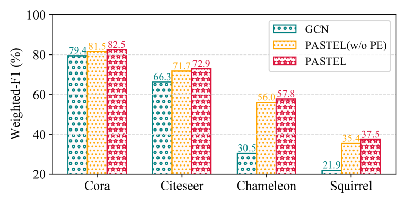
We design an anchor-based position encoding mechanism in Section 4.1, which reflects the relative topological position to labeled nodes and further maximizes the label influence within a class. To evaluate the effectiveness of position encoding, we compare PASTEL with a variant PASTEL (w/o PE), which removes the position encoding and directly take the node features for metric learning in Eq. (7).

Figure 6. The impact of class-wise conflict measure.

Here we use the GCN as the backbone. As shown in Figure 5, the structure learning strategy of PASTEL contributes the most, which can achieve at most 25.5% improvement in terms of Weighted-F1 score with only node features. Although PASTEL (w/o PE) effectively improves the performance of backbones to some extent, the position encoding still benefits learning better structure to relieve the topology-imbalance with 1.0%-1.8% improvements than PASTEL (w/o PE).

(a) Original Graph.

(b) ReNode.

(c) SDRF.

(d) IDGL.

(e) PASTEL.

Figure 7. Structure visualization. (a) Original graph of Cora and learned graphs by (b) ReNode, (c) SDRF, (d) IDGL and (e) PASTEL.

5.3.2. Impact of the Class-wise Conflict Measure

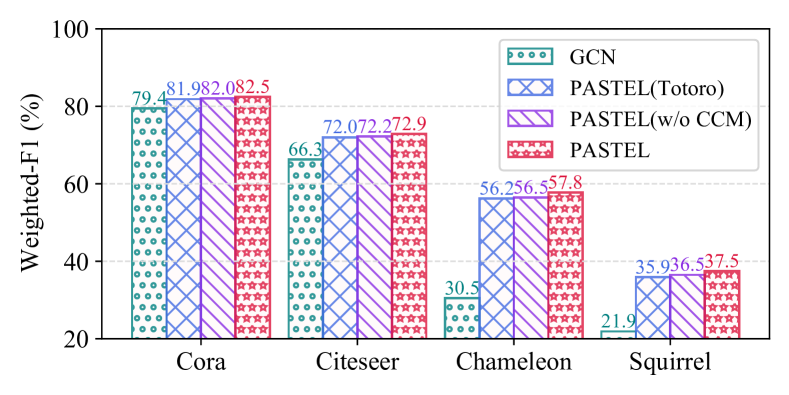
We designed a class-wise conflict measure in Section 4.2 as edge weights to guide learning structures with better intra-class connectivity. Here, we compare PASTEL with its two variants to analyze the impact of the class-wise conflict measure: (1) PASTEL (w/o CCM), which removes the class-wise conflict measure and directly takes the learned edge possibilities in Eq. (7) as the edge weights. (2) PASTEL (Totoro), which takes the Totoro metric introduced in ReNode (Chen et al., 2021) as the conflict measure of nodes in Eq. (13). Here we use the GCN as the backbone. The comparison results are shown in Figure 6. On four datasets, PASTEL consistently outperforms the other two variants. Even without the conflict measure, PASTEL (w/o CCM) still shows better performance than PASTEL (Totoro), indicating the limitation of ReNode when capturing the relative topology positions without clear homophily structures.

5.4. Analysis of Learned Structure (RQ3)

We analyze the learned graph by PASTEL in terms of visualization and structural properties.

5.4.1. Structure Visualization

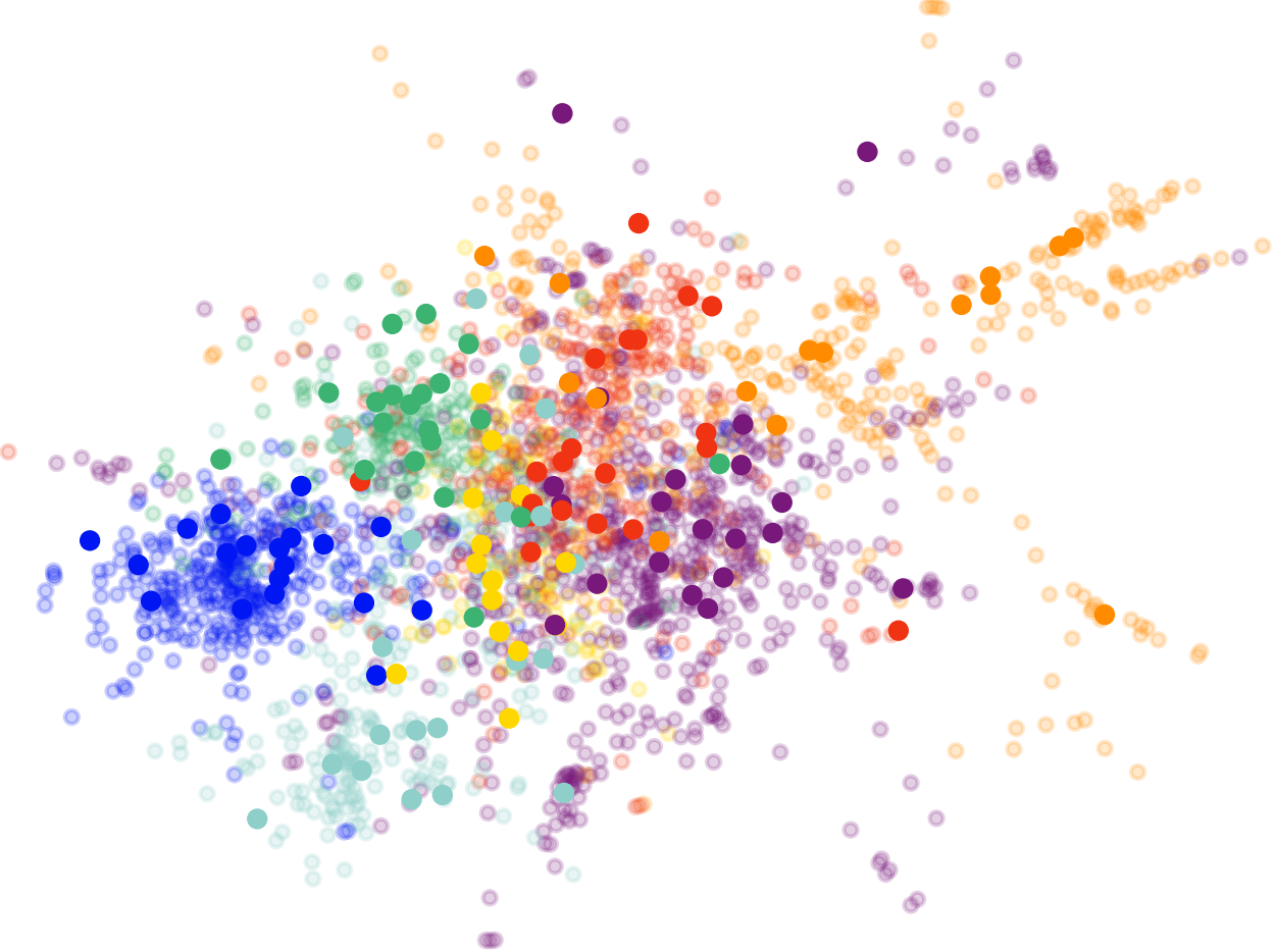
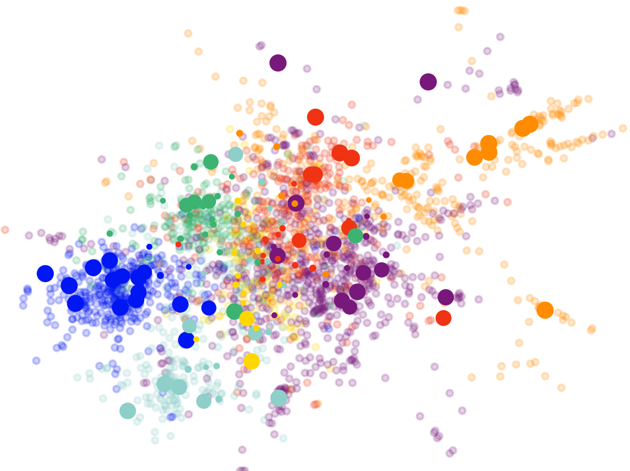
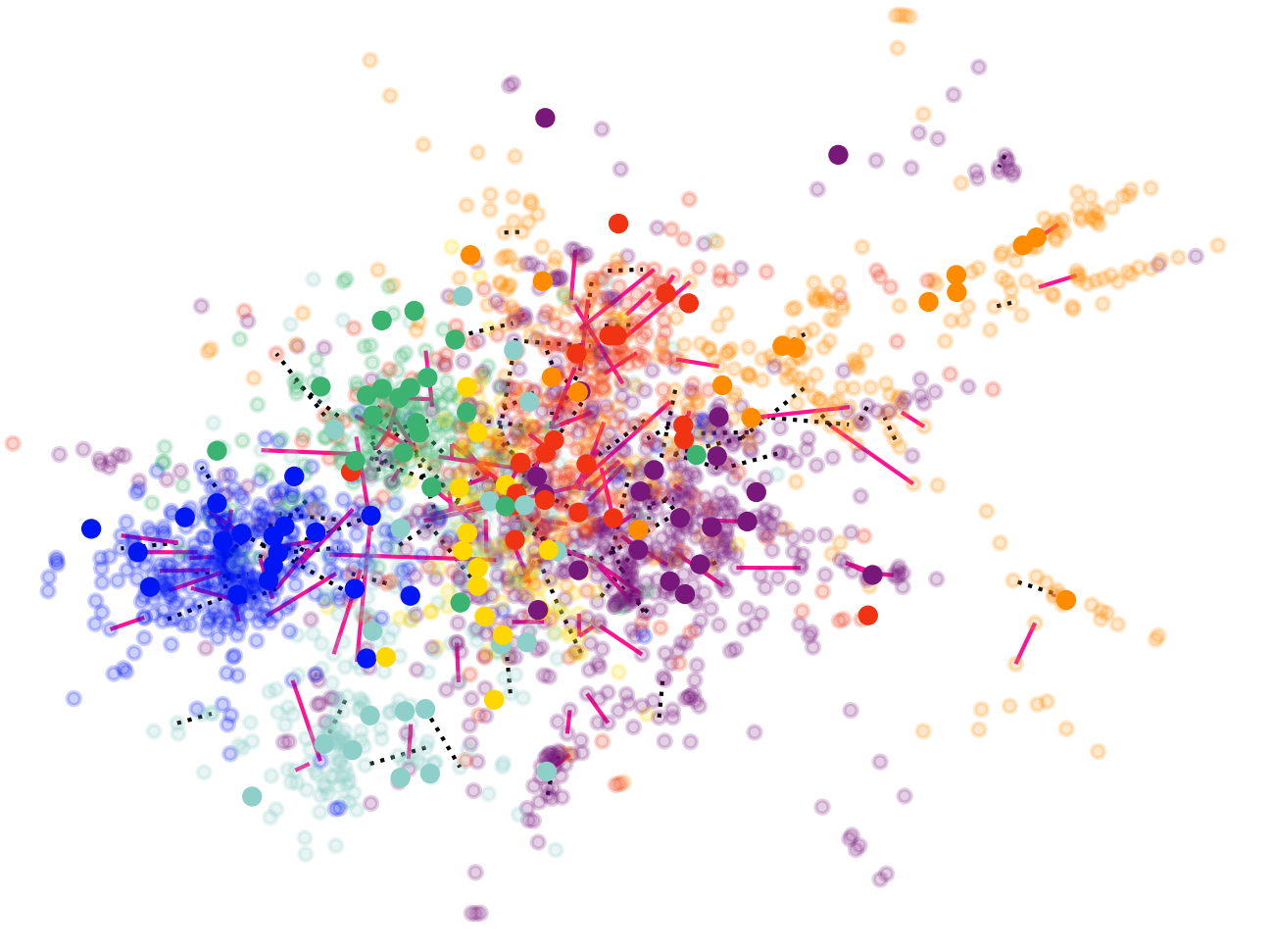
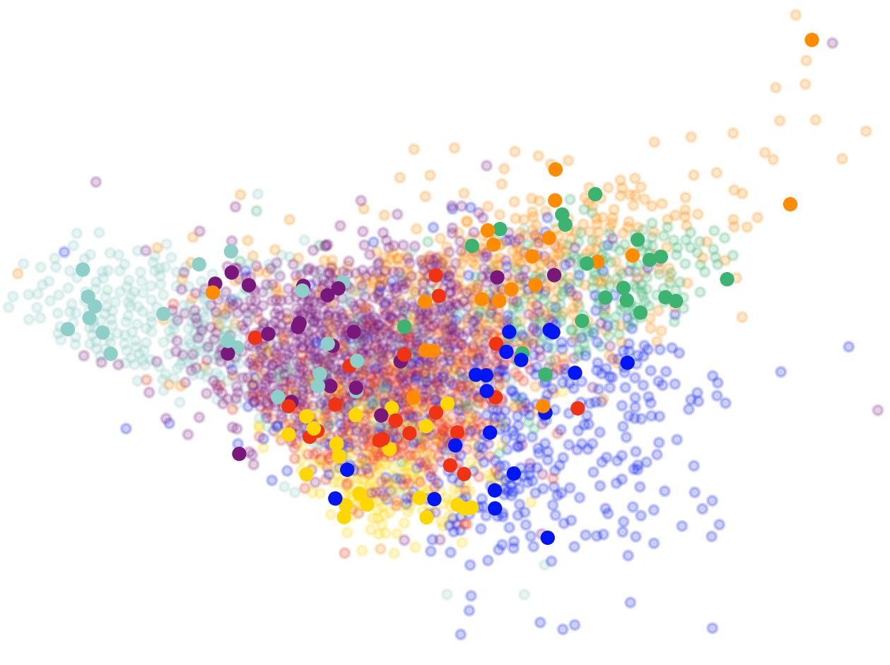
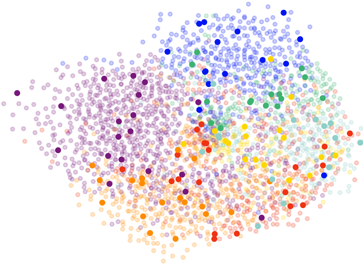
In Figure 7, we visualize the original graph of Cora and the graphs learned by ReNode (Chen et al., 2021), SDRF (Topping et al., 2022), IDGL (Chen et al., 2020b) and PASTEL using networkx. For clarity, the edges are not shown. The solid points denote the labeled nodes, the hollow points denote the unlabeled nodes, and the layout of nodes denotes their connectivities. The node size in Figure 7(b) denotes the learned node weight in ReNode, and the solid lines and dashed lines in Figure 7(c) denote the added and deleted edges by SDRF, respectively. As we can observe, ReNode gives more weights to nodes in the topology center of each class and SDRF tends to build connections between distant or isolated nodes. Even though the structure learned by IDGL can make the nodes of a class close, there are still some overlapping and entangled areas between classes. Benefiting from the position encoding and class-wise conflict measure, PASTEL can obtain graph structure with clearer class boundaries.

Table 4. Properties and performance of the original graph and learned graphs of Cora.

	Original Graph	ReNode	SDRF	IDGL	PASTEL
$RC$	0.4022	0.4022	0.4686	0.5028	0.5475
$SC$	-0.6299	-0.6299	-0.4942	-0.4069	-0.3389
W-F1 (%)	79.44	80.34	82.01	82.38	82.86

5.4.2. Change of $RC$ and $SC$

We also show the reaching coefficient $RC$ and the squashing coefficient $SC$ of the above graphs in Figure 7 and the Weighted-F1 score learned on them in Table 4. Here we choose the GCN as the model backbone. All of the structure learning methods (SDRF (Topping et al., 2022), IDGL (Chen et al., 2020b) and PASTEL) learn structures with larger reaching coefficient and larger squashing coefficient, leading the performance improvement of node classification. This phenomenon supports our propositions in Section 3.3 again.

5.4.3. Change of GPR Vector

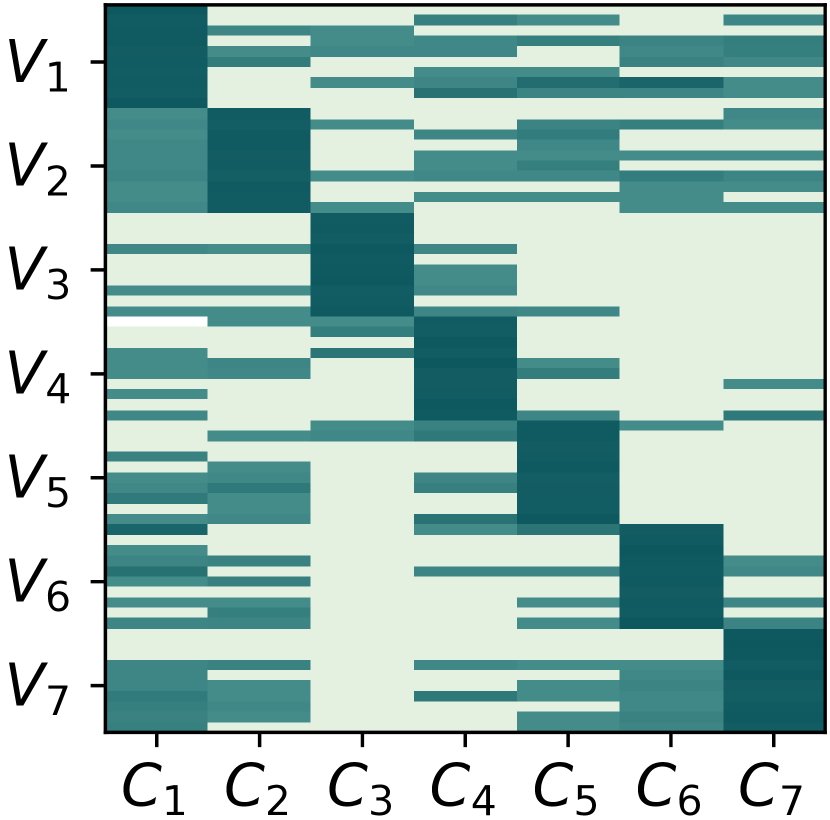
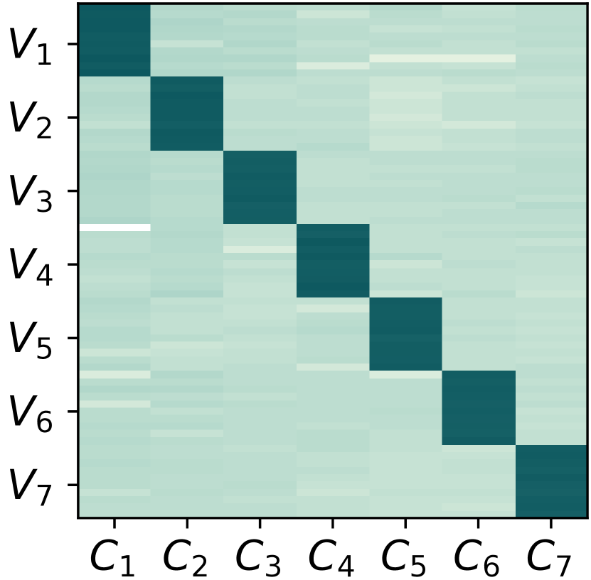
The class-wise conflict measure is calculated by the Group PageRank (GPR), which reflects the label influence of each class. We randomly choose 10 nodes for each class in Cora and show their GPR vectors $\mathbf{P}^{gpr}_{i}$ in the original graph in Figure 8(a) and the learned graph in Figure 8(b), respectively, where the color shade denotes the magnitude, $V_{i}$ denotes 10 nodes of class $i$ and $C_{i}$ denotes the $i$-th class. In Figure 8(a), the off-diagonal color blocks are also dark, indicating that the label influence of each class that nodes obtained from the original graph is still entangled to some extent, which could bring difficulties to the GNN optimization. After the structure learning guided by the proposed class-wise conflict measure, Figure 8(b) exhibits 7 clear diagonal blocks and the gaps between the diagonal and off-diagonal block are widened, indicating that nodes can receive more supervision information of its ground-truth class. We can further make a conclusion that the class-wise conflict measure plays an important role on giving guidance for more class connectivity orthogonality.

(a) Original Graph.

(b) Learned Graph.

Figure 8. Heat maps for the Group PageRank value of (a) the original graph and (b) the learned graph by PASTEL.

6. Conclusion

We proposed a novel framework named PASTEL for the graph topology-imbalance issue. We provide a new understanding and two quantitative analysis metrics of topology-imbalance in the perspective of under-reaching and over-squashing, answering the questions that how topology-imbalance affects GNN’s performance as well as what graphs are susceptible to it. PASTEL designs an anchor-based position encoding mechanism and a class-wise conflict measure to obtain structures with better in-class connectivity. Comprehensive experiments demonstrate the potential and adaptability of PASTEL. An interesting future direction is to incorporate the proposed two quantitative metrics into the learning process to address topology-imbalance more directly.