Last-iterate Convergence to Trembling-hand Perfect Equilibria

Martino Bernasconi
Politecnico di Milano
martino.bernasconideluca@polimi.it &Alberto Marchesi
Politecnico di Milano
alberto.marchesi@polimi.it &Francesco Trovò
Politecnico di Milano
francesco1.trovo@polimi.it
Abstract

Designing efficient algorithms to find Nash equilibrium (NE) refinements in sequential games is of paramount importance in practice. Indeed, it is well known that the NE has several weaknesses, since it may prescribe to play sub-optimal actions in those parts of the game that are never reached at the equilibrium. NE refinements, such as the extensive-form perfect equilibrium (EFPE), amend such weaknesses by accounting for the possibility that players may make mistakes. This is crucial in real-world applications, where humans having bounded rationality are usually involved, and it turns out being useful also in boosting the performances of superhuman agents for recreational games like Poker. Nevertheless, only few works addressed the problem of computing NE refinements. Most of them propose algorithms finding exact NE refinements by means of linear programming, and, thus, these do not have the potential of scaling up to real-world-size games. On the other hand, existing iterative algorithms that exploit the tree structure of sequential games only provide convergence guarantees to approximate refinements. In this paper, we provide the first efficient last-iterate algorithm that provably converges to an EFPE in two-player zero-sum sequential games with imperfect information. Our algorithm works by tracking a sequence of equilibria of suitably-defined, regularized-perturbed games. In order to do that, it uses a procedure that is specifically tailored to converge last iterate to the equilibria of such games. Crucially, the updates performed by such a procedure can be performed efficiently by visiting the game tree, thus rendering our algorithm more appealing than its linear-programming-based competitors in terms of scalability. Finally, we evaluate our algorithm on a standard testbed of games, showing that it outputs strategies which are much more robust to players’ mistakes than those of state-of-the-art NE-computation algorithms.

1 Introduction

Computing the Nash equilibria (NEs) (Nash, 1951) of two-player zero-sum sequential (i.e., extensive-form) games with imperfect information has been one of the flagship computational challenges of artificial intelligence since several years. The latest advances in such a research field have lead to the development of superhuman agents that are capable of beating top human professionals in several recreational games, such as, e.g., Go (Silver et al., 2016) and heads-up no-limit Texas hold’em Poker (Brown and Sandholm, 2018, 2019).

The NE is a solution concept that prescribes each player to play optimally under the assumption that the opponents are perfectly rational and do the same. However, this assumption is oftentimes unreasonable, especially when computed equilibria are deployed in the real world, where artificial agents usually face human opponents that naturally have bounded rationality. Moreover, it is well known that the NE has several weaknesses when played against opponents with bounded rationality who may make mistakes. In particular, an NE may prescribe to perform sub-optimal actions at decision points (a.k.a. information sets) that are never reached assuming the players play equilibrium strategies.

Over the last decades, game theorists introduced several refinements of the NE notion, in order to amend its weaknesses off the equilibrium path. Among them, the most studied one is the extensive-form perfect equilibrium (EFPE) introduced by Selten (1975). The EFPE is based on the idea of trembling-hand perfection, whose rationale is to let the players reasoning about the possibility that both themselves and their opponents may “tremble” in future, by playing sub-optimal actions with small probability at information sets that will be reached later during the game. Then, an EFPE is defined as a limit point of a sequence of equilibria that is obtained by letting the “magnitude of trembles” (i.e., the probabilities of playing sub-optimal actions at future information sets) going to zero. This makes the strategies prescribed by an EFPE robust against possible players’ mistakes.

The problem of computing refinements of the NE has received some attention from the artificial intelligence community only recently. This is surprising, since designing artificial agents that are capable of exploiting opponents’ mistakes is of paramount importance when bringing equilibrium concepts into practice. Indeed, the adoption of NE refinements would foster the operationalization of equilibrium computation techniques into novel application scenarios where “humans are in the loop”, such as, e.g., military settings and businesses. At the same time, NE refinements could boost the performances of state-of-the-art superhuman agents playing recreational games, by equipping them with ability of capitalizing over opponents’ mistakes.

Despite there are several appealing reasons for switching the attention from the computation of NEs to that of its refinements, only few works addressed the latter problem in two-player zero-sum sequential games with imperfect information. Moreover, most of these works, such as, e.g.(Farina and Gatti, 2017; Farina, Gatti, and Sandholm, 2018; Farina and Sandholm, 2021), provide equilibrium computation algorithms that rely on the solution of linear programs (LPs). As a result, up to now, these methods have failed at scaling up on huge games like Texas hold’em Poker endgames. This was predictable, as the major breakthroughs in NE computation in two-player zero-sum games (such as, e.g.(Brown and Sandholm, 2018, 2019)) were achieved by means of iterative techniques that work by repeatedly visiting the game tree (see, e.g., the counterfactual regret minimization (CFR) framework by Zinkevich et al. (2007)). To the best of our knowledge, the only iterative methods for computing NE refinements are those presented in (Farina, Kroer, and Sandholm, 2017) and (Kroer, Farina, and Sandholm, 2017). However, these do not provide any convergence guarantee to exact refinements, but only to approximate equilibria of a perturbed game (see the following Section 2 for more details).

In this paper, we provide the first iterative algorithm that provably converges to (exact) NE refinements, focusing on the case of EFPEs. Our algorithm works by tracking a sequence of equilibria of suitably-defined, regularized-perturbed games, which is different from the sequence in the definition of EFPE. Indeed, these game modify the utility function of the original game by adding particular regularization and perturbation components, while the definition of EFPE only considers the latter. Intuitively, the regularization component is needed to ensure equilibrium uniqueness, while the perturbation component guarantees that the equilibrium strategies place at least a given (small) probability on every action at every information set, resembling the idea of trembling-hand perfection. We prove that, by carefully controlling how the regularization and the perturbation components vanish, the resulting sequence of equilibria admits an EFPE of the original game as a limit point. In particular, this is achieved by letting the regularization component vanishing faster than the perturbation one.

The core ingredient of our algorithm is a last-iterate procedure that provably converges to an (approximate) equilibrium of a given regularized-perturbed game. Such a procedure extends the optimistic online mirror descent (OOMD) algorithm by Rakhlin and Sridharan (2013). Intuitively, our procedure uses an OOMD-style update rule in order to converge last iterate, while it deals with the non-smooth terms appearing in the utility of regularized-perturbed games without resorting to linearization techniques. The crucial feature of our sub-procedure is that its updates can be performed by visiting the game tree recursively, thus avoiding the solution of any “one-piece” optimization problem. This considerably enhances the scalability of our algorithm compared to those relying on the solution of optimization problems that are directly cast on players’ strategy spaces, like LP-based ones.

We conclude by experimentally evaluating the performances of our algorithm on a standard testbed of Poker-inspired game instances. Our analysis shows that our algorithm outperforms of orders of magnitude several state-of-the-art NE-computation algorithms (such as, e.g., the CFR algorithm) in terms of average players’ regrets over all the information sets of the game, which is the standard practical metric used for evaluating convergence to NE refinements.

2 Related Works

In this section, we review the state of the art on the computation of EFPEs and other NE refinements. See the book by Van Damme (1991) for a detailed treatment of the latter.

The first works to address the computational problem of finding NE refinements in two-player zero-sum sequential games are Miltersen and Sørensen (2010) and Farina and Gatti (2017), which focus on the quasi-perfect equilibrium (QPE) and the EFPE, respectively. The algorithms presented in these papers work by solving a “perturbed” LP which is a modified version of the classical LP for finding an NE in two-player zero-sum games. In particular, the LP is “perturbed” in the sense that players’ strategies are constrained to placing at least some small probability on every action at every information set, so as to resemble the idea of trembling-hand perfection. The authors of these papers show that, if the probability lower bound is sufficiently small, then starting from a solution to a “perturbed” LP one can recover an EFPE or a QPE exactly. However, such a lower bound must be prohibitively small in general, and this makes the “perturbed” LP unsolvable by means of standard solvers, requiring the adoption of infinite-precision ones. As a result, these methods are highly unpractical.

Farina, Gatti, and Sandholm (2018) made a step further by defining a general theory of trembling LPs, which are LPs parametrized by some parameter ϵitalic-ϵ\epsilon, and proposing a polynomial-time algorithm that finds a limit solution to a sequence of trembling LPs as ϵ0italic-ϵ0\epsilon\to 0. Such a framework allows to encompass several NE refinements, including EFPE, QPE, and some newly-introduced variations of them (Farina and Sandholm, 2021). Moreover, the algorithm proposed by Farina, Gatti, and Sandholm (2018) requires the solution of polynomially-many (standard) LPs, whose coefficients are not prohibitively small as those of “perturbed” LPs. This allows for the use of standard solvers, which render the algorithm deployable in practice. However, such method does not exploit the tree structure of the game, and this prevents it from scaling up to real-world-size game instances.

The only algorithms that compute EFPEs by iteratively visiting the game tree are those in (Farina, Kroer, and Sandholm, 2017) and (Kroer, Farina, and Sandholm, 2017). The former introduces a modification of the CFR algorithm that allows it to take into account opponents’ mistakes so as to minimize regret at all the information sets, including those that are never reached at the equilibrium. The latter applies a similar idea to first-order methods for sequential games. In this way, such iterative methods are able to converge to an approximate equilibrium of a perturbed game. However, they are not concerned with the computation of a limit point of a sequence of equilibria, since they work by approximating an equilibrium while keeping the “magnitude of trembles” fixed. As a result, they do not provide any theoretical convergence guarantee to an exact EFPE, which would require taking a limit point as “trembles” vanish.

In conclusion, it is also worth citing some works that study the problem of computing NE refinements in n𝑛n-player general-sum games; see, e.g.(Miltersen and Sørensen, 2010; Hansen, Miltersen, and Sørensen, 2010; Farina and Gatti, 2017; Gatti, Gilli, and Marchesi, 2020).

3 Preliminaries

In this section, we provide all the definitions and concepts needed in the paper. First, we formally introduce two-player zero-sum extensive-form games with imperfect information (EFGs for short). Then, we define the sequence-form representation for players’ strategies and the notion of EFPE.

3.1 Extensive-form Games

An EFG is usually described by means of a game tree. We denote by \mathcal{H} the set of nodes of the tree and by 𝒵𝒵\mathcal{Z}\subset\mathcal{H} the set of terminal nodes, which are the leaves of the tree. Each non-terminal node h𝒵𝒵h\in\mathcal{H}\setminus\mathcal{Z} is either a decision node in which a given player acts or a chance node where a random event occurs. For any decision node hh, we let A(h)𝐴A(h) be the set of actions available to the player acting at hh. On the other hand, each terminal node zZ𝑧𝑍z\in Z is associated with a payoff u(z)[1,1]𝑢𝑧11u(z)\in[-1,1] for the first player, while u(z)𝑢𝑧-u(z) is the payoff of the second player since the game is zero sum.

In an EFG, imperfect information is usually described by means of information sets (infosets for short). A player’s infoset I𝐼I is a collection of decision nodes of that player which are indistinguishable for them; formally, it must be the case that A(h)=A(h)𝐴𝐴superscriptA(h)=A(h^{\prime}) for any pair h,hIsuperscript𝐼h,h^{\prime}\in I. We let A(I)𝐴𝐼A(I) be the set of actions available at all nodes of infoset I𝐼I, with nI|A(I)|subscript𝑛𝐼𝐴𝐼n_{I}\coloneqq|A(I)| being its cardinality. Moreover, we denote by 1subscript1\mathcal{I}_{1} and 2subscript2\mathcal{I}_{2} the sets all the infosets of player 111 and player 222, respectively. As customary in the literature, we restrict the attention to games with perfect recall, where a player never forgets information once acquired. This is equivalent to assuming that both 1subscript1\mathcal{I}_{1} and 2subscript2\mathcal{I}_{2} are partially ordered according to a suitably-defined precedence relation. We denote by precedes-or-equals\preceq such a relation between infosets, where IJprecedes-or-equals𝐼𝐽I\preceq J means that infoset I𝐼I precedes infoset J𝐽J. Formally, IJprecedes-or-equals𝐼𝐽I\preceq J if and only if there exists a path in the game tree that connects a node belonging to infoset I𝐼I to a node in infoset J𝐽J. Furthermore, give any infoset Ii𝐼subscript𝑖I\in\mathcal{I}_{i} of player i𝑖i and action aA(I)𝑎𝐴𝐼a\in A(I), we let CI,asubscript𝐶𝐼𝑎C_{I,a} be the set of all player i𝑖i’s infosets that immediately follow I𝐼I through action a𝑎a, according to the relation precedes-or-equals\preceq.

3.2 Sequence-form Representation

Any node hh\in\mathcal{H} defines a sequence σi(h)subscript𝜎𝑖\sigma_{i}(h) of player i𝑖i’s actions encountered on the path from the root of the game tree to hh. In EFGs with perfect recall, an infoset Ii𝐼subscript𝑖I\in\mathcal{I}_{i} uniquely determines a sequence of player i𝑖i’s actions, since σi(h)=σi(h)subscript𝜎𝑖subscript𝜎𝑖superscript\sigma_{i}(h)=\sigma_{i}(h^{\prime}) for any h,hIsuperscript𝐼h,h^{\prime}\in I by definition. We denote such a sequence by σi(I)subscript𝜎𝑖𝐼\sigma_{i}(I). Since σi(I)subscript𝜎𝑖𝐼\sigma_{i}(I) extended with any action aA(I)𝑎𝐴𝐼a\in A(I) is a valid sequence of player i𝑖i’s actions, we can identify player i𝑖i’s sequences with infoset-action pairs. Thus, we let Σi{(I,a)Ii,aA(I)}{}subscriptΣ𝑖conditional-set𝐼𝑎formulae-sequence𝐼subscript𝑖𝑎𝐴𝐼\Sigma_{i}\coloneqq\{(I,a)\mid I\in\mathcal{I}_{i},a\in A(I)\}\cup\{\varnothing\} be the set of player i𝑖i’s sequences, where \varnothing is the empty sequence defined by paths in the tree in which player i𝑖i never plays.

By leveraging the sequence form, the mixed strategies of a player can be encoded in terms of realization probabilities of sequences (Von Stengel, 1996). Formally, a first player’s strategy is a vector 𝒙[0,1]|Σ1|𝒙superscript01subscriptΣ1\boldsymbol{x}\in[0,1]^{|\Sigma_{1}|} such that, for each σΣ1𝜎subscriptΣ1\sigma\in\Sigma_{1}, the entry 𝒙[σ]𝒙delimited-[]𝜎\boldsymbol{x}[\sigma] is the probability of playing sequence σ𝜎\sigma. To be well defined, 𝒙𝒙\boldsymbol{x} must satisfy the following linear constraints:

𝒙[]=1and𝒙[σi(I)]=aA(I)𝒙[σi(I)a]I1,formulae-sequence𝒙delimited-[]1and𝒙delimited-[]subscript𝜎𝑖𝐼subscript𝑎𝐴𝐼𝒙delimited-[]subscript𝜎𝑖𝐼𝑎for-all𝐼subscript1\textstyle{\boldsymbol{x}[\varnothing]=1\,\,\,\text{and}\,\,\,\boldsymbol{x}[\sigma_{i}(I)]=\sum_{a\in A(I)}\boldsymbol{x}[\sigma_{i}(I)a]\quad\forall I\in\mathcal{I}_{1},}

which can be expressed as 𝑭1𝒙=𝒇1subscript𝑭1𝒙subscript𝒇1\boldsymbol{F}_{1}\boldsymbol{x}=\boldsymbol{f}_{1} using matrix notation. Similarly, we let 𝒚[0,1]|Σ2|𝒚superscript01subscriptΣ2\boldsymbol{y}\in[0,1]^{|\Sigma_{2}|} be a strategy for the second player, which must satisfy the constraints 𝑭2𝒚=𝒇2subscript𝑭2𝒚subscript𝒇2\boldsymbol{F}_{2}\boldsymbol{y}=\boldsymbol{f}_{2}. In the following, we denote by 𝒳𝒳\mathcal{X} and 𝒴𝒴\mathcal{Y} the polytopes of valid strategies for the first and the second player, respectively.

Thanks to the sequence-form strategy representation, we can define the first player’s expected utility given two strategies 𝒙𝒳𝒙𝒳\boldsymbol{x}\in\mathcal{X} and 𝒚𝒴𝒚𝒴\boldsymbol{y}\in\mathcal{Y} as the bilinear term 𝒙𝑼𝒚superscript𝒙top𝑼𝒚\boldsymbol{x}^{\top}\boldsymbol{U}\boldsymbol{y}, where 𝑼[1,1]|Σ1|×|Σ2|𝑼superscript11subscriptΣ1subscriptΣ2\boldsymbol{U}\in[-1,1]^{|\Sigma_{1}|\times|\Sigma_{2}|} is a utility matrix whose entry corresponding to σ1Σ1subscript𝜎1subscriptΣ1\sigma_{1}\in\Sigma_{1} and σ2Σ2subscript𝜎2subscriptΣ2\sigma_{2}\in\Sigma_{2} is defined as follows:

𝑼[σ1,σ2]z𝒵:σ1(z)=σ1σ2(z)=σ2p(z)u(z),𝑼subscript𝜎1subscript𝜎2subscript:𝑧𝒵subscript𝜎1𝑧subscript𝜎1subscript𝜎2𝑧subscript𝜎2𝑝𝑧𝑢𝑧\boldsymbol{U}[\sigma_{1},\sigma_{2}]\coloneqq\sum\limits_{\begin{subarray}{c}z\in\mathcal{Z}:\sigma_{1}(z)=\sigma_{1}\wedge\sigma_{2}(z)=\sigma_{2}\end{subarray}}p(z)u(z),

with p(z)[0,1]𝑝𝑧01p(z)\in[0,1] being the product of probabilities associated to chance outcomes on the path from the root to z𝒵𝑧𝒵z\in\mathcal{Z}. The second player’s expected utility is 𝒙𝑼𝒚superscript𝒙top𝑼𝒚-\boldsymbol{x}^{\top}\boldsymbol{U}\boldsymbol{y}.

3.3 Extensive-form Perfect Equilibria

The EFPE refines the NE by considering the possibility that players may make mistakes and play off-equilibrium actions with “small and vanishing” probability. Formally, an EFPE is defined as a limit point as ϵ0italic-ϵ0\epsilon\to 0 of a sequence of NEs of “perturbed games” parametrized by ϵ>0italic-ϵ0\epsilon>0, where each action aA(I)𝑎𝐴𝐼a\in A(I) at each infoset I𝐼I must be played with probability at least ϵitalic-ϵ\epsilon (Selten, 1975). In terms of sequence-form strategies, this is equivalent to ask, for the first player, that 𝒙[σi(I)a]ϵ𝒙[σi(I)]𝒙delimited-[]subscript𝜎𝑖𝐼𝑎italic-ϵ𝒙delimited-[]subscript𝜎𝑖𝐼\boldsymbol{x}[\sigma_{i}(I)a]\geq\epsilon\,\boldsymbol{x}[\sigma_{i}(I)] for every I1𝐼subscript1I\in\mathcal{I}_{1} and aA(I)𝑎𝐴𝐼a\in A(I). Such linear constraints can be expressed as a polytope of the form 𝑴1(ϵ)𝒙𝒎1(ϵ)subscript𝑴1italic-ϵ𝒙subscript𝒎1italic-ϵ\boldsymbol{M}_{1}(\epsilon)\boldsymbol{x}\geq\boldsymbol{m}_{1}(\epsilon) (see Farina and Gatti (2017)), so that we can define the set of valid first player’s strategies for a perturbed game parametrized by ϵ>0italic-ϵ0\epsilon>0 as

𝒳ϵ{𝒙𝒳𝑭1𝒙=𝒇1,𝑴1(ϵ)𝒙𝒎1(ϵ)}.superscript𝒳italic-ϵconditional-set𝒙𝒳formulae-sequencesubscript𝑭1𝒙subscript𝒇1subscript𝑴1italic-ϵ𝒙subscript𝒎1italic-ϵ\mathcal{X}^{\epsilon}\coloneqq\{\boldsymbol{x}\in\mathcal{X}\mid\boldsymbol{F}_{1}\boldsymbol{x}=\boldsymbol{f}_{1},\boldsymbol{M}_{1}(\epsilon)\boldsymbol{x}\geq\boldsymbol{m}_{1}(\epsilon)\}.

Similarly, for the second player we have:

𝒴ϵ{𝒚𝒴𝑭2𝒚=𝒇2,𝑴2(ϵ)𝒚𝒎2(ϵ)}.superscript𝒴italic-ϵconditional-set𝒚𝒴formulae-sequencesubscript𝑭2𝒚subscript𝒇2subscript𝑴2italic-ϵ𝒚subscript𝒎2italic-ϵ\mathcal{Y}^{\epsilon}\coloneqq\{\boldsymbol{y}\in\mathcal{Y}\mid\boldsymbol{F}_{2}\boldsymbol{y}=\boldsymbol{f}_{2},\boldsymbol{M}_{2}(\epsilon)\boldsymbol{y}\geq\boldsymbol{m}_{2}(\epsilon)\}.

Then, we can provide the following definition of EFPE:111For ease of notation, ϵ0italic-ϵ0\epsilon\to 0 denotes the limit from the right.

Definition 1 (EFPE).

Given any ϵ>0italic-ϵ0\epsilon>0, an ϵitalic-ϵ\epsilon-EFPE is defined as any pair of strategies (𝐱,𝐲)𝒳ϵ×𝒴ϵsuperscript𝐱superscript𝐲superscript𝒳italic-ϵsuperscript𝒴italic-ϵ(\boldsymbol{x}^{\star},\boldsymbol{y}^{\star})\in\mathcal{X}^{\epsilon}\times\mathcal{Y}^{\epsilon} such that, for all 𝐱𝒳ϵ𝐱superscript𝒳italic-ϵ\boldsymbol{x}\in\mathcal{X}^{\epsilon} and 𝐲𝒴ϵ𝐲superscript𝒴italic-ϵ\boldsymbol{y}\in\mathcal{Y}^{\epsilon}, it holds:

𝒙𝑼𝒚𝒙,𝑼𝒚𝒙,𝑼𝒚.superscript𝒙top𝑼superscript𝒚superscript𝒙top𝑼superscript𝒚superscript𝒙top𝑼𝒚\boldsymbol{x}^{\top}\boldsymbol{U}\boldsymbol{y}^{\star}\leq\boldsymbol{x}^{\star,\top}\boldsymbol{U}\boldsymbol{y}^{\star}\leq\boldsymbol{x}^{\star,\top}\boldsymbol{U}\boldsymbol{y}.

Moreover, an EFPE is a limit point of ϵitalic-ϵ\epsilon-EFPEs as ϵ0italic-ϵ0\epsilon\to 0.

In this work, we also introduce a relaxed notion of EFPE, which we call δ𝛿\delta-approximate ϵitalic-ϵ\epsilon-EFPE and it is defined as δ𝛿\delta-approximate NEs of ϵitalic-ϵ\epsilon-perturbed games. Formally:

Definition 2.

Given any ϵ>0italic-ϵ0\epsilon>0 and δ>0𝛿0\delta>0, a δ𝛿\delta-approximate ϵitalic-ϵ\epsilon-EFPE is a pair of strategies (𝐱,𝐲)𝒳ϵ×𝒴ϵsuperscript𝐱superscript𝐲superscript𝒳italic-ϵsuperscript𝒴italic-ϵ(\boldsymbol{x}^{\star},\boldsymbol{y}^{\star})\in\mathcal{X}^{\epsilon}\times\mathcal{Y}^{\epsilon} such that, for all 𝐱𝒳ϵ𝐱superscript𝒳italic-ϵ\boldsymbol{x}\in\mathcal{X}^{\epsilon} and 𝐲𝒴ϵ𝐲superscript𝒴italic-ϵ\boldsymbol{y}\in\mathcal{Y}^{\epsilon}, it holds:

𝒙𝑼𝒚δ𝒙,𝑼𝒚𝒙,𝑼𝒚+δ.superscript𝒙top𝑼superscript𝒚𝛿superscript𝒙top𝑼superscript𝒚superscript𝒙top𝑼𝒚𝛿\boldsymbol{x}^{\top}\boldsymbol{U}\boldsymbol{y}^{\star}-\delta\leq\boldsymbol{x}^{\star,\top}\boldsymbol{U}\boldsymbol{y}^{\star}\leq\boldsymbol{x}^{\star,\top}\boldsymbol{U}\boldsymbol{y}+\delta.

Notice that, when δ=0𝛿0\delta=0 and by letting ϵ0italic-ϵ0\epsilon\to 0, the definition of δ𝛿\delta-approximate ϵitalic-ϵ\epsilon-EFPE coincides with that of EFPE.

Finally, in order to measure how well a pair of players’ strategies approximates an NE, we need to introduce the Nash gap. For every (𝒙~,𝒚~)𝒳×𝒴~𝒙~𝒚𝒳𝒴(\tilde{\boldsymbol{x}},\tilde{\boldsymbol{y}})\in\mathcal{X}\times\mathcal{Y}, this is formally defined as Gap(𝒙~,𝒚~):=max𝒙𝒳𝒙𝑼𝒚~min𝒚𝒴𝒙~𝑼𝒚assign𝐺𝑎𝑝~𝒙~𝒚subscript𝒙𝒳superscript𝒙top𝑼~𝒚subscript𝒚𝒴superscript~𝒙top𝑼𝒚Gap(\tilde{\boldsymbol{x}},\tilde{\boldsymbol{y}}):=\max_{\boldsymbol{x}\in\mathcal{X}}\boldsymbol{x}^{\top}\boldsymbol{U}\tilde{\boldsymbol{y}}-\min_{\boldsymbol{y}\in\mathcal{Y}}\tilde{\boldsymbol{x}}^{\top}\boldsymbol{U}\boldsymbol{y}.

4 Sequences of Equilibria Leading to EFPEs

In this section, we provide the core results that allow us to design our algorithm converging to an EFPE. First, we introduce a modified version of an EFG, which alters the utility function of the game by adding suitable regularization and perturbation components, where the former guarantees equilibrium uniqueness, while the latter ensures that players’ strategies at the equilibrium are valid for the “perturbed games” in the definition of EFPE. Then, we show that such a modified game allows us to identify a sequence of equilibria that admits an EFPE as a limit point, by carefully tuning the parameters controlling the regularization and the perturbation components in the modified game. In the following Section 5, we provide an algorithm that is able to track such a sequence of equilibria, thus converging to an EFPE.

4.1 Regularized and Perturbed Games

Next, we formally define regularized-perturbed games, and we show some of their properties that will be useful in proving our core results, namely equilibrium uniqueness and the connection between their equilibria and the δ𝛿\delta-approximate ϵitalic-ϵ\epsilon-EFPEs of the original game (Theorem 1).

Given any EFG and two parameters λ,ϵ>0𝜆italic-ϵ0\lambda,\epsilon>0, we define the regularized-perturbed game 𝒢(λ,ϵ)𝒢𝜆italic-ϵ\mathcal{G}(\lambda,\epsilon) as a two-player zero-sum game in which the players’ strategy sets are those of the original game (namely 𝒳𝒳\mathcal{X} and 𝒴𝒴\mathcal{Y}) and the first player’s utility for any pair 𝒙𝒳𝒙𝒳\boldsymbol{x}\in\mathcal{X} and 𝒚𝒴𝒚𝒴\boldsymbol{y}\in\mathcal{Y} is given by:

fλ,ϵ(𝒙,𝒚)𝒙𝑼𝒚1λd1ϵ(𝒙)+1λd2ϵ(𝒚),subscript𝑓𝜆italic-ϵ𝒙𝒚superscript𝒙top𝑼𝒚1𝜆superscriptsubscript𝑑1italic-ϵ𝒙1𝜆superscriptsubscript𝑑2italic-ϵ𝒚f_{\lambda,\epsilon}(\boldsymbol{x},\boldsymbol{y})\coloneqq\boldsymbol{x}^{\top}\boldsymbol{U}\boldsymbol{y}-\frac{1}{\lambda}d_{1}^{\epsilon}(\boldsymbol{x})+\frac{1}{\lambda}d_{2}^{\epsilon}(\boldsymbol{y}),

where d1ϵ:𝒳:superscriptsubscript𝑑1italic-ϵ𝒳d_{1}^{\epsilon}:\mathcal{X}\to\mathbb{R} and d2ϵ:𝒴:superscriptsubscript𝑑2italic-ϵ𝒴d_{2}^{\epsilon}:\mathcal{Y}\to\mathbb{R} are strongly convex functions that are defined recursively over the sequence-form strategy sets 𝒳𝒳\mathcal{X} and 𝒴𝒴\mathcal{Y}, respectively, as follows:

d1ϵ(𝒙)I1αI𝒙[σ1(I)]dΔIϵ(𝒙[I]𝒙[σ1(I)]),d2ϵ(𝒚)I2αI𝒚[σ2(I)]dΔIϵ(𝒚[I]𝒚[σ2(I)]).formulae-sequencesubscriptsuperscript𝑑italic-ϵ1𝒙subscript𝐼subscript1subscript𝛼𝐼𝒙delimited-[]subscript𝜎1𝐼superscriptsubscript𝑑subscriptΔ𝐼italic-ϵ𝒙delimited-[]𝐼𝒙delimited-[]subscript𝜎1𝐼subscriptsuperscript𝑑italic-ϵ2𝒚subscript𝐼subscript2subscript𝛼𝐼𝒚delimited-[]subscript𝜎2𝐼superscriptsubscript𝑑subscriptΔ𝐼italic-ϵ𝒚delimited-[]𝐼𝒚delimited-[]subscript𝜎2𝐼\displaystyle d^{\epsilon}_{1}(\boldsymbol{x})\coloneqq\sum\limits_{I\in\mathcal{I}_{1}}\alpha_{I}\,\boldsymbol{x}[\sigma_{1}(I)]d_{\Delta_{I}}^{\epsilon}\left(\frac{\boldsymbol{x}[I]}{\boldsymbol{x}[\sigma_{1}(I)]}\right),\quad d^{\epsilon}_{2}(\boldsymbol{y})\coloneqq\sum\limits_{I\in\mathcal{I}_{2}}\alpha_{I}\,\boldsymbol{y}[\sigma_{2}(I)]d_{\Delta_{I}}^{\epsilon}\left(\frac{\boldsymbol{y}[I]}{\boldsymbol{y}[\sigma_{2}(I)]}\right).

In the definitions of d1ϵ(𝒙)subscriptsuperscript𝑑italic-ϵ1𝒙d^{\epsilon}_{1}(\boldsymbol{x}) and d2ϵ(𝒚)subscriptsuperscript𝑑italic-ϵ2𝒚d^{\epsilon}_{2}(\boldsymbol{y}), for ease of presentation, we introduced the following useful additional notation:

  • for every infoset I1𝐼subscript1I\in\mathcal{I}_{1} (respectively I2𝐼subscript2I\in\mathcal{I}_{2}), the vector 𝒙[I][0,1]nI𝒙delimited-[]𝐼superscript01subscript𝑛𝐼\boldsymbol{x}[I]\in[0,1]^{n_{I}} (respectively 𝒚[I][0,1]nI𝒚delimited-[]𝐼superscript01subscript𝑛𝐼\boldsymbol{y}[I]\in[0,1]^{n_{I}}) is the sub-vector of 𝒙𝒙\boldsymbol{x} (respectively 𝒚𝒚\boldsymbol{y}) made by all the components 𝒙[σ1(I)a]𝒙delimited-[]subscript𝜎1𝐼𝑎\boldsymbol{x}[\sigma_{1}(I)a] (respectively 𝒚[σ2(I)a]𝒚delimited-[]subscript𝜎2𝐼𝑎\boldsymbol{y}[\sigma_{2}(I)a]) for aA(I)𝑎𝐴𝐼a\in A(I);

  • for every I12𝐼subscript1subscript2I\in\mathcal{I}_{1}\cup\mathcal{I}_{2}, the function dΔIϵ:ΔnI:superscriptsubscript𝑑subscriptΔ𝐼italic-ϵsuperscriptΔsubscript𝑛𝐼d_{\Delta_{I}}^{\epsilon}:\Delta^{n_{I}}\to\mathbb{R} is such that dΔIϵ(𝒘)(𝒘𝟏ϵ)log(𝒘𝟏ϵ)superscriptsubscript𝑑subscriptΔ𝐼italic-ϵ𝒘superscript𝒘1italic-ϵtop𝒘1italic-ϵd_{\Delta_{I}}^{\epsilon}(\boldsymbol{w})\coloneqq(\boldsymbol{w}-\boldsymbol{1}\epsilon)^{\top}\log(\boldsymbol{w}-\boldsymbol{1}\epsilon);222In this work, ΔIsubscriptΔ𝐼\Delta_{I} denotes the (nI1)subscript𝑛𝐼1(n_{I}-1)-dimensional simplex defined over the set A(I)𝐴𝐼A(I) of actions at infoset I12𝐼subscript1subscript2I\in\mathcal{I}_{1}\cup\mathcal{I}_{2}. We also use log(𝒘)𝒘\log(\boldsymbol{w}) as a shorthand for the vector whose k𝑘k-th component is log(𝒘[k])𝒘delimited-[]𝑘\log(\boldsymbol{w}[k]). Moreover, for the function dΔIϵsubscriptsuperscript𝑑italic-ϵsubscriptΔ𝐼d^{\epsilon}_{\Delta_{I}} to be well defined for every I12𝐼subscript1subscript2I\in\mathcal{I}_{1}\cup\mathcal{I}_{2}, we assume w.l.o.g. that ϵminI121/2nIitalic-ϵsubscript𝐼subscript1subscript212subscript𝑛𝐼\epsilon\leq\min_{I\in\mathcal{I}_{1}\cup\mathcal{I}_{2}}{1}/{2n_{I}}.

  • for every I12𝐼subscript1subscript2I\in\mathcal{I}_{1}\cup\mathcal{I}_{2}, the weights αI+subscript𝛼𝐼subscript\alpha_{I}\in\mathbb{R}_{+} are recursively defined as αI2+2maxaA(I)J𝒞I,aαJ,subscript𝛼𝐼22subscript𝑎𝐴𝐼subscript𝐽subscript𝒞𝐼𝑎subscript𝛼𝐽\alpha_{I}\coloneqq 2+2\max_{a\in A(I)}\sum_{J\in\mathcal{C}_{I,a}}\alpha_{J}, so as to guarantee that d1ϵsuperscriptsubscript𝑑1italic-ϵd_{1}^{\epsilon} and d2ϵsuperscriptsubscript𝑑2italic-ϵd_{2}^{\epsilon} are 111-strongly convex functions w.r.t. the 2subscript2\ell_{2}-norm (see Lemma 2 in Appendix A).

In the following, we will also introduce the Bregman divergences Diϵ(|)D_{i}^{\epsilon}(\cdot|\cdot) associated with the distance-generating functions diϵ()superscriptsubscript𝑑𝑖italic-ϵd_{i}^{\epsilon}(\cdot). Formally, for 𝒙,𝒙~𝒳𝒙~𝒙𝒳\boldsymbol{x},\tilde{\boldsymbol{x}}\in\mathcal{X} we define:

D1ϵ(𝒙|𝒙~)d1ϵ(𝒙)diϵ(𝒙~)diϵ(𝒙~)(𝒙𝒙~),superscriptsubscript𝐷1italic-ϵconditional𝒙~𝒙superscriptsubscript𝑑1italic-ϵ𝒙superscriptsubscript𝑑𝑖italic-ϵ~𝒙superscriptsubscript𝑑𝑖italic-ϵsuperscript~𝒙top𝒙~𝒙D_{1}^{\epsilon}(\boldsymbol{x}|\tilde{\boldsymbol{x}})\coloneqq d_{1}^{\epsilon}(\boldsymbol{x})-d_{i}^{\epsilon}(\tilde{\boldsymbol{x}})-\nabla d_{i}^{\epsilon}(\tilde{\boldsymbol{x}})^{\top}(\boldsymbol{x}-\tilde{\boldsymbol{x}}),

and D2ϵ(𝒚|𝒚~)superscriptsubscript𝐷2italic-ϵconditional𝒚~𝒚D_{2}^{\epsilon}(\boldsymbol{y}|\tilde{\boldsymbol{y}}) is defined analogously.

Notice that the functions d1ϵsuperscriptsubscript𝑑1italic-ϵd_{1}^{\epsilon} and d2ϵsuperscriptsubscript𝑑2italic-ϵd_{2}^{\epsilon} are special cases of dilated distance-generating functions, which are defined by directly exploiting the tree form of sequence-form strategy sets 𝒳𝒳\mathcal{X} and 𝒴𝒴\mathcal{Y} (Hoda et al., 2010; Lee, Kroer, and Luo, 2021). In particular, d1ϵsuperscriptsubscript𝑑1italic-ϵd_{1}^{\epsilon} and d2ϵsuperscriptsubscript𝑑2italic-ϵd_{2}^{\epsilon} employ the dΔIϵsubscriptsuperscript𝑑italic-ϵsubscriptΔ𝐼d^{\epsilon}_{\Delta_{I}} as base distance-generating functions for the simplexes defining the strategy spaces at every infoset I𝐼I. These functions modify the classical negative entropy by offsetting by ϵitalic-ϵ-\epsilon the strategy given as input. Intuitively, this is needed in order to ensure that the equilibria of the game belong to 𝒳ϵ×𝒴ϵsuperscript𝒳italic-ϵsuperscript𝒴italic-ϵ\mathcal{X}^{\epsilon}\times\mathcal{Y}^{\epsilon}, and, thus, the parameter ϵitalic-ϵ\epsilon can be used to tune the perturbation component.

We also notice that the term 1/λ1𝜆1/\lambda that multiplies the functions d1ϵsuperscriptsubscript𝑑1italic-ϵd_{1}^{\epsilon} and d2ϵsuperscriptsubscript𝑑2italic-ϵd_{2}^{\epsilon} is the one controlling the regularization component, and it is crucial to recover the strong convexity-concavity of the utility function fλ,ϵsubscript𝑓𝜆italic-ϵf_{\lambda,\epsilon}, which, in its turn, guarantees equilibrium uniqueness. By letting 𝒛λ,ϵ(𝒙λ,ϵ,𝒚λ,ϵ)𝒳ϵ×𝒴ϵsuperscriptsubscript𝒛𝜆italic-ϵsuperscriptsubscript𝒙𝜆italic-ϵsuperscriptsubscript𝒚𝜆italic-ϵsuperscript𝒳italic-ϵsuperscript𝒴italic-ϵ\boldsymbol{z}_{\lambda,\epsilon}^{\star}\coloneqq(\boldsymbol{x}_{\lambda,\epsilon}^{\star},\boldsymbol{y}_{\lambda,\epsilon}^{\star})\in\mathcal{X}^{\epsilon}\times\mathcal{Y}^{\epsilon} be an NE of the game 𝒢(λ,ϵ)𝒢𝜆italic-ϵ\mathcal{G}(\lambda,\epsilon), it is easy to check that it must satisfy the following conditions:

𝒙λ,ϵargmax𝒙𝒳{𝒙𝑼𝒚λ,ϵ1λd1ϵ(𝒙)},𝒚λ,ϵargmin𝒚𝒴{𝒙λ,ϵ,𝑼𝒚+1λd2ϵ(𝒚)}.formulae-sequencesuperscriptsubscript𝒙𝜆italic-ϵsubscript𝒙𝒳superscript𝒙top𝑼superscriptsubscript𝒚𝜆italic-ϵ1𝜆superscriptsubscript𝑑1italic-ϵ𝒙superscriptsubscript𝒚𝜆italic-ϵsubscript𝒚𝒴superscriptsubscript𝒙𝜆italic-ϵtop𝑼𝒚1𝜆superscriptsubscript𝑑2italic-ϵ𝒚\displaystyle\boldsymbol{x}_{\lambda,\epsilon}^{\star}\in\arg\max_{\boldsymbol{x}\in\mathcal{X}}\left\{\boldsymbol{x}^{\top}\boldsymbol{U}\boldsymbol{y}_{\lambda,\epsilon}^{\star}-\frac{1}{\lambda}d_{1}^{\epsilon}(\boldsymbol{x})\right\},\quad\boldsymbol{y}_{\lambda,\epsilon}^{\star}\in\arg\min_{\boldsymbol{y}\in\mathcal{Y}}\left\{\boldsymbol{x}_{\lambda,\epsilon}^{\star,\top}\boldsymbol{U}\boldsymbol{y}+\frac{1}{\lambda}d_{2}^{\epsilon}(\boldsymbol{y})\right\}.

Then, by the fact that,the objectives of the problems above are strongly convex, one can immediately conclude that a pair of solutions (𝒙λ,ϵ,𝒚λ,ϵ)superscriptsubscript𝒙𝜆italic-ϵsuperscriptsubscript𝒚𝜆italic-ϵ(\boldsymbol{x}_{\lambda,\epsilon}^{\star},\boldsymbol{y}_{\lambda,\epsilon}^{\star}) must be unique and a 𝒞superscript𝒞\mathcal{C}^{\infty}.

We remark that equilibrium uniqueness in regularized-perturbed games plays a crucial in the construction underpinning our algorithm, as we will show in Section 5. Moreover, let us also notice that our approach to ensure equilibrium uniqueness is inspired by ideas taken from the quantal equilibrium McKelvey and Palfrey (1995). Indeed, it is easy to check that, by setting ϵ=0italic-ϵ0\epsilon=0 in fλ,ϵsubscript𝑓𝜆italic-ϵf_{\lambda,\epsilon}, one immediately recovers the utility functions used to define quantal equilibria.

Next, we prove that the unique NE of a game 𝒢(λ,ϵ)𝒢𝜆italic-ϵ\mathcal{G}(\lambda,\epsilon) is indeed a δ𝛿\delta-approximate ϵitalic-ϵ\epsilon-EFPE of the original EFG, where the approximation level δ𝛿\delta linearly depends on the entity of the regularization component 1/λ1𝜆1/\lambda. Formally:333All the proofs are in the Appendixes A and B.

Theorem 1.

Given an EFG and λ,ϵ>0𝜆italic-ϵ0\lambda,\epsilon>0, the unique NE 𝐳λ,ϵsuperscriptsubscript𝐳𝜆italic-ϵ\boldsymbol{z}_{\lambda,\epsilon}^{\star} of 𝒢(λ,ϵ)𝒢𝜆italic-ϵ\mathcal{G}(\lambda,\epsilon) is a O(1λ)𝑂1𝜆O\left(\frac{1}{\lambda}\right)-approximate ϵitalic-ϵ\epsilon-EFPE of the EFG.

4.2 How to Select a Sequence Leading to an EFPE

From Theorem 1, one could naïvely think that, by tracking a sequence of NEs of 𝒢(λ,ϵ)𝒢𝜆italic-ϵ\mathcal{G}(\lambda,\epsilon) as λ+𝜆\lambda\to+\infty and ϵ0italic-ϵ0\epsilon\to 0, it is possible to recover an EFPE of the original EFG. In the following, we show that this is not always the case, since, in order to identify the desired sequence of equilibria leading to an EFPE, one needs to carefully control how the parameters λ𝜆\lambda and ϵitalic-ϵ\epsilon converge to ++\infty and zero, respectively.

First, let us remark that, as an immediate corollary of Theorem 1, we have that taking the limit as λ+𝜆\lambda\to+\infty before letting ϵ0italic-ϵ0\epsilon\to 0 allows to recover an EFPE, since the theorem shows that a limit point as λ+𝜆\lambda\to+\infty of a sequence of 𝒛λ,ϵsuperscriptsubscript𝒛𝜆italic-ϵ\boldsymbol{z}_{\lambda,\epsilon}^{\star} is an NE of a perturbed game. However, doing so will result in losing all the benefits of the regularization component, which are needed in order to be able to design an efficient algorithm converging to an EFPE. Formally:

Corollary 1.

Given any EFG, if 𝐳𝒳×𝒴superscript𝐳𝒳𝒴\boldsymbol{z}^{\star}\in\mathcal{X}\times\mathcal{Y} is such that limϵ0[limλ𝐳λ,ϵ]=𝐳,subscriptitalic-ϵ0delimited-[]subscript𝜆superscriptsubscript𝐳𝜆italic-ϵsuperscript𝐳\lim_{\epsilon\to 0}\left[\lim_{\lambda\to\infty}\boldsymbol{z}_{\lambda,\epsilon}^{\star}\right]=\boldsymbol{z}^{\star}, then 𝐳superscript𝐳\boldsymbol{z}^{\star} is an EFPE.

Refer to caption
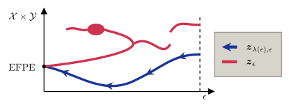
Figure 1: Examples of the “smooth” sequence of equilibria 𝒛λ(ϵ),ϵsubscript𝒛𝜆italic-ϵitalic-ϵ\boldsymbol{z}_{\lambda(\epsilon),\epsilon} of regularized-perturbed games (in blue) and the sequence of ϵitalic-ϵ\epsilon-EFPEs 𝒛ϵsubscript𝒛italic-ϵ\boldsymbol{z}_{\epsilon} in the definition of EFPE (in red).
Algorithm 1 Compute EFPE
1: function Compute-EFPE({(λk,ϵk)}k,β,ηsubscriptsubscript𝜆𝑘subscriptitalic-ϵ𝑘𝑘𝛽𝜂\{(\lambda_{k},\epsilon_{k})\}_{k\in\mathbb{N}},\beta,\eta)
2: {(λk,ϵk)}ksubscriptsubscript𝜆𝑘subscriptitalic-ϵ𝑘𝑘\{(\lambda_{k},\epsilon_{k})\}_{k\in\mathbb{N}}: As in the statement of Theorem 2. β>1𝛽1\beta>1: Phase growing rate. η>0𝜂0\eta>0: Learning rate.
3:      𝒛(0)superscript𝒛0absent\boldsymbol{z}^{(0)}\leftarrow any (𝒙,𝒚)𝒳×𝒴𝒙𝒚𝒳𝒴(\boldsymbol{x},\boldsymbol{y})\in\mathcal{X}\times\mathcal{Y}; k0𝑘0k\leftarrow 0; T0𝑇0T\leftarrow 0
4:      while not exceeding time limit do
5:          kk+1𝑘𝑘1k\leftarrow k+1
6:          Instantiate game 𝒢k𝒢(λk,ϵk)subscript𝒢𝑘𝒢subscript𝜆𝑘subscriptitalic-ϵ𝑘\mathcal{G}_{k}\coloneqq\mathcal{G}(\lambda_{k},\epsilon_{k})
7:          Tkβksubscript𝑇𝑘superscript𝛽𝑘T_{k}\leftarrow\beta^{k}; TT+Tk𝑇𝑇subscript𝑇𝑘T\leftarrow T+T_{k}
8:          𝒛Tk(k)subscriptsuperscript𝒛𝑘subscript𝑇𝑘absent\boldsymbol{z}^{(k)}_{T_{k}}\leftarrow Solve(𝒢k,Tk,𝒛Tk1(k1),η)subscript𝒢𝑘subscript𝑇𝑘subscriptsuperscript𝒛𝑘1subscript𝑇𝑘1𝜂(\mathcal{G}_{k},T_{k},\boldsymbol{z}^{(k-1)}_{T_{k-1}},\eta)      
9:      return 𝒛Tk(k)subscriptsuperscript𝒛𝑘subscript𝑇𝑘\boldsymbol{z}^{(k)}_{T_{k}}
Algorithm 2 Solve game 𝒢ksubscript𝒢𝑘\mathcal{G}_{k}
1: function Solve(𝒢k,Tk,𝒛1/2(k),ηsubscript𝒢𝑘subscript𝑇𝑘subscriptsuperscript𝒛𝑘12𝜂\mathcal{G}_{k},T_{k},\boldsymbol{z}^{(k)}_{-{1}/{2}},\eta)
2:      for t=0,,Tk1𝑡0subscript𝑇𝑘1t=0,\ldots,T_{k}-1 do
3:          𝒙t+12(k)argmax𝒙𝒳{𝒙𝑼𝒚t(k)1λkd1ϵk(𝒙)1ηD1ϵk(𝒙|𝒙t12(k))}subscriptsuperscript𝒙𝑘𝑡12subscript𝒙𝒳superscript𝒙top𝑼superscriptsubscript𝒚𝑡𝑘1subscript𝜆𝑘superscriptsubscript𝑑1subscriptitalic-ϵ𝑘𝒙1𝜂superscriptsubscript𝐷1subscriptitalic-ϵ𝑘conditional𝒙subscriptsuperscript𝒙𝑘𝑡12\boldsymbol{x}^{(k)}_{t+\frac{1}{2}}\leftarrow\arg\max\limits_{\boldsymbol{x}\in\mathcal{X}}\left\{\boldsymbol{x}^{\top}\boldsymbol{U}\boldsymbol{y}_{t}^{(k)}-\frac{1}{\lambda_{k}}{d_{1}^{\epsilon_{k}}(\boldsymbol{x})}-\frac{1}{\eta}D_{1}^{\epsilon_{k}}\left(\boldsymbol{x}|\boldsymbol{x}^{(k)}_{t-\frac{1}{2}}\right)\right\}
4:          𝒙t+1(k)argmax𝒙𝒳{𝒙𝑼𝒚t(k)1λkdϵk(𝒙)ηD1ϵk(𝒙|𝒙t+12(k))}subscriptsuperscript𝒙𝑘𝑡1subscript𝒙𝒳superscript𝒙top𝑼superscriptsubscript𝒚𝑡𝑘1subscript𝜆𝑘superscript𝑑subscriptitalic-ϵ𝑘𝒙𝜂superscriptsubscript𝐷1subscriptitalic-ϵ𝑘conditional𝒙subscriptsuperscript𝒙𝑘𝑡12\boldsymbol{x}^{(k)}_{t+1}\leftarrow\arg\max\limits_{\boldsymbol{x}\in\mathcal{X}}\left\{\boldsymbol{x}^{\top}\boldsymbol{U}\boldsymbol{y}_{t}^{(k)}-\frac{1}{\lambda_{k}}{d^{\epsilon_{k}}(\boldsymbol{x})}-{\eta}D_{1}^{\epsilon_{k}}\left(\boldsymbol{x}|\boldsymbol{x}^{(k)}_{t+\frac{1}{2}}\right)\right\}
5:          𝒚t+12(k)argmin𝒚𝒴{𝒙t(k),𝑼𝒚+1λkd2ϵk(𝒚)+1ηD2ϵk(𝒚|𝒚t12(k))}subscriptsuperscript𝒚𝑘𝑡12subscript𝒚𝒴subscriptsuperscript𝒙𝑘top𝑡𝑼𝒚1subscript𝜆𝑘superscriptsubscript𝑑2subscriptitalic-ϵ𝑘𝒚1𝜂superscriptsubscript𝐷2subscriptitalic-ϵ𝑘conditional𝒚subscriptsuperscript𝒚𝑘𝑡12\boldsymbol{y}^{(k)}_{t+\frac{1}{2}}\leftarrow\arg\min\limits_{\boldsymbol{y}\in\mathcal{Y}}\left\{\boldsymbol{x}^{(k),\top}_{t}\boldsymbol{U}\boldsymbol{y}+\frac{1}{\lambda_{k}}{d_{2}^{\epsilon_{k}}(\boldsymbol{y})}+\frac{1}{\eta}D_{2}^{\epsilon_{k}}\left(\boldsymbol{y}|\boldsymbol{y}^{(k)}_{t-\frac{1}{2}}\right)\right\}
6:          𝒚t+1(k)argmin𝒚𝒴{𝒙t(k),𝑼𝒚+1λkd2ϵk(𝒚)+1ηD2ϵk(𝒚|𝒚t+12(k))}subscriptsuperscript𝒚𝑘𝑡1subscript𝒚𝒴subscriptsuperscript𝒙𝑘top𝑡𝑼𝒚1subscript𝜆𝑘superscriptsubscript𝑑2subscriptitalic-ϵ𝑘𝒚1𝜂superscriptsubscript𝐷2subscriptitalic-ϵ𝑘conditional𝒚subscriptsuperscript𝒚𝑘𝑡12\boldsymbol{y}^{(k)}_{t+1}\leftarrow\arg\min\limits_{\boldsymbol{y}\in\mathcal{Y}}\left\{\boldsymbol{x}^{(k),\top}_{t}\boldsymbol{U}\boldsymbol{y}+\frac{1}{\lambda_{k}}d_{2}^{\epsilon_{k}}(\boldsymbol{y})+\frac{1}{\eta}D_{2}^{\epsilon_{k}}\left(\boldsymbol{y}|\boldsymbol{y}^{(k)}_{t+\frac{1}{2}}\right)\right\}      
7:      return 𝒛Tk(k)(𝒙Tk(k),𝒚Tk(k))subscriptsuperscript𝒛𝑘subscript𝑇𝑘superscriptsubscript𝒙subscript𝑇𝑘𝑘superscriptsubscript𝒚subscript𝑇𝑘𝑘\boldsymbol{z}^{(k)}_{{T_{k}}}\coloneqq\left(\boldsymbol{x}_{T_{k}}^{(k)},\boldsymbol{y}_{T_{k}}^{(k)}\right)

Moreover, using any sequence {(λk,ϵk)}ksubscriptsubscript𝜆𝑘subscriptitalic-ϵ𝑘𝑘\left\{(\lambda_{k},\epsilon_{k})\right\}_{k\in\mathbb{N}} such that λk+subscript𝜆𝑘\lambda_{k}\to+\infty and ϵk0subscriptitalic-ϵ𝑘0\epsilon_{k}\to 0 jointly as k+𝑘k\to+\infty does not always lead to EFPEs, as shown by the following proposition:

Proposition 1.

There exist EFGs for which

limλ[limϵ0𝒛λ,ϵ]limϵ0[limλ𝒛λ,ϵ],subscript𝜆delimited-[]subscriptitalic-ϵ0superscriptsubscript𝒛𝜆italic-ϵsubscriptitalic-ϵ0delimited-[]subscript𝜆superscriptsubscript𝒛𝜆italic-ϵ\lim\limits_{\lambda\to\infty}\left[\lim\limits_{\epsilon\to 0}\boldsymbol{z}_{\lambda,\epsilon}^{\star}\right]\neq\lim\limits_{\epsilon\to 0}\left[\lim\limits_{\lambda\to\infty}\boldsymbol{z}_{\lambda,\epsilon}^{\star}\right],

and limλ[limϵ0𝐳λ,ϵ]subscript𝜆delimited-[]subscriptitalic-ϵ0superscriptsubscript𝐳𝜆italic-ϵ\lim_{\lambda\to\infty}\left[\lim_{\epsilon\to 0}\boldsymbol{z}_{\lambda,\epsilon}^{\star}\right] is not an EFPE.

Then, by well-known results on iterated limits (Steinlage, 1971), we have that the double limit lim(λ,ϵ)(+,0)𝒛λ,ϵsubscript𝜆italic-ϵ0subscriptsuperscript𝒛𝜆italic-ϵ\lim_{(\lambda,\epsilon)\to(+\infty,0)}\boldsymbol{z}^{\star}_{\lambda,\epsilon} may not exist. This immediately implies that one cannot consider any arbitrary sequence {(λk,ϵk)}ksubscriptsubscript𝜆𝑘subscriptitalic-ϵ𝑘𝑘\left\{(\lambda_{k},\epsilon_{k})\right\}_{k\in\mathbb{N}} in order to define a sequence of equilibria leading to an EFPE. Indeed, the only guarantee that one gets is that the sequence leads to an NE of the original EFG. As a result, the sequence {(λk,ϵk)}ksubscriptsubscript𝜆𝑘subscriptitalic-ϵ𝑘𝑘\left\{(\lambda_{k},\epsilon_{k})\right\}_{k\in\mathbb{N}} must be built in a specific way.

Next, we show that we need sequences {(λk,ϵk)}ksubscriptsubscript𝜆𝑘subscriptitalic-ϵ𝑘𝑘\left\{(\lambda_{k},\epsilon_{k})\right\}_{k\in\mathbb{N}} that are defined so that the sequence made by the λksubscript𝜆𝑘\lambda_{k} converges faster than that of the ϵksubscriptitalic-ϵ𝑘\epsilon_{k}. Formally:

Theorem 2.

Given any EFG and a sequence {(λk,ϵk)}ksubscriptsubscript𝜆𝑘subscriptitalic-ϵ𝑘𝑘\left\{(\lambda_{k},\epsilon_{k})\right\}_{k\in\mathbb{N}} such that λk+subscript𝜆𝑘\lambda_{k}\to+\infty, ϵk0subscriptitalic-ϵ𝑘0\epsilon_{k}\to 0 as k+𝑘k\to+\infty and 1/λk<ϵkd1subscript𝜆𝑘superscriptsubscriptitalic-ϵ𝑘𝑑1/\lambda_{k}<\epsilon_{k}^{d} for a sufficiently large d𝑑d\in\mathbb{N}, limk+𝐳λk,ϵksubscript𝑘subscriptsuperscript𝐳subscript𝜆𝑘subscriptitalic-ϵ𝑘\lim_{k\to+\infty}\boldsymbol{z}^{\star}_{\lambda_{k},\epsilon_{k}} is an EFPE.

The proof of Theorem 2 is based on the core idea that, by choosing λk>1/ϵkdsubscript𝜆𝑘1superscriptsubscriptitalic-ϵ𝑘𝑑\lambda_{k}>1/\epsilon_{k}^{d}, the resulting sequence (1/λk,ϵk)1subscript𝜆𝑘subscriptitalic-ϵ𝑘(1/\lambda_{k},\epsilon_{k}) is “close” to the one defined by the iterated limit in Corollary 1, which is guaranteed to be an EFPE. Indeed, this amounts to showing that, for k𝑘k sufficiently large, the sequence (1/λk,ϵk)1subscript𝜆𝑘subscriptitalic-ϵ𝑘(1/\lambda_{k},\epsilon_{k}) is close to (0,ϵk)0subscriptitalic-ϵ𝑘(0,\epsilon_{k}), where the latter sequence converges to an EFPE by Corollary 1.

4.3 The Need of Regularization

Next, we argue why adding a regularization component is of paramount importance in our setting. Indeed, one could argue that it would be more natural to track the sequence of ϵitalic-ϵ\epsilon-EFPEs that appear in the definition of EFPE (Definition 1). However, such a methodology would not work. Indeed, such a natural sequence, tough always admitting a limit point, can have discontinuities, bifurcations, multiple branches, and other irregularities, which are drawback inherited by the convoluted structure of NE in linear games. In particular, non-uniqueness alone would doom any method that relies on last-iterate convergence, since uniqueness is a key assumption in such methods.

On the other hand, our sequence of equilibria defined in terms of regularized-perturbed games is 𝒞superscript𝒞\mathcal{C}^{\infty}-differentiable and it identifies a unique branch, while sharing the same limit point with the sequence in the definition of EFPE. This renders our sequence of equilibria much easier to track.

Figure 1 provides a depiction of the sequence used in the definition of EFPE and the one generated by our regularized-perturbed games.

5 Efficient Last-iterate Algorithm for EFPEs

We are now ready to introduce our last-iterate algorithm that converges to an (exact) EFPE (Algorithm 1). The algorithm works by tracking a sequence of equilibria 𝒛k𝒛λk,ϵksubscriptsuperscript𝒛𝑘subscriptsuperscript𝒛subscript𝜆𝑘subscriptitalic-ϵ𝑘\boldsymbol{z}^{\star}_{k}\coloneqq\boldsymbol{z}^{\star}_{\lambda_{k},\epsilon_{k}} of regularized-perturbed games 𝒢k𝒢(λk,ϵk)subscript𝒢𝑘𝒢subscript𝜆𝑘subscriptitalic-ϵ𝑘\mathcal{G}_{k}\coloneqq\mathcal{G}(\lambda_{k},\epsilon_{k}) by letting k+𝑘k\to+\infty, where the latter games are defined by means of a sequence {(λk,ϵk)}ksubscriptsubscript𝜆𝑘subscriptitalic-ϵ𝑘𝑘\left\{(\lambda_{k},\epsilon_{k})\right\}_{k\in\mathbb{N}} as in the statement of Theorem 2.

Algorithm 1 works in phases. For every k𝑘k\in\mathbb{N}, the k𝑘k-th phase of the algorithm is devoted to finding a suitable approximation of the equilibrium 𝒛ksubscriptsuperscript𝒛𝑘\boldsymbol{z}^{\star}_{k} of 𝒢ksubscript𝒢𝑘\mathcal{G}_{k}. This is achieved by performing Tkβksubscript𝑇𝑘superscript𝛽𝑘T_{k}\coloneqq\beta^{k} (for a given β>1𝛽1\beta>1) iterations of a last-iterate sub-procedure (Algorithm 2) that converges linearly to an approximate equilibrium of 𝒢ksubscript𝒢𝑘\mathcal{G}_{k} (see Theorem 3). We remark that, in any given phase k𝑘k, finding an approximation of 𝒛ksubscriptsuperscript𝒛𝑘\boldsymbol{z}^{\star}_{k} is sufficient, since the sequence made by the 𝒛ksuperscriptsubscript𝒛𝑘\boldsymbol{z}_{k}^{\star} has the only purpose of identifying EFPEs as its limit points.

Algorithm 2 is an extension of the OOMD algorithm, when instantiated for sequence-form strategy sets. Similarly to the OOMD algorithm, Algorithm 2 performs suitably-defined intermediate updates, labeled with the subscripts t+12𝑡12t+\frac{1}{2}. This enables the algorithm to converge last iterate.

Notice that, in our setting, it is not possible to use the standard update rule of OOMD, which would work by directly feeding the algorithm with the gradients of the utility functions fλk,ϵksubscript𝑓subscript𝜆𝑘subscriptitalic-ϵ𝑘f_{\lambda_{k},\epsilon_{k}} of regularized-perturbed games 𝒢ksubscript𝒢𝑘\mathcal{G}_{k}. This is because such functions are non-smooth due to the diϵksuperscriptsubscript𝑑𝑖subscriptitalic-ϵ𝑘d_{i}^{\epsilon_{k}} having unbounded gradient norm near the boundaries of 𝒳ϵk×𝒴ϵksuperscript𝒳subscriptitalic-ϵ𝑘superscript𝒴subscriptitalic-ϵ𝑘\mathcal{X}^{\epsilon_{k}}\times\mathcal{Y}^{\epsilon_{k}}. Indeed, diϵksuperscriptsubscript𝑑𝑖subscriptitalic-ϵ𝑘d_{i}^{\epsilon_{k}} are Legendre functions (Cesa-Bianchi and Lugosi, 2006). In order to circumvent this issue, we exploit an idea first introduced by the composite objective mirror descent algorithm (Duchi et al., 2010), which consists in avoiding the linearization of the non-smooth part in the utility function in order to get away with the non-Lipschitzness of the gradients. The following theorem formally states the last-iterate convergence guarantees of Algorithm 2.

Theorem 3.

Given η1/2𝐔2𝜂12subscriptnorm𝐔2\eta\leq{1}/{\sqrt{2}{\|\boldsymbol{U}\|_{2}}}, for every phase k𝑘k\in\mathbb{N} and round t{1,,Tk}𝑡1subscript𝑇𝑘t\in\{1,\ldots,T_{k}\}, Algorithm 2 guarantees that:

𝒛k𝒛t(k)22[2Dϵk(𝒛k|𝒛0(k))]1/2(λkλk+η)t/2,subscriptnormsuperscriptsubscript𝒛𝑘subscriptsuperscript𝒛𝑘𝑡22superscriptdelimited-[]2superscript𝐷subscriptitalic-ϵ𝑘conditionalsuperscriptsubscript𝒛𝑘subscriptsuperscript𝒛𝑘012superscriptsubscript𝜆𝑘subscript𝜆𝑘𝜂𝑡2\|\boldsymbol{z}_{k}^{\star}-\boldsymbol{z}^{(k)}_{t}\|_{2}\leq 2\left[2D^{\epsilon_{k}}\left(\boldsymbol{z}_{k}^{\star}|\boldsymbol{z}^{(k)}_{0}\right)\right]^{1/2}\left(\frac{\lambda_{k}}{\lambda_{k}+\eta}\right)^{t/2},

where Dϵk(𝐳|𝐳~):=D1ϵk(𝐱|𝐱~)+D2ϵk(𝐲|𝐲~)assignsuperscript𝐷subscriptitalic-ϵ𝑘conditional𝐳~𝐳subscriptsuperscript𝐷subscriptitalic-ϵ𝑘1conditional𝐱~𝐱subscriptsuperscript𝐷subscriptitalic-ϵ𝑘2conditional𝐲~𝐲D^{\epsilon_{k}}(\boldsymbol{z}|\tilde{\boldsymbol{z}}):=D^{\epsilon_{k}}_{1}(\boldsymbol{x}|\tilde{\boldsymbol{x}})+D^{\epsilon_{k}}_{2}(\boldsymbol{y}|\tilde{\boldsymbol{y}}).

We also remark that the technique we employ in the proof of the theorem above can be generalized to achieve last-iterate convergence to equilibria of EFGs for any dilated Legendre regularization functions disubscript𝑑𝑖d_{i}. Indeed, our results do not rely on the specific shape of the disubscript𝑑𝑖d_{i}, and the ones we used are specifically tailored only to get convergence to EFPEs.

5.1 Convergence Analysis

By exploiting the convergence analysis of Algorithm 2 (Theorem 3), the following theorem formally proves the convergence guarantees of Algorithm 1 to (exact) EFPEs.

Theorem 4.

Given any sequence {(λk,ϵk)}ksubscriptsubscript𝜆𝑘subscriptitalic-ϵ𝑘𝑘\{(\lambda_{k},\epsilon_{k})\}_{k\in\mathbb{N}} defined as in Theorem 2 satisfying ηλk2ηβk/2𝜂subscriptsuperscript𝜆2𝑘𝜂superscript𝛽𝑘2\eta\leq\lambda^{2}_{k}\leq\eta\beta^{k}/2 for every k𝑘k\in\mathbb{N}, Algorithm 1 grantees that limk𝐳Tk(k)subscript𝑘superscriptsubscript𝐳subscript𝑇𝑘𝑘\lim_{k\to\infty}\boldsymbol{z}_{T_{k}}^{(k)} is an EFPE.

Moreover, we can exploit the strongly convex-concave structure of the utility functions fλ,ϵsubscript𝑓𝜆italic-ϵf_{\lambda,\epsilon} to prove Nash gap guarantees for regularized-perturbed games 𝒢λ,ϵsubscript𝒢𝜆italic-ϵ\mathcal{G}_{\lambda,\epsilon}, which can then be combined with Theorem 1 to obtain guarantees on the exploitability of 𝒛Tk(k)superscriptsubscript𝒛subscript𝑇𝑘𝑘\boldsymbol{z}_{T_{k}}^{(k)} in the original EFG. Formally:

Theorem 5.

Let 𝐳~(𝐱~,𝐲~)𝒳×𝒴~𝐳~𝐱~𝐲𝒳𝒴\tilde{\boldsymbol{z}}\coloneqq(\tilde{\boldsymbol{x}},\tilde{\boldsymbol{y}})\in\mathcal{X}\times\mathcal{Y} be such that it holds 𝐳λ,ϵ𝐳~2νsubscriptnormsubscriptsuperscript𝐳𝜆italic-ϵ~𝐳2𝜈\|\boldsymbol{z}^{\star}_{\lambda,\epsilon}-\tilde{\boldsymbol{z}}\|_{2}\leq\nu for some ν>0𝜈0\nu>0, then we have:

Gap(𝒙~,𝒚~)ν|Σ|3/2+8C/λ,𝐺𝑎𝑝~𝒙~𝒚𝜈superscriptΣ328𝐶𝜆Gap(\tilde{\boldsymbol{x}},\tilde{\boldsymbol{y}})\leq\nu|\Sigma|^{3/2}+{8C}/{\lambda},

where |Σ|max{|Σ1|,|Σ2|}ΣsubscriptΣ1subscriptΣ2|\Sigma|\coloneqq\max\{|\Sigma_{1}|,|\Sigma_{2}|\} and C>0𝐶0C>0 is a constant that depends polynomially in maxi{1,2}|i|subscript𝑖12subscript𝑖\max_{i\in\{1,2\}}|\mathcal{I}_{i}|, maxI12αIsubscript𝐼subscript1subscript2subscript𝛼𝐼\max_{I\in\mathcal{I}_{1}\cup\mathcal{I}_{2}}\alpha_{I}, and maxI12lognIsubscript𝐼subscript1subscript2subscript𝑛𝐼\max_{I\in\mathcal{I}_{1}\cup\mathcal{I}_{2}}\log n_{I}.

As a direct corollary, we can prove the following guarantees in terms of Nash gap for Algorithm 1.

Corollary 2.

Given any sequence {(λk,ϵk)}ksubscriptsubscript𝜆𝑘subscriptitalic-ϵ𝑘𝑘\{(\lambda_{k},\epsilon_{k})\}_{k\in\mathbb{N}} as in Theorem 4, at the end of every phase k𝑘k\in\mathbb{N} of Algorithm 1:

Gap(𝒙Tk(k),𝒚Tk(k))4λk|Σ|32[2Dϵk(𝒛k|𝒛0(k))]12+8Cλk,𝐺𝑎𝑝subscriptsuperscript𝒙𝑘subscript𝑇𝑘subscriptsuperscript𝒚𝑘subscript𝑇𝑘4subscript𝜆𝑘superscriptΣ32superscriptdelimited-[]2superscript𝐷subscriptitalic-ϵ𝑘conditionalsuperscriptsubscript𝒛𝑘superscriptsubscript𝒛0𝑘128𝐶subscript𝜆𝑘Gap\left(\boldsymbol{x}^{(k)}_{T_{k}},\boldsymbol{y}^{(k)}_{T_{k}}\right)\leq\frac{4}{\lambda_{k}}|\Sigma|^{\frac{3}{2}}\left[2D^{\epsilon_{k}}(\boldsymbol{z}_{k}^{\star}|\boldsymbol{z}_{0}^{(k)})\right]^{\frac{1}{2}}+\frac{8C}{\lambda_{k}},

where ΣΣ\Sigma and C𝐶C are as in Theorem 4.

The result above justifies the need of the exponential growth of the number of rounds Tksubscript𝑇𝑘T_{k}. Indeed, it shows that, after T=j=1kβj=O(βk)𝑇superscriptsubscript𝑗1𝑘superscript𝛽𝑗𝑂superscript𝛽𝑘T=\sum_{j=1}^{k}\beta^{j}=O(\beta^{k}) rounds, one gets a Nash gap of the order of O(1/λk)𝑂1subscript𝜆𝑘O(1/\lambda_{k}). Thus, by choosing λk=O(βk/2)subscript𝜆𝑘𝑂superscript𝛽𝑘2\lambda_{k}=O(\beta^{k/2}) (which is the largest order of λksubscript𝜆𝑘\lambda_{k} allowed by Corollary 2), we have a bound of O(1/T)𝑂1𝑇O(1/\sqrt{T}) on the Nash gap.

Notice that Theorem 2 shows asymptotic convergence in terms of 2subscript2\ell_{2}-distance to an EFPE, while Corollary 2 shows convergence in terms of Nash gap. Determining whether it is possible to show finite convergence rates also for the 2subscript2\ell_{2}-distance to the set of EFPEs requires additional research. The difficulty of such an inquiry is that, even in (non-perturbed) normal-form games, our problem reduces to the one of finding convergence rates to limit-quantal equilibria, which is still an open problem.

5.2 Efficient Decomposition

The pseudo-code formulation of Algorithm 2 does not allow it to scale efficiently, since at each iteration it requires the solution of four convex optimization problems defined over the whole sequence-form strategy set 𝒳𝒳\mathcal{X} or 𝒴𝒴\mathcal{Y}.

Next, we show that each iteration of Algorithm 2 can indeed be implemented efficiently by directly working on the game tree. In particular, we show how to implement each update in Algorithm 2 so that: (i) it is performed recursively by means of a bottom-up visit of one player’s infosets; and (ii) at every visited infoset, it only requires the application of a local update that is done by applying a closed-form formula.

In order to do that, we exploit a technique that has been originally introduced in (Hoda et al., 2010; Farina, Kroer, and Sandholm, 2021; Lee, Kroer, and Luo, 2021). By focusing on the first player (analogous facts hold for the second player), we have that if the following two facts hold:

  1. 1.

    the update rule can be expressed as a proximal gradient update, i.e., as the problem of computing the conjugate gradient d1ϵ,(𝒈~)argmax𝒙𝒳{𝒙𝒈~d1ϵ(𝒙)}superscriptsubscript𝑑1italic-ϵ~𝒈subscript𝒙𝒳superscript𝒙top~𝒈superscriptsubscript𝑑1italic-ϵ𝒙\nabla d_{1}^{\epsilon,*}(\tilde{\boldsymbol{g}})\coloneqq\arg\max_{\boldsymbol{x}\in\mathcal{X}}\left\{\boldsymbol{x}^{\top}\tilde{\boldsymbol{g}}-d_{1}^{\epsilon}(\boldsymbol{x})\right\} of the dilated function d1ϵsuperscriptsubscript𝑑1italic-ϵd_{1}^{\epsilon} for some 𝒈~|Σ1|~𝒈superscriptsubscriptΣ1\tilde{\boldsymbol{g}}\in\mathbb{R}^{|\Sigma_{1}|}, and

  2. 2.

    for all I1𝐼subscript1I\in\mathcal{I}_{1} and 𝒈~nI~𝒈superscriptsubscript𝑛𝐼\tilde{\boldsymbol{g}}\in\mathbb{R}^{n_{I}}, the local conjugate gradient dΔIϵ,(𝒈~)argmax𝒘ΔI{𝒘𝒈~d1ϵ(𝒘)}superscriptsubscript𝑑subscriptΔ𝐼italic-ϵ~𝒈subscript𝒘subscriptΔ𝐼superscript𝒘top~𝒈superscriptsubscript𝑑1italic-ϵ𝒘\nabla d_{\Delta_{I}}^{\epsilon,*}(\tilde{\boldsymbol{g}})\coloneqq\arg\max_{\boldsymbol{w}\in\Delta_{I}}\left\{\boldsymbol{w}^{\top}\tilde{\boldsymbol{g}}-d_{1}^{\epsilon}(\boldsymbol{w})\right\} and the local gradient dΔIϵ(𝒈~)superscriptsubscript𝑑subscriptΔ𝐼italic-ϵ~𝒈\nabla d_{\Delta_{I}}^{\epsilon}(\tilde{\boldsymbol{g}}) have a closed-form solution,

then the overall updated can be computed efficiently in terms of requirements (i) and (ii) described above.

However, Algorithm 2 employs update rules that, a priori, are differently to those studied in (Hoda et al., 2010) and its follow ups. Thankfully, the following theorem show that the approach described above can still be employed on the update rules of Algorithm 2. Formally:

Theorem 6.

(i) The updates of Algorithm 2 of the form

argmax𝒙𝒳{𝒙𝒈d1ϵ(𝒙)λ1ηD1ϵ(𝒙|𝒙~)}subscript𝒙𝒳superscript𝒙top𝒈superscriptsubscript𝑑1italic-ϵ𝒙𝜆1𝜂superscriptsubscript𝐷1italic-ϵconditional𝒙~𝒙\displaystyle\arg\max\limits_{\boldsymbol{x}\in\mathcal{X}}\left\{\boldsymbol{x}^{\top}\boldsymbol{g}-\frac{d_{1}^{\epsilon}(\boldsymbol{x})}{\lambda}-\frac{1}{\eta}D_{1}^{\epsilon}(\boldsymbol{x}|\tilde{\boldsymbol{x}})\right\}

for some vectors 𝐠,𝐱~|Σ1|𝐠~𝐱superscriptsubscriptΣ1\boldsymbol{g},\tilde{\boldsymbol{x}}\in\mathbb{R}^{|\Sigma_{1}|} and ϵ>0italic-ϵ0\epsilon>0 can be formulated as the computation of the conjugate gradient d1ϵ,(𝐠~)superscriptsubscript𝑑1italic-ϵ~𝐠\nabla d_{1}^{\epsilon,*}(\tilde{\boldsymbol{g}}) for a suitably-defined, efficiently-computable vector 𝐠~|Σ1|~𝐠superscriptsubscriptΣ1\tilde{\boldsymbol{g}}\in\mathbb{R}^{|\Sigma_{1}|}.

(ii) For every ϵ>0ϵ0\epsilon>0, I1Isubscript1I\in\mathcal{I}_{1}, and 𝐠~nI~𝐠superscriptsubscriptnI\tilde{\boldsymbol{g}}\in\mathbb{R}^{n_{I}}, it holds:

dΔIϵ,(𝒈~)[a]=(1ϵnI)e𝒈~[a]bA(I)e𝒈~[b]+ϵaA(I).formulae-sequencesuperscriptsubscript𝑑subscriptΔ𝐼italic-ϵ~𝒈delimited-[]𝑎1italic-ϵsubscript𝑛𝐼superscript𝑒~𝒈delimited-[]𝑎subscript𝑏𝐴𝐼superscript𝑒~𝒈delimited-[]𝑏italic-ϵfor-all𝑎𝐴𝐼\nabla d_{\Delta_{I}}^{\epsilon,*}(\tilde{\boldsymbol{g}})[a]=(1-\epsilon\,n_{I})\frac{e^{\tilde{\boldsymbol{g}}[a]}}{\sum_{b\in A(I)}e^{\tilde{\boldsymbol{g}}[b]}}+\epsilon\quad\forall a\in A(I).

Moreover, the local gradient dΔIϵ(𝐠~)superscriptsubscript𝑑subscriptΔ𝐼italic-ϵ~𝐠\nabla d_{\Delta_{I}}^{\epsilon}(\tilde{\boldsymbol{g}}) can be computed as dΔIϵ(𝐠~)[a]=1+log(𝐠~[a]ϵ)superscriptsubscript𝑑subscriptΔ𝐼italic-ϵ~𝐠delimited-[]𝑎1~𝐠delimited-[]𝑎italic-ϵ\nabla d_{\Delta_{I}}^{\epsilon}(\tilde{\boldsymbol{g}})[a]=1+\log(\tilde{\boldsymbol{g}}[a]-\epsilon) for all aA(I)𝑎𝐴𝐼a\in A(I).

6 Experimental Evaluation

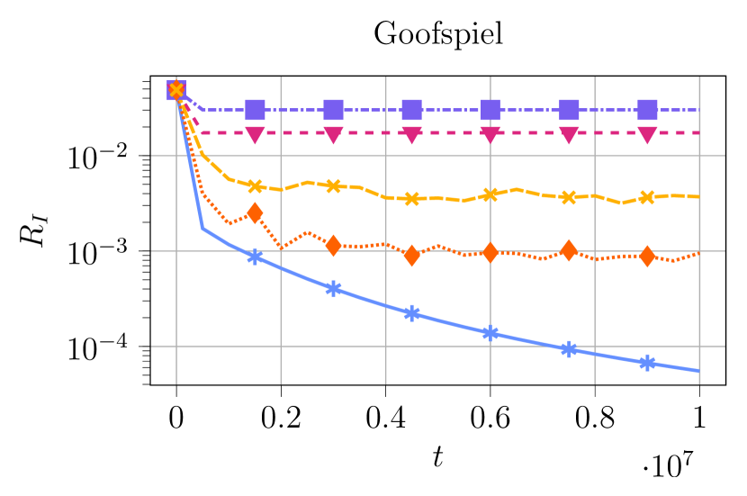
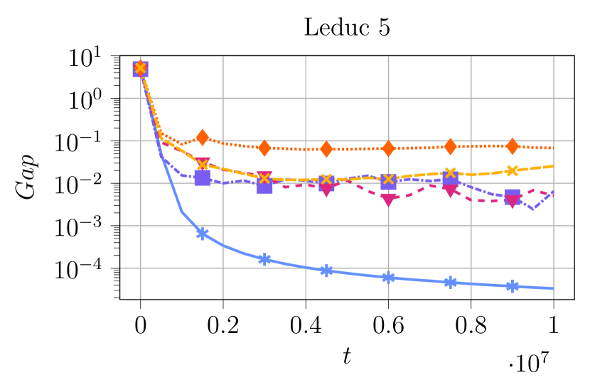
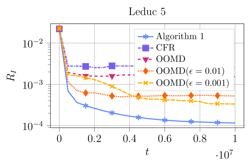
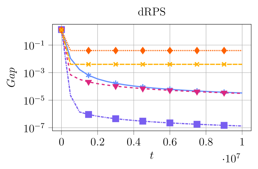
We conclude the paper by experimentally evaluating our algorithm (Algorithm 1) on a standard testbed of EFGs. In particular, we consider two simplified versions of Poker, called Kuhn (Kuhn, 1950) and Leduc (Southey et al., 2005), and a two-player card game called Goofspiel Ross (1971).444See Appendix C for a description of the games.

We evaluate our algorithm in terms of two metrics. The first one is the Nash gap, which is the standard metric employed to evaluate NE approximation. The second metric is the average infoset regret, called RIsubscript𝑅𝐼R_{I} for short. Given a pair of players’ strategies, this is defined as the average of the regrets that such strategies incur at all the infosets of the game. Specifically, the regret at an infoset is computed by assuming that such infoset is reached with probability one and by applying the Bayes’ rule to get a distribution encoding the probability of reaching each node in the infoset. Then, the regret is defined as the increase in utility from best-responding at that infoset and at all the subsequent ones.

We compare Algorithm 1 with two baseline algorithms for computing NEs, namely the CFR algorithm (Zinkevich et al., 2007) and the OOMD algorithm instantiated for EFG strategy spaces, as in Farina, Kroer, and Sandholm (2019). We run Algorithm 1 with β=1.001𝛽1.001\beta=1.001, η=2𝜂2\eta=2, ϵk=0.9999ksubscriptitalic-ϵ𝑘superscript0.9999𝑘\epsilon_{k}=0.9999^{k}, and λk=1/ϵk2subscript𝜆𝑘1superscriptsubscriptitalic-ϵ𝑘2\lambda_{k}=1/\epsilon_{k}^{2}. Moreover, we also compare the performances of Algorithm 1 with those obtained by the same algorithm while keeping the value of ϵitalic-ϵ\epsilon unchanged across its execution and eliminating regularization (i.e., 1/λ=01𝜆01/\lambda=0). In particular, we test ϵ=0.01italic-ϵ0.01\epsilon=0.01 and ϵ=0.001italic-ϵ0.001\epsilon=0.001. Since these baselines can also be viewed as the OOMD algorithm obtained by dilation of regularizer dΔIϵsuperscriptsubscript𝑑subscriptΔ𝐼italic-ϵd_{\Delta_{I}}^{\epsilon}, we name them OOMD(ϵitalic-ϵ\epsilon).

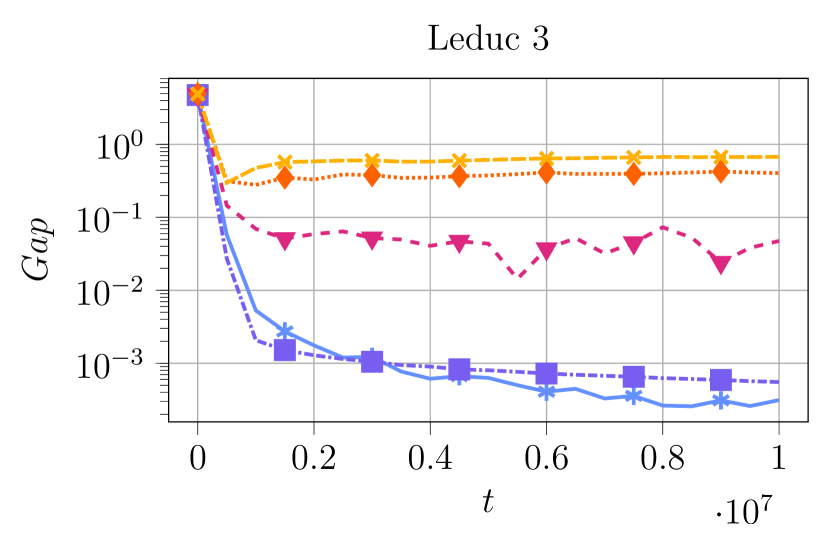
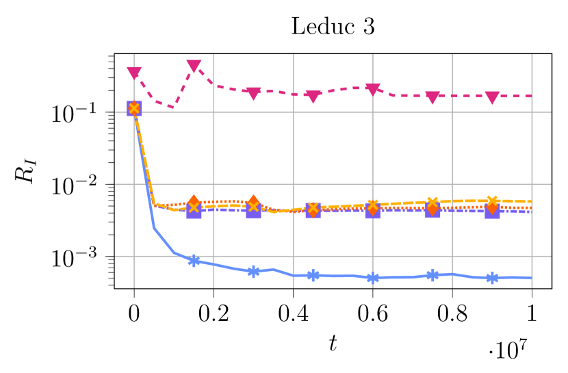
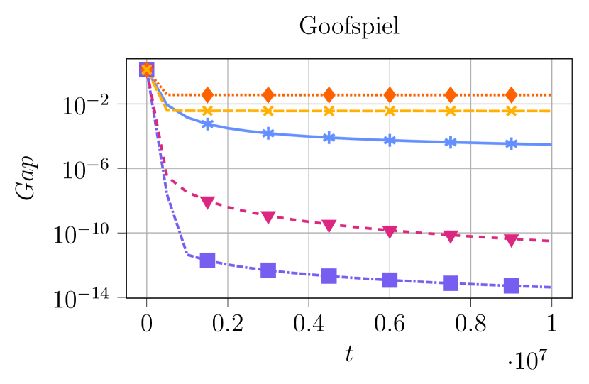
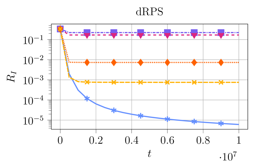
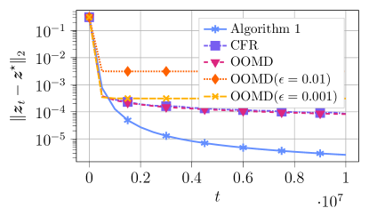
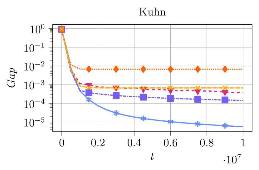
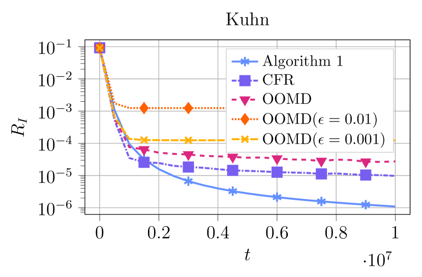
Figure 2 shows some results of our experimental evaluation (additional ones are in Appendix C).555For Algorithm 1, OOMD and OOMD(ϵ)italic-ϵ(\epsilon) we considered the last-iterates, while for CFR we considered the time average. As it is clear from the plots, Algorithm 1 outperforms of orders of magnitude the others in terms of average infoset regret. This was expected, since our algorithm is specifically tailored for converging to an EFPE, while the others only guarantee convergence to an NE or only find ϵitalic-ϵ\epsilon-EFPEs. Notice that Algorithm 1 also out-competes its variations that keep the value of ϵitalic-ϵ\epsilon unchanged, showing the importance of tuning regularization and perturbation terms jointly in order to converge to exact EFPEs. Indeed, every method that finds approximate equilibria of the perturbed game provably fails in getting both zero Nash gap and zero average infoset regret.

In terms of Nash gap, Algorithm 1 beats the baselines in Kuhn, it is (almost) matched by the CFR algorithm in Leduc, while it is outperformed by both the CFR and OOMD algorithms in Goofspiel. This is not surprising, since such algorithms are designed with the only (easier) objective of converging to an NE, and, thus, they perform better than Algorithm 1 in doing so on certain games. Indeed, the fact that Algorithm 1 is able to compete or even beat both the CFR and the OOMD algorithms on some game instances (see Kuhn and Leduc) was unexpected. This shows that the techniques that we employ not only do converge last-iterate to EFPEs but in also have the potential of leading to the design of algorithms that are superior to current state-of-the-art equilibrium-computation algorithms.
Refer to caption
Refer to caption
Refer to caption
Refer to caption
Refer to caption
Refer to caption
Figure 2: Results of the experimental evaluation. Algorithm 1 is compared with the baselines in terms of Nash gap (Left) and average infoset regret (Right).

References

  • Brown and Sandholm [2018] Brown, N.; and Sandholm, T. 2018. Superhuman AI for heads-up no-limit poker: Libratus beats top professionals. Science, 359(6374): 418–424.
  • Brown and Sandholm [2019] Brown, N.; and Sandholm, T. 2019. Superhuman AI for multiplayer poker. Science, 365(6456): 885–890.
  • Cesa-Bianchi and Lugosi [2006] Cesa-Bianchi, N.; and Lugosi, G. 2006. Prediction, learning, and games. Cambridge university press.
  • Duchi et al. [2010] Duchi, J. C.; Shalev-Shwartz, S.; Singer, Y.; and Tewari, A. 2010. Composite objective mirror descent. In COLT, volume 10, 14–26. Citeseer.
  • Farina and Gatti [2017] Farina, G.; and Gatti, N. 2017. Extensive-form perfect equilibrium computation in two-player games. In AAAI Conference on Artificial Intelligence, 502–508.
  • Farina, Gatti, and Sandholm [2018] Farina, G.; Gatti, N.; and Sandholm, T. 2018. Practical exact algorithm for trembling-hand equilibrium refinements in games. In Advances in Neural Information Processing Systems, 5039–5049.
  • Farina, Kroer, and Sandholm [2017] Farina, G.; Kroer, C.; and Sandholm, T. 2017. Regret minimization in behaviorally-constrained zero-sum games. In International Conference on Machine Learning, 1107–1116.
  • Farina, Kroer, and Sandholm [2019] Farina, G.; Kroer, C.; and Sandholm, T. 2019. Optimistic regret minimization for extensive-form games via dilated distance-generating functions. Advances in neural information processing systems, 32.
  • Farina, Kroer, and Sandholm [2021] Farina, G.; Kroer, C.; and Sandholm, T. 2021. Better regularization for sequential decision spaces: Fast convergence rates for Nash, correlated, and team equilibria. arXiv preprint arXiv:2105.12954.
  • Farina and Sandholm [2021] Farina, G.; and Sandholm, T. 2021. Equilibrium Refinement for the Age of Machines: The One-Sided Quasi-Perfect Equilibrium. Advances in Neural Information Processing Systems, 34: 8845–8856.
  • Gatti, Gilli, and Marchesi [2020] Gatti, N.; Gilli, M.; and Marchesi, A. 2020. A characterization of quasi-perfect equilibria. Games and Economic Behavior, 122: 240–255.
  • Hansen, Miltersen, and Sørensen [2010] Hansen, K. A.; Miltersen, P. B.; and Sørensen, T. B. 2010. The computational complexity of trembling hand perfection and other equilibrium refinements. In International Symposium on Algorithmic Game Theory, 198–209. Springer.
  • Hoda et al. [2010] Hoda, S.; Gilpin, A.; Pena, J.; and Sandholm, T. 2010. Smoothing techniques for computing Nash equilibria of sequential games. Mathematics of Operations Research, 35(2): 494–512.
  • Kroer, Farina, and Sandholm [2017] Kroer, C.; Farina, G.; and Sandholm, T. 2017. Smoothing Method for Approximate Extensive-Form Perfect Equilibrium. In International Joint Conference on Artificial Intelligence, 295–301.
  • Kuhn [1950] Kuhn, H. 1950. Simplified two-person poker. Contributions to the Theory of Games, 97–103.
  • Lee, Kroer, and Luo [2021] Lee, C.-W.; Kroer, C.; and Luo, H. 2021. Last-iterate convergence in extensive-form games. Advances in Neural Information Processing Systems, 34: 14293–14305.
  • McKelvey and Palfrey [1995] McKelvey, R. D.; and Palfrey, T. R. 1995. Quantal response equilibria for normal form games. Games and economic behavior, 10(1): 6–38.
  • Miltersen and Sørensen [2010] Miltersen, P. B.; and Sørensen, T. B. 2010. Computing a quasi-perfect equilibrium of a two-player game. Economic Theory, 42(1): 175–192.
  • Nash [1951] Nash, J. 1951. Non-cooperative games. Annals of mathematics, 286–295.
  • Rakhlin and Sridharan [2013] Rakhlin, S.; and Sridharan, K. 2013. Optimization, learning, and games with predictable sequences. Advances in Neural Information Processing Systems, 26.
  • Ross [1971] Ross, S. M. 1971. Goofspiel: The Game of Pure Strategy. Journal of Applied Probability, 8(3): 621–625.
  • Selten [1975] Selten, R. 1975. Reexamination of the perfectness concept for equilibrium points in extensive games. International journal of game theory, 4(1): 25–55.
  • Silver et al. [2016] Silver, D.; Huang, A.; Maddison, C. J.; Guez, A.; Sifre, L.; van den Driessche, G.; Schrittwieser, J.; Antonoglou, I.; Panneershelvam, V.; Lanctot, M.; Dieleman, S.; Grewe, D.; Nham, J.; Kalchbrenner, N.; Sutskever, I.; Lillicrap, T.; Leach, M.; Kavukcuoglu, K.; Graepel, T.; and Hassabis, D. 2016. Mastering the game of Go with deep neural networks and tree search. Nature, 529(7587): 484–489.
  • Southey et al. [2005] Southey, F.; Bowling, M.; Larson, B.; Piccione, C.; Burch, N.; Billings, D.; and Rayner, C. 2005. Bayes’ bluff: opponent modelling in poker. In Proceedings of the Twenty-First Conference on Uncertainty in Artificial Intelligence, 550–558.
  • Steinlage [1971] Steinlage, R. 1971. Nearly uniform convergence and interchange of limits. Publications de l’Institut Mathématique, 26(12): 115–129.
  • Van Damme [1991] Van Damme, E. 1991. Stability and perfection of Nash equilibria, volume 339. Springer.
  • Von Stengel [1996] Von Stengel, B. 1996. Efficient computation of behavior strategies. Games and Economic Behavior, 14(2): 220–246.
  • Wei et al. [2020] Wei, C.-Y.; Lee, C.-W.; Zhang, M.; and Luo, H. 2020. Linear Last-iterate Convergence in Constrained Saddle-point Optimization. In International Conference on Learning Representations.
  • Zinkevich et al. [2007] Zinkevich, M.; Johanson, M.; Bowling, M.; and Piccione, C. 2007. Regret minimization in games with incomplete information. Advances in neural information processing systems, 20.

Appendix Index

The appendix is structured as follows:

  • Appendix A presents the proofs omitted from Section 4.

  • Appendix B provides the proofs and additional details omitted from Section 5 in the construction of Algorithm 1.

  • Appendix C provides additional experiments details and results.

Appendix A Proofs omitted from Section 4

Lemma 1.

For every I12𝐼subscript1subscript2I\in\mathcal{I}_{1}\cup\mathcal{I}_{2} and ϵ>0italic-ϵ0\epsilon>0, the function dΔIϵsuperscriptsubscript𝑑subscriptΔ𝐼italic-ϵd_{\Delta_{I}}^{\epsilon} is 111-strongly convex with respect to the Euclidean norm.

Proof.

For every 𝒘ΔI𝒘subscriptΔ𝐼\boldsymbol{w}\in\Delta_{I}, we have that:

2dΔIϵ(𝒘)𝒘[i]𝒘[j]={1𝒘[i]ϵifi=j0otherwise.superscript2superscriptsubscript𝑑subscriptΔ𝐼italic-ϵ𝒘𝒘delimited-[]𝑖𝒘delimited-[]𝑗cases1𝒘delimited-[]𝑖italic-ϵif𝑖𝑗0otherwise\frac{\partial^{2}d_{\Delta_{I}}^{\epsilon}(\boldsymbol{w})}{\partial\boldsymbol{w}[i]\partial\boldsymbol{w}[j]}=\begin{cases}\frac{1}{\boldsymbol{w}[i]-\epsilon}&\text{if}\quad i=j\\ 0&\text{otherwise}\end{cases}.

Thus, 2dΔIϵ(𝒘)𝑰nIsuperscript2superscriptsubscript𝑑subscriptΔ𝐼italic-ϵ𝒘subscript𝑰subscript𝑛𝐼\nabla^{2}d_{\Delta_{I}}^{\epsilon}(\boldsymbol{w})\geq\,\boldsymbol{I}_{n_{I}}, where 𝑰nsubscript𝑰𝑛\boldsymbol{I}_{n} denotes the n𝑛n-dimensional identity matrix. This completes the proof. ∎

Lemma 2.

For any ϵ>0italic-ϵ0\epsilon>0, the functions d1ϵsuperscriptsubscript𝑑1italic-ϵd_{1}^{\epsilon} and d2ϵsuperscriptsubscript𝑑2italic-ϵd_{2}^{\epsilon} are 111-strongly convex with respect to the Euclidean norm.

Proof.

This follows from Lemma 1, the expression of the weights αIsubscript𝛼𝐼\alpha_{I} in dΔIϵsuperscriptsubscript𝑑subscriptΔ𝐼italic-ϵd_{\Delta_{I}}^{\epsilon} in the definitions of d1ϵ()superscriptsubscript𝑑1italic-ϵd_{1}^{\epsilon}(\cdot) and d2ϵ()superscriptsubscript𝑑2italic-ϵd_{2}^{\epsilon}(\cdot), and by using Farina, Kroer, and Sandholm [2019, Corollary 1]. ∎

Lemma 3.

We have that |d1ϵ(𝐱)|Csuperscriptsubscript𝑑1italic-ϵ𝐱𝐶|d_{1}^{\epsilon}(\boldsymbol{x})|\leq C and |d2ϵ(𝐲)|Csuperscriptsubscript𝑑2italic-ϵ𝐲𝐶|d_{2}^{\epsilon}(\boldsymbol{y})|\leq C for all 𝐱,𝐲𝒳×𝒴𝐱𝐲𝒳𝒴\boldsymbol{x},\boldsymbol{y}\in\mathcal{X}\times\mathcal{Y} and any ϵminI1212nIitalic-ϵsubscript𝐼subscript1subscript212subscript𝑛𝐼\epsilon\leq\min\limits_{I\in\mathcal{I}_{1}\cup\mathcal{I}_{2}}\frac{1}{2n_{I}}. Moreover C𝛂maxi{1,2}|Ii|maxI12log(2nI)𝐶subscriptnorm𝛂subscript𝑖12subscript𝐼𝑖subscript𝐼subscript1subscript22subscript𝑛𝐼C\leq\|\boldsymbol{\alpha}\|_{\infty}\cdot\max\limits_{i\in\{1,2\}}|I_{i}|\max\limits_{I\in\mathcal{I}_{1}\cup\mathcal{I}_{2}}\log(2n_{I}), where 𝛂|1|+|2|𝛂superscriptsubscript1subscript2\boldsymbol{\alpha}\in\mathbb{R}^{|\mathcal{I}_{1}|+|\mathcal{I}_{2}|} is a vector that contains all the components αIsubscript𝛼𝐼\alpha_{I} with I12𝐼subscript1subscript2I\in\mathcal{I}_{1}\cup\mathcal{I}_{2}.

Proof.

Consider the following inequalities:

max𝒙𝒳|d1ϵ(𝒙)|subscript𝒙𝒳superscriptsubscript𝑑1italic-ϵ𝒙\displaystyle\max\limits_{\boldsymbol{x}\in\mathcal{X}}|d_{1}^{\epsilon}(\boldsymbol{x})| I1αImax𝒘ΔI|dΔIϵ(𝒘)|absentsubscript𝐼subscript1subscript𝛼𝐼subscript𝒘subscriptΔ𝐼superscriptsubscript𝑑subscriptΔ𝐼italic-ϵ𝒘\displaystyle\leq\sum\limits_{I\in\mathcal{I}_{1}}{\alpha_{I}}\max\limits_{\boldsymbol{w}\in\Delta_{I}}|d_{\Delta_{I}}^{\epsilon}(\boldsymbol{w})|
I1αIlog(nI1ϵnI)absentsubscript𝐼subscript1subscript𝛼𝐼subscript𝑛𝐼1italic-ϵsubscript𝑛𝐼\displaystyle\leq\sum\limits_{I\in\mathcal{I}_{1}}\alpha_{I}\log\left(\frac{n_{I}}{1-\epsilon\cdot n_{I}}\right)
I1αIlog(2nI):=C𝒳,absentsubscript𝐼subscript1subscript𝛼𝐼2subscript𝑛𝐼assignsubscript𝐶𝒳\displaystyle\leq\sum\limits_{I\in\mathcal{I}_{1}}\alpha_{I}\log(2n_{I}):=C_{\mathcal{X}},

where we used that the maximum of dΔIϵ(𝒘)superscriptsubscript𝑑subscriptΔ𝐼italic-ϵ𝒘d_{\Delta_{I}}^{\epsilon}(\boldsymbol{w}) is attained in the center 𝒘[a]=1/nI𝒘delimited-[]𝑎1subscript𝑛𝐼\boldsymbol{w}[a]=1/n_{I}, for all aA(I)𝑎𝐴𝐼a\in A(I), and the last inequality follows from ϵminI1212nIitalic-ϵsubscript𝐼subscript1subscript212subscript𝑛𝐼\epsilon\leq\min\limits_{I\in\mathcal{I}_{1}\cup\mathcal{I}_{2}}\frac{1}{2n_{I}}. We can define C𝒴subscript𝐶𝒴C_{\mathcal{Y}} analogously for the second player and take C:=max{C𝒳,C𝒴}assign𝐶subscript𝐶𝒳subscript𝐶𝒴C:=\max\{C_{\mathcal{X}},C_{\mathcal{Y}}\}.

Then define the vector 𝜶𝜶\boldsymbol{\alpha} as the vector that contains the components αIsubscript𝛼𝐼\alpha_{I} for the first player and second player. Then, by Holder inequality, we have that C𝜶maxi{1,2}|Ii|maxI12log(2nI)𝐶subscriptnorm𝜶subscript𝑖12subscript𝐼𝑖subscript𝐼subscript1subscript22subscript𝑛𝐼C\leq\|\boldsymbol{\alpha}\|_{\infty}\cdot\max\limits_{i\in\{1,2\}}|I_{i}|\max\limits_{I\in\mathcal{I}_{1}\cup\mathcal{I}_{2}}\log(2n_{I}).

Lemma 4.

The following inequalities holds:

|max𝒙f(𝒙)max𝒚g(𝒚)|max𝒙|f(𝒙)g(𝒙)|subscript𝒙𝑓𝒙subscript𝒚𝑔𝒚subscript𝒙𝑓𝒙𝑔𝒙\displaystyle\left|\max\limits_{\boldsymbol{x}}f(\boldsymbol{x})-\max\limits_{\boldsymbol{y}}g(\boldsymbol{y})\right|\leq\max\limits_{\boldsymbol{x}}|f(\boldsymbol{x})-g(\boldsymbol{x})| (1)
|min𝒙f(𝒙)min𝒚g(𝒚)|max𝒙|f(𝒙)g(𝒙)|subscript𝒙𝑓𝒙subscript𝒚𝑔𝒚subscript𝒙𝑓𝒙𝑔𝒙\displaystyle\left|\min\limits_{\boldsymbol{x}}f(\boldsymbol{x})-\min\limits_{\boldsymbol{y}}g(\boldsymbol{y})\right|\leq\max\limits_{\boldsymbol{x}}|f(\boldsymbol{x})-g(\boldsymbol{x})| (2)
Proof.

Consider the following inequality:

f(𝒙)|f(𝒙)g(𝒙)|+g(𝒙)𝑓𝒙𝑓𝒙𝑔𝒙𝑔𝒙f(\boldsymbol{x})\leq|f(\boldsymbol{x})-g(\boldsymbol{x})|+g(\boldsymbol{x})

Applying the max\max operator to both sides of the previous equation and observing that max𝒙(|f(𝒙)g(𝒙)|+g(𝒙))max𝒙|f(𝒙)g(𝒙)|+max𝒙g(𝒙))\max\limits_{\boldsymbol{x}}(|f(\boldsymbol{x})-g(\boldsymbol{x})|+g(\boldsymbol{x}))\leq\max\limits_{\boldsymbol{x}}|f(\boldsymbol{x})-g(\boldsymbol{x})|+\max\limits_{\boldsymbol{x}}g(\boldsymbol{x})) we can rearrange the inequality to obtain:

max𝒙f(𝒙)max𝒙g(𝒙)max𝒙|f(𝒙)g(𝒙)|.subscript𝒙𝑓𝒙subscript𝒙𝑔𝒙subscript𝒙𝑓𝒙𝑔𝒙\max\limits_{\boldsymbol{x}}f(\boldsymbol{x})-\max\limits_{\boldsymbol{x}}g(\boldsymbol{x})\leq\max\limits_{\boldsymbol{x}}|f(\boldsymbol{x})-g(\boldsymbol{x})|.

We can in the same way obtain that:

max𝒙g(𝒙)max𝒙f(𝒙)max𝒙|f(𝒙)g(𝒙)|,subscript𝒙𝑔𝒙subscript𝒙𝑓𝒙subscript𝒙𝑓𝒙𝑔𝒙\max\limits_{\boldsymbol{x}}g(\boldsymbol{x})-\max\limits_{\boldsymbol{x}}f(\boldsymbol{x})\leq\max\limits_{\boldsymbol{x}}|f(\boldsymbol{x})-g(\boldsymbol{x})|,

which combined with the above let us conclude Equation (1). Now Equation (2) follows from considering Equation (1) with f(𝒙)𝑓𝒙-f(\boldsymbol{x}) instead of f(𝒙)𝑓𝒙f(\boldsymbol{x}) and g(𝒙)𝑔𝒙-g(\boldsymbol{x}) instead of g(𝒙)𝑔𝒙g(\boldsymbol{x}). ∎

See 1

Proof.

Let us consider the function f~ϵ:𝒳×𝒴:subscript~𝑓italic-ϵ𝒳𝒴\tilde{f}_{\epsilon}:\mathcal{X}\times\mathcal{Y}\to\mathbb{R} such that, for every 𝒙𝒳𝒙𝒳\boldsymbol{x}\in\mathcal{X} and 𝒚𝒴𝒚𝒴\boldsymbol{y}\in\mathcal{Y}, it holds:

f~ϵ(𝒙,𝒚)𝒙𝑼𝒚𝕀𝒳ϵ(𝒙)+𝕀𝒴ϵ(𝒚),subscript~𝑓italic-ϵ𝒙𝒚superscript𝒙top𝑼𝒚subscript𝕀superscript𝒳italic-ϵ𝒙subscript𝕀superscript𝒴italic-ϵ𝒚\tilde{f}_{\epsilon}(\boldsymbol{x},\boldsymbol{y})\coloneqq\boldsymbol{x}^{\top}\boldsymbol{U}\boldsymbol{y}-\mathbb{I}_{\mathcal{X}^{\epsilon}}(\boldsymbol{x})+\mathbb{I}_{\mathcal{Y}^{\epsilon}}(\boldsymbol{y}),

where 𝕀𝒲(𝒘)subscript𝕀𝒲𝒘\mathbb{I}_{\mathcal{W}}(\boldsymbol{w}) is 00 if 𝒘𝒲𝒘𝒲\boldsymbol{w}\in\mathcal{W}, while it is ++\infty if 𝒘𝒲𝒘𝒲\boldsymbol{w}\not\in\mathcal{W}.

First, it is easy to check that any (𝒙,𝒚)𝒳×𝒴𝒙𝒚𝒳𝒴(\boldsymbol{x},\boldsymbol{y})\in\mathcal{X}\times\mathcal{Y} such that f~ϵ(𝒙,𝒚)=max𝒙~𝒳min𝒚~𝒴f~ϵ(𝒙~,𝒚~)subscript~𝑓italic-ϵ𝒙𝒚subscript~𝒙𝒳subscript~𝒚𝒴subscript~𝑓italic-ϵ~𝒙~𝒚\tilde{f}_{\epsilon}(\boldsymbol{x},\boldsymbol{y})=\max_{\tilde{\boldsymbol{x}}\in\mathcal{X}}\min_{\tilde{\boldsymbol{y}}\in\mathcal{Y}}\tilde{f}_{\epsilon}(\tilde{\boldsymbol{x}},\tilde{\boldsymbol{y}}) is an ϵitalic-ϵ\epsilon-EFPE of the original EFG (see Definition 1).

Moreover, for any (𝒙,𝒚)𝒳ϵ×𝒴ϵ𝒙𝒚superscript𝒳italic-ϵsuperscript𝒴italic-ϵ(\boldsymbol{x},\boldsymbol{y})\in\mathcal{X}^{\epsilon}\times\mathcal{Y}^{\epsilon} it is easy to show that |fλ,ϵf~ϵ|=O(1/λ)subscript𝑓𝜆italic-ϵsubscript~𝑓italic-ϵ𝑂1𝜆|f_{\lambda,\epsilon}-\tilde{f}_{\epsilon}|=O(1/\lambda):

|fλ,ϵ(𝒙,𝒚)f~ϵ(𝒙,𝒚)|subscript𝑓𝜆italic-ϵ𝒙𝒚subscript~𝑓italic-ϵ𝒙𝒚\displaystyle|f_{\lambda,\epsilon}(\boldsymbol{x},\boldsymbol{y})-\tilde{f}_{\epsilon}(\boldsymbol{x},\boldsymbol{y})| |d1ϵ(𝒙)d2ϵ(𝒚)|λ2Cλ,absentsuperscriptsubscript𝑑1italic-ϵ𝒙superscriptsubscript𝑑2italic-ϵ𝒚𝜆2𝐶𝜆\displaystyle\leq\frac{\left|d_{1}^{\epsilon}(\boldsymbol{x})-d_{2}^{\epsilon}(\boldsymbol{y})\right|}{\lambda}\leq\frac{2C}{\lambda},

where C𝐶C is defined in Lemma 3.

Finally, let us consider the unique NE 𝒛λ,ϵ=(𝒙λ,ϵ,𝒚λ,ϵ)subscriptsuperscript𝒛𝜆italic-ϵsuperscriptsubscript𝒙𝜆italic-ϵsuperscriptsubscript𝒚𝜆italic-ϵ\boldsymbol{z}^{\star}_{\lambda,\epsilon}=(\boldsymbol{x}_{\lambda,\epsilon}^{\star},\boldsymbol{y}_{\lambda,\epsilon}^{\star}) of 𝒢(λ,ϵ)𝒢𝜆italic-ϵ\mathcal{G}(\lambda,\epsilon). By Lemma 4, we have that:

max𝒙𝒳ϵf~ϵ(𝒙,𝒚λ,ϵ)min𝒚𝒴ϵf~ϵ(𝒙λ,ϵ,𝒚)subscript𝒙superscript𝒳italic-ϵsubscript~𝑓italic-ϵ𝒙subscriptsuperscript𝒚𝜆italic-ϵsubscript𝒚superscript𝒴italic-ϵsubscript~𝑓italic-ϵsubscriptsuperscript𝒙𝜆italic-ϵ𝒚\displaystyle\max_{\boldsymbol{x}\in\mathcal{X}^{\epsilon}}\tilde{f}_{\epsilon}(\boldsymbol{x},\boldsymbol{y}^{\star}_{\lambda,\epsilon})-\min_{\boldsymbol{y}\in\mathcal{Y}^{\epsilon}}\tilde{f}_{\epsilon}(\boldsymbol{x}^{\star}_{\lambda,\epsilon},\boldsymbol{y}) |max𝒙𝒳ϵf~ϵ(𝒙,𝒚λ,ϵ)max𝒙𝒳ϵfλ,ϵ(𝒙,𝒚λ,ϵ)|+|min𝒚𝒴ϵf~ϵ(𝒙λ,ϵ,𝒚)min𝒚𝒴ϵfλ,ϵ(𝒙λ,ϵ,𝒚)|absentsubscript𝒙superscript𝒳italic-ϵsubscript~𝑓italic-ϵ𝒙subscriptsuperscript𝒚𝜆italic-ϵsubscript𝒙superscript𝒳italic-ϵsubscript𝑓𝜆italic-ϵ𝒙subscriptsuperscript𝒚𝜆italic-ϵsubscript𝒚superscript𝒴italic-ϵsubscript~𝑓italic-ϵsubscriptsuperscript𝒙𝜆italic-ϵ𝒚subscript𝒚superscript𝒴italic-ϵsubscript𝑓𝜆italic-ϵsubscriptsuperscript𝒙𝜆italic-ϵ𝒚\displaystyle\leq\left|\max_{\boldsymbol{x}\in\mathcal{X}^{\epsilon}}\tilde{f}_{\epsilon}(\boldsymbol{x},\boldsymbol{y}^{\star}_{\lambda,\epsilon})-\max_{\boldsymbol{x}\in\mathcal{X}^{\epsilon}}f_{\lambda,\epsilon}(\boldsymbol{x},\boldsymbol{y}^{\star}_{\lambda,\epsilon})\right|+\left|\min_{\boldsymbol{y}\in\mathcal{Y}^{\epsilon}}\tilde{f}_{\epsilon}(\boldsymbol{x}^{\star}_{\lambda,\epsilon},\boldsymbol{y})-\min_{\boldsymbol{y}\in\mathcal{Y}^{\epsilon}}f_{\lambda,\epsilon}(\boldsymbol{x}^{\star}_{\lambda,\epsilon},\boldsymbol{y})\right|
4Cλ,absent4𝐶𝜆\displaystyle\leq\frac{4C}{\lambda},

which concludes the proof. ∎

See 1

Proof.

Let us consider a game in which the two players play simultaneously and only once, having each of them three different actions available (i.e., a 3×3333\times 3 game in normal form). The following matrix encodes the first player’s payoffs for all the possible combinations of players’ actions:

[0.30.50.30.70.30.70.60.20.2]delimited-[]0.30.50.30.70.30.70.60.20.2\left[{\begin{array}[]{ccc}0.3&0.5&0.3\\ 0.7&0.3&0.7\\ 0.6&0.2&0.2\end{array}}\right]

By using the fact that any quantal equilibrium enjoys the "independence of irrelevant alternatives" property McKelvey and Palfrey [1995], we can prove that it holds:

limλ[limϵ0𝒛λ,ϵ]=([1/21/20],[1/62/31/6]),subscript𝜆delimited-[]subscriptitalic-ϵ0superscriptsubscript𝒛𝜆italic-ϵdelimited-[]12missing-subexpressionmissing-subexpression12missing-subexpressionmissing-subexpression0missing-subexpressionmissing-subexpressiondelimited-[]16missing-subexpressionmissing-subexpression23missing-subexpressionmissing-subexpression16missing-subexpressionmissing-subexpression\lim\limits_{\lambda\to\infty}\left[\lim\limits_{\epsilon\to 0}\boldsymbol{z}_{\lambda,\epsilon}^{\star}\right]=\left(\left[{\begin{array}[]{ccc}1/2\\ 1/2\\ 0\end{array}}\right],\left[{\begin{array}[]{ccc}1/6\\ 2/3\\ 1/6\end{array}}\right]\right),

where we expressed player’s strategies as the probability distributions that they induce over the three actions for ease of presentation. Moreover, the only EFPE of the game is:

𝒛=([1/21/20],[02/31/3]),superscript𝒛delimited-[]12missing-subexpressionmissing-subexpression12missing-subexpressionmissing-subexpression0missing-subexpressionmissing-subexpressiondelimited-[]0missing-subexpressionmissing-subexpression23missing-subexpressionmissing-subexpression13missing-subexpressionmissing-subexpression\boldsymbol{z}^{\star}=\left(\left[{\begin{array}[]{ccc}1/2\\ 1/2\\ 0\end{array}}\right],\left[{\begin{array}[]{ccc}0\\ 2/3\\ 1/3\end{array}}\right]\right),

since this is the unique NE that eliminates weakly dominated strategies, and, thus, it is an [Van Damme, 1991, Corollary 2.2.6]. This proves the proposition. ∎

See 2

Proof.

By Corollary 1, we have that

𝒛limϵ0[limλ𝒛λ,ϵ]superscript𝒛subscriptitalic-ϵ0delimited-[]subscript𝜆superscriptsubscript𝒛𝜆italic-ϵ\boldsymbol{z}^{\star}\coloneqq\lim\limits_{\epsilon\to 0}\left[\lim\limits_{\lambda\to\infty}\boldsymbol{z}_{\lambda,\epsilon}^{\star}\right]

is an EFPE. Let 𝒛ϵlimλ𝒛λ,ϵsuperscriptsubscript𝒛italic-ϵsubscript𝜆subscriptsuperscript𝒛𝜆italic-ϵ\boldsymbol{z}_{\epsilon}^{\star}\coloneqq\lim_{\lambda\to\infty}\boldsymbol{z}^{\star}_{\lambda,\epsilon} for all ϵ>0italic-ϵ0\epsilon>0. By definition of limit, for every τ>0𝜏0\tau>0 there exists Rϵ(τ)+subscript𝑅italic-ϵ𝜏subscriptR_{\epsilon}(\tau)\in\mathbb{R}_{+} such that |𝒛λ,ϵ𝒛ϵ|τsubscriptsuperscript𝒛𝜆italic-ϵsubscriptsuperscript𝒛italic-ϵ𝜏|\boldsymbol{z}^{\star}_{\lambda,\epsilon}-\boldsymbol{z}^{\star}_{\epsilon}|\leq\tau for all λ:λ>Rϵ(τ):𝜆𝜆subscript𝑅italic-ϵ𝜏\lambda\in\mathbb{R}:\lambda>R_{\epsilon}(\tau). Moreover, by looking at the outer limit in the definition of 𝒛superscript𝒛\boldsymbol{z}^{\star} we have that, for every τ>0superscript𝜏0\tau^{\prime}>0, there exists H(τ)+𝐻superscript𝜏subscriptH(\tau^{\prime})\in\mathbb{R}_{+} such that |𝒛ϵ𝒛|τsubscriptsuperscript𝒛italic-ϵsuperscript𝒛superscript𝜏|\boldsymbol{z}^{\star}_{\epsilon}-\boldsymbol{z}^{\star}|\leq\tau^{\prime} for all ϵ:|ϵ|H(τ):italic-ϵitalic-ϵ𝐻superscript𝜏\epsilon\in\mathbb{R}:|\epsilon|\leq H(\tau^{\prime}).

By using the triangular inequality, for every τ>0𝜏0\tau>0:

|𝒛ϵ,λ𝒛||𝒛ϵ,λ𝒛ϵ|+|𝒛ϵ𝒛|τsubscriptsuperscript𝒛italic-ϵ𝜆superscript𝒛subscriptsuperscript𝒛italic-ϵ𝜆subscriptsuperscript𝒛italic-ϵsubscriptsuperscript𝒛italic-ϵsuperscript𝒛𝜏\displaystyle|\boldsymbol{z}^{\star}_{\epsilon,\lambda}-\boldsymbol{z}^{\star}|\leq|\boldsymbol{z}^{\star}_{\epsilon,\lambda}-\boldsymbol{z}^{\star}_{\epsilon}|+|\boldsymbol{z}^{\star}_{\epsilon}-\boldsymbol{z}^{\star}|\leq\tau

for all λ:λ>Rϵ(τ/2):𝜆𝜆subscript𝑅italic-ϵ𝜏2\lambda\in\mathbb{R}:\lambda>R_{\epsilon}(\tau/2) and ϵ:|ϵ|H(τ/2):italic-ϵitalic-ϵ𝐻𝜏2\epsilon\in\mathbb{R}:|\epsilon|\leq H(\tau/2).

Moreover, if ϵkH(τ/2)subscriptitalic-ϵ𝑘𝐻𝜏2\epsilon_{k}\leq H(\tau/2), then λk>Rϵk(τ/2)subscript𝜆𝑘subscript𝑅subscriptitalic-ϵ𝑘𝜏2\lambda_{k}>R_{\epsilon_{k}}(\tau/2). This follows from the following inequalities:

λk>1ϵkd1H(τ/2)dRϵk(τ/2),subscript𝜆𝑘1superscriptsubscriptitalic-ϵ𝑘𝑑1𝐻superscript𝜏2𝑑subscript𝑅subscriptitalic-ϵ𝑘𝜏2\lambda_{k}>\frac{1}{\epsilon_{k}^{d}}\geq\frac{1}{H(\tau/2)^{d}}\geq R_{\epsilon_{k}}(\tau/2),

where the last inequality holds for any sufficiency large d𝑑d and the fact that Rϵk(τ/2)subscript𝑅subscriptitalic-ϵ𝑘𝜏2R_{\epsilon_{k}}(\tau/2) can be upper bounded for every k𝑘k (otherwise 𝒛0limλ𝒛λ,0superscriptsubscript𝒛0subscript𝜆subscriptsuperscript𝒛𝜆0\boldsymbol{z}_{0}^{\star}\coloneqq\lim_{\lambda\to\infty}\boldsymbol{z}^{\star}_{\lambda,0} would not exists).

As a result, for every τ>0𝜏0\tau>0 and for all k𝑘k\in\mathbb{N} such that ϵkH(τ/2)subscriptitalic-ϵ𝑘𝐻𝜏2\epsilon_{k}\leq H(\tau/2), it holds:

|𝒛ϵk,λk𝒛|τ,subscriptsuperscript𝒛subscriptitalic-ϵ𝑘subscript𝜆𝑘superscript𝒛𝜏\displaystyle|\boldsymbol{z}^{\star}_{\epsilon_{k},\lambda_{k}}-\boldsymbol{z}^{\star}|\leq\tau,

which concludes the proof. ∎

Appendix B Proofs omitted from Section 5

In this section is convenient to consider the join updates for the first and second player. If we define 𝒛=(𝒙,𝒚)𝒳×𝒴𝒛𝒙𝒚𝒳𝒴\boldsymbol{z}=(\boldsymbol{x},\boldsymbol{y})\in\mathcal{X}\times\mathcal{Y}, then it is easy to verify that updates of the form:

𝒙^=argmax𝒙𝒳{𝒙𝑼𝒚01λd1ϵ(𝒙)1ηD1ϵ(𝒙|𝒙~)}^𝒙subscript𝒙𝒳superscript𝒙top𝑼subscript𝒚01𝜆superscriptsubscript𝑑1italic-ϵ𝒙1𝜂superscriptsubscript𝐷1italic-ϵconditional𝒙~𝒙\displaystyle\hat{\boldsymbol{x}}=\arg\max\limits_{\boldsymbol{x}\in\mathcal{X}}\left\{\boldsymbol{x}^{\top}\boldsymbol{U}\boldsymbol{y}_{0}-\frac{1}{\lambda}d_{1}^{\epsilon}(\boldsymbol{x})-\frac{1}{\eta}D_{1}^{\epsilon}(\boldsymbol{x}|\tilde{\boldsymbol{x}})\right\} (3)
𝒚^=argmin𝒚𝒴{𝒙0𝑼𝒚+1λd2ϵ(𝒚)+1ηD2ϵ(𝒚|𝒚~)},^𝒚subscript𝒚𝒴superscriptsubscript𝒙0top𝑼𝒚1𝜆superscriptsubscript𝑑2italic-ϵ𝒚1𝜂superscriptsubscript𝐷2italic-ϵconditional𝒚~𝒚\displaystyle\hat{\boldsymbol{y}}=\arg\min\limits_{\boldsymbol{y}\in\mathcal{Y}}\left\{\boldsymbol{x}_{0}^{\top}\boldsymbol{U}\boldsymbol{y}+\frac{1}{\lambda}d_{2}^{\epsilon}(\boldsymbol{y})+\frac{1}{\eta}D_{2}^{\epsilon}(\boldsymbol{y}|\tilde{\boldsymbol{y}})\right\}, (4)

can be jointly expressed as:

𝒛^=argmin𝒛𝒳×𝒴{G(𝒛0)𝒛+1λHϵ(𝒛)+1ηDϵ(𝒛|𝒛~)},^𝒛subscript𝒛𝒳𝒴𝐺superscriptsubscript𝒛0top𝒛1𝜆superscript𝐻italic-ϵ𝒛1𝜂superscript𝐷italic-ϵconditional𝒛~𝒛\hat{\boldsymbol{z}}=\arg\min\limits_{\boldsymbol{z}\in\mathcal{X}\times\mathcal{Y}}\left\{G(\boldsymbol{z}_{0})^{\top}\boldsymbol{z}+\frac{1}{\lambda}H^{\epsilon}(\boldsymbol{z})+\frac{1}{\eta}D^{\epsilon}(\boldsymbol{z}|\tilde{\boldsymbol{z}})\right\},

where we define Hϵ(𝒛):=d1ϵ(𝒙)+d2ϵ(𝒚)assignsuperscript𝐻italic-ϵ𝒛subscriptsuperscript𝑑italic-ϵ1𝒙subscriptsuperscript𝑑italic-ϵ2𝒚H^{\epsilon}(\boldsymbol{z}):=d^{\epsilon}_{1}(\boldsymbol{x})+d^{\epsilon}_{2}(\boldsymbol{y}), Dϵ(𝒛|𝒛~):=D1ϵ(𝒙|𝒙~)+D2ϵ(𝒚|𝒚~)assignsuperscript𝐷italic-ϵconditional𝒛~𝒛superscriptsubscript𝐷1italic-ϵconditional𝒙~𝒙superscriptsubscript𝐷2italic-ϵconditional𝒚~𝒚D^{\epsilon}(\boldsymbol{z}|\tilde{\boldsymbol{z}}):=D_{1}^{\epsilon}(\boldsymbol{x}|\tilde{\boldsymbol{x}})+D_{2}^{\epsilon}(\boldsymbol{y}|\tilde{\boldsymbol{y}}) and G(𝒛):=(𝑼𝒚,𝑼𝒙)assign𝐺𝒛𝑼𝒚superscript𝑼top𝒙G(\boldsymbol{z}):=(-\boldsymbol{U}\boldsymbol{y},\boldsymbol{U}^{\top}\boldsymbol{x}).

B.1 Convergence Analysis

Lemma 5.

Let 𝐳λ,ϵsuperscriptsubscript𝐳𝜆italic-ϵ\boldsymbol{z}_{\lambda,\epsilon}^{\star} the unique NE of the game 𝒢λ,ϵsubscript𝒢𝜆italic-ϵ\mathcal{G}_{\lambda,\epsilon}, then for all 𝐳𝐳\boldsymbol{z}:

G(𝒛)(𝒛λ,ϵ𝒛)+1λ[Hϵ(𝒛λ,ϵ)Hϵ(𝒛)]0𝐺superscript𝒛topsuperscriptsubscript𝒛𝜆italic-ϵ𝒛1𝜆delimited-[]superscript𝐻italic-ϵsuperscriptsubscript𝒛𝜆italic-ϵsuperscript𝐻italic-ϵ𝒛0G(\boldsymbol{z})^{\top}(\boldsymbol{z}_{\lambda,\epsilon}^{\star}-\boldsymbol{z})+\frac{1}{\lambda}\left[H^{\epsilon}(\boldsymbol{z}_{\lambda,\epsilon}^{\star})-H^{\epsilon}(\boldsymbol{z})\right]\leq 0
Proof.

Since 𝒛λ,ϵsuperscriptsubscript𝒛𝜆italic-ϵ\boldsymbol{z}_{\lambda,\epsilon}^{\star} is an equilibrium of 𝒢λ,ϵsubscript𝒢𝜆italic-ϵ\mathcal{G}_{\lambda,\epsilon} we have that:

fλ,ϵ(𝒙λ,ϵ,𝒚λ,ϵ)fλ,ϵ(𝒙λ,ϵ,𝒚),𝒚𝒴formulae-sequencesubscript𝑓𝜆italic-ϵsuperscriptsubscript𝒙𝜆italic-ϵsuperscriptsubscript𝒚𝜆italic-ϵsubscript𝑓𝜆italic-ϵsuperscriptsubscript𝒙𝜆italic-ϵ𝒚for-all𝒚𝒴f_{\lambda,\epsilon}(\boldsymbol{x}_{\lambda,\epsilon}^{\star},\boldsymbol{y}_{\lambda,\epsilon}^{\star})\leq f_{\lambda,\epsilon}(\boldsymbol{x}_{\lambda,\epsilon}^{\star},\boldsymbol{y}),\quad\forall\boldsymbol{y}\in\mathcal{Y}

which implies that:

𝒙λ,ϵ,𝑼(𝒚λ,ϵ𝒚)+1λ[d2ϵ(𝒚λ,ϵ)d2ϵ(𝒚)]0.superscriptsubscript𝒙𝜆italic-ϵtop𝑼subscriptsuperscript𝒚𝜆italic-ϵ𝒚1𝜆delimited-[]subscriptsuperscript𝑑italic-ϵ2subscriptsuperscript𝒚𝜆italic-ϵsubscriptsuperscript𝑑italic-ϵ2𝒚0\boldsymbol{x}_{\lambda,\epsilon}^{\star,\top}\boldsymbol{U}(\boldsymbol{y}^{\star}_{\lambda,\epsilon}-\boldsymbol{y})+\frac{1}{\lambda}\left[d^{\epsilon}_{2}(\boldsymbol{y}^{\star}_{\lambda,\epsilon})-d^{\epsilon}_{2}(\boldsymbol{y})\right]\leq 0. (5)

Similarly we can observe that:

fλ,ϵ(𝒙,𝒚λ,ϵ)fλ,ϵ(𝒙λ,ϵ,𝒚λ,ϵ),𝒙𝒳formulae-sequencesubscript𝑓𝜆italic-ϵ𝒙superscriptsubscript𝒚𝜆italic-ϵsubscript𝑓𝜆italic-ϵsuperscriptsubscript𝒙𝜆italic-ϵsubscriptsuperscript𝒚𝜆italic-ϵfor-all𝒙𝒳f_{\lambda,\epsilon}(\boldsymbol{x},\boldsymbol{y}_{\lambda,\epsilon}^{\star})\leq f_{\lambda,\epsilon}(\boldsymbol{x}_{\lambda,\epsilon}^{\star},\boldsymbol{y}^{\star}_{\lambda,\epsilon}),\quad\forall\boldsymbol{x}\in\mathcal{X}

which implies that:

(𝒙𝒙λ,ϵ)𝑼𝒚λ,ϵ+1λ[d1ϵ(𝒙λ,ϵ)d1ϵ(𝒙)]0.superscript𝒙subscriptsuperscript𝒙𝜆italic-ϵtop𝑼subscriptsuperscript𝒚𝜆italic-ϵ1𝜆delimited-[]subscriptsuperscript𝑑italic-ϵ1subscriptsuperscript𝒙𝜆italic-ϵsubscriptsuperscript𝑑italic-ϵ1𝒙0(\boldsymbol{x}-\boldsymbol{x}^{\star}_{\lambda,\epsilon})^{\top}\boldsymbol{U}\boldsymbol{y}^{\star}_{\lambda,\epsilon}+\frac{1}{\lambda}\left[d^{\epsilon}_{1}(\boldsymbol{x}^{\star}_{\lambda,\epsilon})-d^{\epsilon}_{1}(\boldsymbol{x})\right]\leq 0. (6)

By summing Equation (5) and Equation (6) and observing that 𝒙𝑼𝒚λ,ϵ𝒙λ,ϵ,𝑼𝒚=G(𝒛)(𝒛λ,ϵ𝒛)superscript𝒙top𝑼superscriptsubscript𝒚𝜆italic-ϵsuperscriptsubscript𝒙𝜆italic-ϵtop𝑼𝒚𝐺superscript𝒛topsubscriptsuperscript𝒛𝜆italic-ϵ𝒛\boldsymbol{x}^{\top}\boldsymbol{U}\boldsymbol{y}_{\lambda,\epsilon}^{\star}-\boldsymbol{x}_{\lambda,\epsilon}^{\star,\top}\boldsymbol{U}\boldsymbol{y}=G(\boldsymbol{z})^{\top}(\boldsymbol{z}^{\star}_{\lambda,\epsilon}-\boldsymbol{z}) we can conclude the statement of the lemma. ∎

Lemma 6.

If 𝐳^=argmin𝐳𝒳×𝒴{G(𝐳0)𝐳+1λHϵ(𝐳)+1ηDϵ(𝐳|𝐳~)}^𝐳subscript𝐳𝒳𝒴𝐺superscriptsubscript𝐳0top𝐳1𝜆superscript𝐻italic-ϵ𝐳1𝜂superscript𝐷italic-ϵconditional𝐳~𝐳\hat{\boldsymbol{z}}=\arg\min\limits_{\boldsymbol{z}\in\mathcal{X}\times\mathcal{Y}}\left\{G(\boldsymbol{z}_{0})^{\top}\boldsymbol{z}+\frac{1}{\lambda}H^{\epsilon}(\boldsymbol{z})+\frac{1}{\eta}D^{\epsilon}(\boldsymbol{z}|\tilde{\boldsymbol{z}})\right\} then:

η(𝒛^𝒛)G(𝒛0)+ηλHϵ(𝒛^)ηλHϵ(𝒛)Dϵ(𝒛|𝒛~)Dϵ(𝒛^|𝒛~)λ+ηλDϵ(𝒛|𝒛^)𝜂superscript^𝒛𝒛top𝐺subscript𝒛0𝜂𝜆superscript𝐻italic-ϵ^𝒛𝜂𝜆superscript𝐻italic-ϵ𝒛superscript𝐷italic-ϵconditional𝒛~𝒛superscript𝐷italic-ϵconditional^𝒛~𝒛𝜆𝜂𝜆superscript𝐷italic-ϵconditional𝒛^𝒛\displaystyle\eta(\hat{\boldsymbol{z}}-\boldsymbol{z})^{\top}G(\boldsymbol{z}_{0})+\frac{\eta}{\lambda}H^{\epsilon}(\hat{\boldsymbol{z}})-\frac{\eta}{\lambda}H^{\epsilon}(\boldsymbol{z})\leq D^{\epsilon}(\boldsymbol{z}|\tilde{\boldsymbol{z}})-D^{\epsilon}(\hat{\boldsymbol{z}}|\tilde{\boldsymbol{z}})-\frac{\lambda+\eta}{\lambda}D^{\epsilon}(\boldsymbol{z}|\hat{\boldsymbol{z}}) (7)
Proof.

By the fact that for any Bregman divergence we have 𝒛Dϵ(𝒛|𝒛~)=Hϵ(𝒛)Hϵ(𝒛~)subscript𝒛superscript𝐷italic-ϵconditional𝒛~𝒛superscript𝐻italic-ϵ𝒛superscript𝐻italic-ϵ~𝒛\nabla_{\boldsymbol{z}}D^{\epsilon}(\boldsymbol{z}|\tilde{\boldsymbol{z}})=\nabla H^{\epsilon}(\boldsymbol{z})-\nabla H^{\epsilon}(\tilde{\boldsymbol{z}}), and rearranging the optimality condition of 𝒛^^𝒛\hat{\boldsymbol{z}} we get that:

[G(𝒛0)+(1λ+1η)Hϵ(𝒛^)1ηHϵ(𝒛~)](𝒛𝒛^)0,superscriptdelimited-[]𝐺subscript𝒛01𝜆1𝜂superscript𝐻italic-ϵ^𝒛1𝜂superscript𝐻italic-ϵ~𝒛top𝒛^𝒛0\left[G(\boldsymbol{z}_{0})+\left(\frac{1}{\lambda}+\frac{1}{\eta}\right)\nabla H^{\epsilon}(\hat{\boldsymbol{z}})-\frac{1}{\eta}\nabla H^{\epsilon}(\tilde{\boldsymbol{z}})\right]^{\top}(\boldsymbol{z}-\hat{\boldsymbol{z}})\geq 0,

which implies that:

ληλ+ηG(𝒛0)(𝒛^𝒛)[Hϵ(𝒛^)λλ+ηHϵ(𝒛~)](𝒛𝒛^).𝜆𝜂𝜆𝜂𝐺superscriptsubscript𝒛0top^𝒛𝒛superscriptdelimited-[]superscript𝐻italic-ϵ^𝒛𝜆𝜆𝜂superscript𝐻italic-ϵ~𝒛top𝒛^𝒛\frac{\lambda\eta}{\lambda+\eta}G(\boldsymbol{z}_{0})^{\top}(\hat{\boldsymbol{z}}-\boldsymbol{z})\leq\left[\nabla H^{\epsilon}(\hat{\boldsymbol{z}})-\frac{\lambda}{\lambda+\eta}\nabla H^{\epsilon}(\tilde{\boldsymbol{z}})\right]^{\top}(\boldsymbol{z}-\hat{\boldsymbol{z}}). (8)

It is then easy to check that for the right hand side of Equation (8) the following equality holds:

[Hϵ(𝒛^)λλ+ηHϵ(𝒛~)](𝒛𝒛^)=λλ+ηDϵ(𝒛|𝒛~)λλ+ηDϵ(𝒛^|𝒛~)+Dϵ(𝒛|𝒛^)+[λλ+η1]Hϵ(𝒛^)[λλ+η1]Hϵ(𝒛),superscriptdelimited-[]superscript𝐻italic-ϵ^𝒛𝜆𝜆𝜂superscript𝐻italic-ϵ~𝒛top𝒛^𝒛𝜆𝜆𝜂superscript𝐷italic-ϵconditional𝒛~𝒛𝜆𝜆𝜂superscript𝐷italic-ϵconditional^𝒛~𝒛superscript𝐷italic-ϵconditional𝒛^𝒛delimited-[]𝜆𝜆𝜂1superscript𝐻italic-ϵ^𝒛delimited-[]𝜆𝜆𝜂1superscript𝐻italic-ϵ𝒛\left[\nabla H^{\epsilon}(\hat{\boldsymbol{z}})-\frac{\lambda}{\lambda+\eta}\nabla H^{\epsilon}(\tilde{\boldsymbol{z}})\right]^{\top}(\boldsymbol{z}-\hat{\boldsymbol{z}})=\frac{\lambda}{\lambda+\eta}D^{\epsilon}(\boldsymbol{z}|\tilde{\boldsymbol{z}})-\frac{\lambda}{\lambda+\eta}D^{\epsilon}(\hat{\boldsymbol{z}}|\tilde{\boldsymbol{z}})+D^{\epsilon}(\boldsymbol{z}|\hat{\boldsymbol{z}})+\left[\frac{\lambda}{\lambda+\eta}-1\right]H^{\epsilon}(\hat{\boldsymbol{z}})-\left[\frac{\lambda}{\lambda+\eta}-1\right]H^{\epsilon}({\boldsymbol{z}}),

which concludes the proof by rearranging the terms. ∎

Next we prove a similar result to Wei et al. [2020, Lemma 11] that relates the distance between the gradients of two updates to the distance in the outputs. Formally:

Lemma 7.

Let

𝒛^1=argmin𝒛𝒳×𝒴{G(𝒛0,1)𝒛+1λHϵ(𝒛)+1ηDϵ(𝒛𝒛1)}subscript^𝒛1subscript𝒛𝒳𝒴𝐺superscriptsubscript𝒛01top𝒛1𝜆superscript𝐻italic-ϵ𝒛1𝜂superscript𝐷italic-ϵconditional𝒛subscript𝒛1\hat{\boldsymbol{z}}_{1}=\arg\min\limits_{\boldsymbol{z}\in\mathcal{X}\times\mathcal{Y}}\left\{G(\boldsymbol{z}_{0,1})^{\top}\boldsymbol{z}+\frac{1}{\lambda}H^{\epsilon}(\boldsymbol{z})+\frac{1}{\eta}D^{\epsilon}(\boldsymbol{z}\mid\boldsymbol{z}_{1})\right\}

and

𝒛^2=argmin𝒛𝒳×𝒴{G(𝒛0,2)𝒛+1λHϵ(𝒛)+1ηDϵ(𝒛𝒛1)}subscript^𝒛2subscript𝒛𝒳𝒴𝐺superscriptsubscript𝒛02top𝒛1𝜆superscript𝐻italic-ϵ𝒛1𝜂superscript𝐷italic-ϵconditional𝒛subscript𝒛1\hat{\boldsymbol{z}}_{2}=\arg\min\limits_{\boldsymbol{z}\in\mathcal{X}\times\mathcal{Y}}\left\{G(\boldsymbol{z}_{0,2})^{\top}\boldsymbol{z}+\frac{1}{\lambda}H^{\epsilon}(\boldsymbol{z})+\frac{1}{\eta}D^{\epsilon}(\boldsymbol{z}\mid\boldsymbol{z}_{1})\right\}

then

𝒛^1𝒛^22ηλη+λG(𝒛0,1)G(𝒛0,2)2subscriptnormsubscript^𝒛1subscript^𝒛22𝜂𝜆𝜂𝜆subscriptnorm𝐺subscript𝒛01𝐺subscript𝒛022\|\hat{\boldsymbol{z}}_{1}-\hat{\boldsymbol{z}}_{2}\|_{2}\leq\frac{\eta\lambda}{\eta+\lambda}\|G(\boldsymbol{z}_{0,1})-G(\boldsymbol{z}_{0,2})\|_{2}
Proof.

By summing the first order conditions of the two equations above we obtain:

η[G(𝒛0,1)G(𝒛0,2)](𝒛^2𝒛^1)(1+ηλ)[Hϵ(𝒛^1)Hϵ(𝒛^2)](𝒛^1𝒛^2).𝜂superscriptdelimited-[]𝐺subscript𝒛01𝐺subscript𝒛02topsubscript^𝒛2subscript^𝒛11𝜂𝜆superscriptdelimited-[]superscript𝐻italic-ϵsubscript^𝒛1superscript𝐻italic-ϵsubscript^𝒛2topsubscript^𝒛1subscript^𝒛2\displaystyle\eta\left[G(\boldsymbol{z}_{0,1})-G(\boldsymbol{z}_{0,2})\right]^{\top}(\hat{\boldsymbol{z}}_{2}-\hat{\boldsymbol{z}}_{1})\geq\left(1+\frac{\eta}{\lambda}\right)\left[\nabla H^{\epsilon}(\hat{\boldsymbol{z}}_{1})-\nabla H^{\epsilon}(\hat{\boldsymbol{z}}_{2})\right]^{\top}(\hat{\boldsymbol{z}}_{1}-\hat{\boldsymbol{z}}_{2}). (9)

By strong convexity of Hϵ()superscript𝐻italic-ϵH^{\epsilon}(\cdot), given by Lemma 1, the right hand side is lower bounded by (1+ηλ)𝒛^1𝒛^2221𝜂𝜆superscriptsubscriptnormsubscript^𝒛1subscript^𝒛222\left(1+\frac{\eta}{\lambda}\right)\|\hat{\boldsymbol{z}}_{1}-\hat{\boldsymbol{z}}_{2}\|_{2}^{2}, while by Cauchy-Schwartz inequality we have that the wight hand side is upper bounded by ηG(𝒛0,1)G(𝒛0,2)2𝒛^1𝒛^12𝜂subscriptnorm𝐺subscript𝒛01𝐺subscript𝒛022subscriptnormsubscript^𝒛1subscript^𝒛12\eta\|G(\boldsymbol{z}_{0,1})-G(\boldsymbol{z}_{0,2})\|_{2}\|\hat{\boldsymbol{z}}_{1}-\hat{\boldsymbol{z}}_{1}\|_{2}. Thus:

ηG(𝒛0,1)G(𝒛0,2)2𝒛^1𝒛^12(1+ηλ)𝒛^1𝒛^222,𝜂subscriptnorm𝐺subscript𝒛01𝐺subscript𝒛022subscriptnormsubscript^𝒛1subscript^𝒛121𝜂𝜆superscriptsubscriptnormsubscript^𝒛1subscript^𝒛222\eta\|G(\boldsymbol{z}_{0,1})-G(\boldsymbol{z}_{0,2})\|_{2}\|\hat{\boldsymbol{z}}_{1}-\hat{\boldsymbol{z}}_{1}\|_{2}\geq\left(1+\frac{\eta}{\lambda}\right)\|\hat{\boldsymbol{z}}_{1}-\hat{\boldsymbol{z}}_{2}\|_{2}^{2},

which, after dividing by 𝒛^1𝒛^22subscriptnormsubscript^𝒛1subscript^𝒛22\|\hat{\boldsymbol{z}}_{1}-\hat{\boldsymbol{z}}_{2}\|_{2}, concludes the proof. ∎

See 3

Proof.

Notice that the update of Algorithm 1 can be jointly written as:

𝒛t+1(k)=argmin𝒛{𝒛G(𝒛t(k))+1λkHϵk(𝒛)+1λkDϵk(𝒛|𝒛t+12(k))},subscriptsuperscript𝒛𝑘𝑡1subscript𝒛superscript𝒛top𝐺subscriptsuperscript𝒛𝑘𝑡1subscript𝜆𝑘superscript𝐻subscriptitalic-ϵ𝑘𝒛1subscript𝜆𝑘superscript𝐷subscriptitalic-ϵ𝑘conditional𝒛subscriptsuperscript𝒛𝑘𝑡12\displaystyle\boldsymbol{z}^{(k)}_{t+1}=\arg\min\limits_{\boldsymbol{z}}\left\{\boldsymbol{z}^{\top}G(\boldsymbol{z}^{(k)}_{t})+\frac{1}{\lambda_{k}}H^{\epsilon_{k}}(\boldsymbol{z})+\frac{1}{\lambda_{k}}D^{\epsilon_{k}}\left(\boldsymbol{z}|\boldsymbol{z}^{(k)}_{t+\frac{1}{2}}\right)\right\},
𝒛t+12(k)=argmin𝒛{𝒛G(𝒛t(k))+1λkHϵk(𝒛)+1λkDϵk(𝒛|𝒛t12(k))}.subscriptsuperscript𝒛𝑘𝑡12subscript𝒛superscript𝒛top𝐺subscriptsuperscript𝒛𝑘𝑡1subscript𝜆𝑘superscript𝐻subscriptitalic-ϵ𝑘𝒛1subscript𝜆𝑘superscript𝐷subscriptitalic-ϵ𝑘conditional𝒛subscriptsuperscript𝒛𝑘𝑡12\displaystyle\boldsymbol{z}^{(k)}_{t+\frac{1}{2}}=\arg\min\limits_{\boldsymbol{z}}\left\{\boldsymbol{z}^{\top}G(\boldsymbol{z}^{(k)}_{t})+\frac{1}{\lambda_{k}}H^{\epsilon_{k}}(\boldsymbol{z})+\frac{1}{\lambda_{k}}D^{\epsilon_{k}}\left(\boldsymbol{z}|\boldsymbol{z}^{(k)}_{t-\frac{1}{2}}\right)\right\}.

Then we can use Lemma 6 for the update of 𝒛t+12(k)subscriptsuperscript𝒛𝑘𝑡12\boldsymbol{z}^{(k)}_{t+\frac{1}{2}} which gives:

η(𝒛t+12(k)𝒛)G(𝒛t)+ηλkHϵk(𝒛t+12(k))ηλkHϵk(𝒛)Dϵk(𝒛|𝒛t12(k))Dϵk(𝒛t+12(k)|𝒛t12(k))λk+ηλkDϵk(𝒛|𝒛t+12(k)),𝜂superscriptsubscriptsuperscript𝒛𝑘𝑡12𝒛top𝐺subscript𝒛𝑡𝜂subscript𝜆𝑘superscript𝐻subscriptitalic-ϵ𝑘subscriptsuperscript𝒛𝑘𝑡12𝜂subscript𝜆𝑘superscript𝐻subscriptitalic-ϵ𝑘𝒛superscript𝐷subscriptitalic-ϵ𝑘conditional𝒛subscriptsuperscript𝒛𝑘𝑡12superscript𝐷subscriptitalic-ϵ𝑘conditionalsubscriptsuperscript𝒛𝑘𝑡12subscriptsuperscript𝒛𝑘𝑡12subscript𝜆𝑘𝜂subscript𝜆𝑘superscript𝐷subscriptitalic-ϵ𝑘conditional𝒛subscriptsuperscript𝒛𝑘𝑡12\displaystyle\eta(\boldsymbol{z}^{(k)}_{t+\frac{1}{2}}-\boldsymbol{z})^{\top}G(\boldsymbol{z}_{t})+\frac{\eta}{\lambda_{k}}H^{\epsilon_{k}}(\boldsymbol{z}^{(k)}_{t+\frac{1}{2}})-\frac{\eta}{\lambda_{k}}H^{\epsilon_{k}}(\boldsymbol{z})\leq D^{\epsilon_{k}}(\boldsymbol{z}|\boldsymbol{z}^{(k)}_{t-\frac{1}{2}})-D^{\epsilon_{k}}(\boldsymbol{z}^{(k)}_{t+\frac{1}{2}}|\boldsymbol{z}^{(k)}_{t-\frac{1}{2}})-\frac{\lambda_{k}+\eta}{\lambda_{k}}D^{\epsilon_{k}}(\boldsymbol{z}|\boldsymbol{z}^{(k)}_{t+\frac{1}{2}}), (10)

which holds for any 𝒛𝒛\boldsymbol{z} and thus also for 𝒛ksuperscriptsubscript𝒛𝑘\boldsymbol{z}_{k}^{\star}.

On the other hand using Lemma 6 for the update of 𝒛t(k)subscriptsuperscript𝒛𝑘𝑡\boldsymbol{z}^{(k)}_{t} which gives:

η(𝒛t(k)𝒛)G(𝒛t1(k))+ηλkHϵk(𝒛t(k))ηλkHϵk(𝒛)Dϵk(𝒛|𝒛t12(k))Dϵk(𝒛t(k)|𝒛t12)λk+ηλkDϵk(𝒛|𝒛t(k)),𝜂superscriptsubscriptsuperscript𝒛𝑘𝑡𝒛top𝐺subscriptsuperscript𝒛𝑘𝑡1𝜂subscript𝜆𝑘superscript𝐻subscriptitalic-ϵ𝑘subscriptsuperscript𝒛𝑘𝑡𝜂subscript𝜆𝑘superscript𝐻subscriptitalic-ϵ𝑘𝒛superscript𝐷subscriptitalic-ϵ𝑘conditional𝒛subscriptsuperscript𝒛𝑘𝑡12superscript𝐷subscriptitalic-ϵ𝑘conditionalsubscriptsuperscript𝒛𝑘𝑡subscript𝒛𝑡12subscript𝜆𝑘𝜂subscript𝜆𝑘superscript𝐷subscriptitalic-ϵ𝑘conditional𝒛subscriptsuperscript𝒛𝑘𝑡\displaystyle\eta(\boldsymbol{z}^{(k)}_{t}-\boldsymbol{z})^{\top}G(\boldsymbol{z}^{(k)}_{t-1})+\frac{\eta}{\lambda_{k}}H^{\epsilon_{k}}(\boldsymbol{z}^{(k)}_{t})-\frac{\eta}{\lambda_{k}}H^{\epsilon_{k}}(\boldsymbol{z})\leq D^{\epsilon_{k}}(\boldsymbol{z}|\boldsymbol{z}^{(k)}_{t-\frac{1}{2}})-D^{\epsilon_{k}}(\boldsymbol{z}^{(k)}_{t}|\boldsymbol{z}_{t-\frac{1}{2}})-\frac{\lambda_{k}+\eta}{\lambda_{k}}D^{\epsilon_{k}}(\boldsymbol{z}|\boldsymbol{z}^{(k)}_{t}), (11)

which holds fro any 𝒛𝒛\boldsymbol{z} and thus also for 𝒛t+12(k)subscriptsuperscript𝒛𝑘𝑡12\boldsymbol{z}^{(k)}_{t+\frac{1}{2}}. Summing Equation (10) with 𝒛=𝒛k𝒛superscriptsubscript𝒛𝑘\boldsymbol{z}=\boldsymbol{z}_{k}^{\star} to Equation (11) with 𝒛=𝒛t+12(k)𝒛subscriptsuperscript𝒛𝑘𝑡12\boldsymbol{z}=\boldsymbol{z}^{(k)}_{t+\frac{1}{2}}, and rearranging results in the following inequality:

η(𝒛t(k)𝒛)G(𝒛t(k))𝜂superscriptsubscriptsuperscript𝒛𝑘𝑡superscript𝒛top𝐺subscriptsuperscript𝒛𝑘𝑡\displaystyle\eta(\boldsymbol{z}^{(k)}_{t}-\boldsymbol{z}^{\star})^{\top}G(\boldsymbol{z}^{(k)}_{t}) +ηλk[Hϵk(𝒛t(k))Hϵk(𝒛)]𝜂subscript𝜆𝑘delimited-[]superscript𝐻subscriptitalic-ϵ𝑘subscriptsuperscript𝒛𝑘𝑡superscript𝐻subscriptitalic-ϵ𝑘superscript𝒛\displaystyle+\frac{\eta}{\lambda_{k}}\left[H^{\epsilon_{k}}(\boldsymbol{z}^{(k)}_{t})-H^{\epsilon_{k}}(\boldsymbol{z}^{\star})\right]
Dϵk(𝒛k|𝒛t12(k))λk+ηλkDϵk(𝒛k|𝒛t+12(k))Dϵk(𝒛t(k)|𝒛t12(k))λk+ηλkDϵk(𝒛t+12(k)|𝒛t(k))absentsuperscript𝐷subscriptitalic-ϵ𝑘conditionalsuperscriptsubscript𝒛𝑘subscriptsuperscript𝒛𝑘𝑡12subscript𝜆𝑘𝜂subscript𝜆𝑘superscript𝐷subscriptitalic-ϵ𝑘conditionalsuperscriptsubscript𝒛𝑘subscriptsuperscript𝒛𝑘𝑡12superscript𝐷subscriptitalic-ϵ𝑘conditionalsubscriptsuperscript𝒛𝑘𝑡subscriptsuperscript𝒛𝑘𝑡12subscript𝜆𝑘𝜂subscript𝜆𝑘superscript𝐷subscriptitalic-ϵ𝑘conditionalsubscriptsuperscript𝒛𝑘𝑡12subscriptsuperscript𝒛𝑘𝑡\displaystyle\leq D^{\epsilon_{k}}(\boldsymbol{z}_{k}^{\star}|\boldsymbol{z}^{(k)}_{t-\frac{1}{2}})-\frac{\lambda_{k}+\eta}{\lambda_{k}}D^{\epsilon_{k}}(\boldsymbol{z}_{k}^{\star}|\boldsymbol{z}^{(k)}_{t+\frac{1}{2}})-D^{\epsilon_{k}}(\boldsymbol{z}^{(k)}_{t}|\boldsymbol{z}^{(k)}_{t-\frac{1}{2}})-\frac{\lambda_{k}+\eta}{\lambda_{k}}D^{\epsilon_{k}}(\boldsymbol{z}^{(k)}_{t+\frac{1}{2}}|\boldsymbol{z}^{(k)}_{t})
+η(𝒛t(k)𝒛t+12(k))(G(𝒛t(k))G(𝒛t1(k)))𝜂superscriptsubscriptsuperscript𝒛𝑘𝑡subscriptsuperscript𝒛𝑘𝑡12top𝐺subscriptsuperscript𝒛𝑘𝑡𝐺subscriptsuperscript𝒛𝑘𝑡1\displaystyle+\eta(\boldsymbol{z}^{(k)}_{t}-\boldsymbol{z}^{(k)}_{t+\frac{1}{2}})^{\top}(G(\boldsymbol{z}^{(k)}_{t})-G(\boldsymbol{z}^{(k)}_{t-1})) (12)

Now consider the last term of Equation (12) and the following inequalities:

(𝒛t(k)𝒛t+12(k))(G(𝒛t(k))G(𝒛t1(k)))superscriptsubscriptsuperscript𝒛𝑘𝑡subscriptsuperscript𝒛𝑘𝑡12top𝐺subscriptsuperscript𝒛𝑘𝑡𝐺subscriptsuperscript𝒛𝑘𝑡1\displaystyle(\boldsymbol{z}^{(k)}_{t}-\boldsymbol{z}^{(k)}_{t+\frac{1}{2}})^{\top}(G(\boldsymbol{z}^{(k)}_{t})-G(\boldsymbol{z}^{(k)}_{t-1})) 𝒛t(k)𝒛t+12(k)2G(𝒛t(k))G(𝒛t1(k))2absentsubscriptnormsubscriptsuperscript𝒛𝑘𝑡subscriptsuperscript𝒛𝑘𝑡122subscriptnorm𝐺subscriptsuperscript𝒛𝑘𝑡𝐺subscriptsuperscript𝒛𝑘𝑡12\displaystyle\leq\|\boldsymbol{z}^{(k)}_{t}-\boldsymbol{z}^{(k)}_{t+\frac{1}{2}}\|_{2}\|G(\boldsymbol{z}^{(k)}_{t})-G(\boldsymbol{z}^{(k)}_{t-1})\|_{2} (13)
λkηλk+ηG(𝒛t1(k))G(𝒛t(k))22absentsubscript𝜆𝑘𝜂subscript𝜆𝑘𝜂superscriptsubscriptnorm𝐺subscriptsuperscript𝒛𝑘𝑡1𝐺subscriptsuperscript𝒛𝑘𝑡22\displaystyle\leq\frac{\lambda_{k}\eta}{\lambda_{k}+\eta}\|G(\boldsymbol{z}^{(k)}_{t-1})-G(\boldsymbol{z}^{(k)}_{t})\|_{2}^{2} (14)
λkηλk+ηL𝑼2𝒛t1(k)𝒛t(k)22absentsubscript𝜆𝑘𝜂subscript𝜆𝑘𝜂superscriptsubscript𝐿𝑼2superscriptsubscriptnormsubscriptsuperscript𝒛𝑘𝑡1subscriptsuperscript𝒛𝑘𝑡22\displaystyle\leq\frac{\lambda_{k}\eta}{\lambda_{k}+\eta}L_{\boldsymbol{U}}^{2}\|\boldsymbol{z}^{(k)}_{t-1}-\boldsymbol{z}^{(k)}_{t}\|_{2}^{2} (15)
2λkηλk+ηL𝑼2[𝒛t1(k)𝒛t12(k)22+𝒛t12(k)𝒛t1(k)22]absent2subscript𝜆𝑘𝜂subscript𝜆𝑘𝜂superscriptsubscript𝐿𝑼2delimited-[]superscriptsubscriptnormsubscriptsuperscript𝒛𝑘𝑡1subscriptsuperscript𝒛𝑘𝑡1222subscriptsuperscriptnormsubscriptsuperscript𝒛𝑘𝑡12subscriptsuperscript𝒛𝑘𝑡122\displaystyle\leq\frac{2\lambda_{k}\eta}{\lambda_{k}+\eta}L_{\boldsymbol{U}}^{2}\left[\|\boldsymbol{z}^{(k)}_{t-1}-\boldsymbol{z}^{(k)}_{t-\frac{1}{2}}\|_{2}^{2}+\|\boldsymbol{z}^{(k)}_{t-\frac{1}{2}}-\boldsymbol{z}^{(k)}_{t-1}\|^{2}_{2}\right] (16)
4λkηλk+ηL𝑼2[Dϵk(𝒛t(k)|𝒛t12(k))+Dϵk(𝒛t12(k)|𝒛t1(k))],absent4subscript𝜆𝑘𝜂subscript𝜆𝑘𝜂superscriptsubscript𝐿𝑼2delimited-[]superscript𝐷subscriptitalic-ϵ𝑘conditionalsubscriptsuperscript𝒛𝑘𝑡subscriptsuperscript𝒛𝑘𝑡12superscript𝐷subscriptitalic-ϵ𝑘conditionalsubscriptsuperscript𝒛𝑘𝑡12subscriptsuperscript𝒛𝑘𝑡1\displaystyle\leq\frac{4\lambda_{k}\eta}{\lambda_{k}+\eta}L_{\boldsymbol{U}}^{2}\left[D^{\epsilon_{k}}(\boldsymbol{z}^{(k)}_{t}|\boldsymbol{z}^{(k)}_{t-\frac{1}{2}})+D^{\epsilon_{k}}(\boldsymbol{z}^{(k)}_{t-\frac{1}{2}}|\boldsymbol{z}^{(k)}_{t-1})\right], (17)

where the first inequality is the Cauchy Schwartz inequality and the second inequality follows from Lemma 7. Then we used the fact that the operator G()𝐺G(\cdot) is linear with matrix 𝑨𝑨\boldsymbol{A} defined as:

𝑨=[𝟎𝑼𝑼𝟎],𝑨delimited-[]0superscript𝑼top𝑼0\boldsymbol{A}=\left[{\begin{array}[]{cc}\boldsymbol{0}&-\boldsymbol{U}^{\top}\\ \boldsymbol{U}&\boldsymbol{0}\end{array}}\right],

and L𝑼𝑼2=𝑨2subscript𝐿𝑼subscriptnorm𝑼2subscriptnorm𝑨2L_{\boldsymbol{U}}\coloneqq\|\boldsymbol{U}\|_{2}=\|\boldsymbol{A}\|_{2}. Thus, continuing from Equation (12) we get:

η(𝒛t(k)𝒛k)G(𝒛t(k))+ηλk[Hϵk(𝒛t(k))Hϵk(𝒛k)]𝜂superscriptsubscriptsuperscript𝒛𝑘𝑡subscriptsuperscript𝒛𝑘top𝐺subscriptsuperscript𝒛𝑘𝑡𝜂subscript𝜆𝑘delimited-[]superscript𝐻subscriptitalic-ϵ𝑘subscriptsuperscript𝒛𝑘𝑡superscript𝐻subscriptitalic-ϵ𝑘superscriptsubscript𝒛𝑘\displaystyle\eta(\boldsymbol{z}^{(k)}_{t}-\boldsymbol{z}^{\star}_{k})^{\top}G(\boldsymbol{z}^{(k)}_{t})+\frac{\eta}{\lambda_{k}}\left[H^{\epsilon_{k}}(\boldsymbol{z}^{(k)}_{t})-H^{\epsilon_{k}}(\boldsymbol{z}_{k}^{\star})\right]
Dϵk(𝒛k|𝒛t12(k))λk+ηλkDϵk(𝒛k|𝒛t+12(k))Dϵk(𝒛t(k)|𝒛t12(k))λk+ηλkDϵk(𝒛t+12(k)|𝒛t(k))absentsuperscript𝐷subscriptitalic-ϵ𝑘conditionalsuperscriptsubscript𝒛𝑘subscriptsuperscript𝒛𝑘𝑡12subscript𝜆𝑘𝜂subscript𝜆𝑘superscript𝐷subscriptitalic-ϵ𝑘conditionalsuperscriptsubscript𝒛𝑘subscriptsuperscript𝒛𝑘𝑡12superscript𝐷subscriptitalic-ϵ𝑘conditionalsubscriptsuperscript𝒛𝑘𝑡subscriptsuperscript𝒛𝑘𝑡12subscript𝜆𝑘𝜂subscript𝜆𝑘superscript𝐷subscriptitalic-ϵ𝑘conditionalsubscriptsuperscript𝒛𝑘𝑡12subscriptsuperscript𝒛𝑘𝑡\displaystyle\leq D^{\epsilon_{k}}(\boldsymbol{z}_{k}^{\star}|\boldsymbol{z}^{(k)}_{t-\frac{1}{2}})-\frac{\lambda_{k}+\eta}{\lambda_{k}}D^{\epsilon_{k}}(\boldsymbol{z}_{k}^{\star}|\boldsymbol{z}^{(k)}_{t+\frac{1}{2}})-D^{\epsilon_{k}}(\boldsymbol{z}^{(k)}_{t}|\boldsymbol{z}^{(k)}_{t-\frac{1}{2}})-\frac{\lambda_{k}+\eta}{\lambda_{k}}D^{\epsilon_{k}}(\boldsymbol{z}^{(k)}_{t+\frac{1}{2}}|\boldsymbol{z}^{(k)}_{t})
+4λkη2λk+ηL𝑼2[Dϵk(𝒛t(k)|𝒛t12(k))+Dϵk(𝒛t12(k)|𝒛t1(k))]4subscript𝜆𝑘superscript𝜂2subscript𝜆𝑘𝜂superscriptsubscript𝐿𝑼2delimited-[]superscript𝐷subscriptitalic-ϵ𝑘conditionalsubscriptsuperscript𝒛𝑘𝑡subscriptsuperscript𝒛𝑘𝑡12superscript𝐷subscriptitalic-ϵ𝑘conditionalsubscriptsuperscript𝒛𝑘𝑡12subscriptsuperscript𝒛𝑘𝑡1\displaystyle+\frac{4\lambda_{k}\eta^{2}}{\lambda_{k}+\eta}L_{\boldsymbol{U}}^{2}\left[D^{\epsilon_{k}}(\boldsymbol{z}^{(k)}_{t}|\boldsymbol{z}^{(k)}_{t-\frac{1}{2}})+D^{\epsilon_{k}}(\boldsymbol{z}^{(k)}_{t-\frac{1}{2}}|\boldsymbol{z}^{(k)}_{t-1})\right]

By assuming that λkηsubscript𝜆𝑘𝜂\lambda_{k}\geq\eta and η12L𝑼𝜂12subscript𝐿𝑼\eta\leq\frac{1}{\sqrt{2}L_{\boldsymbol{U}}} we have that 4λkη2λk+ηL𝑼214subscript𝜆𝑘superscript𝜂2subscript𝜆𝑘𝜂superscriptsubscript𝐿𝑼21\frac{4\lambda_{k}\eta^{2}}{\lambda_{k}+\eta}L_{\boldsymbol{U}}^{2}\leq 1. Moreover, thanks to Lemma 5 we have that:

η(𝒛t(k)𝒛k)G(𝒛t(k))+ηλk[Hϵk(𝒛t(k))Hϵk(𝒛k)]0.𝜂superscriptsubscriptsuperscript𝒛𝑘𝑡superscriptsubscript𝒛𝑘top𝐺subscriptsuperscript𝒛𝑘𝑡𝜂subscript𝜆𝑘delimited-[]superscript𝐻subscriptitalic-ϵ𝑘subscriptsuperscript𝒛𝑘𝑡superscript𝐻subscriptitalic-ϵ𝑘superscriptsubscript𝒛𝑘0\eta(\boldsymbol{z}^{(k)}_{t}-\boldsymbol{z}_{k}^{\star})^{\top}G(\boldsymbol{z}^{(k)}_{t})+\frac{\eta}{\lambda_{k}}\left[H^{\epsilon_{k}}(\boldsymbol{z}^{(k)}_{t})-H^{\epsilon_{k}}(\boldsymbol{z}_{k}^{\star})\right]\geq 0.

Thus, by rearranging Equation(12) and recalling that Dϵk(|)0D^{\epsilon_{k}}(\cdot|\cdot)\geq 0 we obtain:

λk+ηλk[Dϵk(𝒛k|𝒛t+12(k))+Dϵk(𝒛t+12(k)|𝒛t(k))]Dϵk(𝒛k|𝒛t12(k))+Dϵk(𝒛t12(k)|𝒛t1(k)).subscript𝜆𝑘𝜂subscript𝜆𝑘delimited-[]superscript𝐷subscriptitalic-ϵ𝑘conditionalsuperscriptsubscript𝒛𝑘subscriptsuperscript𝒛𝑘𝑡12superscript𝐷subscriptitalic-ϵ𝑘conditionalsubscriptsuperscript𝒛𝑘𝑡12subscriptsuperscript𝒛𝑘𝑡superscript𝐷subscriptitalic-ϵ𝑘conditionalsuperscriptsubscript𝒛𝑘subscriptsuperscript𝒛𝑘𝑡12superscript𝐷subscriptitalic-ϵ𝑘conditionalsubscriptsuperscript𝒛𝑘𝑡12subscriptsuperscript𝒛𝑘𝑡1\frac{\lambda_{k}+\eta}{\lambda_{k}}\left[D^{\epsilon_{k}}(\boldsymbol{z}_{k}^{\star}|\boldsymbol{z}^{(k)}_{t+\frac{1}{2}})+D^{\epsilon_{k}}(\boldsymbol{z}^{(k)}_{t+\frac{1}{2}}|\boldsymbol{z}^{(k)}_{t})\right]\leq D^{\epsilon_{k}}(\boldsymbol{z}_{k}^{\star}|\boldsymbol{z}^{(k)}_{t-\frac{1}{2}})+D^{\epsilon_{k}}(\boldsymbol{z}^{(k)}_{t-\frac{1}{2}}|\boldsymbol{z}^{(k)}_{t-1}).

Thus, by iterating the above expression, we get that:

Dϵk(𝒛k|𝒛t+12(k))+Dϵk(𝒛t+12(k)|𝒛t(k))(λkλk+η)tDϵk(𝒛k|𝒛0(k)),superscript𝐷subscriptitalic-ϵ𝑘conditionalsuperscriptsubscript𝒛𝑘subscriptsuperscript𝒛𝑘𝑡12superscript𝐷subscriptitalic-ϵ𝑘conditionalsubscriptsuperscript𝒛𝑘𝑡12subscriptsuperscript𝒛𝑘𝑡superscriptsubscript𝜆𝑘subscript𝜆𝑘𝜂𝑡superscript𝐷subscriptitalic-ϵ𝑘conditionalsuperscriptsubscript𝒛𝑘subscriptsuperscript𝒛𝑘0D^{\epsilon_{k}}(\boldsymbol{z}_{k}^{\star}|\boldsymbol{z}^{(k)}_{t+\frac{1}{2}})+D^{\epsilon_{k}}(\boldsymbol{z}^{(k)}_{t+\frac{1}{2}}|\boldsymbol{z}^{(k)}_{t})\leq\left(\frac{\lambda_{k}}{\lambda_{k}+\eta}\right)^{t}D^{\epsilon_{k}}(\boldsymbol{z}_{k}^{\star}|\boldsymbol{z}^{(k)}_{0}),

and since Dϵk(𝒛1,𝒛2)12𝒛1𝒛2220superscript𝐷subscriptitalic-ϵ𝑘subscript𝒛1subscript𝒛212superscriptsubscriptnormsubscript𝒛1subscript𝒛2220D^{\epsilon_{k}}(\boldsymbol{z}_{1},\boldsymbol{z}_{2})\geq\frac{1}{2}\|\boldsymbol{z}_{1}-\boldsymbol{z}_{2}\|_{2}^{2}\geq 0 we have that:

𝒛k𝒛t+12(k)222(λkλk+η)tDϵk(𝒛k|𝒛0(k)),superscriptsubscriptnormsuperscriptsubscript𝒛𝑘subscriptsuperscript𝒛𝑘𝑡12222superscriptsubscript𝜆𝑘subscript𝜆𝑘𝜂𝑡superscript𝐷subscriptitalic-ϵ𝑘conditionalsuperscriptsubscript𝒛𝑘subscriptsuperscript𝒛𝑘0\|\boldsymbol{z}_{k}^{\star}-\boldsymbol{z}^{(k)}_{t+\frac{1}{2}}\|_{2}^{2}\leq 2\left(\frac{\lambda_{k}}{\lambda_{k}+\eta}\right)^{t}D^{\epsilon_{k}}(\boldsymbol{z}_{k}^{\star}|\boldsymbol{z}^{(k)}_{0}),

and

𝒛t(k)𝒛t+12(k)222(λkλk+η)tDϵk(𝒛k|𝒛0(k)),superscriptsubscriptnormsubscriptsuperscript𝒛𝑘𝑡subscriptsuperscript𝒛𝑘𝑡12222superscriptsubscript𝜆𝑘subscript𝜆𝑘𝜂𝑡superscript𝐷subscriptitalic-ϵ𝑘conditionalsuperscriptsubscript𝒛𝑘subscriptsuperscript𝒛𝑘0\|\boldsymbol{z}^{(k)}_{t}-\boldsymbol{z}^{(k)}_{t+\frac{1}{2}}\|_{2}^{2}\leq 2\left(\frac{\lambda_{k}}{\lambda_{k}+\eta}\right)^{t}D^{\epsilon_{k}}(\boldsymbol{z}_{k}^{\star}|\boldsymbol{z}^{(k)}_{0}),

Thus we can conclude that:

𝒛k𝒛t(k)2subscriptnormsuperscriptsubscript𝒛𝑘subscriptsuperscript𝒛𝑘𝑡2\displaystyle\|\boldsymbol{z}_{k}^{\star}-\boldsymbol{z}^{(k)}_{t}\|_{2} 𝒛k𝒛t+12(k)2+𝒛t(k)𝒛t+12(k)222Dϵk(𝒛k|𝒛0(k))(λkλk+η)t/2.absentsubscriptnormsuperscriptsubscript𝒛𝑘subscriptsuperscript𝒛𝑘𝑡122subscriptnormsubscriptsuperscript𝒛𝑘𝑡subscriptsuperscript𝒛𝑘𝑡12222superscript𝐷subscriptitalic-ϵ𝑘conditionalsuperscriptsubscript𝒛𝑘subscriptsuperscript𝒛𝑘0superscriptsubscript𝜆𝑘subscript𝜆𝑘𝜂𝑡2\displaystyle\leq\|\boldsymbol{z}_{k}^{\star}-\boldsymbol{z}^{(k)}_{t+\frac{1}{2}}\|_{2}+\|\boldsymbol{z}^{(k)}_{t}-\boldsymbol{z}^{(k)}_{t+\frac{1}{2}}\|_{2}\leq 2\sqrt{2D^{\epsilon_{k}}(\boldsymbol{z}_{k}^{\star}|\boldsymbol{z}^{(k)}_{0})}\left(\frac{\lambda_{k}}{\lambda_{k}+\eta}\right)^{t/2}. (18)

which concludes the proof. ∎

B.2 Exploitability

In this section we will prove all the results needed to prove the convergence rate of Algorithm 1 in terms of Nash gap.

We first need the following lemma.

Lemma 8.

For all xa>0𝑥𝑎0x\geq a>0 we have the following inequality:

(xa+x)x2/a2x.superscript𝑥𝑎𝑥superscript𝑥2𝑎2𝑥\left(\frac{x}{a+x}\right)^{x^{2}/a}\leq\frac{2}{x}.
Proof.

Consider (1y)rsuperscript1𝑦𝑟(1-y)^{r} with r>0𝑟0r>0 and y<1𝑦1y<1 and define b=log(11y)𝑏11𝑦b=\log\left(\frac{1}{1-y}\right). Then the following inequality holds:

(1y)r=erb11+rb11+rlog(11y).superscript1𝑦𝑟superscript𝑒𝑟𝑏11𝑟𝑏11𝑟11𝑦\displaystyle(1-y)^{r}=e^{-rb}\leq\frac{1}{1+rb}\leq\frac{1}{1+r\log\left(\frac{1}{1-y}\right)}. (19)

Define ϕ=a+xitalic-ϕ𝑎𝑥\phi=a+x. Thanks to Equation (19) we get:

(xa+x)x2/a=(1aϕ)(ϕa)2a11+(ϕa)2alog(ϕϕa).superscript𝑥𝑎𝑥superscript𝑥2𝑎superscript1𝑎italic-ϕsuperscriptitalic-ϕ𝑎2𝑎11superscriptitalic-ϕ𝑎2𝑎italic-ϕitalic-ϕ𝑎\displaystyle\left(\frac{x}{a+x}\right)^{x^{2}/a}=\left(1-\frac{a}{\phi}\right)^{\frac{(\phi-a)^{2}}{a}}\leq\frac{1}{1+\frac{(\phi-a)^{2}}{a}\log\left(\frac{\phi}{\phi-a}\right)}.

Substituting back x=ϕa𝑥italic-ϕ𝑎x=\phi-a we can notice that log(1+a/x)a/x1a/x=axaa2x1𝑎𝑥𝑎𝑥1𝑎𝑥𝑎𝑥𝑎𝑎2𝑥\log(1+a/x)\geq\frac{a/x}{1-a/x}=\frac{a}{x-a}\geq\frac{a}{2x}, where the last inequality follows from xa𝑥𝑎x\geq a. Thus we obtain:

(xa+x)x2/a11+x2alog(1+ax)11+x2aaxa=11+x/22x,superscript𝑥𝑎𝑥superscript𝑥2𝑎11superscript𝑥2𝑎1𝑎𝑥11superscript𝑥2𝑎𝑎𝑥𝑎11𝑥22𝑥\left(\frac{x}{a+x}\right)^{x^{2}/a}\leq\frac{1}{1+\frac{x^{2}}{a}\log\left(1+\frac{a}{x}\right)}\leq\frac{1}{1+\frac{x^{2}}{a}\frac{a}{x-a}}=\frac{1}{1+x/2}\leq\frac{2}{x},

thus concluding the proof. ∎

See 4

Proof.

Consider now the following chain of inequalities:

𝒛k𝒛Tk(k)2=(i)O((λkλk+η)Tk/2)=(ii)O(1/λk),superscript𝑖subscriptnormsuperscriptsubscript𝒛𝑘superscriptsubscript𝒛subscript𝑇𝑘𝑘2𝑂superscriptsubscript𝜆𝑘subscript𝜆𝑘𝜂subscript𝑇𝑘2superscript𝑖𝑖𝑂1subscript𝜆𝑘\|\boldsymbol{z}_{k}^{\star}-\boldsymbol{z}_{T_{k}}^{(k)}\|_{2}\stackrel{{\scriptstyle(i)}}{{=}}O\left(\left(\frac{\lambda_{k}}{\lambda_{k}+\eta}\right)^{T_{k}/2}\right)\stackrel{{\scriptstyle(ii)}}{{=}}O({1/\lambda_{k}}),

where (i)𝑖(i) is due to Theorem 3 and (ii)𝑖𝑖(ii) is due to Lemma 8 and the assumption that Tk:=βk2λk2ηassignsubscript𝑇𝑘superscript𝛽𝑘2superscriptsubscript𝜆𝑘2𝜂T_{k}:=\beta^{k}\geq\frac{2\lambda_{k}^{2}}{\eta}. Thus limk𝒛Tk(k)=𝒛ksubscript𝑘superscriptsubscript𝒛subscript𝑇𝑘𝑘superscriptsubscript𝒛𝑘\lim_{k\to\infty}\boldsymbol{z}_{T_{k}}^{(k)}=\boldsymbol{z}_{k}^{\star}. Moreover from Theorem 2 we know that 𝒛k𝒛superscriptsubscript𝒛𝑘superscript𝒛\boldsymbol{z}_{k}^{\star}\to\boldsymbol{z}^{\star} and thus by triangular inequality we can show that:

𝒛𝒛Tk(k)2𝒛𝒛k2+𝒛k𝒛Tk(k)2,subscriptnormsuperscript𝒛superscriptsubscript𝒛subscript𝑇𝑘𝑘2subscriptnormsuperscript𝒛superscriptsubscript𝒛𝑘2subscriptnormsuperscriptsubscript𝒛𝑘superscriptsubscript𝒛subscript𝑇𝑘𝑘2\|\boldsymbol{z}^{\star}-\boldsymbol{z}_{T_{k}}^{(k)}\|_{2}\leq\|\boldsymbol{z}^{\star}-\boldsymbol{z}_{k}^{\star}\|_{2}+\|\boldsymbol{z}_{k}^{\star}-\boldsymbol{z}_{T_{k}}^{(k)}\|_{2},

and both terms on the right hand side goes to zero with k𝑘k\to\infty, thus concluding the proof. ∎

See 5

Proof.

We will first consider the saddle point gap with respect the utility function fλ,ϵsubscript𝑓𝜆italic-ϵf_{\lambda,\epsilon} of the regularized-perturbed game:

fλ,ϵ(𝒙,𝒚~)fλ,ϵ(𝒙~,𝒚)subscript𝑓𝜆italic-ϵ𝒙~𝒚subscript𝑓𝜆italic-ϵ~𝒙𝒚absent\displaystyle f_{\lambda,\epsilon}(\boldsymbol{x},\tilde{\boldsymbol{y}})-f_{\lambda,\epsilon}(\tilde{\boldsymbol{x}},\boldsymbol{y})\coloneqq 𝒙𝑼𝒚~1λd1ϵ(𝒙)+1λd2ϵ(𝒚~)𝒙~𝑼𝒚+1λd1ϵ(𝒙~)1λd2ϵ(𝒚)superscript𝒙top𝑼~𝒚1𝜆superscriptsubscript𝑑1italic-ϵ𝒙1𝜆superscriptsubscript𝑑2italic-ϵ~𝒚superscript~𝒙top𝑼𝒚1𝜆superscriptsubscript𝑑1italic-ϵ~𝒙1𝜆superscriptsubscript𝑑2italic-ϵ𝒚\displaystyle\boldsymbol{x}^{\top}\boldsymbol{U}\tilde{\boldsymbol{y}}-\frac{1}{\lambda}d_{1}^{\epsilon}(\boldsymbol{x})+\frac{1}{\lambda}d_{2}^{\epsilon}(\tilde{\boldsymbol{y}})-\tilde{\boldsymbol{x}}^{\top}\boldsymbol{U}\boldsymbol{y}+\frac{1}{\lambda}d_{1}^{\epsilon}(\tilde{\boldsymbol{x}})-\frac{1}{\lambda}d_{2}^{\epsilon}(\boldsymbol{y}) (20)

Now we can add and subtract the following quantities 𝒙𝑼𝒚λ,ϵ,𝒙λ,ϵ,𝑼𝒚,1λd1ϵ(𝒙λ,ϵ)superscript𝒙top𝑼subscriptsuperscript𝒚𝜆italic-ϵsubscriptsuperscript𝒙top𝜆italic-ϵ𝑼𝒚1𝜆superscriptsubscript𝑑1italic-ϵsubscriptsuperscript𝒙𝜆italic-ϵ\boldsymbol{x}^{\top}\boldsymbol{U}\boldsymbol{y}^{\star}_{\lambda,\epsilon},\boldsymbol{x}^{\star,\top}_{\lambda,\epsilon}\boldsymbol{U}\boldsymbol{y},\frac{1}{\lambda}d_{1}^{\epsilon}(\boldsymbol{x}^{\star}_{\lambda,\epsilon}) and 1λd2ϵ(𝒚λ,ϵ)1𝜆superscriptsubscript𝑑2italic-ϵsubscriptsuperscript𝒚𝜆italic-ϵ\frac{1}{\lambda}d_{2}^{\epsilon}(\boldsymbol{y}^{\star}_{\lambda,\epsilon}) to obtain:

fλ,ϵ(𝒙,𝒚~)fλ,ϵ(𝒙~,𝒚)=subscript𝑓𝜆italic-ϵ𝒙~𝒚subscript𝑓𝜆italic-ϵ~𝒙𝒚absent\displaystyle f_{\lambda,\epsilon}(\boldsymbol{x},\tilde{\boldsymbol{y}})-f_{\lambda,\epsilon}(\tilde{\boldsymbol{x}},\boldsymbol{y})= 𝒙𝑼(𝒚~𝒚λ,ϵ)(𝒙~𝒙λ,ϵ)𝑼𝒚 1 +1λd1ϵ(𝒙~)1λd1ϵ(𝒙λ,ϵ)+1λd2ϵ(𝒚~)1λd2ϵ(𝒚λ,ϵ) 2subscriptsuperscript𝒙top𝑼~𝒚subscriptsuperscript𝒚𝜆italic-ϵsuperscript~𝒙subscriptsuperscript𝒙𝜆italic-ϵtop𝑼𝒚 1 subscript1𝜆superscriptsubscript𝑑1italic-ϵ~𝒙1𝜆superscriptsubscript𝑑1italic-ϵsubscriptsuperscript𝒙𝜆italic-ϵ1𝜆superscriptsubscript𝑑2italic-ϵ~𝒚1𝜆superscriptsubscript𝑑2italic-ϵsubscriptsuperscript𝒚𝜆italic-ϵ 2\displaystyle\underbrace{\boldsymbol{x}^{\top}\boldsymbol{U}(\tilde{\boldsymbol{y}}-\boldsymbol{y}^{\star}_{\lambda,\epsilon})-(\tilde{\boldsymbol{x}}-\boldsymbol{x}^{\star}_{\lambda,\epsilon})^{\top}\boldsymbol{U}\boldsymbol{y}}_{\text{ \leavevmode\hbox to7.49pt{\vbox to7.49pt{\pgfpicture\makeatletter\hbox{\hskip 3.74467pt\lower-3.74467pt\hbox to0.0pt{\pgfsys@beginscope\pgfsys@invoke{ }\definecolor{pgfstrokecolor}{rgb}{0,0,0}\pgfsys@color@rgb@stroke{0}{0}{0}\pgfsys@invoke{ }\pgfsys@color@rgb@fill{0}{0}{0}\pgfsys@invoke{ }\pgfsys@setlinewidth{0.4pt}\pgfsys@invoke{ }\nullfont\pgfsys@beginscope\pgfsys@invoke{ }\pgfsys@invoke{\lxSVG@closescope }\pgfsys@endscope\hbox to0.0pt{\pgfsys@beginscope\pgfsys@invoke{ } {{}}\hbox{\hbox{{\pgfsys@beginscope\pgfsys@invoke{ }{{}{{{}}}{{}}{}{}{}{}{}{}{}{}{}{{}\pgfsys@moveto{3.54468pt}{0.0pt}\pgfsys@curveto{3.54468pt}{1.95769pt}{1.95769pt}{3.54468pt}{0.0pt}{3.54468pt}\pgfsys@curveto{-1.95769pt}{3.54468pt}{-3.54468pt}{1.95769pt}{-3.54468pt}{0.0pt}\pgfsys@curveto{-3.54468pt}{-1.95769pt}{-1.95769pt}{-3.54468pt}{0.0pt}{-3.54468pt}\pgfsys@curveto{1.95769pt}{-3.54468pt}{3.54468pt}{-1.95769pt}{3.54468pt}{0.0pt}\pgfsys@closepath\pgfsys@moveto{0.0pt}{0.0pt}\pgfsys@stroke\pgfsys@invoke{ } }{{{{}}\pgfsys@beginscope\pgfsys@invoke{ }\pgfsys@transformcm{1.0}{0.0}{0.0}{1.0}{-1.75pt}{-2.25555pt}\pgfsys@invoke{ }\hbox{{\definecolor{pgfstrokecolor}{rgb}{0,0,0}\pgfsys@color@rgb@stroke{0}{0}{0}\pgfsys@invoke{ }\pgfsys@color@rgb@fill{0}{0}{0}\pgfsys@invoke{ }\hbox{{1}} }}\pgfsys@invoke{\lxSVG@closescope }\pgfsys@endscope}}} \pgfsys@invoke{\lxSVG@closescope }\pgfsys@endscope}}} \pgfsys@invoke{\lxSVG@closescope }\pgfsys@endscope{{{}}}{}{}\hss}\pgfsys@discardpath\pgfsys@invoke{\lxSVG@closescope }\pgfsys@endscope\hss}}\lxSVG@closescope\endpgfpicture}} }}+\underbrace{\frac{1}{\lambda}d_{1}^{\epsilon}(\tilde{\boldsymbol{x}})-\frac{1}{\lambda}d_{1}^{\epsilon}(\boldsymbol{x}^{\star}_{\lambda,\epsilon})+\frac{1}{\lambda}d_{2}^{\epsilon}(\tilde{\boldsymbol{y}})-\frac{1}{\lambda}d_{2}^{\epsilon}(\boldsymbol{y}^{\star}_{\lambda,\epsilon})}_{\text{ \leavevmode\hbox to7.49pt{\vbox to7.49pt{\pgfpicture\makeatletter\hbox{\hskip 3.74467pt\lower-3.74467pt\hbox to0.0pt{\pgfsys@beginscope\pgfsys@invoke{ }\definecolor{pgfstrokecolor}{rgb}{0,0,0}\pgfsys@color@rgb@stroke{0}{0}{0}\pgfsys@invoke{ }\pgfsys@color@rgb@fill{0}{0}{0}\pgfsys@invoke{ }\pgfsys@setlinewidth{0.4pt}\pgfsys@invoke{ }\nullfont\pgfsys@beginscope\pgfsys@invoke{ }\pgfsys@invoke{\lxSVG@closescope }\pgfsys@endscope\hbox to0.0pt{\pgfsys@beginscope\pgfsys@invoke{ } {{}}\hbox{\hbox{{\pgfsys@beginscope\pgfsys@invoke{ }{{}{{{}}}{{}}{}{}{}{}{}{}{}{}{}{{}\pgfsys@moveto{3.54468pt}{0.0pt}\pgfsys@curveto{3.54468pt}{1.95769pt}{1.95769pt}{3.54468pt}{0.0pt}{3.54468pt}\pgfsys@curveto{-1.95769pt}{3.54468pt}{-3.54468pt}{1.95769pt}{-3.54468pt}{0.0pt}\pgfsys@curveto{-3.54468pt}{-1.95769pt}{-1.95769pt}{-3.54468pt}{0.0pt}{-3.54468pt}\pgfsys@curveto{1.95769pt}{-3.54468pt}{3.54468pt}{-1.95769pt}{3.54468pt}{0.0pt}\pgfsys@closepath\pgfsys@moveto{0.0pt}{0.0pt}\pgfsys@stroke\pgfsys@invoke{ } }{{{{}}\pgfsys@beginscope\pgfsys@invoke{ }\pgfsys@transformcm{1.0}{0.0}{0.0}{1.0}{-1.75pt}{-2.25555pt}\pgfsys@invoke{ }\hbox{{\definecolor{pgfstrokecolor}{rgb}{0,0,0}\pgfsys@color@rgb@stroke{0}{0}{0}\pgfsys@invoke{ }\pgfsys@color@rgb@fill{0}{0}{0}\pgfsys@invoke{ }\hbox{{2}} }}\pgfsys@invoke{\lxSVG@closescope }\pgfsys@endscope}}} \pgfsys@invoke{\lxSVG@closescope }\pgfsys@endscope}}} \pgfsys@invoke{\lxSVG@closescope }\pgfsys@endscope{{{}}}{}{}\hss}\pgfsys@discardpath\pgfsys@invoke{\lxSVG@closescope }\pgfsys@endscope\hss}}\lxSVG@closescope\endpgfpicture}} }} (21)
+fλ,ϵ(𝒙,𝒚λ,ϵ)fλ,ϵ(𝒙λ,ϵ,𝒚) 3 .subscriptsubscript𝑓𝜆italic-ϵ𝒙subscriptsuperscript𝒚𝜆italic-ϵsubscript𝑓𝜆italic-ϵsubscriptsuperscript𝒙𝜆italic-ϵ𝒚 3 \displaystyle+\underbrace{f_{\lambda,\epsilon}(\boldsymbol{x},\boldsymbol{y}^{\star}_{\lambda,\epsilon})-f_{\lambda,\epsilon}(\boldsymbol{x}^{\star}_{\lambda,\epsilon},\boldsymbol{y})}_{\text{ \leavevmode\hbox to7.49pt{\vbox to7.49pt{\pgfpicture\makeatletter\hbox{\hskip 3.74467pt\lower-3.74467pt\hbox to0.0pt{\pgfsys@beginscope\pgfsys@invoke{ }\definecolor{pgfstrokecolor}{rgb}{0,0,0}\pgfsys@color@rgb@stroke{0}{0}{0}\pgfsys@invoke{ }\pgfsys@color@rgb@fill{0}{0}{0}\pgfsys@invoke{ }\pgfsys@setlinewidth{0.4pt}\pgfsys@invoke{ }\nullfont\pgfsys@beginscope\pgfsys@invoke{ }\pgfsys@invoke{\lxSVG@closescope }\pgfsys@endscope\hbox to0.0pt{\pgfsys@beginscope\pgfsys@invoke{ } {{}}\hbox{\hbox{{\pgfsys@beginscope\pgfsys@invoke{ }{{}{{{}}}{{}}{}{}{}{}{}{}{}{}{}{{}\pgfsys@moveto{3.54468pt}{0.0pt}\pgfsys@curveto{3.54468pt}{1.95769pt}{1.95769pt}{3.54468pt}{0.0pt}{3.54468pt}\pgfsys@curveto{-1.95769pt}{3.54468pt}{-3.54468pt}{1.95769pt}{-3.54468pt}{0.0pt}\pgfsys@curveto{-3.54468pt}{-1.95769pt}{-1.95769pt}{-3.54468pt}{0.0pt}{-3.54468pt}\pgfsys@curveto{1.95769pt}{-3.54468pt}{3.54468pt}{-1.95769pt}{3.54468pt}{0.0pt}\pgfsys@closepath\pgfsys@moveto{0.0pt}{0.0pt}\pgfsys@stroke\pgfsys@invoke{ } }{{{{}}\pgfsys@beginscope\pgfsys@invoke{ }\pgfsys@transformcm{1.0}{0.0}{0.0}{1.0}{-1.75pt}{-2.25555pt}\pgfsys@invoke{ }\hbox{{\definecolor{pgfstrokecolor}{rgb}{0,0,0}\pgfsys@color@rgb@stroke{0}{0}{0}\pgfsys@invoke{ }\pgfsys@color@rgb@fill{0}{0}{0}\pgfsys@invoke{ }\hbox{{3}} }}\pgfsys@invoke{\lxSVG@closescope }\pgfsys@endscope}}} \pgfsys@invoke{\lxSVG@closescope }\pgfsys@endscope}}} \pgfsys@invoke{\lxSVG@closescope }\pgfsys@endscope{{{}}}{}{}\hss}\pgfsys@discardpath\pgfsys@invoke{\lxSVG@closescope }\pgfsys@endscope\hss}}\lxSVG@closescope\endpgfpicture}} }}. (22)

We can observe that by Cauchy-Schwartz inequality we have that the 1 is can be upper bounded by:

νL𝑼(𝒙2+𝒚2)𝜈subscript𝐿𝑼subscriptnorm𝒙2subscriptnorm𝒚2\displaystyle\nu L_{\boldsymbol{U}}(\|\boldsymbol{x}\|_{2}+\|\boldsymbol{y}\|_{2}) νL𝑼2|Σ1|+2|Σ2|absent𝜈subscript𝐿𝑼2subscriptΣ12subscriptΣ2\displaystyle\leq\nu L_{\boldsymbol{U}}\sqrt{2|\Sigma_{1}|+2|\Sigma_{2}|} (23)
2ν|Σ|3/2,absent2𝜈superscriptΣ32\displaystyle\leq 2\nu|\Sigma|^{3/2}, (24)

where L𝑼:=𝑼2|Σ1||Σ2||Σ|assignsubscript𝐿𝑼subscriptnorm𝑼2subscriptΣ1subscriptΣ2ΣL_{\boldsymbol{U}}:=\|\boldsymbol{U}\|_{2}\leq\sqrt{|\Sigma_{1}|\cdot|\Sigma_{2}|}\leq|\Sigma|.

On the other hand 2 is upper bounded by 4C/λ4𝐶𝜆4C/\lambda (see Lemma 3 for the definition of the constant C𝐶C). Finally 3 is negative by definition of the equilibria 𝒛λ,ϵ=(𝒙λ,ϵ,𝒚λ,ϵ)superscriptsubscript𝒛𝜆italic-ϵsuperscriptsubscript𝒙𝜆italic-ϵsuperscriptsubscript𝒚𝜆italic-ϵ\boldsymbol{z}_{\lambda,\epsilon}^{\star}=(\boldsymbol{x}_{\lambda,\epsilon}^{\star},\boldsymbol{y}_{\lambda,\epsilon}^{\star}). Thus we have:

fλ,ϵ(𝒙,𝒚~)fλ,ϵ(𝒙~,𝒚)ν|Σ|3/2+4Cλ.subscript𝑓𝜆italic-ϵ𝒙~𝒚subscript𝑓𝜆italic-ϵ~𝒙𝒚𝜈superscriptΣ324𝐶𝜆f_{\lambda,\epsilon}(\boldsymbol{x},\tilde{\boldsymbol{y}})-f_{\lambda,\epsilon}(\tilde{\boldsymbol{x}},\boldsymbol{y})\leq\nu|\Sigma|^{3/2}+\frac{4C}{\lambda}.

On the other hand, following the same argument as in the proof of Theorem 1 we know that |fλ,ϵ(𝒙,𝒚)𝒙𝑼𝒚|2Cλsubscript𝑓𝜆italic-ϵ𝒙𝒚superscript𝒙top𝑼𝒚2𝐶𝜆|f_{\lambda,\epsilon}(\boldsymbol{x},\boldsymbol{y})-\boldsymbol{x}^{\top}\boldsymbol{U}\boldsymbol{y}|\leq\frac{2C}{\lambda} which directly implies that:

𝒙𝑼𝒚~𝒙~𝑼𝒚ν|Σ|3/2+8Cλ.superscript𝒙top𝑼~𝒚superscript~𝒙top𝑼𝒚𝜈superscriptΣ328𝐶𝜆\boldsymbol{x}^{\top}\boldsymbol{U}\tilde{\boldsymbol{y}}-\tilde{\boldsymbol{x}}^{\top}\boldsymbol{U}\boldsymbol{y}\leq\nu|\Sigma|^{3/2}+\frac{8C}{\lambda}.

See 2

Proof.

From Theorem 3 we have that at the end of the k𝑘k-th phase of Algorithm 1 we can guarantee:

𝒛k𝒛Tk(k)222Dϵk(𝒛k|𝒛0(k))(λkλk+η)Tk/2.subscriptnormsuperscriptsubscript𝒛𝑘subscriptsuperscript𝒛𝑘subscript𝑇𝑘222superscript𝐷subscriptitalic-ϵ𝑘conditionalsuperscriptsubscript𝒛𝑘subscriptsuperscript𝒛𝑘0superscriptsubscript𝜆𝑘subscript𝜆𝑘𝜂subscript𝑇𝑘2\|\boldsymbol{z}_{k}^{\star}-\boldsymbol{z}^{(k)}_{T_{k}}\|_{2}\leq 2\sqrt{2D^{\epsilon_{k}}\left(\boldsymbol{z}_{k}^{\star}|\boldsymbol{z}^{(k)}_{0}\right)}\left(\frac{\lambda_{k}}{\lambda_{k}+\eta}\right)^{T_{k}/2}.

Moreover, by the assumption on λksubscript𝜆𝑘\lambda_{k} that Tk:=βk2λk2ηassignsubscript𝑇𝑘superscript𝛽𝑘2superscriptsubscript𝜆𝑘2𝜂T_{k}:=\beta^{k}\geq\frac{2\lambda_{k}^{2}}{\eta}, and combining Theorem 3 with Lemma 8 we have that:

(λkλk+η)Tk/22λksuperscriptsubscript𝜆𝑘subscript𝜆𝑘𝜂subscript𝑇𝑘22subscript𝜆𝑘\left(\frac{\lambda_{k}}{\lambda_{k}+\eta}\right)^{T_{k}/2}\leq\frac{2}{\lambda_{k}}

This, thanks to Theorem 3, let us conclude that:

𝒛k𝒛Tk(k)24λk[2Dϵk(𝒛k|𝒛0(k))]1/2subscriptnormsuperscriptsubscript𝒛𝑘subscriptsuperscript𝒛𝑘subscript𝑇𝑘24subscript𝜆𝑘superscriptdelimited-[]2superscript𝐷subscriptitalic-ϵ𝑘conditionalsuperscriptsubscript𝒛𝑘superscriptsubscript𝒛0𝑘12\|\boldsymbol{z}_{k}^{\star}-\boldsymbol{z}^{(k)}_{T_{k}}\|_{2}\leq\frac{4}{\lambda_{k}}\left[2D^{\epsilon_{k}}(\boldsymbol{z}_{k}^{\star}|\boldsymbol{z}_{0}^{(k)})\right]^{1/2}

and thanks to Theorem 5 we can readily conclude that:

𝒙𝑼𝒚Tk(k)𝒙Tk(k),𝑼𝒚4λk|Σ|3/2[2Dϵk(𝒛k|𝒛0(k))]1/2+8Cλk.superscript𝒙top𝑼subscriptsuperscript𝒚𝑘subscript𝑇𝑘subscriptsuperscript𝒙𝑘topsubscript𝑇𝑘𝑼𝒚4subscript𝜆𝑘superscriptΣ32superscriptdelimited-[]2superscript𝐷subscriptitalic-ϵ𝑘conditionalsuperscriptsubscript𝒛𝑘superscriptsubscript𝒛0𝑘128𝐶subscript𝜆𝑘\boldsymbol{x}^{\top}\boldsymbol{U}\boldsymbol{y}^{(k)}_{T_{k}}-{\boldsymbol{x}}^{(k),\top}_{T_{k}}\boldsymbol{U}\boldsymbol{y}\leq\frac{4}{\lambda_{k}}|\Sigma|^{3/2}\left[2D^{\epsilon_{k}}(\boldsymbol{z}_{k}^{\star}|\boldsymbol{z}_{0}^{(k)})\right]^{1/2}+\frac{8C}{\lambda_{k}}.

B.3 Decomposition

Here we prove the results on the decomposition of Algorithm 1 on the tree. We also report here for completeness of exposition the decomposition of in Farina, Kroer, and Sandholm [2019, 2021] that shows how to compute the conjugate gradient diϵ,()subscriptsuperscript𝑑italic-ϵ𝑖\nabla d^{\epsilon,*}_{i}(\cdot) and the gradient diϵ()subscriptsuperscript𝑑italic-ϵ𝑖\nabla d^{\epsilon}_{i}(\cdot) over the entire tree by computing local conjugate gradient dΔIϵ,()superscriptsubscript𝑑subscriptΔ𝐼italic-ϵ\nabla d_{\Delta_{I}}^{\epsilon,*}(\cdot) and gradient dΔIϵ()superscriptsubscript𝑑subscriptΔ𝐼italic-ϵ\nabla d_{\Delta_{I}}^{\epsilon}(\cdot) at each infoset Ii𝐼subscript𝑖I\in\mathcal{I}_{i}.

Algorithm 3 Prox-mapping decomposition [Farina, Kroer, and Sandholm, 2021]
1: function diϵ,subscriptsuperscript𝑑italic-ϵ𝑖\nabla d^{\epsilon,*}_{i}(𝒈𝒈\boldsymbol{g})\triangleright Conjugate gradient computation.
2:      𝒗𝟎|Σi|𝒗0superscriptsubscriptΣ𝑖\boldsymbol{v}\leftarrow\boldsymbol{0}\in\mathbb{R}^{|\Sigma_{i}|}
3:      𝒗[]1𝒗delimited-[]1\boldsymbol{v}[\varnothing]\leftarrow 1
4:      for Ii𝐼subscript𝑖I\in\mathcal{I}_{i} in bottom-up order do\triangleright Compute the behavioral strategy 𝒗𝒗\boldsymbol{v} in bottom-up fashion.
5:          𝒗[σi(I)a]dΔIϵ,(𝒈[I]/αI)[a]𝒗delimited-[]subscript𝜎𝑖𝐼𝑎superscriptsubscript𝑑subscriptΔ𝐼italic-ϵ𝒈delimited-[]𝐼subscript𝛼𝐼delimited-[]𝑎\boldsymbol{v}[\sigma_{i}(I)a]\leftarrow\nabla d_{\Delta_{I}}^{\epsilon,*}(\boldsymbol{g}[I]/\alpha_{I})[a]
6:          𝒈[σI]𝒈[σI]αIdΔIϵ(𝒗[I])𝒈[I]𝒗[I]𝒈delimited-[]subscript𝜎𝐼𝒈delimited-[]subscript𝜎𝐼subscript𝛼𝐼superscriptsubscript𝑑subscriptΔ𝐼italic-ϵ𝒗delimited-[]𝐼𝒈superscriptdelimited-[]𝐼top𝒗delimited-[]𝐼\boldsymbol{g}[\sigma_{I}]\leftarrow\boldsymbol{g}[\sigma_{I}]-\alpha_{I}d_{\Delta_{I}}^{\epsilon}(\boldsymbol{v}[I])-\boldsymbol{g}[I]^{\top}\boldsymbol{v}[I]      
7:      for Ii𝐼subscript𝑖I\in\mathcal{I}_{i} in top-down order do\triangleright Convert the strategy 𝒗|Σi|𝒗superscriptsubscriptΣ𝑖\boldsymbol{v}\in\mathbb{R}^{|\Sigma_{i}|} from behavioral to sequence form.
8:          𝒗[σ(I)a]𝒗[σ(I)a][σ(I)]\boldsymbol{v}[\sigma(I)a]\leftarrow\boldsymbol{v}[\sigma(I)a]\vec{[}\sigma(I)]      
9:      return 𝒗𝒗\boldsymbol{v}
10:
11: function diϵsubscriptsuperscript𝑑italic-ϵ𝑖\nabla d^{\epsilon}_{i}(𝒈𝒈\boldsymbol{g})\triangleright Gradient computation.
12:      𝒗𝟎|Σi|𝒗0superscriptsubscriptΣ𝑖\boldsymbol{v}\leftarrow\boldsymbol{0}\in\mathbb{R}^{|\Sigma_{i}|}
13:      for Ii𝐼subscript𝑖I\in\mathcal{I}_{i} in bottom-up order do\triangleright Compute the gradient 𝒗𝒗\boldsymbol{v} in bottom-up fashion.
14:          𝒗[σi(I)a]𝒗[σi(I)a]+αIdΔIϵ(𝒈[σi(I)a]𝒈[σi(I)])𝒗delimited-[]subscript𝜎𝑖𝐼𝑎𝒗delimited-[]subscript𝜎𝑖𝐼𝑎subscript𝛼𝐼superscriptsubscript𝑑subscriptΔ𝐼italic-ϵ𝒈delimited-[]subscript𝜎𝑖𝐼𝑎𝒈delimited-[]subscript𝜎𝑖𝐼\boldsymbol{v}[\sigma_{i}(I)a]\leftarrow\boldsymbol{v}[\sigma_{i}(I)a]+\alpha_{I}\nabla d_{\Delta_{I}}^{\epsilon}\left(\frac{\boldsymbol{g}[\sigma_{i}(I)a]}{\boldsymbol{g}[\sigma_{i}(I)]}\right)
15:          𝒗[σi(I)]𝒗[σi(I)]+αIdΔIϵ(𝒈[σi(I)a]𝒈[σi(I)])αI(𝒈[σi(I)a]𝒈[σi(I)])dΔIϵ(𝒈[σi(I)a]𝒈[σi(I)])𝒗delimited-[]subscript𝜎𝑖𝐼𝒗delimited-[]subscript𝜎𝑖𝐼subscript𝛼𝐼superscriptsubscript𝑑subscriptΔ𝐼italic-ϵ𝒈delimited-[]subscript𝜎𝑖𝐼𝑎𝒈delimited-[]subscript𝜎𝑖𝐼subscript𝛼𝐼superscript𝒈delimited-[]subscript𝜎𝑖𝐼𝑎𝒈delimited-[]subscript𝜎𝑖𝐼topsuperscriptsubscript𝑑subscriptΔ𝐼italic-ϵ𝒈delimited-[]subscript𝜎𝑖𝐼𝑎𝒈delimited-[]subscript𝜎𝑖𝐼\boldsymbol{v}[\sigma_{i}(I)]\leftarrow\boldsymbol{v}[\sigma_{i}(I)]+\alpha_{I}d_{\Delta_{I}}^{\epsilon}\left(\frac{\boldsymbol{g}[\sigma_{i}(I)a]}{\boldsymbol{g}[\sigma_{i}(I)]}\right)-\alpha_{I}\left(\frac{\boldsymbol{g}[\sigma_{i}(I)a]}{\boldsymbol{g}[\sigma_{i}(I)]}\right)^{\top}\nabla d_{\Delta_{I}}^{\epsilon}\left(\frac{\boldsymbol{g}[\sigma_{i}(I)a]}{\boldsymbol{g}[\sigma_{i}(I)]}\right)      
16:      return 𝒗𝒗\boldsymbol{v}

See 6

Proof.

(i) Let us firs prove the first statement, and let us consider the following chain of equations:

𝒙^^𝒙\displaystyle\hat{\boldsymbol{x}} :=argmax𝒙𝒳{𝒙𝒈d1ϵ(𝒙)λ1ηD1ϵ(𝒙|𝒙~)}assignabsentsubscript𝒙𝒳superscript𝒙top𝒈superscriptsubscript𝑑1italic-ϵ𝒙𝜆1𝜂superscriptsubscript𝐷1italic-ϵconditional𝒙~𝒙\displaystyle:=\arg\max\limits_{\boldsymbol{x}\in\mathcal{X}}\left\{\boldsymbol{x}^{\top}\boldsymbol{g}-\frac{d_{1}^{\epsilon}(\boldsymbol{x})}{\lambda}-\frac{1}{\eta}D_{1}^{\epsilon}(\boldsymbol{x}|\tilde{\boldsymbol{x}})\right\} (25)
=argmax𝒙𝒳{𝒙𝒈(1η+1λ)d1ϵ(𝒙)+1ηd1ϵ(𝒙~)+1ηd1ϵ(𝒙~)(𝒙𝒙~)}absentsubscript𝒙𝒳superscript𝒙top𝒈1𝜂1𝜆superscriptsubscript𝑑1italic-ϵ𝒙1𝜂superscriptsubscript𝑑1italic-ϵ~𝒙1𝜂superscriptsubscript𝑑1italic-ϵsuperscript~𝒙top𝒙~𝒙\displaystyle=\arg\max\limits_{\boldsymbol{x}\in\mathcal{X}}\left\{\boldsymbol{x}^{\top}\boldsymbol{g}-\left(\frac{1}{\eta}+\frac{1}{\lambda}\right)d_{1}^{\epsilon}(\boldsymbol{x})+\frac{1}{\eta}d_{1}^{\epsilon}(\tilde{\boldsymbol{x}})+\frac{1}{\eta}\nabla d_{1}^{\epsilon}(\tilde{\boldsymbol{x}})^{\top}(\boldsymbol{x}-\tilde{\boldsymbol{x}})\right\} (26)
=argmax𝒙𝒳{𝒙(𝒈+1ηd1ϵ(𝒙~))(1η+1λ)d1ϵ(𝒙)}absentsubscript𝒙𝒳superscript𝒙top𝒈1𝜂superscriptsubscript𝑑1italic-ϵ~𝒙1𝜂1𝜆superscriptsubscript𝑑1italic-ϵ𝒙\displaystyle=\arg\max\limits_{\boldsymbol{x}\in\mathcal{X}}\left\{\boldsymbol{x}^{\top}\left(\boldsymbol{g}+\frac{1}{\eta}\nabla d_{1}^{\epsilon}(\tilde{\boldsymbol{x}})\right)-\left(\frac{1}{\eta}+\frac{1}{\lambda}\right)d_{1}^{\epsilon}(\boldsymbol{x})\right\} (27)
=argmax𝒙𝒳{𝒙(γ𝒈+γηd1ϵ(𝒙~))d1ϵ(𝒙)}absentsubscript𝒙𝒳superscript𝒙top𝛾𝒈𝛾𝜂superscriptsubscript𝑑1italic-ϵ~𝒙superscriptsubscript𝑑1italic-ϵ𝒙\displaystyle=\arg\max\limits_{\boldsymbol{x}\in\mathcal{X}}\left\{\boldsymbol{x}^{\top}\left(\gamma\boldsymbol{g}+\frac{\gamma}{\eta}\nabla d_{1}^{\epsilon}(\tilde{\boldsymbol{x}})\right)-d_{1}^{\epsilon}(\boldsymbol{x})\right\} (28)
d1ϵ,(𝒈~),absentsuperscriptsubscript𝑑1italic-ϵ~𝒈\displaystyle\coloneqq\nabla d_{1}^{\epsilon,*}(\tilde{\boldsymbol{g}}), (29)

where we defined 𝒈~:=γ𝒈+γηd1ϵ(𝒙~)assign~𝒈𝛾𝒈𝛾𝜂superscriptsubscript𝑑1italic-ϵ~𝒙\tilde{\boldsymbol{g}}:=\gamma\boldsymbol{g}+\frac{\gamma}{\eta}\nabla d_{1}^{\epsilon}(\tilde{\boldsymbol{x}}) and 1η+1λ=1γ1𝜂1𝜆1𝛾\frac{1}{\eta}+\frac{1}{\lambda}=\frac{1}{\gamma}, which concludes the first statement whenever d1ϵ(𝒙~)superscriptsubscript𝑑1italic-ϵ~𝒙\nabla d_{1}^{\epsilon}(\tilde{\boldsymbol{x}}) is efficiently computable, which, thanks to Algorithm 3 happens whenever the local gradient dΔIϵ(𝒙~)superscriptsubscript𝑑subscriptΔ𝐼italic-ϵ~𝒙\nabla d_{\Delta_{I}}^{\epsilon}(\tilde{\boldsymbol{x}}) have a closed formula (see below the proof for statement (ii)).

(ii) Now let us turn to the second statement, which concerns the closed formula updates of the local conjugate gradients of dΔIϵsuperscriptsubscript𝑑subscriptΔ𝐼italic-ϵd_{\Delta_{I}}^{\epsilon}. It is well known that dΔI0,(𝒈~)superscriptsubscript𝑑subscriptΔ𝐼0~𝒈\nabla d_{\Delta_{I}}^{0,*}(\tilde{\boldsymbol{g}}) is solved by e𝒈~[a]bA(I)e𝒈~[b]superscript𝑒~𝒈delimited-[]𝑎subscript𝑏𝐴𝐼superscript𝑒~𝒈delimited-[]𝑏\frac{e^{-\tilde{\boldsymbol{g}}[a]}}{\sum\limits_{b\in A(I)}e^{-\tilde{\boldsymbol{g}}[b]}}. Moreover, it is straightforward to verify that:

dΔIϵ,(𝒈~)superscriptsubscript𝑑subscriptΔ𝐼italic-ϵ~𝒈\displaystyle\nabla d_{\Delta_{I}}^{\epsilon,*}(\tilde{\boldsymbol{g}}) :=argmax𝒘ΔI{𝒘𝒈~dΔIϵ(𝒘)}assignabsentsubscript𝒘subscriptΔ𝐼superscript𝒘top~𝒈superscriptsubscript𝑑subscriptΔ𝐼italic-ϵ𝒘\displaystyle:=\arg\max\limits_{\boldsymbol{w}\in\Delta_{I}}\left\{\boldsymbol{w}^{\top}\tilde{\boldsymbol{g}}-d_{\Delta_{I}}^{\epsilon}(\boldsymbol{w})\right\} (30)
=𝟏ϵ+argmax𝒘0,k=1nI𝒘[k]=1ϵnI{𝒘𝒈~dΔI0(𝒘)}absent1italic-ϵsubscript𝒘0superscriptsubscript𝑘1subscript𝑛𝐼𝒘delimited-[]𝑘1italic-ϵsubscript𝑛𝐼superscript𝒘top~𝒈superscriptsubscript𝑑subscriptΔ𝐼0𝒘\displaystyle=\boldsymbol{1}\epsilon+\arg\max\limits_{\begin{subarray}{c}\boldsymbol{w}\geq 0,\\ \sum_{k=1}^{n_{I}}\boldsymbol{w}[k]=1-\epsilon\cdot n_{I}\end{subarray}}\left\{\boldsymbol{w}^{\top}\tilde{\boldsymbol{g}}-d_{\Delta_{I}}^{0}(\boldsymbol{w})\right\}\, (31)

where we used the change of variable 𝒘𝒘𝟏ϵmaps-to𝒘𝒘1italic-ϵ\boldsymbol{w}\mapsto\boldsymbol{w}-\boldsymbol{1}\epsilon. Clearly a similar statement holds for the updates of the second player.

Now we employ the change of variable 𝒘𝒘/(1ϵnI)maps-to𝒘𝒘1italic-ϵsubscript𝑛𝐼\boldsymbol{w}\mapsto\boldsymbol{w}/(1-\epsilon\cdot n_{I}) which gives:

dΔIϵ,(𝒈~)superscriptsubscript𝑑subscriptΔ𝐼italic-ϵ~𝒈\displaystyle\nabla d_{\Delta_{I}}^{\epsilon,*}(\tilde{\boldsymbol{g}}) =𝟏ϵ+(1ϵnI)argmax𝒘ΔI{𝒘𝒈~dΔI0(𝒘)}absent1italic-ϵ1italic-ϵsubscript𝑛𝐼subscript𝒘subscriptΔ𝐼superscript𝒘top~𝒈superscriptsubscript𝑑subscriptΔ𝐼0𝒘\displaystyle=\boldsymbol{1}\epsilon+(1-\epsilon\cdot n_{I})\arg\max\limits_{\boldsymbol{w}\in\Delta_{I}}\left\{\boldsymbol{w}^{\top}\tilde{\boldsymbol{g}}\nabla-d_{\Delta_{I}}^{0}(\boldsymbol{w})\right\} (32)
=𝟏ϵ+(1ϵnI)argmax𝒘ΔIdΔI0,(𝒈~)absent1italic-ϵ1italic-ϵsubscript𝑛𝐼subscript𝒘subscriptΔ𝐼superscriptsubscript𝑑subscriptΔ𝐼0~𝒈\displaystyle=\boldsymbol{1}\epsilon+(1-\epsilon\cdot n_{I})\arg\max\limits_{\boldsymbol{w}\in\Delta_{I}}\nabla d_{\Delta_{I}}^{0,*}(\tilde{\boldsymbol{g}}) (33)
=𝟏ϵ+(1ϵnI)e𝒈~bA(I)e𝒈~[b],absent1italic-ϵ1italic-ϵsubscript𝑛𝐼superscript𝑒~𝒈subscript𝑏𝐴𝐼superscript𝑒~𝒈delimited-[]𝑏\displaystyle=\boldsymbol{1}\epsilon+(1-\epsilon\cdot n_{I})\frac{e^{\tilde{\boldsymbol{g}}}}{\sum\limits_{b\in A(I)}e^{\tilde{\boldsymbol{g}}[b]}}, (34)

which proves the second statement.

Finally the computation of the gradient of dΔIϵ(𝒘):=(𝒘𝟏ϵ)log(𝒘𝟏ϵ)assignsubscriptsuperscript𝑑italic-ϵsubscriptΔ𝐼𝒘superscript𝒘1italic-ϵtop𝒘1italic-ϵd^{\epsilon}_{\Delta_{I}}(\boldsymbol{w}):=(\boldsymbol{w}-\boldsymbol{1}\epsilon)^{\top}\log(\boldsymbol{w}-\boldsymbol{1}\epsilon) trivially follows from direct computation.

Appendix C Additional Experiments

C.1 Games Description

|||\mathcal{I}| |Σ|Σ|\Sigma|
  Kuhn 666 131313
Leduc 3 114114114 337337337
Leduc 5 390390390 911911911
Goofspiel 575757 118118118
dRPS 333 101010
Figure 3: Size of the game instances with respect to the number of infosets |||\mathcal{I}| and the number of sequences |Σ|Σ|\Sigma|.

First we are going to describe in details the games used in the experimental evaluation.

Kuhn Poker

Is a simplified poker game in which  Kuhn [1950] in which played with 333 cards. Each player then pays one blind to the pot and is dealt a private card. The first player then decide to either check or to bet (places an additional blind on the pot). In the first case the second player can either check or to bet or fold/call in the second case. In the case in which the second player has placed a bet, the first player still has to decide weather to call or to fold. In the case no one has folded, there is a showdown phase in which the player with the hand of higher value wins the pot.
Refer to caption
Figure 4: Game tree of the dRPS game described in this section. White (black) round nodes are nodes of the infoset of the first (second) player. Ii,jsubscript𝐼𝑖𝑗I_{i,j} is the i𝑖i-th player’s j𝑗j-th infoset.

Leduc Poker (n)𝑛(n)

Leduc is a card game played first introduced in Southey et al. [2005]. It is played with 2n2𝑛2n cards, where n𝑛n is called the rank of the game. Each player is dealt a private card an there is a common, unknown card. At the start of every hand, each player places one blind in the pot. There are two betting phases, which are identical and work as in the Kuhn poker, one before the revel of the common card, and one after. After the two betting stages, if no player folded, the player whose hand is of higher value wins the pot.

Goofspiel

It is a card game introduce by Ross [1971]. Each of the two players has 333 ordered cards, which are used to privately bet on a community card (also of value from 111 to 333) revealed et each of the 333 turns. The player who has bet the highest card at a specific turn, wins the amount represented by the community card. In case of ties the community card is disregarded, otherwise it has the value of the card itself.

dRPS

We designed dRPS which is a “deep” version of Rock Paper Scissor in which each player has 333 actions at each infoset for two alternating times. Then, after the second move of the second player, begins a turn of Rock Paper Scissor. The payoffs of such a game are designed so that all the NE of the game prescribe the first player to end the game straight away. This renders irrelevant all the moves played on the other infoset. Indeed every strategy that assign probability 111 to action l1subscript𝑙1l_{1} of the first player is a NE. The game is designed so that at deep infosets the chance of an algorithm which is not designed to explore the tree would have low probability of visiting such infosets due to random chance.

Matrix Game

We also consider a 3×3333\times 3 normal form game (that was also used in the proof of Proposition 1). The utility matrix, in which element i,j𝑖𝑗i,j is the utility received by the first player when it plays i𝑖i and the second player plays 222, is the following one:

[0.30.50.30.70.30.70.60.20.2]delimited-[]0.30.50.30.70.30.70.60.20.2\left[{\begin{array}[]{ccc}0.3&0.5&0.3\\ 0.7&0.3&0.7\\ 0.6&0.2&0.2\end{array}}\right]

In this game we can easily compute the unique perfect equilibria that is the mixed strategy 𝒛=([1/2,1/2,0],[0,2/3,1/3])superscript𝒛superscript12120topsuperscript02313top\boldsymbol{z}^{\star}=\left([1/2,1/2,0]^{\top},[0,2/3,1/3]^{\top}\right).

C.2 Additional Results

Refer to caption
Refer to caption
Refer to caption
Refer to caption
Figure 5: Results of the experimental evaluation. Algorithm 1 is compared with the baselines in terms of Nash gap (Left) and average infoset regret (Right).
Refer to caption
Figure 6: Distance to the unique EFPE of the Matrix Game.

We can see in Figure 5 that in both Leduc 555 and dRPS, Algorithm 1 outperforms the baselines in term if average infoset regret RIsubscript𝑅𝐼R_{I}. This is the case for both the baselines which are agnostic to refinements (CFR and OOMD) and those who are build to work for refinements, but only find approximate ones (OOMD(ϵ=0.01)italic-ϵ0.01(\epsilon=0.01) and OOMD(ϵ=0.001)italic-ϵ0.001(\epsilon=0.001)). On the other hand, as seen in Section 6, this is not always the case for what concern the Nash gap, even if we can see that in Leduc 555, Algorithm 1 still manages to outperform all the baselines by 222 orders of magnitude. However, this is not always the case. Indeed, in dRPS, CFR outperforms all the other methods by 222 orders of magnitude. As already remarked in Section 6, we think that investigating such behavior requires further investigation.

Finally we used the Matrix Game introduce in the previous section, of which we know the only perfect equilibria, to compute the distance 𝒛t𝒛2subscriptnormsubscript𝒛𝑡superscript𝒛2\|\boldsymbol{z}_{t}-\boldsymbol{z}^{\star}\|_{2} of the iterates. In Figure 6 we reported the evolution of the 2subscript2\ell_{2}-distance to the unique EFPE of the game. We can see that Algorithm 1 outperforms all the other benchmark in terms of this metric. Indeed it achieves a distance more then one order of magnitude smaller then the second best algorithms that are OOMD and CFR. This further corroborates the theoretical findings of Section 4. Finally we can see that OOMD(ϵ=0.01)italic-ϵ0.01(\epsilon=0.01) and OOMD(ϵ=0.01)italic-ϵ0.01(\epsilon=0.01) are ordered as expected, with the one instantiated with the lowest, fixed ϵitalic-ϵ\epsilon gets closer to 𝒛superscript𝒛\boldsymbol{z}^{\star}.