Dynamical softassign and adaptive parameter tuning for graph matching

Abstract

This paper studies a framework, projected fixed-point method, for graph matching. The framework contains a class of popular graph matching algorithms, including graduated assignment (GA), integer projected fixed-point method (IPFP) and doubly stochastic projected fixed-point method (DSPFP). We propose an adaptive strategy to tune the step size parameter in this framework. Such a strategy improves these algorithms in efficiency and accuracy. Further, it guarantees the convergence of the underlying algorithms. Some preliminary analysis based on distance geometry seems to support that the optimal step size parameter has a high probability of 1 when graphs are fully connected. Secondly, it is observed that a popular projection method, softassign, is sensitive to graphs’ cardinality(size). We proposed a dynamical softassign algorithm that is robust to graphs’ cardinality. Combining the adaptive step size and the dynamical softassign, we propose a novel graph matching algorithm: the adaptive projected fixed-point method with dynamical softassign. Various experiments demonstrate that the proposed algorithm is significantly faster than several other state-of-art algorithms with no loss of accuracy.

1 Introduction

Graph matching aims at finding a correspondence between nodes and edges of two graphs by maximizing (minimizing) their node and edge affinities (disagreements). Such a method can reveal relations between two objects represented by graphs. It is a fundamental task in computer vision and pattern recognition. It can be employed in various fields of intelligent information processing, e.g. fingerprint recognition [1], face recognition [2], authentication [3] and graph similarity computation [4, 5].

According to matching constraints, graph matching methods can be classified into two major categories: exact matching and inexact matching [6]. The exact matching requires edge-preserving that two pairs of nodes can not match if one pair is linked while another is not, while the inexact graph matching is more relaxed on such a constraint. Tree search [7] and VF2 [8] are efficient exact graph matching methods. The key idea of tree search is expanding a partial match successively by adding new pairs of matched nodes iteratively. The VF2 relies on analyzing the sets of nodes adjacent to the ones already considered in the partial mapping. However, most exact graph matching algorithms take exponential time complexity in the worst case, which is computational prohibitive in large graph problems [9]. For real-world problems, exact solutions may not exist because graphs are often not be identical. Therefore, recent works mainly focus on inexact graph matching methods which seek acceptable approximate solutions in polynomial time [10, 11, 12, 13].

The most widely known inexact graph matching methods are tree search algorithms and optimization methods based on continuous relaxation. The tree search algorithm [14] uses the search cost of previously obtained partial matching to estimate the cost of the rest nodes heuristically. The solution can be found quickly if the heuristic estimated cost is close to the future cost. Otherwise, the memory requirement will be large. By contrast, the algorithms based on continuous optimization are often faster [9]. In [11, 15, 12, 10], the graph matching problem is formulated as an integer quadratic programming. By relaxing the discrete constraints, such methods usually transform a discrete graph matching problem into a continuous one, then find a continuous solution in polynomial time. The final discrete solution is obtained by converting the continuous solution back into the discrete domain. Recent advancement in the fundamental connections between such discrete graph theory and continuous problems has been established in [16]. Recently, projected fixed-point methods [11, 12, 13, 17, 10] are widely investigated and become popular to solve the continuous form of the matching problem. Various projection schemes and step size parameters result in different algorithms. Typical algorithms include the spectral matching (SM) [15], the graduated assignment (GA) [11] and the integer projected fixed-point method (IPFP) [12]. Corresponding projection schemes are spectral (normalizing), doubly stochastic, and discrete projections. The authors of [13] reduce the time complexity from $O(n^{4})$ to $O(n^{3})$ per iteration by adopting a special quadratic assignment form: Koopmans-Beckmann’s problem. However, the only tuning strategy to the step size parameter [12] has a time complexity $O(n^{4})$. These algorithms are summarised in table 1.

Table 1: Summary of algorithms based on projected fixed-point framework

Methods	Projection type	step size parameter	Cost per iteration
SM[15]	spectral	1	$O(n^{4})$
GA[11]	doubly stochastic	1	$O(n^{4})$
IPFP[12]	discrete	adaptive	$O(n^{4})$
DSPFP[13]	doubly stochastic	0.5	$O(n^{3})$

Our main contributions are summarized as follow:

1. Adaptive step size parameter tuning: we propose an adaptive strategy to tune the step size parameter of the projected fixed-point method based on Koopmans-Beckmann’s problem. The strategy guarantees the convergence of algorithms and enhances these algorithms in efficiency and accuracy. Compared with the existing strategy in [12], the computational cost is reduced from $O(n^{4})$ to $O(n^{3})$ in each iteration. Besides, we prove that such a strategy can apply to algorithms with normalizing projection [15] and doubly stochastic projection [11, 13], not just algorithms with discrete projection [12].

2. Parameter-free in full connected graph matching: we find that the optimal step size parameter is always 1 in experiments for full graph matching. Based on distance geometry, we analyze the quadratic form in tuning the step size parameter and roughly estimate that the optimal value of the parameter is 1 with a probability of $(1-\frac{1}{n})^{2}$ where $n$ is the size of the matching graph. Such a discovery allows the projected fixed-point methods with doubly stochastic projection to be reducible to a parameter-free projected power method.

3. Dynamical Softassign: we propose a dynamical softassign (DS), which belongs to the doubly stochastic projection, as the projection scheme of the projected fixed-point method. By absorbing a normalizing operator and a dynamical strategy to softassign, the dynamical softassign has good scalability to magnitude and dimension of the input matrix. The computational cost of DS is less than half of alternating projection (AP) used in [13] per iteration. Furthermore, DS enjoys a better convergence results when magnitude of the input matrix is high.

In summary, we propose an adaptive projected fixed-point framework based on the tuning strategy of step size. Previous algorithms based on the projected fixed-point method, including SM, GA, IPFP, and DSPFP, can adopt this new framework to increase their performance. In particular, an adaptive projected fixed-point method with dynamical softassign (SAPFP) is studied in detail, and various experiments show that SAPFP is at least three times faster than other projected fixed-point methods.

The rest of this paper is organized as follows. In section 2, we review the formulation of the graph matching problem. Then, we introduce the projected fixed-point framework based on relaxation in section 3. In section 4, we review some projection schemes and propose a dynamical softassign. In section 5, we discuss the selection of the step size parameter, which is the crucial parameter of the general iterative formula. In section 6, we propose a graph matching algorithm: SAPFP. In section 7, we show the power of adaptive step size parameter on matching performance. The comparison between SAPFP and other graph matching methods is also performed in this section. In section 8, we give a summary and state future work.

2 Attributed graph matching preliminaries

2.1 Attributed Graph

An undirected attributed graph $G=\{V,E,A,F\}$ of size $n$ consists of a finite set of nodes $V=\{1,...,n\}$ and a set of edges $E\subset V\times V$. $A$ is a non-negative symmetric affinity matrix that quantifies the affinity between two nodes. Its element $A_{ij}$ represents an attribute of $E_{ij}$ or $V_{i}$ ($i=j$). The affinity matrix can be considered as a generalization of the distance matrix. If a node’s attribute is a vector that can not be stored in $A$, then the feature vector will be stored in the feature matrix $F$.

2.2 Matching matrix

For simplicity, we first consider graphs of the same size $n$. Given two attributed graphs $G=\{V,E,A,F\}$ and $\tilde{G}=\{\tilde{V},\tilde{E},\tilde{A},\tilde{F}\}$, the correspondence between nodes can be stored in a matching matrix $M\in\mathbb{R}^{n\times n}$:

$$M_{i\tilde{i}}=\left\{\begin{array}[]{ll}1&\text{ if node }i\text{ in }G\text{ corresponds to node }\tilde{i}\text{ in }\widetilde{G}\\ 0&\text{ otherwise. }\end{array}\right.$$

Under the one-to-one constraint, a matching matrix is a permutation matrix. Its vetorized form is denoted by $m=\operatorname{vec}(M)$ where $\operatorname{vec}(\cdot)$ is the vectorization of a matrix. We use $\operatorname{mat}(\cdot)$ to denote the inverse process of vectorization, i.e., $\operatorname{mat}(\mathbf{m})=M$.

2.3 Matching score in quadratic form

The affinity between $E_{ij}$ and $\tilde{E}_{\tilde{i}\tilde{j}}$ is measured by $\Omega_{e}(A_{ij},\tilde{A}_{\tilde{i}\tilde{j}})$. So $M_{i\tilde{i}}M_{j\tilde{j}}=1$ means that $E_{ij}$ matches $\tilde{E}_{\tilde{i}\tilde{j}}$ (if both two edges exist). The total matching score of edge part is defined as:

$$\frac{1}{2}\sum_{E_{ij}\in E}\sum_{\tilde{E}_{\tilde{i}\tilde{j}}\in\tilde{E}}M_{i\tilde{i}}M_{j\tilde{j}}\Omega_{e}(A_{ij},\tilde{A}_{\tilde{i}\tilde{j}})=\frac{1}{2}\mathbf{m}^{T}W\mathbf{m}.$$ (1)

where $W$ is an $n^{2}\times n^{2}$ affinity (compatibility) matrix whose elements represent affinities (similarities) between edges (i.e., $W_{i\tilde{i},j\tilde{j}}=\Omega_{e}(A_{ij},\tilde{A}_{\tilde{i}\tilde{j}})$ ).

Similarly, the matching score of the node part can be defined by a measure function $\Omega_{v}(\cdot,\cdot)$:

$$\sum_{V_{i}\in V}\sum_{\tilde{V}_{\tilde{i}}\in\tilde{V}}M_{i\tilde{i}}\Omega_{v}(F_{i},\tilde{F}_{\tilde{i}})=\textbf{m}^{T}\mathbf{k},$$ (2)

where $\mathbf{k}$ is an $n^{2}\times 1$ vector used to store similarities between nodes’ features (i.e., $k_{i\tilde{i}}=\Omega_{v}(F_{i},\tilde{F}_{\tilde{i}})$.

With the notations, the matching problem to maximize the affinity score is:

$$\begin{array}[]{cc}z(\mathbf{m})=\frac{1}{2}\mathbf{m}^{T}W\mathbf{m}+\lambda\mathbf{m}^{T}k.\\ \text{ s.t. }\operatorname{mat}(\mathbf{m})\mathbf{1}=\mathbf{1},\operatorname{mat}(\mathbf{m})^{T}\mathbf{1}=\mathbf{1},\mathbf{m}\in\{0,1\}^{n^{2}\times 1}.\end{array}$$ (3)

where $\lambda$ is a penalty parameter and $\mathbf{1}$ represents an $n\times 1$ vector whose elements are 1s. The constraints enforce that $\operatorname{mat}(m)$ is a permutation matrix.

2.4 Koopmans-Beckmann’s quadratic problem

By setting $W=A\otimes\tilde{A}$ and $K=F\widetilde{F}^{T}$, the problem (3) is equivalent to the Koopmans-Beckmann’s quadratic problem

$$Z(M)=\frac{1}{2}\operatorname{tr}\left({M}^{T}{A}{M}{\widetilde{A}}\right)+\lambda\operatorname{tr}\left({M}^{T}{K}\right),$$ (4)

$$s.t.\quad M\mathbf{1}=\mathbf{1},M^{T}\mathbf{1}=\mathbf{1},M\in\{0,1\}^{n\times n},$$

where $\operatorname{tr(\cdot)}$ denotes the matrix trace [13]. Such a formulation is proposed in [18] and used in [19, 13, 17]. In this stage, the matching problem can be solved in $O(n^{2})$ space complexity instead of $O(n^{4})$. Based on this formulation, some power projected fixed-point methods, such as GA and IPFP, can reduce their cost from $O(n^{4})$ to $O(n^{3})$. Among these algorithms for problem (4), DSPFP is significantly faster than others because it uses the AP with an early stopping strategy. The problem (4) can also be derived from

$$\min_{M}\frac{1}{4}\left\|A-M\widetilde{A}M^{T}\right\|_{F}^{2}+\lambda\left\|F-M\widetilde{F}\right\|_{F}^{2},$$ (5)

$$s.t.\qquad M\mathbf{1}=\mathbf{1},M^{T}\mathbf{1}=\mathbf{1},M\in\{0,1\}^{n\times n}.$$

where the left term indicates the disagreements between edges and the right term represents dissimilarities between vertices (the details of the derivation can be found in [13]).

3 The general iterative framework: projected fixed point method

In this section, we first recall a relaxation method, which transforms the discrete problem into a continuous one. Then, we introduce the projected fixed-point method to solve the doubly stochastic relaxed form of problem (4).

3.1 Relaxation method

Due to the discrete constraints, (4) is an NP-hard problem. A common technique to solve this is to first solve a relaxed form of the discrete problem, whose solution is easy to obtain. Then the solution is converted back into the initial discrete domain by discrete projection schemes, which is introduced in section 4. By relaxing the integer constraints from problem (4), a continuous problem with doubly stochastic constraints can be obtained:

$$\max_{{M}}\quad\frac{1}{2}\operatorname{tr}\left({M}^{T}{A}{M}{\widetilde{A}}\right)+\lambda\operatorname{tr}\left({M}^{T}{K}\right),$$ (6)

$$s.t.\quad M\mathbf{1}=\mathbf{1},M^{T}\mathbf{1}=\mathbf{1},M\geq 0.$$

The relaxed constraints require $M$ to be a doubly stochastic matrix.

We note that in spectral matching [15], a more relaxed constraint $M\geq 0$ is used. Though fewer constraints can simplify the problem, accuracy of matching may decrease.

3.2 Projected fixed-point method

For problem (6), some popular graph matching methods, such as SM, GA, IPFP, and DSPFP, can be unified into the same framework:

$$\begin{array}[]{cc}M^{(k+1)}=(1-\alpha)M^{(k)}+\alpha D^{(k)},\\ D^{(k)}=\mathcal{P}(\nabla Z)=\mathcal{P}(AM^{(k)}\tilde{A}+\lambda K).\end{array}$$ (7)

Here $\mathcal{P}$ is a general projection/restriction operator which depends on the underlying constraints. The constraints manifest themselves in the projection scheme and the step size parameter. The computational cost of each iteration is $O(n^{3})$. A fast projected fixed-point framework is shown in Algorithm 1.

Algorithm 1   Fast Projected Fixed-Point Framework

1:$A,\tilde{A},K,\lambda,\alpha$

2:$M$

3:$Initial$ $N$

4:while N does not converge or $iterations<I_{1}$ do

5:     $N=(1-\alpha)N+\alpha\mathcal{P}(AN\tilde{A}+\lambda K$)

6:end while

7:$Discretize$ $N$ $to$ $obtain$ $M$

8:return $M$

The iterative formula can be converted into a more general form for relaxed problem (3):

$$\begin{array}[]{cc}m^{(k+1)}=(1-\alpha)m^{(k)}+\alpha d^{(k)},\\ d^{(k)}=\mathcal{P}(\nabla z)=\mathcal{P}(Wm+\lambda k)=\mathcal{P}(\operatorname{vec}{(\nabla Z)}).\end{array}$$ (8)

However, the computational cost of each iteration increases to $O(n^{4})$. The SM, GA, and IPFP all share this form.

4 Projection scheme

In this section, we firstly review three projection schemes: the Hungarian method [20], the greedy linear method [15], and the alternating doubly stochastic projection method [13]. The last one belongs to the doubly stochastic projection that aims at transforming a matrix into a doubly stochastic matrix, and the others belong to discrete projection aiming at transforming a matrix into a permutation matrix. Finlay, we develop a dynamical softassign method, which is a doubly stochastic projection, to solve large graph matching problems.

4.1 Hungarian method

The Hungarian method aims at finding the closest permutation matrix $M$ to a given matrix $N$ [20]:

$$\mathcal{P}_{H}(N)=\arg\min_{N}\|M-N\|_{F},\,$$ (9)

$$s.t.\quad M\mathbf{1}=\mathbf{1},M^{T}\mathbf{1}=\mathbf{1},M\geq 0.$$

Besides the application of projection, it can also be used for discretization, where a matrix with positive elements is transformed into a permutation matrix. This algorithm has $O(n^{3})$ complexity.

4.2 Greedy linear method

The greedy linear method also aims at finding a permutation matrix. It works as follows:

1. Initialize an $n\times n$ zero-valued matrix $M$.

2. Given a matrix $N$, find the index $(i,j)$ such that $N(i,j)$ is the largest element of $N$. Set $M(i,j)=1$. Let $N(i,:)=0$ and $N(:,j)=0$.

3. Repeat step 2 until $N$ is empty, return $M$.

This greedy method is relatively less computationally expensive and easier to implement than Hungarian [15].

4.3 Alternating doubly stochastic projection method

The alternating doubly stochastic projection method [13] aims at solving the following problem:

$$\arg\min_{N}\|M-N\|_{F},$$ (10)

$$s.t.\quad M\mathbf{1}=\mathbf{1},M^{T}\mathbf{1}=\mathbf{1},M\geq 0.$$

This optimization problem can be solved by successive projections:

$$\mathcal{P}_{D}(N)=\dots\mathcal{P}_{2}(\mathcal{P}_{1}(\mathcal{P}_{2}(\mathcal{P}_{1}(\mathcal{P}_{2}(\mathcal{P}_{1}(N)))))).$$ (11)

$$\mathcal{P}_{1}(N)=N+(\frac{\mathbf{1}}{n}I+\frac{\mathbf{1}^{T}N\mathbf{1}}{n^{2}}I-\frac{\mathbf{1}}{n}N)\mathbf{1}\mathbf{1}^{T}-\frac{\mathbf{1}}{n}\mathbf{1}\mathbf{1}^{T}N,$$ (12)

$$\mathcal{P}_{2}(N)=\frac{N+|N|}{2}.$$ (13)

Hence, each iteration requires only $O(n^{2})$ operations, while the number of iterations has a positive correlation with the magnitude of $N$. To avoid the potential high computational cost, Lu [13] suggests that an early stopping strategy can be used in the DSPFP algorithm, where the maximum number of iterations is 30. Therefore, the projected matrix $M$ may not be a double stochastic matrix because of such a limited number of iterations.

4.4 Dynamical softassign method

The softassign method is an effective projection method to find a doubly stochastic matrix. Such a method is widely used in graph matching, see [10, 11, 17]. In the following discussion, we first introduce the softassign, then we propose a dynamical strategy to determine the inflation parameter $\beta$ in softassign, which leads to a dynamical softassign method. This dynamical softassign has good scalability to the input matrix’s magnitude and size.

4.4.1 Softassign

Softassign consists of two parts: matrix element-wise exponentiation and sinkhorn method [21]. The step of exponentiation encourages the elements discrete and make sure all elements of an input matrix $N$ be positive,

$$S^{(0)}=\exp(\beta N).$$ (14)

where $\beta$ is called inflation parameter. As $\beta$ increases, the final double stochastic matrix $S$ approaches to a permutation matrix. A simple Sinkhorn method is an iterative process of alternatively normalizing the rows and columns [22]

$$S^{(t)}=\mathcal{T}_{c}\left(\mathcal{T}_{r}\left(S^{(t-1)}\right)\right),$$ (15)

where $\mathcal{T}_{r}(X)=X\oslash\left(X\mathbf{1}\mathbf{1}^{T}\right)$ and $\mathcal{T}_{c}(X)=X\oslash\left(\mathbf{1}\mathbf{1}^{T}X\right)$ are the row and column-wise normalization operators of a matrix, with $\oslash$ denoting the element-wise division.

4.4.2 Dynamical softassign

We find that the optimal $\beta$ can be largely determine by three factors: the magnitude of input matrix, the graph size and the type of matching graphs. Such a problem does not receive much attention in previous work such as reweighted random walks matching (RRWM) [10] and GA because a constant $\beta$ is considered appropriate for their experiments. In their experiments, elements of the input matrix are small, since the elements of the traditional compatibility matrix $W$ range from 0 to 1 normally. Besides, graph sizes are less than 200, leading to relative low risk of potential overflow.

The magnitude of the input matrix has a huge impact on projection with a constant $\beta$. To demonstrate the effect, we give an example:

$$N_{1}=\begin{pmatrix}1&1.1\\ 1.1&1\end{pmatrix}\Rightarrow\operatorname{softassign}(N_{1},\beta=1)=\begin{pmatrix}0.48&0.52\\ 0.52&0.48\end{pmatrix},$$

$$N_{2}=20N_{1}=\begin{pmatrix}20&22\\ 22&20\end{pmatrix}\Rightarrow\operatorname{softassign}(N_{2},\beta=1)=\begin{pmatrix}0.12&0.88\\ 0.88&0.12\end{pmatrix}.$$

In this example, $N_{1}$ and $N_{2}$ have the same direction, but different magnitude causes different results. $\beta=1$ may be enough for $N_{2}$ to approach a permutation matrix, while $N_{1}$ requires a larger $\beta$ obviously. The magnitudes of gradient matrices of the score function $Z$ vary widely, when $W=A\otimes\tilde{A}$. Therefore, a constant $\beta$ can not satisfy all cases. To solve this problem, we adopt a normalizing operator on the $\nabla Z$ before the exponential operator. Then normalized gradient matrix is given by $\nabla Z^{*}=\frac{\nabla Z}{\max(\nabla Z)}$.

Large graph problems require a large $\beta$, which implies a strong separating effect. We illustrate this from the one-dimensional form of softassign: softmax.

Lemma 1.

$x=[x_{1},x_{2}\dots x_{n}]$, $y=\operatorname{softmax}(\beta x)=[\frac{e^{\beta x_{1}}}{s_{n}},\frac{e^{\beta x_{2}}}{s_{n}}\dots\frac{e^{\beta x_{n}}}{s_{n}}]$ where $s_{n}=\sum_{i=1}^{n}{e^{\beta x_{i}}}$ and $\beta$ is a constant, then

$$\lim_{n\to\infty}y_{i}=0,\,i=1,2\dots n.$$

Lemma 2.

$X\in R^{n\times n}$, $Y=\operatorname{softassign}(\beta X)$ where $\beta$ is a constant, then

$$\lim_{n\to\infty}y_{i,j}=0,\,i,j=1,2\dots n.$$

The Lemma 2 indicates that softassign with a fixed $\beta$ may not work in graph matching problems with various sizes. Besides, the performance of such a softassign may decrease when the matrix dimension increases. Therefore, the selection of $\beta$ has a strong correlation with the graph size. A large number of experiments indicate that proper $\beta$ linearly depends on the square root of the graph size, $\sqrt{n}$. Hence, it is reasonable to set

$${\beta}=\gamma\sqrt{n},$$ (16)

where $\gamma$ is a control parameter whose value only depends on the type of graph.

To avoid the risk of potential overflow, we modify step in (14) by

$$S^{(0)}=\exp(\beta(N-\max(N)\mathbf{1}\mathbf{1}^{T})).$$ (17)

Notice that the change will not affect the result because the difference between (14) and (17) can be eliminated in the first step of the sinkhorn method based on a scale-invariant property:

Lemma 3.

$\operatorname{sinkhorn}(qX)=\operatorname{sinkhorn}(X)$, where $q$ is a non-zero constant.

Proof.

Because $\quad\mathcal{T}_{r}(qX)=qX\oslash\left(qX\mathbf{1}\mathbf{1}^{T}\right)=X\oslash\left(X\mathbf{1}\mathbf{1}^{T}\right)=\mathcal{T}_{r}(X)$, we have

$$\mathcal{T}_{r}(\exp(\beta(N-\max(N)\mathbf{1}\mathbf{1}^{T}))) =\mathcal{T}_{r}(\frac{\exp(\beta N)}{\exp(\max(\beta N))})$$

$$=\mathcal{T}_{r}(\exp(\beta N)),$$

which completes the proof.

Based on this modified exponential operator, the choice of $\beta$ can be arbitrary.

Combine the improvements and the softassign, a dynamical softassign method is summarised in Algorithm 2.

Algorithm 2 Dynamical Softassign

1:function $\mathcal{P}_{s}$($N,\gamma$)

2:     $N^{*}=\frac{N}{\max(N)}$

3:     $\beta={\gamma\sqrt{n}}$ $\triangleright$ $\beta$ is a constant in Softassign

4:     $S=\exp(\beta(N^{*}-\max(N^{*})\mathbf{1}\mathbf{1}^{T}))$ $\triangleright$ $S=\exp(\beta(N))$ in Softassign

5:     while $S$ does not converge do

6:         $S_{ij}=\frac{S_{ij}}{\sum_{j}\ S_{ij}}$

7:         $S_{ij}=\frac{S_{ij}}{\sum_{i}\ S_{ij}}$

8:     end while

9:     return $S$

10:end function

5 Analysis of step-size parameter

In this section, an adaptive strategy for the step-size parameter of (7) is given. Then a further analysis of the parameter is performed based on geometric distance for fully connected graph matching problems.

5.1 Adaptive optimal step-size parameter

Recall the graph matching problem is:

$$\quad\text{ max }\quad Z(M)$$

$$s.t.\quad M\mathbf{1}=\mathbf{1},M^{T}\mathbf{1}=\mathbf{1},M\geq 0.$$

The iterative formula is

$$M^{(t+1)}=(1-\alpha)M^{(t)}+\alpha D^{(t)},$$

where $D^{(t)}=\mathcal{P}(\nabla Z(M^{(t)}))$ represents the iterative direction at step $t$. Given $D^{(t)}$, we maximize the original optimization problem, along the line segment from $M^{(t)}$ to $D^{(t)}$:

$$\max_{\alpha} Z((1-\alpha)M^{(t)}+\alpha D^{(t)})$$ (18)

$$s.t. \alpha\in[0,1].$$

To give a general analysis, we ignore the superscript index $t$, then $M$ and $D$ are used to replace $M^{(t)}$ and $D^{(t)}$ respectively in the following derivation.

$$Z(M^{(t+1)}) =Z((1-\alpha)M^{(t)}+\alpha D^{(t)})$$

$$=\frac{1}{2}\operatorname{tr}\left(\left((1-\alpha)M^{T}A+\alpha D^{T}A\right)((1-\alpha)M\widetilde{A}+\alpha D\tilde{A}))\right.+$$

$$+\lambda\operatorname{tr}\left(\alpha({D^{T}F\tilde{F}^{T}}-{M^{T}F\tilde{F}^{T}})+M^{T}F\tilde{F}^{T}\right)$$

$$=\frac{1}{2}\operatorname{tr}\left((1-\alpha)^{2}\underbrace{M^{T}AM\widetilde{A}}_{M_{1}}+(1-\alpha)\alpha\underbrace{M^{T}AD\tilde{A}}_{M_{2}})\right.+\alpha(1-\alpha)\underbrace{D^{T}AM\tilde{A}}_{M_{3}}$$

$$\left.+\alpha^{2}\underbrace{D^{T}AD\widetilde{A}}_{M_{4}}\right)+\lambda\operatorname{tr}\left(\alpha(\underbrace{D^{T}F\tilde{F}^{T}}_{M_{5}}-\underbrace{M^{T}F\tilde{F}^{T}}_{M_{6}})+M^{T}F\tilde{F}^{T}\right)$$

$$=\alpha^{2}(\underbrace{\frac{1}{2}\operatorname{tr}\left(M_{1}-M_{2}-M_{3}+M_{4}\right)}_{a_{\alpha}})+\alpha\underbrace{\operatorname{tr}(-M_{1}+M_{2}+\lambda(M_{5}-M_{6})}_{b_{\alpha}})$$

$$+\underbrace{\operatorname{tr}\left(M_{1}+M_{6}\right)}_{c_{\alpha}}.$$

The optimal $\alpha$ can be obtained by solving such a quadratic problem for each iteration.

Since $D$ is the soft solution of linear assignment problem

$$\begin{array}[]{ll}\underset{X}{\arg\max}&\operatorname{tr}\left(X^{T}\nabla f\left(M^{(t)}\right)\right)\\ \text{ s.t. }&\quad M\mathbf{1}=\mathbf{1},M^{T}\mathbf{1}=\mathbf{1},M\geq 0,\end{array}$$

then $\operatorname{tr}(D^{T}\nabla f)\geq\operatorname{tr}(X^{T}\nabla f)$, which means that the coefficient of first order term $b_{\alpha}>0$. Therefore, the optimal $\alpha$ is 1 if $a_{\alpha}$ is positive or zero. The rule of selecting the optimal step-size parameter $\alpha$ is as follows

$$\alpha^{(k)}=\left\{\begin{array}[]{cc}1&a_{\alpha}\geqslant 0\\ \min\left(-\frac{b_{\alpha}}{2a_{\alpha}},1\right)&a_{\alpha}<0.\end{array}\right.$$ (19)

Equipped with the optimal $\alpha$ in (18), adaptive projected fixed-point methods have the following properties:

property 1.

The objective score (6) is increasing at every step $t$.

Proof.

Because the adaptive strategy of $\alpha$ guarantees that $Z(M^{(t)})\geq Z(M^{(t-1)})$, we have $Z(M^{(t)})\geq Z(M^{(t-1)})\geq Z(M^{(t-2)})\dots Z(M^{(0)})$.

property 2.

Algorithms based on adaptive fixed-point framework converge to a maximum of the problem (6).

Proof.

If the sequence $(Z(M^{(t)})$ is monotonic and bounded, then it is convergent. The monotony of the sequence is shown in property 1. The bound of the sequence also exists because $Z(M)<Z(\mathbf{1}_{n\times n})$ for where $\mathbf{1}_{n\times n}$ is a $n\times n$ matrix whose elements are 1.

property 3.

If all eigenvalues of two affinity matrices $A$ and $\tilde{A}$ are positive (or negative) simultaneously, the optimal step-size parameter is 1.

Proof.

Firstly, if all eigenvalues of two affinity matrices $A$ and $\tilde{A}$ are positive (or negative), then the eigenvalues of $A\otimes\tilde{A}$ are also positive, i.e., $A\otimes\tilde{A}$ is a positive definite matrix. It follows that $a_{\alpha}=(\mathbf{m}-\mathbf{d})^{T}A\otimes\tilde{A}(\mathbf{m}-\mathbf{d})\geq 0$, which means the optimal step-size parameter is 1.

remark 1.

Two parameters $a_{\alpha}$ and $b_{\alpha}$ can also be obtained through $a_{\alpha}=(\mathbf{m}-\mathbf{d})^{T}W(\mathbf{m}-\mathbf{d})$ and $b_{\alpha}=\mathbf{m}^{T}W(\mathbf{m}-\mathbf{d})$. However, the computational cost of computing $\alpha$ based on this vector form is $O(n^{4})$.

5.2 Fixed step-size parameter

The subsection below discuss the case in which the step-size parameter $\alpha$ can be set to 1 if two conditions are met: (1) graphs are fully connected, (2) their affinity matrices are distance matrices. The high probability of $a_{\alpha}>0$ supports such a strategy, because positive $a_{\alpha}$ ensure that the optimal step-size parameter is 1. The estimation of the probability, based on the properties of two distance matrices $A$ and $\tilde{A}$, is stated as follows.

For simplicity, the analysis is based on the vector form of $a_{\alpha}=(\mathbf{m}-\mathbf{d})^{T}W(\mathbf{m}-\mathbf{d})$. Since $A$ and $\tilde{A}$ are symmetric, and $W$ is symmetric and orthogonally diagonalizable

$$W=Q\Lambda Q^{-1}=Q\Lambda Q^{T},$$

then the columns of $Q$ are orthonormal eigenvectors $q_{1},\dots,q_{n^{2}}$ of $W$ and the corresponding eigenvalues $\tau_{1},\dots\tau_{n^{2}}$ are on the diagonal line of matrix $\Lambda$. By setting $\mathbf{m}-\mathbf{d}=\sum_{i=1}^{n^{2}}l_{i}q_{i}=Q\mathbf{l}$, we have

$$a_{\alpha}= \frac{1}{2}(\mathbf{m}-\mathbf{d})^{T}Q\Lambda Q^{T}(\mathbf{m}-\mathbf{d})$$

$$= \frac{1}{2}\mathbf{l}^{T}Q^{T}Q\Lambda Q^{T}Q\mathbf{l}$$

$$= \frac{1}{2}\mathbf{l}^{T}\Lambda\mathbf{l}$$

$$= \frac{1}{2}\sum_{i}^{n^{2}}\tau_{i}l_{i}^{2}.$$

Recall $W=A\otimes\tilde{A}$ and $\tau_{ab}=\lambda_{a}\times\tilde{\lambda}_{b}$, where $\lambda_{a}$ and $\tilde{\lambda}_{b}$ are eigenvalues of $A$ and $\tilde{A}$ respectively [23], we obtain:

$$a_{\alpha}=\frac{1}{2}\sum_{a}^{n}\sum_{b}^{n}\lambda_{a}\tilde{\lambda}_{b}l_{ab}^{2}.$$ (20)

The equation (20) indicates the sign of $a_{\alpha}$ mainly depends on the eigenvalues of $A$ and $\tilde{A}$, which is analyzed in the next step.

According to , there is a property for distance matrices:

Lemma 4.

([24, p17], [25, p792] and [26, p2]) Let $x_{i},i=1,2,\dots,n,$ be $n$ distinct points in $R^{d}$. Then the corresponding (general) distance matrix $\|x_{i}-x_{j}\|^{\delta}$, with $0<\delta<1$ has $n-1$ negative eigenvalues and $1$ positive eigenvalue.

Lemma 5.

Let $W=A\otimes\tilde{A}$, then the matrix $W$ has $(n-1)^{2}+1$ positive eigenvalues and $2n-2$ negative eigenvalues, where $A$ and $\tilde{A}$ are distance matrices.

Proof.

For the eigenvalues of these two distance matrices, there is a property that

$$\lambda_{1}>0>\lambda_{2}>\lambda_{3}\dots>\lambda_{n}.$$

Then we can deduce that there are $(n-1)^{2}+1$ positive $\lambda_{a}\tilde{\lambda}_{b}$ in (20), which completes the proof.

Therefore, the probability of $a_{\alpha}>0$ can be roughly regarded as $(1-\frac{1}{n})^{2}$. This estimation indicates that the probability of $\alpha=1$ is close to 1 when graph size $n$ is large. In this case, the projected fixed-point method with doubly stochastic projection can be simplified to a parameter-free projected power method.

6 Adaptive projected fixed-point method

Based on the strategy of adaptive step size parameter and dynamical softassign, we propose an adaptive projected fixed-point method with dynamical softassign (SAPFP). The SAPFP is shown in Algorithm 3. Without loss of generality, we assume that $n>\tilde{n}$.

Algorithm 3 Adaptive projected fixed-point method with dynamical softassign

1:$A,\tilde{A},K,\lambda,\gamma$

2:$M$

3:$Initial$ $N=\mathbf{1}_{n\times\tilde{n}}/n\tilde{n},\ D=\mathbf{0}_{n\times\tilde{n}}$

4:while $N$ does not converges or $iterations<I_{1}$ do

5:     $D_{(1:n,1:\tilde{n})}=AN\tilde{A}+\lambda K$

6:     $D=\mathcal{P}_{s}(D,\gamma)$

7:     Obtain optimal $\alpha$ by solving (18)

8:     $N=(1-\alpha)N+\alpha D_{(1:n,1:\tilde{n})}$

9:end while

10:$Discretize$ $N$ $to$ $obtain$ $M$

11:return $M$

The step 5 guarantees that the objective score increases for each iteration until convergence. For large fully connected graphs, the step 5 can be omitted, and the step size $\alpha$ can be set to be 1 in the whole graph matching process. Then the SAPFP is reduced to a softassign projected fixed-point method (SPFP). Moreover, the step 8 transforms the doubly stochastic matrix $N$ back to a permutation matrix $M$, which is the final solution of a graph matching problem. Both the Hungarian method and the greedy linear method can be used to complete this task.

7 Experiment

In this section, the experimental settings and error measurement are introduced firstly. Then projected fixed-point methods with different projections are compared in the aspects of speed and accuracy on three classes of graphs: the real image set, image sequence, and random synthetic graph. Finally, the effect of the adaptive step size parameter on different projected fixed point methods are investigated.

7.1 Measurement and setting

To compare the accuracy of algorithms in different cases, we use three criteria: matching error, error rate and accuracy. Matching error is a universal measurement. It can be used even though true solution is unknown. For experiments of attributed graphs, matching error is measured by

$$\frac{1}{4}\left\|A-M\widetilde{A}M^{T}\right\|_{F}+\lambda\|F-M\tilde{F}\|_{F}.$$

For graphs with only affinity matrices, the measurement is

$$\frac{1}{4}\left\|A-M\widetilde{A}M^{T}\right\|_{F}.$$

When matching errors of algorithms are close, its better to use error rate which is the ratio between matching error of a algorithm and the proposed SPFP (or SAPFP). In experiments of synthetic random graphs, accuracy, the correct rate of matching, can be used because true matching can be obtained from the construction of the graphs. Speed of an algorithm is measured by its running time in all experiments.

In all experiments, affinity matrices of graphs are the distance matrices whose elements represent the Euclidean distances between pairs of two nodes. For real images and image sequence, we extract feature points from pictures to construct graphs. In experiments of random graphs, $n$ pairs of numbers are randomly generated as the coordinate of nodes. To control the randomness, each set of experiments of synthetic random graphs is repeated at least ten times and their mean performance are calculated.

To be fair, all projected fixed-point algorithms adopt the same formula (7). For the fixed-point iteration part, the convergence criteria is $\max(|N^{(t+1)}-N^{(t)}|)<\epsilon_{1}$ or iteration number is more than 30 iterations. The convergence criteria is $||N^{(t+1)}-N^{(t)}||_{1}<\epsilon_{2}$ in the Sinkhorn iterative process. If graphs have nodes’ features, we set $\gamma=3$ in experiments; otherwise, $\gamma=5$. With respect to the regularization parameter $\lambda$, according to [13], the result is not sensitive to $\lambda$. For simplicity, we always use $\lambda=1$ in this paper. All experiments are done in Python 3 with a single thread in an i7 2.80 GHz PC.

remark 2.

For consistency reasons, the SPFP/IPFP/DSPFP/SM uses a fixed step size parameter in experiments, and the SAPFP/IAPFP/DSAPFP/ASM represents the corresponding algorithm with the adaptive strategy, respectively.

7.2 Algorithms with different projection schemes

In this section, we compare the performance of the proposed SPFP with the other powerful projected fixed-point algorithms, DSPFP [13], GSSPFP [17] and IPFP [12] on three types of graphs: synthetic graphs, image sequence and real image data. To avoid influence of the step size parameter, we set $\alpha=1$ for all these algorithms.

7.2.1 Real image

In this set of experiments, attributed weighted graphs are constructed from a public dataset. Such a dataset contains eight sets of pictures, which covers five common picture transformations: viewpoint changes, scale changes, image blur, JPEG compression, and illumination.

The construction includes extraction of nodes, selection of nodes, and calculation of edge weight. Some key points are extracted by scale-invariant feature transform (SIFT) as candidates of nodes to construct graphs, and corresponding feature vectors are also obtained in this step.

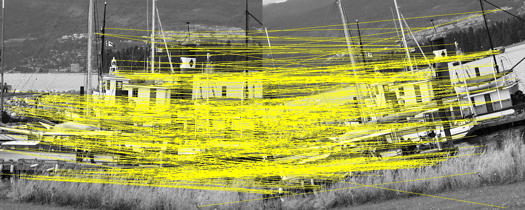
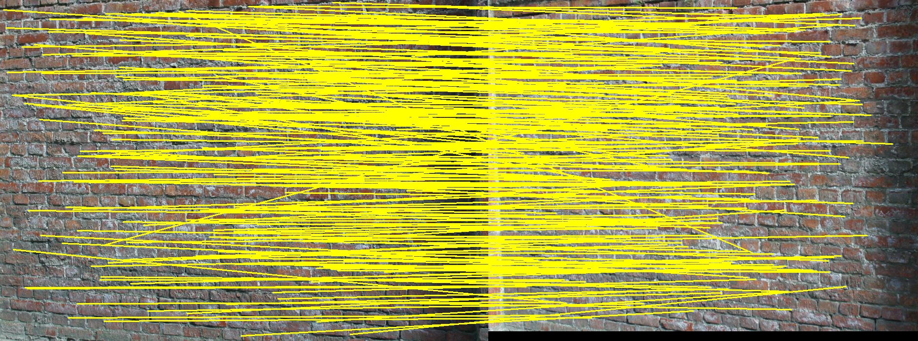
Since there are no exact corresponding relationships between all candidate nodes of two graphs normally, partial nodes are selected based on the criterion that if a candidate node has high similarity (inner product of feature vectors) with all candidate nodes from another graph, it is preferred to be chosen. Then all chosen nodes are connected, and the weights of edges are measured by the Euclidean distance between two corresponding nodes. The running time and matching error are calculated by the average results of five matching pairs (1 vs. 2, 2 vs. 3 …5 vs. 6) from the same picture set (Except set bike, we only record the results of 1 vs. 2, because other pairs in the set do not have enough nodes). The results are shown in Fig. 1 and Fig. 2. Visualization of the matching results are shown in Fig. 3.

Figure 1: Matching error

Figure 2: Matching time

(a) Boat

(b) Graf

(c) wall

Figure 3: Graphs from real images

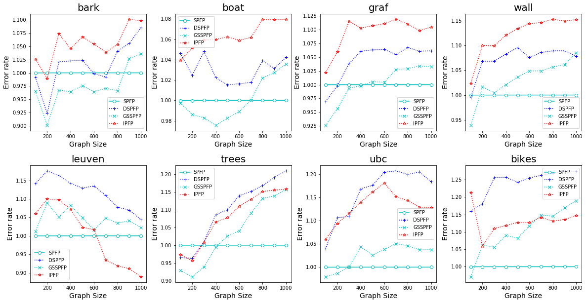
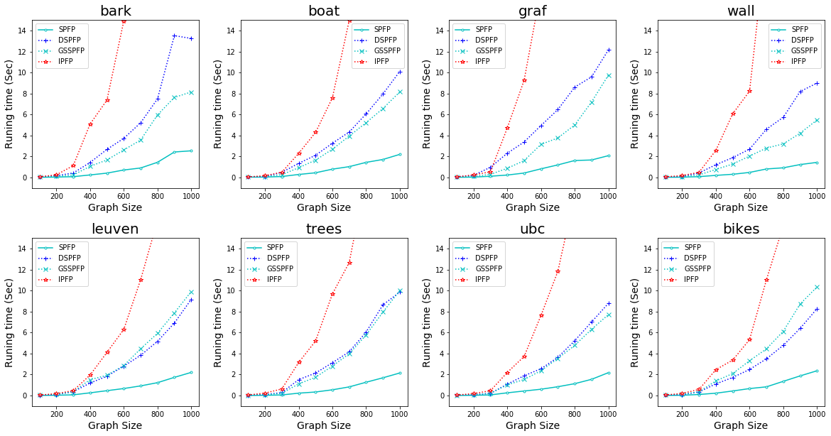
From Fig. 2, we can observe that SPFP is much faster than other graph matching algorithms. It takes about 2 seconds to match large graphs with size of 1000, while the other two algorithms need over 3 times more running time. Fig. 1 shows that SPFP achieves the lowest matching error in half of the experiments and also achieves a good performance in the other half of the experiments.

7.2.2 Image sequence

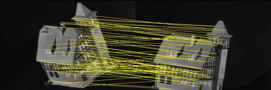
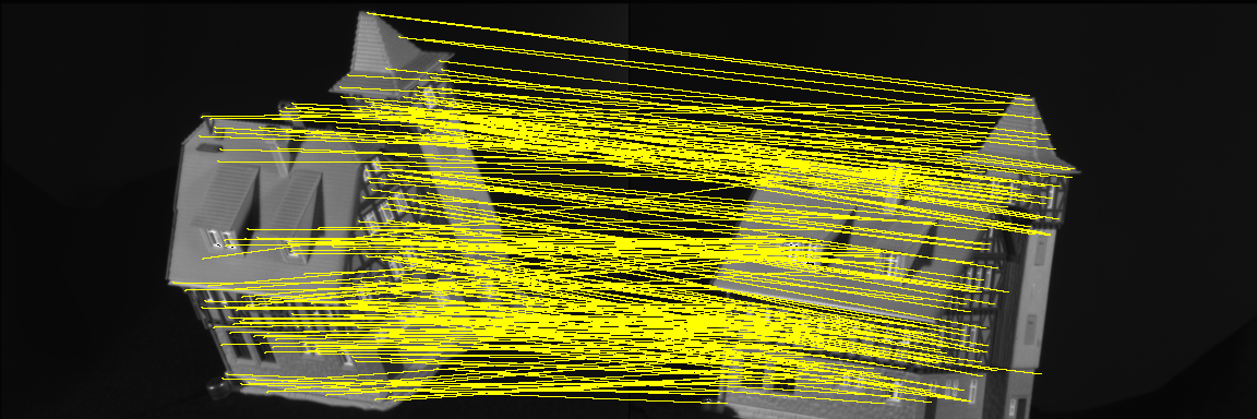
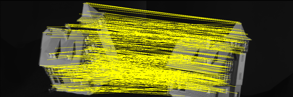
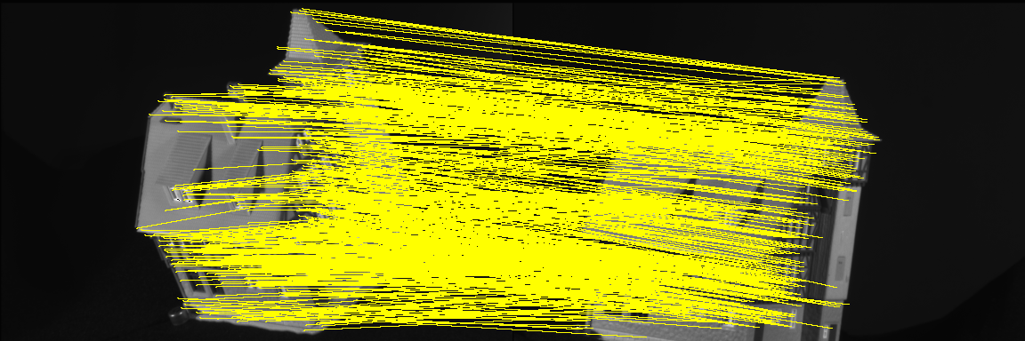
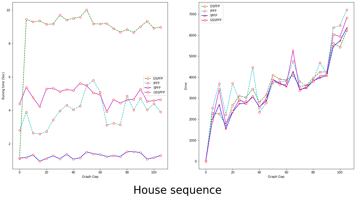
Weighted graphs are constructed from the CMU House sequence images in this set of experiments. The construction process is similar to the case of real image except that there are feature vectors and a selection step. All the key points (around 700) are extracted by the SIFT, and used as nodes of the graph. See Fig. 4 for visualization of the matching results. Matching pairs consist of the first image and subsequent images with 5 image sequence gaps (such as image 1 vs. image 2 and so on). The running time and matching error are recorded in Fig. 5 and Table 2. Again, the SPFP outperforms the others in term of speed and accuracy.

(a) 10% links

(b) 30% links

(c) 50% links

(d) 100% links

Figure 4: House matching results

Table 2: Graphs from house sequence

	DSPFP/SPFP			GSSPFP/SPFP			IPFP/SPFP
Running time	1.88			2.33			4.23
Matching error	1.02			1.03			1.11

Figure 5: House Matching

7.2.3 Randomly generated graphs

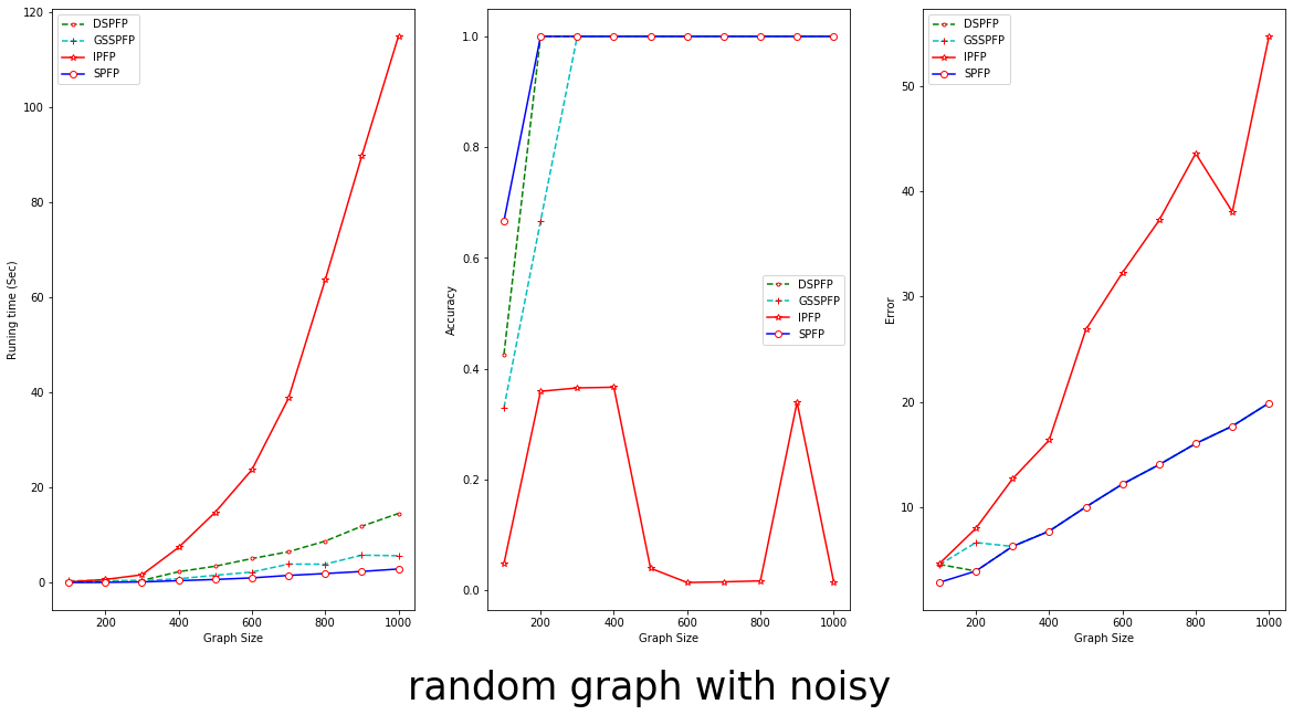
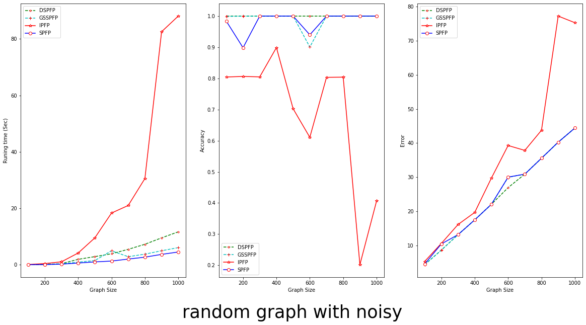
In this set of experiments, random weighted graphs are generated in the following way: $n$ pairs of numbers are randomly generated as the coordinates of nodes. The graphs with $10\%$ and $50\%$ connection rate are constructed. The weight of the edge represents the Euclidean distance between two corresponding nodes. Additionally, Two kinds of noise are added: $10\%$ nodes deletion and $n$ edges noise. The matching results are shown in Fig. Fig. 6 and 7. On this randomly generated example, the SPFP algorithm exhibits its robustness in terms of speed and accuracy again.

Figure 6: Connection rate = 0.1

Figure 7: Connection rate = 0.5

7.2.4 The effect of adaptive step size parameter

This example aims to examine the influence of using the adaptive step size parameter in the four algorithms. To construct sparse graphs, 500 nodes are generated from random coordinates and linked by the Delaunay triangulation method. Each set of experiments is repeated one hundred times to control the randomness. The matching results are shown in Fig. 8 and Table. 3.

Figure 8: APFP means adaptive projected fixed-point algorithms, and ASM represents adaptive spectra matching.

Table 3: Improvements from the adaptive step size

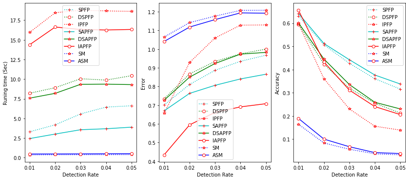
Algorithms	projection scheme	Time	Matching error	Accuracy
SPFP	softassign	35.0%	8.0%	3.5%
DSPFP	alternating projeciton	7.8%	1.2%	4.2%
IPFP	greedy projection	12.6%	36.7%	33.5%
SM	spectral projection	-29.8%	2.7%	17.2%

The figure and table show that the adaptive step size parameter strategy enhances the performance of projected fixed-point algorithms, except that ASM is slower than SM because of its different relaxation mentioned in Sec.3.1. Among algorithms with doubly stochastic constraints, the proposed SPFP/SAPFP shows a better performance consistently.

8 Conclusions

We propose an adaptive projected fixed-point method with dynamical softassign. Compared with other projected fixed-point methods, it achieves a high speed and keeps a comparable accuracy. The adaptive strategy of step size parameter significantly enhances the performance of graph matching algorithms based on the projected fixed-point method. The underlying mutual effects between graph size $n$ and inflation parameter $\beta$ are noticed in the tested examples, while theoretical analysis is still left unsolved. We find that there is a relation between the square root of graph size $\sqrt{n}$ and inflation parameter $\beta$ but lack theoretical proof. Therefore, rigorous mathematical analysis of the relationship is one of the future works.

References

- [1] D. Maio, D. Maltoni, A structural approach to fingerprint classification, in: Proceedings of 13th International Conference on Pattern Recognition, Vol. 3, IEEE, 1996, pp. 578–585.
- [2] L. Wiskott, J.-M. Fellous, N. Kruger, C. von der Malsburg, Face recognition by elastic bunch graph matching, Intelligent biometric techniques in fingerprint and face recognition 11 (5) (1999) 355–396.
- [3] C. Kotropoulos, A. Tefas, I. Pitas, Frontal face authentication using morphological elastic graph matching, IEEE Transactions on Image Processing 9 (4) (2000) 555–560.
- [4] Z. Lan, Y. Ma, L. Yu, L. Yuan, F. Ma, Aednet: Adaptive edge-deleting network for subgraph matching, Pattern Recognition (2022) 109033.
- [5] Z. Lan, B. Hong, Y. Ma, F. Ma, More interpretable graph similarity computation via maximum common subgraph inference, arXiv preprint arXiv:2208.04580 (2022).
- [6] D. Conte, P. Foggia, C. Sansone, M. Vento, Thirty years of graph matching in pattern recognition, International journal of pattern recognition and artificial intelligence 18 (03) (2004) 265–298.
- [7] J. Larrosa, G. Valiente, Constraint satisfaction algorithms for graph pattern matching, Mathematical structures in computer science 12 (4) (2002) 403–422.
- [8] L. P. Cordella, P. Foggia, C. Sansone, M. Vento, A (sub)graph isomorphism algorithm for matching large graphs, IEEE Trans Pattern Anal Mach Intell 26 (10) (2004) 1367–1372.
- [9] D. Conte, P. Foggia, C. Sansone, M. Vento, Thirty years of graph matching in pattern recognition, International journal of pattern recognition and artificial intelligence 18 (03) (2004) 265–298.
- [10] M. Cho, J. Lee, K. M. Lee, Reweighted random walks for graph matching, in: European Conference on Computer Vision, 2010.
- [11] S. Gold, A. Rangarajan, A graduated assignment algorithm for graph matching, IEEE Transactions on pattern analysis and machine intelligence 18 (4) (1996) 377–388.
- [12] M. Leordeanu, M. Hebert, R. Sukthankar, An integer projected fixed point method for graph matching and map inference, in: Advances in neural information processing systems, 2009, pp. 1114–1122.
- [13] Y. Lu, K. Huang, C.-L. Liu, A fast projected fixed-point algorithm for large graph matching, Pattern Recognition 60 (2016) 971–982.
- [14] S. Berretti, A. Del Bimbo, E. Vicario, A look-ahead strategy for graph matching in retrieval by spatial arrangement, in: 2000 IEEE International Conference on Multimedia and Expo. ICME2000. Proceedings. Latest Advances in the Fast Changing World of Multimedia (Cat. No. 00TH8532), Vol. 3, IEEE, 2000, pp. 1721–1724.
- [15] M. Leordeanu, M. Hebert, A spectral technique for correspondence problems using pairwise constraints, in: Tenth IEEE International Conference on Computer Vision (ICCV’05) Volume 1, Vol. 2, IEEE, 2005, pp. 1482–1489.
- [16] K.-C. Chang, S. Shao, D. Zhang, W. Zhang, Lovász extension and graph cut, Communications in Mathematical Sciences 19 (3) (2021) 761–786.
- [17] B. Shen, Q. Niu, S. Zhu, Fabricated pictures detection with graph matching, in: Proceedings of the 2020 2nd Asia Pacific Information Technology Conference, 2020, pp. 46–51.
- [18] E. L. Lawler, The quadratic assignment problem, Management science 9 (4) (1963) 586–599.
- [19] M. Zaslavskiy, F. Bach, J.-P. Vert, A path following algorithm for the graph matching problem, IEEE Transactions on Pattern Analysis and Machine Intelligence 31 (12) (2008) 2227–2242.
- [20] H. W. Kuhn, The hungarian method for the assignment problem, Naval research logistics quarterly 2 (1-2) (1955) 83–97.
- [21] A. Rangarajan, A. Yuille, E. Mjolsness, Convergence properties of the softassign quadratic assignment algorithm, Neural Computation 11 (6) (1999) 1455–1474.
- [22] R. Sinkhorn, P. Knopp, Concerning nonnegative matrices and doubly stochastic matrices, Pacific Journal of Mathematics 21 (2) (1967) 343–348.
- [23] Harville, A. David, Matrix algebra from a statistician’s perspective 10.1007/b98818 (2008).
- [24] S. Zhu, Numerical linear approximation involving radial basis functions, Ph.D. thesis, Oxford University, UK (2014).
- [25] I. J. Schoenberg, On certain metric spaces arising from euclidean spaces by a change of metric and their imbedding in hilbert space, Annals of mathematics (1937) 787–793.
- [26] S. Zhu, Compactly supported radial basis functions: how and why? (2012).