Symmetry restoration in the vicinity of neutron stars with a nonminimal coupling

Abstract

We propose a new model of scalarized neutron stars (NSs) realized by a self-interacting scalar field $\phi$ nonminimally coupled to the Ricci scalar $R$ of the form $F(\phi)R$. The scalar field has a self-interacting potential and sits at its vacuum expectation value $\phi_{v}$ far away from the source. Inside the NS, the dominance of a positive nonminimal coupling over a negative mass squared of the potential leads to a symmetry restoration with the central field value $\phi_{c}$ close to $0$. This allows the existence of scalarized NS solutions connecting $\phi_{v}$ with $\phi_{c}$ whose difference is significant, whereas the field is located in the vicinity of $\phi=\phi_{v}$ for weak gravitational stars. The Arnowitt-Deser-Misner mass and radius of NSs as well as the gravitational force around the NS surface can receive sizable corrections from the scalar hair, while satisfying local gravity constraints in the Solar system. Unlike the original scenario of spontaneous scalarization induced by a negative nonminimal coupling, the catastrophic instability of cosmological solutions can be avoided. We also study the cosmological dynamics from the inflationary epoch to today and show that the scalar field $\phi$ finally approaches the asymptotic value $\phi_{v}$ without spoiling a successful cosmological evolution. After $\phi$ starts to oscillate about the potential minimum, the same field can also be the source for cold dark matter.

I Introduction

Having the detection of gravitational waves from binary systems composed of black holes (BHs) and/or neutron stars (NSs) Abbott et al. (2016, 2017), we are now ready for testing physics on strong gravitational backgrounds in the strong field regime Berti et al. (2015, 2018); Barack et al. (2019). General Relativity (GR) is currently recognized as a fundamental theory describing the gravitational interaction, but it is not yet clear how much extent to GR is trustable in the vicinity of extreme compact objects. There are some alternative theories of gravity like scalar-tensor theories Horndeski (1974); Fujii and Maeda (2007); Deffayet et al. (2011); Kobayashi et al. (2011); Charmousis et al. (2012); Kase and Tsujikawa (2019); Kobayashi (2019) in which a new degree of freedom like a scalar field could modify the gravitational interaction through couplings to curvature invariants. Since the accuracy of GR has been well confirmed in the weak-field regimes, modified gravitational theories have to be constructed to be consistent with local gravity constraints in the Solar system De Felice and Tsujikawa (2010); Clifton et al. (2012); Joyce et al. (2015); Will (2014); Koyama (2016); Heisenberg (2019).

In the presence of a scalar field $\phi$ nonminimally coupled with the Ricci scalar $R$ of the form $F(\phi)R$, it is known that a phenomenon called spontaneous scalarization can occur for static and spherically symmetric NSs Damour and Esposito-Farese (1993), while recovering the GR behavior in the weak-field backgrounds. Spontaneous scalarization is an interesting phenomenon in that the large deviation from GR manifests itself on strong gravitational backgrounds Sotani and Kokkotas (2004); Sotani (2014); Minamitsuji and Silva (2016). In the presence of a scalar Gauss-Bonnet coupling, scalarization can occur for non-rotating and rotating BHs Doneva and Yazadjiev (2018a); Silva et al. (2018); Doneva and Yazadjiev (2018a); Antoniou et al. (2018, 2018, 2018); Minamitsuji and Ikeda (2019); Cunha et al. (2019); Dima et al. (2020); Herdeiro et al. (2021); Berti et al. (2021) as well as NSs Doneva and Yazadjiev (2018b). Spontaneous scalarization can take place with a scalar-gauge coupling $\alpha(\phi)F_{\mu\nu}F^{\mu\nu}/4$ for charged BHs Herdeiro et al. (2018); Fernandes et al. (2019) and charged stars Minamitsuji and Tsujikawa (2021). While the extension of spontaneous scalarization of NSs to the vector-field sector has been considered in the literature Annulli et al. (2019); Ramazanoğlu (2017, 2019); Kase et al. (2020a); Minamitsuji (2020), it has been argued that these models generically suffer from ghost or gradient instabilities Garcia-Saenz et al. (2021); Silva et al. (2022); Demirboğa et al. (2022).

In the original model of Damour and Esposito-Farese based on the nonminimal coupling $F(\phi)R$ Damour and Esposito-Farese (1993), the necessary conditions for the occurrence of NS scalarization are given by $F_{,\phi}(0)=0$ and $F_{,\phi\phi}(0)>0$, where $F_{,\phi}={\rm d}F/{\rm d}\phi$ and $F_{,\phi\phi}={\rm d}^{2}F/{\rm d}\phi^{2}$. In general, there is a nonvanishing scalar-field branch $\phi(r)\neq 0$ that depends on the radial distance $r$ besides a GR branch $\phi(r)=0$. The effective field mass squared around $\phi=0$ is given by $m_{\rm eff}^{2}(0)=-M_{\rm pl}^{2}F_{,\phi\phi}(0)R_{0}/2$, where $M_{\rm pl}$ is the reduced Planck mass and $R_{0}$ is the Ricci scalar at $\phi=0$. In the weak-field backgrounds, the field can stay in the GR branch due to the smallness of $R_{0}$. Inside extreme compact objects like NSs, the negative mass squared $m_{\rm eff}^{2}(0)<0$ induced by large values of $R_{0}$ can trigger a tachyonic instability toward the nontrivial branch $\phi(r)\neq 0$.

The typical choice of nonminimal couplings consistent with the first condition $F_{,\phi}(0)=0$ is $F(\phi)={\rm e}^{-\beta\phi^{2}/(2M_{\rm Pl}^{2})}$, where $\beta$ is a constant. To realize the second condition $F_{,\phi\phi}(0)>0$, i.e., $m_{\rm eff}^{2}(0)<0$, we require that $\beta<0$. The studies in Refs. Harada (1998); Novak (1998); Silva et al. (2015) have shown that spontaneous scalarization can occur for the nonminimal coupling in the range $\beta\leq-4.35$, irrespective of the NS equation of state (EOS). On the other hand, the binary pulsar measurements of an energy loss through the dipolar radiation have put the bound $\beta\geq-4.5$ Freire et al. (2012); Shao et al. (2017). Then, the coupling constant $\beta$ is constrained to be in a limited range.

If we apply the above nonminimally coupled theory to cosmology, it is known that the scalar field is subject to a tachyonic instability for negative values of $\beta$ required for the occurrence of spontaneous scalarization Damour and Nordtvedt (1993a, b). Around $\phi=0$, the effective field mass squared is estimated as $m_{\rm eff}^{2}(0)\simeq\beta R_{0}/2$, so that $m_{\rm eff}^{2}(0)<0$ for $\beta<0$ expect the radiation-dominated era (where $R_{0}=0$). During inflation in which the Hubble expansion rate $H$ is nearly constant, we have $m_{\rm eff}^{2}(0)\simeq 6\beta H^{2}$ and hence the negative coupling of order $\beta\simeq-5$ leads to the exponential growth of $\phi$. This spoils the success of the standard inflationary paradigm. We note that the initial field value at the onset of inflation cannot be tuned to 0 due to the presence of scalar-field perturbations $\delta\phi$. Indeed, the perturbations $\delta\phi$ relevant to the scales of observed CMB temperature anisotropies are exponentially amplified after the Hubble radius crossing during inflation. The scalar field also increases during matter and dark energy dominated epochs. Hence the GR solution $\phi=0$ is not a cosmological attractor and the Solar-system constraints would be easily violated. The similar instability of cosmological solutions is present for spontaneously scalarized BHs realized by a scalar Gauss-Bonnet coupling Anson et al. (2019a); Franchini and Sotiriou (2020); Antoniou et al. (2021).

There have been several attempts to reconcile NS spontaneous scalarizations with cosmology. One scenario is to take into account higher-order polynomial corrections (like ${\cal O}(\phi^{4})$) to the nonminimal coupling function $F(\phi)$ Anderson et al. (2016). There is also a scalarization scenario based on a disformal coupling between the scalar field $\phi$ and matter Silva and Minamitsuji (2019). In this case, however, it was shown that the large disformal coupling required for the cosmological evolution toward $\phi=0$ works to suppress the occurrence of spontaneous scalarization.

The other scalarization scenario, which is called an “asymmetron” model Chen et al. (2015), is to introduce a mass term of the scalar field in the original model of Damour and Esposito-Farese, where the effective potential of the scalar field $\phi$ could have a global minimum. In this scenario, there is a nonvanishing global minimum and the scalar field moves toward this point due to tachyonic instability during inflation. After the Universe enters the radiation-dominated epoch, the scalar field decouples from matter and the global minimum shifts back to the origin of the effective potential. As the Universe expands further during the matter era, the Hubble parameter drops below the mass of $\phi$. Then the scalar field undergoes a damped oscillation, after which the cosmological evolution approaches that of GR. Hence GR is a cosmological attractor in the present Universe, while in local high-density regions spontaneous scalarization can occur as in the original Damour-Esposito-Farese model. Moreover, the oscillating scalar field can be a candidate for cold dark matter (CDM).

There is also another possibility for introducing a coupling between $\phi$ and the inflaton $\chi$ of the form $g^{2}\phi^{2}\chi^{2}/2$, where $g$ is a coupling constant Anson et al. (2019b). Then the effective field mass squared $m_{\rm eff}^{2}(\phi)$ can be largely positive during inflation, in which case $\phi$ decreases exponentially toward 0. After the end of the radiation-dominated era, the field $\phi$ starts to increase by the tachyonic mass. Provided that the suppression of $\phi$ during inflation occurs sufficiently, however, it is possible that today’s value of $\phi$ is below the limit constrained by Solar-system experiments. Although the four-point coupling $g$ larger than the order $10^{-5}$ can lead to viable cosmological dynamics including the reheating epoch after inflation Nakarachinda et al. (2023), the nonminimal coupling constant $\beta$ still needs to be in a limited negative range.

In this paper, we propose a new mechanism for NS scalarizations realized by the presence of a self-interacting potential of the form $V(\phi)=m^{2}f_{B}^{2}[1+\cos(\phi/f_{B})]$ besides the nonminimal coupling ${\rm e}^{-\beta\phi^{2}/(2M_{\rm Pl}^{2})}R$, where $m$ and $f_{B}$ are constants with mass dimension. In this setup, the field $\phi$ is in a ground state at the vacuum expectation value (VEV) $\phi_{v}=\pi f_{B}$ in the asymptotic region far away from a NS. At $\phi=0$ the bare potential $V(\phi)$ has a negative mass squared $-m^{2}$, but the positive nonminimal coupling constant ($\beta>0$) gives rise to a positive contribution $\beta R_{0}/2$ to the effective mass squared as $m_{\rm eff}^{2}(0)=-m^{2}+\beta R_{0}/2$. In the high-curvature region with $m_{\rm eff}^{2}(0)>0$, the field $\phi$ can stay in the vicinity of $\phi=0$. The transition to the region close to $\phi=0$ should occur inside the NS for the coupling $\beta>{\cal O}(0.1)$ with $m={\cal O}(10^{-11}\,{\rm eV})$, where the Compton radius $m^{-1}={\cal O}(10\,{\rm km})$ corresponds to the typical size of NSs. We will show the existence of field profiles connecting the internal solution ($\phi\simeq 0$) to the external solution far outside the star ($\phi\simeq\phi_{v}$). A conceptually similar model was proposed in Ref. Babichev et al. (2022), where scalarized BHs were induced by the scalar Gauss-Bonnet coupling with a symmetry-breaking potential.

We note that the structure of our model is similar to the symmetron scenario Hinterbichler and Khoury (2010), which was proposed as one of the screening mechanisms of fifth forces in local regions of the Universe. The similarity is that positive nonminimal couplings are used to restore the symmetry at $\phi=0$ at high density and that the tachyonic mass of the potential breaks the symmetry to reach the state at $\phi=\phi_{v}$ at low density. In the symmetron model the scalar field is relevant to the late-time cosmic acceleration (i.e., dark energy), so that the scalar field mass is as small as $m={\cal O}(10^{-30}~{}{\rm eV})$. The fifth force can be suppressed for $\phi$ close to 0, but it propagates once $\phi$ reaches the region close to $\phi_{v}$ (see Refs. Burrage and Sakstein (2018); Brax et al. (2021) for laboratory tests of the symmetron). In our model the typical mass scale is as large as $m={\cal O}(10^{-11}~{}{\rm eV})$, in which case it is possible to satisfy local gravity constraints even for $\phi$ close to $\phi_{v}$. In the vicinity of NSs, the scalar field can reach the region close to $\phi=0$ and hence the spherically symmetric solutions in strong gravity regimes exhibit differences from those in weak gravity regimes. Cosmologically, the scalar field can also behave as CDM after the symmetry breaking. These properties are different from those in the symmetron model. Our model is also different from the asymmetron model mentioned above in that the Universe approaches the GR vacuum at $\phi=0$ but not the one at $\phi=\phi_{v}$ in late-time/low density regimes.

In our model, the nonminimal coupling constant $\beta$ is positive and the effective mass squared $m_{\rm eff}^{2}(0)=-m^{2}+\beta R_{0}/2$ at $\phi=0$ is positive in the early cosmological epoch satisfying $\beta R_{0}/2>m^{2}$. Then, during inflation, the scalar field $\phi$ can decrease exponentially toward 0. After $\beta R_{0}/2$ drops below $m^{2}$ in the radiation-dominated era, the field $\phi$ should exhibit tachyonic growth toward the ground state at $\phi=\phi_{v}$. Indeed, we will show that the field settles down the potential minimum by today without violating a successful cosmic expansion history. After $\phi$ starts to oscillate around $\phi_{v}$, the same field can also work as the source for (a portion of) CDM.

In weak gravitational objects like the Sun, the Ricci scalar $R$ inside the star is small in comparison to that in NSs and hence $m_{\rm eff}^{2}$ is negative in the vicinity of $\phi=0$. In such cases, the scalar field is in the region close to $\phi=\phi_{v}$ both inside and outside the star. We will obtain the field profile and post-Newtonian parameter and put bounds on the scale $f_{B}$ from Solar-system tests on local gravity. Using these constrained values of $f_{B}$, we numerically construct scalarized NS solutions with nontrivial profiles of the scalar field and compute the effect on the Arnowitt-Deser-Misner (ADM) mass and radius of NSs as well as modifications of gravity around the surface of star. We will show that the difference of the ADM mass of scalarized NSs from that in GR can exceed more than 10 %. The modified gravitational interaction induced in our scenario may be detectable in future observations of gravitational waves and other measurements on the strong field regimes.

This paper is organized as follows. In Sec. II, we present our new model of NS scalarizations and discuss its basic structure. In Sec. III, we study the cosmological dynamics of the nonminimally coupled scalar field from an inflationary epoch to today and show that the field is eventually stabilized at $\phi=\phi_{v}$ without preventing the cosmic expansion history. In Sec. IV, we derive the field profile for a constant density star on weak gravitational backgrounds and place bounds on model parameters from Solar-system constraints. In Sec. V, we obtain the scalar-field solution for NSs and study its effect on the modification of gravitational interactions. Sec. VI is devoted to conclusions.

II Models with NS scalarizations

We consider theories given by the action

$${\cal S}=\int{\rm d}^{4}x\sqrt{-g_{J}}\left[\frac{M_{\rm Pl}^{2}}{2}F(\phi)R+\omega(\phi)X-V(\phi)\right]+{\cal S}_{m}(g_{\mu\nu},\Psi_{m})\,,$$ (1)

where $g_{J}$ is a determinant of the metric tensor $g_{\mu\nu}$, $M_{\rm pl}$ is a constant having the dimension of mass, $F$ is a function of $\phi$, $R$ is the Ricci scalar, $X=-(1/2)g^{\mu\nu}\nabla_{\mu}\phi\nabla_{\nu}\phi$ is a scalar kinetic term with the covariant derivative operator $\nabla_{\mu}$, $V(\phi)$ is a scalar potential, and

$$\omega(\phi)=\left(1-\frac{3M_{\rm Pl}^{2}F_{,\phi}^{2}}{2F^{2}}\right)F\,,$$ (2)

with $F_{,\phi}\equiv{\rm d}F/{\rm d}\phi$ and so on. The action ${\cal S}_{m}$ incorporates the contributions of matter fields $\Psi_{m}$ inside the NS. Note that in the case $F(\phi)=1$ the constant $M_{\rm Pl}$ represents the reduced Planck mass ($M_{\rm Pl}=2.435\times 10^{18}$ GeV).

The equations of motion for the metric and scalar field are given, respectively, by

$$M_{\rm Pl}^{2}\left[F(\phi)G_{\mu\nu}+\Box F(\phi)g_{\mu\nu}-\nabla_{\mu}\nabla_{\nu}F(\phi)\right]-\omega(\phi)\left(\nabla_{\mu}\phi\nabla_{\nu}\phi+Xg_{\mu\nu}\right)+g_{\mu\nu}V(\phi)=T_{\mu\nu},$$ (3)

$$\omega(\phi)\Box\phi-\omega_{,\phi}(\phi)X+\frac{M_{\rm Pl}^{2}}{2}F_{,\phi}(\phi)R-V_{,\phi}(\phi)=0,$$ (4)

where $T_{\mu\nu}$ represents the energy-momentum tensor of matter in the Jordan frame defined by

$$T_{\mu\nu}\equiv-\frac{2}{\sqrt{-g_{J}}}\frac{\delta{\cal S}_{m}}{\delta g^{\mu\nu}}.$$ (5)

Acting the operator $\nabla^{\mu}$ on Eq. (3) and using Eq. (4), we obtain the conservation law of matter as

$$\nabla^{\mu}T_{\mu\nu}=0.$$ (6)

We consider the nonminimal coupling chosen by Damour and Esposito-Farese Damour and Esposito-Farese (1993)

$$F(\phi)={\rm e}^{-\beta\phi^{2}/(2M_{\rm pl}^{2})}\,,$$ (7)

where $\beta$ is a dimensionless constant. From Eq. (2), we have

$$\omega(\phi)=\left(1-\frac{3\beta^{2}\phi^{2}}{2M_{\rm Pl}^{2}}\right)F\,.$$ (8)

Under a conformal transformation of the action (1) to the Einstein frame, the theory with $V(\phi)=0$ recasts the one originally advocated in Ref. Damour and Esposito-Farese (1993) (see the Appendix of Ref. Kase et al. (2020a)). In the following, we will perform all the analysis in the Jordan frame action (1).

Let us first revisit the case of standard NS spontaneous scalarization in the absence of the scalar potential, i.e.,

$$V(\phi)=0\,.$$ (9)

Then, there is the branch $\phi=0$ as one of the solutions to Eq. (4). For this solution, Eq. (3) reduces to the Einstein equation $M_{\rm Pl}^{2}G_{\mu\nu({\rm GR})}=T_{\mu\nu({\rm GR})}$ in GR. In regions of the large curvature $R$, it is possible to have a nontrivial branch with $\phi\neq 0$ besides the GR branch $\phi=0$. If we consider a small perturbation $\delta\phi$ about the GR solution, the perturbation obeys $\square\delta\phi-m_{\rm eff}^{2}(0)\delta\phi=0$, where $m_{\rm eff}^{2}(0)=-M_{\rm pl}^{2}F_{,\phi\phi}(0)R_{0}/2$ and $R_{0}$ is the Ricci scalar in the GR background at $\phi=0$. Provided that $F_{,\phi\phi}(0)>0$ with $R_{0}>0$, the GR branch is subject to tachyonic instability due to the negative mass squared $m_{\rm eff}^{2}(0)$. For $\beta<0$, there is a possibility for NSs to acquire a scalar hair after the spontaneous growth of $\phi$ toward the other nontrivial branch, whose phenomenon is dubbed spontaneous scalarization.

As mentioned in Sec. I, the nonminimal coupling constant $\beta$ needs to be in the limited range $-4.5\leq\beta\leq-4.35$ in the original model of Ref. Damour and Esposito-Farese (1993). Here, the upper limit of $\beta$ arises for the occurrence of spontaneous scalarization Harada (1998); Novak (1998), whereas the lower bound comes from binary pulsar measurements Freire et al. (2012); Shao et al. (2017). For such negative values of $\beta$, there is a tachyonic instability of the field $\phi$ on the cosmological background and hence GR solution $\phi=0$ is not an attractor. This instability is particularly prominent during the inflationary epoch to destroy the background evolution. Then, the successful cosmic expansion history is spoiled by the negative nonminimal coupling with $V(\phi)=0$.

The story is different for the positive nonminimal coupling with a self-interacting scalar potential $V(\phi)$. For concreteness, we consider a potential of the pseudo Nambu-Goldstone boson (pNGB), which is given by

$$V(\phi)=m^{2}f_{B}^{2}\left[1+\cos\left(\frac{\phi}{f_{B}}\right)\right]\,,$$ (10)

where $m$ and $f_{B}$ are constants having the dimension of mass. This potential has a reflection symmetry with respect to $\phi=0$. To choose either the ground state at $\phi=\pi f_{B}$ or $\phi=-\pi f_{B}$ means the breaking of the reflection symmetry. We will choose the positive VEV $\phi_{v}=\pi f_{B}$ as a symmetry-breaking ground state. Note that in order to test our idea, the form of the scalar field potential may not be restricted to a particular from as Eq. (10). We can consider other symmetry-breaking potentials like $V(\phi)=h^{2}(\phi^{2}-\phi_{v}^{2})^{2}$, where $h$ and $\phi_{v}$ are constants. Indeed, so long as the potential has a local maximum at $\phi=0$ and a global minimum at $\phi\neq 0$, it is sufficient for our purpose of the construction of a viable model. We choose the particular pNGB potential (10) for an illustration.

Around $\phi=0$, the potential (10) has a negative mass squared $-m^{2}$. Since the nonmininal coupling $M_{\rm Pl}^{2}F(\phi)R/2$ is present, the squared effective mass of the field at $\phi=0$ yields

$$m_{\rm eff}^{2}(0)=-m^{2}+\frac{\beta}{2}R_{0}\,.$$ (11)

Due to the largeness of $R_{0}$ in regions of the high density, the positive nonminimal coupling constant $\beta$ can lead to the symmetry restoration at $\phi=0$. This occurs if $\beta R_{0}/2$ exceeds the negative mass squared $-m^{2}$. In regions of the low density, the effect of $\beta R_{0}/2$ on $m_{\rm eff}^{2}(0)$ should be unimportant relative to the contribution $-m^{2}$. Hence the scalar field would acquire the VEV $\phi_{v}=\pi f_{B}$ on weak gravitational backgrounds. This scalar-field configuration is different from that arising from standard NS spontaneous scalarization with $V(\phi)=0$, in that the scalar field is in the symmetry-restored state $\phi=0$ around the center of star while $\phi$ approaches the asymptotic value $\phi_{v}=\pi f_{B}$ far away from the star.

For a star with the mean density $\rho$ and pressure $P$, the Ricci scalar $R$ at $\phi=0$ is of order $R\simeq(\rho-3P)/M_{\rm Pl}^{2}$. Then, the critical value of $\beta$ corresponding to $m_{\rm eff}^{2}(0)=0$ can be estimated as

$$\beta_{c}=\frac{2m^{2}M_{\rm Pl}^{2}}{\rho-3P}=0.28\left(\frac{10^{15}~{}{\rm g/cm}^{3}}{\rho-3P}\right)\left(\frac{m}{10^{-11}~{}{\rm eV}}\right)^{2}\,.$$ (12)

Note that, for $m={\cal O}(10^{-11}~{}{\rm eV})$, the Compton radius of $\phi$ is of ${\cal O}(10\,{\rm km})$, i.e., the typical the size of NSs. For $\beta>\beta_{c}$ we have $m_{\rm eff}^{2}(0)>0$, and the scalar field can be in the symmetry-restored state at $\phi=0$. For $\beta<\beta_{c}$, the state at $\phi=0$ becomes unstable and hence the solution should approach the ground state at $\phi=\phi_{v}$. The typical central density of NSs is around $\rho=10^{15}~{}{\rm g/cm}^{3}$, so the mass of order $m=10^{-11}~{}{\rm eV}$ gives rise to the critical coupling $\beta_{c}$ around $\beta_{c}=0.1\sim 1$.

On the Friedmann-Lemaître-Robertson-Walker (FLRW) cosmological background, the scalar field can be in the state $\phi=0$ in the early Universe satisfying the condition $\beta R_{0}/2>m^{2}$. After the term $\beta R_{0}/2$ drops below $m^{2}$ along the cosmic expansion, however, the field should evolve to the ground state at $\phi=\phi_{v}$ since $m_{\rm eff}^{2}(0)$ becomes negative. In Sec. III, we study cosmology in the above model in details and show that $\phi$ sufficiently approaches the potential minimum by today.

III Cosmology with positive nonminimal coupling

We study the cosmological dynamics of the scalar field $\phi$ from the inflationary epoch to today for the theory given by the action (1). A spatially-flat FLRW background is given by the line element

$${\rm d}s^{2}=g_{\mu\nu}{\rm d}x^{\mu}{\rm d}x^{\nu}=-{\rm d}t^{2}+a^{2}(t)\delta_{ij}{\rm d}x^{i}{\rm d}x^{j}\,,$$ (13)

where the scale factor $a(t)$ depends on the cosmic time $t$. Then, the gravitational and scalar-field equations of motion are

$$3FH^{2}M_{\rm Pl}^{2}=-3M_{\rm Pl}^{2}HF_{,\phi}\dot{\phi}+\frac{1}{2}\omega\dot{\phi}^{2}+V+\rho\,,$$ (14)

$$F\left(2\dot{H}+3H^{2}\right)M_{\rm Pl}^{2}=-M_{\rm Pl}^{2}\left[F_{,\phi}(\ddot{\phi}+2H\dot{\phi})+F_{,\phi\phi}\dot{\phi}^{2}\right]-\frac{1}{2}\omega\dot{\phi}^{2}+V-P\,,$$ (15)

$$\ddot{\phi}+3H\dot{\phi}-\frac{3M_{\rm Pl}^{2}F_{,\phi}}{\omega}\left(\dot{H}+2H^{2}\right)+\frac{\omega_{,\phi}\dot{\phi}^{2}}{2\omega}+\frac{V_{,\phi}}{\omega}=0\,,$$ (16)

where $\rho$ and $P$ are the density and pressure of the inflaton field and/or perfect fluids, $H=\dot{a}/a$ is the Hubble parameter, and a ‘dot’ represents the derivative with respect to $t$, and $\omega_{,\phi}\equiv{\rm d}\omega/{\rm d}\phi$, $V_{,\phi}\equiv{\rm d}V/{\rm d}\phi$, and so on. Note that $F_{,\phi}=-\beta\phi F/M_{\rm Pl}^{2}$ and $F_{,\phi\phi}=\beta(\beta\phi^{2}-M_{\rm Pl}^{2})F/M_{\rm Pl}^{4}$, and in the regime $|\phi|\ll M_{\rm Pl}$, $\omega_{,\phi}/\omega\simeq-\beta(1+3\beta)\phi/M_{\rm Pl}^{2}$.

III.1 Evolution during inflation and reheating

To study the cosmological dynamics during inflation, we incorporate a canonical inflaton field $\chi$ with the potential $U(\chi)$. Then, we have $\rho=\dot{\chi}^{2}/2+U(\chi)$ and $P=\dot{\chi}^{2}/2-U(\chi)$ in Eqs. (14) and (15). The inflaton field obeys the continuity equation $\dot{\rho}+3H(\rho+P)=0$, i.e.,

$$\ddot{\chi}+3H\dot{\chi}+U_{,\chi}=0\,,$$ (17)

where $U_{,\chi}\equiv{\rm d}U/{\rm d}\chi$. The kinetic and potential energy of the field $\phi$ should be suppressed relative to $U(\chi)$ during inflation. Let us consider the typical Hubble scale of inflation of order $H\sim 10^{14}$ GeV. Since $V(\phi)$ is at most of order $m^{2}f_{B}^{2}$, we have $V(\phi)\lesssim m^{2}f_{B}^{2}\ll H^{2}M_{\rm Pl}^{2}\sim U(\chi)$ for the mass scale $m\sim 10^{-11}$ eV with $f_{B}\lesssim M_{\rm Pl}$. Provided that the condition $|\omega_{,\phi}|\dot{\phi}^{2}\ll H^{2}M_{\rm Pl}^{2}|F_{,\phi}|$ holds together with the slow-roll condition $|\dot{H}|\ll H^{2}$, Eq. (16) is approximately given by

$$\ddot{\phi}+3H\dot{\phi}+\frac{1}{\omega}\left[6\beta FH^{2}\phi-m^{2}f_{B}\sin\left(\frac{\phi}{f_{B}}\right)\right]\simeq 0\,.$$ (18)

We are interested in the coupling range $\beta\gtrsim 0.1$ with $m$ of order $10^{-11}$ eV. For $\phi\gtrsim f_{B}$, since $H\gg m$, the term $6\beta FH^{2}\phi$ dominates over $m^{2}f_{B}\sin(\phi/f_{B})$ during inflation. This is also the case for $0<\phi\ll f_{B}$ as $m^{2}f_{B}\sin(\phi/f_{B})\simeq m^{2}\phi$ in this regime. Then, during inflation, Eq. (18) approximately reduces to

$$\ddot{\phi}+3H\dot{\phi}+\frac{6\beta FH^{2}}{\omega}\phi\simeq 0\,,$$ (19)

and the contribution of the pNGB scalar potential to the background Eqs. (14)-(15) can be completely neglected. Provided that the scalar field is in the range $\beta\phi^{2}/M_{\rm Pl}^{2}\ll 1$, we have $F\simeq 1$ and $\omega\simeq 1$. On using the approximation that $H$ is constant during inflation, the dominant solution to Eq. (19) is given by

$$\phi\propto \exp\left(-\frac{3}{2}Ht\right)\cos(\Omega_{0}t+\theta_{0}) \beta>3/8)$$ (if  , (20)

$$\phi\propto \exp\left[-\frac{3}{2}\left(1-\sqrt{1-\frac{8}{3}\beta}\right)Ht\right] \beta<3/8)$$ (if  , (21)

where $\Omega_{0}=\sqrt{6\beta-9/4}\,H$ and $\theta_{0}$ is an arbitrary constant. For $\beta>3/8$, the field $\phi$ exhibits a damped oscillation with the amplitude rapidly decreasing as $|\phi|\propto\exp(-3Ht/2)$. If the total number of e-foldings during inflation is $N=\int_{0}^{t}H{\rm d}t\simeq Ht=60$, the amplitude of $\phi$ at the end of inflation is $8\times 10^{-40}$ times as small as that at the onset of inflation. For $0<\beta<3/8$, $\phi$ decreases without oscillations according to Eq. (21). If $\beta<0$, the scalar field increases as $\phi\propto\exp[(3/2)(\sqrt{1-8\beta/3}-1)Ht]$.

As the inflaton potential, we consider the $\alpha$-attractor type given by

$$U(\chi)=\frac{3}{4}\alpha M^{2}M_{\rm Pl}^{2}\left[1-\exp\left(-\sqrt{\frac{2}{3\alpha}}\frac{\chi}{M_{\rm Pl}}\right)\right]^{2}\,,$$ (22)

where $\alpha$ is a positive constant Kallosh et al. (2013). For $\alpha=1$, the potential (22) is equivalent to that of Starobinky inflation Starobinsky (1980) in the Einstein frame De Felice and Tsujikawa (2010). The field $\chi$ at the end of inflation can be determined by the condition $\epsilon_{V}=(M_{\rm Pl}^{2}/2)(V_{,\chi}/V)^{2}=1$, i.e., $\chi_{f}=0.940M_{\rm Pl}$. Cosmic acceleration occurs in the region where $\chi\gtrsim M_{\rm Pl}$, which is followed by the reheating stage driven by the oscillation of $\chi$ around $\chi=0$. From the Planck normalization of curvature perturbations generated during inflation, the mass $M$ is constrained to be around $M\simeq 10^{-5}M_{\rm Pl}$. In our numerical simulations we will choose the potential (22) with $\alpha=1$, but the evolution of $\phi$ during inflation and reheating is similar for any other slow-roll inflaton potentials which can be approximated by $U(\chi)\simeq M^{2}\chi^{2}/2$ in the vicinity of $\chi=0$. Indeed, the analytic solutions to $\phi$ given by Eqs. (20) and (21) during inflation as well as those during reheating derived later in Eqs. (26) and (27) are insensitive to the change of inflaton potentials.

In Fig. 1, we plot the evolution of $|\phi|/M_{\rm Pl}$ during inflation and reheating for $\beta=1,0.1,-1$ with $m=10^{-11}$ eV and $M=10^{-5}M_{\rm Pl}$. The initial conditions are chosen to be $\chi_{i}=5.365M_{\rm Pl}$, $\dot{\chi}_{i}=0$, $\phi_{i}=0.5M_{\rm Pl}$, and $\dot{\phi}_{i}=0$. For $\beta=1$, we can confirm that the amplitude of $\phi$ during inflation decreases as $|\phi|\propto\exp(-3Ht/2)$ with oscillations. In this simulation the number of e-foldings acquired during inflation is $N\simeq 60$, so the amplitude of $\phi$ at the end of inflation is of order $|\phi_{f}|\simeq|\phi_{i}|\exp(-90)\simeq 10^{-40}M_{\rm Pl}$. This rapid decrease of $\phi$ toward 0 is the outcome of a positive mass squared larger than $H^{2}$ induced by the nonminimal coupling with $\beta>3/8$. Due to the strong suppression of $\phi$, the dynamics of inflation driven by the $\chi$-field potential energy $U(\chi)$ is not affected by the presence of $\phi$. For $\beta=0.1$, the analytic estimation (21) shows that the field $\phi$ decreases as $|\phi|\propto\exp(-0.215Ht)$, so that $|\phi_{f}|\simeq 10^{-6}M_{\rm Pl}$ at the end of inflation. Even in this case, the dynamics of inflation is hardly modified by the field $\phi$.

When $\beta=-1$, the field $\phi$ grows as $\phi\propto\exp(1.372Ht)$ from the onset of inflation, the slow-roll inflation is prevented by the rapid increase of $\dot{\phi}^{2}$ (see Fig. 1). In particular, the epoch of cosmic acceleration soon comes to end by the negative coupling $\beta\simeq-5$ used for the occurrence of spontaneous scalarization with $V(\phi)=0$. In our setup, the presence of the self-interacting potential $V(\phi)$ with a positive nonminimal coupling $\beta$ allows a possibility for realizing a positive effective field mass squared around $\phi=0$. As discussed above, for $\beta>{\cal O}(0.1)$, the field $\phi$ decreases toward the local minimum of its effective potential ($\phi=0$) during inflation.

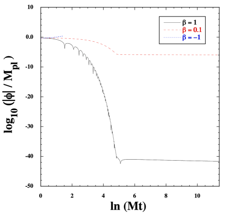
Figure 1: Evolution of $|\phi|/M_{\rm Pl}$ versus $\ln(Mt)$ during inflation and reheating for $\beta=1,0.1,-1$ with $m=1.0\times 10^{-11}$ eV and $M=1.1\times 10^{-5}M_{\rm Pl}$. We choose the $\alpha$-attractor potential (22) with $\alpha=1$ and the decay constant $\Gamma=10^{8}$ GeV. The initial conditions of scalar fields are $\chi_{i}=5.365M_{\rm Pl}$, $\dot{\chi}_{i}=0$, $\phi_{i}=0.5M_{\rm Pl}$, and $\dot{\phi}_{i}=0$. The integration is performed by the time at which the energy density of inflaton drops below that of radiation.

After inflation, the inflaton field $\phi$ should decay to radiation. To study the dynamics of $\phi$ during reheating, we incorporate the Born decay term $\Gamma\dot{\chi}$ in Eq. (17) as

$$\ddot{\chi}+\left(3H+\Gamma\right)\dot{\chi}+U_{,\chi}=0\,,$$ (23)

where $\Gamma$ is a constant. The radiation density $\rho_{r}$ obeys the differential equation

$$\dot{\rho}_{r}+4H\rho_{r}=\Gamma\dot{\chi}^{2}\,.$$ (24)

The energy density $\rho$ and pressure $P$ in Eqs. (14) and (15) should be also modified to $\rho=\dot{\chi}^{2}/2+U(\chi)+\rho_{r}$ and $P=\dot{\chi}^{2}/2-U(\chi)+\rho_{r}/3$, respectively. We numerically solve Eqs. (14)-(15) and (23)-(24) by using the field values $\chi_{f}$, $\phi_{f}$, and their time derivatives at the end of inflation as the initial conditions of the reheating period. We take the radiation into account from the end of inflation and integrate the background equations of motion by the time at which the inflaton energy density drops below $\rho_{r}$. For the mass $m$ of order $10^{-11}$ eV the condition $m^{2}f_{B}^{2}\ll H^{2}M_{\rm Pl}^{2}$ is satisfied in the standard reheating scenario, and it is a good approximation to neglect the contributions of the potential energy $V(\phi)$ to the background equations of motion.

The inflaton potential is approximated as $U(\chi)\simeq M^{2}\chi^{2}/2$ around $\chi=0$. The reheating stage driven by the oscillating $\chi$ field corresponds to a temporal matter era with $a\propto t^{2/3}$ and $H=2/(3t)$. As long as the field $\phi$ sufficiently approaches $0$ during inflation, Eq. (16) approximately reduces to

$$\ddot{\phi}+\frac{2}{t}\dot{\phi}+\frac{2\beta}{3t^{2}}\phi\simeq 0\,.$$ (25)

The dominant solution to this equation is given by

$$\phi\propto t^{-1/2}\cos\left(\sqrt{\frac{8\beta-3}{12}}\ln(Mt)+\theta_{0}\right) \beta>3/8)$$ (if  , (26)

$$\phi\propto t^{-(1-\sqrt{1-8\beta/3})/2} \beta<3/8)$$ (if  . (27)

The time $t_{f}$ at the beginning of reheating is related to the Hubble parameter at the end of inflation $H_{f}$, as $t_{f}\simeq 1/H_{f}$. The reheating period ends around the time $t_{R}\simeq 1/\Gamma$, after which the energy density of radiation dominates over that of the inflaton field $\chi$. Since the evolution of $\phi$ during inflation is given by Eqs. (20)-(21), the amplitude of $\phi$ at which the radiation-dominated epoch commences can be estimated as

$$|\phi_{R}|= |\phi_{i}|\exp\left(-\frac{3}{2}N\right)\left(\frac{\Gamma}{H_{f}}\right)^{1/2} \beta>3/8)$$ (if  , (28)

$$|\phi_{R}|= |\phi_{i}|\exp\left[-\frac{3}{2}\left(1-\sqrt{1-\frac{8}{3}\beta}\right)N\right]\left(\frac{\Gamma}{H_{f}}\right)^{(1-\sqrt{1-8\beta/3})/2} 0<\beta<3/8)$$ (if  , (29)

where $\phi_{i}$ is the initial value of $\phi$ at the onset of inflation and $N$ is the total number of e-foldings during inflation. Since $\Gamma/H_{f}<1$, the amplitude of $\phi$ further decreases during the reheating epoch, but the suppression of $|\phi|$ is much less significant compared to the inflationary period. For $\beta>3/8$, $|\phi_{R}|$ does not depend on the coupling constant $\beta$.

The numerical simulation of Fig. 1 corresponds the decay constant $\Gamma=10^{8}$ GeV. The Hubble parameter around the end of inflation is of order $H_{f}=0.1M\simeq 10^{-6}M_{\rm pl}$. Applying the estimations (28) and (29) to $\beta=1$ and $\beta=0.1$, we obtain $|\phi_{R}|\simeq 3\times 10^{-42}M_{\rm Pl}$ and $|\phi_{R}|\simeq 6\times 10^{-7}M_{\rm Pl}$, respectively, whose orders agree with the numerical results. For smaller $\Gamma$, the suppression of $|\phi|$ during reheating is even more significant. Thus, we showed that the positive nonminimal coupling with $\beta>{\cal O}(0.1)$ leads to the values of $\phi_{R}$ close to 0. This property is mostly attributed to the exponential decrease of $|\phi|$ during inflation.

III.2 Evolution after the onset of radiation era

Let us proceed to the discussion about the evolution of $\phi$ after the end of reheating by considering the mass scale of order $m={\cal O}(10^{-11}\,{\rm eV})$. During the radiation-dominated epoch, we have $H=1/(2t)$ and hence the term $3(2H^{2}+\dot{H})$ in Eq. (16) vanishes. Provided that the field $\phi$ is much smaller than $M_{\rm Pl}$ and $f_{B}$, Eq. (16) is approximately given by

$$\ddot{\phi}+3H\dot{\phi}-\left[m^{2}+\frac{\beta(1+3\beta)\dot{\phi}^{2}}{2M_{\rm Pl}^{2}}\right]\phi\simeq 0\,.$$ (30)

For $\beta>3/8$ the initial field value (28) at the onset of the radiation era is as small as $10^{-42}M_{\rm Pl}$, and we can ignore the second term in the square bracket of Eq. (30) relative to $m^{2}$. For $0<\beta<3/8$, the field $\phi$ is not necessarily subject to strong suppression during inflation, so it may be possible to satisfy the condition $\beta(1+3\beta)\dot{\phi}^{2}/(2M_{\rm Pl}^{2})\gg m^{2}$ at the end of reheating. In this case, however, $\dot{\phi}=0$ is the solution to Eq. (30) and hence the field derivative rapidly decreases to reach the region $\beta(1+3\beta)\dot{\phi}^{2}/(2M_{\rm Pl}^{2})\ll m^{2}$. Thus, in both cases, the scalar field $\phi$ eventually obeys

$$\ddot{\phi}+3H\dot{\phi}-m^{2}\phi\simeq 0\,,$$ (31)

which has a tachyonic mass squared $-m^{2}$ around $\phi=0$ due to the existence of the self-interacting potential $V(\phi)$. Since the condition $H\gg m={\cal O}(10^{-11}\,{\rm eV})$ is satisfied in the early radiation era, $\phi$ is nearly frozen by the Hubble friction.

III.2.1 Growth of the scalar field from the symmetry-restored state

After $H$ drops below the order $m$, $\phi$ starts to increase. During the radiation dominance, the solution to Eq. (31) is given by

$$\phi=t^{-1/4}\left[c_{1}I_{1/4}(mt)+c_{2}K_{1/4}(mt)\right]\,,$$ (32)

where $I_{1/4}$ and $K_{1/4}$ are modified Bessel functions of the first and second kinds, respectively. Taking the limit $mt\gg 1$ in Eq. (32), there is indeed a growing-mode solution $\phi\propto{\rm e}^{mt}/t^{3/4}$. Since the potential (10) has a local minimum at $\phi=\pi f_{B}$, the field $\phi$ eventually reaches this region and starts to oscillate around $\phi=\pi f_{B}$.

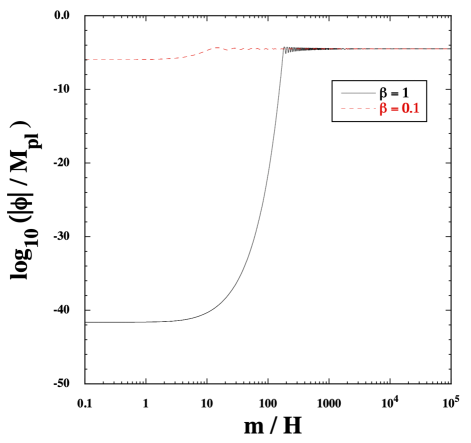
Figure 2: Evolution of $|\phi|/M_{\rm Pl}$ versus $m/H$ in the radiation-dominated epoch for $\beta=1,0.1$ with $m=1.0\times 10^{-11}$ eV and $f_{B}=1.0\times 10^{-5}M_{\rm Pl}$. The initial conditions of $\phi$ are chosen to match with those derived in the numerical simulations of Fig. 1 at the end of reheating.

In Fig. 2, we plot the evolution of $|\phi|/M_{\rm Pl}$ as a function of $m/H$ for $\beta=1,0.1$. We choose $m=10^{-11}$ eV and $f_{B}=1.0\times 10^{-5}M_{\rm Pl}$ with the initial conditions of $\phi$ consistent with their values at the end of reheating. For $\beta=1$, the field $\phi$ is nearly frozen with the value of order $10^{-42}M_{\rm Pl}$ and then starts to grow for $H\lesssim m/3$. Around $H\lesssim m/200$, the field sufficiently approaches the potential minimum and exhibits a damped oscillation around $\phi=\pi f_{B}$. When $\beta=0.1$, the field starts to evolve for $H\lesssim m/3$ as well, while the approach to $\phi=\pi f_{B}$ occurs around $H\lesssim m/12$ because of the large initial value of $\phi$ of order $10^{-6}M_{\rm Pl}$.

In the era dominated by the radiation density $\rho_{r}=\pi^{2}g_{*}T^{4}/30$, where $g_{*}$ is the number of relativistic degrees of freedom and $T$ is the temperature, we estimate the temperature $T_{m}$ at which the field $\phi$ starts to evolve along the potential $V(\phi)$. Using the Friedmann equation $3H^{2}M_{\rm Pl}^{2}=\rho_{r}$ with $m=3H$, it follows that

$$T_{m}=\left(\frac{10}{\pi^{2}g_{*}}\right)^{1/4}\sqrt{mM_{\rm Pl}}\,.$$ (33)

For the mass scale $m=10^{-11}$ eV with $g_{*}\simeq 10$ Dodelson (2003), we have $T_{m}\simeq 10^{12}$ K. Then, the field $\phi$ reaches the potential minimum $\pi f_{B}$ before the epoch of big-bang nucleosynthesis (BBN). After the Universe enters the matter-dominated epoch, the term $\dot{H}+2H^{2}$ in Eq. (16) is nonvanishing, i.e., $\dot{H}+2H^{2}\simeq H^{2}/2$. Since $m^{2}\gg H^{2}$ in this epoch, the effect of the nonminimal coupling on Eq. (16) is negligible and the field $\phi$ coherently oscillates around $\phi=\pi f_{B}$ with a decreasing amplitude. This is also the case for the late-time dark energy dominated era, so the field $\phi$ reaches the potential minimum by today.

III.2.2 Oscillation around the potential minimum as CDM

Around $\phi=\pi f_{B}$, the potential (10) is approximated as

$$V(\phi)\simeq\frac{1}{2}m^{2}(\phi-\pi f_{B})^{2}\,.$$ (34)

After the scalar field starts to oscillate about the potential minimum, it behaves as (a portion of) CDM with the energy density decreasing as $\rho_{\phi}\propto a^{-3}$. Today’s field density can be estimated as $\rho_{\phi 0}\simeq m^{2}f_{B}^{2}a_{\rm CDM}^{3}$, where $a_{\rm CDM}$ is the scale factor at which the field $\phi$ starts to behave as CDM during the radiation era and the scale factor is normalized as $a_{0}=1$. Defining the ratio

$$r_{\rm CDM}=\frac{m}{H_{\rm CDM}}$$ (35)

with $H_{\rm CDM}=H_{0}\sqrt{\Omega_{r0}a_{\rm CDM}^{-4}}$, where $H_{0}$ and $\Omega_{r0}$ are today’s Hubble parameter and radiation density parameter respectively, today’s field density parameter $\Omega_{\phi 0}=\rho_{\phi 0}/(3M_{\rm Pl}^{2}H_{0}^{2})$ can be estimated as

$$\Omega_{\phi 0}=\frac{r_{\rm CDM}^{3/2}}{3}\left(\frac{f_{B}}{M_{\rm Pl}}\right)^{2}\left(\frac{m}{H_{0}}\right)^{1/2}\Omega_{r0}^{3/4}\,.$$ (36)

If the field $\phi$ is responsible for a part of CDM, we require that $\Omega_{\phi 0}\simeq 0.27\alpha_{\rm CDM}$, where the constant $\alpha_{\rm CDM}$ represents the energy fraction of $\phi$ to CDM and $\alpha_{\rm CDM}=1$ corresponds to the case that $\phi$ is responsible for all CDM. Then, we obtain

$$\frac{f_{B}}{M_{\rm Pl}}\simeq 30r_{\rm CDM}^{-3/4}\sqrt{\alpha_{\rm CDM}}\left(\frac{m}{10^{-33}~{}{\rm eV}}\right)^{-1/4}\,,$$ (37)

where we used $\Omega_{r0}\simeq 9\times 10^{-5}$ and $H_{0}\simeq 10^{-33}$ eV. If $m=10^{-11}$ eV, then we have $f_{B}/M_{\rm Pl}\simeq 9.4\times 10^{-5}\sqrt{\alpha_{\rm CDM}}\,r_{\rm CDM}^{-3/4}$. Using the value $r_{\rm CDM}=200$ for $\beta=1$, we obtain $f_{B}/M_{\rm Pl}\simeq 2\times 10^{-6}\sqrt{\alpha_{\rm CDM}}$. For $\beta=0.1$ we take the value $r_{\rm CDM}=12$, in which case $f_{B}/M_{\rm Pl}\simeq 1\times 10^{-5}\sqrt{\alpha_{\rm CDM}}$. Under the constraint (37), the density parameter of $\phi$ at $a=a_{\rm CDM}$ (which is slightly before the BBN epoch) is as small as

$$\Omega_{\phi}(a=a_{\rm CDM})\simeq\frac{m^{2}f_{B}^{2}}{3M_{\rm Pl}^{2}H_{\rm CDM}^{2}}\simeq\frac{f_{B}^{2}}{3M_{\rm Pl}^{2}}r_{\rm CDM}^{2}\simeq 300r_{\rm CDM}^{1/2}\alpha_{\rm CDM}\left(\frac{m}{10^{-33}{\rm eV}}\right)^{-1/2}=3\times 10^{-9}r_{\rm CDM}^{1/2}\alpha_{\rm CDM}\,,$$ (38)

and hence the BBN is not affected by the presence of the field $\phi$.

The relation (37) has been derived by assuming that the scalar field $\phi$ behaves as a coherently oscillating CDM by today. If the energy density of $\phi$ decays to that of radiation or some other particle whose density decreases faster than radiation, then it is possible to have larger values of $f_{B}$ than those constrained by Eq. (37). For example, adding a decay term $\Gamma_{\phi}\dot{\phi}$ to the left hand-side of Eq. (16) leads to the dissipation of the energy density of $\phi$ before the field reaches the VEV $\phi_{v}=\pi f_{B}$. When we study scalarized NS solutions in Sec. V, we will allow for the possibility that $f_{B}/M_{\rm Pl}$ is larger than the value constrained by Eq. (37).

IV Weak gravitational objects

In this section, we study solutions of the scalar field $\phi$ for compact objects on weak gravitational backgrounds (like the Sun). For this purpose, we consider a static and spherically symmetric background given by the line element

$$\mathrm{d}s^{2}=g_{\mu\nu}{\rm d}x^{\mu}{\rm d}x^{\nu}=-f(r)\mathrm{d}t^{2}+h^{-1}(r)\mathrm{d}r^{2}+r^{2}\left(\mathrm{d}\theta^{2}+\sin^{2}\theta\,\mathrm{d}\varphi^{2}\right)\,,$$ (39)

where $f(r)$ and $h(r)$ are functions of the radial coordinate $r$. The scalar field is assumed to be a function of $r$ alone, i.e., $\phi=\phi(r)$. For the matter species inside a star, we consider a perfect fluid described by the mixed energy-momentum tensor $T^{\mu}{}_{\nu}={\rm diag}\left[-\rho(r),P(r),P(r),P(r)\right]$, where the energy density $\rho$ and pressure $P$ are functions of $r$. Assuming that the perfect fluid is minimally coupled to gravity, it obeys the continuity Eq. (6). On the background (39), this equation translates to

$$P^{\prime}+\frac{f^{\prime}}{2f}\left(\rho+P\right)=0\,,$$ (40)

where a ‘prime’ represents the derivative with respect to $r$.

Varying the action (1) with respect to $f$ and $h$, we obtain the following gravitational field equations

$$\frac{f^{\prime}}{f}=\frac{4(1-h)M_{\rm Pl}^{4}+2M_{\rm Pl}^{2}hr\phi^{\prime}(r\phi^{\prime}+4\beta\phi)-3\beta^{2}\phi^{2}\phi^{\prime 2}hr^{2}-4(V-P)r^{2}M_{\rm Pl}^{2}{\rm e}^{\beta\phi^{2}/(2M_{\rm Pl}^{2})}}{2M_{\rm Pl}^{2}hr(2M_{\rm Pl}^{2}-\beta\phi\phi^{\prime}r)}\,,$$ (41)

$$\frac{h^{\prime}}{h}-\frac{f^{\prime}}{f}=\frac{r[2M_{\rm Pl}^{2}\beta h\phi\phi^{\prime\prime}+\{2(\beta-1)M_{\rm Pl}^{2}+\beta^{2}\phi^{2}\}h\phi^{\prime 2}-2M_{\rm Pl}^{2}(\rho+P){\rm e}^{\beta\phi^{2}/(2M_{\rm Pl}^{2})}]}{M_{\rm Pl}^{2}h(2M_{\rm Pl}^{2}-\beta\phi\phi^{\prime}r)}\,.$$ (42)

The scalar field obeys the differential equation

$$\phi^{\prime\prime}+\frac{2(1+h)M_{\rm Pl}^{2}+\beta\phi^{\prime 2}hr^{2}-r^{2}(2V+\rho-P){\rm e}^{\beta\phi^{2}/(2M_{\rm Pl}^{2})}}{2M_{\rm Pl}^{2}hr}\phi^{\prime}$$

$$-\frac{(2M_{\rm Pl}^{2}-\beta\phi\phi^{\prime}r){\rm e}^{\beta\phi^{2}/(2M_{\rm Pl}^{2})}}{4M_{\rm Pl}^{4}h}\left[2V_{,\phi}M_{\rm Pl}^{2}+4\beta\phi V+\beta(\rho-3P)\phi\right]=0\,.$$ (43)

As we discussed in Sec. III, for $\beta>{\cal O}(0.1)$, the scalar field $\phi$ approaches the VEV $\phi_{v}=\pi f_{B}$ by today during the cosmic expansion history. We would like to construct a scalar-field profile $\phi(r)$ having the asymptotic value $\pi f_{B}$ at spatial infinity, i.e.,

$$\phi(\infty)=\pi f_{B}\,,$$ (44)

with $\phi^{\prime}(\infty)=0$. At $r=0$, we impose the boundary conditions $\phi(0)=\phi_{0}$ and $\phi^{\prime}(0)=0$, where $\phi_{0}$ is a constant in the range $0<\phi_{0}<\pi f_{B}$.

Since we are now considering a nonrelativistic object, we ignore $P$ relative to $\rho$ and employ the approximation $\rho r^{2}\ll M_{\rm Pl}^{2}$ inside the star. The gravitational potentials are much smaller than 1, so we can exploit the approximation $h\simeq 1$ in Eq. (43). As we will see below, the field variation $\phi^{\prime}(r)$ is small on weak gravitational backgrounds, under which $\beta\phi^{\prime 2}r^{2}\ll M_{\rm Pl}^{2}$ and $|\beta\phi\phi^{\prime}r|\ll M_{\rm Pl}^{2}$. In the vicinity of $\phi=\pi f_{B}$, the potential (10) can be also expanded as Eq. (34). Around $\phi=\pi f_{B}$, Eq. (43) is approximately given by

$$\phi^{\prime\prime}+\frac{2}{r}\phi^{\prime}-\left[m^{2}\left(\phi-\pi f_{B}\right)+\frac{\beta\rho}{2M_{\rm Pl}^{2}}\phi\right]\simeq 0\,.$$ (45)

By the end of this section, we consider a star with the constant density $\rho$ and radius $r_{s}$. We assume that the exterior region of the star has a vanishing density ($\rho=0$). Then, for $r>r_{s}$, the solution to Eq. (45) consistent with the boundary condition $\phi^{\prime}(\infty)=0$ is given by

$$\phi(r)=\pi f_{B}+\frac{A{\rm e}^{-mr}}{r}\,,$$ (46)

where $A$ is a constant.

Inside the star, the field Eq. (45) can be expressed as

$$\phi^{\prime\prime}+\frac{2}{r}\phi^{\prime}-\mu^{2}\left(\phi-\phi_{0}\right)=0\,,$$ (47)

where

$$\mu^{2}\equiv m^{2}+\frac{\beta\rho}{2M_{\rm Pl}^{2}}\,,\qquad\phi_{0}\equiv\frac{m^{2}}{\mu^{2}}\pi f_{B}\,.$$ (48)

For $\beta>0$, we have $\mu^{2}>m^{2}$ and hence $\phi_{0}<\pi f_{B}$. If we consider the Sun with the mean density $\rho={\cal O}(1~{}{\rm g/cm}^{3})$ and mass $m={\cal O}(10^{-11}\,{\rm eV})$, we have $m^{2}\gg\beta\rho/(2M_{\rm Pl}^{2})$, under which $\phi_{0}$ is very close to $\pi f_{B}$. Since we are assuming that $\rho={\rm constant}$, the solution to Eq. (47) consistent with the boundary condition $\phi^{\prime}(0)=0$ is given by

$$\phi(r)=\phi_{0}+\frac{B({\rm e}^{\mu r}-{\rm e}^{-\mu r})}{r}\,,$$ (49)

where $B$ is a constant.

Matching Eq. (46) with (49) and also their $r$ derivatives at $r=r_{s}$, we obtain

$$A=\frac{(\phi_{0}-\pi f_{B})[(\mu r_{s}-1)\,{\rm e}^{2\mu r_{s}}+\mu r_{s}+1]\,{\rm e}^{mr_{s}}}{(\mu+m)\,{\rm e}^{2\mu r_{s}}+\mu-m}\,,\qquad B=-\frac{(\phi_{0}-\pi f_{B})(mr_{s}+1)\,{\rm e}^{mr_{s}}}{(\mu+m)\,{\rm e}^{2\mu r_{s}}+\mu-m}\,.$$ (50)

Then, the resulting solution of $\phi$ outside the star ($r>r_{s}$) is given by

$$\phi(r)=\pi f_{B}-\beta_{\rm eff}M_{\rm Pl}\frac{GM_{g}}{r}{\rm e}^{-m(r-r_{s})}\,,$$ (51)

where $G=1/(8\pi M_{\rm Pl}^{2})$ is the gravitational constant, $M_{g}=4\pi r_{s}^{3}\rho/3$ is the mass of body, and

$$\beta_{\rm eff}=3\beta\frac{\pi f_{B}}{M_{\rm Pl}}\frac{(\mu r_{s}-1)\,{\rm e}^{2\mu r_{s}}+\mu r_{s}+1}{\mu^{2}r_{s}^{3}[(\mu+m)\,{\rm e}^{2\mu r_{s}}+\mu-m]}\,.$$ (52)

The fifth force between the scalar field and baryons is mediated by the effective coupling $\beta_{\rm eff}$. Note that the solution (51) looks similar to that derived in the chameleon mechanism Khoury and Weltman (2004a, b), but the difference is that the effective mass of $\phi$ inside and outside the star is similar to each other ($\mu\simeq m$) in our scenario. This leads to the different form of $\beta_{\rm eff}$ in comparison to the chameleon case.

If we consider the Sun ($r_{s}=7.0\times 10^{8}$ m) with the mass $m=10^{-11}$ eV, we have $\mu^{2}\simeq m^{2}\gg\beta\rho/(2M_{\rm Pl}^{2})$ and $\mu r_{s}\simeq mr_{s}\simeq 3.5\times 10^{4}$. In this case, Eq. (52) reduces to

$$\beta_{\rm eff}\simeq\frac{3\beta}{2}\frac{\pi f_{B}}{M_{\rm Pl}}\frac{1}{(mr_{s})^{2}}\qquad{\rm for}\quad mr_{s}\gg 1\,.$$ (53)

Because of a large suppression factor $(mr_{s})^{-2}$, it is easier to satisfy Solar-system constraints in comparison to the massless case (see below). For the symmetry-breaking scale $f_{B}/M_{\rm Pl}=2\times 10^{-6}$ with $\beta=1$, the effective coupling is as small as $\beta_{\rm eff}\simeq 7.7\times 10^{-15}$. In the case of Earth ($r_{s}=6.4\times 10^{6}$ m) with $m=10^{-11}$ eV, $f_{B}/M_{\rm Pl}=2\times 10^{-6}$, and $\beta=1$, we have $\beta_{\rm eff}\simeq 9.2\times 10^{-11}$. In addition to these small values of $\beta_{\rm eff}$, the factor ${\rm e}^{-m(r-r_{s})}$ in Eq. (51) leads to the exponential suppression of fifth forces at the distance $r\gtrsim r_{s}+1/m$.

In the massless limit $mr_{s}\to 0$, we have $\mu^{2}\simeq\beta\rho/(2M_{\rm Pl}^{2})$. Since $(\mu r_{s})^{2}$ is of order the gravitational potential at the surface of star, we exploit the approximation $\mu r_{s}\ll 1$ in Eq. (52). Then, the effective coupling reduces to

$$\beta_{\rm eff}\simeq\beta\frac{\pi f_{B}}{M_{\rm Pl}}\qquad{\rm for}\quad mr_{s}\to 0\,.$$ (54)

For $\beta$ of order 1, we have $\beta_{\rm eff}\ll 1$ under the condition $\pi f_{B}/M_{\rm Pl}\ll 1$, in which case it is possible to satisfy Solar-system constraints even for a nearly massless scalar field (as we will see at the end of this section).

Outside the star, we estimate fifth-force corrections to the metric components $f$ and $h$. They are related to the gravitational potentials $\Psi$ and $\Phi$, as $f={\rm e}^{2\Psi}$ and $h={\rm e}^{2\Phi}$. Since $|\Psi|$ and $|\Phi|$ are much smaller than 1 on weak gravitational backgrounds (of order $10^{-6}$ for the Sun), we only pick up terms linear in $\Psi$ and $\Phi$. Let us consider the massive scalar field satisfying the condition

$$mr_{s}\gg 1\,.$$ (55)

Substituting the solution (51) and its $r$ derivatives into Eqs. (41) and (42), we find that the gravitational potentials $\Phi$ and $\Psi$ approximately obey

$$\Phi^{\prime}+\frac{\Phi}{r}\simeq-\frac{1}{2}\beta\beta_{\rm eff}GM_{g}\frac{\pi f_{B}}{M_{\rm Pl}}m^{2}{\rm e}^{-m(r-r_{s})}\,,$$ (56)

$$\Psi^{\prime}+\frac{\Phi}{r}\simeq\beta\beta_{\rm eff}\frac{GM_{g}}{r}\frac{\pi f_{B}}{M_{\rm Pl}}m\,{\rm e}^{-m(r-r_{s})}\,.$$ (57)

The integrated solutions to these equations, which are consistent with the asymptotic flatness, are given by

$$\Phi = -\frac{GM_{g}}{r}\left[1-\frac{\beta\beta_{\rm eff}}{2}\frac{\pi f_{B}}{M_{\rm Pl}}mr\,{\rm e}^{-m(r-r_{s})}\right]\,,$$ (58)

$$\Psi = -\frac{GM_{g}}{r}\left[1+\frac{\beta\beta_{\rm eff}}{2}\frac{\pi f_{B}}{M_{\rm Pl}}{\rm e}^{-m(r-r_{s})}\right]\,.$$ (59)

We introduce the post-Newtonian parameter as

$$\gamma_{\rm PPN}\equiv\frac{\Phi}{\Psi}\simeq 1-\frac{\beta\beta_{\rm eff}}{2}\frac{\pi f_{B}}{M_{\rm Pl}}mr\,{\rm e}^{-m(r-r_{s})}\,.$$ (60)

The time-delay effect of the Cassini tracking of the Sun has given the bound $\gamma_{\rm PPN}-1=(2.1\pm 2.3)\times 10^{-5}$ Will (2014). Since $\gamma_{\rm PPN}-1$ is negative in the current theory, we adopt the limit $1-\gamma_{\rm PPN}\leq 2.0\times 10^{-6}$. Taking the value of $\gamma_{\rm PPN}$ at $r=r_{s}$, this Solar-system constraint translates to

$$\beta\beta_{\rm eff}\frac{\pi f_{B}}{M_{\rm Pl}}mr_{s}\leq 4.0\times 10^{-6}\,.$$ (61)

On using the effective coupling (53) derived for $mr_{s}\gg 1$, we obtain the bound

$$\beta\frac{\pi f_{B}}{M_{\rm Pl}}\frac{1}{\sqrt{mr_{s}}}\leq 1.6\times 10^{-3}\qquad{\rm for}\quad mr_{s}\gg 1\,.$$ (62)

With the mass scale $m=10^{-11}$ eV, this translates to $\pi f_{B}/M_{\rm Pl}\leq 0.3/\beta$ for the Sun. The symmetry-breaking scale $f_{B}/M_{\rm Pl}\simeq 2\times 10^{-6}$ with $\beta=1$, which was mentioned in Sec. III in the context of an oscillating $\phi$-field CDM, is well consistent with this upper limit.

We also comment on Solar-system constraints in the massless limit ($mr_{s}\to 0$). In this case, the scalar-field solution is given by Eq. (51) with $\beta_{\rm eff}=\beta\pi f_{B}/M_{\rm Pl}$. Provided that $\pi f_{B}/M_{\rm Pl}$ is smaller than the order 1, the gravitational potential $\Phi$ is estimated as $\Phi=-GM_{g}/r$ up to the linear order in $GM_{g}/r$, while the other gravitational potential receives a correction from the nonminimal coupling as $\Psi=-(GM_{g}/r)[1+\beta^{2}(\pi f_{B}/M_{\rm Pl})^{2}]$. Then, the post-Newtonian parameter is estimated as

$$\gamma_{\rm PPN}\simeq 1-\beta^{2}\left(\frac{\pi f_{B}}{M_{\rm Pl}}\right)^{2}\,,$$ (63)

where we used the approximation $\beta^{2}(\pi f_{B}/M_{\rm Pl})^{2}\ll 1$. Note that the result (63) is consistent with that derived in Ref. Damour and Esposito-Farese (1992). Using the Solar-system bound $1-\gamma_{\rm PPN}\leq 2.0\times 10^{-6}$, it follows that

$$\beta\frac{\pi f_{B}}{M_{\rm Pl}}\leq 1.4\times 10^{-3}\qquad{\rm for}\quad mr_{s}\to 0\,.$$ (64)

For the symmetry-breaking scale $f_{B}/M_{\rm Pl}\simeq 2\times 10^{-6}$ with $\beta=1$, the bound (64) is satisfied. In the massive case (62) there is an extra suppression factor $1/\sqrt{mr_{s}}\ll 1$, and the propagation of fifth forces is suppressed in comparison to the massless case.

For laboratory tests of gravity, the associated scale $r$ of experiments is in the range $mr\ll 1$. Let us consider two identical test bodies with constant density $\rho$, radius $r_{s}$, and mass $M_{g}=4\pi r_{s}^{3}\rho/3$. In this case, the gravitational potential $\Psi$ made by one test body is given by Eq. (59), with $\beta_{\rm eff}\simeq\beta\pi f_{B}/M_{\rm Pl}$ and ${\rm e}^{-m(r-r_{s})}\simeq 1$. Then, the potential energy between two test bodies is expressed as

$$V(r)=M_{g}\Psi=-\frac{GM_{g}^{2}}{r}\left[1+\frac{\beta^{2}}{2}\left(\frac{\pi f_{B}}{M_{\rm Pl}}\right)^{2}\right]\,.$$ (65)

The second term in the squared bracket of Eq. (65), which corresponds to the fifth-force contribution to $V(r)$, can be expressed in the form $\beta_{\rm eff}^{2}/2$. This result is analogous to what was obtained for chameleon and symmetron theories Khoury and Weltman (2004b); Sakstein (2018). Parametrizing the fifth-force potential energy as $V_{\rm f}(r)=-\alpha_{\rm f}GM_{g}^{2}/r$, the laboratory tests of gravity gives the constraint $\alpha_{\rm f}<10^{-3}$ Adelberger et al. (2009). Since $\alpha_{\rm f}=(\beta^{2}/2)(\pi f_{B}/M_{\rm Pl})^{2}$ in our case, we obtain the following bound

$$\beta\frac{\pi f_{B}}{M_{\rm Pl}}\leq 4.5\times 10^{-2}\,.$$ (66)

This is weaker than the Solar-system constraint (64) by one order of magnitude. On astrophysical scales much larger than $m^{-1}={\cal O}(10\,{\rm km})$, our model is consistent with observational tests of gravity due to the exponential suppression of fifth forces.

For the choice $m^{-1}={\cal O}(10\,{\rm km})$, we may also apply the experimental tests of Newton’s law on geophysical scales to our model. Assuming that the Yukawa-type corrections to the Newtonian potential $V_{g}(r)=-(GM_{g}/r)\left(1+\alpha_{\rm f}e^{-r/\lambda}\right)$ for the scale $\lambda={\cal O}(10\,{\rm km})$, the bound on $\alpha_{\rm f}$ is given by $|\alpha_{\rm f}|\lesssim 10^{-4}$ (see e.g., Fig. 4 of Ref. Adelberger et al. (2003)). Comparing $V_{g}(r)$ with Eq. (59), we find

$$\beta\beta_{\rm eff}\frac{\pi f_{B}}{M_{\rm Pl}}\lesssim 10^{-4}\,.$$ (67)

This is weaker than the Solar System bound (61) derived for $mr_{s}\gg 1$.

V Neutron star solutions

In this section, we will construct NS solutions on the static and spherically symmetric background given by the line element (39). We note that Eqs. (40)-(43) are the strict Euler-Lagrange equations obtained by varying the action (1) and hence valid also on strong gravitational backgrounds. The difference from the case of weak gravitational stars discussed in Sec. IV is that the gravitational potentials $|\Psi|$ and $|\Phi|$ in the vicinity of NSs are of ${\cal O}(0.1)$ and nonlinearities in the gravitational field equations become important. Moreover, the pressure $P$ is not negligible relative to the energy density $\rho$. The other important difference is that the central density of NSs $\rho_{c}$ is typically of ${\cal O}(10^{15}~{}{\rm g/cm}^{3})$, so in our model the term $\beta\rho/(2M_{\rm Pl}^{2})$ can exceed $m^{2}={\cal O}\left((10^{-11}~{}{\rm eV})^{2}\right)$ for $\beta\gtrsim{\cal O}(0.1)$. This means that the field value $\phi_{0}$ defined in Eq. (48) can approach 0 inside the NS, unlike the low density star where $\phi_{0}$ is very close to $\pi f_{B}$. Then, it should be possible to realize a scalar-field configuration in which $\phi$ is close to $\phi=0$ inside the star and approaches $\pi f_{B}$ outside the star. In the following, we will show that such scalarized solutions do exist.

V.1 Boundary conditions

We first derive the approximate solutions around the center of star by using the expansions of $f$, $h$, $\phi$, and $P$. Due to the regularity condition $\phi^{\prime}(0)=0$, we can expand the scalar field around $r=0$ in the form $\phi(r)=\phi_{c}+\phi_{2}r^{2}+{\cal O}(r^{3})$, where $\phi_{c}=\phi(0)$ and $\phi_{2}$ is a constant. We also impose the boundary conditions $f(0)=f_{c}$, $h(0)=1$, $\rho(0)=\rho_{c}$, $P(0)=P_{c}$, and $f^{\prime}(0)=h^{\prime}(0)=\rho^{\prime}(0)=P^{\prime}(0)=0$. Around $r=0$, the scalar-field potential is expanded as

$$V(\phi)=V_{c}+V_{,\phi c}(\phi-\phi_{c})+{\cal O}((\phi-\phi_{c})^{2})\,,$$ (68)

where we used the notations $V_{c}\equiv V(\phi_{c})$ and $V_{,\phi c}\equiv(\mathrm{d}V/\mathrm{d}\phi)(\phi_{c})$. The solutions consistent with Eqs. (40)-(43) around the center of NSs are given by

$$f = f_{c}+f_{c}\frac{{\rm e}^{\beta\phi_{c}^{2}/(2M_{\rm Pl}^{2})}[2(\rho_{c}+3P_{c}-2V_{c})M_{\rm Pl}^{2}+2\beta\phi_{c}M_{\rm Pl}^{2}V_{,\phi c}+\beta^{2}\phi_{c}^{2}(\rho_{c}-3P_{c}+4V_{c})]}{12M_{\rm Pl}^{4}}r^{2}+{\cal O}(r^{4})\,,$$ (69)

$$h = 1-\frac{{\rm e}^{\beta\phi_{c}^{2}/(2M_{\rm Pl}^{2})}[2(\rho_{c}+V_{c})M_{\rm Pl}^{2}-2\beta\phi_{c}M_{\rm Pl}^{2}V_{,\phi c}-\beta^{2}\phi_{c}^{2}(\rho_{c}-3P_{c}+4V_{c})]}{6M_{\rm Pl}^{4}}r^{2}+{\cal O}(r^{4})\,,$$ (70)

$$\phi = \phi_{c}+\frac{{\rm e}^{\beta\phi_{c}^{2}/(2M_{\rm Pl}^{2})}}{6}\left[V_{,\phi c}+\frac{\beta\phi_{c}(\rho_{c}-3P_{c}+4V_{c})}{2M_{\rm Pl}^{2}}\right]r^{2}+{\cal O}(r^{4})\,,$$ (71)

$$P = P_{c}-\frac{{\rm e}^{\beta\phi_{c}^{2}/(2M_{\rm Pl}^{2})}(\rho_{c}+P_{c})[2(\rho_{c}+3P_{c}-2V_{c})M_{\rm Pl}^{2}+2\beta\phi_{c}M_{\rm Pl}^{2}V_{,\phi c}+\beta^{2}\phi_{c}^{2}(\rho_{c}-3P_{c}+4V_{c})]}{24M_{\rm Pl}^{4}}r^{2}+{\cal O}(r^{4})\,.$$ (72)

Let us consider the case in which $\phi_{c}$ is in the range $0<\phi_{c}\ll\pi f_{B}$. The potential energy around $\phi=0$ is of order $V\simeq 2m^{2}f_{B}^{2}$, with $V_{,\phi}\simeq-m^{2}\phi$. Provided that $f_{B}\ll M_{\rm Pl}$, it follows that $V$ is much smaller than the central density $\rho_{c}={\cal O}(10^{15}\,{\rm g/cm}^{3})$ for $m={\cal O}(10^{-11}$ eV). Then, the solution (71) is approximately given by

$$\phi\simeq\phi_{c}+\frac{{\rm e}^{\beta\phi_{c}^{2}/(2M_{\rm Pl}^{2})}}{6}\phi_{c}m_{\rm eff}^{2}r^{2}+{\cal O}(r^{3})\,,$$ (73)

where

$$m_{\rm eff}^{2}\equiv-m^{2}+\frac{\beta\rho_{c}(1-3w_{c})}{2M_{\rm Pl}^{2}}\,,$$ (74)

with the equation of state (EOS) parameter $w_{c}=P_{c}/\rho_{c}$ at $r=0$. Here, $m_{\rm eff}^{2}$ corresponds to an effective mass squared of the scalar field around the potential maximum at $\phi=0$. Like Eq. (11), for $\beta=0$, we have $m_{\rm eff}^{2}=-m^{2}<0$, so the scalar field decreases as a function of $r$, i.e., $\phi^{\prime}(r)<0$, around $r=0$. In the presence of the positive nonminimal coupling $\beta$ with $w_{c}<1/3$, it is possible to realize $m_{\rm eff}^{2}>0$ for

$$\beta>\frac{2m^{2}M_{\rm Pl}^{2}}{\rho_{c}(1-3w_{c})}=\frac{0.28}{1-3w_{c}}\left(\frac{10^{15}~{}{\rm g/cm}^{3}}{\rho_{c}}\right)\left(\frac{m}{10^{-11}~{}{\rm eV}}\right)^{2}\,,$$ (75)

where the right hand-side is equivalent to the critical value $\beta_{c}$ given in Eq. (12). For large values of $\rho_{c}$, $w_{c}$ can be close to the relativistic value $1/3$ or even larger, so we need to implement the pressure to derive the scalar-field profile correctly. For $w_{c}<1/3$ the scalar field increases as a function of $\phi$ around $r=0$, so it is possible to reach the asymptotic value $\phi_{v}=\pi f_{B}$ at spatial infinity. Even if $\phi(r)$ decreases around $r=0$ for $w_{c}>1/3$, the decrease of the EOS parameter $w=P/\rho$ around the NS surface to the region $w<1/3$ allows a possibility for increasing $\phi(r)$ to reach $\phi_{v}=\pi f_{B}$ outside the star. We note that we have ignored the term $4V_{c}$ in Eq. (71) relative to $\rho_{c}-3P_{c}$, but if $f_{B}$ is as close as the order $M_{\rm Pl}$, there is the contribution of the potential to $m_{\rm eff}^{2}$ especially around $w_{c}\simeq 1/3$.

In the asymptotic region outside the NSs, the field $\phi$ should relax toward the value $\pi f_{B}$. In this regime, we can set $\rho=P=0$, $V\to 0$, and $h\to 1$ in Eq. (43) and ignore the terms $\beta\phi^{\prime 2}r^{2}$ and $\beta\phi\phi^{\prime}r$ relative to $M_{\rm Pl}^{2}$. Keeping the term $V_{,\phi}\simeq m^{2}(\phi-\pi f_{B})$ around $\phi=\pi f_{B}$, the solution to Eq. (43) is approximately given by Eq. (46), but the coefficient $A$ is different from that on weak gravitational backgrounds.

V.2 Numerically constructed scalar-field profile

To study the existence of the field profile connecting the solution (73) to the other solution (46), we numerically integrate Eqs. (40)-(43) from the center of NSs to a sufficiently large distance. We exploit Eqs. (69)-(72) as the boundary conditions around $r=0$. In Eq. (69), we can set $f_{c}=1$ without loss of generality. The field value $\phi_{c}$ at the center of star is iteratively found from the demand of realizing the asymptotic value $\phi(r)\to\pi f_{B}$ with $\phi^{\prime}(r)\to 0$ far outside the star. For the perfect fluid inside the NS, we use the analytic representation of SLy EOS parametrized by

$$\xi=\log_{10}(\rho/{\rm g\cdot cm}^{-3})\,,\qquad\zeta=\log_{10}(P/{\rm dyn\cdot cm}^{-2})\,,$$ (76)

where the explicit relation between $\xi$ and $\zeta$ is given in Ref. Haensel and Potekhin (2004). The outside of NS is assumed to be in a vacuum with a vanishing density and pressure. For the numerical purpose, we introduce the following constants

$$\rho_{0}=m_{n}n_{0}=1.6749\times 10^{14}~{}{\rm g}/{\rm cm}^{3}\,,\qquad r_{0}=\sqrt{\frac{8\pi M_{\rm Pl}^{2}}{\rho_{0}}}=89.664~{}{\rm km}\,,$$ (77)

where $m_{n}=1.6749\times 10^{-24}$ g is the neutron mass and $n_{0}=0.1~{}(\rm fm)^{-3}$ is the typical number density of NSs. The density $\rho$ and radius $r$ are normalized by $\rho_{0}$ and $r_{0}$, respectively.

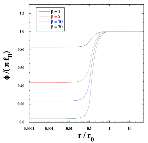
Figure 3: The scalar field $\phi$ (normalized by $\pi f_{B}$) versus the radius $r$ (normalized by the distance $r_{0}=89.664$ km) for $m=1.0\times 10^{-11}$ eV and $f_{B}=0.3M_{\rm Pl}/(\pi\beta)$. Each case corresponds to $\beta=1,5,10,30$. We choose the SLy EOS with the central density $\rho_{c}=6\rho_{0}$, where $\rho_{0}=1.6749\times 10^{14}~{}{\rm g/cm}^{3}$.

In Fig. 3, we plot $\phi/(\pi f_{B})$ versus $r/r_{0}$ for $\beta=1,5,10,30$ with the model parameters $m=1.0\times 10^{-11}$ eV and $f_{B}=0.3M_{\rm Pl}/(\pi\beta)$. The central density of NS is chosen to be $\rho_{c}=6\rho_{0}\simeq 10^{15}~{}{\rm g/cm}^{3}$. With this mass scale $m$ the local gravity constraint (62) gives the bound $\beta\pi f_{B}/M_{\rm Pl}\leq 0.3$ for the Sun, so the choice $f_{B}=0.3M_{\rm Pl}/(\pi\beta)$ corresponds to a maximally allowed value of $f_{B}$. When $\rho_{c}=6\rho_{0}$ the EOS parameter at $r=0$ is $w_{c}\simeq 0.158$, the condition (75) translates to $\beta>0.53$. In this case the effective mass squared $m_{\rm eff}^{2}$ is positive at $r=0$, and the scalar field grows according to Eq. (73) in the vicinity of $r=0$.

For $\beta=1$, the field value at $r=0$ is $\phi_{c}\simeq 0.83\pi f_{B}$, and the difference from the asymptotic value is $\pi f_{B}-\phi_{c}\simeq 0.17\pi f_{B}$. On weak gravitational backgrounds discussed in Sec. IV, the field values inside and outside a star are very close to each other, see Eq. (48) together with the condition $m^{2}\gg\beta\rho/(2M_{\rm Pl}^{2})$. Since the nonminimal coupling $\beta\rho/(2M_{\rm Pl}^{2})$ can be larger than $m^{2}$ for NSs around $r=0$, the difference between $\pi f_{B}$ and $\phi_{c}$ exceeds the order of $0.1\pi f_{B}$. With the increase of $\beta$, this difference tends to be more significant, e.g., $\phi_{c}\simeq 0.04\pi f_{B}$ for $\beta=30$. We note that the symmetry-breaking scale $f_{B}$ does not appear in the effective mass squared (74) at $r=0$. Hence the normalized field configuration $\phi/(\pi f_{B})$ is hardly sensitive to the change of $f_{B}$.

The large variation of $\phi(r)$ spanning in the range $0<\pi f_{B}-\phi_{c}\lesssim 0.1\pi f_{B}$ is an outcome of the positive mass squared $m_{\rm eff}^{2}$ induced by large values of $\rho_{c}$. Then, the scalar field acquires a sufficient kinetic energy around $r=0$ to reach the asymptotic value $\phi_{v}=\pi f_{B}$ far outside the NSs. This is not the case for weak gravitational objects where $\phi$ needs to stay around $\pi f_{B}$ both inside and outside the star. Thus, our model allows the existence of an interesting scalar-field profile whose variation is significant for strongly gravitating objects, while the variation of $\phi(r)$ is suppressed on weak gravitational backgrounds as consistent with Solar-system constraints.

V.3 Modification of gravitational interactions

The scalar-field profile derived above affects the nonlinearly extended gravitational potentials $\Psi$ and $\Phi$ through Eqs. (41) and (42). Since $f={\rm e}^{2\Psi}$ and $h={\rm e}^{2\Phi}$, the left hand-side of Eq. (42) is equivalent to $2(\Phi^{\prime}-\Psi^{\prime})$. In GR the right hand-side of Eq. (42) vanishes for $r\geq r_{s}$, where $r_{s}$ is the radial position of the NS radius. In the current model, however, there are contributions of $\phi(r)$ and its derivatives to the right hand-side of Eq. (42). To quantify the difference between $\Phi^{\prime}$ and $\Psi^{\prime}$, we define

$$\eta(r)\equiv\frac{\Phi^{\prime}(r)}{\Psi^{\prime}(r)}-1\,,$$ (78)

and compute it at the surface of star.

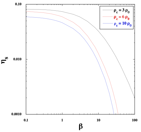
Figure 4: We show $\eta_{s}=\Phi^{\prime}(r_{s})/\Psi^{\prime}(r_{s})-1$ versus the nonminimal coupling $\beta$ for $m=1.0\times 10^{-11}$ eV and $f_{B}=0.3M_{\rm Pl}/(\pi\beta)$. We choose the SLy EOS with three different central densities $\rho_{c}=3\rho_{0},6\rho_{0},10\rho_{0}$.

In Fig. 4, we plot $\eta_{s}=\eta(r_{s})$ versus $\beta$ for $\rho_{c}=3\rho_{0},6\rho_{0},10\rho_{0}$ with $m=1.0\times 10^{-11}$ eV and $f_{B}=0.3M_{\rm Pl}/(\pi\beta)$. When $\rho_{c}=3\rho_{0}$, the quantity $\eta_{s}$ can be as large as $0.08$ for $\beta$ in the range 0.1$\sim$1. Since we are choosing the maximally allowed value of $f_{B}$ consistent with Solar-system constraints, increasing $\beta$ results in smaller values of $f_{B}$. Given that $\phi(r)$ is normalized by $\pi f_{B}$ in the numerical simulation of Fig. 3, decreasing $f_{B}$ implies smaller values of $\phi(r)$ inside the star. Then, as $\beta$ increases, the corrections to gravitational potentials induced by the nonvanishing field profile should be more suppressed. Indeed, for given $\rho_{c}$, the property of decreasing $\eta_{s}$ as a function of $\beta$ can be confirmed in Fig. 4.

As $\rho_{c}$ increases in the range $\rho_{c}\geq 2\rho_{0}$, $\eta_{s}$ decreases from the maximum around $(\eta_{s})_{\rm max}=0.08$ realized for the density $\rho_{c}=2\rho_{0}\sim 3\rho_{0}$. One of the reasons for this decrease of $\eta_{s}$ is that, for larger $\rho_{c}$, $w_{c}$ tends to increase. For $\rho_{c}=3\rho_{0},6\rho_{0},10\rho_{0}$, we have $w_{c}=0.047,0.158,0.315$, respectively. This means that, for $\rho_{c}\gtrsim 6\rho_{0}$, the product $\rho_{c}(1-3w_{c})$, which appears in the effective mass squared (74), gets smaller as $\rho_{c}$ increases. The other reason is that, as $\rho_{c}$ increases in the range $2\rho_{0}\leq\rho_{c}\lesssim 6\rho_{0}$, the field value $\phi_{c}$ at $r=0$ tends to be smaller by approaching the symmetry-restored state. This leads to the overall decrease of corrections of the scalar field $\phi$ to the right hand-sides of Eqs. (41) and (42). Due to these two combined effects, for increasing $\rho_{c}$ in the range $2\rho_{0}\leq\rho_{c}\lesssim 10\rho_{0}$, there is the tendency that $\eta_{s}$ decreases. Nevertheless, the observations of gravitational waves will provide us with interesting possibilities for probing the deviation from GR of order $\eta_{s}>{\cal O}(0.01)$ in the coupling range $\beta=0.1\sim 10$.

As $\rho_{c}$ exceeds $10\rho_{0}$, the product $\rho_{c}(1-3w_{c})$ can be negative. In such cases the EOS parameter $w=P/\rho$ decreases toward the NS surface, and there is a point at which $\rho(1-3w)$ becomes positive. Then, it is possible to have nontrivial scalar-field profiles even for $\rho_{c}(1-3w_{c})<0$, but the difference between $\pi f_{B}$ and $\phi_{c}$ tends to be smaller. For $\rho_{c}\gtrsim 10\rho_{0}$, this results in suppressed values of $\eta_{s}$ in comparison to the case $\rho_{c}\lesssim 10\rho_{0}$.

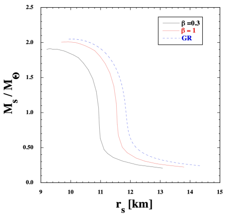
Figure 5: The ADM mass $M_{s}$ normalized by the Solar-mass $M_{\odot}$ versus the NS radius $r_{s}$ for the SLy EOS with $m=1.0\times 10^{-11}$ eV and $f_{B}=0.3M_{\rm Pl}/(\pi\beta)$. The solid black and red lines correspond to $\beta=0.3$ and $\beta=1$, respectively, while the dashed blue line is the case in GR. In all cases, the matter density at $r=0$ are in the range $2\rho_{0}\leq\rho_{c}\leq 18\rho_{0}$.

The ADM mass of NSs is defined by

$$M_{s}\equiv 4\pi M_{\rm Pl}^{2}r\left[1-h(r)\right]|_{r=\infty}\,,$$ (79)

while the NS radius is determined by the condition $P(r_{s})=0$. In Fig. 5, we plot the relation between $M/M_{\odot}$ and $r_{s}$ for $\beta=0.3$ and 1 with $m=1.0\times 10^{-11}$ eV and $f_{B}=0.3M_{\rm Pl}/(\pi\beta)$, where $M_{\odot}$ is the Solar mass. In comparison, we also show the case of GR derived for the SLy EOS without the scalar field $\phi$. The matter density $\rho_{c}$ at $r=0$ is chosen to be in the range $\rho_{c}\geq 2\rho_{0}$, under which the NS in GR has the ADM mass $M_{s}\geq 0.243M_{\odot}$ and radius $r_{s}\leq 14.33$ km.

In Fig. 5, we observe that, for $\beta>0$, both $M_{s}$ and $r_{s}$ are smaller than those in GR. For $\beta={\cal O}(0.1)$ the field value $\phi_{c}$ is generally quite close to $\pi f_{B}$, so the exponential factor ${\rm e}^{\beta\phi_{c}^{2}/(2M_{\rm Pl}^{2})}$ in Eq. (72) can be estimated as ${\rm e}^{\beta\phi_{c}^{2}/(2M_{\rm Pl}^{2})}\simeq 1+0.045/\beta>1$. This leads to the larger decreasing rate of $P(r)$ in comparison to GR, and hence $r_{s}$ and $M_{s}$ are reduced. Such reductions of $r_{s}$ and $M_{s}$ are different from the properties in standard spontaneous scalarization induced by the negative coupling $\beta$ Damour and Esposito-Farese (1993); Minamitsuji and Silva (2016); Doneva and Yazadjiev (2018b). For $\beta=0.3$ and $\rho_{c}=2\rho_{0}$ we obtain $r_{s}=13.08$ km and $M_{s}=0.207M_{\odot}$, so the relative difference from the ADM mass in GR ($M_{\rm GR}=0.243M_{\odot}$) with the same value of $\rho_{c}$ is as large as $\mu_{M}=0.15$, where we have defined

$$\mu_{M}\equiv 1-\frac{M_{s}}{M_{\rm GR}}.$$ (80)

As $\rho_{c}$ increases, the deviation parameter $\mu_{M}$ tends to decrease, e.g., $\mu_{M}=0.10$ for $\rho_{c}=5\rho_{0}$ and $\mu_{M}=0.07$ for $\rho_{c}=15\rho_{0}$. However, it is interesting to note that, for $\beta=0.3$, the difference of order 7 % from GR arises for the ADM mass even with high densities like $\rho_{c}\gtrsim 10\rho_{0}$.

With the increase of $\beta$, $\phi_{c}$ tends to decrease toward the symmetry-restored state $\phi=0$ and hence the exponential factor ${\rm e}^{\beta\phi_{c}^{2}/(2M_{\rm Pl}^{2})}$ approaches 1. Moreover, as we already discussed in Fig. 4, the quantity $\eta_{s}$ is a decreasing function of $\beta$ for the choice $f_{B}=0.3M_{\rm Pl}/(\pi\beta)$. Indeed, as we see the case $\beta=1$ in Fig. 5, the deviations of $M_{s}$ and $r_{s}$ from those in GR are less significant relative to the coupling $\beta=0.3$. Still, for $\beta=1$, we have $\mu_{M}=0.08$ for $\rho_{c}=2\rho_{0}$ and $\mu_{M}=0.04$ for $\rho_{c}=5\rho_{0}$, so the appreciable deviation from GR is present. For $\beta$ exceeding the order of 1, the theoretical curve in the $(M_{s},r_{s})$ plane approaches that of GR.

In standard spontaneous scalarization induced by negative values of $\beta$, the theoretical curve in the $(M_{s},r_{s})$ plane starts to be bifurcated from the GR one for $\rho_{c}$ larger than some critical density, and the mass of NSs in the scalarized branch are larger than that in GR with the same central density. This characterizes a continuous phase transition from the GR branch $\phi=0$ to the other nontrivial branch $\phi\neq 0$ triggered by a tachyonic instability. In our case, the scalarized NS solutions arise from the symmetry restored state at $\phi=0$ induced by positive $\beta$. Theoretical plots for $\beta>0$ differ from the GR curve in the whole range of $\rho_{c}$ shown in Fig. 5, i.e., $2\rho_{0}\leq\rho_{c}\leq 18\rho_{0}$. This is because in our model there is no GR solution and hence no bifurcation from it. Instead, we have only one branch of NS solutions where the scalar field $\phi$ asymptotically approaches the ground state located around $\phi=\pi f_{B}$.

In theories given by the action (1), the conditions for the absence of ghost/Laplacian instabilities against odd- and even-parity perturbations are given by $\rho+P>0$ and $F(\phi)>0$ Kase and Tsujikawa (2022) (see also Ref. Kase et al. (2020b)). Since we are considering the nonminimal coupling $F(\phi)={\rm e}^{-\beta\phi^{2}/(2M_{\rm pl}^{2})}$ with $\beta>0$ in the presence of a perfect-fluid matter satisfying the weak energy condition, there are neither ghost nor Laplacian instabilities for our scalarized NS solutions as in the case of standard spontaneous scalarization.

It should be noted that NSs in GR with other EOMs may provide the similar ADM mass and radius to those derived for nonzero $\beta$ in Fig. 5. In our case, since the mass of NSs is relatively suppressed to that in the GR case, it would be difficult to distinguish NSs in our theory from those in GR with a different choice of EOSs, only with observations regarding the mass and radius of NSs. In order to break the degeneracy between the modified gravity effects and the ambiguity associated with the choice of EOSs, we should explore the existence of universal relations which are almost insensitive to the choice of EOSs Yagi and Yunes (2013); Yagi et al. (2014); Breu and Rezzolla (2016) as well as signatures associated with gravitational perturbations of NSs such as tidal deformability and quasinormal frequencies. We leave these subjects for future works.

Finally, we should comment on the case in which the energy density of an oscillating scalar field $\phi$ around $\phi=\pi f_{B}$ is responsible for a fraction of CDM without decaying to other particles by today. In this case, the symmetry-breaking scale $f_{B}$ is constrained as Eq. (37). When $\beta=1$, this gives the constraint $f_{B}/M_{\rm Pl}\simeq 2\times 10^{-6}$. For such small values of $f_{B}$, the field $\phi$ inside and outside the NS is also suppressed and hence $\eta_{s}$ is at most of order $10^{-9}$ with the nonminimal coupling in the range $\beta\leq{\cal O}(10)$. In such cases, the NS mass and radius are also very similar to those in GR. However, there is a possibility that the oscillating field $\phi$ decays to other particles whose energy densities decrease as that of radiation or faster, in which case larger values of $f_{B}$ are allowed. In Figs. 4 and 5, we have used the maximum allowed values of $f_{B}$ consistent with Solar-system constraints.

VI Conclusions

We proposed a new scenario of NS scalarizations in the presence of a pNGB potential $V(\phi)=m^{2}f_{B}^{2}[1+\cos(\phi/f_{B})]$ and a nonminimal coupling to the Ricci scalar $R$ of the form $F(\phi)={\rm e}^{-\beta\phi^{2}/(2M_{\rm Pl}^{2})}$. In regions of the high density, the scalar field $\phi$ acquires a large positive mass squared by the nonminimal coupling with $\beta>0$. This can overwhelm a negative mass squared $-m^{2}$ of the bare potential at $\phi=0$. Then, the symmetry restoration toward $\phi=0$ occurs in strong gravitational backgrounds like the interior of NSs, while the scalar approaches a VEV $\phi_{v}=\pi f_{B}$ toward spatial infinity. This allows the existence of nontrivial field profiles affecting gravitational interactions in the vicinity of NSs.

Unlike the original scenario of spontaneous scalarization induced by negative $\beta$ with $V(\phi)=0$ Damour and Esposito-Farese (1993), our model does not suffer from the tachyonic instability of cosmological solutions. In Sec. III we studied the cosmological evolution of $\phi$ for $m={\cal O}(10^{-11}$ eV) and $f_{B}\lesssim M_{\rm Pl}$ relevant to the mass scales of NS scalarizations. For $\beta>{\cal O}(0.1)$, the amplitude of $\phi$ exponentially decreases during inflation due to the dominance of the positive nonminimal coupling over the tachyonic mass squared $-m^{2}$ in the effective mass squared $m_{\rm eff}^{2}$. During the reheating stage, the field amplitude exhibits mild decrease further. During the radiation-dominated era, after the contribution from the nonminimal coupling to $m_{\rm eff}^{2}$ drops below $-m^{2}$, $\phi$ starts to roll down the potential toward the VEV $\pi f_{B}$. Numerically, we showed that the scalar field starts to oscillate around $\phi=\pi f_{B}$ before the epoch of BBN. If the oscillation of $\phi$ has continued by today, it can be the source of (a portion of) CDM for $f_{B}$ satisfying Eq. (37). This relation is not applied to the case in which the energy density of oscillating $\phi$ is converted to other particles by today.

In Sec. IV, we derived the field profile for nonrelativistic stars with constant $\rho$ on weak gravitational backgrounds. Outside the star, the scalar field is given by Eq. (51) with the effective coupling (52). For the mass satisfying the condition $mr_{s}\gg 1$, where $r_{s}$ is the radius at the surface of star, the field stays in the region very close to $\phi=\pi f_{B}$. In this case, the gravitational potentials $\Phi$ and $\Psi$ receive fifth-force corrections as Eqs. (58) and (59). From Solar-system constraints on the post-Newtonian parameter $\gamma_{\rm PPN}=\Phi/\Psi$, we obtained the upper limit (62) on the product $\beta f_{B}$. With the mass scale $m=10^{-11}$ eV, the bound (62) translates to $\beta\pi f_{B}/M_{\rm Pl}\leq 0.3$ for the Sun. This is weaker than the constraint (64) derived in the massless limit $mr_{s}\to 0$ by two orders of magnitude.

In Sec. V, we have numerically constructed NS solutions in the presence of a positive nonminimal coupling with the self-interacting potential. We showed the existence of scalar-field profiles with significant difference between the field value $\phi_{c}$ at $r=0$ and the asymptotic value $\pi f_{B}$ at spatial infinity for static and spherically symmetric NSs. This is an outcome of the symmetry restoration toward $\phi=0$ in regions of the high density induced by the positive nonminimal coupling $\beta$. As we observe in Fig. 3, for larger $\beta$, the difference between $\phi_{c}$ and $\pi f_{B}$ tends to be more significant. The nonminimally coupled scalar field gives rise to modifications to the gravitational potentials $\Phi$ and $\Psi$ in comparison to GR. We computed the quantity $\eta_{s}=\Phi^{\prime}(r_{s})/\Psi^{\prime}(r_{s})-1$ by varying the central density $\rho_{c}$ in the range $\rho_{c}\geq 2\rho_{0}$. Taking the upper limit $f_{B}=0.3M_{\rm Pl}/(\pi\beta)$ constrained from Solar-system tests of gravity, we find that $\eta_{s}$ is a decreasing function of $\beta$ for given $\rho_{c}$. The increase of $\beta$ results in the decreases of $f_{B}$ and $\phi(r)$ inside the star, so the parameter $\eta_{s}$ tends to be suppressed. As $\rho_{c}$ increases, $\eta_{s}$ is also subject to the decrease due to several combined effects explained in the main text. Still, $\eta_{s}$ can be of order $\eta_{s}>{\cal O}(0.01)$ in the coupling range $\beta=0.1\sim 10$.

In Fig. 5, we plotted the relation between the ADM mass $M_{s}$ and the radius $r_{s}$ of NSs for $\beta=0.3$ and $\beta=1$ with $f_{B}=0.3M_{\rm Pl}/(\pi\beta)$. Unlike standard spontaneous scalarization, the deviation of $M_{s}$ and $r_{s}$ from their values in GR occurs for any central density in the range $2\rho_{0}\leq\rho_{c}\leq 18\rho_{0}$. For $\beta=0.3$, the relative difference of the ADM mass from that in GR, which is defined by $\mu_{M}=1-M_{s}/M_{\rm GR}$, is as large as $\mu_{M}=0.15$ for $\rho_{c}=2\rho_{0}$. As $\rho_{c}$ increases, $\mu_{M}$ tends to decrease, but $\mu_{M}$ still has a considerably large value $0.07$ even for $\rho_{c}=15\rho_{0}$. With the increase of $\beta$, the theoretical lines in the $(M_{s},r_{s})$ plane, which exist in the region $M_{s}<M_{\rm GR}$, approach that in GR. For $\beta=1$ and $\rho_{c}=2\rho_{0}$, we found that $\mu_{M}=0.08$ and hence there is still appreciable deviation from GR.

In summary, we showed that our new model of scalarizations of NSs associated with the symmetry restoration induced by the nonminimal coupling leads to modified gravitational interactions in the vicinity of NSs, while it is free from the problem of instabilities during the cosmological evolution. The implication of our model to observations of the binary NS coalescense was recently studied in Ref. Higashino and Tsujikawa (2023). Since the scalar field mass $m={\cal O}(10^{-11}\,{\rm eV})$ is larger than the typical orbital frequency of NS binaries $\omega={\cal O}(10^{-13}\,{\rm eV})$, the scalar radiation emitted from compact binaries during the inspiral phase is strongly suppressed. The resulting gravitational wave forms are similar to those in GR, so our model evades current observational constraints of inspiral gravitational wave forms.

References

- Abbott et al. (2016) B. P. Abbott et al. (LIGO Scientific, Virgo), Phys. Rev. Lett. 116, 061102 (2016), arXiv:1602.03837 [gr-qc] .
- Abbott et al. (2017) B. P. Abbott et al. (LIGO Scientific, Virgo), Phys. Rev. Lett. 119, 161101 (2017), arXiv:1710.05832 [gr-qc] .
- Berti et al. (2015) E. Berti et al., Class. Quant. Grav. 32, 243001 (2015), arXiv:1501.07274 [gr-qc] .
- Berti et al. (2018) E. Berti, K. Yagi, and N. Yunes, Gen. Rel. Grav. 50, 46 (2018), arXiv:1801.03208 [gr-qc] .
- Barack et al. (2019) L. Barack et al., Class. Quant. Grav. 36, 143001 (2019), arXiv:1806.05195 [gr-qc] .
- Horndeski (1974) G. W. Horndeski, Int. J. Theor. Phys. 10, 363 (1974).
- Fujii and Maeda (2007) Y. Fujii and K. Maeda, The scalar-tensor theory of gravitation, Cambridge Monographs on Mathematical Physics (Cambridge University Press, 2007).
- Deffayet et al. (2011) C. Deffayet, X. Gao, D. A. Steer, and G. Zahariade, Phys. Rev. D 84, 064039 (2011), arXiv:1103.3260 [hep-th] .
- Kobayashi et al. (2011) T. Kobayashi, M. Yamaguchi, and J. Yokoyama, Prog. Theor. Phys. 126, 511 (2011), arXiv:1105.5723 [hep-th] .
- Charmousis et al. (2012) C. Charmousis, E. J. Copeland, A. Padilla, and P. M. Saffin, Phys. Rev. Lett. 108, 051101 (2012), arXiv:1106.2000 [hep-th] .
- Kase and Tsujikawa (2019) R. Kase and S. Tsujikawa, Int. J. Mod. Phys. D 28, 1942005 (2019), arXiv:1809.08735 [gr-qc] .
- Kobayashi (2019) T. Kobayashi, Rept. Prog. Phys. 82, 086901 (2019), arXiv:1901.07183 [gr-qc] .
- De Felice and Tsujikawa (2010) A. De Felice and S. Tsujikawa, Living Rev. Rel. 13, 3 (2010), arXiv:1002.4928 [gr-qc] .
- Clifton et al. (2012) T. Clifton, P. G. Ferreira, A. Padilla, and C. Skordis, Phys. Rept. 513, 1 (2012), arXiv:1106.2476 [astro-ph.CO] .
- Joyce et al. (2015) A. Joyce, B. Jain, J. Khoury, and M. Trodden, Phys. Rept. 568, 1 (2015), arXiv:1407.0059 [astro-ph.CO] .
- Will (2014) C. M. Will, Living Rev. Rel. 17, 4 (2014), arXiv:1403.7377 [gr-qc] .
- Koyama (2016) K. Koyama, Rept. Prog. Phys. 79, 046902 (2016), arXiv:1504.04623 [astro-ph.CO] .
- Heisenberg (2019) L. Heisenberg, Phys. Rept. 796, 1 (2019), arXiv:1807.01725 [gr-qc] .
- Damour and Esposito-Farese (1993) T. Damour and G. Esposito-Farese, Phys. Rev. Lett. 70, 2220 (1993).
- Sotani and Kokkotas (2004) H. Sotani and K. D. Kokkotas, Phys. Rev. D 70, 084026 (2004), arXiv:gr-qc/0409066 .
- Sotani (2014) H. Sotani, Phys. Rev. D 89, 064031 (2014), arXiv:1402.5699 [astro-ph.HE] .
- Minamitsuji and Silva (2016) M. Minamitsuji and H. O. Silva, Phys. Rev. D 93, 124041 (2016), arXiv:1604.07742 [gr-qc] .
- Doneva and Yazadjiev (2018a) D. D. Doneva and S. S. Yazadjiev, Phys. Rev. Lett. 120, 131103 (2018a), arXiv:1711.01187 [gr-qc] .
- Silva et al. (2018) H. O. Silva, J. Sakstein, L. Gualtieri, T. P. Sotiriou, and E. Berti, Phys. Rev. Lett. 120, 131104 (2018), arXiv:1711.02080 [gr-qc] .
- Antoniou et al. (2018) G. Antoniou, A. Bakopoulos, and P. Kanti, Phys. Rev. Lett. 120, 131102 (2018), arXiv:1711.03390 [hep-th] .
- Minamitsuji and Ikeda (2019) M. Minamitsuji and T. Ikeda, Phys. Rev. D 99, 044017 (2019), arXiv:1812.03551 [gr-qc] .
- Cunha et al. (2019) P. V. P. Cunha, C. A. R. Herdeiro, and E. Radu, Phys. Rev. Lett. 123, 011101 (2019), arXiv:1904.09997 [gr-qc] .
- Dima et al. (2020) A. Dima, E. Barausse, N. Franchini, and T. P. Sotiriou, Phys. Rev. Lett. 125, 231101 (2020), arXiv:2006.03095 [gr-qc] .
- Herdeiro et al. (2021) C. A. R. Herdeiro, E. Radu, H. O. Silva, T. P. Sotiriou, and N. Yunes, Phys. Rev. Lett. 126, 011103 (2021), arXiv:2009.03904 [gr-qc] .
- Berti et al. (2021) E. Berti, L. G. Collodel, B. Kleihaus, and J. Kunz, Phys. Rev. Lett. 126, 011104 (2021), arXiv:2009.03905 [gr-qc] .
- Doneva and Yazadjiev (2018b) D. D. Doneva and S. S. Yazadjiev, JCAP 04, 011 (2018b), arXiv:1712.03715 [gr-qc] .
- Herdeiro et al. (2018) C. A. R. Herdeiro, E. Radu, N. Sanchis-Gual, and J. A. Font, Phys. Rev. Lett. 121, 101102 (2018), arXiv:1806.05190 [gr-qc] .
- Fernandes et al. (2019) P. G. S. Fernandes, C. A. R. Herdeiro, A. M. Pombo, E. Radu, and N. Sanchis-Gual, Class. Quant. Grav. 36, 134002 (2019), [Erratum: Class.Quant.Grav. 37, 049501 (2020)], arXiv:1902.05079 [gr-qc] .
- Minamitsuji and Tsujikawa (2021) M. Minamitsuji and S. Tsujikawa, Phys. Lett. B 820, 136509 (2021), arXiv:2105.14661 [gr-qc] .
- Annulli et al. (2019) L. Annulli, V. Cardoso, and L. Gualtieri, Phys. Rev. D 99, 044038 (2019), arXiv:1901.02461 [gr-qc] .
- Ramazanoğlu (2017) F. M. Ramazanoğlu, Phys. Rev. D 96, 064009 (2017), arXiv:1706.01056 [gr-qc] .
- Ramazanoğlu (2019) F. M. Ramazanoğlu, Phys. Rev. D 99, 084015 (2019), arXiv:1901.10009 [gr-qc] .
- Kase et al. (2020a) R. Kase, M. Minamitsuji, and S. Tsujikawa, Phys. Rev. D 102, 024067 (2020a), arXiv:2001.10701 [gr-qc] .
- Minamitsuji (2020) M. Minamitsuji, Phys. Rev. D 101, 104044 (2020), arXiv:2003.11885 [gr-qc] .
- Garcia-Saenz et al. (2021) S. Garcia-Saenz, A. Held, and J. Zhang, Phys. Rev. Lett. 127, 131104 (2021), arXiv:2104.08049 [gr-qc] .
- Silva et al. (2022) H. O. Silva, A. Coates, F. M. Ramazanoğlu, and T. P. Sotiriou, Phys. Rev. D 105, 024046 (2022), arXiv:2110.04594 [gr-qc] .
- Demirboğa et al. (2022) E. S. Demirboğa, A. Coates, and F. M. Ramazanoğlu, Phys. Rev. D 105, 024057 (2022), arXiv:2112.04269 [gr-qc] .
- Harada (1998) T. Harada, Phys. Rev. D 57, 4802 (1998), arXiv:gr-qc/9801049 .
- Novak (1998) J. Novak, Phys. Rev. D 58, 064019 (1998), arXiv:gr-qc/9806022 .
- Silva et al. (2015) H. O. Silva, C. F. B. Macedo, E. Berti, and L. C. B. Crispino, Class. Quant. Grav. 32, 145008 (2015), arXiv:1411.6286 [gr-qc] .
- Freire et al. (2012) P. C. C. Freire, N. Wex, G. Esposito-Farese, J. P. W. Verbiest, M. Bailes, B. A. Jacoby, M. Kramer, I. H. Stairs, J. Antoniadis, and G. H. Janssen, Mon. Not. Roy. Astron. Soc. 423, 3328 (2012), arXiv:1205.1450 [astro-ph.GA] .
- Shao et al. (2017) L. Shao, N. Sennett, A. Buonanno, M. Kramer, and N. Wex, Phys. Rev. X 7, 041025 (2017), arXiv:1704.07561 [gr-qc] .
- Damour and Nordtvedt (1993a) T. Damour and K. Nordtvedt, Phys. Rev. Lett. 70, 2217 (1993a).
- Damour and Nordtvedt (1993b) T. Damour and K. Nordtvedt, Phys. Rev. D 48, 3436 (1993b).
- Anson et al. (2019a) T. Anson, E. Babichev, C. Charmousis, and S. Ramazanov, JCAP 06, 023 (2019a), arXiv:1903.02399 [gr-qc] .
- Franchini and Sotiriou (2020) N. Franchini and T. P. Sotiriou, Phys. Rev. D 101, 064068 (2020), arXiv:1903.05427 [gr-qc] .
- Antoniou et al. (2021) G. Antoniou, L. Bordin, and T. P. Sotiriou, Phys. Rev. D 103, 024012 (2021), arXiv:2004.14985 [gr-qc] .
- Anderson et al. (2016) D. Anderson, N. Yunes, and E. Barausse, Phys. Rev. D 94, 104064 (2016), arXiv:1607.08888 [gr-qc] .
- Silva and Minamitsuji (2019) H. O. Silva and M. Minamitsuji, Phys. Rev. D 100, 104012 (2019), arXiv:1909.11756 [gr-qc] .
- Chen et al. (2015) P. Chen, T. Suyama, and J. Yokoyama, Phys. Rev. D 92, 124016 (2015), arXiv:1508.01384 [gr-qc] .
- Anson et al. (2019b) T. Anson, E. Babichev, and S. Ramazanov, Phys. Rev. D 100, 104051 (2019b), arXiv:1905.10393 [gr-qc] .
- Nakarachinda et al. (2023) R. Nakarachinda, S. Panpanich, S. Tsujikawa, and P. Wongjun, Phys. Rev. D 107, 043512 (2023), arXiv:2210.16983 [gr-qc] .
- Babichev et al. (2022) E. Babichev, W. T. Emond, and S. Ramazanov, arXiv:2207.03944 [gr-qc] .
- Hinterbichler and Khoury (2010) K. Hinterbichler and J. Khoury, Phys. Rev. Lett. 104, 231301 (2010), arXiv:1001.4525 [hep-th] .
- Burrage and Sakstein (2018) C. Burrage and J. Sakstein, Living Rev. Rel. 21, 1 (2018), arXiv:1709.09071 [astro-ph.CO] .
- Brax et al. (2021) P. Brax, S. Casas, H. Desmond, and B. Elder, Universe 8, 11 (2021), arXiv:2201.10817 [gr-qc] .
- Kallosh et al. (2013) R. Kallosh, A. Linde, and D. Roest, JHEP 11, 198 (2013), arXiv:1311.0472 [hep-th] .
- Starobinsky (1980) A. A. Starobinsky, Phys. Lett. B 91, 99 (1980).
- Dodelson (2003) S. Dodelson, Modern Cosmology (Academic Press, Amsterdam, 2003).
- Khoury and Weltman (2004a) J. Khoury and A. Weltman, Phys. Rev. Lett. 93, 171104 (2004a), arXiv:astro-ph/0309300 .
- Khoury and Weltman (2004b) J. Khoury and A. Weltman, Phys. Rev. D 69, 044026 (2004b), arXiv:astro-ph/0309411 .
- Damour and Esposito-Farese (1992) T. Damour and G. Esposito-Farese, Class. Quant. Grav. 9, 2093 (1992).
- Sakstein (2018) J. Sakstein, Phys. Rev. D 97, 064028 (2018), arXiv:1710.03156 [astro-ph.CO] .
- Adelberger et al. (2009) E. G. Adelberger, J. H. Gundlach, B. R. Heckel, S. Hoedl, and S. Schlamminger, Prog. Part. Nucl. Phys. 62, 102 (2009).
- Adelberger et al. (2003) E. G. Adelberger, B. R. Heckel, and A. E. Nelson, Ann. Rev. Nucl. Part. Sci. 53, 77 (2003), arXiv:hep-ph/0307284 .
- Haensel and Potekhin (2004) P. Haensel and A. Y. Potekhin, Astron. Astrophys. 428, 191 (2004), arXiv:astro-ph/0408324 .
- Kase and Tsujikawa (2022) R. Kase and S. Tsujikawa, Phys. Rev. D 105, 024059 (2022), arXiv:2110.12728 [gr-qc] .
- Kase et al. (2020b) R. Kase, R. Kimura, S. Sato, and S. Tsujikawa, Phys. Rev. D 102, 084037 (2020b), arXiv:2007.09864 [gr-qc] .
- Yagi and Yunes (2013) K. Yagi and N. Yunes, Phys. Rev. D 88, 023009 (2013), arXiv:1303.1528 [gr-qc] .
- Yagi et al. (2014) K. Yagi, K. Kyutoku, G. Pappas, N. Yunes, and T. A. Apostolatos, Phys. Rev. D 89, 124013 (2014), arXiv:1403.6243 [gr-qc] .
- Breu and Rezzolla (2016) C. Breu and L. Rezzolla, Mon. Not. Roy. Astron. Soc. 459, 646 (2016), arXiv:1601.06083 [gr-qc] .
- Higashino and Tsujikawa (2023) Y. Higashino and S. Tsujikawa, Phys. Rev. D 107, 044003 (2023), arXiv:2209.13749 [gr-qc] .