The Cauchy problem of the Camassa-Holm equation in a weighted Sobolev space: Long-time and Painlevé asymptotics

Abstract

Based on the $\overline{\partial}$-generalization of the Deift-Zhou steepest descent method, we extend the long-time and Painlevé asymptotics for the Camassa-Holm (CH) equation to the solutions with initial data in a weighted Sobolev space $H^{4,2}(\mathbb{R})$. With a new scale $(y,t)$ and a RH problem associated with the initial value problem, we derive different long time asymptotic expansions for the solutions of the CH equation in different space-time solitonic regions. The half-plane $\{(y,t):-\infty<y<\infty,\ t>0\}$ is divided into four asymptotic regions: 1. Fast decay region, $y/t\in(-\infty,-1/4)$ with an error $\mathcal{O}(t^{-1/2})$; 2. Modulation-solitons region, $y/t\in(2,+\infty)$, the result can be characterized with an modulation-solitons with residual error $\mathcal{O}(t^{-1/2})$; 3. Zakhrov-Manakov region, $y/t\in(0,2)$ and $y/t\in(-1/4,0)$. The asymptotic approximations is characterized by the dispersion term with residual error $\mathcal{O}(t^{-3/4})$; 4. Two transition regions, $|y/t|\approx 2$ and $|y/t|\approx-1/4$, the results are describe by the solution of Painlevé II equation with error order $\mathcal{O}(t^{-1/2})$.
Keywords: Camassa-Holm equation, Riemann-Hilbert problem, $\overline{\partial}$-steepest descent method, long time asymptotics, Painlevé II equation.
MSC 2020: 35Q51; 35Q15; 37K15; 35C20.

1 Introduction

In this paper, we study the long time asymptotic behavior for the solution to the Cauchy problem of the Camassa-Holm (CH) equation in a weighted Sobolev space

$$u_{t}-u_{txx}+2\omega u_{x}+3uu_{x}=2u_{x}u_{xx}+uu_{xxx},$$ (1.1)

$$u(x,t=0)=u_{0}(x),$$ (1.2)

where $u_{0}\in H^{4,2}(\mathbb{R})$ and $\omega$ is a positive constant. The CH equation (1.1) was derived as a model for unidirectional propagation of small amplitude shallow water waves by Camassa and Holm [1], but already appeared earlier in a list by Fuchssteiner and Fokas [2]. It also arises in the study of the propagation of axially symmetric waves in hyperelastic rods [3, 4] and its high-frequency limit models nematic liquid crystals [5, 6]. It has attracted considerable interest and been studied extensively due to their rich mathematical structure and remarkable properties. For example, the CH equation (1.1) is an infinite-dimensional Hamiltonian system that is completely integrable [7, 8]. The CH equation admits non-smooth peakon-type solitary or periodic traveling wave solutions and it was shown that these solutions are orbitally stable [9, 10]. It has been shown that the solitary waves of CH equation are smooth if $\omega>0$ [11, 12, 13, 14] and peaked weak solutions if $\omega=0$ [1, 15, 16, 17] . The stability of peakons and orbital stability of solitary wave solution for the CH equation were further shown by Constantin [19, 18]. The global well-posedness for the Cauchy problem of the CH equation (1.1) was studied [20, 21, 22]. The algebro-geometric quasiperiodic solutions were constructed by using algebro-geometric method [23, 24]. With the aid of reciprocal transformation, Darboux transformation and multi-soliton solutions for the CH equation were given [25]. The inverse spectral transform for the conservative CH equation was studied [26, 27, 28].

The CH equation admits a Lax pair which allows using the IST method to study its initial value problem with $\omega>0$ [8, 30, 31, 32]. Boutet de Monvel et al. first investigated the related Riemann-Hilbert problem (RH problem or RHP) for the CH equation [33, 34]. They further study long-time asymptotics and Painlevé-type asymptotics for CH equation on the line and half-line [46, 47, 48] by using the nonlinear steepest descent method. Minakov used this method to obtain long-time for the CH equation with step-like initial data [49]. The nonlinear steepest descent method developed by Deift and Zhou [35] is an effective tool to rigorously obtain the long-time asymptotics behavior of other integrable systems [36, 37, 38, 39, 40, 41, 42, 43, 44, 45].

The aim of our paper is to extend the asymptotic results in [46, 47, 48] to solutions with initial data in lower regularity spaces. The long time and Painlesvé asymptotic behavior for the solutions of the Cauchy problem of the (1.1)-(1.2) is established in a weighted Sobolev space $H^{4,2}(\mathbb{R})$. Our results are different from those in [46, 47, 48] in three aspects. Firstly, in order to extend the Schwartz initial data to lower regularity weighted Sobolev initial data $u_{0}\in H^{4,2}(\mathbb{R})$, we apply the $\overline{\partial}$-generalization of the steepest descent method proposed by McLaughlin and Miller [51, 52]. In recent years, this method has been successfully used to investigate longtime asymptotics, soliton resolution and asymptotic stability of N-soliton solutions to integrable systems in a weighted Sobolev space [53, 54, 55, 56, 57, 58, 59]. In addition, the initial data considered in our paper allows presence of discrete spectrum. Secondly, although a row vector RH problem was already constructed in [46], which however is not suitable for asymptotic analysis by applying $\overline{\partial}$-steepest descent method. In our paper we re-construct a new matrix RH problem associated with the Cauchy problem (1.1)-(1.2). Thirdly, according to the number of phase points on the jump contour, we present a complete classification of asymptotic regions by dividing the whole half-plane $(y,t)$ into four asymptotic regions, in which different leading order asymptotic approximations for the solutions of the Cauchy problem (1.1)-(1.2) are obtained respectively (see Figure 1).

Figure 1: Asymptotic approximations of the CH equation in different space-time solitonic regions, where without stationary phase points in yellow region; four and two stationary phase points in green and orange regions respectively; Painlevé asymptotics in two blue regions

Our paper is arranged as follows. In section 2, under weighted Sobolev initial data $u_{0}\in H^{4,2}(\mathbb{R})$, we carry out the direct scattering transform to establish RH problem associated with the Cauchy problem (1.1)-(1.2), which will be used to analyze long-time asymptotics of the CH equation. In section 3, we present long-time asymptotics for the CH equation in the region I and IV in which the jump contours admit no phase points. In this case, the main contribution to the asymptotic expansion comes from discrete spectrum and a $\bar{\partial}$-equation. In section 4, we present long-time asymptotics for the CH equation in the regions III. The main contribution to leading term comes from the jump contours near two and four phase points respectively. In section 5, we present the Painlevé asymptotics for the CH equation in two transition regions II.

2 Inverse scattering transform and the RH problem

In this section, we carry out the direct scattering transform to establish RH problem associated with the Cauchy problem (1.1)-(1.2) with weighted Sobolev initial data $u_{0}\in H^{4,2}(\mathbb{R})$.

2.1 Spectral analysis

It is known that if $m(x,0)+\omega>0$ for all $x$, then $m(x,t)$ exists for all t>0; moreover, $m(x,t)+\omega>0$, which justifies the equivalent form of the CH equation [33]

$$(\sqrt{m+\omega})_{t}=-(u\sqrt{m+\omega})_{x},$$ (2.1)

Without loss of generality, we fix $\omega=1$ in the CH equation (1.1) replacing $m$ by ${m}/{\omega}$ and $\lambda$ by $\lambda\omega$. The CH equation (1.1) is completely integrable and admits the Lax pair

$$\Psi_{x}=X\Psi,\hskip 14.22636pt\Psi_{t}=T\Psi,$$ (2.2)

where $X$ and $T$ in above Lax pair (2.2) are traceless matrixes

$$X=\left(\begin{array}[]{cc}0&1\\ \frac{1}{4}+\lambda(m+1)&0\end{array}\right),$$

$$T=\frac{1}{2}u_{x}\sigma_{3}+\left(\begin{array}[]{cc}0&\frac{1}{2\lambda}-u\\ (\frac{1}{2\lambda}-u)(\frac{1}{4}+\lambda(m+1))+\frac{1}{2}u_{xx}&0\end{array}\right),$$

which implies that $\det\Psi(x,t)$ is independent of $x$ and $t$ according to the Abel theorem.

The Lax pair (2.2) for the CH equation has singularities at $\lambda=0,\lambda=\infty$, so the asymptotic behavior of their eigenfunctions should be controlled. Following the idea due to Boutet de Monvel and Shepelsky [46], we need to use different transformations to analyze these singularities $\lambda=0$ and $\lambda=\infty$ respectively.

Case I: $\lambda=\infty$, $m+1>0$

Let $u(x,t)$ be a solution of (1.1) with $\omega=1$ such that $u(x,t)\in C^{0}(\mathbb{R}^{+},H^{4})$. Make a transformation

$$\widetilde{\Phi}:=\left(\begin{array}[]{cc}1&1\\ -ik&ik\end{array}\right)^{-1}\left(\begin{array}[]{cc}(m+1)^{\frac{1}{4}}&0\\ 0&(m+1)^{\frac{-1}{4}}\end{array}\right)\Psi,$$ (2.7)

then the Lax pair (2.2) is changed into

$$\widetilde{\Phi}_{x}=-ik\sqrt{m+1}\sigma_{3}\widetilde{\Phi}+U\widetilde{\Phi},$$ (2.8)

$$\widetilde{\Phi}_{t}=-ik(\frac{1}{2\lambda}-u\sqrt{m+1})\sigma_{3}\widetilde{\Phi}+V\widetilde{\Phi},$$ (2.9)

where $\lambda=-k^{2}-1/4$, and

$$U=\frac{1}{4}\frac{m_{x}}{m+1}\left(\begin{array}[]{cc}0&1\\ 1&0\end{array}\right)-\frac{1}{8ik}\frac{m}{\sqrt{m+1}}\left(\begin{array}[]{cc}-1&-1\\ 1&1\end{array}\right),$$ (2.14)

$$V=-uU+\frac{ik}{4\lambda}\sqrt{m+1}\left(\begin{array}[]{cc}-1&1\\ -1&1\end{array}\right)+(\frac{u}{4ik}+\frac{ik}{4\lambda})\frac{1}{\sqrt{m+1}}\left(\begin{array}[]{cc}-1&-1\\ 1&1\end{array}\right)+\frac{ik}{2\lambda}\sigma_{3}.$$ (2.19)

By conservation law of (2.1), we define

$$p(x,t,k)=x-\int_{x}^{\infty}(\sqrt{m(\xi,t)+1}-1)d\xi+\frac{t}{2\lambda(k)},$$ (2.20)

Making a transformation

$$\Phi(k)=\widetilde{\Phi}(k)e^{ikp(x,t,k)\sigma_{3}},$$ (2.21)

then Lax pair (2.8)-(2.9) becomes

$$\Phi_{x}(k)=-ikp_{x}[\sigma_{3},\Phi(k)]+U\Phi(k),$$ (2.22)

$$\Phi_{t}(k)=-ikp_{t}[\sigma_{3},\Phi(k)]+V\Phi(k),$$ (2.23)

which leads to two Volterra integral equations

$$\Phi_{\pm}(k)=I+\int^{x}_{\pm\infty}e^{-ik(p(x)-p(y))\hat{\sigma}_{3}}(U\Phi_{\pm}(k))dy.$$ (2.24)

Denote $\Phi_{\pm}(k)=\left(\Phi_{\pm}^{(1)}(k),\Phi_{\pm}^{(2)}(k)\right),$ where $\Phi_{\pm}^{(1)}$ and $\Phi_{\pm}^{(2)}(k)$ are the first and second columns of $\Phi_{\pm}(k)$, respectively. With the Volterra integral equation (2.24), it can be shown that

Proposition 1.

Let the initial data $u_{0}\in H^{4,2}(\mathbb{R})$. Then we have

• $\Phi_{-}^{(1)}(k)$ and $\Phi_{+}^{(2)}(k)$ are analytical in the upper-half complex plane $\mathbb{C}^{+}$; $\Phi_{+}^{(1)}(k)$ and $\Phi_{-}^{(2)}(k)$ are analytical in the lower-half complex plane $\mathbb{C}^{-}$ (see Figure 2).

• As $k\rightarrow\pm\infty$,

  $$(\Phi_{-}^{(1)}(k),\Phi_{+}^{(2)}(k))\rightarrow I,\ \ (\Phi_{+}^{(1)}(k),\Phi_{-}^{(2)}(k))\rightarrow I,$$

  $$\Phi(k)=\frac{1}{k}\alpha(x,t)\left(\begin{array}[]{cc}1&1\\ -1&-1\end{array}\right)+\mathcal{O}\left(1\right),$$ (2.27)

  where $\alpha(x,t)$ is an real function.

• The Jost functions $\Phi_{\pm}(k)$ admit two kinds of reduction conditions

  $$\Phi_{\pm}(k)=\overline{\Phi_{\pm}(-\bar{k})},\ \ \Phi^{(1)}_{\pm}(-k)=\overline{\Phi^{(1)}_{\pm}(\bar{k})}.$$ (2.28)

Since $\widetilde{\Phi}_{\pm}(k)$ are two fundamental matrix solutions of the Lax pair (2.8), there exists a linear relation

$$\widetilde{\Phi}_{+}(k)=\widetilde{\Phi}_{-}(x,t,k)S(k).$$ (2.29)

Combining with (2.21), the equation (2.29) is changed to

$$\Phi_{+}(k)=\Phi_{-}(k)\mathrm{e}^{-\mathrm{i}kp(x,t,k)\hat{\sigma}_{3}}S(k),\quad k\in\mathbb{R},k\neq 0,$$ (2.30)

where $S(k)$ is called scattering matrix

$$S(k)=\left(\begin{array}[]{ll}\overline{a(\bar{k})}&b(k)\\ \overline{b(\bar{k})}&a(k)\end{array}\right)=\left(\begin{array}[]{ll}a(-k)&b(k)\\ b(-k)&a(k)\end{array}\right).$$ (2.31)

From (2.30), $a(k)$ and $b(k)$ can be expressed by $\Phi_{\pm}(k)$ as

$$a(k)=\det(\Phi_{-}^{11}\Phi_{+}^{22}-\Phi_{+}^{12}\Phi_{-}^{21}),\quad\quad b(k)=\det(\Phi_{+}^{12}\Phi_{-}^{22}-\Phi_{-}^{12}\Phi_{+}^{22})e^{2ikp}.$$ (2.32)

In addition, $\Phi_{\pm}(k)$ admit the asymptotics

$$\Phi_{\pm}(,k)=I+\dfrac{D_{1}}{k}+\mathcal{O}(k^{-2}),\hskip 14.22636ptk\rightarrow\infty.$$ (2.33)

From (2.32) and (2.33), we obtain the asymptotic of $a(k)$

$$a(k)=1+\mathcal{O}(k^{-1}),\hskip 14.22636ptk\rightarrow\infty.$$ (2.34)

$$a(k)=\frac{\beta(x,t)}{k}+\mathcal{O}(1),\hskip 14.22636ptk\rightarrow 0,$$ (2.35)

where $\beta(x,t)$ is an unknown function.

We define the reflection coefficients by

$$r(k)=\frac{b(k)}{a(k)},$$ (2.36)

which admits symmetry reductions $r(k)=\overline{r(-\bar{k})}.$

Since $a(k)$ and $b(k)$ have the same coefficient of $\frac{1}{k}$ in the asymptotic expansion, we have $r(0)=1$.

It has shown that the zeros of $a(k)$ in the upper half-plane are simple zeros lying on the interval $(-\frac{i}{2},0)\cup(0,\frac{i}{2})$ [60]. Suppose that $a(k)$ has $N$ simple zeros $ik_{1},...,ik_{N}$ on $\{k|k\in i\mathbb{R}^{+}\}$. The symmetries in (2.31) imply that

$$a(ik_{n})=0\Leftrightarrow a\left(-ik_{n}\right)=0,\hskip 14.22636ptn=1,...,N.$$

Therefore, the discrete spectrum is

$$\mathcal{Z}=\left\{ik_{n},-ik_{n},\right\}_{n=1}^{N},$$ (2.37)

with $k_{n}\in(0,\frac{1}{2})$ and $-k_{n}\in(-\frac{1}{2},0)$. And the distribution of $\mathcal{Z}$ on $iR$ is shown in Figure 2.

Figure 2: Analytical domains and distribution of the discrete spectrum $\mathcal{Z}$. $\Phi_{-}^{(1)}(k),\Phi_{+}^{(2)}(k),a(k)$ are analytical in $\mathbb{C}^{+}$ ; $\Phi_{+}^{(1)}(k),\Phi_{-}^{(2)}(k)$ are analytical in $\mathbb{C}^{-}$ ;

Case II: $\lambda=0$, $m+1>0$

Define a new transformation

$$\Phi^{0}(k)=Y^{-1}\Psi e^{i(kx+\frac{k}{2\lambda}t)\sigma_{3}},$$ (2.38)

then

$$\Phi^{0}_{\pm}(k)\sim I,\hskip 14.22636ptx\rightarrow\pm\infty,$$

and the Lax pair (2.2) change to

$$\Phi^{0}_{x}=-ik[\sigma_{3},\Phi^{0}]+U^{0}\Phi^{0},$$ (2.39)

$$\Phi^{0}_{t}=\frac{-ik}{2\lambda}[\sigma_{3},\Phi^{0}]+V^{0}\Phi^{0},$$ (2.40)

where

$$U^{0}=\frac{-\lambda m}{2ik}\sigma_{3}+\frac{\lambda m}{2ik}\left(\begin{array}[]{cc}0&-1\\ 1&0\end{array}\right),$$ (2.43)

$$V^{0}=u(ik\sigma_{3}-\frac{\lambda m}{2ik}\left(\begin{array}[]{cc}-1&-1\\ 1&1\end{array}\right))+\frac{m}{4ik}\left(\begin{array}[]{cc}-1&-1\\ 1&1\end{array}\right)$$ (2.48)

$$+\frac{1}{2}u_{x}\left(\begin{array}[]{cc}0&1\\ 1&0\end{array}\right)-\frac{u_{xx}}{4ik}\left(\begin{array}[]{cc}1&1\\ -1&-1\end{array}\right).$$ (2.53)

Consider asymptotic expansion as $k\rightarrow\frac{i}{2}$,

$$\Phi^{0}=I+\Phi_{1}^{0}(k-\frac{i}{2})+\mathcal{O}\left((k-\frac{i}{2})^{2}\right),$$ (2.54)

where

$$\Phi^{0}_{1}=\left(\begin{array}[]{cc}0&i(u-u_{x})\\ i(u+u_{x})&0\end{array}\right).$$

Since $\Phi(k)$ and $\Phi^{0}(k)$ are derived from the same Lax pair (2.2), they are linearly dependent. The relations (2.21) and (2.38) lead to

$$\Phi_{\pm}(k):=F(x,t)\Phi^{0}_{\pm}(k)e^{ik(\int_{\pm\infty}^{x}\sqrt{m+1}-1d\xi)\sigma_{3}},$$ (2.55)

where

$$F(x,t)=\frac{1}{2}\left(\begin{array}[]{cc}(m+1)^{\frac{1}{4}}+(m+1)^{-\frac{1}{4}}&(m+1)^{\frac{1}{4}}-(m+1)^{-\frac{1}{4}}\\ (m+1)^{\frac{1}{4}}-(m+1)^{-\frac{1}{4}}&(m+1)^{\frac{1}{4}}+(m+1)^{-\frac{1}{4}}\end{array}\right).$$ (2.58)

2.2 Reflection coefficients

In this subsection, we establish a mapping between the initial data $u_{0}(x)$ and the reflection coefficient $r(k)$. The key is to prove the following proposition

Proposition 2.

If the initial data $u_{0}\in H^{4,2}(\mathbb{R})$ and $m_{0}(x)+1=u_{0}(x)-u_{0,xx}(x)+1\geq c_{0}>0$, then corresponding reflection coefficient $r(k)\in H^{1,1}(\mathbb{R})$.

Let $I$ is an interval on the real line, $C^{0}(I,X)$ denotes the space of continuous functions on $I$ taking values in $X$. It is equipped with the norm

$$\|f\|_{C^{0}(I,X)}=\sup\limits_{x\in I}\|f(x)\|_{X}.$$

We prove Proposition 2 from two parts $I_{\infty}=\{k||k|\geq 1\}$ and $I_{0}=\{k||k|<1\}$.

2.2.1 Large-k estimates

According to the representation of $a(k),b(k)$, as well as the symmetry of $\Phi(x,t,k)$, we only need to consider the first column of Jost solutions.

Let

$$\textbf{n}_{\pm}(x,k):=\left(\begin{array}[]{c}n_{11}^{\pm}\\ n_{21}^{\pm}\end{array}\right)=\Phi_{\pm}^{(1)}(x,k)-\textbf{e}_{1},\quad\textbf{e}_{1}=\left(\begin{array}[]{c}1\\ 0\end{array}\right).$$ (2.63)

From (2.32) and (2.63), we rephrase $a(k),b(k)$ as

$$a(k)=(n_{11}^{-}(0,k)+1)\overline{n_{21}^{+}(0,k)}-(\overline{n_{11}^{+}(0,k)}+1)n_{21}^{-}(0,k),$$ (2.64)

$$b(k)=\left((\overline{n_{11}^{-}(0,k)}+1)\overline{n_{21}^{+}(0,k)}-(\overline{n_{11}^{+}(0,k)}+1)\overline{n_{21}^{-}(0,k)}\right)e^{2ikp(0)}.$$ (2.65)

Taking the derivative of (2.36), we get

$$r^{\prime}(k)=\frac{b^{\prime}(k)}{a(k)}-\frac{b(k)a^{\prime}(k)}{a^{2}(k)}.$$ (2.66)

Define the operator $T_{\pm}$ as follows

$$T_{\pm}(f)(x,k)=\int_{\pm\infty}^{x}K_{\pm}(x,y,k)f(y,k)dy,$$ (2.67)

where

$$K_{\pm}(x,y,k)=\frac{1}{4}\frac{m_{x}}{m+1}\left(\begin{array}[]{cc}0&1\\ e^{2ik(p(x)-p(y))}&0\end{array}\right)-\frac{1}{8ik}\frac{m}{\sqrt{m+1}}\left(\begin{array}[]{cc}-1&-1\\ e^{2ik(p(x)-p(y))}&e^{2ik(p(x)-p(y))}\end{array}\right).$$ (2.72)

From (2.24), $\textbf{n}(x,k)$ admits

$$\textbf{n}_{\pm}=\textbf{n}_{\pm,0}+T_{\pm}(\textbf{n}_{\pm})=T_{\pm}(\textbf{e}_{1})+T_{\pm}(\textbf{n}_{\pm}).$$ (2.73)

Deriving both sides of the equation for $k$, (2.73) becomes

$$\textbf{n}_{\pm,k}:=\textbf{n}_{\pm,1}+T_{\pm}(\textbf{n}_{\pm,k})=(\textbf{n}_{\pm,0})_{k}+T_{\pm,k}(\textbf{n}_{\pm})+T_{\pm}(\textbf{n}_{\pm,k}),$$ (2.74)

where

$$T_{\pm,k}(f)(x,k)=\int_{\pm\infty}^{x}K_{\pm,k}(x,y,k)f(y,k)dy,$$

$$K_{\pm,k}(x,y,k) =\frac{i}{2}\frac{m_{x}}{m+1}(p(x)-p(y))\left(\begin{array}[]{cc}0&0\\ e^{2ik(p(x)-p(y))}&0\end{array}\right)$$ (2.77)

$$+\frac{m}{4k\sqrt{m+1}}(p(x)-p(y))\left(\begin{array}[]{cc}0&0\\ -e^{2ik(p(x)-p(y))}&-e^{2ik(p(x)-p(y))}\end{array}\right)$$ (2.80)

$$+\frac{1}{8ik^{2}}\frac{m}{\sqrt{m+1}}\left(\begin{array}[]{cc}-1&-1\\ e^{2ik(p(x)-p(y))}&e^{2ik(p(x)-p(y))}\end{array}\right).$$ (2.83)

For simplicity of notation, we omit the subscript "$\pm$".

Lemma 1.

Let $I_{\infty}=\{k||k|\geq 1\}$. The following estimates hold.

$$\|\textbf{n}_{0}\|_{C^{0}(\mathbb{R}^{+},L^{2}(I_{\infty}))}\lesssim\|m\|_{L^{1}}+\|m_{x}\|_{L^{2}},$$ (2.84)

$$\|\textbf{n}_{0}\|_{L^{2}(\mathbb{R}^{+},I_{\infty}))}\lesssim\|m\|_{L^{2,\frac{1}{2}}}+\|m_{x}\|_{L^{2,\frac{1}{2}}},$$ (2.85)

$$\|(\textbf{n}_{0})_{k}\|_{C^{0}(\mathbb{R}^{+},L^{2}(I_{\infty}))}\lesssim\|m\|_{L^{1}}+\|m\|_{L^{2,2}}+\|m_{x}\|_{L^{2}}+\|m_{x}\|_{L^{2,1}}.$$ (2.86)

Proof.

Let

$$\|\textbf{n}_{0}\|_{C^{0}(\mathbb{R}^{+},L^{2}(I_{\infty}))}=\sup\limits_{x}\|n_{0,1}\|_{L^{2}(I_{\infty})}+\sup\limits_{x}\|n_{0,2}\|_{L^{2}(I_{\infty})},$$

where

$$\|n_{0,1}\|_{L^{2}(I_{\infty})} =\left(\int_{I_{\infty}}\left|\int_{x}^{\infty}\frac{m}{8ik\sqrt{m+1}}dy\right|^{2}dk\right)^{\frac{1}{2}}\leq\int_{x}^{\infty}\left(\int_{I_{\infty}}\left|\frac{m}{8ik\sqrt{m+1}}\right|^{2}dk\right)^{\frac{1}{2}}dy$$

$$=\int_{x}^{\infty}\left|\frac{m}{8\sqrt{m+1}}\right|\left(\int_{I_{\infty}}\frac{1}{k^{2}}dk\right)^{\frac{1}{2}}dy\lesssim\|m\|_{L^{1}},$$

$$\|n_{0,2}\|_{L^{2}(I_{\infty})}=\|\frac{1}{4}\int_{x}^{\infty}\frac{m_{y}}{m+1}e^{2ik(p(x)-p(y))}dy\|_{L^{2}(I_{\infty})}+\|\frac{1}{8}\int_{x}^{\infty}\frac{m}{k\sqrt{m+1}}e^{2ik(p(x)-p(y))}dy\|_{L^{2}(I_{\infty})}.$$ (2.87)

Using the pairwise definition of the $L^{2}$ parametrization , the first integral of (2.87) has the following estimates

$$\|\frac{1}{4}\int_{x}^{\infty}\frac{m_{y}}{m+1}e^{2ik(p(x)-p(y))}dy\|_{L^{2}(I_{\infty})}=\sup\limits_{||\varphi||_{L^{2}(I_{\infty})}=1}\left|\int_{I_{\infty}}\varphi(k)\int_{x}^{\infty}\frac{1}{4}\frac{m_{y}}{m+1}e^{2ik(p(x)-p(y))}dydk\right|$$

$$=\sup\limits_{||\varphi||_{L^{2}(I_{\infty})}=1}\left|\int_{x}^{\infty}\frac{1}{4}\frac{m_{y}}{m+1}\widehat{\varphi}(2(p(y)-p(x)))dy\right|\lesssim||m_{y}||_{L^{2}}.$$

With the Minkovski inequality, the second integral of (2.87) is controlled by $||m||_{L^{1}}$. Therefore, we get the estimate in (2.84).

Let

$$\|\textbf{n}_{0}\|_{L^{2}(\mathbb{R}^{+}\times L^{2}(I_{\infty}))}=\|n_{0,1}\|_{L^{2}(\mathbb{R}^{+}\times L^{2}(I_{\infty}))}+\|n_{0,2}\|_{L^{2}(\mathbb{R}^{+}\times L^{2}(I_{\infty}))},$$

where

$$\|n_{0,1}\|_{L^{2}(\mathbb{R}^{+}\times L^{2}(I_{\infty}))}=\left(\int_{0}^{\infty}\int_{I_{\infty}}\left|\int_{x}^{\infty}\frac{m}{8ik\sqrt{m+1}}dy\right|^{2}dkdx\right)^{\frac{1}{2}}\lesssim\left(\int_{0}^{\infty}\int_{0}^{y}|m|^{2}dxdy\right)^{\frac{1}{2}}\lesssim\|m\|_{L^{2,\frac{1}{2}}},$$

$$\|n_{0,2}\|_{L^{2}(\mathbb{R}^{+}\times L^{2}(I_{\infty}))}= \left|\int_{0}^{\infty}\int_{I_{\infty}}\int_{x}^{\infty}\left|\frac{1}{4}\frac{m_{y}}{m+1}e^{2ik(p(x)-p(y))}dy\right|^{\frac{1}{2}}dkdx\right|^{\frac{1}{2}}$$

$$+\left|\int_{0}^{\infty}\int_{I_{\infty}}\int_{x}^{\infty}\left|\frac{1}{8}\frac{m}{k\sqrt{m+1}}e^{2ik(p(x)-p(y))}dy\right|^{\frac{1}{2}}dkdx\right|^{\frac{1}{2}}$$

$$\lesssim\left|\int_{0}^{\infty}\int_{0}^{y}\Big{|}m_{y}\Big{|}^{2}dxdy\right|^{\frac{1}{2}}+\left|\int_{0}^{\infty}\int_{0}^{y}\Big{|}m\Big{|}^{2}dxdy\right|^{\frac{1}{2}}\lesssim\|m_{x}\|_{L^{2,\frac{1}{2}}}+\|m\|_{L^{2,\frac{1}{2}}}.$$

Thus (2.85) has been proved.

Noticing that

$$|p(x)-p(y)|=|y-x+\int_{x}^{y}\sqrt{m+1}-1d\xi|\leq|y-x|+\|m\|_{L^{1}},$$ (2.88)

we can apply the method used in estimating $\textbf{n}_{0}$ to obtain the estimate for $(\textbf{n}_{0})_{k}$. ∎

Lemma 2.

Supposing that $u_{0}\in H^{4,2}(\mathbb{R})$, the following bound of operator $T_{k}$ holds uniformly in $u_{0}(x)\in H^{4,2}(\mathbb{R})$, and $T_{k}$ is Lipschitz continuous for $u_{0}(x)$ with

$$\|T_{k}\|_{L^{2}(\mathbb{R}^{+}\times I_{\infty})\to C^{0}(\mathbb{R}^{+},\ L^{2}(I_{\infty}))}\lesssim\|m\|_{L^{1}}(\|m\|_{L^{2}}+\|m_{x}\|_{L^{2,1}})+\|m\|_{H^{1,1}}.$$ (2.89)

Proof.

Notice that

$$T_{k}(f)(x,k)=\int_{\pm\infty}^{x}K_{k}(x,y,k)f(y,k)dy,$$ (2.90)

where $K_{k}(x,y,k)$ is shown in (2.77). Thus, for any given function $f(x,k)\in L^{2}(\mathbb{R}^{+}\times I_{\infty})$, it follows that

$$|T_{k}(f)(x,k)|$$

$$\lesssim\left[(\int_{x}^{\infty}|(p(y)-p(x))m_{y}|^{2}dy)^{\frac{1}{2}}+(\int_{x}^{\infty}|m|^{2}dy)^{\frac{1}{2}}+(\int_{x}^{\infty}|m(p(y)-p(x))|)|^{2}dy)^{\frac{1}{2}}\right](\int_{x}^{\infty}\|f\|^{2}_{L^{2}(I_{\infty})}dy)^{\frac{1}{2}},$$

then

$$||T_{k}(f)(x,k)||_{C^{0}(\mathbb{R}^{+},L^{2}(I_{\infty}))}\lesssim\left(||m||_{L^{1}}(||m||_{L^{2}}+||m_{x}||_{L^{2,1}})+||m||_{H^{1,1}}\right)||f||_{L^{2}(\mathbb{R}^{+}\times I_{\infty})},$$

which implies (2.89). ∎

Lemma 3.

Suppose that $u_{0}\in H^{4,2}(\mathbb{R})$. The resolvent $(I-T)^{-1}$ exists as a bounded operator in $C^{0}(\mathbb{R}^{+},L^{2}(I_{\infty}))$, and the operator $L=(I-T)^{-1}-I$ is an integral operator with the continuous integral kernel $L(x,y,k)$, which satisfies the following estimate

$$|L(x,y,k)|\leqslant e^{||h||_{L^{1}}}h(y).$$ (2.91)

Proof.

By (2.67) and (2.72), it’s obvious that $T$ is a Volterra operator and the integral kernel $K(x,y,k)$ satisfies

$$\sup_{k\in I_{\infty}}|K(x,y,k)|\leqslant h(y),\quad h(y)=|m_{y}|+|m|.$$ (2.92)

Suppose $f(x,k)\in C^{0}(\mathbb{R}^{+},L^{2}(I_{\infty})$, and denote $f^{*}(x)\triangleq\sup_{y\geqslant x}||f(\cdot,k)||_{L^{2}(I_{\infty})}$. From above estimate (2.92), we deduce that

$$(Tf)^{*}(x)\leqslant\int_{x}^{\infty}h(y)f^{*}(y)dy.$$ (2.93)

Thus we obtain that $(I-T)^{-1}$ exists and is a bounded operator on $C^{0}(\mathbb{R}^{+},L^{2}(I_{\infty}))$. The operator $L$ has an integral kernel as follows

$$L(x,y,k)=\left\{\begin{array}[]{ll}\sum_{n=1}^{\infty}K_{n}(x,y,k),&x\leqslant y,\\ 0,&x>y,\end{array}\right.$$

where

$$K_{n}(x,y,k)=\int_{x\leqslant y_{1}\leqslant\dots\leqslant y_{n-1}}K(x,y_{1},k)K(y_{1},y_{2},k)\dots K(y_{n-1},y,k)dy_{n-1}...dy_{1}.$$ (2.94)

Combining (2.94) with (2.92), the estimate

$$|K_{n}(x,y,k)|\leqslant\frac{1}{(n-1)!}\left(\int_{x}^{\infty}h(\zeta)d\zeta\right)^{n-1}h(y)$$

holds, which proves (2.91). ∎

Remark: Notice that the formula $L=(I-T)^{-1}-I$ can be rewritten as $L=T+T(I-T)^{-1}T$, and the bounds on $T:L^{2}\to C^{0},$ $T:C^{0}\to L^{2},$ $T:L^{2}\to L^{2}$ are proved by (2.92) and (2.93). It’s easy to deduce that $L$ belongs to $\mathcal{B}(C^{0}(\mathbb{R}^{+},L^{2}(I_{\infty})))\cap\mathcal{B}(L^{2}(\mathbb{R}^{+}\times I_{\infty}))$ with the following estimates

$$||L||_{\mathcal{B}(C^{0}(\mathbb{R}^{+},L^{2}(I_{\infty})))}\lesssim(||m_{x}||_{L^{1}}+||m||_{L^{1}})\exp(||m_{x}||_{L^{1}}+||m||_{L^{1}}),$$

$$||L||_{\mathcal{B}(L^{2}(\mathbb{R}^{+}\times I_{\infty}))}\lesssim(||m_{x}||_{L^{2,1}}+||m||_{L^{2,1}})\exp(||m_{x}||_{L^{1}}+||m||_{L^{1}}).$$

In order to prove Proposition 2 under the condition that $k\in I_{\infty}$, we need to prove the three propositions.

Proposition 3.

The map $u_{0}(x)$ $\rightarrow$ $\textbf{n}_{\pm}(0,k)$ is Lipschitz continuous from $H^{4,2}(\mathbb{R})$ into $H^{1}(I_{\infty})$.

Proof.

To prove $\textbf{n}\in H^{1}(I_{\infty})$, we need to show that $\textbf{n}\in L^{2}(I_{\infty})$ and $\textbf{n}_{k}\in L^{2}(I_{\infty})$:

1. For each $u_{0}\in H^{4,2}(\mathbb{R})$ and $k\in I_{\infty}$, there exists a unique solution of (2.73) such that $\textbf{n}\in C^{0}(\mathbb{R}^{+},L^{2}(I_{\infty}))\cap L^{2}(\mathbb{R}^{+}\times I_{\infty})$ and the map $u_{0}(x)\to\textbf{n}$ is Lipschitz continuous from $H^{4,2}(\mathbb{R})$ to $C^{0}(\mathbb{R}^{+},L^{2}(I_{\infty}))\cap L^{2}(\mathbb{R}^{+}\times I_{\infty})$, which can be directly proved by Lemma 1, Lemma 3 and the Remark;

2. By (2.86), Lemma 2 and the result of item 1, the inhomogeneous term of (2.74)

   $$\textbf{n}_{1}=(\textbf{n}_{0})_{k}+T_{k}(\textbf{n})$$

   belongs to $C^{0}(\mathbb{R}^{+},L^{2}(I_{\infty}))$. Combining this result with Lemma 3 and the Remark, for $u_{0}\in H^{4,2}(\mathbb{R})$ and $k\in I_{\infty}$, (2.74) admits a unique solution $\textbf{n}_{k}$ with $\textbf{n}_{k}\in C^{0}(\mathbb{R}^{+},L^{2}(I_{\infty}))$, and the map $u_{0}(x)\to\textbf{n}_{k}$ is Lipschitz continuous from $H^{4,2}(\mathbb{R})$ to $C^{0}(\mathbb{R}^{+},L^{2}(I_{\infty}))$.

∎

Proposition 4.

The map $u_{0}(x)$ $\rightarrow$ $kb(k)$ is Lipschitz continuous from $H^{4,2}(\mathbb{R})$ into $L^{2}(I_{\infty})$.

Proof.

By (2.65), we find that

$$kb(k)=e^{2ikp(0)}\left(\overline{n_{11}^{-}(0,k)}(k\overline{n_{21}^{+}(0,k)})-\overline{n_{11}^{+}(0,k)}(k\overline{n_{21}^{-}(0,k)})+k\overline{n_{21}^{+}(0,k)}-k\overline{n_{21}^{-}(0,k)}\right).$$

We first handle with the item $kn_{21}$:

$$kn_{21}:=\Pi_{1}+\Pi_{2},$$ (2.95)

where

$$\Pi_{1}=\int^{x}_{\pm\infty}\frac{k}{4}\frac{m_{y}}{m+1}e^{2ik(p(x)-p(y))}(n_{11}+1)dy;$$ (2.96)

$$\Pi_{2}=\int^{x}_{\pm\infty}-\frac{1}{8i}\frac{m}{\sqrt{m+1}}e^{2ik(p(x)-p(y))}dy-\int^{x}_{\pm\infty}\frac{1}{8i}\frac{m}{\sqrt{m+1}}e^{2ik(p(x)-p(y))}(n_{11}+n_{21})dy.$$

As for $\Pi_{1}$, integrating by part over $y$, it comes to

$$\Pi_{1}=-\frac{1}{8i}\int_{\pm\infty}^{x}\frac{m_{y}}{(m+1)^{3/2}}(n_{11}+1)de^{2ik(p(x)-p(y))}$$

$$=-\frac{1}{8i}\frac{m_{x}}{(m+1)^{3/2}}-\frac{1}{8i}\frac{m_{x}}{(m+1)^{3/2}}n_{11}+\frac{1}{8i}\int_{\pm\infty}^{x}\left(\frac{m_{y}}{(m+1)^{3/2}}(n_{11}+1)\right)_{y}e^{2ik(p(x)-p(y))}dy$$

$$:=\Pi_{0}+\Pi_{11}=-\frac{1}{8i}\frac{m_{x}}{(m+1)^{3/2}}+\Pi_{11}.$$

By the similar method as in Lemma 1, it’s easy to deduce that $\Pi_{11},\ \Pi_{2}\in L^{2}(I_{\infty})$ and their norms are controlled by $\|m\|_{H^{2,2}}$. We now denote $kn_{21}$ as

$$kn_{21}=\Pi_{0}(x)+\Pi_{11}(x,k)+\Pi_{2}(x,k),$$

where $\Pi_{0}$ is bounded and independent with $k$.
Thus,

$$kb(k)=e^{2ikp(0)} \left[\overline{n_{11}^{-}(0,k)}\left(\overline{\Pi_{0}(0)}+\overline{\Pi_{11}^{+}(0,k)}+\overline{\Pi_{2}^{+}(0,k)}\right)-\overline{n_{11}^{+}(0,k)}\left(\overline{\Pi_{0}(0)}+\overline{\Pi_{11}^{-}(0,k)}+\overline{\Pi_{2}^{-}(0,k)}\right)\right.$$

$$+\left.\overline{\Pi_{11}^{+}(0,k)}+\overline{\Pi_{2}^{+}(0,k)}-\overline{\Pi_{11}^{-}(0,k)}-\overline{\Pi_{2}^{-}(0,k)}\right]\in L^{2}(I_{\infty}).$$

∎

Proposition 5.

The map $u_{0}(x)$ $\rightarrow$ $kb^{\prime}(k)$ is Lipschitz continuous from $H^{4,2}(\mathbb{R})$ into $L^{2}(I_{\infty})$.

(2.64), (2.65) and Proposition 3 state that $a(k),b(k)\in H^{1}(I_{\infty})$, which proved Proposition 2 by combining the results of Propositions 4 and 5.

Proof.

We first take the derivative of $b(k)$, and multiply it by $k$:

$$kb^{\prime}(k)=2ip(0)(kb(k))+e^{2ikp(0)} \left[(\overline{n_{11}^{-}(0,k)})_{k}(k\overline{n_{21}^{+}(0,k)})-(\overline{n_{11}^{+}(0,k)})_{k}(k\overline{n_{21}^{-}(0,k)})\right.$$ (2.97)

$$+\overline{n_{11}^{-}(0,k)}(k(\overline{n_{21}^{+}(0,k)})_{k})-\overline{n_{11}^{+}(0,k)}(k(\overline{n_{21}^{-}(0,k)})_{k})$$

$$+\left.k(\overline{n_{21}^{+}(0,k)})_{k}-k(\overline{n_{21}^{-}(0,k)})_{k}\right].$$

As proved above, the first line of (2.97) belongs to $L^{2}(I_{\infty})$. Denote the remains as

$$\tilde{\Pi}=e^{2ikp(0)}\left[\overline{n_{11}^{-}(0,k)}(k(\overline{n_{21}^{+}(0,k)})_{k})-\overline{n_{11}^{+}(0,k)}(k(\overline{n_{21}^{-}(0,k)})_{k})+k(\overline{n_{21}^{+}(0,k)})_{k}-k(\overline{n_{21}^{-}(0,k)})_{k}\right].$$ (2.98)

Using the same method shown in Proposition 4, we deal with $k(n_{21})_{k}$:

$$k(n_{21})_{k}=\tilde{\Pi}_{1}+\tilde{\Pi}_{2},$$

$$\tilde{\Pi}_{1}=\int_{\pm\infty}^{x}\left[\frac{ik}{2}(p(x)-p(y))e^{2ik(p(x)-p(y))}(n_{11}+1)+\frac{k}{4}\frac{m_{y}}{m+1}e^{2ik(p(x)-p(y))}(n_{11})_{k}\right]dy,$$

$$\tilde{\Pi}_{2}=\int_{\pm\infty}^{x}\left[\left(\frac{1}{8ik}+\frac{1}{4}(p(x)-p(y))\right)\frac{m}{\sqrt{m+1}}e^{2ik(p(x)-p(y))}\left((n_{11}+1)+n_{21}\right)\right]dy$$

$$+\int_{\pm\infty}^{x}\frac{1}{4}\frac{m}{\sqrt{m+1}}e^{2ik(p(x)-p(y))}\left((n_{11})_{k}+(n_{21})_{k}\right)dy.$$

From the estimate (2.88) and the fact that $m(x)\in H^{2,2}$, it’s obvious that

$$\lim_{x\to\pm\infty}|m_{x}(p(x)-p(y))|=0.$$ (2.99)

Take a divisional integral on $\tilde{\Pi}_{1}$:

$$\tilde{\Pi}_{1} =\int_{\pm\infty}^{x}\left[-\frac{1}{4}(p(x)-p(y))\frac{m_{y}}{(m+1)^{3/2}}(n_{11}+1)+\frac{i}{2}\frac{m_{y}}{(m+1)^{3/2}}(n_{11})_{k}\right]de^{2ik(p(x)-p(y))}$$

$$=\frac{i}{2}\frac{m_{x}}{(m+1)^{3/2}}(n_{11})_{k}+\int_{\pm\infty}^{x}\left[\frac{1}{4}\frac{m_{y}}{(m+1)^{3/2}}\left((p(x)-p(y))(n_{11}+1)-2i(n_{11})_{k}\right)\right]_{y}dy.$$

Using the results we have deduced all above, it’s not hard to get that $\tilde{\Pi}_{1}(0,k),\ \tilde{\Pi}_{2}(0,k)\in L^{2}(I_{\infty})$, thus $k(n_{21})_{k}(0,k)\in L^{2}(I_{\infty})$. Finally we have proved $\tilde{\Pi}$ defined as (2.98) belongs to $L^{2}(I_{\infty})$.

∎

2.2.2 Small-k estimates

We need to find a new set of Jost solutions for the estimation in the case of small $k$. Let

$$\Phi_{\pm}^{*}(k)=Y(k)\Phi_{\pm}(k),\ \ \ Y(k):=\left(\begin{array}[]{cc}1&1\\ -ik&ik\end{array}\right).$$

Then

$$\Phi_{\pm}^{*}(k)=Y(k)+\int^{x}_{\pm\infty}e^{-ik(p(x)-p(y))\hat{\sigma}_{3}}(U^{*}\Phi_{\pm}^{*})(y,t,k)dy,$$ (2.100)

where

$$U^{*}=Y(k)UY^{-1}(k)=\frac{1}{4}\frac{m_{x}}{m+1}\sigma_{3}-\frac{1}{2}\frac{m}{\sqrt{m+1}}\left(\begin{array}[]{cc}0&0\\ 1&0\end{array}\right).$$ (2.103)

Direct calculation gives

$$a^{*}(k)=\Phi_{-}^{11,*}\Phi_{+}^{22,*}-\Phi_{+}^{12,*}\Phi_{-}^{21,*},\quad\quad b(k)=(\Phi_{+}^{12,*}\Phi_{-}^{22,*}-\Phi_{-}^{12,*}\Phi_{+}^{22,*})e^{2ikp(0)},$$

which implies that

$$r^{*}(k)=\frac{b^{*}(k)}{a^{*}(k)}=\frac{b(k)}{a(k)}=r(k).$$ (2.104)

The feature of (2.100) and (2.104) suggest that we can proceed with this part of the proof as in large $k$ estimates, leading to the corresponding conclusion.

Proposition 6.

The maps $u_{0}(x)$ $\rightarrow$ $a^{*}(k)$, $u_{0}(x)$ $\rightarrow$ $b^{*}(k)$ are Lipschitz continuous from $H^{4,2}(\mathbb{R})$ into $H^{1}(I_{0})$, and the maps $u_{0}(x)$ $\rightarrow$ $kb^{*}(k)$, $u_{0}(x)$ $\rightarrow$ $k(b^{*})^{\prime}(k)$ are Lipschitz continuous from $H^{4,2}(\mathbb{R})$ into $L^{2}(I_{0})$.

Proof.

For the case $k\in I_{0}$, we define $\tilde{\textbf{n}}=(\Phi^{*}-I)\textbf{e}_{1}$. Then the key process is to prove that $u_{0}(x)$ $\rightarrow$ $\tilde{\textbf{n}}$ is Lipschitz continuous from $H^{4,2}(\mathbb{R})$ into $H^{1}(I_{0})$. However, this problem can be solved with the methods we used in Proposition 3. The remaining conclusion of the Proposition 6 is simply shown by using divisional integrals to make integral estimates, like the process of proving Proposition 4 and 5. ∎

Combining the conclusions of Proposition 3-6, we have a complete proof of Proposition 2.

2.3 A basic RH problem

We introduce a new scale

$$y(x,t)=x-\int_{x}^{+\infty}\left(\sqrt{m+1}-1\right)d\xi.$$ (2.105)

The price to pay for this scale is that the solution of the initial problem can be given only implicitly. By the definition of the new scale $y(x,t)$, we define

$$M(k)=M(k;y,t)\triangleq\left\{\begin{array}[]{ll}\left(\Phi_{-}^{(1)}(k;y,t),\frac{\Phi_{+}^{(2)}(k;y,t)}{a(k)}\right),&\text{as }k\in\mathbb{C}^{+},\\[12.0pt] \left(\frac{\Phi_{+}^{(1)}(k;y,t)}{a(-k)},\Phi_{-}^{(2)}(k;y,t)\right),&\text{as }k\in\mathbb{C}^{-},\\ \end{array}\right.$$ (2.106)

where the phase function is

$$\theta(k)=k\left[\frac{y}{t}+\frac{1}{2\lambda(k)}\right].$$ (2.107)

Then $M(k)$ satisfies the following RH problem for the new variable $(y,t)$

RHP 1.

Find a matrix-valued function $M(k)$ which satisfies:

$\blacktriangleright$ Analyticity: $M(k)$ is meromorphic in $\mathbb{C}\setminus\mathbb{R}$ and has single poles;

$\blacktriangleright$ Symmetry: $M(k)=\overline{M(-\bar{k})}$;

$\blacktriangleright$ Jump condition: $M(k)$ has continuous boundary values $M_{\pm}(k)$ on $\mathbb{R}$ and

$$M_{+}(k)=M_{-}(k)V(k),\hskip 14.22636ptk\in\mathbb{R},$$

where

$$V(k)=\left(\begin{array}[]{cc}1&r(k)e^{-2it\theta}\\ -\overline{r(k)}e^{2it\theta}&1-|r(k)|^{2}\end{array}\right);$$

$\blacktriangleright$ Asymptotic behaviors:

$$M(k)=I+\mathcal{O}(k^{-1}),\hskip 14.22636ptk\rightarrow\infty,$$

$$M(k)=\frac{\alpha_{-}(x,t)}{k}\left(\begin{array}[]{cc}1&0\\ -1&0\end{array}\right)+\mathcal{O}(1),\hskip 14.22636ptk\to 0,\ {\rm Im}k>0,$$ (2.110)

$$M(k)=\frac{\alpha_{-}(x,t)}{k}\left(\begin{array}[]{cc}0&1\\ 0&-1\end{array}\right)+\mathcal{O}(1),\hskip 14.22636ptk\to 0,\ {\rm Im}k<0.$$ (2.113)

$\blacktriangleright$ Residue conditions: $M(k)$ has simple poles at each point in $\mathcal{Z}$ with:

$$\operatorname*{Res}_{k=ik_{n}}M(k)=\lim_{k\to ik_{n}}M(k)\left(\begin{array}[]{cc}0&c_{n}e^{-2it\theta(ik_{n})}\\ 0&0\end{array}\right),$$ (2.116)

$$\operatorname*{Res}_{k=-ik_{n}}M(k)=\lim_{k\to-ik_{n}}M(k)\left(\begin{array}[]{cc}0&0\\ \bar{c}_{n}e^{2it\theta(-ik_{n})}&0\end{array}\right),$$ (2.119)

where $c_{n}=b(k_{n})/a^{\prime}(k_{n}),\ n=1,\cdots,N$ are called norming constants. To reconstruct the potential $u(x,t)$, we define two functions:

$$\mu_{1}(y,t,k):=\frac{\left(\Phi_{-}^{11}\left(y,t,k\right)+\Phi_{-}^{21}\left(y,t,k\right)\right)}{a\left(k\right)},\ \mu_{2}(y,t,k):=\Phi_{+}^{12}\left(y,t,k\right)+\Phi_{+}^{22}\left(y,t,k\right).$$

Therefore, we get the following formula

$$u(y,t)=\frac{1}{2\mathrm{i}}\lim_{k\rightarrow\frac{\mathrm{i}}{2}}\left(\frac{\mu_{1}(y,t;k)\mu_{2}(y,t;k)}{\mu_{1}(y,t;\frac{\mathrm{i}}{2})\mu_{2}(y,t;\frac{\mathrm{i}}{2})}-1\right)\frac{1}{k-\frac{\mathrm{i}}{2}},$$ (2.120)

$$x(y,t)=y+\ln\frac{\mu_{1}\left(y,t;\frac{\mathrm{i}}{2}\right)}{\mu_{2}\left(y,t;\frac{\mathrm{i}}{2}\right)}.$$ (2.121)

Combining (2.106) and (2.120), the solution $u(x,t)$ of the initial value problem of the CH equation is represented by the solution of RHP 1

$$u(y,t)=\frac{1}{2\mathrm{i}}\lim_{k\rightarrow\frac{\mathrm{i}}{2}}\left(\frac{\left(M_{11}(k)+M_{21}(k)\right)\left(M_{12}(k)+M_{22}(k)\right)}{\left(M_{11}(\frac{i}{2})+M_{21}(\frac{i}{2})\right)\left(M_{12}(\frac{i}{2})+M_{22}(\frac{i}{2})\right)}-1\right)\frac{1}{k-\frac{\mathrm{i}}{2}}.$$ (2.122)

Noticing that $k=0$ is a singularity point of $M(k)$, we make a transformation to remove it.

$$\left(I-\frac{1}{k-1}\sigma_{1}\right)M(k)=\left(I-\frac{1}{k-1}\sigma_{1}\left(M^{J}(y,t,1)\right)^{-1}\right)M^{J}(k),$$ (2.123)

then $M^{J}(k)$ satisfies a new RH problem

RHP 2.

Find a matrix-valued function $M^{J}(k)$ which satisfies:

$\blacktriangleright$ Analyticity: $M^{J}(k)$ is analytic in $\mathbb{C}\setminus\left(\mathbb{R}\cup\mathcal{Z}\right)$;

$\blacktriangleright$ Jump condition: $M^{J}(k)$ has continuous boundary values $M^{J}_{\pm}(k)$ on $\mathbb{R}$ and

$$M^{J}_{+}(k)=M^{J}_{-}(k)V(k),\hskip 14.22636ptk\in\mathbb{R},$$ (2.124)

$\blacktriangleright$ Asymptotic behaviors:

$$M^{J}(k)=I+\mathcal{O}(k^{-1}),\hskip 14.22636ptk\rightarrow\infty,$$ (2.125)

$\blacktriangleright$ Residue conditions: $M^{J}(k)$ has simple poles at each point in $\mathcal{Z}$ with:

$$\operatorname*{Res}_{k=ik_{n}}M^{J}(k)=\lim_{k\to ik_{n}}M^{J}(k)\left(\begin{array}[]{cc}0&c_{n}e^{-2it\theta(ik_{n})}\\ 0&0\end{array}\right),$$ (2.128)

$$\operatorname*{Res}_{k=-ik_{n}}M^{J}(k)=\lim_{k\to-ik_{n}}M^{J}(k)\left(\begin{array}[]{cc}0&0\\ \bar{c}_{n}e^{2it\theta(-ik_{n})}&0\end{array}\right).$$ (2.131)

2.4 Solvability of RH problem

In this subsection, we show the solvability of RHP 2 with Zhou’s Vanishing Lemma. Although the jumps that poles convert to do not satisfy Hermite symmetry, they are oriented to preserve Schwartz reflection symmetry in the real axis $\mathbb{R}$ and the matrix-valued function $F(k)=M^{J}(k)M^{J}(\bar{k})^{H}$ is still analytic for $k\in\mathbb{C}\setminus\mathbb{R}$. We get the following proposition

Proposition 7.

By changing the asymptotic condition (2.125) into $M^{J}(k)=\mathcal{O}(k^{-1})\hskip 5.69046ptas\hskip 5.69046ptk\rightarrow\infty$, the solution to the modified RHP 2 is identically zero.

Proof.

We first recall the jump matrix produced by poles.

$$V(k)=\left\{\begin{array}[]{ll}\left(\begin{array}[]{cc}1&\frac{c_{n}e^{-2it\theta(ik_{n})}}{k-ik_{n}}\\ 0&1\end{array}\right),&\text{as }k\in\partial\mathcal{D}_{n}:=\{k:|k-ik_{n}|=\rho\},\\[12.0pt] \left(\begin{array}[]{cc}1&0\\ \frac{\bar{c}_{n}e^{2it\theta(-ik_{n})}}{k+ik_{n}}&1\end{array}\right),&\text{as }k\in\partial\bar{\mathcal{D}}_{n}:=\{k:|k+ik_{n}|=\rho\}.\\[12.0pt] \end{array}\right.$$ (2.138)

Note that $V(k)=V(\bar{k})^{H}$ for $k\in\partial\mathcal{D}_{n}\cup\partial\bar{\mathcal{D}}_{n}$, where the superscript $H$ denotes the complex conjugation and transpose of a given matrix. Although the jumps on the real axis do not have good symmetry, the required properties can be obtained by simple calculations.

Now we focus on the matrix-valued function $F(k)=M^{J}(k)M^{J}(\bar{k})^{H}$, we prove that

$$\int_{\mathbb{R}}F_{\pm}(k)dk=0.$$ (2.139)

From the definition of $F(k)$, it is clear that $F(k)$ is analytic in $\mathbb{C}\setminus(\mathbb{R}\cup\partial\mathcal{D}_{n}\cup\partial\bar{\mathcal{D}}_{n})$. For $k\in\partial\mathcal{D}_{n}$, we find that

$$F_{+}(k)= M_{+}^{J}(k)M_{-}^{J}(\bar{k})^{H}=M_{-}^{J}(k)V(k)\left(V^{-1}(\bar{k})\right)^{H}M_{+}^{J}(\bar{k})^{H}$$

$$= M_{-}^{J}(k)M_{+}^{J}(\bar{k})^{H}=F_{-}(k).$$

Thus by Morera’s theorem, $F(k)$ is analytic in $\mathbb{C}\setminus\mathbb{R}$. The Beals-Coifman theorem implies that $M^{J}(k)\sim\mathcal{O}(k^{-1}),\hskip 5.69046ptk\in\mathbb{C}\setminus\mathbb{R},$ and $F(k)\sim\mathcal{O}(k^{-2}),\hskip 5.69046ptk\in\mathbb{C}\setminus\mathbb{R}$, then (2.139) follows from the Cauchy intergral theorem.

Take the expression of $F(k)$ into (2.139). Notice that for $k\in\mathbb{R}$,

$$F_{+}(k)=M_{+}^{J}(k)M_{-}^{J}(\bar{k})^{H}=M_{-}^{J}(k)V(k)M_{-}^{J}(\bar{k})^{H},$$

and

$$F_{-}(k)=M_{-}^{J}(k)M_{+}^{J}(\bar{k})^{H}=M_{-}^{J}(k)V(k)^{H}M_{-}^{J}(\bar{k})^{H},$$

so

$$\int_{\mathbb{R}}M_{-}^{J}(k)\left(V(k)+V(k)^{H}\right)M_{-}^{J}(k)^{H}=0.$$ (2.140)

For $k\in\mathbb{R}\setminus\{0\}$,

$$V(k)+V(k)^{H}=2\left(\begin{array}[]{cc}1&0\\ 0&1-|r(k)|^{2}\end{array}\right),$$ (2.143)

since the element $1-|r(k)|^{2}=\frac{1}{|a|^{2}}>0$, the matrix above is positive definite and has positive eigenvalues. Meanwhile, $M^{J}(0)\neq 0$. Therefore, we can deduce from (2.140) that $M_{-}^{J}(k)=0$. Furthermore , $M_{+}^{J}(k)=M_{-}^{J}(k)V(k)=0,\hskip 5.69046ptk\in\mathbb{R}$. The rest part of the proof is similar. ∎

Further by the Fredholm alternative theorem, we then obtain

Proposition 8.

Let the initial data $u_{0}\in H^{4,2}(\mathbb{R})$, then the RHP 2 has a unique solution.

2.5 Classification of asymptotic regions

We note that the jump matrix and residue conditions of RHP 1 contain the exponential function $e^{\pm 2it\theta}$, which is an oscillatory term in long-time asymptotics. Therefore we need to control the real part of $2it\theta$ and decompose the jump matrix by decay region.

$$\text{Re}(2it\theta)=-2t\text{Im}k\left[\xi+\frac{2(\text{Re}^{2}k+\text{Im}^{2}k)-\frac{1}{2}}{(2(\text{Re}^{2}k-\text{Im}^{2}k)+\frac{1}{2})^{2}+(4\text{Re}k\text{Im}k)^{2}}\right],$$ (2.144)

where $\xi=\frac{y}{t}$. The signature of $\text{Im}\theta$ are shown in Figure 3. Calculation gives that $\kappa_{0}^{2}(\xi)=\frac{\sqrt{1+4\xi}-1-\xi}{4\xi}$, which suggest us to divide half-plane $-\infty<y<\infty,\ t>0$ in four space-time regions:

Case I: $\xi<-1/4$ in Figure 3 (a),        Case II: $-1/4<\xi<0$ in Figures 3 (b),

Case III: $0\leq\xi<2$ in Figure 3 (c),     Case IV: $\xi>2$ in Figure 3 (d).

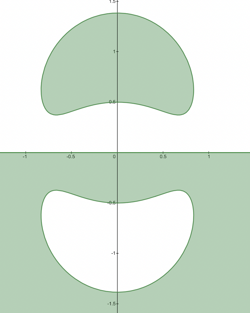
Figure 3: The classification of $\text{sign Im}\theta$. In the green regions, $\text{Im}\theta>0$, which implies that $|e^{2it\theta}|\to 0$ as $t\to\infty$.While in the white regions, $\text{Im}\theta<0$, which implies $|e^{-2it\theta}|\to 0$ as $t\to\infty$. The green curves $\text{Im}\theta=0$ are critical lines between decay and growth regions.

Notice that the division above omits two critical cases : $\xi=-\frac{1}{4}$ and $\xi=2$. For the sake of completeness of the discussion, we will place these two cases in Section 5.

For the cases I and IV, there is no stationary phase point on the real axis, while for the cases II and III, there exist four and two stationary phase points on the real axis, denoted as $\xi_{1}>\xi_{2}>\xi_{3}>\xi_{4}$ and $\xi_{1}>\xi_{2}$ respectively.

The jump matrix $V(k)$ admits the following two factorizations

$$V(k) =\left(\begin{array}[]{cc}1&0\\ -\bar{r}e^{2it\theta}&1\end{array}\right)\left(\begin{array}[]{cc}1&re^{-2it\theta}\\ 0&1\end{array}\right)$$ (2.149)

$$=\left(\begin{array}[]{cc}1&\frac{re^{-2it\theta}}{1-|r|^{2}}\\ 0&1\end{array}\right)(1-|r|^{2})^{-\sigma_{3}}\left(\begin{array}[]{cc}1&0\\ \frac{-\bar{r}e^{2it\theta}}{1-|r|^{2}}&1\end{array}\right).$$ (2.154)

We will utilize these factorizations to open the jump contours so that the oscillating factor $e^{\pm 2it\theta}$ are decaying in corresponding region respectively.

3 Long-time asymptotics in region without phase point

3.1 Deformation of the RH problem

One will observe that the long time asymptotic of RHP 1 is influenced by the growth and decay of the oscillatory term. In this subsection, our aim is to introduce a transform of $M(k;x,t)\rightarrow M^{(1)}(k;x,t)$ so that $M^{(1)}(k;x,t)$ is well behaved as $t\rightarrow\infty$ along the characteristic line.

3.1.1 Conjugation

For $\xi<-\frac{1}{4}$ and $\xi>2$, we choose the decomposition (2.149) , (2.154) respectively. Introduce the notation that will be used later. Define

$$\Delta^{+}=\{ik_{n}|Im\theta(ik_{n})\geq 0,k_{n}\in\mathbb{R}^{+}\}$$

$$\Delta^{-}=\{ik_{n}|Im\theta(ik_{n})<0,k_{n}\in\mathbb{R}^{+}\}$$ (3.1)

and

$$\Lambda=\{ik_{n}||ik_{n}-i\kappa_{1}|<\rho\},\hskip 8.5359pt\{\kappa_{1},-\kappa_{1}\}=i\mathbb{R}\cap\{k|Im\theta(k)=0\},$$

$$\rho=\frac{1}{2}min\{min|ik_{j}-ik_{l}|,min|ik_{j}-\frac{i}{2}|,min|ik_{j}-i\kappa_{1}|\}.$$

Denote

$$L(\xi)=\left\{\begin{array}[]{ll}\emptyset,&\text{as }\xi<-1/4,\\[4.0pt] \mathbb{R},&\text{as }\xi>2,\\ \end{array}\right.$$ (3.4)

where $\emptyset$ means that for any function $f(x)$, we make a definition of engagement

$$\int_{\emptyset}f(x)dx=0.$$

Define the function

$$T(k)=\prod_{ik_{n}\in\Delta^{+}}\frac{k+ik_{n}}{k-ik_{n}}\delta(k,\xi),$$ (3.5)

where

$$\delta(k,\xi)=exp\{-i\int_{L(\xi)}\frac{\mu(s)}{s-k}ds\},\ \ \ \ \mu(k)=\frac{1}{2\pi}log(1-|r|^{2}).$$

Proposition 9.

The function $T(k)$ defined by (3.5) has the following properties:
(a) $T(k)$ is meromorphic in $\mathbb{C}$, and for each $ik_{n}\in\Delta^{+}$, $T(k)$ has simple poles at $ik_{n}$ and simple zeros at $-ik_{n}$; $T(k)$ is analytic and nonzero elsewhere.
(b) $\overline{T(\bar{k})}=\frac{1}{T(k)}$;
(c) $\lim_{k\to\infty}T(k)=1$;
(d) $T(k)$ has boundary values $T_{\pm}(k)$ satisfying:

$$T_{+}(k)=(1-|r(k)|^{2})T_{-}(k),\hskip 14.22636pt\xi>2,$$ (3.6)

$$T_{+}(k)=T_{-}(k),\hskip 14.22636pt\xi<-\frac{1}{4};$$ (3.7)

(e) For $k=\frac{i}{2}$

$$T(\frac{i}{2})=\prod_{ik_{n}\in\Delta^{+}}\frac{\frac{i}{2}+ik_{n}}{\frac{i}{2}-ik_{n}}\delta(\frac{i}{2},\xi);$$

(f) As $k\to\frac{i}{2}$, $T(k)$ has asymptotic expansion as

$$T(k) :=T(\frac{i}{2})+T_{1}(k-\frac{i}{2})+\mathcal{O}((k-\frac{i}{2})^{2}),$$ (3.8)

with

$$T_{1}=\sum_{j,s=1;j\neq s}^{\mathcal{N}(\Delta^{+})}\left(\frac{-2ik_{n_{s}}(ik_{n_{j}}+\frac{i}{2})}{(\frac{i}{2}-ik_{n_{j}})(\frac{i}{2}-ik_{n_{s}})^{2}}\right)J_{0}+\prod_{ik_{n}\in\Delta^{+}}\frac{\frac{i}{2}+ik_{n}}{\frac{i}{2}-ik_{n}}J_{1},$$ (3.9)

where

$$J_{0}=\exp\{-\frac{i}{2\pi}\int_{L(\xi)}\frac{ln(1-|r(s)|^{2})}{s-\frac{i}{2}}ds\};$$ (3.10)

$$J_{1}=-\frac{i}{2\pi}\int_{L(\xi)}\frac{ln(1-|r(s)|^{2})}{(s-\frac{i}{2})^{2}}ds\}.$$ (3.11)

Proof.

Properties (a)-(e) are obtained by simple calculation from the definition of $T(k)$ in (3.5). Property (f) is from the Laurent expansion of $T(k)$ at $k=\frac{i}{2}$. ∎

We define a new unknown function $M^{(1)}(k)$ using the function defined above

$$M^{(1)}(k)=M^{J}(k)T^{\sigma_{3}}(k),$$

then $M^{(1)}$ solves the following RH problem:

RHP 3.

Find a matrix-valued function $M^{(1)}(k)$ which satisfies:

$\blacktriangleright$ Analyticity: $M^{(1)}(k)$ is analytic in $\mathbb{C}\setminus(\mathbb{R}\bigcup\mathcal{Z})$ and has single poles;

$\blacktriangleright$ Jump condition: $M^{(1)}(k)$ has continuous boundary values $M^{(1)}_{\pm}(k)$ on $\mathbb{R}$ and

$$M_{+}^{(1)}(k)=M_{-}^{(1)}(k)V^{(1)}(k,\xi),\hskip 14.22636ptk\in\mathbb{R},$$ (3.12)

where

$$V^{(1)}(k,\xi)=\left\{\begin{array}[]{ll}\left(\begin{array}[]{cc}1&0\\ -T^{2}\overline{r}e^{2it\theta}&1\end{array}\right)\left(\begin{array}[]{cc}1&T^{-2}re^{-2it\theta}\\ 0&1\end{array}\right),&\text{as }\xi<-\frac{1}{4},k\in\mathbb{R},\\[12.0pt] \left(\begin{array}[]{cc}1&\frac{r(k)e^{-2it\theta}T_{-}^{-2}(k)}{1-|r(k)|^{2}}\\ 0&1\end{array}\right)\left(\begin{array}[]{cc}1&0\\ \frac{-\bar{r}(k)e^{2it\theta}T_{+}^{2}(k)}{1-|r(k)|^{2}}&1\end{array}\right),&\text{as }\xi>2,k\in\mathbb{R};\\[12.0pt] \end{array}\right.$$ (3.13)

$\blacktriangleright$ Asymptotic behaviors:

$$M^{(1)}(k)=I+\mathcal{O}(k^{-1}),\hskip 14.22636ptk\rightarrow\infty;$$ (3.14)

$\blacktriangleright$ Residue conditions: $M^{(1)}(k)$ has simple poles at each point in $\mathcal{Z}$ with:

$$\operatorname*{Res}_{k=ik_{n}}M^{(1)}(k)=\left\{\begin{array}[]{ll}\lim_{k\rightarrow ik_{n}}M^{(1)}(k)\left(\begin{array}[]{cc}0&0\\ c_{n}^{-1}e^{2it\theta{(ik_{n})}}[(\frac{1}{T})^{{}^{\prime}}(ik_{n})]^{-2}&0\end{array}\right),&\text{as }ik_{n}\in\Delta^{+},\\[12.0pt] \lim_{k\rightarrow ik_{n}}M^{(1)}(k)\left(\begin{array}[]{cc}0&c_{n}T^{-2}e^{-2it\theta{(ik_{n})}}\\ 0&0\end{array}\right),&\text{as }ik_{n}\in\Delta^{-}\bigcup\Lambda;\\[12.0pt] \end{array}\right.$$ (3.21)

$$\operatorname*{Res}_{k=-ik_{n}}M^{(1)}(k)=\left\{\begin{array}[]{ll}\lim_{k\rightarrow-ik_{n}}M^{(1)}(k)\left(\begin{array}[]{cc}0&\bar{c}_{n}^{-1}e^{-2it\theta{(-ik_{n})}}[T^{{}^{\prime}}(-ik_{n})]^{-2}\\ 0&0\end{array}\right),&\text{as }ik_{n}\in\Delta^{+},\\[12.0pt] \lim_{k\rightarrow-ik_{n}}M^{(1)}(k)\left(\begin{array}[]{cc}0&0\\ \bar{c}_{n}T^{2}e^{2it\theta{(-ik_{n})}}&0\end{array}\right),&\text{as }ik_{n}\in\Delta^{-}\bigcup\Lambda.\\[12.0pt] \end{array}\right.$$ (3.28)

3.1.2 A mixed $\bar{\partial}$-RH problem

The next step is to introduce factorizations of the jump matrix whose factors admit continuous-but not necessarily analytic-extensions off the real axis. The price we pay for this non-analytic transformation is that the new unknown matrix has nonzero $\bar{\partial}$-derivatives inside the regions in which the extensions are introduced and satisfies a hybrid $\bar{\partial}$-RH problem.

Define the domain and contour as follows:

$$\Omega_{2n+1}=\left\{k\in\mathbb{C}|n\pi\leq\arg k\leq n\pi+\varphi\right\},$$

$$\Omega_{2n+2}=\left\{k\in\mathbb{C}|(n+1)\pi-\varphi\leq\arg k\leq(n+1)\pi\right\},$$

where $n=0,1$. And

$$\Sigma_{k}=e^{(k-1)i\pi/2+i\varphi}R_{+},\hskip 14.22636ptk=1,3,$$

$$\Sigma_{k}=e^{ki\pi/2-i\varphi}R_{+},\hskip 14.22636ptk=2,4,$$

which is the boundary of $\Omega_{k}$ respectively. Take $\varphi$ be a sufficiently small fixed angle achieving following conditions:
(i) each $\Omega_{i}$ doesn’t intersect $\left\{k\in\mathbb{C}|\text{Im }\theta(k)=0\right\}$,
(ii) $\cos 2\varphi>\frac{(-1+\sqrt{1-\frac{2}{\xi}})^{2}-2}{2}$ for $\xi<-\frac{1}{4}$;
(iii) $\frac{(1-\sqrt{1-\frac{2}{\xi}})^{2}-2}{2}<\cos 2\varphi<\frac{(1+\sqrt{1-\frac{2}{\xi}})^{2}-2}{2}$ for $\xi>2$.

A more intuitive expression of the above process can be seen in the figure 4.

Figure 4: Figures (a) and (b) corresponding to the cases $\xi<-1/4$ and $\xi>2$ respectively. The blue regions have same decay/grow properties; The same for yellow regions.

Define a new unknown function

$$R^{(2)}(k,\xi)=\left\{\begin{array}[]{lll}\left(\begin{array}[]{cc}1&R_{j}(k,\xi)e^{-2it\theta}\\ 0&1\end{array}\right),&\xi<-\frac{1}{4},k\in\Omega_{j},j=1,2;\\ \\ \left(\begin{array}[]{cc}1&0\\ R_{j}(k,\xi)e^{2it\theta}&1\end{array}\right),&\xi<-\frac{1}{4},k\in\Omega_{j},j=3,4;\\ \\ \left(\begin{array}[]{cc}1&0\\ R_{j}(k,\xi)e^{2it\theta}&1\end{array}\right),&\xi>2,k\in\Omega_{j},j=1,2;\\ \\ \left(\begin{array}[]{cc}1&R_{j}(k,\xi)e^{-2it\theta}\\ 0&1\end{array}\right),&\xi>2,k\in\Omega_{j},j=3,4;\\ \\ I,&elsewhere,\\ \end{array}\right.$$ (3.29)

where the $R_{j}$ are given in the following Proposition.

Proposition 10.

The functions $R_{j}$: $\bar{\Omega}_{j}\to C$, $j=1,2,3,4$ have boundary values as follows:
For $\xi\in(-\infty,-1/4)$,

$$R_{j}(k,\xi)=\Bigg{\{}\begin{array}[]{ll}-r(k)T^{-2}(k)&k\in\mathbb{R}^{i},\\ -r(0)T^{-2}(0)&k\in\Sigma_{j},\\ \end{array}\hskip 17.07182ptj=1,2$$ (3.32)

$$R_{j}(k,\xi)=\Bigg{\{}\begin{array}[]{ll}-\bar{r}(k)T^{2}(k)&k\in\mathbb{R}^{i},\\ -\bar{r}(0)T^{2}(0)&k\in\Sigma_{j},\\ \end{array}\hskip 17.07182ptj=3,4.$$ (3.35)

For $\xi\in(2,+\infty)$,

$$R_{j}(k,\xi)=\Bigg{\{}\begin{array}[]{ll}\frac{\bar{r}}{1-|r(k)|^{2}}T_{+}^{2}&k\in\mathbb{R}^{i},\\ \bar{r}(0)exp\{\frac{1}{\pi i}\int_{\mathbb{R}}\frac{\log{(1-|r|^{2})}}{s}ds\}&k\in\Sigma_{j},\\ \end{array}\hskip 17.07182ptj=1,2$$ (3.38)

$$R_{j}(k,\xi)=\Bigg{\{}\begin{array}[]{ll}\frac{r}{1-|r(k)|^{2}}T_{-}^{-2}&k\in\mathbb{R}^{i},\\ -r(0)exp\{\frac{1}{\pi i}\int_{\mathbb{R}}\frac{\log{(1-|r|^{2})}}{s}ds\}&k\in\Sigma_{j},\\ \end{array}\hskip 17.07182ptj=3,4.$$ (3.41)

where

$$i=\Bigg{\{}\begin{array}[]{ll}+,&j=1,4,\\ -,&j=2,3.\\ \end{array}$$ (3.44)

$R_{j}$ have the following properties: for $j=1,2,3,4,$

$$|\bar{\partial}R_{j}(k)|\lesssim|r^{\prime}(|k|)|+|k|^{-1/2},\ \text{for all $k\in\Omega_{j}$, j=1,2,}$$ (3.45)

$$|\bar{\partial}R_{j}(k)|\lesssim|\bar{r}{{}^{\prime}}(|k|)|+|k|^{-1/2},\ \text{for all $k\in\Omega_{j}$, j=3,4}$$ (3.46)

$$\bar{\partial}R_{j}(k)=0,\hskip 14.22636pt\text{if }k\in elsewhere.$$ (3.47)

Proof.

The proof is similar with [58]. Here, we only take $R_{1}(k)$ of Case IV as an example. By Plemelj formula, the boundary value on $\mathbb{R}^{+}$ of $R_{1}(k)$ can be rewritten as

$$\tilde{r}(k):=\frac{\bar{r}(k)}{1-|r(k)|^{2}}T_{+}^{2}=\prod_{ik_{n}\in\Delta^{+}}\left(\frac{k+ik_{n}}{k-ik_{n}}\right)^{2}\bar{r}(k)exp\{\frac{1}{\pi i}\int_{\mathbb{R}}\frac{\log{(1-|r|^{2})}}{s}ds\}.$$

Construct a continuous function $R_{1}(k)$ on $\Omega_{1}$:

$$R_{1}(k)=\left(\tilde{r}(|k|)-\tilde{r}(0)\right)cos(\frac{\pi}{2\varphi}\phi)+\tilde{r}(0).$$ (3.48)

Denote $k=\rho e^{i\phi}$, then $\bar{\partial}=\frac{e^{i\phi}}{2}\left(\partial_{\rho}+i\rho^{-1}\partial_{\phi}\right)$. So

$$\bar{\partial}R_{1}(k) =\frac{1}{2}\overline{r^{{}^{\prime}}(|k|)}e^{i\phi}\prod_{ik_{n}\in\Delta^{+}}\left(\frac{k+ik_{n}}{k-ik_{n}}\right)^{2}exp\{\frac{1}{\pi i}\int_{\mathbb{R}}\frac{\log{(1-|r|^{2})}}{s}ds\}cos(\frac{\pi}{2\varphi}\phi)$$

$$\quad-\frac{1}{2}e^{i\phi}\rho^{-1}\left(\tilde{r}(|k|)-\tilde{r}(0)\right)sin\left(\frac{\pi}{2\varphi}\phi\right)\frac{\pi}{2\varphi}.$$ (3.49)

By Holder inequality, we bound the second term and then get the estimates. ∎

Make the matrix transformation:

$$M^{(2)}(k)=M^{(1)}(k)R^{(2)}(k),$$

then $M^{(2)}$ solves the mixed $\bar{\partial}$-RH problem:

RHP 4.

Find a matrix valued function $M^{(2)}(k)$ with following properties:

$\blacktriangleright$ Analyticity: $M^{(2)}(k)$ is continuous in $\mathbb{C}\backslash(\Sigma^{(2)}\cup\mathcal{Z})$, where $\Sigma^{(2)}=\cup_{j=1}^{4}\Sigma_{j}$;

$\blacktriangleright$ Jump condition: $M^{(2)}(k)$ has continuous boundary values $M^{(2)}_{\pm}(k)$ on $\Sigma^{(2)}$ and

$$M^{(2)}_{+}(k)=M^{(2)}_{-}(k)V^{(2)}(k),\hskip 14.22636ptk\in\Sigma^{(2)},$$ (3.50)

where

$$V^{(2)}(k,\xi)=\Bigg{\{}\begin{array}[]{ll}R^{(2)}(k)^{-1}|_{\Sigma_{1}\cup\Sigma_{3}}&\text{as }k\in\Sigma_{1}\cup\Sigma_{3};\\[12.0pt] R^{(2)}(k)|_{\Sigma_{2}\cup\Sigma_{4}}&\text{as }k\in\Sigma_{2}\cup\Sigma_{4};\\[12.0pt] \end{array}$$ (3.53)

$\blacktriangleright$ Asymptotic behaviors:

$$M^{(2)}(k)=I+\mathcal{O}(k^{-1}),\hskip 14.22636ptk\rightarrow\infty;$$ (3.54)

$\blacktriangleright$ $\bar{\partial}$-Derivative: For $k\in\mathbb{C}$ we have

$$\bar{\partial}M^{(2)}(k)=M^{(2)}(k)\bar{\partial}R^{(2)}(k),$$ (3.55)

where

$$\bar{\partial}R^{(2)}(k,\xi)=\left\{\begin{array}[]{lll}\left(\begin{array}[]{cc}0&\bar{\partial}R_{j}(k,\xi)e^{-2it\theta}\\ 0&0\end{array}\right),&\xi<-\frac{1}{4},k\in\Omega_{j},j=1,2;\\ \\ \left(\begin{array}[]{cc}0&0\\ \bar{\partial}R_{j}(k,\xi)e^{2it\theta}&0\end{array}\right),&\xi<-\frac{1}{4},k\in\Omega_{j},j=3,4;\\ \\ \left(\begin{array}[]{cc}0&0\\ \bar{\partial}R_{j}(k,\xi)e^{2it\theta}&0\end{array}\right),&\xi>2,k\in\Omega_{j},j=1,2;\\ \\ \left(\begin{array}[]{cc}0&\bar{\partial}R_{j}(k,\xi)e^{-2it\theta}\\ 0&0\end{array}\right),&\xi>2,k\in\Omega_{j},j=3,4;\\ \\ 0,&elsewhere;\\ \end{array}\right.$$ (3.56)

$\blacktriangleright$ Residue conditions: $M^{(2)}$(k) has the same residue conditions with the RHP 3.

In order to solve the RHP 4, we decompose it into a pure RH problem $M^{(R)}(k)$ with $\bar{\partial}R^{(2)}\equiv 0$ and a pure $\bar{\partial}$ problem $M^{(3)}(k)$ with $\bar{\partial}R^{(2)}\not=0$, that is,

$$M^{(2)}(k)=M^{(3)}(k)M^{(R)}(k),$$ (3.57)

where the matrix function $M^{(R)}$ satisfies

RHP 5.

Find a matrix valued function $M^{(R)}(k)$ admits same condition as RHP 4.

$\blacktriangleright$ Analyticity: $M^{(R)}(k)$ is meromorphic in $\mathbb{C}\backslash\Sigma^{(2)}$;

$\blacktriangleright$ Jump condition: $M^{(R)}(k)$ has the same jump matrix with $M^{(2)}(k)$ ;

$\blacktriangleright$ Asymptotic behaviors:

$$M^{(R)}(k)=I+\mathcal{O}(k^{-1}),\hskip 14.22636ptk\rightarrow\infty;$$ (3.58)

$\blacktriangleright$ Residue conditions: $M^{(R)}$(k) has the same residue conditions with the RHP 3.

3.2 Analysis on a pure RH problem

3.2.1 Classify the poles

In this section, our aim is to convert the poles away from $\left\{k\in\mathbb{C}|\text{Im }\theta(k)=0\right\}$ into jumps.

Define

$$G(k)=\left\{\begin{array}[]{ll}\left(\begin{array}[]{cc}1&0\\ -c_{n}^{-1}T(k)e^{2it\theta(ik_{n})}[(\frac{1}{T})^{{}^{\prime}}(ik_{n})]^{-1}&1\end{array}\right),&\text{as }k\in\partial\mathcal{D}_{n},ik_{n}\in\Delta^{+};\\[12.0pt] \left(\begin{array}[]{cc}1&c_{n}T^{-2}e^{-2it\theta(ik_{n})}(k-ik_{n})^{-1}\\ 0&1\end{array}\right),&\text{as }k\in\partial\mathcal{D}_{n},ik_{n}\in\Delta^{-};\\[12.0pt] \left(\begin{array}[]{cc}1&-\bar{c}_{n}^{-1}T^{-1}e^{-2it\theta(-ik_{n})}[T^{{}^{\prime}}(-ik_{n})]^{-1}\\ 0&1\end{array}\right),&\text{as }k\in\partial\bar{\mathcal{D}}_{n},ik_{n}\in\Delta^{+};\\[12.0pt] \left(\begin{array}[]{cc}1&0\\ \bar{c}_{n}T^{2}e^{2it\theta(-ik_{n})}(k+ik_{n})^{-1}&1\end{array}\right),&\text{as }k\in\partial\bar{\mathcal{D}}_{n},ik_{n}\in\Delta^{-};\\[12.0pt] I,&\text{elsewhere }.\end{array}\right.$$ (3.59)

and make a transformation

$$M_{R}(k)=M^{(R)}(k)G(k),$$ (3.60)

then $M_{R}(k)$ satisfies the following RH problem:

RHP 6.

Find a matrix valued function $M_{R}(k)$ with following properties:

$\blacktriangleright$ Analyticity: $M_{R}(k)$ is meromorphic in $\mathbb{C}\backslash\Sigma_{R}$;

$\blacktriangleright$ Jump condition:

$$M_{+,R}(k)=M_{-,R}(k)V_{R}(k),\hskip 14.22636ptk\in\Sigma_{R};$$

where

$$V_{R}(k)=\Bigg{\{}\begin{array}[]{ll}V^{(2)}(k),&\text{as }k\in\Sigma^{(2)};\\[12.0pt] G(k),&\text{as }k\in\bigcup_{\{n|ik_{n}\in(\mathbb{C}^{+}\cap\mathcal{Z})\backslash\Lambda\}}\left(\partial\mathcal{D}_{n}\cup\partial\bar{\mathcal{D}}_{n}\right);\end{array}$$

The $\Sigma_{R}$ is shown in Figure 5.

$\blacktriangleright$ Asymptotic behaviors:

$$M_{R}(k)= I+\mathcal{O}(k^{-1}),\hskip 14.22636ptk\rightarrow\infty;$$

$\blacktriangleright$ Residue conditions:

$$\operatorname*{Res}_{k=ik_{n}}M_{R}(k)=\lim_{k\rightarrow ik_{n}}M_{R}(k)\left(\begin{array}[]{cc}0&c_{n}T^{-2}e^{-2it\theta{(ik_{n})}}\\ 0&0\end{array}\right), \text{as }\hskip 5.69046ptik_{n}\in\Lambda;$$ (3.64)

$$\operatorname*{Res}_{k=-ik_{n}}M_{R}(k)=\lim_{k\rightarrow-ik_{n}}M_{R}(k)\left(\begin{array}[]{cc}0&0\\ \bar{c}_{n}T^{2}e^{2it\theta{(-ik_{n})}}&0\end{array}\right), \text{as }\hskip 5.69046ptik_{n}\in\Lambda;$$ (3.67)

Figure 5: (a), (b) show the Jump path of $M_{R}$ under the condition $\xi<-1/4$ and $\xi>2$ respectively. $\Sigma_{R}$ composed of the blue circles and lines in the figure.

Next, we prove the existence and uniqueness of solution of the above RHP 6.

Proposition 11.

For any given scattering data $\mathcal{D}=\{r(k),\{ik_{n},c_{n}\}_{n\in\aleph}\}$, the solution $M_{R}(k)$ of the above RH problem exists uniquely and is equivalent to the RHP 1 corresponding to the reflection-free N soliton solution of the corrected scattering data $\tilde{\mathcal{D}}=\{\tilde{r}=0,\{ik_{n},\tilde{c}_{n}\}_{n\in\aleph}\}$ by a display transformation, where the correlation function $\tilde{c}_{n}=c_{n}\delta(ik_{n})$.

Proof.

$M_{R}(k)$ contains a number of jump lines consisting of small circles and poles in $\Lambda$. Take a transformation

$$\hat{M}(k)=M_{R}(k)G^{-1}(k)\left(\prod_{ik_{n}\in\Delta^{+}}\frac{k+ik_{n}}{k-ik_{n}}\right)^{-\sigma_{3}},$$ (3.68)

then
a. $\hat{M}(k)$ is asymptotic to I when $k\rightarrow\infty$;
b. $\hat{M}(k)$ has no jump on the small circles ;
c. When $ik_{n}\not\in\Lambda$, the transformation converts the jump into the poles. For $ik_{n}\in\Lambda$,

$$\operatorname*{Res}_{k=ik_{n}}\hat{M}(k)=\operatorname*{Res}_{k=ik_{n}}M_{R}(k)G^{-1}(k)\left(\prod_{ik_{n}\in\Delta^{+}}\frac{k+ik_{n}}{k-ik_{n}}\right)^{-\sigma_{3}}$$

$$= \lim_{k\rightarrow ik_{n}}\hat{M}(k)\left(\prod_{ik_{n}\in\Delta^{+}}\frac{k+ik_{n}}{k-ik_{n}}\right)^{-\sigma_{3}}\left(\begin{array}[]{cc}0&c_{n}T^{-2}e^{-2it\theta{(ik_{n})}}\\ 0&0\end{array}\right)G^{-1}(k)\left(\prod_{ik_{n}\in\Delta^{+}}\frac{k+i}{k-ik_{n}}\right)^{-\sigma_{3}}$$ (3.71)

$$= \lim_{k\rightarrow ik_{n}}\hat{M}(k)\left(\begin{array}[]{cc}0&c_{n}\delta(ik_{n})e^{-2it\theta{(ik_{n})}}\\ 0&0\end{array}\right),$$ (3.74)

thus, $\tilde{c}_{n}=c_{n}\delta(ik_{n})$;

So far, we have proved that $\hat{M}(k)$ is the solution of RHP 1 under the corrected scattering data $\tilde{\mathcal{D}}=\{\tilde{r}=0,\{ik_{n},c_{n}\delta(ik_{n})\}_{ik_{n}\in\aleph}\}$. And the solution of this kind of RH problem is existentially unique, so $M_{R}(k)$ exists uniquely. ∎

3.2.2 Soliton solutions

Let $M^{\Lambda}(k)$ denote the RH problem for $M_{R}(k)$ without jumps, then $M^{\Lambda}(k)$ satisfies

RHP 7.

Find a matrix valued function $M^{\Lambda}(k)$ with following properties:

$\blacktriangleright$ Analyticity: $M^{\Lambda}(k)$ is meromorphic in $\mathbb{C}$;

$\blacktriangleright$ $\bar{\partial}$-Derivative: $\bar{\partial}R^{(2)}(k)=0$;

$\blacktriangleright$ Asymptotic behaviors:

$$M^{\Lambda}(k)= I+\mathcal{O}(k^{-1}),\hskip 14.22636ptk\rightarrow\infty;$$

$\blacktriangleright$ Residue conditions: $M^{\Lambda}$(k) has the same residue conditions with the RHP 6.

Proposition 12.

For any given corrected scattering data $\tilde{\mathcal{D}}_{\Lambda}=\{\tilde{r}=0,\{ik_{n},\tilde{c}_{n}\},ik_{n}\in\Lambda\}$, the solution of RHP 7 exists uniquely and is shown to be constructed:
I: if $\Lambda=\varnothing$, then

$$M^{\Lambda}(k)=I;$$ (3.75)

II: if $\Lambda\neq\varnothing$ with $\Lambda=\left\{ik_{n}\right\}_{n=1}^{\Xi}$, where the symbol $\Xi$ denotes the number of poles in $\Lambda$, then

$$M^{\Lambda}(k) =I+\sum_{n=1}^{\Xi}\left(\begin{array}[]{cc}\frac{\gamma_{n}}{k+ik_{n}}&\frac{\beta_{n}}{k-ik_{n}}\\ \frac{\zeta_{n}}{k+ik_{n}}&\frac{\alpha_{n}}{k-ik_{n}}\end{array}\right).$$ (3.78)

Here $\alpha_{n},\beta_{n},\gamma_{n},\zeta_{n}$ are determined by linearly dependant equations:

$$c_{n}^{-1}T^{2}(ik_{n})e^{2it\theta{(ik_{n})}}\beta_{n}=1+\sum_{h=1}^{\Xi}\frac{\gamma_{h}}{ik_{n}+ik_{h}},$$ (3.79)

$$c_{n}^{-1}T^{2}(ik_{n})e^{2it\theta{(ik_{n})}}\alpha_{n}=\sum_{h=1}^{\Xi}\frac{\zeta_{h}}{ik_{n}+ik_{h}},$$ (3.80)

$$c_{n}^{-1}T^{2}(ik_{n})e^{2it\theta{(ik_{n})}}\gamma_{n}=\sum_{h=1}^{\Xi}\frac{-\beta_{h}}{ik_{n}+ik_{h}},$$ (3.81)

$$c_{n}^{-1}T^{2}(ik_{n})e^{2it\theta{(ik_{n})}}\zeta_{n}=1+\sum_{h=1}^{\Xi}\frac{-\alpha_{h}}{ik_{n}+ik_{h}}.$$ (3.82)

Proof.

The uniqueness of solution follows from the Liouville’s theorem. The result of I can be simple obtain.

As for II, the residue and asymptotic conditions ensure that $M^{\Lambda}(k)$ can have an expansion of the form as mentioned above. $\alpha_{n},\beta_{n},\gamma_{n},\zeta_{n}$ are obtained from four linearly dependant equations (3.79)-(3.82) which come from substituting (3.78) into (3.64). ∎

For convenience, denote the asymptotic expansion of $M^{\Lambda}(k)$ as $k\to\frac{i}{2}$:

$$M^{\Lambda}(k)=M^{\Lambda}(\frac{i}{2})+M^{\Lambda}_{1}(k-\frac{i}{2})+\mathcal{O}((k-\frac{i}{2})^{2}).$$ (3.83)

3.2.3 Error estimate between $M_{R}$ and $M^{\Lambda}$

Here we try to match $M_{R}(k)$ to the soliton solution $M^{\Lambda}(k)$ and show that the error between the two is a small norm RHP. We define $M^{err}$ as the error between $M_{R}$ and $M^{\Lambda}$ with

$$M^{err}(k)=M_{R}(k)\left(M^{\Lambda}(k)\right)^{-1},$$ (3.84)

which satisfies the following RH problem

RHP 8.

Find a matrix-valued function $M^{err}(k)$ with following identities:

$\blacktriangleright$ Analyticity: $M^{err}(k)$ is analytical in $\mathbb{C}\setminus\Sigma_{R}$;

$\blacktriangleright$ Asymptotic behaviors:

$$M^{err}(k)\sim I+\mathcal{O}(k^{-1}),\hskip 14.22636pt|k|\rightarrow\infty;$$ (3.85)

$\blacktriangleright$ Jump condition: $M^{err}(k)$ has continuous boundary values $M^{err}_{\pm}(k)$ on $\Sigma_{R}$ satisfying

$$M^{err}_{+}(k)=M^{err}_{-}(k)V^{err}(k),$$

where the jump matrix $V^{err}(k)$ is given by

$$V^{err}(k)=M^{\Lambda}(k)V_{R}(k)M^{\Lambda}(k)^{-1}.$$ (3.86)

Lemma 4.

The jump matrix $V_{R}(k)$ defined by (3.59) satisfies

$$\parallel V_{R}(k)-I\parallel_{L^{\infty}(\Sigma_{R}\setminus\Sigma^{(2)})}=\mathcal{\mathcal{O}}(e^{-2\rho_{0}t}),$$ (3.87)

where

$$\rho_{0}=\min_{ik_{n}\in\Delta\setminus\Lambda}\left\{|\text{Im}\theta_{n}|>\delta_{0}\right\}.$$ (3.88)

Proof.

Take $k\in\{k:|k-ik_{n}|=\rho,ik_{n}\in\Delta^{+}\}$ as an example.

$$\parallel V_{R}(k)-I\parallel_{L^{\infty}} =|c_{n}^{-1}T(k)e^{2it\theta(ik_{n})}[(\frac{1}{T})^{{}^{\prime}}(ik_{n})]^{-1}|$$

$$\lesssim e^{-\text{Re}(2it\theta_{n})}\lesssim e^{2t\text{Im}(\theta_{n})}\leq e^{-2\rho_{0}t}.$$

The proofs for the rest of the cases are similar. ∎

Corollary 1.

For $1\leq p\leq+\infty$, the jump matrix $V_{R}(k)$ satisfies

$$\parallel V_{R}(k)-I\parallel_{L^{p}(\Sigma_{R}\setminus\Sigma^{(2)})}\leq C_{p}e^{-2\rho_{0}t},$$ (3.89)

$$\parallel V_{R}(k)-I\parallel_{L^{p}(\Sigma^{(2)})}\leq C_{p}t^{-\frac{1}{p}},$$ (3.90)

where $C_{p}\geq 0$ depends on $p$.

Lemma 5.

The jump matrix $V^{err}(k)$ satisfies

$$\parallel V^{err}(k)-I\parallel_{L^{\infty}(\Sigma_{R}\setminus\Sigma^{(2)})}=\mathcal{\mathcal{O}}(e^{-2\rho_{0}t}),$$ (3.91)

Proof.

Take $k\in\{k:|k-ik_{n}|=\rho,ik_{n}\in\Delta^{+}\}$ as an example.

$$|V_{R}(k)-I|=|M^{\Lambda}(k)(V_{R}-I)M^{\Lambda}(k)^{-1}|\leq c|V_{R}-I|\leq e^{-2\rho_{0}t}.$$

The proofs for the rest of the cases are similar. ∎

Corollary 2.

For $1\leq p\leq+\infty$, the jump matrix $V^{err}(k)$ satisfies

$$\parallel V^{err}(k)-I\parallel_{L^{p}(\Sigma_{R}\setminus\Sigma^{(2)})}\leq C_{p}e^{-2\rho_{0}t},$$ (3.92)

$$\parallel V^{err}(k)-I\parallel_{L^{p}(\Sigma^{(2)})}\leq C_{p}t^{-\frac{1}{p}}.$$ (3.93)

Denote

$$C_{\omega_{e}}f=C_{-}(f(V^{err}-I)),$$ (3.94)

where $C_{-}$ is the Cauchy projection operator, defined as follows

$$C_{-}f(k)=\operatorname*{lim}\limits_{k^{\prime}\to k\in\Sigma_{R}}\frac{1}{2\pi i}\int_{\Sigma^{(2)}}\frac{f(s)}{s-k^{\prime}}ds,$$ (3.95)

and $\|C^{-}\|_{L^{2}}$ is bounded. By Beals-Coifman’s theorem, the solution of the above RH problem can be expressed as

$$M^{err}(k)=I+\frac{1}{2\pi i}\int_{\Sigma_{R}}\frac{\mu_{e}(s)(V^{err}(s)-I)}{s-k}ds,$$ (3.96)

where $\mu_{e}(k)\in L^{2}(\Sigma_{R})$ satisfies

$$(1-C_{\omega_{e}})\mu_{e}(k)=I.$$ (3.97)

Using (3.91)-(3.94), we can see that

$$||C_{\omega_{e}}||_{L^{2}(\Sigma_{R})}\leq||C_{-}||_{L^{2}(\Sigma_{R})}||V^{err}(k)-I||_{L^{\infty}(\Sigma_{R})}\leq ct^{-\frac{1}{2}},$$ (3.98)

which implies that the operator $(1-C_{\omega_{e}})^{-1}$ exists for large $t$, so $\mu_{e}$ and $M^{err}(k)$ exist uniquely. Next we make some estimates and asymptotic behaviors of $M^{err}(k)$.

Proposition 13.

For $M^{err}(k)$ defined in (3.84), it stratifies

$$|M^{err}(k)-I|\leq ct^{-\frac{1}{2}}.$$ (3.99)

When $k=\frac{i}{2}$,

$$M^{err}(\frac{i}{2})=I+\frac{1}{2\pi i}\int_{\Sigma_{R}}\dfrac{\mu_{e}(s)(V^{err}(s)-I)}{s-\frac{i}{2}}ds,$$ (3.100)

As $k\to\frac{i}{2}$, the Laurent expansion of $M^{err}(k)$ is

$$M^{err}(k)=M^{err}(\frac{i}{2})+M_{1}^{err}(k-\frac{i}{2})+\mathcal{O}((k-\frac{i}{2})^{2}),$$ (3.101)

where

$$M_{1}^{err}=\frac{1}{2\pi i}\int_{\Sigma_{R}}\frac{\mu_{e}(s)(V^{err}(s)-I)}{(s-\frac{i}{2})^{2}}ds.$$ (3.102)

In addition, $M^{err}(\frac{i}{2})$ and $M_{1}^{err}$ satisfy following asymptotics

$$|M^{err}(\frac{i}{2})-I|\lesssim\mathcal{O}(t^{-\frac{1}{2}}),\hskip 14.22636ptM_{1}^{err}\lesssim\mathcal{O}(t^{-\frac{1}{2}}).$$ (3.103)

Proof.

By (3.96),

$$M^{err}(k)-I=\frac{1}{2\pi i}\int_{\Sigma_{R}}\frac{V^{err}(s)-I}{s-k}ds+\frac{1}{2\pi i}\int_{\Sigma_{R}}\frac{(\mu_{e}(s)-I)(V^{err}(s)-I)}{s-k}ds,$$

from which the following estimate is obtained

$$|M^{err}(k)-I| \leq\|V^{err}(s)-I\|_{L^{2}(\Sigma_{R})}\|\frac{1}{s-k}\|_{L^{2}(\Sigma_{R})}+$$

$$\ \ \ \ \|V^{err}(s)-I\|_{L^{\infty}(\Sigma_{R})}\|\mu_{e}(s)-I\|_{L^{2}(\Sigma_{R})}\|\frac{1}{s-k}\|_{L^{2}(\Sigma_{R})}$$

$$\leq ct^{-\frac{1}{2}}.$$

(3.101)-(3.102) can be obtained by Taylor expansion. At last, since $(s-\frac{i}{2})^{-2}$ is bounded in $\Sigma_{R}$, the proof of (3.103) is given as follows:

$$|M_{1}^{err}|\lesssim||V^{err}-I||_{L^{2}}||\mu_{e}(s)-I||_{L^{2}}+||V^{err}-I||_{L^{1}}\lesssim\mathcal{O}(t^{-\frac{1}{2}}).$$

∎

3.3 Analysis on a pure $\bar{\partial}$ problem

In this subsection, we mainly consider the following pure $\bar{\partial}$-problem which is defined by (3.57)

RHP 9.

(Pure $\bar{\partial}$-problem) Find $M^{(3)}(k)$ with following identities:

$\blacktriangleright$ Analyticity: $M^{(3)}(k)$ is continuous and has sectionally continuous first partial derivatives in $\mathbb{C}$.

$\blacktriangleright$ Asymptotic behavior:

$$M^{(3)}(k)\sim I+\mathcal{O}(k^{-1}),\hskip 14.22636ptk\rightarrow\infty;$$ (3.104)

$\blacktriangleright$ $\bar{\partial}$-Derivative: We have

$$\bar{\partial}M^{(3)}(k)=M^{(3)}(k)W^{(3)}(k),\ \ k\in\mathbb{C},$$

where

$$W^{(3)}(k)=M^{(R)}(k)\bar{\partial}R^{(2)}(k)M^{(R)}(k)^{-1}.$$ (3.105)

The solution of the pure $\bar{\partial}$ problem $M^{(3)}(k)$ is given by the following integral equation

$$M^{(3)}(k)=I-\frac{1}{\pi}\iint_{\mathbb{C}}\frac{M^{(3)}W^{(3)}}{s-k}\mathrm{d}A(s),$$ (3.106)

where $\mathrm{d}A(s)$ is the Lebesgue measure in the complex plane. The equation (3.106) can also be expressed as an operator equation

$$(I-J)M^{(3)}(k)=I,$$ (3.107)

where $J$ is the Cauchy operator

$$Jf(k)=-\frac{1}{\pi}\iint_{\mathbb{C}}\frac{f(s)W^{(3)}(s)}{s-k}\mathrm{d}A(s).$$ (3.108)

Lemma 6.

For $\xi\in(-\infty,-\frac{1}{4})$, ${\rm Im}\theta(k)$ has following estimation:

$$\text{Im }\theta(k)\leq|k||sin\omega|\left(\xi+\frac{1}{1+cos2\varphi+\sqrt{2(1+cos2\varphi)}}\right),\hskip 14.22636pt\text{as }k\in\Omega_{1},\Omega_{2},$$ (3.109)

$$\text{Im }\theta(k)\geq-|k||sin\omega|\left(\xi+\frac{1}{1+cos2\varphi+\sqrt{2(1+cos2\varphi)}}\right),\hskip 8.5359pt\text{as }k\in\Omega_{3},\Omega_{4}.$$ (3.110)

For $\xi\in(2,+\infty)$, the estimation is shown as follow:

$$\text{Im }\theta(k)\geq|k||sin\omega|\left(\xi+\frac{1}{1+cos2\varphi-\sqrt{2(1+cos2\varphi)}}\right),\hskip 14.22636pt\text{as }k\in\Omega_{1},\Omega_{2},$$ (3.111)

$$\text{Im }\theta(k)\leq-|k||sin\omega|\left(\xi+\frac{1}{1+cos2\varphi-\sqrt{2(1+cos2\varphi)}}\right),\hskip 8.5359pt\text{as }k\in\Omega_{3},\Omega_{4}.$$ (3.112)

Proof.

We just take $k\in\Omega_{1}$ as an example, and the other regions are similarly.

Since $\theta(k)=k\xi-\frac{k}{2k^{2}+\frac{1}{2}}$, let $k=|k|e^{i\omega}=u+iv$, then

$${\rm Im}\theta(k)=ksin\omega\left(\xi+\frac{2|k|^{2}-\frac{1}{2}}{(2|k|^{2}cos2\omega+\frac{1}{2})^{2}+4|k|^{2}sin^{2}2\omega}\right).$$

Denote

$$h(x;a)=\frac{x}{(x+\frac{1}{2})^{2}+a(x+\frac{1}{2})+\frac{1}{4}},$$

where $x=2|k|^{2}-\frac{1}{2}$, $a=cos2\omega$, and then

$$h(x,a)\in\left(-\infty,1+a-\sqrt{2(1+a)}\right)\bigcup\left(1+a+\sqrt{2(1+a)},+\infty\right).$$

From ${\rm Im}\theta=v\left(\xi+h(x;a)\right)$ with $x\in(-\frac{1}{2},+\infty)$, $a\in[cos2\varphi,1]$, the conclusion of the lemma is obtained. ∎

Corollary 3.

There exist constants $c(\xi)<0$, $\tilde{c}(\xi)>0$ relative to $\xi$ that the imaginary part of phase function (2.107) $\text{Im }\theta(k)$ have following evaluation for $k=|k|e^{i\omega}=u+iv$:
When $\xi\in(-\infty,-1/4)$,

$${\rm Im}\theta(k)\leq c(\xi)v,\hskip 14.22636pt\text{as }k\in\Omega_{1},\Omega_{2},$$ (3.113)

$${\rm Im}\theta(k)\geq-c(\xi)v,\hskip 14.22636pt\text{as }k\in\Omega_{3},\Omega_{4}.$$ (3.114)

When $\xi\in(2,+\infty)$,

$${\rm Im}\theta(k)\geq\tilde{c}(\xi)v,\hskip 14.22636pt\text{as }k\in\Omega_{1},\Omega_{2},$$ (3.115)

$${\rm Im}\theta(k)\leq-\tilde{c}(\xi)v,\hskip 14.22636pt\text{as }k\in\Omega_{3},\Omega_{4}.$$ (3.116)

Next we prove that the above operator $J$ is small parametric when $t$ is sufficiently large.

Proposition 14.

To the case $\xi\in(-\infty,-1/4)\cup(2,+\infty)$, for sufficiently large $t$, we have

$$||J||_{L^{\infty}\rightarrow L^{\infty}}\leqslant ct^{-\frac{1}{2}}.$$ (3.117)

Therefore $(1-J)^{-1}$ exists, and thus the operator equation (3.107) has a unique solution.

Proof.

Here, we just take the case $\xi\in(-\infty,-1/4)$ as an example. In order to get the estimate (3.117), it is only need to prove that for $f\in L^{\infty}(\mathbb{C})$,

$$||Jf||_{L^{\infty}(\mathbb{C})}\leqslant ct^{-1/2}||f||_{L^{\infty}(\mathbb{C})}.$$

Here, we just prove the case $k\in\Omega_{1}$. By (3.108),

$$|Jf(k)|\leq c||f||_{L^{\infty}}\iint_{\Omega_{1}}\frac{|W^{(3)}(s)|}{|s-k|}dA(s),$$ (3.118)

where

$$|W^{(3)}(s)| \leq|M^{(R)}||\bar{\partial}R^{(2)}||(M^{(R)})^{-1}|\leq|M^{(R)}||\bar{\partial}R^{(2)}||\sigma_{2}(M^{(R)})^{T}\sigma_{2}|$$

$$\leq|M^{(R)}|^{2}|\bar{\partial}R^{(2)}|\leq c|\bar{\partial}R_{1}(k)||e^{-2it\theta}|,$$ (3.119)

thus

$$\iint_{\Omega_{1}}\frac{|W^{(3)}(s)|}{|s-k|}dA(s)\lesssim\iint_{\Omega_{1}}\frac{|\bar{\partial}R_{1}|e^{2tIm\theta}}{|s-k|}dA(s)$$ (3.120)

Referring into (3.45) in Proposition 10, the integral $\iint_{\Omega_{1}}\frac{|\bar{\partial}R_{1}|e^{2tIm\theta}}{|s-k|}dA(s)$ can be divided to two part:

$$\iint_{\Omega_{1}}\dfrac{|\bar{\partial}R_{1}(s)|e^{2t\text{Im}\theta}}{|s-k|}dA(s)\lesssim I_{1}+I_{2},$$ (3.121)

with

$$I_{1}=\iint_{\Omega_{1}}\dfrac{|r^{\prime}(|s|)|e^{2t\text{Im}\theta}}{|s-k|}dA(s),\hskip 14.22636ptI_{2}=\iint_{\Omega_{1}}\dfrac{|s|^{-1/2}e^{2t\text{Im}\theta}}{|s-k|}dA(s).$$ (3.122)

Denoting $s=u+iv$, $k=k_{R}+ik_{I}$, (3.114) gives that

$$\text{Im }\theta(s)\leq c(\xi)2tv\leq c^{\prime}tv.$$ (3.123)

Therefore,

$$I_{1}=\int_{0}^{\infty}e^{c^{\prime}tv}dv\int_{v}^{\infty}\frac{|r^{\prime}(|s|)|}{|s-k|}du\leq\int_{0}^{\infty}e^{c^{\prime}tv}\|r^{\prime}(|s|)\|_{L^{2}(v,\infty)}\bigg{\|}\frac{1}{s-k}\bigg{\|}_{L^{2}(v,\infty)}dv.$$ (3.124)

Note that

$$\bigg{\|}\frac{1}{s-k}\bigg{\|}^{2}_{L^{2}(v,\infty)}=\int_{v}^{\infty}\frac{1}{|s-k|^{2}}du\leq\int_{-\infty}^{\infty}\frac{1}{(u-k_{R})^{2}+(v-k_{I})^{2}}du$$

$$=\frac{1}{|v-k_{I}|}\int_{-\infty}^{\infty}\frac{1}{1+y^{2}}dy=\frac{\pi}{|v-k_{I}|},$$ (3.125)

where $y=\frac{u-k_{R}}{v-k_{I}}$. And

$$\|r^{\prime}(|s|)\|_{L^{2}(v,\infty)}^{2}=\int_{v}^{\infty}\big{|}r^{\prime}(\sqrt{u^{2}+v^{2}})\big{|}^{2}du\leq\int_{\sqrt{2}v}^{\infty}\big{|}r^{\prime}(\tau)\big{|}^{2}\frac{\sqrt{u^{2}+v^{2}}}{u}d\tau$$

$$\leq\sqrt{2}\int_{\sqrt{2}v}^{\infty}\big{|}r^{\prime}(\tau)\big{|}^{2}d\tau\leq\|r^{\prime}(s)\|_{L^{2}(\mathbb{R})}^{2}.$$ (3.126)

(3.125)-(3.126) implies that

$$I_{1}\leq c\|r^{\prime}\|_{L^{2}(\mathbb{R})}\int_{0}^{\infty}e^{c^{\prime}tv}|v-k_{I}|^{-1/2}dv$$

$$=c\|r^{\prime}\|_{L^{2}(\mathbb{R})}\left[\int_{0}^{k_{I}}\frac{e^{c^{\prime}tv}}{\sqrt{k_{I}-v}}dv+\int_{k_{I}}^{\infty}\frac{e^{c^{\prime}tv}}{\sqrt{v-k_{I}}}dv\right]$$

$$\lesssim t^{-\frac{1}{2}}.$$ (3.127)

To estimate $I_{2}$, we consider the following two $L^{p}$-estimates $(p>2)$.

$$\||s|^{-1/2}\|_{L^{p}(v,\infty)}=\left(\int_{v}^{\infty}\frac{1}{|u+iv|^{p/2}}du\right)^{1/p}=\left(\int_{v}^{\infty}\frac{1}{(u^{2}+v^{2})^{p/4}}du\right)^{1/p}$$

$$=v^{1/p-1/2}\left(\int_{1}^{\infty}\frac{1}{(1+x^{2})^{p/4}}dx\right)^{1/p}\leq cv^{1/p-1/2};$$ (3.128)

$$\big{\|}|s-k|^{-1}\big{\|}_{L^{q}(v,\infty)}\leq c|v-k_{I}|^{1/q-1},\ \ 1/p+1/q=1.\$$ (3.129)

Using the two estimates above, we arrive at

$$I_{2} \leq\int_{0}^{\infty}e^{c^{\prime}tv}dv\int_{v}^{\infty}\frac{|s|^{-1/2}}{|s-k|}du$$

$$\leq\int_{0}^{\infty}e^{c^{\prime}tv}\||s|^{-1/2}\|_{L^{p}(v,\infty)}\big{\|}|s-k|^{-1}\big{\|}_{L^{q}(v,\infty)}dv.$$

$$\leq c\left[\int_{0}^{k_{I}}e^{c^{\prime}tv}v^{1/p-1/2}|v-k_{I}|^{1/q-1}dv+\int_{k_{I}}^{\infty}e^{c^{\prime}tv}v^{1/p-1/2}|v-k_{I}|^{1/q-1}dv\right].$$ (3.130)

Calculating the two integrals yields

$$I_{2}\leq ct^{-\frac{1}{2}}.$$ (3.131)

By (3.118)-(3.121), the result of Proposition 14 is proved. ∎

Proposition 15.

There exist a positive constant $\frac{1}{4}<\rho<\frac{1}{2}$ such that the solution $M^{(3)}(k)$ of $\bar{\partial}$-problem admits the following estimation

$$\parallel M^{(3)}(\frac{i}{2})-I\parallel=\parallel\frac{1}{\pi}\iint_{\mathbb{C}}\dfrac{M^{(3)}(s)W^{(3)}(s)}{s-\frac{i}{2}}dA(s)\parallel\lesssim t^{-\frac{3}{2}+2\rho}.$$ (3.132)

As $k\to\frac{i}{2}$, $M^{(3)}(k)$ has asymptotic expansion

$$M^{(3)}(k)=M^{(3)}(\frac{i}{2})+M^{(3)}_{1}(x,t)(k-\frac{i}{2})+\mathcal{O}((k-\frac{i}{2})^{2}),$$ (3.133)

where $M^{(3)}_{1}(x,t)$ is a $k$-independent coefficient with

$$M^{(3)}_{1}(x,t)=\frac{1}{\pi}\iint_{C}\dfrac{M^{(3)}(s)W^{(3)}(s)}{(s-\frac{i}{2})^{2}}dA(s),$$ (3.134)

and $M^{(3)}_{1}(x,t)$ satisfies

$$|M^{(3)}_{1}(x,t)|\lesssim t^{-\frac{3}{2}+2\rho}.$$ (3.135)

Proof.

First we estimate (3.132). The proof proceeds along the same steps as the proof of above Proposition. (3.107) and (3.117) implies that for large $t$, $\parallel M^{(3)}\parallel_{\infty}\lesssim 1$. And here we only estimate the integral on sector $\Omega_{1}$ as $\xi<-1/4$. Let $s=u+vi$. We also divide $M^{(3)}(\frac{i}{2})-I$ to two parts:

$$\frac{1}{\pi}\iint_{\mathbb{C}}\dfrac{M^{(3)}(s)W^{(3)}(s)}{s-\frac{i}{2}}dA(s)\lesssim I_{3}+I_{4},$$ (3.136)

with

$$I_{3}=\iint_{\Omega_{1}}\dfrac{|r^{\prime}(|s|)|e^{2t\text{Im}\theta}}{|\frac{i}{2}-s|}dA(s),\hskip 14.22636ptI_{4}=\iint_{\Omega_{1}}\dfrac{|s|^{-\frac{1}{2}}e^{2t\text{Im}\theta}}{|\frac{i}{2}-s|}dA(s).$$ (3.137)

For $s\in\Omega_{1}$, there exists a constant $c>0$ so that $|\frac{i}{2}-s|\leq c$. So

$$I_{3}\leq \int_{0}^{+\infty}\int_{v}^{+\infty}\dfrac{|r^{\prime}(|s|)|e^{c^{\prime}tv}}{|\frac{i}{2}-s|}dudv$$

$$\lesssim\int_{0}^{+\infty}\parallel r^{\prime}\parallel_{L^{1}(\mathbb{R}^{+})}e^{c^{\prime}tv}dv\lesssim\int_{0}^{+\infty}e^{c^{\prime}tv}dv\lesssim t^{-1}.$$

As for $I_{4}$, we partition it to two parts:

$$I_{4}\leq\int_{0}^{\frac{1}{4}}\int_{v}^{+\infty}\dfrac{|s|^{-\frac{1}{2}}e^{c^{\prime}tv}}{|\frac{i}{2}-s|}dudv+\int_{\frac{1}{4}}^{+\infty}\int_{v}^{+\infty}\dfrac{|s|^{-\frac{1}{2}}e^{c^{\prime}tv}}{|\frac{i}{2}-s|}dudv:=I_{41}+I_{42}.$$ (3.138)

For $0<v<\frac{1}{4}$, $|s-\frac{i}{2}|^{2}=u^{2}+(v-\frac{1}{2})^{2}>u^{2}+v^{2}=|s|^{2}$, while as $v>\frac{1}{4}$, $|s-\frac{i}{2}|^{2}<|s|^{2}$. Then the first integral has:

$$I_{41}\leq\int_{0}^{\frac{1}{4}}\int_{v}^{+\infty}(u^{2}+v^{2})^{-\frac{1}{4}-\rho}(u^{2}+(v-\frac{1}{2})^{2})^{-\frac{1}{2}+\rho}due^{c^{\prime}tv}dv$$

$$\leq\int_{0}^{\frac{1}{4}}\left[\int_{v}^{+\infty}\left(1+\left(\frac{u}{v}\right)^{2}\right)^{-\frac{1}{4}-\rho}v^{\frac{1}{2}-2\rho}d\frac{u}{v}\right](v^{2}+(v-\frac{1}{2})^{2})^{-\frac{1}{2}+\rho}e^{c^{\prime}tv}dv$$

$$\lesssim\int_{0}^{\frac{1}{4}}v^{\frac{1}{2}-2\rho}(\frac{1}{8})^{-\frac{1}{2}+\rho}e^{c^{\prime}tv}dv\lesssim t^{-\frac{3}{2}+2\rho}.$$ (3.139)

The second integral can be bounded in similar way:

$$I_{42}\leq\int_{\frac{1}{4}}^{+\infty}e^{c^{\prime}tv}\parallel|s|^{-\frac{1}{2}}\parallel_{L^{p}}\parallel|\frac{i}{2}-s|^{-1}\parallel_{L^{q}}dv\leq\int_{\frac{1}{4}}^{+\infty}(v)^{-\frac{1}{2}+2\rho}|v-\frac{1}{2}|^{-2\rho}e^{c^{\prime}tv}dv$$

$$=\int_{\frac{1}{4}}^{\frac{1}{2}}v^{-\frac{1}{2}+2\rho}(\frac{1}{2}-v)^{-2\rho}e^{c^{\prime}tv}dv+\int_{\frac{1}{2}}^{1}v^{-\frac{1}{2}+2\rho}(v-\frac{1}{2})^{-2\rho}e^{c^{\prime}tv}dv+\int_{1}^{+\infty}v^{-\frac{1}{2}+2\rho}(v-\frac{1}{2})^{-2\rho}e^{c^{\prime}tv}dv$$

$$\leq e^{\frac{c^{\prime}}{4}t}\int_{\frac{1}{4}}^{\frac{1}{2}}(\frac{1}{2}-v)^{-2\rho}dv+e^{\frac{c^{\prime}}{2}t}\int_{\frac{1}{2}}^{1}(v-\frac{1}{2})^{-2\rho}dv\int_{1}^{+\infty}v^{-\frac{1}{2}+2\rho}e^{c^{\prime}tv}dv\lesssim t^{-(\frac{1}{2}+2\rho)}.$$

This estimation is strong enough to obtain the result (3.132). And (3.135) is obtained by deflating $|\frac{i}{2}-s|^{2}$ to a constant for $s\in\Omega_{1}$. ∎

3.4 Long time asymptotic behaviors

We begin to construct the long time asymptotics of the CH equation (1.1). According to the series of RHP transformations we have done before, $M(k)$ is given as follows.
(i) For $\xi<-\frac{1}{4}$,

$$M(k)= \left(I-\frac{1}{k-1}\sigma_{1}\right)^{-1}\left[I-\frac{1}{k-1}\sigma_{1}\left(M^{(3)}(1)M^{err}(1)\right)^{-1}\right]M^{(3)}(k)M^{err}(k)$$ (3.140)

$$:= F(y,t,k)M^{(3)}(y,t,k)M^{err}(y,t,k);$$

To reconstruct $u(y,t)$ by using (2.122), in above equation , we take $k\to\frac{i}{2}$ out of $\bar{\Omega}$. Further taking the Laurent expansion of each element under the large time asymptotics into (3.140) , we obtain that

$$M(k)= \left(I+\mathcal{O}(t^{-\frac{1}{2}})\right)\left(I+\mathcal{O}(t^{-\frac{3}{2}+2\rho})+\mathcal{O}((k-\frac{i}{2})^{2})\right)\left(I+\mathcal{O}(t^{-\frac{1}{2}})+\mathcal{O}((k-\frac{i}{2})^{2})\right)$$

$$= I+\mathcal{O}(t^{-\frac{1}{2}})+\mathcal{O}((k-\frac{i}{2})^{2}).$$ (3.141)

Let $f(k)=\left(M_{11}(k)+M_{21}(k)\right)\left(M_{12}(k)+M_{22}(k)\right)$, then (2.122) comes to

$$u(y,t)=\frac{1}{2i}\frac{f^{\prime}(\frac{i}{2})}{f(\frac{i}{2})}.$$ (3.142)

Substituting above estimates into (3.142) and (2.121),

$$u(x,t)= u(y(x,t),t)=\frac{1}{2i}\left(\frac{M_{11}^{\prime}(\frac{i}{2})+M_{21}^{\prime}(\frac{i}{2})}{M_{11}(\frac{i}{2})+M_{21}(\frac{i}{2})}+\frac{M_{12}^{\prime}(\frac{i}{2})+M_{22}^{\prime}(\frac{i}{2})}{M_{12}(\frac{i}{2})+M_{22}(\frac{i}{2})}\right)=\mathcal{O}(t^{-\frac{1}{2}}),$$ (3.143)

and

$$x(y,t) =y+\ln\left(\frac{M_{11}(\frac{i}{2})+M_{21}(\frac{i}{2})}{\left[M_{12}(\frac{i}{2})+M_{22}(\frac{i}{2})\right]a^{2}(\frac{i}{2})}\right).$$

(ii) For $\xi>2$,

$$M(k)= \left(I-\frac{1}{k-1}\sigma_{1}\right)^{-1}\left[I-\frac{1}{k-1}\sigma_{1}\left(M^{J}(1)\right)^{-1}\right]M^{J}(k)$$

$$:= F(y,t,k)M^{J}(k)=F(y,t,k)M^{(3)}(k)M^{err}(k)M^{\Lambda}(k)T^{-\sigma_{3}}(k);$$ (3.144)

By simple calculations, let

$$F(y,t,k)=\left(\begin{array}[]{cc}F_{11}+F_{12}(k-\frac{i}{2})&F_{21}+F_{22}(k-\frac{i}{2})\\ F_{31}+F_{32}(k-\frac{i}{2})&F_{41}+F_{42}(k-\frac{i}{2})\end{array}\right)+\mathcal{O}((k-\frac{i}{2})^{2})+\mathcal{O}(t^{-\frac{1}{2}}).$$ (3.147)

Denote the asymptotic expansion of $T^{-1}(k)$ at $\frac{i}{2}$ as

$$T^{-1}(k)=T_{0,-1}+T_{1,-1}(k-\frac{i}{2})+\mathcal{O}((k-\frac{i}{2})^{2}),$$

then the Laurent expansion of $M(k)$ at $\frac{i}{2}$ can be written as

$$M(k)=\left(\begin{array}[]{cc}f_{11}(y,t,k)&f_{12}(y,t,k)\\ f_{21}(y,t,k)&f_{22}(y,t,k)\end{array}\right)+\mathcal{O}((k-\frac{i}{2})^{2})+\mathcal{O}(t^{-\frac{1}{2}}),$$ (3.150)

where

$$f_{11}:= f_{1,11}\left(T_{0,-1}+T_{1,-1}(k-\frac{i}{2})\right)+f_{2,11}T_{0,-1}\left(k-\frac{i}{2}\right)$$

$$= \left(F_{11}M_{11}^{\Lambda}(\frac{i}{2})+F_{21}M_{21}^{\Lambda}(\frac{i}{2})\right)\left(T_{0,-1}+T_{1,-1}(k-\frac{i}{2})\right)+$$

$$\left(F_{11}M_{1,11}^{\Lambda}+F_{12}M_{11}^{\Lambda}(\frac{i}{2})+F_{21}M_{1,21}^{\Lambda}+F_{22}M_{21}^{\Lambda}(\frac{i}{2})\right)T_{0,-1}\left(k-\frac{i}{2}\right);$$

$$f_{12}:= f_{1,12}\left(T_{0}+T_{1}(k-\frac{i}{2})\right)+f_{2,12}T_{0}\left(k-\frac{i}{2}\right)$$

$$= \left(F_{11}M_{12}^{\Lambda}(\frac{i}{2})+F_{21}M_{22}^{\Lambda}(\frac{i}{2})\right)\left(T_{0}+T_{1}(k-\frac{i}{2})\right)+$$

$$\left(F_{11}M_{1,12}^{\Lambda}+F_{12}M_{12}^{\Lambda}(\frac{i}{2})+F_{21}M_{1,22}^{\Lambda}+F_{22}M_{22}^{\Lambda}(\frac{i}{2})\right)T_{0}\left(k-\frac{i}{2}\right);$$

$$f_{22}:= f_{1,22}\left(T_{0}+T_{1}(k-\frac{i}{2})\right)+f_{2,22}T_{0}\left(k-\frac{i}{2}\right)$$

$$= \left(F_{31}M_{12}^{\Lambda}(\frac{i}{2})+F_{41}M_{22}^{\Lambda}(\frac{i}{2})\right)\left(T_{0}+T_{1}(k-\frac{i}{2})\right)+$$

$$\left(F_{41}M_{1,12}^{\Lambda}+F_{32}M_{12}^{\Lambda}(\frac{i}{2})+F_{41}M_{1,22}^{\Lambda}+F_{42}M_{22}^{\Lambda}(\frac{i}{2})\right)T_{0}\left(k-\frac{i}{2}\right);$$

$$f_{21}:= f_{1,21}\left(T_{0,-1}+T_{1,-1}(k-\frac{i}{2})\right)+f_{2,21}T_{0,-1}\left(k-\frac{i}{2}\right)$$

$$= \left(F_{31}M_{11}^{\Lambda}(\frac{i}{2})+F_{41}M_{21}^{\Lambda}(\frac{i}{2})\right)\left(T_{0,-1}+T_{1,-1}(k-\frac{i}{2})\right)+$$

$$\left(F_{31}M_{1,11}^{\Lambda}+F_{32}M_{11}^{\Lambda}(\frac{i}{2})+F_{41}M_{1,21}^{\Lambda}+F_{42}M_{21}^{\Lambda}(\frac{i}{2})\right)T_{0,-1}\left(k-\frac{i}{2}\right).$$

Substituting each component of $M(k)$ into $(\ref{newu})$, it follows that

$$u(x,t)= u(y(x,t),t):=u^{r}(y,t,\tilde{\mathcal{D}}_{\Lambda})+\mathcal{O}(t^{-\frac{1}{2}}),$$ (3.151)

where $u^{r}$ is called as modulation-solitons and it has the following expressions

$$u^{r}(y,t,\tilde{\mathcal{D}}_{\Lambda})=\frac{1}{2i}\left(\frac{T_{1,-1}}{T_{0,-1}}+\frac{T_{1}}{T_{0}}+\frac{f_{2,11}+f_{2,21}}{f_{1,11}+f_{1,21}}+\frac{f_{2,12}+f_{2,22}}{f_{1,12}+f_{1,22}}\right);$$ (3.152)

and

$$x(y,t)=y+\ln\left(\frac{M_{11}(\frac{i}{2})+M_{21}(\frac{i}{2})}{\left[M_{12}(\frac{i}{2})+M_{22}(\frac{i}{2})\right]a^{2}(\frac{i}{2})}\right)+\log{\frac{(f_{1,11}+f_{1,21})T_{0,-1}}{(f_{1,12}+f_{1,22})T_{0}}}.$$ (3.153)

Finally, summing up above results gives the following theorem

Theorem 1.

Let $u(x,t)$ be the solution for the initial-value problem (1.1)-(1.2) with generic data $u_{0}\in H^{4,2}(\mathbb{R})$ and scatting data $\left\{r(k),\left\{ik_{n},c_{n}\right\}_{n\in\aleph}\right\}$. And $u^{r}(y,t;\tilde{\mathcal{D}}_{\Lambda})$ denote the modulation-soliton solution corresponding to scattering data $\tilde{\mathcal{D}}_{\Lambda}=\left\{0,\left\{ik_{n},c_{n}\delta(ik_{n})\right\}_{n\in\Lambda}\right\}$. Then there exist a large constant $T_{1}=T_{1}(\xi),\ \xi=\frac{y}{t}$, such that for all $t>T_{1}$,

1. For $\xi\in(-\infty,-1/4)$, we have asymptotic expansion

$$u(x,t)=\mathcal{O}(t^{-\frac{1}{2}}),$$

with

$$x(y,t)=y+\ln\left(\frac{M_{11}(\frac{i}{2})+M_{21}(\frac{i}{2})}{\left[M_{12}(\frac{i}{2})+M_{22}(\frac{i}{2})\right]a^{2}(\frac{i}{2})}\right).$$

2. For $\xi\in(2,+\infty)$, we have asymptotic expansion

$$u(x,t)=u^{r}(y,t,\tilde{\mathcal{D}}_{\Lambda})+\mathcal{O}(t^{-\frac{1}{2}}),$$

with

$$x(y,t)=y+\ln\left(\frac{M_{11}(\frac{i}{2})+M_{21}(\frac{i}{2})}{\left[M_{12}(\frac{i}{2})+M_{22}(\frac{i}{2})\right]a^{2}(\frac{i}{2})}\right)+\log{\frac{(f_{1,11}+f_{1,21})T_{0,-1}}{(f_{1,12}+f_{1,22})T_{0}}},$$

where $u^{r}(y,t;\tilde{\mathcal{D}}_{\Lambda})$, $f_{1,ij}(i,j=1,2)$is shown in (3.150)-(3.152).

4 Long-time asymptotics in region with phase points

As we shown in Subsection 2.4, for the cases II and III, there exist four and two stationary phase points on the real axis, denoted as $\xi_{1}>...>\xi_{4}$ and $\xi_{1}>\xi_{2}$ respectively. We use these phase points to divide the real axis $\mathbb{R}$ in the following way. Denote $\xi_{0}=+\infty$, $\xi_{n(\xi)+1}=-\infty$, and introduce some intervals when $j=1,...,n(\xi)$. For the case $0<\xi<2$

$$I_{j1}=I_{j2}=\left\{\begin{array}[]{ll}\left(\frac{\xi_{j}+\xi_{j+1}}{2},\xi_{j}\right),&j\text{ is odd },\\[10.0pt] \left(\xi_{j},\frac{\xi_{j}+\xi_{j-1}}{2}\right),&j\text{ is even },\end{array}\right.\ I_{j3}=I_{j4}=\left\{\begin{array}[]{ll}\left(\xi_{j},\frac{\xi_{j}+\xi_{j-1}}{2}\right),&j\text{ is odd},\\[10.0pt] \left(\frac{\xi_{j}+\xi_{j+1}}{2},\xi_{j}\right),&j\text{ is even};\end{array}\right.$$ (4.5)

and for the case $-1/4<\xi<0$,

$$I_{j1}=I_{j2}=\left\{\begin{array}[]{ll}\left(\xi_{j},\frac{\xi_{j}+\xi_{j-1}}{2}\right),&j\text{ is odd},\\[10.0pt] \left(\frac{\xi_{j}+\xi_{j+1}}{2},\xi_{j}\right),&j\text{ is even},\end{array}\right.\ I_{j3}=I_{j4}=\left\{\begin{array}[]{ll}\left(\frac{\xi_{j}+\xi_{j+1}}{2},\xi_{j}\right),&j\text{ is odd},\\[10.0pt] \left(\xi_{j},\frac{\xi_{j}+\xi_{j-1}}{2}\right),&j\text{ is even}.\end{array}\right.$$ (4.10)

For brevity, we denote

$$n(\xi)=\left\{\begin{array}[]{ll}2,&\text{as }0\leq\xi<2,\\[10.0pt] 4,&\text{as }-1/4<\xi<0,\end{array}\right.$$ (4.13)

as the number of stationary phase points. Denote

$$L(\xi)=\left\{\begin{array}[]{ll}(\xi_{2},\xi_{1}),&\text{as }0\leq\xi<2,\\[4.0pt] (-\infty,\xi_{4})\cup(\xi_{3},\xi_{2})\cup(\xi_{1},+\infty),&\text{as }-1/4<\xi<0.\\ \end{array}\right.$$ (4.16)

In the above formulas, we choose the principal branch of power and logarithm functions. We introduce a sign

$$\eta(\xi,\xi_{j})=\left\{\begin{array}[]{ll}(-1)^{j},&\text{as }-1/4<\xi<0;\\ (-1)^{j+1},&\text{as }0\leq\xi<2,\ \ j=1,\cdots,n(\xi).\end{array}\right.$$ (4.19)

Same as Subsection 3.1, in these two case, $T(k)=\prod_{ik_{n}\in\Delta^{+}}\frac{k+ik_{n}}{k-ik_{n}}\delta(k,\xi)$ admit a new proposition

Proposition 16.

As $k\to\xi_{j}$ along any ray $\xi_{j}+e^{i\phi}\mathbb{R}^{+}$ with $|\phi|<\pi$,

$$|T(k,\xi)-T_{j}(\xi)\left(\eta(\xi,\xi_{j})(k-\xi_{j})\right)^{\eta(\xi,\xi_{j})i\nu(\xi_{j})}|\lesssim\parallel r\parallel_{H^{1}(\mathbb{R})}|k-\xi_{j}|^{1/2},$$ (4.20)

where

$$T_{j}(\xi)=\prod_{ik_{n}\in\Delta^{+}}\frac{k+ik_{n}}{k-ik_{n}}e^{i\beta_{j}(\xi_{j},\xi)},\ j=1,...,n(\xi),$$

$$\beta_{j}(k,\xi)=\int_{L(\xi)}\frac{\nu(s)}{s-k}ds-\eta(\xi,\xi_{j})\log\left(\eta(\xi,\xi_{j})(k-\xi_{j})\right)\nu(\xi_{j}).$$

Proof.

Simply calculation gives that

$$|(k-\xi_{j})^{i\eta(\xi,\xi_{j})\nu(\xi_{j})}|\leq e^{-\pi\nu(\xi_{j})}=\sqrt{1+|r(\xi_{j})|^{2}}.$$

Further,

$$|\delta(k,\xi)-e^{\beta_{j}(\xi_{j},\xi)}| =\Big{|}\exp\left\{i\eta(\xi,\xi_{j})\log(\eta(\xi,\xi_{j})(k-\xi_{j})\nu(\xi_{j}))\right\}\left(e^{i\beta_{j}(k,\xi)}-e^{i\beta_{j}(\xi_{j},\xi)}\right)\Big{|}.$$

Then by $|\beta_{j}(k,\xi)-\beta_{j}(\xi_{j},\xi)|\lesssim\parallel r\parallel_{H^{1}(\mathbb{R})}|k-\xi_{j}|^{1/2}$, we get (4.20). ∎

Making a transformation

$$M^{(1)}(k)=M^{J}(k)T(k)^{\sigma_{3}},$$

then the RHP 2 change to

RHP 10.

Find a matrix-valued function $M^{(1)}(k)$ which satisfies:

$\blacktriangleright$ Analyticity: $M^{(1)}(k)$ is analytic in $\mathbb{C}\setminus(\mathbb{R}\bigcup\mathcal{Z})$ and has single poles;

$\blacktriangleright$ Jump condition: $M^{(1)}(k)$ has continuous boundary values $M^{(1)}_{\pm}(k)$ on $\mathbb{R}$ and

$$M_{+}^{(1)}(k)=M_{-}^{(1)}(k)V^{(1)}(k,\xi),\hskip 14.22636ptk\in\mathbb{R},$$ (4.21)

where

$$V^{(1)}(k,\xi)=\left\{\begin{array}[]{ll}\left(\begin{array}[]{cc}1&0\\ -T^{2}\overline{r}e^{2it\theta}&1\end{array}\right)\left(\begin{array}[]{cc}1&T^{-2}re^{-2it\theta}\\ 0&1\end{array}\right),&\text{as }k\in L(\xi),\\[12.0pt] \left(\begin{array}[]{cc}1&\frac{r(k)e^{-2it\theta}T_{-}^{-2}(k)}{1-|r(k)|^{2}}\\ 0&1\end{array}\right)\left(\begin{array}[]{cc}1&0\\ \frac{-\bar{r}(k)e^{2it\theta}T_{+}^{2}(k)}{1-|r(k)|^{2}}&1\end{array}\right),&\text{as }k\in\mathbb{R}\setminus L(\xi);\end{array}\right.$$ (4.22)

$\blacktriangleright$ Asymptotic behaviors:

$$M^{(1)}(k)=I+\mathcal{O}(k^{-1}),\hskip 14.22636ptk\rightarrow\infty;$$ (4.23)

$\blacktriangleright$ Residue conditions: $M^{(1)}(k)$ has simple poles at each point in $\mathcal{Z}$ with:

$$\operatorname*{Res}_{k=ik_{n}}M^{(1)}(k)=\left\{\begin{array}[]{ll}\lim_{k\rightarrow ik_{n}}M^{(1)}(k)\left(\begin{array}[]{cc}0&0\\ c_{n}^{-1}e^{2it\theta{(ik_{n})}}[(\frac{1}{T})^{{}^{\prime}}(ik_{n})]^{-2}&0\end{array}\right),&\text{as }ik_{n}\in\Delta^{+},\\[12.0pt] \lim_{k\rightarrow ik_{n}}M^{(1)}(k)\left(\begin{array}[]{cc}0&c_{n}T^{-2}e^{-2it\theta{(ik_{n})}}\\ 0&0\end{array}\right),&\text{as }ik_{n}\in\Delta^{-}\bigcup\bigwedge;\\[12.0pt] \end{array}\right.$$ (4.30)

$$\operatorname*{Res}_{k=-ik_{n}}M^{(1)}(k)=\left\{\begin{array}[]{ll}\lim_{k\rightarrow-ik_{n}}M^{(1)}(k)\left(\begin{array}[]{cc}0&c_{n}^{-1}e^{-2it\theta{(-ik_{n})}}[T^{{}^{\prime}}(-ik_{n})]^{-2}\\ 0&0\end{array}\right),&\text{as }ik_{n}\in\Delta^{+},\\[12.0pt] \lim_{k\rightarrow-ik_{n}}M^{(1)}(k)\left(\begin{array}[]{cc}0&0\\ c_{n}T^{2}e^{2it\theta{(-ik_{n})}}&0\end{array}\right),&\text{as }ik_{n}\in\Delta^{-}\bigcup\bigwedge;\\[12.0pt] \end{array}\right.$$ (4.37)

Figure 6: The stationary phase points of phase function $\theta(k)$. The figure (a) corresponds to two phase points for the case $0<\xi<2$; The figure (b) corresponds to four phase points for the case $-1/4<\xi<0$. $\Sigma_{ij}$ separate complex plane $\mathbb{C}$ into some sectors denoted by $\Omega_{ij}$.

We show deformation contours and some notations in Figure 6. In addition, let

$$\tilde{\Sigma}(\xi)=\left(\underset{j=1,..,n(\xi)}{\underset{h=1,...,4,}{\cup}}\Sigma_{jh}\right)\cup\left(\underset{j}{\cup}\Sigma^{\prime}{j\pm}\right),\hskip 14.22636pt\hskip 14.22636pt\Sigma^{(2)}(\xi)=\tilde{\Sigma}(\xi),$$

$$\Omega(\xi)=\underset{j=1,..,n(\xi)}{\underset{h=1,...,4,}{\cup}}\Omega_{jh},\hskip 14.22636pt\Omega_{\pm}(\xi)=\mathbb{C}\setminus\Omega.$$

For convenience, denote $\Sigma_{n(\xi)\pm}^{\prime}=\emptyset$ when $-1/4<\xi<0$ and $\Sigma_{1\pm}^{\prime}=\emptyset$ when $0\leq\xi<2$. And $\varphi>0$ is an fixed sufficiently small angle achieving following conditions:
1. each $\Omega_{jh}$ doesn’t intersect $\left\{k\in\mathbb{C}|\text{Im }\theta(k)=0\right\}$,
2. $\tan\varphi<\frac{1}{\xi_{n(\xi)/2}-\xi_{n(\xi)/2+1}}$.

We introduce a new unknown function

$$R^{(2)}(k,\xi)=\left\{\begin{array}[]{ccc}\left(\begin{array}[]{cc}1&R_{hj}(k,\xi)e^{-2it\theta}\\ 0&1\end{array}\right),&k\in\Omega_{hj},\ h=1,...,n(\xi),\ j=1,3;\\ \\ \left(\begin{array}[]{ccc}1&0\\ R_{hj}(k,\xi)e^{2it\theta}&1\end{array}\right),&k\in\Omega_{hj},\ h=1,...,n(\xi),\ j=2,4;\\ \\ I,&elsewhere;\\ \end{array}\right.$$ (4.38)

where the functions $R_{hj}(k,\xi)$, $h=1,...,n(\xi)$, $j=1,2,3,4$ are defined in the following Proposition.

Proposition 17.

As for $\xi\in[0,2)$ and $\xi\in(-1/4,0)$, the functions $R_{hj}$: $\bar{\Omega}_{hj}\to\mathbb{C}$, $j=1,2,3,4$, $h=1,...,n(\xi)$ have boundary values as follows:

$$R_{h1}(k,\xi)=\Bigg{\{}\begin{array}[]{ll}p_{h1}(k,\xi)T(k)^{2},&k\in I_{h1},\\ p_{h1}(\xi_{h},\xi)T_{h}(\xi)^{2}\left(\eta(\xi,\xi_{h})(k-\xi_{h})\right)^{2i\eta(\xi,\xi_{h})\nu(\xi_{h})},&k\in\Sigma_{h1},\\ \end{array}$$ (4.41)

$$R_{h2}(k,\xi)=\Bigg{\{}\begin{array}[]{ll}p_{h2}(\xi_{h},\xi)T_{h}(\xi)^{-2}\left(\eta(\xi,\xi_{h})(k-\xi_{h})\right)^{-2i\eta(\xi,\xi_{h})\nu(\xi_{h})},&k\in\Sigma_{h2},\\ p_{h2}(k,\xi)T(k)^{-2},&k\in I_{h2},\\ \end{array}$$ (4.44)

$$R_{h3}(k,\xi)=\Bigg{\{}\begin{array}[]{ll}p_{h3}(k,\xi)T_{-}(k)^{-2},&k\in I_{h3},\\ p_{h3}(\xi_{h},\xi)T_{h}(\xi)^{-2}\left(\eta(\xi,\xi_{h})(k-\xi_{h})\right)^{-2i\eta(\xi,\xi_{h})\nu(\xi_{h})},&k\in\Sigma_{h3},\\ \end{array}$$ (4.47)

$$R_{h4}(k,\xi)=\Bigg{\{}\begin{array}[]{ll}p_{h4}(\xi_{h},\xi)T_{h}(\xi)^{2}\left(\eta(\xi,\xi_{h})(k-\xi_{h})\right)^{\eta(\xi,\xi_{h})2i\nu(\xi_{h})},&k\in\Sigma_{h4},\\ p_{h4}(k,\xi)T_{+}(k)^{2},&k\in I_{h4},\\ \end{array}$$ (4.50)

where $I_{hj}$ are specified in (4.5)-(4.10) and

$$p_{h1}(k,\xi)=-\bar{r}(k),\hskip 14.22636ptp_{h3}(k,\xi)=\dfrac{r(k)}{1-|r(k)|^{2}},$$ (4.51)

$$p_{h2}(k,\xi)=-r(k),\hskip 17.07182ptp_{h4}(k,\xi)=\dfrac{\bar{r}(k)}{1-|r(k)|^{2}}.$$ (4.52)

The functions $R_{hj}$ have the following properties:

$$|R_{hj}(k,\xi)|\lesssim\sin^{2}(k_{0}\arg(k-\xi_{h}))+\left(1+\text{Re}(k)^{2}\right)^{-1/2},\ \text{for all $k\in\Omega_{hj}$},$$ (4.53)

$$|\bar{\partial}R_{hj}(k,\xi)|\lesssim|p_{hj}^{\prime}(\text{Re}k)|+|k-\xi_{h}|^{-1/2},\text{for all $k\in\Omega_{hj}$.}$$ (4.54)

$$\bar{\partial}R_{hj}(k,\xi)=0,\hskip 14.22636pt\text{if }k,at\ elsewhere.$$ (4.55)

Proof.

The proof is similar as [58]. ∎

Making a transformation

$$M^{(2)}(k)=M^{(21)}(k)R^{(2)}(k,\xi),$$ (4.56)

then the RHP 10 becomes to

RHP 11.

Find a matrix valued function $M^{(2)}(k)$ with following properties:

$\blacktriangleright$ Analyticity: $M^{(2)}(k)$ is continuous in $\mathbb{C}\backslash(\Sigma^{(2)}\cup\mathcal{Z})$, where $\Sigma^{(2)}=\cup_{j=1}^{4}\Sigma_{j}$;

$\blacktriangleright$ Jump condition: $M^{(2)}(k)$ has continuous boundary values $M^{(2)}_{\pm}(k)$ on $\Sigma^{(2)}$ and

$$M^{(2)}_{+}(k)=M^{(2)}_{-}(k)V^{(2)}(k),\hskip 14.22636ptk\in\Sigma^{(2)},$$ (4.57)

where

$$V^{(2)}(k,\xi)=\Bigg{\{}\begin{array}[]{ll}R^{(2)}(k)^{-1}|_{\Sigma_{1}\cup\Sigma_{3}}&\text{as }k\in\Sigma_{1}\cup\Sigma_{3};\\[12.0pt] R^{(2)}(k)|_{\Sigma_{2}\cup\Sigma_{4}}&\text{as }k\in\Sigma_{2}\cup\Sigma_{4};\\[12.0pt] \end{array}$$ (4.60)

$\blacktriangleright$ Asymptotic behaviors:

$$M^{(2)}(k)=I+\mathcal{O}(k^{-1}),\hskip 14.22636ptk\rightarrow\infty;$$ (4.61)

$\blacktriangleright$ $\bar{\partial}$-Derivative: For $k\in\mathbb{C}$ we have

$$\bar{\partial}M^{(2)}(k)=M^{(2)}(k)\bar{\partial}R^{(2)}(k),$$ (4.62)

where for $\xi\in[0,2)$ and $\xi\in(-1/4,0)$

$$\bar{\partial}R^{(2)}(k,\xi)=\left\{\begin{array}[]{lll}\left(\begin{array}[]{cc}0&\bar{\partial}R_{hj}(k,\xi)e^{-2it\theta}\\ 0&0\end{array}\right),&k\in\Omega_{hj},\ h=1,...,n(\xi),\ j=1,3;\\ \\ \left(\begin{array}[]{cc}0&0\\ \bar{\partial}R_{hj}(k,\xi)e^{2it\theta}&0\end{array}\right),&k\in\Omega_{hj},\ h=1,...,n(\xi),\ j=2,4;\\ \\ 0,&elsewhere;\\ \end{array}\right.$$ (4.63)

And the jump condition become

$$V^{(2)}(k)=\left\{\begin{array}[]{ll}R^{(2)}(k)^{-1}|_{\Sigma_{h2}\cup\Sigma_{h4}}&\text{as }k\in\Sigma_{h2}\cup\Sigma_{h4};\\[12.0pt] R^{(2)}(k)|_{\Sigma_{h1}\cup\Sigma_{h3}}&\text{as }k\in\Sigma_{h1}\cup\Sigma_{h3};\\[12.0pt] R^{(2)}(k)|_{\Sigma_{h\ (3\pm 1)/2}}R^{(2)}(k)^{-1}|_{\Sigma_{(h-1)\ (3\pm 1)/2}}&\text{as }k\in\Sigma_{h\pm}^{\prime},\ h\text{ is even};\\[12.0pt] R^{(2)}(k)|_{\Sigma_{h\ (7\pm 1)/2}}R^{(2)}(k)^{-1}|_{\Sigma_{(h-1)\ (7\pm 1)/2}}&\text{as }k\in\Sigma_{h\pm}^{\prime},\ h\text{ is odd};\\[12.0pt] \end{array}\right.$$ (4.64)

$\blacktriangleright$ Residue conditions: $M^{(2)}$(k) has the same residue conditions with the RHP 10.

The analysis of $M^{(2)}$ is similar as Subsection 3.3. But $M^{(R)}$ has more differences. Compared with $\xi\in(2,+\infty)\cup(-\infty,-1/4)$, it can be found that its jump matrix $V^{(2)}$ has additional portion on $\Sigma_{hj}$ and $\Sigma_{h\pm}$ in the case of $\xi\in(-1/4,2)$. So this case is more difficult to be dealt with. And denote $U(n(\xi))$ as the union set of neighborhood of $\xi_{h}$ for $h=1,...,n(\xi)$

$$U(n(\xi))=\underset{h=1,...,n(\xi)}{\cup}U_{\xi_{h}},\ U_{\xi_{h}}=\left\{k:|k-\xi_{h}|\leq\delta_{1}\right\},$$

where $n(\xi)=2,4$ correspond to two cases $\xi\in(0,2)$ and $\xi\in(-1/4,0)$ respectively. Here, the $\delta_{1}$ is chosen so that the small circumferences do not intersect each other and do not touch the imaginary axis. Then jump matrix $V^{(2)}(z)$ outside of $U(n(\xi))$ has the following estimates.

Proposition 18.

For $1\leq p\leq+\infty$, there exist a positive constant $K_{p}$ relied on $p$ satisfies that the jump matrix $V^{(2)}(k)$ defined in (4.64) admits

$$\parallel V^{(2)}(k)-I\parallel_{L^{p}(\Sigma_{hj}\setminus U_{\xi_{h}})}=\mathcal{O}(e^{-K_{p}t}),\ \ t\to\infty,$$ (4.65)

for $h=1,...,n(\xi)$ and $j=1,...,4$. And there also exist a positive constant $K_{p}^{\prime}$ relied on $p$ satisfies that the jump matrix $V^{(2)}$ admits

$$\parallel V^{(2)}(k)-I\parallel_{L^{p}(\Sigma_{h\pm}^{\prime})}=\mathcal{O}(e^{-K_{p}^{\prime}t}),\ \ t\to\infty,$$ (4.66)

for $h=1,...,n(\xi)$.

This proposition means that the jump matrix $V^{(2)}(k)$ uniformly goes to $I$ on $\tilde{\Sigma}\setminus U(n(\xi))$. So outside the $U(n(\xi))$ there is only exponentially small error (in $t$) by completely ignoring the jump condition of $M^{(R)}(k)$. And this proposition enlightens us to construct the solution $M_{R}(k)$ as follows:

$$M_{R}(k)=\left\{\begin{array}[]{ll}E(k,\xi)M^{err}(k)M^{\Lambda}(k):=E(k,\xi)M^{(r)}(k)&k\notin U(n(\xi))\\ E(k,\xi)M^{err}(k)M^{\Lambda}(k)M^{lo}(k):=E(k,\xi)M^{(r)}(k)M^{lo}(k)&k\in U(n(\xi))\\ \end{array}\right..$$ (4.67)

4.1 Local model near phase points

We first analyze $M^{lo}$. Denote a new contour $\Sigma^{(0)}=(\underset{h=1,2,3,4}{\underset{j=1,..,n(\xi),}{\cup}}\Sigma_{jh})\cap U(n(\xi))$ shown in the Figure 7.

Figure 7: Jump contours $\Sigma^{(0)}$ of $M^{lo}(k)$. The figures (a) and (b) are corresponding to the cases $0\leq\xi<2$ and $-1/4<\xi<0$ respectively.

Consider the following RH problem:

RHP 12.

Find a matrix-valued function $M^{lo}(k)$ with following properties:

$\blacktriangleright$ Analyticity: $M^{lo}(k)$ is analytical in $\mathbb{C}\setminus\Sigma^{(0)}$;

$\blacktriangleright$ Jump condition: $M^{lo}(k)$ has continuous boundary values $M^{lo}_{\pm}(k)$ on $\Sigma^{(0)}$ and

$$M^{lo}_{+}(k)=M^{lo}_{-}(k)V^{(2)}(k),\hskip 14.22636ptk\in\Sigma^{(0)};$$ (4.68)

$\blacktriangleright$ Asymptotic behaviors:

$$M^{lo}(k)= I+\mathcal{O}(k^{-1}),\hskip 14.22636ptk\rightarrow\infty;$$ (4.69)

This RH problem only has jump conditions without poles. The matrix $V^{(2)}(k)$ is a upper/lower matrix with 1 on the diagonal. For $h=1,...,n(\xi)$, we denote

$$w_{hj}(k)=\left\{\begin{array}[]{lll}\left(\begin{array}[]{cc}0&-R_{hj}(k,\xi)e^{-2it\theta}\\ 0&0\end{array}\right),&k\in\Sigma_{hj},j=1,3,\\[10.0pt] \left(\begin{array}[]{cc}0&0\\ R_{hj}(k,\xi)e^{2it\theta}&0\end{array}\right),&k\in\Sigma_{hj},j=2,4.\end{array}\right.$$ (4.76)

Then $V^{(2)}(k)=I\pm w_{hj}(k)$ for $k\in\Sigma_{hj}$. Here, it takes $"-"$ when $j$ is an even number. Besides, let

$$\Sigma^{(0)}_{h}=\bigcup_{j=1,...,4}\Sigma_{hj},\ \ w_{h}(k)=\sum_{j=1,...,4}w_{hj}(k),$$ (4.77)

$$w_{hj}^{\pm}(k)=w_{hj}(k)|_{\mathbb{C}^{\pm}},\ \ w_{h}^{\pm}(k)=w_{h}(k)|_{\mathbb{C}^{\pm}},\ \ w^{\pm}(k)=w(k)|_{\mathbb{C}^{\pm}}.$$ (4.78)

Recall the Cauchy projection operator $C_{\pm}$ on $\Sigma^{(2)}$

$$C_{\pm}(f)(s)=\lim_{z\to\Sigma^{(2)}_{\pm}}\frac{1}{2\pi i}\int_{\Sigma^{(2)}}\dfrac{f(s)}{s-k}ds,$$ (4.79)

by which, we further define operator

$$C_{w}(f)=C_{+}(fw^{-})+C_{-}(fw^{+}),\hskip 14.22636ptC_{w_{h}}(f)=C_{+}(fw_{h}^{-})+C_{-}(fw_{h}^{+}).$$ (4.80)

Then $C_{w}=\sum_{h=1}^{n(\xi)}C_{w_{h}}$. By simple calculation, we have

Lemma 7.

The matrix functions $w_{hj}$ defined above admits the following estimation

$$\parallel w_{hj}\parallel_{L^{p}(\Sigma_{hj})}=\mathcal{O}(t^{-1/p}),\ 1\leq p<+\infty.$$ (4.81)

This lemma implies that the RHP 12 admits a unique solution, which can be written as

$$M^{lo}(k)=I+\frac{1}{2\pi i}\int_{\Sigma^{(0)}}\frac{(I-C_{w})^{-1}I\ w}{s-k}ds.$$ (4.82)

As shown in [58], the contributions of every crosses $\Sigma^{(0)}_{h}$ can be separated out. So, as $t\to+\infty$, we consider to reduce the RHP 12 to a model RH problem whose solution can be given explicitly in terms of parabolic cylinder functions on every contour $\Sigma^{(0)}_{h}$ respectively. And we only take $\Sigma^{(0)}_{1}$ as an example, the model near other critical points can be constructed similar. We denote $\hat{\Sigma}^{(0)}_{1}$ as the contour $\{k=\xi_{1}+le^{\pm\varphi i},\ l\in\mathbb{R}\}$ oriented from $\Sigma^{(0)}_{1}$, and $\hat{\Sigma}_{1j}$ is the extension of $\Sigma_{1j}$ respectively. And for $k$ near $\xi_{1}$, rewrite phase function as

$$\theta(k)=\theta(\xi_{1})+(k-\xi_{1})^{2}\theta^{\prime\prime}(\xi_{1})+\mathcal{O}((k-\xi_{1})^{3}),$$ (4.83)

where $\theta^{\prime\prime}(\xi_{1})>0$ for $\xi\in[0,2)$ and $\theta^{\prime\prime}(\xi_{1})<0$ for $\xi\in(-1/4,0)$.

In order to motivate the model, let $\zeta=\zeta(k)$ denote the rescaled local variable

$$\zeta(k)=t^{1/2}\sqrt{4\eta(\xi,\xi_{1})\theta^{\prime\prime}(\xi_{1})}(k-\xi_{1}),$$ (4.84)

where $\eta(\xi,\xi_{1})$ is defined in (4.19). This change of variable maps $U_{\xi_{1}}$ to an expanding neighborhood of $\zeta=0$. Additionally, let

$$r_{\xi_{1}}=-r(\xi_{1})T_{1}(\xi)^{2}e^{2it\theta(\xi_{1})}\eta(\xi,\xi_{1})^{2i\nu(\xi_{1})}\exp\left\{-i\eta(\xi,\xi_{1})\nu(\xi_{1})\log\left(4t\theta^{\prime\prime}(\xi_{1})\eta(\xi,\xi_{1})\right)\right\},$$ (4.85)

with $|r_{\xi_{1}}|=|r(\xi_{1})|$. In the above expression, the complex powers are defined by choosing the branch of the logarithm with $-\pi<\arg\zeta<\pi$ in the cases $\xi\in[0,2)$, and the branch of the logarithm with $0<\arg\zeta<2\pi$ in the case $\xi\in(-1/4,0)$. Then Theorem A.1-A.6 in [45] proved that

$$M^{lo,1}(k)=I+\frac{t^{-1/2}}{k-\xi_{1}}\left(\begin{array}[]{cc}0&\tilde{\beta}^{1}_{12}\\ \tilde{\beta}^{1}_{21}&0\end{array}\right)+\mathcal{O}(t^{-1}),$$ (4.88)

where $M^{lo,1}(k)$ is the solution of the model RHP near the phase point $\xi_{1}$.

For the model around other stationary phase points, it also admits

$$M^{lo,h}(k)=I+\frac{t^{-1/2}}{k-\xi_{h}}\left(\begin{array}[]{cc}0&\tilde{\beta}^{h}_{12}\\ \tilde{\beta}^{h}_{21}&0\end{array}\right)+\mathcal{O}(t^{-1}),$$ (4.91)

for $h=2,...,n(\xi)$. Either $\xi\in(-1/4,0)$, $h$ is odd number or $\xi\in[0,2)$, $h$ is even number,

$$r_{\xi_{h}}=-r(\xi_{h})T_{h}(\xi)^{2}e^{2it\theta(\xi_{h})}\exp\left\{-i\nu(\xi_{h})\log\left(4t\theta^{\prime\prime}(\xi_{h})\right)\right\},$$ (4.92)

and

$$\tilde{\beta}^{h}_{21}=\frac{\sqrt{2\pi}e^{\frac{5}{2}\pi\nu(\xi_{h})}e^{-\frac{7\pi}{4}i}}{r_{\xi_{h}}\Gamma(-i\nu(\xi_{h}))},\hskip 14.22636pt\tilde{\beta}^{h}_{21}\tilde{\beta}^{h}_{12}=-\nu(\xi_{h}),$$

$$|\tilde{\beta}^{h}_{21}|=-\frac{\nu(\xi_{h})}{(1-|r(\xi_{h})|^{2})^{3}},$$

$$\arg(\tilde{\beta}^{h}_{21})=\frac{5}{2}\pi\nu(\xi_{h})-\frac{7\pi}{4}i-\arg r_{\xi_{h}}-\arg\Gamma(-i\nu(\xi_{h})).$$

Either $\xi\in(-1/4,0)$, $h$ is even number or $\xi\in[0,2)$, $h$ is odd number,

$$r_{\xi_{h}}=-r(\xi_{h})T_{h}(\xi)^{2}e^{2it\theta(\xi_{h})}\exp\left\{-i\nu(\xi_{h})\log\left(-4t\theta^{\prime\prime}(\xi_{h})\right)\right\},$$ (4.93)

and

$$\tilde{\beta}^{h}_{21}=\frac{\sqrt{2\pi}e^{\frac{\pi}{2}\nu(\xi_{h})}e^{-\frac{\pi}{4}i}}{r_{\xi_{h}}\Gamma(i\nu(\xi_{h}))},\hskip 14.22636pt\tilde{\beta}^{h}_{21}\tilde{\beta}^{h}_{12}=-\nu(\xi_{h}),$$

$$|\tilde{\beta}^{h}_{21}|=-\frac{\nu(\xi_{h})}{1-|r(\xi_{h})|^{2}},$$

$$\arg(\tilde{\beta}^{h}_{21})=\frac{\pi}{2}\nu(\xi_{h})-\frac{\pi}{4}i-\arg r_{\xi_{h}}-\arg\Gamma(i\nu(\xi_{h})).$$

We finally obtain

Proposition 19.

As $t\to+\infty$,

$$M^{lo}(k)=I+t^{-1/2}\sum_{h=1}^{n(\xi)}\frac{A_{h}(\xi)}{k-\xi_{h}}+\mathcal{O}(t^{-1}),$$ (4.94)

where

$$A_{h}(\xi)=\left(\begin{array}[]{cc}0&\tilde{\beta}^{h}_{12}\\ \tilde{\beta}^{h}_{21}&0\end{array}\right).$$ (4.97)

4.2 Error estimate through small norm RH problem

The last step is to consider the following RH problem for the matrix function $E(k;\xi)$.

RHP 13.

Find a matrix-valued function $E(k;\xi)$ admitting following properties:

$\blacktriangleright$ Analyticity: $E(k;\xi)$ is analytical in $\mathbb{C}\setminus\Sigma^{(E)}$, where

$$\Sigma^{(E)}=\partial U(n(\xi))\cup(\Sigma^{(2)}\setminus U(n(\xi));$$

$\blacktriangleright$ Asymptotic behaviors:

$$E(k;\xi)\sim I+\mathcal{O}(k^{-1}),\hskip 14.22636pt|k|\rightarrow\infty;$$ (4.98)

$\blacktriangleright$ Jump condition: $E(k;\xi)$ has continuous boundary values $E_{\pm}(k;\xi)$ on $\Sigma^{(E)}$ satisfying

$$E_{+}(k;\xi)=E_{-}(k;\xi)V^{(E)}(k),$$

where the jump matrix $V^{(E)}(k)$ is given by

$$V^{(E)}(k)=\left\{\begin{array}[]{llll}M^{(r)}(k)V^{(2)}(k)M^{(r)}(k)^{-1},&k\in\Sigma^{(2)}\setminus U(n(\xi)),\\[4.0pt] M^{(r)}(k)M^{lo}(k)M^{(r)}(k)^{-1},&k\in\partial U(n(\xi)),\end{array}\right.$$ (4.99)

which is shown in Figure 8.

Figure 8: The jump contour $\Sigma^{(E)}$ for the $E(k;\xi)$. The red circles are $U(n(\xi))$.

By using Proposition 18, we have the following estimates

$$\parallel V^{(E)}(k)-I\parallel_{p}\lesssim\left\{\begin{array}[]{llll}\exp\left\{-tK_{p}\right\},&k\in\Sigma_{hj}\setminus U(n(\xi)),\\[6.0pt] \exp\left\{-tK_{p}^{\prime}\right\},&k\in\Sigma^{\prime}_{h\pm}.\end{array}\right.$$ (4.100)

For $k\in\partial U(n(\xi))$, $M^{(r)}(k)$ is bounded, so via Proposition 19, we find that

$$|V^{(E)}(k)-I|=\big{|}M^{(r)}(k)(M^{lo}(k)-I)M^{(r)}(k)^{-1}\big{|}=\mathcal{O}(t^{-1/2}).$$ (4.101)

Therefore, the existence and uniqueness of the RHP 13 is shown by using a small-norm RH problem [36, 37]. Moreover, according to Beals-Coifman theory, the solution of the RHP 13 can be given by

$$E(k;\xi)=I+\frac{1}{2\pi i}\int_{\Sigma^{(E)}}\dfrac{\left(I+\varpi(s)\right)(V^{(E)}(s)-I)}{s-k}ds,$$ (4.102)

where the $\varpi\in L^{\infty}(\Sigma^{(E)})$ is the unique solution of the following equation

$$(1-C_{E})\varpi=C_{E}\left(I\right).$$ (4.103)

And $C_{E}$ is an integral operator:$L^{\infty}(\Sigma^{(E)})\to L^{2}(\Sigma^{(E)})$ defined by

$$C_{E}(f)(k)=C_{-}\left(f(V^{(E)}(k)-I)\right),$$ (4.104)

where $C_{-}$ is the usual Cauchy projection operator on $\Sigma^{(E)}$.

By (4.101), we have

$$\parallel C_{E}\parallel\leq\parallel C_{-}\parallel\parallel V^{(E)}(k)-I\parallel_{2}\lesssim\mathcal{O}(t^{-1/2}),$$ (4.105)

which implies that $1-C_{E}$ is invertible for sufficiently large $t$. So $\varpi$ exists and is unique. Besides,

$$\parallel\varpi\parallel_{L^{\infty}(\Sigma^{(E)})}\lesssim\dfrac{\parallel C_{E}\parallel}{1-\parallel C_{E}\parallel}\lesssim t^{-1/2}.$$ (4.106)

In order to reconstruct the solution $u(y,t)$ of (1.1), we need the asymptotic behavior of $E(k;\xi)$ as $k\to\frac{i}{2}$ and the long time asymptotic behavior of $E(\frac{i}{2})$. When we estimate its asymptotic behavior, from (4.102) and (4.100) we only need to consider the calculation on $\partial U(n(\xi))$ because it approach zero exponentially on other boundary.

Proposition 20.

As $k\to\frac{i}{2}$, it follows that

$$E(k;\xi)=E(\frac{i}{2})+E_{1}(k-\frac{i}{2})+\mathcal{O}((k-\frac{i}{2})^{2}),$$ (4.107)

where

$$E(\frac{i}{2})=I+t^{-1/2}H^{(0)}+\mathcal{O}(t^{-1}),$$ (4.108)

$$H^{(0)}=\sum_{h=1}^{n(\xi)}\frac{-1}{\xi_{h}-\frac{i}{2}}M^{(r)}(\xi_{h})A_{h}(\xi)M^{(r)}(\xi_{h})^{-1}.$$

And

$$E_{1}=\frac{1}{2\pi i}\int_{\Sigma^{(E)}}\dfrac{\left(I+\varpi(s)\right)(V^{(E)}-I)}{(k-\frac{i}{2})^{2}}ds,$$ (4.109)

which admits long time asymptotic behavior

$$E_{1}=t^{-1/2}H^{(1)}+\mathcal{O}(t^{-1}),$$ (4.110)

where

$$H^{(1)}=\sum_{h=1}^{n(\xi)}\frac{-1}{(\xi_{h}-\frac{i}{2})^{2}}M^{(r)}(\xi_{h})A_{h}(\xi)M^{(r)}(\xi_{h})^{-1}.$$ (4.111)

4.3 $\bar{\partial}$-problem analysis

Although in case $-1/4<\xi<2$, $M^{(3)}$ admits same expression in RHP 9, the analysis region and the function $R^{(2)}$ are different. Similar with the process in Subsection 3.3, we first give the estimation of Im$\theta$:

Lemma 8.

There exist a constant $c(\xi)>0$ relied on $\xi\in(-1/4,2)$ that the imaginary part of phase function (2.144) $\text{\rm Im }\theta(k)$ have the following estimation for $i=1,...,n(\xi)$:

$$\text{\rm Im }\theta(k)\geq c(\xi)\text{\rm Im}k\frac{\text{Re}^{2}k-\xi_{i}^{2}}{1+4\text{Re}^{2}k},\hskip 14.22636pt\text{as }k\in\Omega_{i1},\Omega_{i3};$$ (4.112)

$$\text{\rm Im }\theta(k)\leq-c(\xi)\text{\rm Im}k\frac{\text{Re}^{2}k-\xi_{i}^{2}}{1+4\text{Re}^{2}k},\hskip 14.22636pt\text{as }k\in\Omega_{i2},\Omega_{i4}.$$ (4.113)

Proof.

Take $i=1$ as an example. We consider the region $\Omega_{11}$. Let $k=u+\xi_{1}+vi$, then

$${\rm Im}\theta(k)=v\left(\xi+2\frac{4|k|^{2}-1}{|1+4k^{2}|^{2}}\right),$$

in which $\frac{4|k|^{2}-1}{|1+4k^{2}|^{2}}$ is a monotone creasing function of $v$ for given $u$, so

$${\rm Im}\theta(k)\geq v\left(\xi+2\frac{4(u+\xi_{1})^{2}-1}{(1+4(u+\xi_{1})^{2})^{2}}\right)$$

$$=v\left\{8\left[(u+\xi_{1})^{2}-\xi_{1}^{2}\right]\frac{3-16\xi_{1}^{2}(u+\xi_{1})^{2}+4(\xi_{1}^{2}+(u+\xi_{1})^{2})}{\left[1+4(u+\xi_{1})^{2}\right]^{2}(1+4\xi_{1}^{2})^{2}}\right\}.$$

The last equality is from $\xi=2\frac{1-4\xi_{1}^{2}}{(1+4\xi_{1}^{2})^{2}}$. And In the product above, the last item has nonzero upper and lower bound for $u\geq 0$. Therefore,

$${\rm Im}\theta(k)\gtrsim v\frac{(u+\xi_{1})^{2}-\xi_{1}^{2}}{1+4(u+\xi_{1})^{2}}.$$

∎

Proposition 21.

The Cauchy integral operator $J:L^{\infty}(\mathbb{C})\rightarrow L^{\infty}(\mathbb{C})$. When $\xi\in(-1/4,2)$, for sufficiently large $t$, the operator $J$ is a small parametrization. And

$$||J||_{L^{\infty}\rightarrow L^{\infty}}\leqslant ct^{-\frac{1}{4}}.$$ (4.114)

Therefore $(1-J)^{-1}$ exists, and thus the operator equation (3.107) has a solution. In addition, the solution $M^{(3)}(k)$ of $\bar{\partial}$-problem admits the following estimation

$$\parallel M^{(3)}(\frac{i}{2})-I\parallel=\parallel\frac{1}{\pi}\iint_{\mathbb{C}}\dfrac{M^{(3)}(s)W^{(3)}(s)}{s-\frac{i}{2}}dA(s)\parallel\lesssim t^{-3/4}.$$ (4.115)

As $k\to\frac{i}{2}$, $M^{(3)}(k)$ has asymptotic expansion

$$M^{(3)}(k)=M^{(3)}(\frac{i}{2})+M^{(3)}_{1}(x,t)(k-\frac{i}{2})+\mathcal{O}((k-\frac{i}{2})^{2}),$$ (4.116)

where $M^{(3)}_{1}(x,t)$ is a $k$-independent coefficient with

$$M^{(3)}_{1}(x,t)=\frac{1}{\pi}\iint_{C}\dfrac{M^{(3)}(s)W^{(3)}(s)}{(s-\frac{i}{2})^{2}}dA(s),$$ (4.117)

and $M^{(3)}_{1}(x,t)$ satisfies

$$|M^{(3)}_{1}(x,t)|\lesssim t^{-3/4}.$$ (4.118)

4.4 Long time asymptotic behaviors

In the case II and case III, $T(k)=\delta(k)$. $M(k)$ can be expressed as

$$M(k)= F(y,t,k)M^{(3)}(k)E(k,\xi)M^{err}(k)\delta^{-\sigma_{3}}(k,\xi),$$ (4.119)

where

$$F(y,t,k)=\left(\begin{array}[]{cc}F_{11}+F_{12}(k-\frac{i}{2})&F_{21}+F_{22}(k-\frac{i}{2})\\ F_{31}+F_{32}(k-\frac{i}{2})&F_{41}+F_{42}(k-\frac{i}{2})\end{array}\right)+\left(\begin{array}[]{cc}G_{11}+G_{12}(k-\frac{i}{2})&G_{21}+G_{22}(k-\frac{i}{2})\\ G_{31}+G_{32}(k-\frac{i}{2})&G_{41}+G_{42}(k-\frac{i}{2})\end{array}\right)t^{-\frac{1}{2}}$$ (4.124)

$$+\mathcal{O}((k-\frac{i}{2})^{2})+\mathcal{O}(t^{-\frac{3}{4}}).$$

In order to facilitate calculation, denote

$$A(y,t,k)=\left(\begin{array}[]{cc}F_{11}\delta_{0}^{-1}+\left(F_{11}\delta_{2}+F_{12}\delta_{0}^{-1}\right)(k-\frac{i}{2})&F_{21}\delta_{0}+\left(F_{22}\delta_{0}+F_{21}\delta_{1}\right)(k-\frac{i}{2})\\ F_{31}\delta_{0}^{-1}+\left(F_{31}\delta_{2}+F_{32}\delta_{0}^{-1}\right)(k-\frac{i}{2})&F_{41}\delta_{0}+\left(F_{42}\delta_{0}+F_{41}\delta_{1}\right)(k-\frac{i}{2})\end{array}\right)+\mathcal{O}((k-\frac{i}{2})^{2}),$$ (4.127)

where

$$\delta_{0}=e^{\frac{1}{2\pi i}\int_{L(\xi)}\frac{\log(1-|r|^{2})}{s-\frac{i}{2}}ds};\delta_{1}=\frac{-\delta_{0}}{2\pi i}\int_{L(\xi)}\frac{\log(1-|r|^{2})}{(s-\frac{i}{2})^{2}}ds;\delta_{2}=\frac{\delta_{0}^{-1}}{2\pi i}\int_{L(\xi)}\frac{\log(1-|r|^{2})}{(s-\frac{i}{2})^{2}}ds;$$

$$B(y,t,k)= \left(\begin{array}[]{cc}(F_{11}H_{11}^{(0)}+F_{21}H_{21}^{(0)})\delta_{0}^{-1}+h_{11}(k-\frac{i}{2})&(F_{11}H_{12}^{(0)}+F_{21}H_{22}^{(0)})\delta_{0}+h_{12}(k-\frac{i}{2})\\ (F_{31}H_{11}^{(0)}+F_{41}H_{21}^{(0)})\delta_{0}^{-1}+h_{21}(k-\frac{i}{2})&(F_{31}H_{12}^{(0)}+F_{41}H_{22}^{(0)})\delta_{0}+h_{22}(k-\frac{i}{2})\end{array}\right)$$ (4.130)

$$+ \left(\begin{array}[]{cc}G_{11}\delta_{0}^{-1}+\left(G_{12}\delta_{0}^{-1}+G_{11}\delta_{2}\right)(k-\frac{i}{2})&G_{21}\delta_{0}+\left(G_{22}\delta_{0}+G_{21}\delta_{1}\right)(k-\frac{i}{2})\\ G_{31}\delta_{0}^{-1}+\left(G_{32}\delta_{0}^{-1}+G_{31}\delta_{2}\right)(k-\frac{i}{2})&G_{41}\delta_{0}+\left(G_{42}\delta_{0}+G_{41}\delta_{1}\right)(k-\frac{i}{2})\end{array}\right)+\mathcal{O}((k-\frac{i}{2})^{2}),$$ (4.133)

$$h_{11}= (F_{11}H_{11}^{(0)}+F_{21}H_{21}^{(0)})\delta_{2}+(F_{12}H_{11}^{(0)}+F_{11}H_{11}^{(1)}+F_{21}H_{21}^{(1)}+F_{22}H_{21}^{(0)})\delta_{0}^{-1};$$

$$h_{21}= (F_{31}H_{11}^{(0)}+F_{41}H_{21}^{(0)})\delta_{2}+(F_{32}H_{11}^{(0)}+F_{31}H_{11}^{(1)}+F_{41}H_{21}^{(1)}+F_{42}H_{21}^{(0)})\delta_{0}^{-1};$$

$$h_{12}= (F_{11}H_{12}^{(0)}+F_{21}H_{22}^{(0)})\delta_{1}+(F_{12}H_{12}^{(0)}+F_{11}H_{12}^{(1)}+F_{21}H_{22}^{(1)}+F_{22}H_{22}^{(0)})\delta_{0};$$

$$h_{22}= (F_{31}H_{12}^{(0)}+F_{41}H_{22}^{(0)})\delta_{1}+(F_{32}H_{12}^{(0)}+F_{31}H_{12}^{(1)}+F_{41}H_{22}^{(1)}+F_{42}H_{22}^{(0)})\delta_{0}.$$

Then $M(k)$ is abbreviated to

$$M(k)=A(y,t,k)+B(y,t,k)t^{-\frac{1}{2}}+\mathcal{O}(t^{-\frac{3}{4}}).$$ (4.134)

The reconstruction formula (3.142) recover the solution

$$u(x,t)=\left(\frac{a_{1}}{c_{1}}+\frac{a_{2}}{c_{2}}\right)+\left(\frac{b_{1}c_{1}-a_{1}d_{1}}{c_{1}^{2}}+\frac{b_{2}c_{2}-a_{2}d_{2}}{c_{2}^{2}}\right)t^{-\frac{1}{2}}+\mathcal{O}(t^{-\frac{3}{4}}),$$ (4.135)

where

$$a_{1}= (F_{11}+F_{31})\delta_{2}+(F_{12}+F_{32})\delta_{0}^{-1};\hskip 5.69046pta_{2}=(F_{21}+F_{41})\delta_{1}+(F_{22}+F_{42})\delta_{0};$$

$$b_{1}= h_{11}+h_{21}+(G_{12}+G_{32})\delta_{0}^{-1}+(G_{11}+G_{31})\delta_{2};b_{2}=h_{12}+h_{22}+(G_{22}+G_{42})\delta_{0}+(G_{21}+G_{41})\delta_{1};$$

$$c_{1}= (F_{11}+F_{31})\delta_{0}^{-1};\hskip 5.69046ptc_{2}=(F_{21}+F_{41})\delta_{0};$$

$$d_{1}= (F_{11}H_{11}^{(0)}+F_{21}H_{21}^{(0)}+F_{31}H_{11}^{(0)}+F_{41}H_{21}^{(0)}+G_{11}+G_{31})\delta_{0}^{-1};$$

$$d_{2}= (F_{11}H_{12}^{(0)}+F_{21}H_{22}^{(0)}+F_{31}H_{12}^{(0)}+F_{41}H_{22}^{(0)}+G_{21}+G_{41})\delta_{0}.$$

Finally, summing up above results gives the following theorem

Theorem 2.

Under the same condition with Theorem 1, the solution of the Cauchy problem (1.1)-(1.2) admits the asymptotic expansion (4.135) in the region $\xi\in(-1/4,2)$.

5 Long-time asymtotics in transition regions

In this section, we still use the $\bar{\partial}$-methods to consider the Painlesvé asymptotics for the solution of the Cauchy problem (1.1)-(1.2) in two transition regions.

5.1 Decomposition of RH problem

For $\xi=2$, we take the region I: $0<|\xi-2|t^{\frac{2}{3}}<C$ as an example to analyze the Painlesvé asymptotics. And the region II: $0<|\xi+\frac{1}{4}|t^{\frac{2}{3}}<C$ corresponds to the case $\xi<-\frac{1}{4}$ can be analyzed by the same way.

We first change the RHP 2 into the RH problem for $N(k)$ by the following deformation

$$N(k)=M(k)\tilde{a}(k)^{-\sigma_{3}}=\left\{\begin{array}[]{ll}\left(\frac{\Phi_{-}^{(1)}(k)}{a(k)},\Phi_{+}^{(2)}(k)\right),&\text{as }k\in\mathbb{C}^{+},\\[12.0pt] \left(\Phi_{+}^{(1)}(k),\frac{\Phi_{-}^{(2)}(k)}{\overline{a(\bar{k})}}\right),&\text{as }k\in\mathbb{C}^{-},\\ \end{array}\right.$$ (5.3)

where $\tilde{a}(k)=\left\{\begin{array}[]{ll}a(k),&\text{as }k\in\mathbb{C}^{+},\\[12.0pt] \frac{1}{\overline{a(\bar{k})}},&\text{as }k\in\mathbb{C}^{-}.\\ \end{array}\right.$

Further, in order to eliminate singularity $k=1$ for $N(k)$ further making transformation

$$\left(I-\frac{1}{k-1}\sigma_{1}\right)N(k)=\left(I-\frac{1}{k-1}\sigma_{1}\left(N^{J}(y,t,1)\right)^{-1}\right)N^{J}(y,t,k),$$ (5.4)

then $N^{J}(k)$ satisfies the following RH problem.

RHP 14.

Find a matrix-valued function $N^{J}(k)\triangleq N^{J}(k;y,t)$ which satisfies:

$\blacktriangleright$ Analyticity: $N^{J}(k)$ is analytic in $\mathbb{C}\setminus\left(\mathbb{R}\cup\mathcal{Z}\right)$;

$\blacktriangleright$ Jump condition: $N^{J}(k)$ has continuous boundary values $N^{J}_{\pm}(k)$ on $\mathbb{R}$ and

$$N^{J}_{+}(k)=N^{J}_{-}(k)V_{N}(k),$$ (5.5)

where

$$V_{N}(k)=\left(\begin{array}[]{cc}1-|r_{p}(k)|^{2}&r_{p}(k)e^{-2it\theta}\\ -\overline{r_{p}(k)}e^{2it\theta}&1\end{array}\right),$$ (5.8)

and the reflection coefficients by $r_{p}(k)=\frac{b(k)}{\overline{a(\bar{k})}}$.

$\blacktriangleright$ Asymptotic behaviors:

$$N^{J}(k)=I+\mathcal{O}(k^{-1}),\hskip 14.22636ptk\rightarrow\infty,$$ (5.9)

$\blacktriangleright$ Residue conditions: $N^{J}(k)$ has simple poles at each point in $\mathcal{Z}$ with:

$$\operatorname*{Res}_{k=ik_{n}}N^{J}(k)=\lim_{k\to ik_{n}}N(k)\left(\begin{array}[]{cc}0&0\\ c_{n,p}e^{2it\theta(ik_{n})}&0\end{array}\right),$$ (5.12)

$$\operatorname*{Res}_{k=-ik_{n}}N^{J}(k)=\lim_{k\to-ik_{n}}N(k)\left(\begin{array}[]{cc}0&c_{n,p}e^{2it\theta(ik_{n})}\\ 0&0\end{array}\right),$$ (5.15)

where $c_{n,p}=-\frac{b(-ik_{n})}{a^{\prime}(ik_{n})}$.

Since $V_{N}(k)$ have two kinds of decompositions

$$V_{N}(k) =\left(\begin{array}[]{cc}1&r_{p}(k)e^{-2it\theta(k)}\\ 0&1\end{array}\right)\left(\begin{array}[]{cc}1&0\\ -\overline{r_{p}(\bar{k}))}e^{2it\theta(k)}&1\end{array}\right)$$ (5.20)

$$=\left(\begin{array}[]{cc}1&0\\ \frac{-\overline{r_{p}(\bar{k}))}e^{2it\theta(k)}}{1-|r_{p}|^{2}}&1\end{array}\right)(1-|r_{p}|^{2})^{\sigma_{3}}\left(\begin{array}[]{cc}1&\frac{r_{p}(k)e^{-2it\theta(k)}}{1-|r_{p}|^{2}}\\ 0&1\end{array}\right),$$ (5.25)

where (5.20) is used to the case I and (5.25) to the case II.

From the expression of $\theta(k)$, the saddle points can be calculated as

$$\kappa_{0}^{2}(\xi)=\frac{\sqrt{1+4\xi}-1-\xi}{4\xi}<C.$$

Figure 9: The deformation of the Jump contour

Introduce some notations to be mentioned below

$$\Sigma_{1}=\left\{k=\kappa_{0}+le^{i\varphi},l\geq 0\right\},\ \ \Sigma_{3}=\left\{k=-\kappa_{0}+le^{3i\varphi},l\geq 0\right\},$$

$$\Sigma_{4}=\left\{k=-\kappa_{0}+le^{-3i\varphi},l\geq 0\right\},\ \ \Sigma_{6}=\left\{k=\kappa_{0}+le^{-i\varphi},l\geq 0\right\},$$

then we have the following Proposition.

Proposition 22.

There exist four functions $R_{j}:\mathbb{C}\to\Omega_{j}$, $j=1,3,4,6$ that satisfy the following boundary conditions:

$$R_{1}(k)=\left\{\begin{array}[]{ll}\overline{\tilde{r}_{p}(\bar{k})},&\text{as }k\in(\kappa_{0},+\infty),\\[12.0pt] \overline{\tilde{r}_{p}(\kappa_{0})},&\text{as }k\in\Sigma_{1},\\ \end{array}\right.\ \ R_{3}(k)=\left\{\begin{array}[]{ll}\overline{\tilde{r}_{p}(k)},&\text{as }k\in(-\infty,-\kappa_{0}),\\[12.0pt] \overline{\tilde{r}_{p}(-\kappa_{0})},&\text{as }k\in\Sigma_{3},\\ \end{array}\right.$$ (5.30)

$$R_{4}(k)=\left\{\begin{array}[]{ll}\tilde{r}_{p}(k),&\text{as }k\in(-\infty,-\kappa_{0}),\\[12.0pt] \tilde{r}_{p}(-\kappa_{0}),&\text{as }k\in\Sigma_{4},\\ \end{array}\right.\ \ R_{6}(k)=\left\{\begin{array}[]{ll}\tilde{r}_{p}(k),&\text{as }k\in(\kappa_{0},+\infty),\\[12.0pt] \tilde{r}_{p}(\kappa_{0}),&\text{as }k\in\Sigma_{6},\\ \end{array}\right.$$ (5.35)

where $\tilde{r}_{p}(k)=r_{p}(k)(\prod\limits_{j}\frac{k-ik_{n}}{k+ik_{n}})^{2}$ and $R_{j}$ has the following estimates

$$|\bar{\partial}R_{j}(k)|\lesssim|\tilde{r}_{p}^{\prime}(|k|)|+|k-\kappa_{0}|^{-\frac{1}{2}},\ \ k\in\Omega_{j},j=1,3,4,6;$$ (5.36)

$$|\bar{\partial}R_{j}(k)|=0,\ \ j=2,5.$$ (5.37)

Proof.

Let $k-\kappa_{0}=\rho e^{i\phi}$, thus $\bar{\partial}=\frac{e^{i\phi}}{2}\left(\partial_{\rho}+i\rho^{-1}\partial_{\phi}\right)$. Take $R_{1}$ as an example, it can be constructed as follows to satisfy the boundary conditions

$$R_{1}(k)=\left(\overline{\tilde{r}_{p}(|\bar{k}|)}-\overline{\tilde{r}_{p}(\kappa_{0})}\right)\cos(2\phi)+\overline{\tilde{r}_{p}(\kappa_{0})}.$$ (5.38)

The estimates (5.36) can be derived by a simple calculation. ∎

Further we define

$$R^{(2)}(k)=\left\{\begin{array}[]{ccc}\left(\begin{array}[]{cc}1&0\\ R_{j}(k)e^{2it\theta(k)}&1\end{array}\right),&k\in\Omega_{j},j=1,3,\\[10.0pt] \left(\begin{array}[]{cc}1&R_{j}(k)e^{-2it\theta(k)}\\ 0&1\end{array}\right),&k\in\Omega_{j},j=4,6,\\[10.0pt] I,&k\in\Omega_{2}\cup\Omega_{5}.\end{array}\right.$$ (5.46)

and

$$J(k)=\left\{\begin{array}[]{lll}\left(\begin{array}[]{cc}1&0\\ \frac{c_{n,p}e^{2it\theta(ik_{n})}}{k-ik_{n}}&1\end{array}\right)\left(\begin{array}[]{cc}1&\frac{k-ik_{n}}{c_{n,p}e^{2it\theta(ik_{n})}}\\ \frac{c_{n,p}e^{2it\theta(ik_{n})}}{k-ik_{n}}&0\end{array}\right)\left(\begin{array}[]{cc}\prod\limits_{j}\frac{k-ik_{n}}{k+ik_{n}}&0\\ 0&\prod\limits_{j}\frac{k+ik_{n}}{k-ik_{n}}\end{array}\right),\ \ k\in\cup\mathcal{D}_{n},\\[10.0pt] \left(\begin{array}[]{cc}1&\frac{c_{n,p}e^{2it\theta(ik_{n})}}{k-ik_{n}}\\ 0&1\end{array}\right)\left(\begin{array}[]{cc}1&\frac{c_{n,p}e^{2it\theta(ik_{n})}}{k+ik_{n}}\\ \frac{k+ik_{n}}{c_{n,p}e^{2it\theta(ik_{n})}}&0\end{array}\right)\left(\begin{array}[]{cc}\prod\limits_{j}\frac{k-ik_{n}}{k+ik_{n}}&0\\ 0&\prod\limits_{j}\frac{k+ik_{n}}{k-ik_{n}}\end{array}\right),\ \ k\in\cup\bar{\mathcal{D}}_{n},\\[10.0pt] \\ \left(\begin{array}[]{cc}\prod\limits_{j}\frac{k-ik_{n}}{k+ik_{n}}&0\\ 0&\prod\limits_{j}\frac{k+ik_{n}}{k-ik_{n}}\end{array}\right),\ \ elsewhere.\\[10.0pt] \end{array}\right.$$ (5.65)

Let $\Sigma^{(2)}=\Sigma_{1}\cup\Sigma_{3}\cup\Sigma_{4}\cup\Sigma_{5}\cup\Sigma_{6}$, thus the RHP on $\mathbb{R}$ converted to a mixed RHP on $\Sigma^{(2)}\cup(\cup\mathcal{D}_{n})\cup(\cup\bar{\mathcal{D}}_{n})$. Make the following two matrix transforms

$$N^{(1)}(k)=N^{J}(k)J(k),\ \ N^{(2)}(k)=N^{(1)}(k)R^{(2)}(k),$$ (5.66)

then $N^{(2)}(k)$ satisfies the mixed $\bar{\partial}$-RH problem

RHP 15.

Find a matrix valued function $M^{(2)}(k)$ with following properties:

$\blacktriangleright$ Analyticity: $M^{(2)}(k)$ is continuous in $\mathbb{C}\backslash(\Sigma^{(2)}\cup(\cup\mathcal{D}_{n})\cup(\cup\bar{\mathcal{D}}_{n}))$;

$\blacktriangleright$ Jump condition: $M^{(2)}(k)$ satisfies

$$M^{(2)}_{+}(k)=M^{(2)}_{-}(k)V^{(2)}(k),\hskip 14.22636ptk\in\Sigma^{(2)}\cup(\cup\mathcal{D}_{n})\cup(\cup\bar{\mathcal{D}}_{n}),$$ (5.67)

where

$$V^{(2)}(k)=\left\{\begin{array}[]{lll}\left(\begin{array}[]{cc}1&0\\ \overline{\tilde{r}_{p}(\kappa_{0})}e^{2it\theta(k)}&1\end{array}\right)^{-1},\ \ k\in\Sigma_{1},\\[10.0pt] \left(\begin{array}[]{cc}1&0\\ \overline{\tilde{r}_{p}(-\kappa_{0})}e^{2it\theta(k)}&1\end{array}\right)^{-1},\ \ k\in\Sigma_{3},\\[10.0pt] \left(\begin{array}[]{cc}1-|\tilde{r}_{p}(k)|^{2}&\tilde{r}_{p}(k)e^{-2it\theta}\\ -\overline{\tilde{r}_{p}(k)}e^{2it\theta}&1\end{array}\right),\ \ k\in[-k_{0},k_{0}],\\[10.0pt] \\ \left(\begin{array}[]{cc}1&\tilde{r}_{p}(-\kappa_{0})e^{-2it\theta(k)}\\ 0&1\end{array}\right),\ \ k\in\Sigma_{4},\\[10.0pt] \left(\begin{array}[]{cc}1&\tilde{r}_{p}(\kappa_{0})e^{-2it\theta(k)}\\ 0&1\end{array}\right),\ \ k\in\Sigma_{6},\end{array}\right.$$ (5.84)

see Figure 10.

$\blacktriangleright$ $\bar{\partial}$-Derivative: For $k\in\mathbb{C}$ we have

$$\bar{\partial}M^{(2)}(k)=M^{(2)}(k)\bar{\partial}R^{(2)}(k),$$ (5.85)

where

$$\bar{\partial}R^{(2)}(k,\xi)=\left\{\begin{array}[]{lll}\left(\begin{array}[]{cc}0&0\\ \bar{\partial}R_{j}(k,\xi)e^{2it\theta}&0\end{array}\right),&k\in\Omega_{j},j=1,3;\\ \\ \left(\begin{array}[]{cc}0&\bar{\partial}R_{j}(k,\xi)e^{-2it\theta}\\ 0&0\end{array}\right),&k\in\Omega_{j},j=4,6;\\ \\ 0,&elsewhere;\\ \end{array}\right.$$ (5.86)

Figure 10: The jump contour of $M^{(2)}(k)$

The main contribution to the solution of the hybrid RH problem comes from the $\bar{\partial}$ part and the jump path. For this reason, we have decomposed the hybrid RH problem as follows:

$$N^{(2)}(k)=N^{(3)}(k)N^{(R)}(k),$$ (5.87)

where $N^{(R)}(k)$ is the solution of a pure RH problem, $N^{(3)}(k)$ is the solution of a pure $\bar{\partial}$ problem.

5.2 Analysis on pure RH problem

Noting that the jump matrices on the circles $D_{n}$ or $\bar{D}_{n}$ decay exponentially to the identity matrix as $t\to\infty$, it follows that

$$N_{R}(k)=\tilde{N}_{R}(k)+\mathcal{O}(e^{-2\rho_{0}t}),$$ (5.88)

where $\tilde{N}_{R}(k)$ satisfies the following RH problem

RHP 16.

Find a matrix-valued function $\tilde{N}_{R}(k)$ with following properties:

$\blacktriangleright$ Analyticity: $\tilde{N}_{R}(k)$is analytical in $\mathbb{C}\setminus\Sigma^{(2)}$;

$\blacktriangleright$ Asymptotic behaviors:

$$\tilde{N}_{R}(k)\to I,\hskip 14.22636pt|k|\rightarrow\infty;$$ (5.89)

$\blacktriangleright$ Jump condition: $\tilde{N}_{R}(k)$ satisfies the jump relation

$$\tilde{N}_{R,+}(k)=\tilde{N}_{R,-}(k)V^{(2)}(k).$$

We make some approximations to $\tilde{N}_{R}(k)$ to match the solvable Painlevé RH model. By the Taylor expansion of $\theta(k)$, we rewrite

$$t\theta(k)=\frac{4}{3}\hat{k}^{3}+\tilde{s}\hat{k}+\mathcal{O}(\hat{k}^{\alpha}t^{-\beta}),$$

where $\hat{k}=(6t)^{\frac{1}{3}}k$, $\tilde{s}=6^{-\frac{1}{3}}(\xi-2)t^{\frac{2}{3}}$.

Proposition 23.

The elements in the jump matrix can be approximated in the following way

$$|\overline{\tilde{r}_{p}(\hat{k}(6t)^{-\frac{1}{3}})}e^{2it\theta(\hat{k}))}-\overline{r_{p}(0)}e^{i(\frac{8}{3}\hat{k}^{3}+2\tilde{s}\hat{k})}|\leq ct^{-\frac{1}{6}}, \hskip 2.84544pt\hat{k}\in\hat{\Sigma}_{5},$$ (5.90)

$$|\overline{\tilde{r}_{p}(\pm\hat{\kappa}_{0})}e^{2it\theta(\hat{k}))}-\overline{r_{p}(0)}e^{i(\frac{8}{3}\hat{k}^{3}+2\tilde{s}\hat{k})}|\leq ct^{-\frac{1}{6}}, \hat{k}\in\hat{\Sigma}_{j},$$ (5.91)

where j=1,6 take "+" in (5.90), j=3,4 take "-" in (5.91).

Proof.

Consider $S(\hat{k})=|t\theta(k)-\frac{4}{3}\hat{k}^{3}+\tilde{s}\hat{k}|$. Doing a Taylor expansion on $\theta(k)$ at $k=0$ and a series summation on $S(\hat{k})$, a simple estimate gives $S(\hat{k})\lesssim\mathcal{O}(t^{-\frac{2}{3}})$. Let $\nu=|2iS(\hat{k})|$, then $\nu\to 0$ as $t\to\infty$. For a fixed constant $\gamma$, $|\nu|\leq\gamma$ when $t$ is large enough. Notice

$$|e^{2it\theta(\hat{k})}-e^{2it(\frac{4}{3}\hat{k}^{3}+\tilde{s}\hat{k})}|=|e^{2iS(\hat{k})}-1|\leq e^{|2iS(\hat{k})|}-1\leq\frac{e^{\gamma}-1}{\gamma}|\nu|\leq ct^{-\frac{2}{3}}.$$ (5.92)

When $\hat{k}\in\hat{\Sigma}_{5}$, $|e^{2it\theta(\hat{k})}|=1$, thus

$$|\overline{\tilde{r}_{p}(\hat{k}(6t)^{-\frac{1}{3}})}e^{2it\theta(\hat{k}))}-\overline{r_{p}(0)}e^{i(\frac{8}{3}\hat{k}^{3}+2\tilde{s}\hat{k})}|$$

$$\leq|\overline{\tilde{r}_{p}(\hat{k}(6t)^{-\frac{1}{3}})}-\overline{r_{p}(0)}|+|\overline{r_{p}(0)}||e^{2it\theta(\hat{k})}-e^{2it(\frac{4}{3}\hat{k}^{3}+\tilde{s}\hat{k})}|$$

$$\leq||\overline{\tilde{r}_{p}^{\prime}}||_{L^{2}}\left(\hat{k}(6t)^{-\frac{1}{3}}\right)^{\frac{1}{2}}+ct^{-\frac{2}{3}}\leq ct^{-\frac{1}{6}}.$$ (5.93)

Let $\hat{k}=\hat{\kappa}_{0}+u+iv$, then $Re\left(i(\frac{8}{3}\hat{k}^{3}+2\tilde{s}\hat{k})\right)\leq-\frac{16}{3}u^{2}v\leq 0$, so $|e^{i(\frac{8}{3}\hat{k}^{3}+2\tilde{s}\hat{k})}|$ is bounded. When $\hat{k}\in\hat{\Sigma}_{1}$,

$$|\overline{\tilde{r}_{p}(\hat{\kappa}_{0})}e^{2it\theta(\hat{k}))}-\overline{r_{p}(0)}e^{i(\frac{8}{3}\hat{k}^{3}+2\tilde{s}\hat{k})}|$$

$$\leq|\overline{\tilde{r}_{p}(\hat{\kappa}_{0})}-\overline{r_{p}(0)}||e^{i(\frac{8}{3}\hat{k}^{3}+2\tilde{s}\hat{k})}|+|\overline{\tilde{r}_{p}(\hat{\kappa}_{0})}||e^{2it\theta(\hat{k})}-e^{2it(\frac{4}{3}\hat{k}^{3}+\tilde{s}\hat{k})}|$$

$$\leq c||\overline{\tilde{r}^{\prime}_{p}}||_{L^{2}}|\hat{\kappa}_{0}|^{\frac{1}{2}}+ct^{-\frac{2}{3}}\leq ct^{-\frac{1}{6}}.$$ (5.94)

The other results in (5.91) can be proved in similar way. ∎

By Proposition 23, as $t\to\infty$, we claim that the solution of RHP 16 can be approximated by the solution of the limit model

$$\tilde{N}_{R}(k)=\hat{N}_{R}(\hat{k})+\mathcal{O}(t^{-\frac{1}{6}}),$$ (5.95)

where $\hat{N}_{R}(\hat{k})$ is the solution of the following limit model RH problem

RHP 17.

Find a matrix-valued function $\hat{N}_{R}(\hat{k})$ with following properties:

$\blacktriangleright$ Analyticity: $\hat{N}_{R}(\hat{k})$is analytical in $\mathbb{C}\setminus\Sigma^{(2)}$;

$\blacktriangleright$ Asymptotic behaviors:

$$\hat{N}_{R}(\hat{k})\to I,\hskip 14.22636pt|\hat{k}|\rightarrow\infty;$$

$\blacktriangleright$ Jump condition: $\hat{N}_{R}(\hat{k})$ has continuous boundary values $\hat{N}_{R,\pm}(\hat{k})$ on $\Sigma^{(2)}$ satisfying

$$\hat{N}_{R,+}(\hat{k})=\hat{N}_{R,-}(\hat{k})\widehat{V}^{(2)}(\hat{k}),$$

where

$$\widehat{V}^{(2)}(\hat{k})=\left\{\begin{array}[]{lll}&\left(\begin{array}[]{cc}1&0\\ r_{p}(0)e^{\frac{8}{3}i\hat{k}^{3}+2i\tilde{s}\hat{k}}&1\end{array}\right)^{-1}:=b_{+}^{-1},\quad\hat{k}\in\hat{\Sigma}_{1}\cup\hat{\Sigma}_{3},\\ &\left(\begin{array}[]{cc}1&r_{p}(0)e^{-\frac{8}{3}i\hat{k}^{3}-2i\tilde{s}\hat{k}}\\ 0&1\end{array}\right):=b_{-},\quad\hat{k}\in\hat{\Sigma}_{4}\cup\hat{\Sigma}_{6},\\ &\left(\begin{array}[]{cc}1&r_{p}(0)e^{-\frac{8}{3}i\hat{k}^{3}-2i\tilde{s}\hat{k}}\\ 0&1\end{array}\right)\left(\begin{array}[]{cc}1&0\\ r_{p}(0)e^{\frac{8}{3}i\hat{k}^{3}+2i\tilde{s}\hat{k}}&1\end{array}\right)^{-1}:=b_{-}b_{+}^{-1},\quad\hat{k}\in\hat{\Sigma}_{5},\\ \end{array}\right.$$ (5.107)

Let $r_{p}(0)=|r_{p}(0)|e^{2i\phi}$, where $2\phi$ is the auxiliary angle of $r_{p}(0)$. Introduce a matrix function

$$P(\hat{k})=\left\{\begin{array}[]{cc}b_{+},&\hat{k}\in\Omega_{2}\cup\Omega_{4},\\ b_{-}^{-1},&\hat{k}\in\Omega_{6}\cup\Omega_{8},\\ I,&\hat{k}\in\Omega_{1}\cup\Omega_{3}\cup\Omega_{5}\cup\Omega_{7},\end{array}\right.$$ (5.111)

Figure 11: Jump path deformation to a standard painlesvé jump

Making a transformation

$$N^{P}(\hat{k})=e^{i(\phi-\frac{\pi}{4})}\hat{N}_{R}(\hat{k})P(\hat{k})e^{-i(\phi-\frac{\pi}{4})},$$ (5.112)

then $N^{P}(\hat{k})$ satisfies the following model Painlevé RH problem ( Figure 11)

RHP 18.

Find a matrix-valued function $N^{P}(\hat{k})$ with following properties:

$\blacktriangleright$ Analyticity: $N^{P}(\hat{k})$is analytical in $\mathbb{C}\setminus\Sigma^{*}$,    $\Sigma^{*}=\Sigma^{*}_{1}\cup\Sigma^{*}_{3}\cup\Sigma^{*}_{4}\cup\Sigma^{*}_{6}$;

$\blacktriangleright$ Asymptotic behaviors:

$$N^{P}(\hat{k})\to I,\hskip 14.22636pt|\hat{k}|\rightarrow\infty;$$

$\blacktriangleright$ Jump condition: $N^{P}(\hat{k})$ has continuous boundary values $N^{P}_{\pm}(\hat{k})$ on $\Sigma^{*}$ satisfying

$$N^{P}_{+}(\hat{k})=N^{P}_{-}(\hat{k})\widehat{V}^{P}(\hat{k}),$$

where the jump matrix $\widehat{V}^{P}(\hat{k})=e^{-i(\frac{4}{3}\hat{k}^{3}+\tilde{s}\hat{k})\hat{\sigma}_{3}}V_{0}^{P}(\hat{k})$,

$$V_{0}^{P}(\hat{k})=\left\{\begin{array}[]{lll}&\left(\begin{array}[]{cc}1&0\\ i|r_{p}(0)|&1\end{array}\right),\quad\hat{k}=\zeta e^{\frac{i\pi}{4}},\zeta>0,\\ &\left(\begin{array}[]{cc}1&-i|r_{p}(0)|\\ 0&1\end{array}\right),\quad\hat{k}=\zeta e^{-\frac{i\pi}{4}},\zeta>0,\\ &\left(\begin{array}[]{cc}1&0\\ -i|r_{p}(0)|&1\end{array}\right),\quad\hat{k}=\zeta e^{\frac{3i\pi}{4}},\zeta>0,\\ &\left(\begin{array}[]{cc}1&i|r_{p}(0)|\\ 0&1\end{array}\right),\quad\hat{k}=\zeta e^{-\frac{3i\pi}{4}},\zeta>0.\\ \end{array}\right.$$ (5.125)

The solution of RHP 18 corresponds to the real-valued solution of Painlevé II equation, which has the following expansion

$$N^{P}(\hat{k};\tilde{s})=\frac{N_{1}^{P}(\tilde{s})}{\hat{k}}+\frac{N_{2}^{P}(\tilde{s})}{\hat{k}^{2}}+...$$

When $\hat{k}\to\infty$, $N_{1}^{P}(\tilde{s})$, $N_{2}^{P}(\tilde{s})$ can be represented by the solution of Painlevé II equation

$$N_{1}^{P}(\tilde{s})=\frac{1}{2}\left(\begin{array}[]{cc}i\int^{s}v^{2}(\xi)d\xi&v(\tilde{s})\\ v(\tilde{s})&-i\int^{\tilde{s}}v^{2}(\xi)d\xi\end{array}\right),$$ (5.128)

$$N_{2}^{P}(\tilde{s})=\left(\begin{array}[]{cc}\xi&\eta\\ -\eta&\xi\end{array}\right),$$ (5.131)

where $v$ is the solution of Painlevé II equation: $v^{\prime\prime}(\tilde{s})=\tilde{s}v(s\tilde{s})+2v^{3}(\tilde{s})$, and

$$\xi(\tilde{s})=-\frac{1}{8}\left(\left(\int^{\tilde{s}}v^{2}(\xi)d\xi\right)^{2}-v^{2}\right),$$

$$\eta(\tilde{s})=\frac{i}{4}\left(-v(\tilde{s})\int^{\tilde{s}}v^{2}(\xi)d\xi+v^{2}\right).$$

5.3 Estimate on the $\bar{\partial}$-part

We only give the main results, which can shown in a similar way to Section 3.3. Define

$$N^{(3)}(\hat{k})=N^{(2)}(\hat{k})(N^{(R)}(\hat{k}))^{-1},$$ (5.132)

then $N^{(3)}(\hat{k})$ satisfies a pure $\bar{\partial}$ problem and has the following expansion

$$N^{(3)}(\hat{k})=I+\frac{N_{1}^{(3)}}{\hat{k}}+\mathcal{O}\left(\hat{k}^{-2}\right),$$ (5.133)

where $N_{1}^{(3)}$ has following estimation

$$|N_{1}^{(3)}|\leq ct^{-\frac{1}{3}}.$$ (5.134)

5.4 The Painlevé asymtotics

Theorem 3.

Under the same condition with Theorem 1, the $u(x,t)$ of the Cauchy problem (1.1)-(1.2) admits the following Painlevé asymptotics in different regions
1. For $0<|\xi-2|t^{\frac{2}{3}}<C$,

$$u(y,t) =-\left(\frac{4}{3}\right)^{2/3}\frac{1}{t^{2/3}}\left(v^{2}(\tilde{s})-v_{\tilde{s}}(\tilde{s})\right)+\mathrm{O}\left(t^{-\frac{1}{2}}\right),$$ (5.135)

where $v(s)$ is the real-valued solution of the Painlevé II equation , as $s\to\infty$,

$$v(s)\sim-r_{p}(0)\operatorname{Ai}(s)\sim-r_{p}(0)\frac{1}{2\sqrt{\pi}}s^{-\frac{1}{4}}\mathrm{e}^{-\frac{2}{3}s^{3/2}}.$$

2. For $0<|\xi+\frac{1}{4}|t^{\frac{2}{3}}<C$,

$$u(y,t)=\frac{12^{1/6}}{t^{1/3}}v_{1}\left(s_{1}\right)\sin\psi\left(s_{1},t\right)+\mathrm{O}\left(t^{-1/2}\right),$$ (5.136)

where $v_{1}(s)$ is the real-valued, nonsingular solution of the Painlevé II equation, as $s\to\infty$,

$$v_{1}(s)\sim\left|\tilde{r}_{p}\left(\frac{\sqrt{3}}{2}\right)\right|\frac{1}{2\sqrt{\pi}}s^{-\frac{1}{4}}\mathrm{e}^{-\frac{2}{3}s^{3/2}},$$

$$s_{1}=-\left(\frac{16}{3}\right)^{1/3}\left(\xi+\frac{1}{4}\right)t^{2/3},\ \ \psi\left(s_{1},t\right)=-\frac{3\sqrt{3}}{4}t-\frac{3^{5/6}}{2^{4/3}}s_{1}t^{1/3}+\Delta,$$

with

$$\Delta= -\frac{4\sqrt{3}}{\pi}\int_{0}^{\infty}\frac{\log\left(1-|\tilde{r}_{p}(\xi)|^{2}\right)}{1+4\xi^{2}}\mathrm{\leavevmode\nobreak\ d}\xi+\arg\tilde{r}_{p}\left(\frac{\sqrt{3}}{2}\right)$$

$$+\frac{1}{\pi}\int_{-\infty}^{\infty}\frac{\log\left(1-|\tilde{r}_{p}/(\xi)|^{2}\right)}{\xi-\frac{\sqrt{3}}{2}}\mathrm{\leavevmode\nobreak\ d}\xi-4\sum_{n=1}^{N}\arg\left(\frac{\sqrt{3}}{2}+\mathrm{i}k_{n}\right)$$

$$-2\sqrt{3}\sum_{n=1}^{N}\log\left(\frac{1+2k_{n}}{1-2k_{n}}\right).$$

Proof.

Recalling a series of transformations (5.3), (2.38), (5.66), (5.87), (5.88), (5.95), (5.112) and (5.112), the reconstruction formula (3.142) leads to the asymptotic expansion (5.135). The asymptotic expansion (5.136) can be obtained in a similar way.

∎

Acknowledgements

This work is supported by the National Science Foundation of China (Grant No. 12271104, 51879045).

Data Availability Statements

The data which supports the findings of this study is available within the article.

Conflict of Interest

The authors have no conflicts to disclose.

References

• [1] R. Camassa and D. Holm, An integrable shallow water equation with peaked solitons, Phys. Rev. Lett., 71 (1993), 1661-1664.
• [2] B. Fuchssteiner and A. Fokas, Symplectic structures, their Backlund transforms and hereditary symmetries, Phys. D, 4 (1981), 47-66.
• [3] Constantin A. and Strauss W. Stability of a class of solitary waves in compressible elastic rods, Phys. Lett. A, 270 (2000), 140-148.
• [4] H. H. Dai, Model equations for nonlinear dispersive waves in a compressible Mooney-Rivlin rod, Acta Mechanica, 127 (1998), 193-207.
• [5] J. K. Hunter, R. Saxton, Dynamics of director fields, SIAM J. Appl. Math., 51 (1991), 1498-1521.
• [6] A. Bressan, A. Constantin Global solutions of the Hunter-Saxton equation, SIAM J. Math. Anal., 37 (2005), 996-1026;
• [7] A. Constantin, The Hamiltonian structure of the Camassa-Holm equation, Expo. Math., 15 (1997) 53-85.
• [8] A. Constantin, On the scattering problem for the Camassa-Holm equation, Proc. Royal Soc. A, 457(2001), 953-970.
• [9] A. Constantin, W. A. Strauss, Stability of peakons, Comm. Pure Appl. Math., 53 (2000) 603-610
• [10] J. Lenells, A variational approach to the stability of periodic peakons, J. Nonl. Math. Phys., 11 (2004) 151-163.
• [11] R. S. Johnson, On solutions of the Camassa-Holm equation, Proc. Roy. Soc. London A, 459 (2003), 1687-1708.
• [12] A. Parker, On the Camassa-Holm equation and a direct method of solution I. Bilinear form and solitary waves. Proc. Roy. Soc. London A, 460 (2004), 2929-2957.
• [13] A. Parker, On the Camassa-Holm equation and a direct method of solution II. Soliton solutions, Proc. Roy. Soc. London A, 461 (2005), 3611-3632.
• [14] A. Parker, On the Camassa-Holm equation and a direct method of solution III. N-soliton solutions, Proc. Roy. Soc. London A, 461 (2005), 3893-3911.
• [15] R. Beals, D. Sattinger, J. Szmigielski, Acoustic scattering and the extended Korteweg-de Vries hierarchy, Adv. Math., 140 (1998), 190-206
• [16] R. Beals, D. Sattinger, J. Szmigielski, Multi-peakons and a theorem of Stieltjes, Inv. Problems, 15 (1999), L1-L4.
• [17] A. Constantin, L. Molinet Global weak solutions for a shallow water equation, Comm. Math. Phys. 211 (2000), 45-61.
• [18] A Constantin, L Molinet, Orbital stability of solitary waves for a shallow water equation, Physica D 157 (2001), 75-89.
• [19] A. Constantin, A. Strauss, Stability of peakons, Comm. Pure Appl. Math., 153(2000), 0603-0610.
• [20] Z. Xin, P. Zhang, On the weak solutions to a shallow water equations, Comm. Pure Appl. Math. 53 (2000) 1411-1433.
• [21] A Constantin, L Molinet, Global weak solutions for a shallow water equation, Comm. Math. Phys., 211 (2000), 45-61.
• [22] R. Danchin, A note on well-posedness for Camassa-Holm equation, J. Diff. Equ., 192 (2003), 429-444.
• [23] F. Gesztesy, H. Holden, Algebro-geometric solutions of the Camassa-Holm hierarchy, Rev. Mat. Iberoamericana, 19(2003), 73-142.
• [24] Z. J. Qiao, The Camassa-Holm hierarchy, N-dimensional integrable systems, and algebro-geometric solution on a symplectic submanifold, Comm. Math. Phys., 239(2003), 309-341
• [25] Y. Li and J. Zhang, The multiple-soliton solution of the Camassa-Holm equation, Proc. R. Soc. London, Ser. A 460 (2004), 2617-2627.
• [26] J. Eckhardt, G. Teschl, On the isospectral problem of the dispersionless Camassa-Holm equation, Adv. Math., 235(2013), 469-495.
• [27] J. Eckhardt, The inverse spectral transform for the conservative Camassa-Holm flow with decaying initial data, Arch. Rational Mech. Anal. 224(2017), 21-52.
• [28] J. Eckhardt, A. Kostenko, The inverse spectral problem for periodic conservative multi-peakon solutions of the Camassa-Holm equation, Int. Meth. Res. Not., 16(2020), 5126-5151.
• [29] C. S. Gardner, J. M. Green, M. D. Kruskal and R. M. Miura, Method for solving the Korteweg-de Vries equation, Phys. Rev. Lett., 19(1967), 1095-1097.
• [30] A. Constantin, V. Gerdjikov and R. Ivanov, Inverse scattering transform for the Camassa-Holm equation, Inv. Problems 22 (2006), 2197-2207.
• [31] R.S. Johnson, On solutions of the Camassa-Holm equation. R. Soc. Lond. Proc. Ser. A Math. Phys. Eng. Sci., 459(2003), 1687-1708
• [32] J. Lenells, The scattering approach for the Camassa-Holm equation. J. Nonlinear Math. Phys., 9 (2003), 389-393
• [33] A. Boutet de Monvel, D. Shepelsky, Riemann-Hilbert approach for the Camassa-Holm equation on the line, C.R. Math. Acad. Sci. Paris 343 (2006), 627-632
• [34] A. Boutet de Monvel, D. Shepelsky, Riemann-Hilbert problem in the inverse scattering for the Camassa-Holm equation on the line. In: Probability, Geometry and Integrable Systems. Math. Sci. Res. Inst. Publ., 55(2008), pp. 53-75.
• [35] P. Deift, X. Zhou, A steepest descent method for oscillatory Riemann-Hilbert problems. Ann. Math., 137(1993), 295-368.
• [36] P. Deift, X. Zhou, Long-time behavior of the non-focusing nonlinear Schrödinger equation–a case study, Lectures in Mathematical Sciences, Graduate School of Mathematical Sciences, University of Tokyo, 1994.
• [37] P. Deift, X. Zhou, Long-time asymptotics for solutions of the NLS equation with initial data in a weighted Sobolev space, Comm. Pure Appl. Math., 56(2003), 1029-1077.
• [38] K. Grunert, G. Teschl, Long-time asymptotics for the Korteweg de Vries equation via noninear steepest descent. Math. Phys. Anal. Geom., 12(2009), 287-324.
• [39] A. Boutet de Monvel, A. Kostenko, D. Shepelsky, G. Teschl, Long-time asymptotics for the Camassa-Holm equation, SIAM J. Math. Anal, 41(2009), 1559-1588.
• [40] J. Xu, E. G. Fan, Long-time asymptotics for the Fokas-Lenells equation with decaying initial value problem: Without solitons, J. Diff. Equ., 259(2015), 1098-1148.
• [41] J. Xu, Long-time asymptotics for the short pulse equation, J. Diff. Equ., 265(2018), 3494-3532.
• [42] H. Liu, X. G. Geng, B. Xue, The Deift-Zhou steepest descent method to long-time asymptotics for the Sasa-Satsuma equation. J. Diff. Equ. 265(2018), 5984-6008.
• [43] J. Xu, E. G. Fan, Long-time asymptotic behavior for the complex short pulse equation JianXua, EnguiFanb. J. Diff. Equ. 269(2020), 10322-10349.
• [44] J. Xu, E. G. Fan, Y. Chen, Long-time asymptotic for the derivative nonlinear Schrödinger equation with step-like initial value, Math. Phys. Anal. Geometry, 16(2013), 253-288.
• [45] H. Krüger, d G. Teschl, Long-time asymptotics of the Toda lattice for decaying initial data revisited, Rev. Math. Phys., 21(2009), 61-109.
• [46] A. B. de Monvel, D. Shepelsky, Riemann-Hilbert approach for the Camassa-Holm equation on the line, Comptes Rendus Mathematique, 343(2006), 627-632.
• [47] A. Boutet de Monvel, D. Shepelsky, Riemann-Hilbert problem in the inverse scattering for the Camassa-Holm equation on the line, Math. Sci. Res. Inst. Publ., 55(2007), 53-75.
• [48] A. Boutet de Monvel, A. Its, D. Shepelsky, Painleve-type asymptotics for Camassa-Holm equation, SIAM J. Math. Anal. 42(2010), 1854-1873.
• [49] A. Minakov, Riemann-Hilbert problem for Camassa-Holm equation with step-like initial data, J. Math. Anal. Appl. 429 (2015), 81-104.
• [50] A. Boutet de Monvel, A. Its, V. Kotlyarov, Long-time asymptotics for the focusing NLS equation with time-periodic boundary condition on the half-line. comm. Math. Phys. 290(2009), 479-522.
• [51] K. T. R. McLaughlin, P. D. Miller, The $\bar{\partial}$ steepest descent method and the asymptotic behavior of polynomials orthogonal on the unit circle with fixed and exponentially varying non-analytic weights, Int. Math. Res. Not., (2006), Art. ID 48673.
• [52] K. T. R. McLaughlin, P. D. Miller, The $\bar{\partial}$ steepest descent method for orthogonal polynomials on the real line with varying weights, Int. Math. Res. Not., (2008), Art. ID 075.
• [53] M. Dieng, K. D. T. McLaughlin, Dispersive asymptotics for linear and integrable equations by the Dbar steepest descent method, Nonlinear dispersive partial differential equations and inverse scattering, 253-291, Fields Inst. Comm., 83, Springer, New York, 2019.
• [54] M. Borghese, R. Jenkins, K. T. R. McLaughlin, Miller P, Long-time asymptotic behavior of the focusing nonlinear Schrödinger equation, Ann. I. H. Poincar$\acute{e}$ Anal, 35(2018), 887-920.
• [55] R. Jenkins, J. Liu, P. Perry, C. Sulem, Soliton resolution for the derivative nonlinear Schrödinger equation, Comm. Math. Phys., 363(2018), 1003-1049.
• [56] S. Cuccagna, R. Jenkins, On asymptotic stability of N-solitons of the defocusing nonlinear Schrödinger equation, Comm. Math. Phys, 343(2016), 921-969.
• [57] Y. L. Yang, E. G. Fan, Soliton resolution for the short-pulse equation, J. Diff. Equ., 280(2021), 644-689.
• [58] Y. L. Yang, E. G. Fan, On the long-time asymptotics of the modified Camassa-Holm equation in space-time solitonic regions, Adv. Math., 402(2022), 108340.
• [59] Q. Y. Cheng, E. G. Fan, Long-time asymptotics for the focusing Fokas-Lenells equation in the solitonic region of space-time, J. Differ. Equ., 309(2022), 883-948.
• [60] A. Constantin, The scattering problem for the Camassa Holm equation, Math. Phys. 457(2008), 953-970
• [61] A. Boutet de Monvel, A. Its and D. Shepelsky, Painleve-type asymptotics for Camassa-Holm equation, SIAM J. Math. Anal., 42 (2010), 1854-1873.