Few-shot Named Entity Recognition with Entity-level Prototypical Network Enhanced by Dispersedly Distributed Prototypes

Abstract

Few-shot named entity recognition (NER) enables us to build a NER system for a new domain using very few labeled examples. However, existing prototypical networks for this task suffer from roughly estimated label dependency and closely distributed prototypes, thus often causing misclassifications. To address the above issues, we propose EP-Net, an Entity-level Prototypical Network enhanced by dispersedly distributed prototypes. EP-Net builds entity-level prototypes and considers text spans to be candidate entities, so it no longer requires the label dependency. In addition, EP-Net trains the prototypes from scratch to distribute them dispersedly and aligns spans to prototypes in the embedding space using a space projection. Experimental results on two evaluation tasks and the Few-NERD settings demonstrate that EP-Net consistently outperforms the previous strong models in terms of overall performance. Extensive analyses further validate the effectiveness of EP-Net.

Few-shot Named Entity Recognition with Entity-level Prototypical Network Enhanced by Dispersedly Distributed Prototypes

Bin Ji, Shasha Li, Shaoduo Gan, Jie Yu, Jun Ma, Huijun Liu College of Computer, National University of Defense Technology

1 Introduction

As a core language understanding task, named entity recognition (NER) faces rapid domain shifting. When transferring NER systems to new domains, one of the primary challenges is dealing with the mismatch of entity types Yang and Katiyar (2020). For example, only 2 types are overlapped between I2B2 Stubbs and Özlem Uzuner (2015) and OntoNotes Ralph et al. (2013), which have 23 and 18 entity types, respectively. Unfortunately, annotating a new domain takes considerable time and efforts, let alone the domain knowledge required Hou et al. (2020). Few-shot NER is targeted in this scenario since it can transfer prior experience from resource-rich (source) domains to resource-scarce (target) domains.

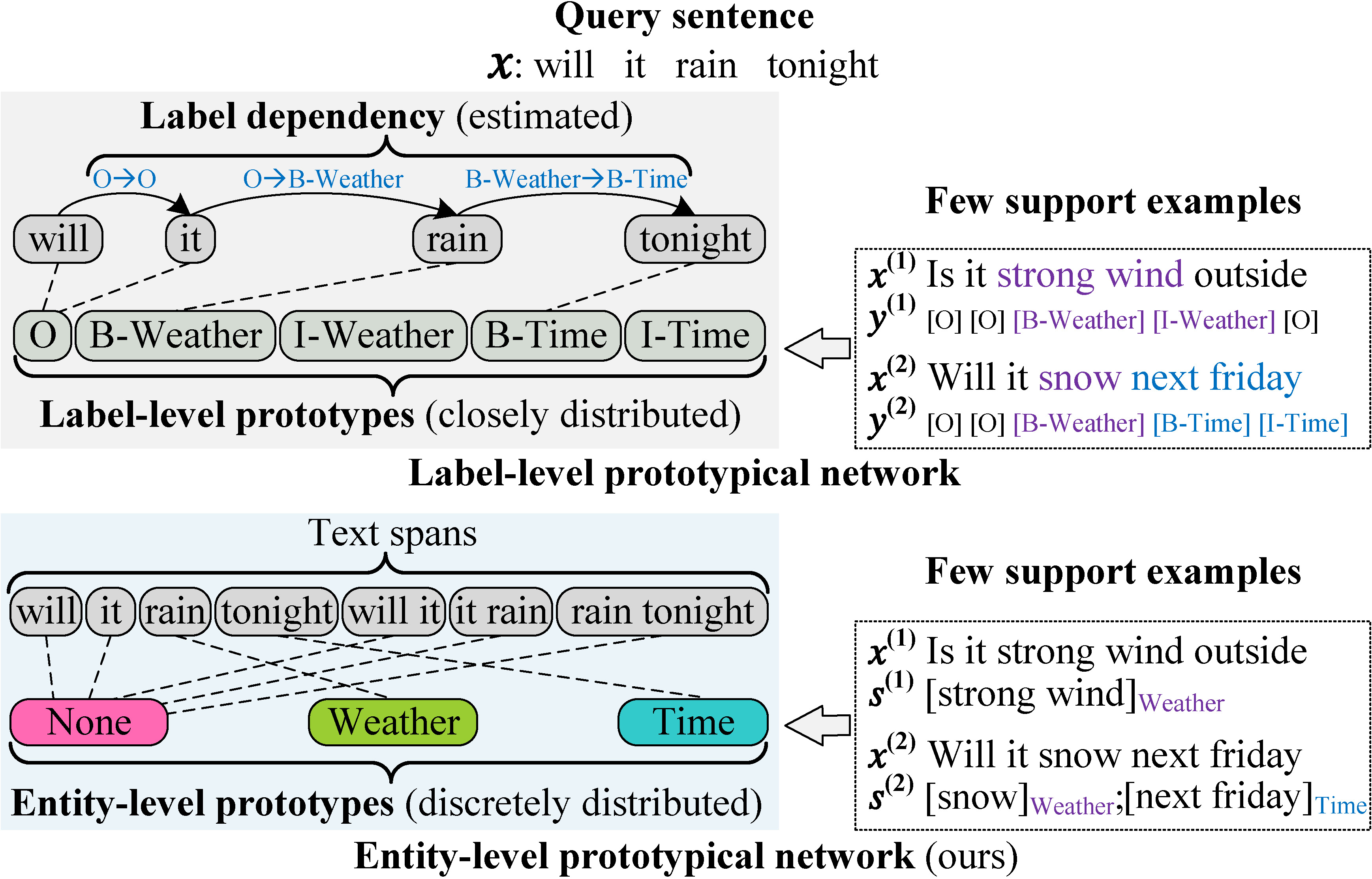
Figure 1: A comparison of token- and entity-level prototypical networks for few-shot NER, where the former builds prototypes for token labels and requires label dependency, while the latter builds prototypes for entity types and does not require label dependency. The dotted line denotes that the pair of token-prototype (or span-prototype) is the most similar. For clarity, we only list spans with lengths less than 2 and assume there are only 2 pre-defined entity types.

Previous few-shot NER models Fritzler et al. (2019); Hou et al. (2020); Yang and Katiyar (2020); Tong et al. (2021) generally formulate the task as a sequence labeling task and employ token-level prototypical networks Snell et al. (2017). These models first obtain token labels according to the most similar token-prototype pair and then obtain entities based on these labels, as Figure 1 shows. The sequence labeling benefits from label dependency Hou et al. (2020). However, when it comes to few-shot NER models, the label dependency is off the table, because a few labeled data is way insufficient to learn the reliable dependency, and the label sets could vary from domain to domain. To tackle this, some methods try to transfer roughly estimated dependency. Hou et al. Hou et al. (2020) first learn the abstract label transition probabilities in source domains and then copy them to target domains. As Figure 2a shows, the abstract O$\rightarrow$I probability is copied to three targets directly (the red lines). However, this makes the target probability sum of O$\rightarrow$(all labels) end up with 160%. To avoid the possible probability overflows, Yang and Katiyar Yang and Katiyar (2020) propose an even distribution method. As Figure 2b shows, the abstract O$\rightarrow$I probability is distributed evenly among the three targets (the green lines). However, this could lead to severe contradictions between the target probabilities and reality. For example, there are 4,983 DATE entities and only one EMAIL entity in the I2B2 test set, so the target probabilities of O$\rightarrow$I-DATE and O$\rightarrow$I-EMAIL should be clearly different. Consequently, the current dependency transferring may lead to misclassifications due to the roughly estimated target transition probabilities, even though it sheds some light on few-shot NER.

In addition, the majority of prototypical models for few-shot NER Huang et al. (2021); Li et al. (2020) obtain prototypes by averaging the embeddings of each class’s support examples, while Yoon et al. Yoon et al. (2019) and Hou et al. Hou et al. (2020) demonstrate that such prototypes distribute closely in the embedding space, thus often causing misclassifications.

In this paper, we aim to tackle the above issues inherent in token-level prototypical models. To this end, we propose EP-Net, an Entity-level Prototypical Network enhanced by dispersedly distributed prototypes, as Figure 1 shows. EP-Net builds entity-level prototypes and considers text spans as candidate entities. Thus it can determine whether a span is an entity directly according to the most similar prototype to the span. This also eliminates the need for the label dependency. For example, EP-Net determines the “rain” and “tonight” are two entities, and their types are the Weather and Time, respectively (Figure 1). In addition, to distribute these prototypes dispersedly, EP-Net trains them using a distance-based loss from scratch. And EP-Net aligns spans and prototypes in the same embedding space by utilizing a deep neural network to map span representations to the embedding spaces of prototypes.

In essence, EP-Net is a span-based model. Several span-based models Li et al. (2021); Fu et al. (2021); Yu et al. (2022) have been proposed for the supervised NER task. Our EP-Net differs from these models in two ways: (1) The EP-Net obtains entities based on the span-prototype similarity, while these models do so by classifying span representations. (2) The EP-Net works effectively with few labeled examples, whereas these models need a large number of labeled examples to guarantee good performance.

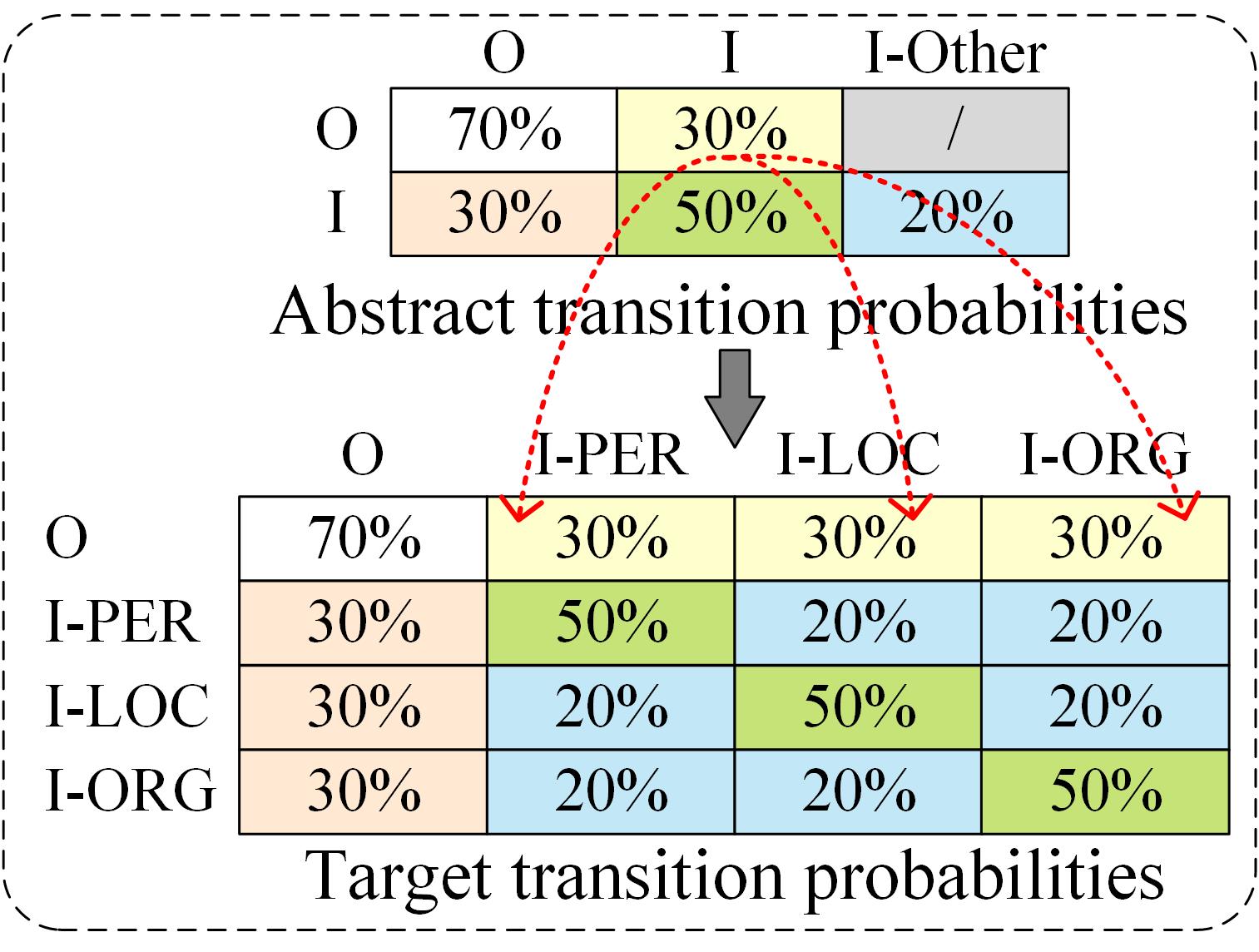
(a) Copying method

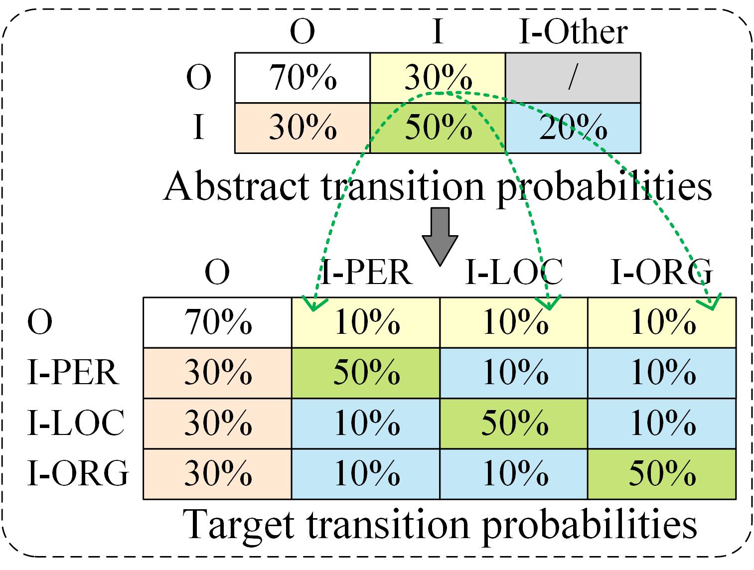
(b) Even distribution method

Figure 2: Methods of transferring estimated label dependency. In each method, the abstracts and corresponding targets are displayed in the same color. Method (a) copies the abstracts to the targets, whereas method (b) distributes them equally to the targets.

We evaluate our EP-Net on the tag set extension and domain transfer tasks, as well as the Few-NERD settings. Experimental results demonstrate that EP-Net consistently achieves new state-of-the-art overall performance. Qualitative analyses ($\S$5.5-5.6) and ablation studies ($\S$5.7) further validate the effectiveness of EP-Net.

In summary, we conclude the contributions as follows: (1) As far as we know, we are among the first to propose an entity-level prototypical network for few-shot NER. (2) We propose a prototype training strategy to augment the prototypical network with dispersedly distributed prototypes. (3) Our model achieves the current best overall performance on two evaluation tasks and the Few-NERD.

2 Related Work

Meta Learning. Meta learning aims to learn a general model that enables us to adapt to new tasks rapidly based on a few labeled examples Li et al. (2020). One of the most typical metric learning methods is the prototypical network Snell et al. (2017), which learns a prototype for each class and classifies an item based on item-prototype similarities. Metric learning has been widely investigated for NLP tasks, such as text classification Sun et al. (2019); Geng et al. (2019); Bao et al. (2020), relation classification Lv et al. (2019); Gao et al. (2020) and NER Huang et al. (2021). However, these methods use the prototypes obtained by averaging the embeddings of support examples for each class, which are closely distributed. In contrast, our model uses dispersedly distributed prototypes obtained by supervised prototype training.

Few-shot NER. Previous few-shot NER models Li et al. (2020); Tong et al. (2021) generally formulate the task as a sequence labeling task and propose to use the token-level prototypical network. Thus these models call for label dependency to guarantee good performance. However, it is hard to obtain exact dependency since the label sets vary greatly across domains. As an alternative, Hou et al. Hou et al. (2020) propose to transfer estimated dependency. They copy the learned abstract dependency from source to target domains, but the target dependency contradicts the probability definition. Yang and Katiyar Yang and Katiyar (2020) propose StructShot, which improves the above dependency transferring by equally distributing the abstract dependency to target domains, whereas the target dependency contradicts the reality. Das et al. Das et al. (2022) introduce Contrastive Learning to the StructShot, which inherits the estimated dependency transferring. We demonstrate that the roughly estimated dependency may harm model performance. In addition, prompt-based models Cui et al. (2021); Sun et al. (2021); Gu et al. (2022); Cui et al. (2022); Ding et al. (2022) have been widely researched for this task recently, but the model performance heavily relies on the chosen prompts. Current with our work, Wang et al. Wang et al. (2022) also propose a span-level prototypical network to bypass label dependency, but their work is still hampered by closely distributed prototypes. In contrast, our model constructs dispersedly distributed entity-level prototypes, thus avoiding the roughly estimated label dependency and closely distributed prototypes.

3 Task Formulation and Setup

In this section, we formally define the task and then introduce the standard evaluation setup.

3.1 Few-shot NER

We define an unstructured sentence as a token sequence $\mathcal{X}$ $=$ $(x_{1},x_{2},…,x_{n})$, and define entities annotated in $\mathcal{X}$ as ${\mathcal{E}}=[(e^{(1)},t^{(1)}),...,(e^{(k)},t^{(k)})]$, where $e^{(i)}$ and $t^{(i)}$ denote entity text and entity type, respectively. A domain $\mathcal{D}=\{(\mathcal{X}^{(i)},\mathcal{E}^{(i)})\}_{i=1}^{N_{\mathcal{D}}}$ is a set of ($\mathcal{X},\mathcal{E}$) pairs, and each $\mathcal{D}$ has a domain-specific entity type set $\mathcal{T}_{\mathcal{D}}=\{{t}_{i}\}^{N}_{i=1}$, and $N$ is various across domains.

We achieve the few-shot task through three steps: Train, Adapt and Recognize. We first train EP-Net with the data of source domains $\{\mathcal{D}_{1},\mathcal{D}_{2},...\}$. Then we then adapt the trained EP-Net to target domains {$\mathcal{D}\textquoteright_{1},\mathcal{D}\textquoteright_{2},…$} by fine-tuning it on support sets sampled from target domains. Finally, we recognize entities of query sets using the domain-adapted EP-Net. We formulate a support set as $\mathcal{S}$$=$$\{(\mathcal{X}^{(i)},\mathcal{E}^{(i)})\}_{i=1}^{N_{\mathcal{S}}}$, where $\mathcal{S}$ usually includes a few labeled examples ($K$-shot) of each entity type. For a target domain, we formally define the $K$-shot NER as follows: given a sentence $\mathcal{X}$ and a $K$-shot support set, find the best entity set ${\mathcal{E}}$ for $\mathcal{X}$.

3.2 The Standard Evaluation Setup

To facilitate meaningful comparisons of results for future research, Yang and Katiyar Yang and Katiyar (2020) propose a standard evaluation setup. The setup consists of the query set and support set constructions.

3.2.1 Query Set Construction

They argue that traditional construction methods sample different entity classes equally without considering entity distributions. For example, the I2B2 test set contains 4,983 DATE entities, while it only contains one EMAIL entity. Thus they propose to use the original test sets of standard NER datasets as the query sets, thus improving the reproducibility of future studies.

3.2.2 Support Set Construction

To construct support sets, they propose a Greedy Sampling algorithm to sample sentences from the dev sets of standard NER datasets. In particular, the algorithm samples sentences for entity classes in increasing order of their frequencies. We present the algorithm in Appendix A.

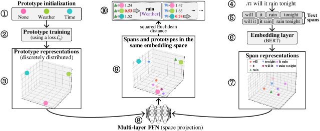
Figure 3: The architecture of EP-Net. As an example, we use the sentence in Figure 1 and 3-dimensional embedding spaces. EP-Net first initializes entity-level prototypes for entity types (①). Then it trains the prototypes with a distance-based loss $\mathcal{L}_{d}$ (②), distributing them dispersedly in embedding space (③). Next, given a sentence $\mathcal{X}$ (④), EP-Net first obtains text spans (⑤) and then uses BERT (⑥) to generate span representations (⑦). Fourth, EP-Net uses the space projdection (⑧) to align spans and prototypes in the same embedding space (⑨). Finally, EP-Net calculates span-prototype similarities measured by the squared Euclidean distance. The shorter the distance, the better the similarity. EP-Net classifies entities based on the best similarity, e.g., classifying the “rain” into the Weather type (⑩).

4 Model

In this section, we first provide an overview of EP-Net in $\S$4.1, and then illustrate the model initializations in $\S$4.2 and discuss the model in $\S$4.3.

4.1 EP-Net

Figure 3 shows the overall architecture of EP-Net. Given a domain $\mathcal{D}$$=$$\{(\mathcal{X}^{(i)},\mathcal{E}^{(i)})\}_{i=1}^{N_{\mathcal{D}}}$ and its entity type set $\mathcal{T}_{\mathcal{D}}=\{t_{i}\}_{i=1}^{N}$, we first initialize an entity-level prototype for each $t_{i}$ (Figure 3-①).

$$\boldsymbol{\it{\Phi}}=\{\boldsymbol{\phi}_{0},\boldsymbol{\phi}_{1},\boldsymbol{\phi}_{2},...,\boldsymbol{\phi}_{N}\},$$ (1)

where $\boldsymbol{\it{\Phi}}\in\mathbb{R}^{(N{+}1)*{d_{1}}}$, and $d_{1}$ is the dimension of prototype representation. $\boldsymbol{\phi}_{0}$ is the prototype of the None type, and $\boldsymbol{\phi}_{i}\ (i>0)$ is the prototype of $t_{i}$.

We design a distance-based loss $\mathcal{L}_{d}$ to supervise the prototype training (Figure 3-②), aiming to distribute these prototypes dispersedly in the embedding space (Figure 3-③). We argue that the prototypes should be dispersedly distributed in an appropriate-sized embedding space, neither too large nor too small ($\S$5.5). Thus we first set a threshold $\tau$ to limit the averaged prototype distance. Then we calculate the squared Euclidean distance between any two prototypes and obtain the averaged prototype distance (denoted as $Euc(\boldsymbol{\it{\Phi}})$). Next, we construct the $\mathcal{L}_{d}$ as follows.

$$\psi =\left\{\begin{array}[]{rcl}\leavevmode\resizebox{103.34666pt}{}{$Euc(\boldsymbol{\it{\Phi}})-\tau$}&{\textrm{if}}\ \ \ \leavevmode\resizebox{103.34666pt}{}{$Euc(\boldsymbol{\it{\Phi}})\geq\tau$,}\\ \leavevmode\resizebox{103.34666pt}{}{$\tau-Euc(\boldsymbol{\it{\Phi}})$}&{\textrm{if}}\ \ \ \leavevmode\resizebox{103.34666pt}{}{$Euc(\boldsymbol{\it{\Phi}})<\tau$,}\end{array}\right.$$ (2d)

$$\mathcal{L}_{d} =\log(\psi+1).$$ (2e)

The training goal is to achieve $\psi\rightarrow 0^{+}$, which equals to ${(\psi+1)}\rightarrow 1^{+}$. Thus we design the $\log(\cdot)$ loss (Eq.2e), where the smaller the $\mathcal{L}_{d}$, the more the $(\psi+1)\rightarrow 1^{+}$.

Next, given a sentence $\mathcal{X}=\{x_{i}\}_{i=1}^{n}$ of the domain $\mathcal{D}$, we first obtain text spans (denoted as $s$, Figure 3-④⑤):

$$s=\{x_{i},x_{i+1},...,x_{i+j}\}\ \leavevmode\resizebox{187.89912pt}{}{$s.t.\ 1\leq i\leq i+j\leq n$,}$$ (3)

where the span length $j$+$1$ is limited by a threshold $\epsilon$: $j$+$1\leq\epsilon$. To obtain the span representation (Figure 3-⑥⑦), we first use BERT Devlin et al. (2019) to generate the embedding sequence of $\mathcal{X}$.

$$\textbf{\em H}_{\mathcal{X}}=\{\boldsymbol{h}_{1},\boldsymbol{h}_{2},…,\boldsymbol{h}_{n}\},$$ (4)

where $\textbf{\em H}_{\mathcal{X}}\in\mathbb{R}^{n*d_{2}}$, and $d_{2}$ is the BERT embedding dimension. $\boldsymbol{h}_{i}$ is the BERT embedding of $x_{i}$. We use $\textbf{\em H}_{s}$ to denote the BERT embedding sequence of span $s$.

$$\textbf{\em H}_{s}=\{\boldsymbol{h}_{i},\boldsymbol{h}_{i+1},…,\boldsymbol{h}_{i+j}\}.$$ (5)

We obtain the span representation (denoted as $\textbf{\em E}_{s}$) by concatenating the max-pooling of $\textbf{\em H}_{s}$ (denoted as $\tilde{\textbf{\em H}}_{s}$) and the span length embedding.

$$\tilde{\textbf{\em H}}_{s} =\leavevmode\resizebox{399.2946pt}{}{$[\max(\boldsymbol{h}_{i,1},...,\boldsymbol{h}_{i+j,1}),...,\max(\boldsymbol{h}_{i,d_{1}},...,\boldsymbol{h}_{i+j,d_{1}})]$,}$$ (6a)

$$\textbf{\em E}_{s} =[\tilde{\textbf{\em H}}_{s};\boldsymbol{w}_{j+1}],$$ (6b)

where $\tilde{\textbf{\em H}}_{s}\in\mathbb{R}^{d_{2}}$, $\textbf{\em E}_{s}\in\mathbb{R}^{d_{2}+d_{3}}$. $\boldsymbol{w}_{j+1}$ is the length embedding trained for spans with a length $j$+$1$ and $d_{3}$ is the embedding dimension. Due to the fact that $\textbf{\em E}_{s}$ and prototype representations ($\boldsymbol{\it{\Phi}}$) are not in the same embedding space, we project $\textbf{\em E}_{s}$ to the embedding space of $\boldsymbol{\it{\Phi}}$ using a multi-layer Feed Forward Network (FFN) and denote the aligned span representation as $\tilde{\textbf{\em E}}_{s}$ (Figure 3-⑧⑨).

$$\tilde{\textbf{\em E}}_{s}=\textbf{\em E}_{s}\textbf{\em W}+\textbf{\em b},$$ (7)

where $\tilde{\textbf{\em E}}_{s}\in\mathbb{R}^{d_{1}}$, W and b are FFN parameters. Next, for the span $s$, we calculate the similarity between it and each prototype ${\boldsymbol{\phi}_{i}}\in\boldsymbol{\it\Phi}$ using the squared Euclidean distance.

$$\textrm{sim}(s,{\boldsymbol{\phi}_{i}})_{i=0}^{N}=\sum_{j=1}^{d}(\tilde{\textbf{\em E}}_{s,j}-\boldsymbol{\phi}_{i,j})^{2}.$$ (8)

As a shorter distance denotes a better similarity, we classify entities based the shortest distance (Figure 3-⑩):

$${t}_{s}=\mathrm{arg}\ \underset{\boldsymbol{\phi}_{i}\in\boldsymbol{\it\Phi}}{\mathrm{min}}\ \textrm{sim}(s,{\boldsymbol{\it\phi_{i}}})_{i=0}^{N},$$ (9)

where ${t}_{s}\in\mathcal{T}_{\mathcal{D}}$ is the type classified for the span $s$.

To construct an entity classification loss, we first take the $-\textrm{sim}(s,{\boldsymbol{\phi}_{i}})_{i=0}^{N}$ as classification logits, thus the best similarity has the largest logit. We then normalize these logits using the softmax function. Finally, we construct a cross-entropy loss $\mathcal{L}_{s}$.

$$\boldsymbol{\hat{y}}_{s,i} =\frac{\exp^{-\textrm{sim}(s,\boldsymbol{\phi}_{i})}}{\sum_{j=0}^{N}{\exp^{-\textrm{sim}(s,\boldsymbol{\phi}_{j})}}},$$ (10a)

$$\mathcal{L}_{s} =-\frac{1}{M_{s}}\sum_{j=1}^{M_{s}}\sum_{i=0}^{N}{\boldsymbol{y}}^{j}_{{s,i}}\log\hat{\boldsymbol{y}}^{j}_{{s,i}},$$ (10b)

where $\{\boldsymbol{{y}}_{{s}},\boldsymbol{{\hat{y}}}_{{s}}\}\in\mathbb{R}^{N+1}$, and $\boldsymbol{{y}}_{{s}}$ is the one-hot vector of the gold type for the span ${{s}}$. ${M_{s}}$ is the number of span instances.

During model training, we optimize model parameters by minimizing the following joint loss.

$$\mathcal{L}(\it{W};{\theta})=\mathcal{L}_{d}+\mathcal{L}_{s}.$$ (11)

4.2 Initializations

4.2.1 Train Initialization

In the Train step, given a source domain $\mathcal{D}$ with an entity type set $\mathcal{T}_{\mathcal{D}}$$=$$\{{t}_{i}\}^{N}_{i=1}$, we randomly initialize the entity-level prototypes $\boldsymbol{\it{\Phi}}=\{\boldsymbol{\phi}_{i}\}_{i=0}^{N}$.We assign $\boldsymbol{\phi}_{0}$ to the None type and $\boldsymbol{\phi}_{i}$ to $t_{i}$. To guarantee that we can adapt EP-Net to target domains that have more types than the domain $\mathcal{D}$, we actually initialize $\boldsymbol{\it{\Phi}}=\{\boldsymbol{\phi}_{i}\}_{i=0}^{100}$, where EP-Net can be adapted to any target domains with entity types less than 100. Moreover, the $N$ can be set to an even larger value if necessary. By doing so, the prototypes $\{\boldsymbol{\phi}_{i}\}_{i=N+1}^{100}$ are unassigned, but we can still distribute them dispersedly through training them using the loss $\mathcal{L}_{d}$ ($\S$5.6). We use the bert-base-cased model in the embedding Layer.

4.2.2 Adapt and Recognize Initializations

In the Adapt step, given a target domain $\mathcal{D^{\prime}}$ with an entity type set $\mathcal{T}_{\mathcal{D}^{\prime}}$$=$$\{{{t}^{\prime}_{i}}\}^{N^{\prime}}_{i=1}$ and the EP-Net trained in the Train step, we first assign a prototype of the trained $\boldsymbol{\it{\Phi}}=\{\boldsymbol{\phi}_{i}\}_{i=0}^{100}$ to each $t^{\prime}_{i}$. In particular, we assign $\boldsymbol{\phi}_{0}$ to the None type. And if there are types that are overlapped between $\mathcal{T}_{\mathcal{D}}$ and $\mathcal{T}_{\mathcal{D^{\prime}}}$ (i.e., $\mathcal{T}_{\mathcal{D}}\cap\mathcal{T}_{\mathcal{D^{\prime}}}\neq\varnothing$), for each overlapped type, we reuse the prototype assigned in the Train step. For other types in $\mathcal{T}_{\mathcal{D^{\prime}}}$, we randomly assign an unassigned prototype in $\boldsymbol{\it{\Phi}}$ to it, and we first choose the prototype that is ever assigned in the Train step. Then, we adapt EP-Net to the domain $\mathcal{D}^{\prime}$ by fine-tuning it on support sets sampled from $\mathcal{D^{\prime}}$.

However, Fine-tuning the model with small support sets runs the risk of overfitting. To avoid this, we propose to use the following strategies: (1) We freeze the BERT and solely fine-tune the assigned prototypes and the multi-layer FFN. (2) We use an early stopping criterion, where we continue fine-tuning our model until the loss starts to increase. (3) We set upper limits for fine-tuning steps, where the model will stop when reaching the limits even though the loss continues decreasing. With the above strategies, we demonstrate that only a few fine-tuning steps on these examples can make rapid progress without overfitting.

In the Recognize step, we use the domain-adapted EP-Net to recognize entities in the query set of $\mathcal{D^{\prime}}$ directly.

4.3 Model Discussion

In the Train step, the randomly initialized prototypes cannot represent entity types at first. Through the joint model training with the $\mathcal{L}(\it{W};{\theta})$, EP-Net establishes correlations between entity types and their assigned prototypes. Moreover, the multi-layer FFN can also be trained to cluster similar spans around related prototypes in the embedding space. As Figure 3-⑨ shows, the “rain” is mapped to be closer to the Weather than other prototypes.

To precisely simulate the few-shot scenario, we are not permitted to count the entity length of target domains. Thus we set the span length threshold $\epsilon$ to an empirical value of 10 based on source domains. For example, 99.89% of the entities in the OntoNotes have lengths under 10.

We propose a heuristic method for removing overlapped entities classified by EP-Net. Specifically, we keep the one with the best span-prototype similarity of those overlapped entities and drop the others.

Concurrently, Wang et al. Wang et al. (2022) propose a span-level model – ESD. We summarize how our EP-Net differs from the ESD as follows: (1) Our EP-Net fine-tunes on support sets while the ESD solely uses them for similarity calculation without fine-tuning. Ma et al. Ma et al. (2022) claim that the fine-tuning method is far more effective in using the limited information in support sets. (2) The ESD obtains class prototypes with embeddings of the same classes in support sets, thus suffering from closely distributed prototypes Hou et al. (2020). By contrast, our EP-Net avoids this by training dispersedly distributed prototypes from scratch.

Model	Tag Set Extension				Domain Transfer				Few-NERD
	Group A	Group B	Group C	Avg.	I2B2	CoNLL	WNUT	Avg.	Intra	Inter	Avg.
ProtoNet	18.7$\pm$4.7	24.4$\pm$8.9	18.3$\pm$6.9	20.5	7.6$\pm$3.5	53.0$\pm$7.2	14.8$\pm$4.9	25.1	18.6$\pm$7.2	25.3$\pm$8.8
ProtoNet+P&D	18.5$\pm$4.4	24.8$\pm$9.3	20.7$\pm$8.4	21.3	7.9$\pm$3.2	56.0$\pm$7.3	18.8$\pm$5.3	27.6	19.4$\pm$5.6	26.2$\pm$4.2	22.8
NNShot	27.2$\pm$3.5	32.5$\pm$14.4	23.8$\pm$10.2	25.7	16.6$\pm$2.1	61.3$\pm$11.5	21.7$\pm$6.3	33.2	20.1$\pm$8.5	25.7$\pm$7.7	22.9
StructShot	27.5$\pm$4.1	32.4$\pm$14.7	23.8$\pm$10.2	27.9	22.1$\pm$3.0	62.3$\pm$11.4	25.3$\pm$5.3	36.6	20.3$\pm$4.3	26.7$\pm$5.6	23.5
CONTaiNER	32.4$\pm$5.1	30.9$\pm$11.6	33.0$\pm$12.8	32.1	21.5$\pm$1.7	61.2$\pm$10.7	27.5$\pm$1.9	36.7	22.4$\pm$5.4	28.4$\pm$4.3	25.4
EP-Net (ours)	38.4$\pm$4.5	42.3$\pm$10.8	36.7$\pm$9.5	39.1	27.5$\pm$4.6	64.8$\pm$10.4	32.3$\pm$4.8	41.5	25.8$\pm$5.1	30.9$\pm$4.9	28.4

Table 1: F1 scores of 1-shot experiments. We report the mean and standard deviations of F1 scores.

Model	Tag Set Extension				Domain Transfer				Few-NERD
	Group A	Group B	Group C	Avg.	I2B2	CoNLL	WNUT	Avg.	Intra	Inter	Avg.
ProtoNet	27.1$\pm$2.4	38.0$\pm$5.9	38.4$\pm$3.3	34.5	10.3$\pm$0.4	65.9$\pm$1.6	19.8$\pm$5.0	32.0	33.2$\pm$6.4	31.7$\pm$5.9
ProtoNet+P&D	29.8$\pm$2.8	41.0$\pm$6.5	38.5$\pm$3.3	36.4	10.1$\pm$0.9	67.1$\pm$1.6	23.8$\pm$3.9	33.6	26.4$\pm$3.8	28.7$\pm$7.2	27.6
NNShot	44.7$\pm$2.3	53.9$\pm$7.8	53.0$\pm$2.3	50.5	23.7$\pm$1.3	74.3$\pm$2.4	23.9$\pm$5.0	40.7	29.6$\pm$5.3	33.9$\pm$5.1	31.8
StructShot	47.4$\pm$3.2	57.1$\pm$8.6	54.2$\pm$2.5	52.9	31.8$\pm$1.8	75.2$\pm$2.3	27.2$\pm$6.7	44.7	31.2$\pm$4.4	35.7$\pm$3.8	33.5
CONTaiNER	51.2$\pm$6.0	56.0$\pm$6.2	61.2$\pm$2.7	56.2	36.7$\pm$2.1	75.8$\pm$2.7	32.5$\pm$3.8	48.3	33.1$\pm$4.6	$38.4\pm$4.4	35.8
EP-Net (ours)	55.5$\pm$3.2	64.8$\pm$4.8	52.7$\pm$2.2	57.7	44.9$\pm$2.7	78.8$\pm$2.7	38.4$\pm$5.2	54.0	36.4$\pm$4.6	41.4$\pm$3.6	38.9

Table 2: F1 scores of 5-shot experiments. We report the mean and standard deviations of F1 scores.

5 Experiments

5.1 Evaluation Tasks

We evaluate EP-Net on two evaluation tasks and the Few-NERD settings using 1- and 5-shot settings. Limited by space, we solely report the key points here and discuss more details in Appendix B.

Tag Set Extension. This task aims to evaluate models for recognizing new types of entities in existing domains. Yang and Katiyar Yang and Katiyar (2020) divide the 18 entity types of the OntoNotes Ralph et al. (2013) into three target sets, i.e., Group A, B and C, to simulate this scenario. Models are evaluated on one target set while being trained on the others.

Domain Transfer. This task aims to evaluate models for adapting to a different domain. Yang and Katiyar Yang and Katiyar (2020) propose to use the general domain as the source domain and test model on medical, news, and social domains.

Few-NERD Settings. Few-NERD Ning et al. (2021) is a large-scale dataset for few-shot NER. It consists of two different settings: Intra and Inter. The Intra divides the train/dev/test according to coarse-grained types. The Inter divides the train/dev/test according to fine-grained types. Thus the coarse-grained entity types are shared. The Intra is more challenging as the restrictions of sharing coarse-grained types.

5.2 Datasets and Baselines

For a fair comparison, we use the same datasets and baselines reported in Yang and Katiyar (2020); Ning et al. (2021); Das et al. (2022). Specifically, we use OntoNotes (general domain), CoNLL 2003 Tjong Kim Sang and De Meulder (2003) (news domain), I2B2 2014 Stubbs and Özlem Uzuner (2015) (medical domain) and WNUT 2017 Derczynski et al. (2017) (social domain) for the tag set extension and domain transfer tasks.

We compare the performance of EP-Net with previous best models, including: Prototypical Network (ProtoNet) Snell et al. (2017), ProtoNet+P&D Hou et al. (2020) , NNShot and StructShot Yang and Katiyar (2020) and CONTaiNER Das et al. (2022). We represent more baseline details in Appendix C.

5.3 Implementation Details

In all experiments, we optimize EP-Net using AdamW with a learning rate of 5$e$-5 and set $d_{1}$ and $d_{3}$ to 512 and 25, respectively. $d_{2}$ is 768 when using the BERT base model. We set 3 layers for the multi-layer FFN, the distance threshold $\tau$ to 2, and the train batch size to 2 and 8 in 1- and 5-shot experiments, respectively. We set the distance threshold $\tau$ to 2 and 3 for 1- and 5-shot experiments, respectively. Moreover, we investigate the model performance against different $\tau$ values in Appendix D. Following supervised span-based work Ji et al. (2020), we sample spans of the None type during model training and set the sampled count to 20 and 40 in 1- and 5-shot experiments, respectively. Following Yang and Katiyar (2020); Das et al. (2022), we sample 5 support sets and report the mean and standard deviation of the F1 scores in each experiment.

5.4 Main Results

We report experimental results for 1- and 5-shot settings in Table 1 and Table 2, respectively. We have the following observations.

(1) In terms of the overall metric (i.e., Avg.), EP-Net consistently outperforms the listed baselines on the two tasks and Few-NERD, delivering +1.5% to +7.0% averaged F1 gains. Moreover, EP-Net improves up to +11.4% F1 scores on 1-shot Group B. We attribute these gains to the advantages of the proposed entity-level prototypical network.

(2) On the 5-shot Group C, EP-Net is inferior to CONTaiNER by 8.5% F1 scores. Detailed error analysis indicates that the group’s DATE type should bear the primary responsibility. Of the 4,178 entities in the test set, 1,536 are DATE entities, in which there are up to 429 different expressions, such as “week”, “this week”, ”last week”, “2 weeks”, “2 - week” etc. However, the 5-shot setting solely enables us to sample very few various expressions, leading to the poor performance in DATE entities. For example, if a support set solely samples the “week”, it is hard for EP-Net to recognize entities like “this week” and “last week”.

In addition, we conduct episode evaluations on Few-NERD and report the results in Appendix E.

5.5 Visualization

We use the 1-shot Group A experiment to investigate prototype distributions. Specifically, in the Train step we initialize the prototype set $\boldsymbol{\it{\Phi}}=\{\boldsymbol{\phi}\}_{i=0}^{100}$ and assign $\{\boldsymbol{\phi}\}_{i=0}^{12}$ to the None type and the 12 pre-defined entity types of the source domain. In the Adapt step, we assign $\{\boldsymbol{\phi}\}_{i=0}^{6}$ to the None type and the 6 pre-defined entity types of the Group A.

We report the visualization results in Figure 4. From Figure 4b, we observe that all prototypes are dispersedly distributed because the Euclidean distance between any two prototypes is approximate 2. Therefore, we conclude that EP-Net can distribute the prototypes dispersedly through the prototype training. From Figure 4a, we see that the distances between the None type and other assigned prototypes are generally larger than other distances. We attribute it to the fact that the None type does not represent any unified semantic meaning, thus the None spans actually correspond to a variety of semantic spaces, requiring the None prototype to keep away from other prototypes to alleviate the misclassification problem.

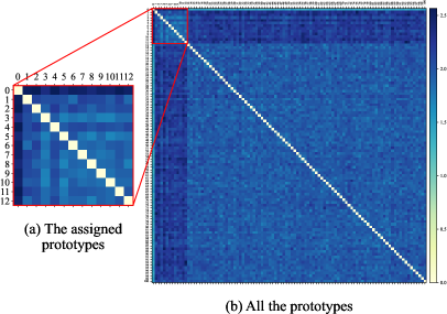
Figure 4: Heat maps of prototype distributions in the embedding space, which are measured by the squared Euclidean distance. In the (b), we show the distributions of all the prototypes $\boldsymbol{\it{\Phi}}=\{\boldsymbol{\phi}\}_{i=0}^{100}$. In the (a), we amplify the distributions of the 13 assigned prototypes $\{\boldsymbol{\phi}\}_{i=0}^{12}$. The darker the color, the larger the distance.

Moreover, we realize another entity-level prototypical network with conventional prototypes, and refer to it as CP-Net. We do not train the conventional prototypes with the loss $\mathcal{L}_{d}$ but fine-tune it during the model training. We report more details of CP-Net in Appendix F.

We visualize the distributions of our prototypes and conventional prototypes in Figure 5. To be specific, we use prototypes obtained in the Recognized step of both models. We observe that: (1) Our prototypes are distributed much more dispersedly than the conventional prototypes. (2) Our None prototype is more distant from other prototypes, whereas the conventional None prototype stays close to other conventional prototypes. These results indicate that our prototypes enable us to alleviate the misclassifications caused by closely distributed prototypes.

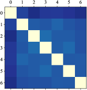
(a) Our prototypes

(b) Conventional prototypes

Figure 5: Heat maps of prototype distributions of our prototypes and conventional prototypes.

5.6 How does the Dispersedly Distributed Prototyes Enhance the EP-Net?

We run the 1-shot Group A experiment with EP-Net and CP-Net to conduct the investigation. We first compare the F1 scores of the two models. The results show our EP-Net outperforms CP-Net by +9.6% F1 scores, verifying the effectiveness of the dispersedly distributed prototypes.

In addition, we use t-SNE Van der Maaten and Hinton (2008) to reduce the dimension of span representations obtained in the Recognize step of EP-Net and CP-Net and visualize these representations in Figure 6. We can see that our EP-Net clusters span representations of the same entity class while dispersing span representations of different entity classes obviously, which we attribute to the usage of dispersedly distributed prototypes. Based on the above fact, we conclude that our EP-Net can greatly alleviate the misclassifications caused by closely distributed prototypes.

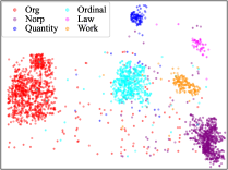
(a) EP-Net

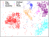
(b) CP-Net

Figure 6: t-SNE visualization of span representations of EP-Net and CP-Net. We obtain these representations in the Recognize step of both models. Since there are too many None spans (890,000+), we do not show their visualizations in the figure.

5.7 Ablation Study

We conduct ablation studies to investigate the significance of model components and report the results in Table 3. Specifically, (1) In the “- Entity-level prototype”, we ablate the entity-level prototypes and use token-level prototypes instead. Moreover, we use the copying method (Figure 2) to transfer the label dependency. The ablation results show that the F1 scores drop from 5.1% to 7.2%, validating the advantages of entity-level prototypes. (2) In the “- Prototype training”, we remove the loss $\mathcal{L}_{d}$ from the $\mathcal{L}(\it{W};{\theta})$, thus the prototypes are not trained being dispersedly distributed. The decreasing F1 scores (5.8% to 11.8%) demonstrate that EP-Net significantly benefits from the dispersedly distributed prototypes. (3) In the “-Euclidean distance”, we use the cosine similarity to measure span-prototype similarities instead. We see that the Euclidean similarity consistently surpasses the cosine similarity, revealing that a proper measure is vital to guarantee good performance, which is consistent with the conclusion in Snell et al. (2017).

Model	Group A (F1)	I2B2 (F1)	Intra (F1)	Inter (F1)
EP-Net	38.4	27.5	25.8	30.9
- Entity-level prototype	31.6	22.4	18.6	25.1
- Prototype training	30.3	19.8	20.0	19.1
- Euclidean distance	33.4	25.2	21.6	27.3

Table 3: Ablation results under the 1-shot setting. We select one dataset for each of the two evaluation tasks, as well as the Intra and Inter of the Few-NERD.

6 Conclusion

In this paper, we propose an entity-level prototypical network for few-shot NER (EP-Net). And we augment EP-Net with dispersedly distributed prototypes. The entity-level prototypes enable EP-Net to avoid suffering from the roughly estimated label dependency brought by abstract dependency transferring. Moreover, EP-Net distributes the prototypes dispersedly via supervised prototype training and maps spans to the embedding space of the prototypes to eliminate the alignment biases. Experimental results on two evaluation tasks and the Few-NERD settings demonstrate that EP-Net beats the previously published models, creating new state-of-the-art overall performance. Extensive analyses further validate the model’s effectiveness.

Appendix

Appendix A The Greedy Sampling Algorithm

Algorithm 1: Greedy Sampling Algorithm

Require: shot $K$, dev set X of a domain $\mathcal{D}$ and its entity          type set ${\mathcal{T}}$      1: Sort types in $\mathcal{T}$ based on their frequencies in X      2: $\mathcal{S}$ $\leftarrow$ $\varnothing$   // Initialize the support set     3: {Counti $\leftarrow$ 0}          // Initialize the count of each type in $\mathcal{S}$     4: while $i$ < $\mid$${\mathcal{T}}$$\mid$ do     5:   while Counti < $K$ do     6:      Sample $(\mathcal{X},\mathcal{E})$ $\in$ $\mathbf{X}$    $s.t.$    ${\mathcal{T}}_{i}$ $\in$ $\mathcal{E}.type{\textsuperscript{1}}$              // Sample a sentence containing entities of $\mathcal{T}_{i}$              // type, w/o replacement     7:      $\mathcal{S}$ $\leftarrow$ $\mathcal{S}$ $\cup$ {$(\mathcal{X},\mathcal{E})$}     8:      update {Countj}  $\forall$ ${\mathcal{T}}_{j}$ $\in$ $\mathcal{E}.type$     9:   end while 10: end while 11: return $\mathcal{S}$

• $\mathcal{E}.type$ denotes the types of entities annotated in $\mathcal{E}$

Appendix B Details of the Evaluation Task

B.1 Tag Set Extension

The Group A, B, and C split from the OntoNotes dataset are as follows.

• Group A: {Org, Quantity, Ordinal, Norp, Work, Law}

• Group B: {Gpe, Cardinal, Percent, Time, Event, Language}

• Group C: {Person, Product, Money, Date, Loc, Fac}

In this task, we evaluate our EP-Net on each group while training our model on the other two groups. In each experiment, we modify the training set by replacing all entity types in the target type set with the None type. Hence, these target types are no longer observed during training. We use the modified training set for model training in the Train step. Similarly, we modify the dev and test sets to only include entity types contained in the target type set. We use the Greedy Sampling Algorithm to sample multiple support sets from the dev set for model adaption.

B.2 Domain Transfer

In this task, we train our EP-Net on the standard training set of the OntoNotes dataset and evaluate our model on the standard test sets of I2B2, CoNLL, and WNUT. In addition, we sample support sets for model adaption from the standard dev sets of the above three datasets.

B.3 Few-NERD Settings

FEW-NERD Ning et al. (2021) is the first dataset specially constructed for few-shot NER and is one of the largest human-annotated NER datasets. It consists of 8 coarse-grained entity types and 66 fine-grained entity types. The dataset contains two sub-sets, name Intra and Inter.

• In Intra, all the fine-grained entity types belonging to the coarse-grained People, MISC, Art, Product are assigned to the training set, and all the fine-grained entity types belonging to the coarse-grained Event, Building are assigned to the dev set, and all the fine-grained entity types belonging to the coarse-grained ORG, LOC are assigned to the test set. In this dataset, the training/dev/test sets share little knowledge, making it a difficult benchmark.

• In Inter, 60% of the 66 fine-grained types are assigned to the training set, 20% to the dev set, and 20% to the test set. The intuition of this dataset is to explore if the coarse information will affect the prediction of new entities.

We use the standard evaluation ($\S$3.2) and the episode evaluation to evaluate the performance of our EP-Net. For the standard evaluation, we conduct experiments on Intra and Inter, respectively. We first use the training set to train our EP-Net and then sample support sets from the test set for the model adaptation and evaluate our model on the remaining test set. For the episode evaluation, we use the exact evaluation setting proposed by Ning et al. (2021).

Appendix C Baseline Details

Following the established line of work Yang and Katiyar (2020); Das et al. (2022); Ning et al. (2021), we compare EP-Net with the following competitive models.

• Prototypical Network (ProtoNet) Snell et al. (2017) is a popular few-shot classification algorithm that has been adopted in most previously published token-level few-shot NER models.

• ProtoNet+P&D Hou et al. (2020) uses pair-wise embedding and collapsed dependency transfer mechanism in the token-level Prototypical Network, tackling challenges of similarity computation and transferring estimated label dependency across domains.

• NNShot Yang and Katiyar (2020) is a simple token-level nearest neighbor classification model. It simply computes a similarity score between a token in the query example and all tokens in the support set.

• StructShot Yang and Katiyar (2020) combines NNShot and Viterbi decoder and uses estimated label dependency across domains by first learning abstract label dependency and then distributing it evenly to target domains.

• CONTaiNER Das et al. (2022) introduces Contrast Learning to the StructShot. It models Gaussian embedding and optimizes inter token distribution distance, which aims to decrease the distance of token embeddings of similar entities while increasing the distance for dissimilar ones.

For a fair comparison, we use the results of the ProtoNet, ProtoNet+P&D, NNShot, and StructShot reported in Yang and Katiyar (2020), and the results of CONTaiNER reported in Das et al. (2022).

In addition, we run the ProtoNet, ProtoNet+P&D, NNShot, and StructShot on Few-NERD using the standard evaluation setup ($\S$3.2, B.3).

Appendix D Performance against Prototype Distance Threshold ($\tau$)

We conduct 1- and 5-shot experiments to explore the performance against different $\tau$ values. Since validation sets are unavailable in the few-shot scenario, we randomly sample 20% of the query sets for the explorations. We report the results in Figure 7, where we set the $\tau$ value from 1 to 10, respectively. We can observe that: (1) The F1 scores generally first increase and then decrease when the $\tau$ value consistently increases. (2) Except for the Group C and Intra, our EP-Net performs the best in the 1-shot experiments when setting the $\tau$ to 2. (3) Except for the Group A and Intra, our EP-Net performs the best in the 5-shot experiments when setting the $\tau$ to 3.

The above results validate our argument that the prototypes should be distributed in an appropriate-sized embedding space, neither too large nor too small ($\S$4.1). For simplicity, we set the $\tau$ to 2 and 3 in all the other 1- and 5-shot experiments, respectively.

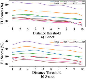
Figure 7: Performance comparisons of different prototype distance threshold ($\tau$) values in 1- and 5-shot experiments.

Appendix E Episode Evaluation on Few-NERD

We evaluate our EP-Net on Few-NERD with the episode evaluation setting and compare our model with previous state-of-the-art models, including ProtoBERT Ning et al. (2021), NNShot, StructShot, CONTaiNER, and ESD Wang et al. (2022). We would like to mention that the ESD is a concurrent span-based few-shot NER model to ours.

Model	1$\sim$2-shot			5$\sim$10-shot		Avg.
	5 way	10 way		5 way	10 way
ProtoBERT	23.45$\pm$0.92	19.76$\pm$0.59		41.93$\pm$0.55	34.61$\pm$0.59	29.94
NNShot	31.01$\pm$1.21	21.88$\pm$0.23		35.74$\pm$2.36	27.67$\pm$1.06	29.08
StructShot	35.92$\pm$0.69	25.38$\pm$0.84		38.83$\pm$1.72	26.39$\pm$2.59	31.63
ESD	41.44$\pm$1.16	32.29$\pm$1.10		50.68$\pm$0.94	42.92$\pm$0.75	41.83
CONTaiNER	40.43	33.84		53.70	47.49	43.87
EP-Net (Ours)	43.36$\pm$0.99	36.41$\pm$1.03		58.85$\pm$1.12	46.40$\pm$0.87	46.26

Table 4: Episode evaluation results (F1 scores) on the Intra dataset of Few-NERD. We report the mean and standard deviations of F1 scores.

Model	1$\sim$2-shot			5$\sim$10-shot		Avg.
	5 way	10 way		5 way	10 way
ProtoBERT	44.44$\pm$0.11	39.09$\pm$0.87		58.80$\pm$1.42	53.97$\pm$0.38	49.08
NNShot	54.29$\pm$0.40	46.98$\pm$1.96		50.56$\pm$3.33	50.00$\pm$0.36	50.46
StructShot	57.33$\pm$0.53	49.46$\pm$0.53		57.16$\pm$2.09	49.39$\pm$1.77	53.34
CONTaiNER	55.95	48.35		61.83	57.12	55.81
ESD	66.46$\pm$0.49	59.95$\pm$0.69		74.14$\pm$0.80	67.91$\pm$1.41	66.12
EP-Net (Ours)	62.49$\pm$0.36	54.39$\pm$0.78		65.24$\pm$ 0.64	62.37$\pm$1.27	61.12

Table 5: Episode evaluation results (F1 scores) on the Inter dataset of Few-NERD. We report the mean and standard deviations of F1 scores.

We report the results in Table 4 and Table 5, where we take the results of ProtoBERT, NNShot, and StructShot reported in Ning et al. (2021), and the results of CONTaiNER and ESD reported in their original papers. We can see that:

• On the Intra, our EP-Net consistently outperforms the best baseline (i.e., CONTaiNER) in terms of the Avg. metric, bringing +2.39% F1 gains. In addition, our EP-Net surpasses the concurrent ESD by +4.43% F1 scores.

• On the Inter, our EP-Net is inferior to ESD by a large margin (5.0%) in terms of the Avg. metric. However, our model consistently outperforms the other baselines, delivering up to +5.31% F1 scores compared to the CONTaiNER.

• Both our EP-Net and CONTaiNER outperform ESD in 1-shot experiments, but they are inferior to ESD in 5-shot experiments.

The above results demonstrate the effectiveness of the proposed EP-Net. And compared to ESD, our model is more efficient in the few-shot scenario when entities share less coarse-grained information (the Intra).

Compared to our simple concatenation method (Eq.6b) to obtain span representations, ESD proposes to use Inter Span Attention (ISA) and Cross Span Attention (CSA) to enhance the span representations. We believe that the ISA and CSA enable ESD to encode the shared coarse-grained information into span representations sufficiently, which helps ESD obtain the current state-of-the-art performance on the Inter dataset.

Appendix F CP-Net

We propose the CP-Net as a comparable model to our EP-Net. CP-Net is also an entity-level prototypical network, but it uses conventional prototypes obtained by averaging the embeddings of type’s examples. Similar to EP-Net, CP-Net also uses the BERT model as an embedding generator. In addition, it uses the sampling strategy discussed in $\S$5.3 to randomly sample None spans. CP-Net consists of two steps, namely Train and Recognize.

In the Train step, we train CP-Net with the source domain data. To be specific, we obtain the entity-level prototypes by averaging the embeddings of type’s examples in the training set. Moreover, we obtain span representations with the same method of EP-Net (Eq.3-7), as well as the method to calculate span-prototype similarity (Eq.8-9). During the model training, we use the training loss $\mathcal{L}_{s}$ (Eq.10b) to fine-tune the BERT model.

In the Recognize step, we use the fine-tuned BERT model as the embedding generator and obtain the entity-level prototypes by averaging the embeddings of each type’s examples in the support sets. Then we obtain the type of each span according to the best similarity between the span and the prototypes.

The CP-Net differs from our EP-Net in the following two ways.

• CP-Net uses conventional prototypes, and it does not train these prototypes during the model training. By contrast, our EP-Net trains prototypes from scratch with the distance based loss $\mathcal{L}_{d}$ (Eq.2e)

• CP-Net does not contain a domain adaption procedure, and it solely uses the support sets for similarity calculation. By contrast, our EP-Net contains a Adapt step for domain adaption and it uses the support sets for not only the similarity calculation but also the domain adaption.

References

- Bao et al. (2020) Yujia Bao, Menghua Wu, Shiyu Chang, and Regina Barzilay. 2020. Few-shot text classification with distributional signatures. In Proc. of ICLR.
- Cui et al. (2022) Ganqu Cui, Shengding Hu, Ning Ding, Longtao Huang, and Zhiyuan Liu. 2022. Prototypical verbalizer for prompt-based few-shot tuning. In Proc. of ACL.
- Cui et al. (2021) Leyang Cui, Yu Wu, Jian Liu, Sen Yang, and Yue Zhang. 2021. Template-based named entity recognition using BART. In Proc. of ACL.
- Das et al. (2022) Sarkar Snigdha Sarathi Das, Arzoo Katiyar, and Rui Zhang. 2022. Container: Few-shot named entity recognition via contrastive learning.
- Derczynski et al. (2017) Leon Derczynski, Eric Nichols, Marieke van Erp, and Nut Limsopatham. 2017. Results of the WNUT2017 shared task on novel and emerging entity recognition. In Proceedings of the 3rd Workshop on Noisy User-generated Text.
- Devlin et al. (2019) Jacob Devlin, Ming-Wei Chang, Kenton Lee, and Kristina Toutanova. 2019. BERT: Pre-training of deep bidirectional transformers for language understanding. In Proc. of ACL.
- Ding et al. (2022) Ning Ding, Shengding Hu, Weilin Zhao, Yulin Chen, Zhiyuan Liu, Hai-Tao Zheng, and Maosong Sun. 2022. Openprompt: An open-source framework for prompt-learning. In Proc. of ACL.
- Fritzler et al. (2019) Alexander Fritzler, Varvara Logacheva, and Maksim Kretov. 2019. Few-shot classification in named entity recognition task. In Proc. of SAC.
- Fu et al. (2021) Jinlan Fu, Xuanjing Huang, and Pengfei Liu. 2021. SpanNER: Named entity re-/recognition as span prediction. In Proc. of ACL.
- Gao et al. (2020) Tianyu Gao, Xu Han, Ruobing Xie, zhiyuan Liu, Fen Lin, Leyu Lin, , and Maosong Sun. 2020. Neural snowball for few-shot relation learning. In Proc. of AAAI.
- Geng et al. (2019) Ruiying Geng, Binhua Li, Yongbin Li, Xiaodan Zhu, Ping Jian, and Jian Sun. 2019. Induction networks for few-shot text classification. In Proc. of EMNLP.
- Gu et al. (2022) Yuxian Gu, Xu Han, Zhiyuan Liu, and Minlie Huang. 2022. Ppt: Pre-trained prompt tuning for few-shot learning. In Proc. of ACL.
- Hou et al. (2020) Yutai Hou, Wanxiang Che, Yongkui Lai, Zhihan Zhou, Han Liu, and Ting Liu. 2020. Few-shot slot tagging with collapsed dependency transfer and label-enhanced task-adaptive projection network. In Proc. of ACL.
- Huang et al. (2021) Jiaxin Huang, Chunyuan Li, Krishan Subudhi, Damien Jose, Weizhu Chen, Baolin Peng, Jianfeng Gao, and Jiawei Han. 2021. Few-shot named entity recognition: A comprehensive study. In Proc. of EMNLP.
- Ji et al. (2020) Bin Ji, Jie Yu, Shasha Li, Jun Ma, Qingbo Wu, Yusong Tan, and Huijun Liu. 2020. Span-based joint entity and relation extraction with attention-based span-specific and contextual semantic representations. In Proc. of COLING.
- Li et al. (2021) Fei Li, ZhiChao Lin, Meishan Zhang, and Donghong Ji. 2021. A span-based model for joint overlapped and discontinuous named entity recognition. In Proc. of ACL.
- Li et al. (2020) Jing Li, Billy Chiu, Shanshan Feng, and Hao Wang. 2020. Few-shot named entity recognition via meta-learning. IEEE Transactions on Knowledge and Data Engineering.
- Lv et al. (2019) Xin Lv, Yuxian Gu, Xu Han, Lei Hou, Juanzi Li, and Zhiyuan Liu. 2019. Adapting meta knowledge graph information for multi-hop reasoning over few-shot relations. In Proc. of EMNLP.
- Ma et al. (2022) Tingting Ma, Huiqiang Jiang, Qianhui Wu, Tiejun Zhao, and Chin-Yew Lin. 2022. Decomposed meta-learning for few-shot named entity recognition. In Proc. of ACL.
- Ning et al. (2021) Ding Ning, Guangwei Xu, Yulin Chen, Xiaobin Wang, Xu Han, Pengjun Xie, Haitao Zheng, and Zhiyuan Liu. 2021. Few-NERD: A few-shot named entity recognition dataset. In Proc. of ACL.
- Ralph et al. (2013) Weischedel Ralph, Martha Palmer, Mitchell Marcus, Eduard Hovy, Sameer Pradhan, Lance Ramshaw, and Nianwen Xue. 2013. Ontonotes release 5.0 ldc2013t19. In Linguistic Data Consortium.
- Snell et al. (2017) Jake Snell, Kevin Swersky, and Richard Zemel. 2017. Prototypical networks for few-shot learning. In Proc. of ICONIP.
- Stubbs and Özlem Uzuner (2015) Amber Stubbs and Özlem Uzuner. 2015. Annotating longitudinal clinical narratives for de-identification: The 2014 i2b2/uthealth corpus. Journal of Biomedical Informatics.
- Sun et al. (2019) Shengli Sun, Qingfeng Sun, Kevin Zhou, and Tengchao Lv. 2019. Hierarchical attention prototypical networks for few-shot text classification. In Proc. of EMNLP.
- Sun et al. (2021) Yi Sun, Yu Zheng, Chao Hao, and Hangping Qiu. 2021. NSP-BERT: A prompt-based zero-shot learner through an original pre-training task-next sentence prediction. CoRR.
- Tjong Kim Sang and De Meulder (2003) Erik F. Tjong Kim Sang and Fien De Meulder. 2003. Introduction to the CoNLL-2003 shared task: Language-independent named entity recognition. In Proc. of HLT-NAACL.
- Tong et al. (2021) Meihan Tong, Shuai Wang, Bin Xu, Yixin Cao, Minghui Liu, Lei Hou, and Juanzi Li. 2021. Learning from miscellaneous other-class words for few-shot named entity recognition. In ACL.
- Van der Maaten and Hinton (2008) Laurens Van der Maaten and Geoffrey Hinton. 2008. Visualizing data using t-sne. Journal of machine learning research, 9(11).
- Wang et al. (2022) Peiyi Wang, Runxin Xu, Tianyu Liu, Qingyu Zhou, Yunbo Cao, Baobao Chang, and Zhifang Sui. 2022. An enhanced span-based decomposition method for few-shot sequence labeling. In Proc. of NAACL.
- Yang and Katiyar (2020) Yi Yang and Arzoo Katiyar. 2020. Simple and effective few-shot named entity recognition with structured nearest neighbor learning. In Proc. of EMNLP.
- Yoon et al. (2019) Sung Whan Yoon, Jun Seo, and Jaekyun Moon. 2019. TapNet: Neural network augmented with task-adaptive projection for few-shot learning. In Proc. of ICML.
- Yu et al. (2022) Jie Yu, Bin Ji, Shasha Li, Jun Ma, Huijun Liu, and Hao Xu. 2022. S-ner: A concise and efficient span-based model for named entity recognition. Sensors, 22(8):2852.