Investigating the Impact of Model Width and Density on Generalization in Presence of Label Noise

Abstract

Increasing the size of overparameterized neural networks has been a key in achieving state-of-the-art performance. This is captured by the double descent phenomenon, where the test loss follows a decreasing-increasing-decreasing pattern as model width increases. However, the effect of label noise on the test loss curve has not been fully explored. In this work, we uncover an intriguing phenomenon where label noise leads to a final ascent in the originally observed double descent curve. Specifically, under a sufficiently large noise-to-sample-size ratio, optimal generalization is achieved at intermediate widths. Through theoretical analysis, we attribute this phenomenon to the shape transition of test loss variance induced by label noise. Furthermore, we extend the final ascent phenomenon to model density and provide the first theoretical characterization showing that reducing density by randomly dropping trainable parameters improves generalization under label noise. We also thoroughly examine the roles of regularization and sample size. Surprisingly, we find that larger $\ell_{2}$ regularization and robust learning methods against label noise exacerbate the final ascent. We confirm the validity of our findings through extensive experiments on ReLu networks trained on MNIST, ResNets trained on CIFAR-10/100, and InceptionResNet-v2 trained on Stanford Cars with real-world noisy labels.

1 Introduction

Training neural networks of ever-increasing size on large datasets has played a pivotal role in achieving state-of-the-art generalization performance across various tasks Devlin et al. (2018); Dosovitskiy et al. (2020); Brown et al. (2020); Radford et al. (2021). While large unlabeled data can often be easily collected, obtaining high-quality labels for these datasets is prohibitively expensive, leading to the use of labeling techniques, such as crowd-sourcing and automatic labeling, that introduce a significant amount of label noise Krishna et al. (2016). Unfortunately, the impact of label noise on the generalization behavior of neural networks in relation to model size has not been comprehensively examined.

Recent research has aimed to reconcile the generalization benefits of increasing the size of overparameterized neural networks with the classical bias-variance trade-off that advocates for intermediate model size. To this end, the double descent phenomenon Belkin et al. (2019); Spigler et al. (2019) has been proposed, suggesting that the test loss initially follows a U-shaped curve but then descends again once the model is overparameterized. The works of Yang et al. (2020); Adlam and Pennington (2020a) attribute this behavior to the combination of decreasing bias and the unimodal variance of the test loss with respect to model width. However, the effect of label noise on the double descent phenomenon has not been fully explored.

In this work, we reveal that label noise can significantly alter the shape of the loss curve. Our study uncovers an intriguing phenomenon, which we refer to as the final ascent. In a wide range of settings, label noise leads to an eventual ascent in the originally observed double descent loss curve. Through theoretical analysis, we show that this occurs because sufficiently large noise-to-sample size ratio transforms the variance of the test loss from unimodal to an increasing-decreasing-increasing shape. We also provide further insights into the final ascent phenomenon. Firstly, perhaps surprisingly, applying stronger $\ell_{2}$ regularization only exacerbates the phenomenon as it enables intermediate model sizes to achieve lower test loss. Secondly, increasing the sample size can alleviate the final ascent.

Furthermore, we add model density, defined as the fraction of parameters that are trainable, as a new dimension to the discussion on generalization. We provide the first theoretical characterization of final ascent with respect to model density, showing that optimal generalization is achieved by intermediate density under label noise. Additionally, we make two significant findings. Firstly, as density decreases, the optimal model width increases and achieves lower test loss, which highlights the advantage of wider but sparser models. Secondly, while reducing density has a similar effect to stronger $\ell_{2}$ regularization in theory, in practice, adjusting the density of neural networks achieves even lower density compared to adjusting the regularization.

We also empirically examine the final ascent phenomenon when models are trained with robust learning algorithms that are designed to counteract the effect of label noise. Our results demonstrate that, similar to the impact of $\ell_{2}$ regularization, state-of-the-art robust algorithms Liu et al. (2020); Li et al. (2020) amplify the final ascent phenomenon. This finding suggests that models with intermediate width or density can be even more beneficial when these algorithms are used, which is typically the case in practical scenarios.

Our findings are supported by extensive experiments. We confirm the validity of our results across various settings, including random feature regression, training two-layer networks on MNIST LeCun (1998), ResNetsHe et al. (2016) on CIFAR-10 and CIFAR-100Krizhevsky et al. (2009), and InceptionResNet-v2 Szegedy et al. (2017) on Stanford Cars dataset with real label noiseJiang et al. (2020). We provide an in-depth discussion of how different factors affect the final ascent phenomenon. Notably, the final ascent can even occur with as little as 20% label noise in some settings. In summary, our results underscore the significance of exercising caution while employing large models and the benefits of intermediate model width and density and provide valuable insights into the roles of regularization and sample size. Our comprehensive theoretical and empirical picture holds the potential to guide and inspire future research in this field.

2 Related Work

Double descent. Contrary to the classical learning theory that advocates for intermediate model size, recent works have shown that increasing the size of overparameterized neural networks only improves generalization Neyshabur et al. (2014). This is explained by the double descent phenomenon Belkin et al. (2019); Spigler et al. (2019), which posits that the test loss initially follows a U-shape and then descends again once the model is overparameterized. This phenomenon has been theoretically investigated in various regression settings, including one-layer linear (Belkin et al., 2020; Derezinski et al., 2020; Kuzborskij et al., 2021), random feature (Hastie et al., 2019; Mei and Montanari, 2019; Adlam and Pennington, 2020a; Yang et al., 2020; d’Ascoli et al., 2020), and NTK (Adlam and Pennington, 2020b) regressions. While the primary focus has been on the behavior of the test loss Hastie et al. (2019); Belkin et al. (2020); Derezinski et al. (2020); Adlam and Pennington (2020b), some works have decomposed it into bias and variance (Mei and Montanari, 2019; Yang et al., 2020), and a few have further decomposed the variance into multiple sources, including label noise (Adlam and Pennington, 2020a; d’Ascoli et al., 2020). However, the effect of label noise has mainly been analyzed in terms of how it exacerbates the peak of the double descent curve Adlam and Pennington (2020a); Nakkiran et al. (2021). In contrast, the novel contribution of this work is the discovery of the final ascent, which has not been previously revealed in the literature.

Neural network density. Frankle and Carbin (2018); Lee et al. (2018); Frankle et al. (2019); Wang et al. (2020); Frankle et al. (2020); Tanaka et al. (2020) proposed methods to reduce model density (pruning) for improved training and inference efficiency. Jin et al. (2022) empirically investigated the impact of density on generalization using a pruning technique Renda et al. (2020) involving training and rewinding. However, the effect of density as a factor of model size has remained poorly understood, as pruning techniques incorporate additional information from training, initialization, or gradients. In contrast, we randomly drop weights thus isolating the effect of model size from other factors. We provide theoretical analysis of random feature regression, complementing the empirical nature of the aforementioned works. Exploring the effects of specific pruning techniques on the final ascent phenomenon uncovered in this paper could be an interesting future work.

Robust methods. Extensive efforts have been made to develop methods that can learn robustly against noisy labels Zhang and Sabuncu (2018); Jiang et al. (2018); Han et al. (2018); Mirzasoleiman et al. (2020); Liu et al. (2020); Li et al. (2020). These methods can be viewed as a form of regularization that helps alleviate the impact of label noise. In this work, we show that final ascent is exacerbated when robust methods are employed. Specifically, reducing the model width or density can yield even greater benefits when training with robust methods.

3 Theoretical Analysis of Random Feature Ridge Regression

In this section, we theoretically analyze the effect of label noise on the the test loss curve of a linear neural network with a random first layer. Random feature regression has been the go-to model in the literature for studying the double descent phenomenon Hastie et al. (2019); Mei and Montanari (2019); Yang et al. (2020); Adlam and Pennington (2020a); d’Ascoli et al. (2020), owing to its theoretical tractability. We note that studying regression tasks has uncovered fundamental insights Hastie et al. (2019); Mei and Montanari (2019); Advani et al. (2020); Bartlett et al. (2020) into the generalization behavior of neural networks applied to classification tasks.

We start by showing that sufficiently large noise-to-sample-size ratio introduces a final ascent to the loss curve, and explain it through the shape of variance. Then, we provide the first theoretical study on the effect of model density, showing that reducing the density of a wide model can improve its performance under label noise. We will confirm the validity of our results on various classification tasks with neural networks in Section 4.

3.1 Effect of Width: the Final Ascent

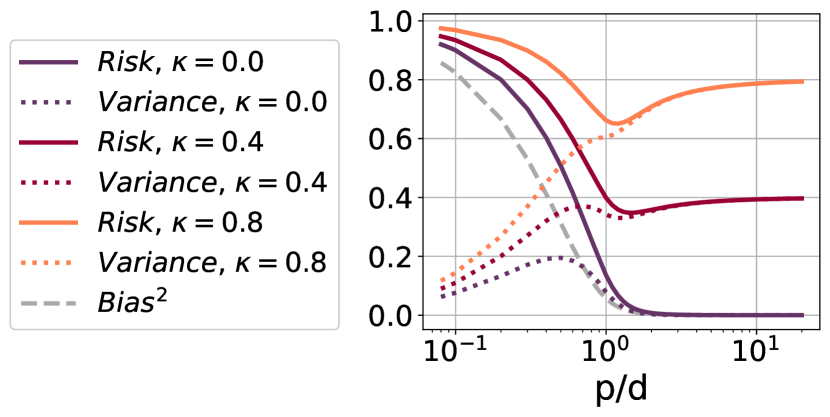
Figure 1: Decomposition of test loss. $\textbf{Risk}=\textbf{Bias}^{2}+\textbf{Variance}$. $\textbf{Bias}^{2}$ always monotonically decreases. Variance exhibits a transition from a unimodal shape to an increasing-decreasing-increasing pattern as noise increases, leading to the final ascent in test loss.

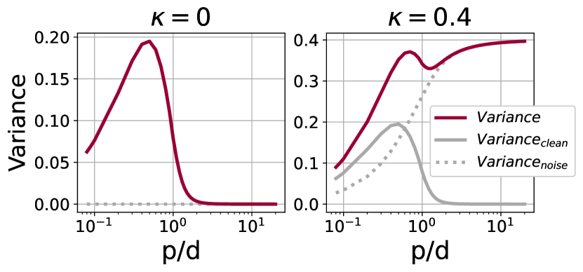
Figure 2: Decomposition of variance. $\textbf{Variance}=\textbf{Variance}_{\text{clean}}+\textbf{Variance}_{\text{noise}}$. $\textbf{Variance}_{\text{clean}}$ is always unimodal. $\textbf{Variance}_{\text{noise}}$ monotonically increases with width, and its scale grows with noise level, leading to the increasing-decreasing-increasing pattern of Variance at sufficient noise.

Suppose we have a training dataset $(\bm{X},\bm{y})$ where $\bm{X}=[\bm{x}_{1},\bm{x}_{2},\dots,\bm{x}_{n}]$ and $\bm{y}=[y_{1},y_{2},\dots,y_{n}]^{\top}$. Each input $\bm{x}_{i}\in\mathbb{R}^{d}$ is independently drawn from a Gaussian distribution $\mathcal{N}(0,\mathbf{I}_{d}/d)$. Each label $y_{i}\in\mathbb{R}$ is generated as $y_{i}=\bm{x}_{i}^{\top}\bm{\theta}+\epsilon_{i}$. Here, $\bm{\theta}\in\mathbb{R}^{d}$ has entries independently drawn from $\mathcal{N}(0,1)$, and $\epsilon_{i}\in\mathbb{R}$ is the label noise drawn from $\mathcal{N}(0,\sigma^{2})$ for each $\bm{x}_{i}$. We learn a two-layer linear network where the first layer $\bm{W}\in\mathbb{R}^{p\times d}$ has entries randomly drawn from $\mathcal{N}(0,1/d)$ and the second layer is given by

$$\hat{\bm{\beta}}=\operatorname*{arg\,min}_{\bm{\beta}\in\mathbb{R}^{p}}\|(\bm{W}\bm{X})^{\top}\bm{\beta}-\bm{y}\|^{2}+\lambda\|\bm{\beta}\|^{2}=(\bm{W}\bm{X}\bm{X}^{\top}\bm{W}^{\top}+\lambda\mathbf{I})^{-1}\bm{W}\bm{X}(\bm{X}^{\top}\bm{\theta}+\bm{\epsilon}),$$

where $\bm{\epsilon}=[\epsilon_{1},\epsilon_{2},\dots,\epsilon_{n}]^{\top}$. Given a test example with non-noisy label $(\bm{x},y)$ where $\bm{x}\sim\mathcal{N}(0,\mathbf{I}_{d}/d)$ and $y\!=\!\bm{x}^{\top}\bm{\theta}$, the prediction of the learned model is given by $f(\bm{x})\!=\!(\bm{W}\bm{x})^{\top}\hat{\bm{\beta}}$. The expected risk (test loss) can be written as

$$\textbf{Risk}= \mathbb{E}_{\bm{\theta}}\mathbb{E}_{\bm{x}}\mathbb{E}_{\bm{X},\bm{W},\bm{\epsilon}}(f(\bm{x})-y)^{2}=\underbrace{\mathbb{E}_{\bm{\theta}}\mathbb{E}_{\bm{x}}(\mathbb{E}_{\bm{X},\bm{W},\bm{\epsilon}}f(\bm{x})-y)^{2}}_{\textbf{Bias}^{2}}+\underbrace{\mathbb{E}_{\bm{\theta}}\mathbb{E}_{\bm{x}}\mathbb{V}_{\bm{X},\bm{W},\bm{\epsilon}}f(\bm{x})}_{\textbf{Variance}}$$ (1)

$$= \underbrace{\frac{1}{d}\|\mathbb{E}_{\bm{X},\bm{W}}\bm{B}-\mathbf{I}\|_{F}^{2}}_{\textbf{Bias}^{2}}+\underbrace{\frac{1}{d}\mathbb{E}_{\bm{X},\bm{W}}\|\bm{B}-\mathbb{E}_{\bm{X},\bm{W}}\bm{B}\|_{F}^{2}}_{\textbf{Variance}_{\text{clean}}}+\underbrace{\frac{\sigma^{2}}{d}\mathbb{E}_{\bm{X},\bm{W}}\|\bm{A}\|_{F}^{2}}_{\textbf{Variance}_{\text{noise}}},$$ (2)

where $\bm{A}\coloneqq\bm{W}^{\top}(\bm{W}\bm{X}\bm{X}^{\top}\bm{W}^{\top}+\lambda\boldsymbol{I})^{-1}\bm{W}\bm{X}$ and $\bm{B}\coloneqq\bm{A}\bm{X}^{\top}$ (see the derivation in Appendix A.1). Eq. 1 decomposes the risk into bias and variance, and Eq. (2) subsequently breaks down the variance into two terms. The second term, $\textbf{Variance}_{\text{noise}}$, captures the impact of label noise.

Our analysis is conducted under the high-dimensional asymptotic limit where $n$, $d$, and $p$ tend to infinity, while maintaining the ratios $\frac{n}{d}=\psi$, $\frac{p}{d}=\gamma$, and $\frac{\sigma^{2}}{(n/d)}=\kappa$ constant. To simplify the analysis further, we set $\psi=\infty$. This limit is consistent with the one used in Yang et al. (2020), which has been shown to capture important features of the double descent phenomenon. Our numerical experiments in Section 4.1 confirms that our conclusions hold in a broader range of settings outside of this regime. It is worth noting that the noise-to-sample size ratio $\kappa$ remains finite, despite the infinite value of $\psi$. We provide the explicit expression for $\textbf{Variance}_{\text{noise}}$ below.

Theorem 3.1.

For a 2-layer linear network with $p$ hidden neurons and a random first layer, consider learning the second layer by ridge regression with regularizer $\lambda$ on $n$ training examples with feature dimension $d$, and label noise with variance $\sigma$. Let $\lambda=\frac{n}{d}\lambda_{0}$ and $\sigma^{2}=\frac{n}{d}\kappa$ for some fixed $\lambda_{0}$ and $\kappa$. The asymptotic expression (where $n,d,p\rightarrow\infty$ with $\frac{n}{d}=\infty$ and $\frac{p}{d}=\gamma$) of $\textbf{Variance}_{\text{noise}}$ is given by

$$\frac{\kappa}{2}\left(\gamma+2\lambda_{0}+1-\frac{\gamma^{2}+(3\lambda_{0}-2)\gamma+2\lambda_{0}^{2}+3\lambda_{0}+1}{\sqrt{\gamma^{2}+(2\lambda_{0}-2)\gamma+\lambda_{0}^{2}+2\lambda_{0}+1}}\right)$$

We provide the derivation of $\textbf{Variance}_{\text{noise}}$ in Appendix A.3. Note that $\textbf{Bias}^{2}$ monotonically decreases and $\textbf{Variance}_{\text{clean}}$ is unimodal Yang et al. (2020) (see Appendix A.2 for expressions of $\textbf{Bias}^{2}$ and $\textbf{Variance}_{\text{clean}}$). By plotting the theoretical expressions, we make the following key observations.

The Noise-dependent Variance Shapes the Final Ascent. Figure 2 shows Variance by solid purple, $\textbf{Variance}_{\text{clean}}$ in solid gray, and $\textbf{Variance}_{\text{noise}}$ in dashed gray. We see that the shape of $\textbf{Variance}_{\text{clean}}$ is unimodal, while $\textbf{Variance}_{\text{noise}}$ monotonically increases with width. According to Theorem 3.1, we know that $\textbf{Variance}_{\text{noise}}$ scales with noise-to-sample size ratio ($\kappa$). Intuitively, variance measures the sensitivity to fluctuations in data and training. As the noise level increases, it has the potential to introduce greater inconsistency among the outputs of models, and this inconsistency grows as the model size increases. We see from the figure that $\kappa$ increases, $\textbf{Variance}_{\text{noise}}$ becomes more pronounced in the total variance, resulting in an increasing-decreasing-increasing trend. Therefore, the risk, which is the sum of Variance and the monotonically increasing $\textbf{Bias}^{2}$ (Figure 2), finds its minimum at an intermediate width when $\kappa$ is sufficiently large.

Regularization Exacerbates Final Ascent.

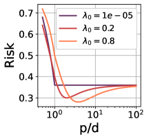
Figure 3: With stronger regularization, the optimal width increases and achieves lower loss, making the final ascent more pronounced.

Regularization is often used to improve robustness to noise, leading to the expectation that it would mitigate the impact of label noise and alleviate the final ascent phenomenon. However, Figure 3 shows that stronger $\ell_{2}$ regularization actually exacerbates the final ascent. We see that the final ascent is hardly visible with very small regularization, but becomes more pronounced as regularization increases. Specifically, larger regularization amplifies the advantage of intermediate widths, allowing them to achieve lower test loss. In Section 4.4, we show a similar observation for robust learning algorithms, which can be viewed as using very strong regularization.

Increasing Sample Size Alleviates Final Ascent. In our setting, although $\frac{n}{d}$ tends towards infinity, the impact of sample size is still evident through the constant noise-to-sample-size ratio $\kappa$. Importantly, Theorem 3.1 reveals that $\textbf{Variance}_{\text{noise}}$ scales with $\kappa$, rather than solely with the noise $\sigma^{2}$. Thus, increasing the sample size reduces the scaling of $\textbf{Variance}_{\text{noise}}$, thereby mitigating the final ascent phenomenon. This suggests that collecting more data is beneficial, even when the labels are noisy, as we will confirm empirically in Section 4.2.

In Section 4.1, we will conduct numerical experiments confirming that the final ascent is not limited to finite $\frac{n}{d}$. Indeed, it can occur in many other settings, even when $n<d$.

3.2 Beyond Width: Effect of Model Density

Next, we investigate the scenario where the model width is fixed, but the model density—fraction of weights that are trainable—is decreased by masking a predetermined set of parameters during the training process. There are several reasons why studying the effect of density is important: Firstly, changing density allows for a fine-grained control of capacity, unlike changing width which only results in $(\text{width}\times m)$ parameters, where $m$ is the number of parameters at width $1$. Secondly, changing density is less constrained by the model architecture, which is particularly relevant for complex architectures like InceptionResNet-v2 (which we use in our experiments in Section 4.3), where reducing width is difficult. Most importantly, as we show theoretically and empirically, density has a distinct effect on generalization compared to width, and finding the optimal width under smaller density can further improve generalization under label noise.

We consider the case where we randomly drop a set of trainable parameters instead of following certain criteria as in Jin et al. (2022). This isolates the effect of model size from any other factors.

The setting in Theorem 3.1, where the trainable layer has a scalar output, cannot differentiate between reducing density and reducing width. To address this, we consider a three-layer linear network in which the first layer yields random features, the second layer is randomly masked and trained, and the last layer is also random. The function represented by the network is formally defined as $f(\bm{x})=\left((\bm{V}\odot\bm{M})\bm{W}\bm{x}\right)^{\top}\bm{\mu}$. The first layer parameters $\bm{W}$ and input data $\bm{X}$ are the same as in Theorem 3.1. $\bm{V}\in\mathbb{R}^{q\times p}$ represents the second-layer parameters, and $\bm{M}\in\{0,1\}^{q\times p}$ is the mask applied to $\bm{V}$. The entries in $\bm{M}$ are independently drawn from a Bernoulli distribution with parameter $\alpha\in[0,1]$, where $\alpha$ represents the density. $\bm{\mu}\in\mathbb{R}^{q}$ represents the last-layer parameter, and its entries are independently drawn from $\mathcal{N}(0,1/q)$ (the variance is set to $1/q$ so that $q$ does not appear in the final expressions). We study other variants, such as setting it to $1/d$ and letting $q=p$ in Appendix A.6. We show that the risk and its decomposition in this setting can be derived by replacing $\lambda_{0}$ in Theorem 3.1 with $\lambda_{0}/\alpha$. See the proof in Appendix A.4.

Theorem 3.2.

For a 3-layer linear network with $p$ hidden neurons in the first layer and random first and last layers, consider learning the second layer by ridge regression with random masks drawn from $Bernoulli(\alpha)$. Let $\lambda$, $n$ and $\sigma$ be the ridge regression parameter, number of training examples and noise level, respectively. Let $\lambda=\frac{n}{d}\lambda_{0}$ and $\sigma^{2}=\frac{n}{d}\kappa$ for some fixed $\lambda_{0}$ and $\kappa$. The asymptotic expressions (where $n,d,p\rightarrow\infty$ with $\frac{n}{d}=\infty$ and $\frac{p}{d}=\gamma$) of Risk, $\textbf{Bias}^{2}$, $\textbf{Variance}_{\text{clean}}$ and $\textbf{Variance}_{\text{noise}}$ are given by their counterparts in the setting of Theorem 3.1 with $\lambda_{0}$ substituted with $\lambda_{0}/\alpha$.

(a) $\kappa=0$, Risk vs. $\alpha$

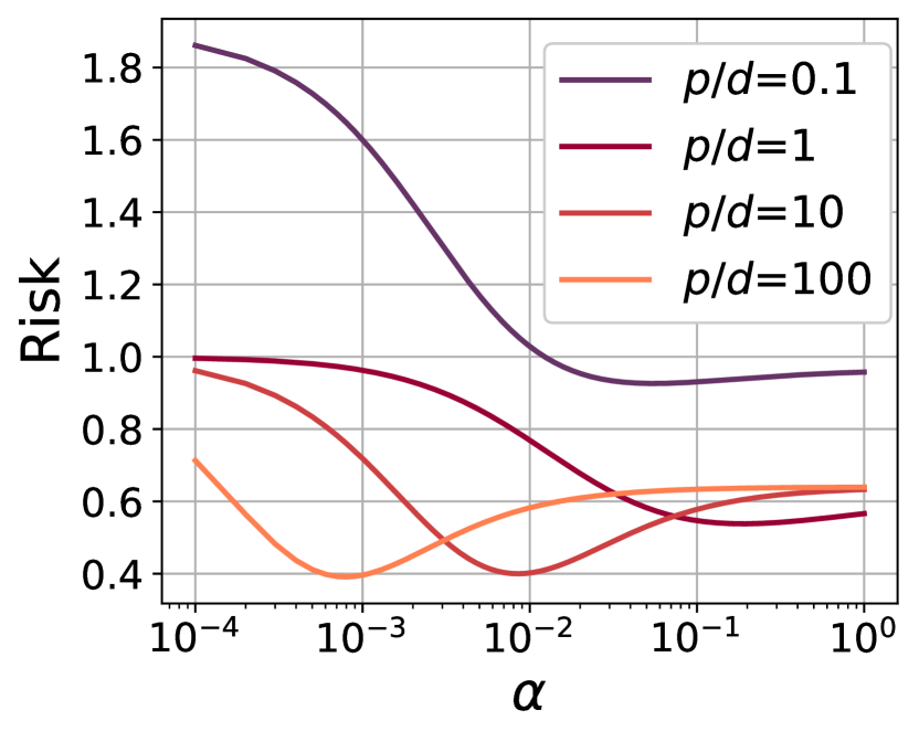
(b) $\kappa=0.64$, Risk vs. $\alpha$

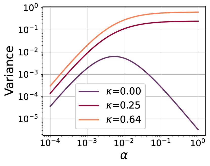
(c) $\frac{p}{d}=10$, Variance vs. $\alpha$

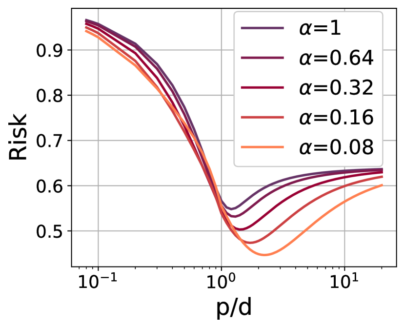
(d) $\kappa=0.64$, Risk vs. $p/d$

Figure 4: (a), (b): The risk curve changes from decreasing to U-shaped as the noise-to-sample-size ratio ($\kappa$) increases, for different values of width ($p$). (c) The total variance changes from unimodal to increasing as $\kappa$ increases. (d) Under lower density, the optimal width tends to be larger, and achieves lower test loss compared to the optimal width at higher density.

By plotting the theoretical expressions, we make the following key observations.

Reducing Density Can Improve Generalization Under Label Noise. In Figure 4, we set $\lambda_{0}$ to $0.05$ and plot the risk and variance based on Theorem 3.2. When there is no noise, we observe a decrease in risk as density ($\alpha$) increases (Figure 4(a)), accompanied by a unimodal behavior of the variance (Figure 4(c)). However, when the noise-to-sample size ratio ($\kappa$) is sufficiently large, the risk exhibits a U-shape (Figure 4(b)), while the variance monotonically increases (Figure 4(d)).

Better Generalization Can be Achieved at Larger Width with Lower Density. Theorem 3.2 demonstrates that reducing density is equivalent to a stronger $\ell_{2}$ regularization. Although in Section 4.3 we will empirically demonstrate that reducing density has effects beyond $\ell_{2}$ regularization for neural networks, it is already evident here that reducing density has a different effect than reducing width, even though both control the number of parameters. Furthermore, we observe from Figure 4(b) that the optimal density at a fixed width results in lower test loss as the width increases. Additionally, Figure 4(d) demonstrates that the optimal width for a given density increases as the density decreases, yielding lower test loss. This highlights the advantages of wider but sparser networks.

We note that our theory encompasses the empirical finding in Golubeva et al. (2020) that increasing width while keeping the number of parameters fixed improves generalization and this behavior can be altered by label noise similar to double descent (see Appendix A.7), although this is not the main focus of our paper.

4 Experiments on The Final Ascent Phenomenon

4.1 Final Ascent in Random Feature Ridge Regression with Different $\frac{n}{d}$ Ratios

In section 3.2, we theoretically showed that the final ascent can occur in the limit where $\frac{n}{d}\rightarrow\infty$, while $\frac{p}{d}$ remains constant. However, a natural question arises regarding whether the same conclusion holds when $\frac{n}{d}$ is finite. Characterizing the variance exactly is extremely troublesome when $\lambda>0$, as it involves finding solutions for a complicated fourth-degree equation when and taking derivatives, as shown by Adlam and Pennington (2020a). Hence, we conduct numerical experiments with finite values of $d$ and $n$ with varying $\frac{n}{d}$. Our results indicate that the final ascent can occur in many other settings, even when $n<d$. We plot the test loss (Figure 5) and total variance (Figure 17) against $p$. Legends show the values of $\sigma^{2}$, and titles show the values of $n/d$. We can clearly observe the final ascent when $\frac{n}{d}=$ $0.5,1,2,$ $4$.

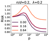
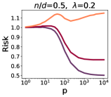
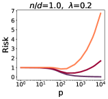
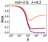
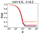
Figure 5: We plot the test loss in random feature ridge regression while fixing $d=100$ and $\lambda=0.2$, and varying $\sigma^{2}$. Legends show the values of $\sigma^{2}$, and titles show the values of $n/d$.

Table 1: Shape and scale of $\frac{\textbf{Variance}_{\text{noise}}}{\sigma^{2}}$ for different $n/d$ and $\sigma$. Scale is the value of $\frac{\textbf{Variance}_{\text{noise}}}{\sigma^{2}}$ at $p=10^{4}$.

	$n/d$	0.2	0.5	1	2	4
$\lambda$=0.01	Shape	$\nearrow\searrow$	$\nearrow\searrow$	$\nearrow$	$\nearrow$	$\nearrow$
	Scale	0.26	1.0	50.2	1.0	0.33
$\lambda$=0.2	Shape	$\nearrow\searrow$	$\nearrow$	$\nearrow$	$\nearrow$	$\nearrow$
	Scale	0.25	1.0	10.5	1.0	0.33

Effects of $n/d$ and $\lambda$ on the shape of $\textbf{Variance}_{\text{noise}}$.

Table 1 summarizes the shape and scale of $\frac{1}{\sigma^{2}}\textbf{Variance}_{\text{noise}}$ (i.e., $\frac{1}{d}\mathbbm{E}_{\bm{X},\bm{W}}\|\bm{A}\|_{F}^{2}$ according to Eq. 2) w.r.t. $p$ for different values of $\frac{n}{d}$ and $\lambda$ (plots are in Figures 18 and 19). Note that according to the decomposition in Eq. 2, whether the final ascent can possibly occur depends solely on if $\frac{1}{\sigma^{2}}\textbf{Variance}_{\text{noise}}$ increases in the end. We make the following observations: (1) Neither $n/d$ nor $\lambda$ alone can determine the shape of $\frac{1}{\sigma^{2}}\textbf{Variance}_{\text{noise}}$; (2) When both $\frac{n}{d}$ and $\lambda$ are small, $\frac{1}{\sigma^{2}}\textbf{Variance}_{\text{noise}}$ is unimodal, and the final ascent never occurs; (3) The effect of $n$ on the occurrence of the final ascent is non-monotonic: when $\frac{n}{d}\leq 1$, increasing $n$ turns $\frac{1}{\sigma^{2}}\textbf{Variance}_{\text{noise}}$ from unimodal to monotonically increasing, leading to the final ascent. However, when $n/d>1$, increasing $n$ scales down $\frac{1}{\sigma^{2}}\textbf{Variance}_{\text{noise}}$ while preserving its monotonically increasing shape, resulting in the final ascent being less pronounced. This second half of the observation is captured by Theorem 3.1 showing that $\textbf{Variance}_{\text{noise}}$ scales with $\frac{\sigma^{2}}{n/d}$. These observations reveal a complex behavior of the variance and highlight the need for future theoretical research to fully explain it.

4.2 Final Ascent in Neural Networks: Effect of Width

Next, we empirically demonstrate the occurrence of the final ascent in neural networks trained with label noise across various settings. Although our theoretical results (Section 3.1) are based on regression, our empirical findings confirm that the theoretical insights hold for classification with neural networks.

We conduct a comprehensive set of experiments to thoroughly investigate the factors influencing the final ascent. Our study involve three datasets: MNIST LeCun (1998), CIFAR-10, and CIFAR-100 (Krizhevsky et al., 2009). We train two-layer ReLu networks on MNIST, and train ResNet34He et al. (2016) on CIFAR-10/100. We examine two types of loss functions: mean squared error (MSE) loss and cross-entropy (CE) loss. MSE loss enables more accurate measurement of the bias and variance in test loss Yang et al. (2020) (see details Appendix C.2 ), allowing us to empirically observe the transition in the shape of variance shown in Theorem 3.1. We consider two types of noise: symmetric noise generated through random label flipping and asymmetric noise generated in a class-dependent manner (see Appendix C.1). Asymmetric noise better resembles real-world noise distributions Patrini et al. (2017). Further experimental details can be found in Appendix C. We make the following analysis of our experimental results.

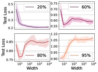
(a)

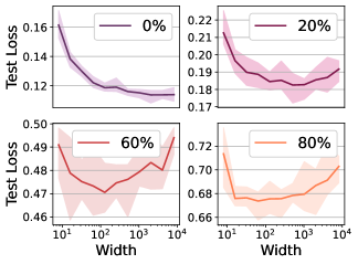
(b)

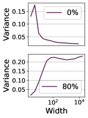
(c)

Figure 6: Test loss and total variance on MNIST using MSE loss with (a) $\lambda=0$ and (b) $\lambda=0.001$ ($l_{2}$ regularization). We split the original dataset into 20 subsets to measure bias and variance (see details Appendix C.2). Final ascent occurs when the noise level reaches a certain threshold. Stronger regularization exacerbates the final ascent phenomenon and reduces the required noise level. (c) As the noise level increases, the variance transitions from a unimodal shape to an increasing-decreasing-increasing pattern.

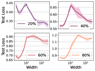
(a)

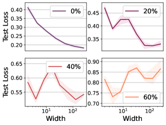
(b)

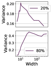
(c)

Figure 7: Test loss and total variance on CIFAR-10 using MSE loss with (a) $\lambda=0.0005$ and (b) $\lambda=0.001$. We split the original dataset into 5 subsets to measure bias and variance (see details Appendix C.2). The observed patterns are consistent with Figure 6, confirming that stronger regularization exacerbates the final ascent and that increasing noise causes the transition in the variance shape.

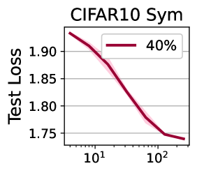
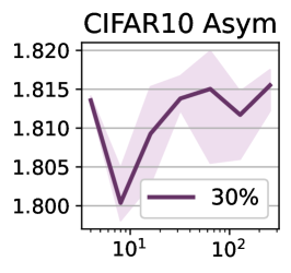
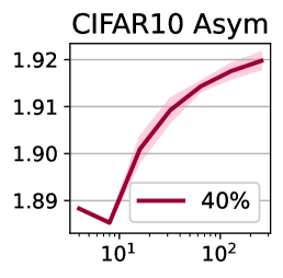
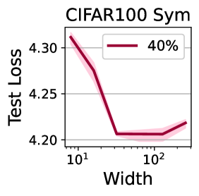
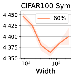
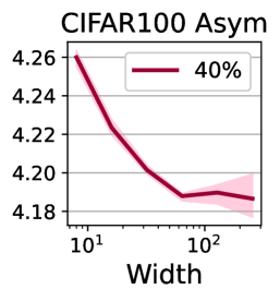
Figure 8: Results for models trained with symmetric and asymmetric noise on full CIFAR-10/100 using CE loss. $\lambda=0.0005$.

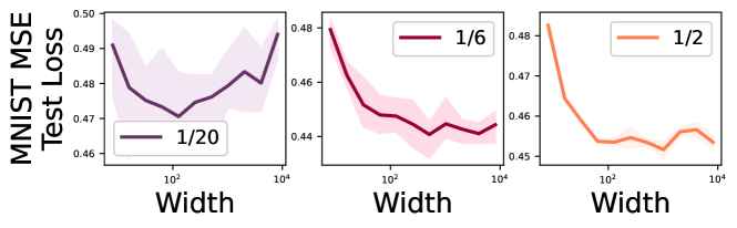
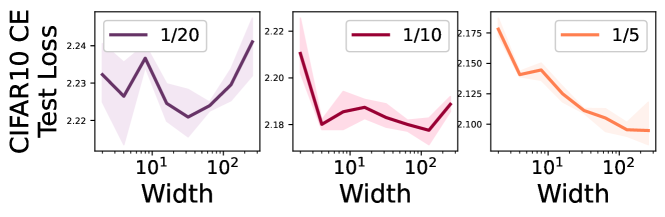
Figure 9: Test loss obtained with different sample sizes for MNIST using MSE loss (top) and CIFAR-10 using CE loss (bottom). We use $\lambda$=0.001 and 60% noise for both. Legends indicate the fraction of data used for training.

The Final Ascent Occurs in Various Settings. Figures 6 to 9 demonstrate the presence of final ascent across different model architectures, loss functions, and noise types. For instance, in Figures 6 and 7, as the noise level increases, we observe a transition in the loss curve from double descent or monotonically decreasing to a curve with final ascent. The corresponding test accuracy plots can be found in Appendix D.1.

Transition of the Shape of Variance as Label Noise Increases. As discussed in Section 3.1, the final ascent in the test loss is attributed to the increasing-decreasing-increasing pattern of the variance. The results presented in Figures LABEL:subfig:mnist_var and LABEL:subfig:cifar10_var confirm that this holds true for neural networks. The shape of the variance curve turns from unimodal to increasing-decreasing-increasing as the level of noise increases, matching our theoretical results.

Stronger $\ell_{2}$ Regularization Exacerbates Final Ascent. Our theoretical analysis in Section 3.1 demonstrates that stronger regularization exacerbates final ascent. This finding is further corroborated by our experimental results, as evidenced by comparing Figures LABEL:subfig:mnist_risk and LABEL:subfig:mnist_risk_Wd, as well as Figures LABEL:subfig:cifar10_risk and LABEL:subfig:cifar10_risk_wd. For example, on CIFAR-10 with 20% noise, the test loss curve exhibits the well-known double descent when $\lambda=0.0005$ (the parameter of $l_{2}$ regularization), while it demonstrates the final ascent phenomenon when $\lambda=0.001$. Note that using regularization often yields a better result.

Asymmetric Noise May Exacerbate Final Ascent. Figure 9 shows that asymmetric noise significantly exacerbates the final ascent on CIFAR-10. Under 40% noise, the final ascent is absent for symmetric noise but present for asymmetric noise. However, this trend is not obvious on CIFAR-100, possibly because asymmetric noise is generated differently on these two datasets (see Appendix C.1) with the noise on CIFAR-100 being less skewed.

Larger Sample Size Alleviates Final Ascent. As shown in Theorem 3.1, the scale of $\textbf{Variance}_{\text{noise}}$ is determined by the noise-to-sample-size ratio rather than the noise level itself, implying that increasing the sample size can counteract the impact of noise and alleviate the occurrence of final ascent. This is further confirmed by our experimentals. Figure 9, shows the test loss curves obtained with varying sample sizes on MNIST (using MSE loss) and CIFAR-10 dataset (using cross-entropy loss). The final ascent occurs when only $1/20$ of the original data is used, but not when the dataset size is increased to $1/2$ for MNIST and $1/5$ for CIFAR-10.

Required Noise Level for Final Ascent. Based on the preceding discussions, it becomes evident that the required noise level depends on several factors, including the degree of regularization, the sample size, and the nature of the noise distribution. In general, a lower noise level is required with strong regularization, smaller sample sizes, and strong noise types. Notably, the required noise level can be as low as 20% (Figures 6, 7). On CIFAR-10, even with full data and the commonly used small regularization ($5$e^-4), final ascent occurs under only 30% asymmetric noise (Figure 9). In practice, where the noise typically resembles asymptotic noise and strong regularization is applied in the presence of noise, final ascent is highly likely to occur under low noise levels.

4.3 Final Ascent in Neural Networks: Effect of Density

Next, we study the effect of density by conducting experiments on three datasets: MNIST, CIFAR-10, and Red Stanford Cars Jiang et al. (2020) containing real-world label noise, as detailed in Appendix C.1. We train an InceptionResNet-v2 model on Red Stanford Cars . Since the InceptionResNet-v2 architecture is intricate, there is no straightforward way to vary its width, and demands reducing density. Other details are in Appendix C. We make the following analysis of the experimental results.

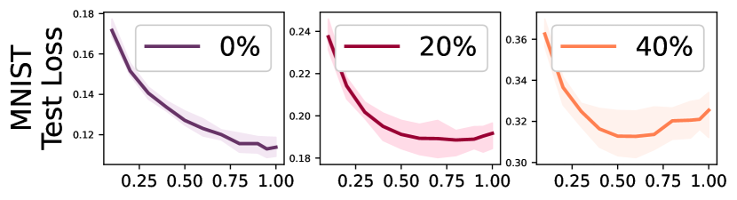
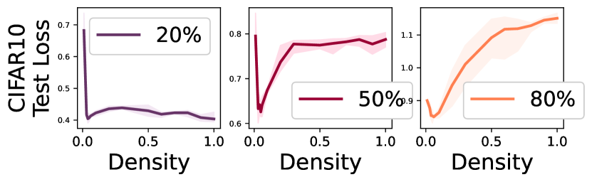
(a) MNIST and CIFAR-10

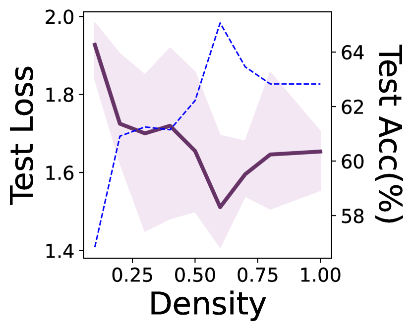
(b) Cars, 30% noise

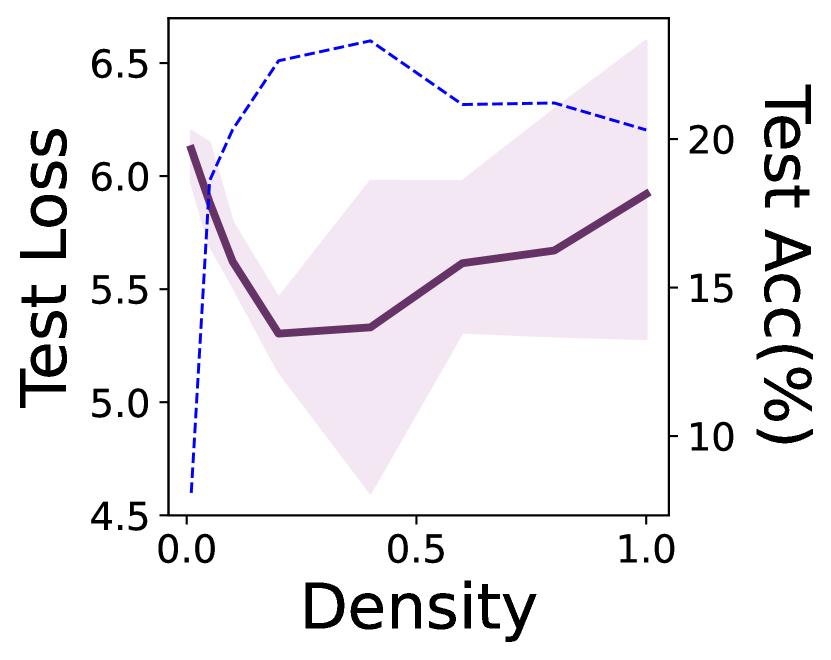
(c) Cars, 70% noise

Figure 10: Test performance models with varied densities on (a) MNIST and CIFAR-10 and (b) Red Stanford Car. In (a) legends indicate noise ratios. We observe that the test loss curve changes from a decreasing trend to a U-shape as noise increases. In (b) the purple solid line shows test loss and the blue dashed line shows accuracy.

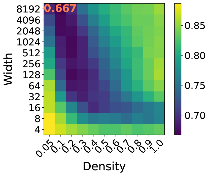
(a) Test Loss (MNIST)

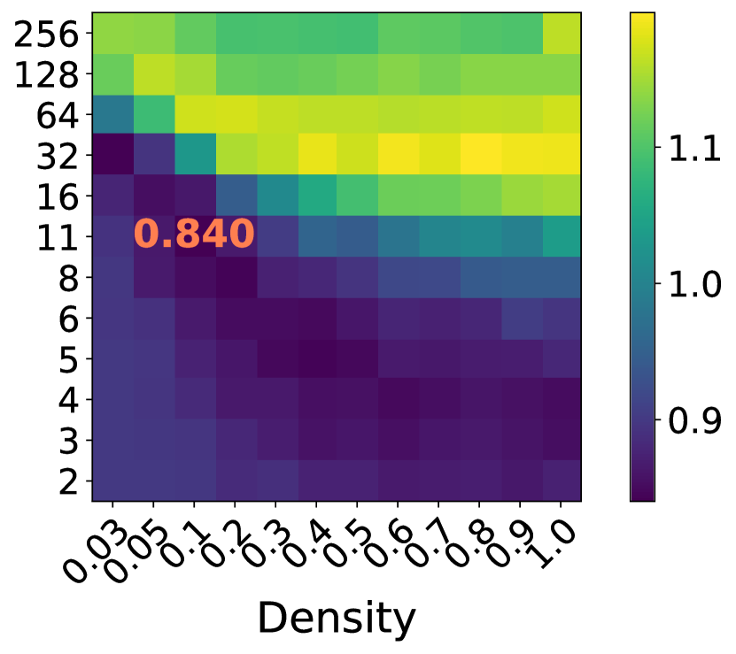
(b) Test Loss (CIFAR-10)

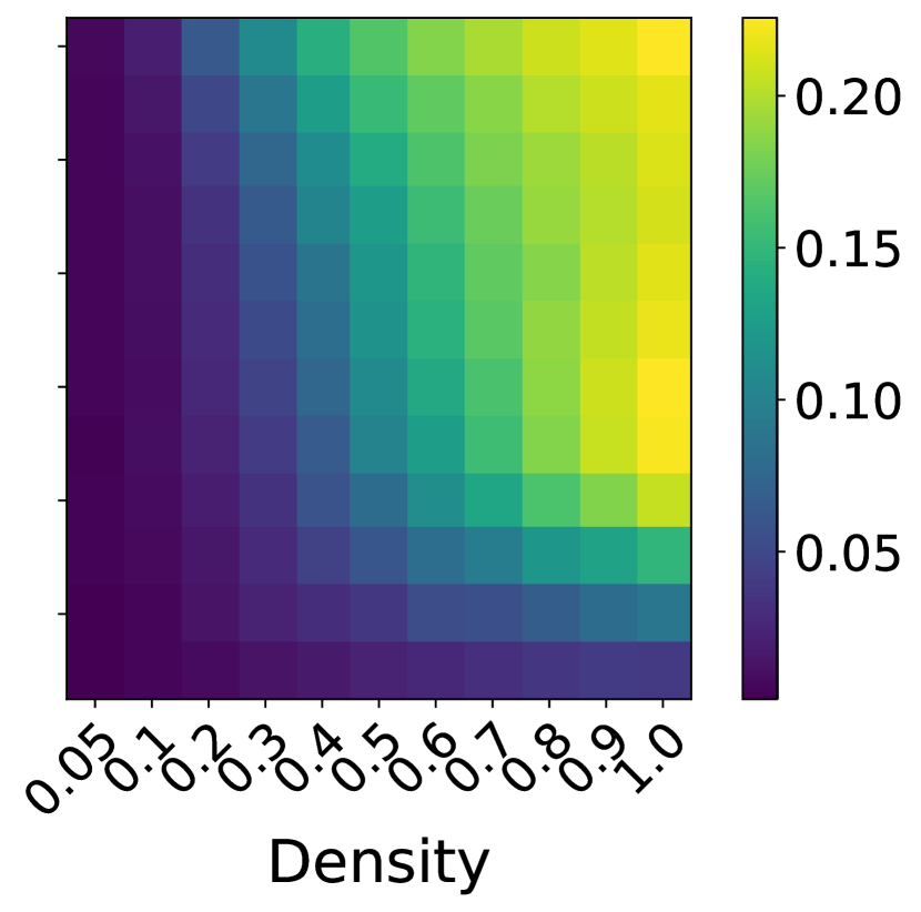
(c) Variance (MNIST)

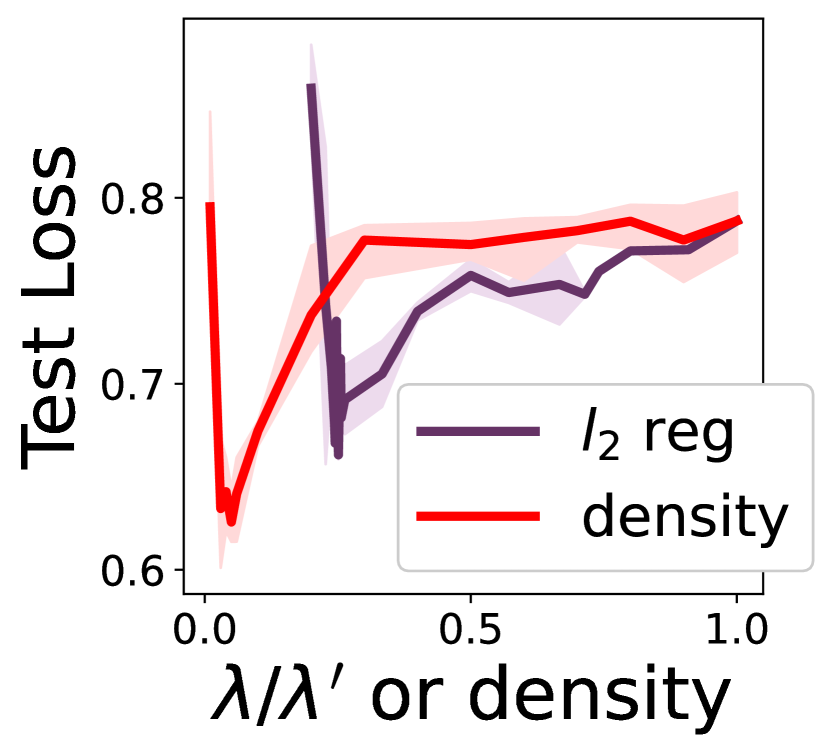
(d) Density vs. $l_{2}$ reg

Figure 11: Test loss (a) (b) and variance (c) of models at varied widths and densities. In (d) we compare the effects of varying density and varying $l_{2}$ regularization. When varying $\lambda$, density is fixed to 1. When varying density, $\lambda$ is fixed to $\lambda^{\prime}=0.0005$. The x-axis represents the inverse of the scale-up of $\lambda$, i.e., $\lambda/\lambda^{\prime}$, for the regularization curve (purple), and density for the density curve (red).

Reducing Density Improves Generalization. Figure 10 shows that when the label noise is small (e.g., 0% on MNIST, 20% on CIFAR-10), test loss improves as density increases. In contrast, when the label noise is sufficiently large (e.g., 40% on CIFAR-10, 50% on MNIST, 30%/70% on Red Stanford Car), the lowest test loss is achieved at an intermediate density.

Joint Effect of Density and Width. Figures 11(c) shows an increasing trend in variance towards the top-right corner. Figures 11(a) and 11(b) show that models with low loss (darkest blue) are distributed along the diagonal and the lowest loss (annotated in red) is achieved with models with very small density. This confirms our theoretical results in Section 3.2 that models of optimal width under smaller density exhibit better generalization, and highlights the importance of considering both width and density in improving the performance. Test accuracy and bias are shown in Appendix D.2.

Reducing Density has an Effect Beyond $\ell_{2}$ Regularization for Neural Networks. Theorem 3.2 shows that reducing density is equivalent to increasing the $\ell_{2}$ regularization by the inverse factor for random feature ridge regression. However, Figure 11(d) (test accuracy is in Appendix D.2) shows that reducing density of neural networks has an effect beyond $\ell_{2}$ regularization. Although both loss curves exhibit a U shape, bottom of the U shape for density is lower than that of varying $\ell_{2}$ regularization. In other words, adjusting density can achieve a lower loss than adjusting $\ell_{2}$ regularization.

4.4 Final Ascent in Neural Networks: Robust Learning Algorithms

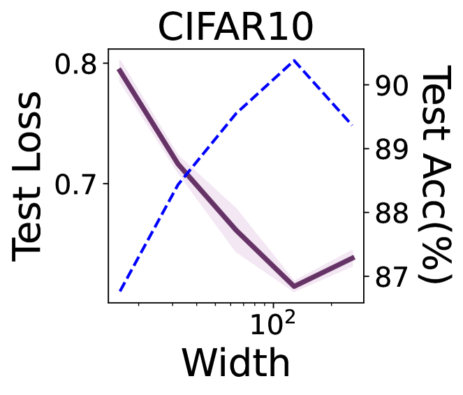
(a) ELR, Sym, 40%

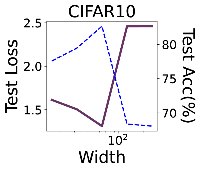
(b) ELR, Asym, 40%

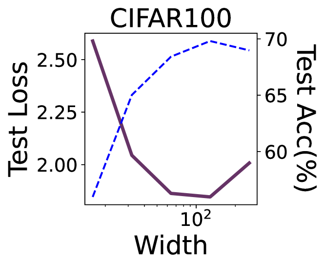
(c) ELR, Sym, 40%

(d) DivideMix, Sym, 60%

Figure 12: Test loss (solid line) and accuracy (dashed line) of models trained with ELR and DivideMix on CIFAR-10/100. Comparing (a) with Figure 9, we see that ELR even makes the final ascent more pronounced.

We study the effect of robust learning methods, which are typically employed in the presence of label noise, on the final ascent phenomenon. We consider two state-of-the-art algorithms, ELR (Liu et al., 2020) and DivideMix (Li et al., 2020) on CIFAR-10 and CIFAR-100 (details in Appendix C.4). Interestingly, we see that the final ascent can still be observed (Figures 12 and 28), and in some cases is even exacerbated. For example, without ELR, the final ascent is not observed on CIFAR-10 under 60% symmetric noise with only $1/5$ of the data (Figure 9). In contrast, when ELR is applied, the final ascent occurs under only 40% symmetric noise on the full data. Additional experiments are presented in Appendix D.3. The final ascent regarding model density is also observed in Figures 29 to 31.

Connection to $\ell_{2}$ Regularization. The presence of the final ascent when using robust algorithms aligns with our previous theoretical and empirical findings that stronger $\ell_{2}$ regularization exacerbates this phenomenon. As robust algorithms can be viewed as a form of stronger regularization compared to $\ell_{2}$, it is not surprising that they amplify the final ascent rather than mitigating it.

5 Conclusion and Discussion

In this work, we present the final ascent, an intriguing phenomenon, with respect to both model width and density. Through comprehensive theoretical and empirical studies, we reveal important findings including the transition in variance shape, the interplay between width and density, as well as the roles of sample size, regularization, and robust methods.

While our theory captures important features of the variance curve, the experiments in Section 4.1 reveal a more complex behavior of the variance, which depends on multiple factors. Developing a more comprehensive theory to fully explain the observed patterns could be an important future direction.

The findings on sample size and regularization/robust methods provide practical guidance. When addressing label noise with large regularization or robust methods, it is advisable to have a sufficiently large sample size in order to confidently employ larger models. Otherwise, caution should be exercised in selecting the model size. Future research aimed at developing precise criteria for determining whether a given setting falls within the ‘larger models can be used freely’ regime would be valuable.

Appendix A Theoretical Results

Notations: We use bold-faced letter for matrix and vectors. The training dataset is denoted by $(\bm{X},\bm{y})$ where $\bm{X}=[\bm{x}_{1},\bm{x}_{2},\dots,\bm{x}_{n}]$ and $\bm{y}=[y_{1},y_{2},\dots,y_{n}]^{\top}$. Each input vector $\bm{x}_{i}\in\mathbb{R}^{d}$ is independently drawn from a Gaussian distribution $\mathcal{N}(0,\mathbf{I}_{d}/d)$. Each label $y_{i}\in\mathbb{R}$ is generated by $y_{i}=\bm{x}_{i}^{\top}\bm{\theta}+\epsilon_{i}$. We assume $\bm{\theta}\in\mathbb{R}^{d}$ has its entries independently drawn from $N(0,1)$. $\epsilon_{i}\in\mathbb{R}$ is the label noise drawn from $N(0,\sigma^{2})$ for each $\bm{x}_{i}$. We assume each test example $(\bm{x},y)$ is clean, i.e., $y=\bm{x}^{\top}\bm{\theta}$.

A.1 Bias-Variance Decomposition of the MSE Loss in Section 3.1

Here we show the derivation of Equation 1.

$$\textbf{Bias}^{2}= \mathbb{E}_{\bm{\theta}}\mathbb{E}_{\bm{x}}(\mathbb{E}_{\bm{X},\bm{W},\bm{\epsilon}}f(\bm{x})-y)^{2}$$

$$= \mathbb{E}_{\bm{\theta}}\mathbb{E}_{\bm{x}}(\mathbb{E}_{\bm{X},\bm{W},\bm{\epsilon}}((\bm{W}\bm{x})^{\top}\hat{\bm{\beta}})-y)^{2}$$

$$= \mathbb{E}_{\bm{\theta}}\mathbb{E}_{\bm{x}}[\bm{x}^{\top}(\mathbb{E}_{\bm{X},\bm{W},\bm{\epsilon}}(\bm{B}\bm{\theta}+\bm{A}\bm{\epsilon})-\bm{\theta})]^{2}$$

$$= \mathbb{E}_{\bm{\theta}}\mathbb{E}_{\bm{x}}\operatorname{Tr}[(\mathbb{E}_{\bm{X},\bm{W},\bm{\epsilon}}(\bm{B}\bm{\theta})-\bm{\theta})^{\top}\bm{x}\bm{x}^{\top}(\mathbb{E}_{\bm{X},\bm{W},\bm{\epsilon}}(\bm{B}\bm{\theta})-\bm{\theta})]$$

$$= \mathbb{E}_{\bm{\theta}}\operatorname{Tr}[(\mathbb{E}_{\bm{X},\bm{W},\bm{\epsilon}}(\bm{B}\bm{\theta})-\bm{\theta})^{\top}\mathbb{E}_{\bm{x}}(\bm{x}\bm{x}^{\top})(\mathbb{E}_{\bm{X},\bm{W},\bm{\epsilon}}(\bm{B}\bm{\theta})-\bm{\theta})]$$

$$= \frac{1}{d}\mathbb{E}_{\bm{\theta}}\|\mathbb{E}_{\bm{X},\bm{W},\bm{\epsilon}}(\bm{B}\bm{\theta})-\bm{\theta}\|_{F}^{2}$$

$$= \frac{1}{d}\mathbb{E}_{\bm{\theta}}\operatorname{Tr}[(\mathbb{E}_{\bm{X},\bm{W}}\bm{B}-\mathbf{I})\bm{\theta}\bm{\theta}^{\top}(\mathbb{E}_{\bm{X},\bm{W}}\bm{B}-\mathbf{I})]$$

$$= \frac{1}{d}\operatorname{Tr}[(\mathbb{E}_{\bm{X},\bm{W}}\bm{B}-\mathbf{I})\mathbb{E}_{\bm{\theta}}(\bm{\theta}\bm{\theta}^{\top})(\mathbb{E}_{\bm{X},\bm{W}}\bm{B}-\mathbf{I})]$$

$$= \frac{1}{d}\|\mathbb{E}_{\bm{X},\bm{W}}\bm{B}-\mathbf{I}\|_{F}^{2}$$

$$\textbf{Variance}= \mathbb{E}_{\bm{\theta}}\mathbb{E}_{\bm{x}}\mathbb{V}_{\bm{X},\bm{W},\bm{\epsilon}}f(\bm{x})$$

$$= \mathbb{E}_{\bm{\theta}}\mathbb{E}_{\bm{x}}\mathbb{E}_{\bm{X},\bm{W},\bm{\epsilon}}[\bm{x}^{\top}(\bm{B}\bm{\theta}+\bm{A}\bm{\epsilon})-\mathbb{E}_{\bm{X},\bm{W},\bm{\epsilon}}\bm{x}^{\top}(\bm{B}\bm{\theta}+\bm{A}\bm{\epsilon})]^{2}$$

$$= \frac{1}{d}\mathbb{E}_{\bm{\theta}}\mathbb{E}_{\bm{X},\bm{W},\bm{\epsilon}}\|(\bm{B}\bm{\theta}+\bm{A}\bm{\epsilon})-\mathbb{E}_{\bm{X},\bm{W}}\bm{B}\bm{\theta}\|_{F}^{2}$$

$$= \frac{1}{d}\mathbb{E}_{\bm{\theta}}\mathbb{E}_{\bm{X},\bm{W},\bm{\epsilon}}\|(\bm{B}-\mathbb{E}_{\bm{X},\bm{W}}\bm{B})\bm{\theta}+\bm{A}\bm{\epsilon}\|_{F}^{2}$$

$$= \frac{1}{d}\mathbb{E}_{\bm{\theta}}\mathbb{E}_{\bm{X},\bm{W}}\|(\bm{B}-\mathbb{E}_{\bm{X},\bm{W}}\bm{B})\bm{\theta}\|_{F}^{2}+\frac{1}{d}\mathbb{E}_{\bm{X},\bm{W},\bm{\epsilon}}\|\bm{A}\bm{\epsilon}\|_{F}^{2}$$

$$= \underbrace{\frac{1}{d}\mathbb{E}_{\bm{X},\bm{W}}\|\bm{B}-\mathbb{E}_{\bm{X},\bm{W}}\bm{B}\|_{F}^{2}}_{\textbf{Variance}_{\text{clean}}}+\underbrace{\frac{\sigma^{2}}{d}\mathbb{E}_{\bm{X},\bm{W}}\|\bm{A}\|_{F}^{2}}_{\textbf{Variance}_{\text{noise}}}$$

A.2 Expressions of Bias and $\textbf{Variance}_{\text{clean}}$

Yang et al. [2020] analyzed the bias-variance decomposition without considering label noise. Hence the variance in their analysis corresponds to $\textbf{Variance}_{\text{clean}}$ in ours. We show their expressions of $\textbf{Bias}^{2}$ and $\textbf{Variance}_{\text{clean}}$ below, based on which we plot the dashed gray line in Figure 2 and the solid gray line in Figure 2.

$$\textbf{Bias}^{2}=\frac{1}{4}\Phi_{3}(\lambda_{0},\gamma)^{2}$$

$$\textbf{Variance}_{\text{clean}}=\begin{cases}\frac{\Phi_{1}(\lambda_{0},\gamma)}{2\Phi_{2}(\lambda_{0},\gamma)}-\frac{(1-\gamma)(1-2\gamma)}{2\gamma}-\frac{1}{4}\Phi_{3}(\lambda_{0},\gamma)^{2},\quad\gamma\leq 1,\\ \frac{\Phi_{1}(\lambda_{0},1/\gamma)}{2\Phi_{2}(\lambda_{0},1/\gamma)}-\frac{\gamma-1}{2}-\frac{1}{4}\Phi_{3}(\lambda_{0},\gamma)^{2},\quad\gamma>1,\end{cases}$$

where

$$\Phi_{1}(\lambda_{0},\gamma)= \lambda_{0}(\gamma+1)+(\gamma-1)^{2},$$

$$\Phi_{2}(\lambda_{0},\gamma)= \sqrt{(\lambda_{0}+1)^{2}+2(\lambda_{0}-1)\gamma+\gamma^{2}},$$

$$\Phi_{3}(\lambda_{0},\gamma)= \Phi_{2}(\lambda_{0},\gamma)-\lambda_{0}-\gamma+1.$$

A.3 Proof of Theorem 3.1

Lemma A.1.

Define $\tilde{\bm{B}}=\bm{W}^{\top}(\bm{W}\bm{W}^{\top}+\lambda_{0}\boldsymbol{I})^{-1}\bm{W}$. $\|\tilde{\bm{B}}\tilde{\bm{B}}^{\top}-\frac{n}{d}\bm{A}\bm{A}^{\top}\|_{2}=0$ almost surely, i.e., $\mathbb{P}(\|\tilde{\bm{B}}\tilde{\bm{B}}^{\top}-\frac{n}{d}\bm{A}\bm{A}^{\top}\|_{2}\leq\epsilon)\geq 1-\delta$ where $\epsilon$ and $\delta$ both tend to $0$ under the asymptotics $n\rightarrow\infty$, $d\rightarrow\infty$ and $n/d\rightarrow\infty$.

Proof.

Define

$$\bm{\Delta}\coloneqq \frac{d}{n}\bm{X}\bm{X}^{\top}-I,$$

$$\bm{\Psi}\coloneqq (\bm{W}\bm{W}^{\top}+\lambda_{0}I)^{-1}$$

$$\bm{\Gamma}\coloneqq (\frac{d}{n}\bm{W}\bm{X}\bm{X}^{\top}\bm{W}^{\top}+\lambda_{0}I)^{-1}$$

$$\bm{\Omega}\coloneqq \bm{\Gamma}-\bm{\Psi}.$$

Then we have

$$\tilde{\bm{B}}\tilde{\bm{B}}^{\top}-\frac{n}{d}\bm{A}\bm{A}^{\top}=~{} \bm{\Omega}\bm{W}\bm{\Delta}\bm{W}^{\top}\bm{\Omega}+\bm{\Psi}\bm{W}\bm{\Delta}\bm{W}^{\top}\bm{\Psi}+\bm{\Omega}\bm{W}\bm{\Delta}\bm{W}^{\top}\bm{\Psi}+\bm{\Psi}\bm{W}\bm{\Delta}\bm{W}^{\top}\bm{\Omega}$$

$$~{}~{}~{}~{}~{}~{}~{}~{}~{}~{}~{}~{}~{}~{}+~{}\bm{\Omega}\bm{W}\bm{W}^{\top}\bm{\Omega}+\bm{\Omega}\bm{W}\bm{W}^{\top}\bm{\Psi}+\bm{\Psi}\bm{W}\bm{W}^{\top}\bm{\Omega}.$$

By triangle inequality and the sub-multiplicative property of spectral norm we have

$$\|\tilde{\bm{B}}\tilde{\bm{B}}^{\top}-\frac{n}{d}\bm{A}\bm{A}^{\top}\|_{2}\leq~{} \|\bm{W}\|_{2}^{2}\|\bm{\Omega}\|_{2}^{2}\|\bm{\Delta}\|_{2}+\|\bm{W}\|_{2}^{2}\|\bm{\Psi}\|_{2}^{2}\|\bm{\Delta}\|_{2}+2\|\bm{W}\|_{2}^{2}\|\bm{\Psi}\|_{2}\|\bm{\Omega}\|_{2}\|\bm{\Delta}\|_{2}$$

$$+~{}\|\bm{W}\|_{2}^{2}\|\bm{\Omega}\|_{2}^{2}+2\|\bm{W}\|_{2}^{2}\|\bm{\Psi}\|_{2}\|\bm{\Omega}\|_{2}$$

It remains to show that with the asymptotic assumption $n/d\rightarrow\infty$, $\|\bm{\Omega}\|_{2}=0$ and $\|\bm{\Delta}\|_{2}=0$ almost surely, and $\|\bm{W}\|_{2}$ and $\|\bm{\Psi}\|$ can be bounded from above Yang et al. [2020]:

$$\mathbb{P}(\|\bm{\Delta}\|_{2}\leq 4\sqrt{\frac{d}{n}}+4\frac{d}{n})\geq 1-e^{-d/2}$$

$$\|\bm{\Omega}\|_{2}\leq\|\bm{\Psi}\|_{2}^{2}\|\bm{W}\|_{2}^{2}\|\bm{\Delta}\|_{2}+O(\|\bm{\Delta}\|_{2})$$

$$\|\bm{W}\|_{2}\overset{a.s.}{=}1+\sqrt{\eta}<\infty$$

$$\|\bm{\Psi}\|_{2}\leq\frac{1}{\lambda_{0}}<\infty.$$

Therefore we have $\|\tilde{\bm{B}}\tilde{\bm{B}}^{\top}-\frac{n}{d}\bm{A}\bm{A}^{\top}\|_{2}=0$ almost surely. ∎

Corollary A.2.

$\frac{\sigma^{2}}{d}\|\bm{A}\|^{2}_{F}=\frac{\kappa}{d}\|\tilde{\bm{B}}\|^{2}_{F}$ almost surely.

Proof.

By lemma A.1 we have

$$|\operatorname{Tr}(\frac{1}{n}\tilde{\bm{B}}\tilde{\bm{B}}^{\top}-\frac{1}{d}\bm{A}\bm{A}^{\top})|= ~{}\frac{1}{n}\operatorname{Tr}(\tilde{\bm{B}}\tilde{\bm{B}}^{\top}-\frac{n}{d}\bm{A}\bm{A}^{\top})$$

$$\leq ~{}\frac{d}{n}\|\tilde{\bm{B}}\tilde{\bm{B}}^{\top}-\frac{n}{d}\bm{A}\bm{A}^{\top}\|_{2}$$

$$= ~{}0,$$

which yields $\frac{1}{d}\|\bm{A}\|^{2}_{F}=\frac{1}{n}\|\tilde{\bm{B}}\|^{2}_{F}$ and thus $\frac{\sigma^{2}}{d}\|\bm{A}\|^{2}_{F}=\frac{\kappa}{d}\|\tilde{\bm{B}}\|^{2}_{F}$. ∎

Now it only remains to compute $\frac{1}{d}\|\tilde{\bm{B}}\|^{2}_{F}$. By Sherman–Morrison formula,

$$\tilde{\bm{B}}=I-(I+\frac{\alpha}{\eta}\bm{Q})^{-1},$$

where $\alpha=\lambda_{0}^{-1}$, $\bm{Q}=(d/p)\bm{W}^{\top}\bm{W}$ and $\eta=d/p=1/\gamma$. Let $F^{\bm{Q}}$ be the empirical spectral distribution of $\bm{Q}$, i.e.,

$$F^{\bm{Q}}(x)=\frac{1}{d}\#\{j\leq d:\lambda_{j}\leq x\},$$

where $\#S$ denotes the cardinality of the set $S$ and $\lambda_{j}$ denotes the $j$-th eigenvalue of $\bm{Q}$. Then

$$\frac{\|\tilde{\bm{B}}\|^{2}}{d}=\int_{\mathbb{R}^{+}}\frac{(\frac{\alpha}{\eta}x)^{2}}{(1+\frac{\alpha}{\eta}x)^{2}}dF^{\bm{Q}}(x).$$

By Marchenko-Pastur Law Bai and Silverstein [2010],

$$\frac{\|\tilde{\bm{B}}\|^{2}}{d}= \frac{1}{2\pi}\int_{\eta_{-}}^{\eta_{+}}\frac{\sqrt{(\eta_{+}-x)(x-\eta_{-})}(\frac{\alpha}{\eta}x)^{2}}{\eta x(1+\frac{\alpha}{\eta}x)^{2}}dx$$

$$= ~{}\frac{1}{2\alpha}\left(\frac{-\alpha^{2}/\eta^{2}-(3\alpha-2\alpha^{2})/\eta-\alpha^{2}-3\alpha-2}{\sqrt{\alpha^{2}/\eta^{2}+(2\alpha-2\alpha^{2})/\eta+\alpha^{2}+2\alpha+1}}+\alpha/\eta+\alpha+2\right).$$ (3)

Combining equation 3 and corollary A.2 and substituting $\alpha=\lambda_{0}^{-1},\eta=\gamma^{-1}$ into the result completes the proof.

A.4 Proof of Theorem 3.2

Define the following shorthand

$$\bm{F}\coloneqq \bm{W}\bm{X}$$

$$\bm{D}_{i}\coloneqq \textbf{diag}(\bm{M}_{i,1},\bm{M}_{i,2},\dots,\bm{M}_{i,p})$$

$$\mu_{i}\coloneqq i \bm{\mu}$$ -th entry of

$$\bm{V}_{i}^{\top}\coloneqq i \bm{V}$$ -th row of

$$\bm{\Sigma}\coloneqq \sum_{i=1}^{q}\mu_{i}^{2}\bm{D}_{i}$$

$$\bm{H}\coloneqq \bm{y}^{\top}\bm{F}^{\top}\bm{\Sigma}\bm{F}(\bm{F}^{\top}\bm{\Sigma}\bm{F}+\lambda\mathbf{I})^{-1}$$

The parameter of the second layer is given by ridge regression:

$$\hat{\bm{V}}= \operatorname*{arg\,min}_{\bm{V}\in\mathbbm{R}^{q\times p}}\|\left((\bm{V}\odot\bm{M})\bm{W}\bm{X}\right)^{\top}\bm{\mu}-\bm{y}\|_{F}^{2}+\lambda\|\bm{V}\|_{F}^{2}$$

$$= \operatorname*{arg\,min}_{\bm{V}\in\mathbbm{R}^{q\times p}}\|\sum_{i=1}^{q}\mu_{i}\bm{V}_{i}^{\top}\bm{D}_{i}\bm{F}-\bm{y}^{\top}\|_{F}^{2}+\lambda\|\bm{V}\|_{F}^{2}.$$

Solving the above yields

$$\hat{\bm{V}_{i}}^{\top}=\frac{1}{\lambda}(\bm{y}^{\top}-\bm{H})\bm{F}^{\top}(\mu_{i}\bm{D}_{i}).$$

Given a clean test example $(\bm{x},y)$, the expression of the risk is

$$\textbf{Risk}= \mathbb{E}\|\sum_{i=1}^{q}\mu_{i}\hat{\bm{V}}_{i}^{\top}\bm{W}\bm{x}-\bm{\theta}^{\top}\bm{x}\|_{F}^{2}$$

$$= \mathbb{E}\|\frac{1}{\lambda}(\bm{y}^{\top}-\bm{H})\bm{F}^{\top}\bm{\Sigma}\bm{W}\bm{x}-\bm{\theta}^{\top}\bm{x}\|_{F}^{2}$$

$$= \mathbb{E}\|\frac{1}{\lambda}(\bm{y}^{\top}-\bm{y}^{\top}\bm{F}^{\top}\bm{\Sigma}\bm{F}(\bm{F}^{\top}\bm{\Sigma}\bm{F}+\lambda\mathbf{I})^{-1})\bm{F}^{\top}\bm{\Sigma}\bm{W}\bm{x}-\bm{\theta}^{\top}\bm{x}\|_{F}^{2}$$

Observe that the diagonal matrix $\bm{\Sigma}$, whose diagonal entries $\sum_{i=1}^{q}\mu_{i}^{2}\bm{M}_{i,j}=\frac{1}{q}\sum_{i=1}^{q}(\sqrt{q}\mu_{i})^{2}\bm{M}_{i,j}$ converge in probability to $\alpha$ as $q\rightarrow\infty$, captures all the effects of $\bm{\mu}$ and $\bm{M}$ on the risk. Thus we can replace $\bm{\Sigma}$ with $\alpha\mathbf{I}_{p}$

$$\textbf{Risk}= \mathbb{E}\|\frac{\alpha}{\lambda}\bm{y}^{\top}\bm{F}\bm{W}\bm{x}-\frac{\alpha^{2}}{\lambda^{2}}\bm{y}^{\top}\bm{F}^{\top}\bm{F}(\frac{\alpha}{\lambda}\bm{F}^{\top}\bm{F}+\mathbf{I})^{-1}\bm{F}^{\top}\bm{W}\bm{x}-\bm{\theta}^{\top}\bm{x}\|_{F}^{2}.$$ (4)

It remains to show that the expression of the risk is exactly the same as the risk in the setting of Section 3.1 with $\lambda$ replaced by $\lambda/\alpha$. The risk in Section 3.1 (for convenience denote it by $\textbf{Risk}_{0}$) can be written as:

$$\textbf{Risk}_{0}= \mathbb{E}\|\bm{y}^{\top}\bm{F}^{\top}(\bm{F}\bm{F}^{\top}+\lambda\mathbf{I})^{-1}\bm{W}\bm{x}-\bm{\theta}^{\top}\bm{x}\|_{F}^{2}$$

$$= \mathbb{E}\|\frac{1}{\lambda}\bm{y}^{\top}\bm{F}\bm{W}\bm{x}-\frac{1}{\lambda^{2}}\bm{y}^{\top}\bm{F}^{\top}\bm{F}(\frac{1}{\lambda}\bm{F}^{\top}\bm{F}+\mathbf{I})^{-1}\bm{F}^{\top}\bm{W}\bm{x}-\bm{\theta}^{\top}\bm{x}\|_{F}^{2}.$$ (5)

Equation 5 is obtained by applying Woodbury matrix identity to $(\bm{F}\bm{F}^{\top}+\lambda\mathbf{I})^{-1}$. It is easy to check that replacing $\lambda$ in RHS of equation 5 with $\lambda/\alpha$ yields the same as RHS of equation 4.

A.5 $\textbf{Bias}^{2}$ and $\textbf{Variance}_{\text{noise}}/\kappa$ in Section 3.2

In Figure 13 we plot the expressions of $\textbf{Bias}^{2}$ and $\textbf{Variance}_{\text{noise}}/\kappa$ against both width and density based on Theorem 3.2. $\textbf{Bias}^{2}$ monotonically decreases along both axes and $\textbf{Variance}_{\text{noise}}/\kappa$ monotonically increases along both axes. $\textbf{Variance}_{\text{clean}}$ variance is unimodal along y-axis (width), manifests more complicated behavior along x-axis (density), and decreases along both axes once width is sufficiently large. It is clear that such behavior differs from that in classical bias-variance tradeoff.

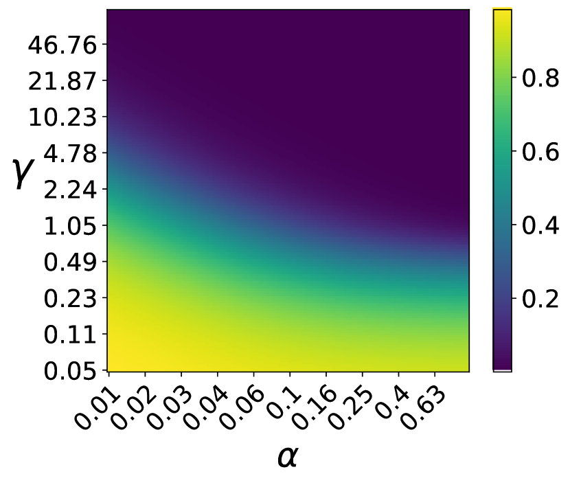
(a) $\textbf{Bias}^{2}$

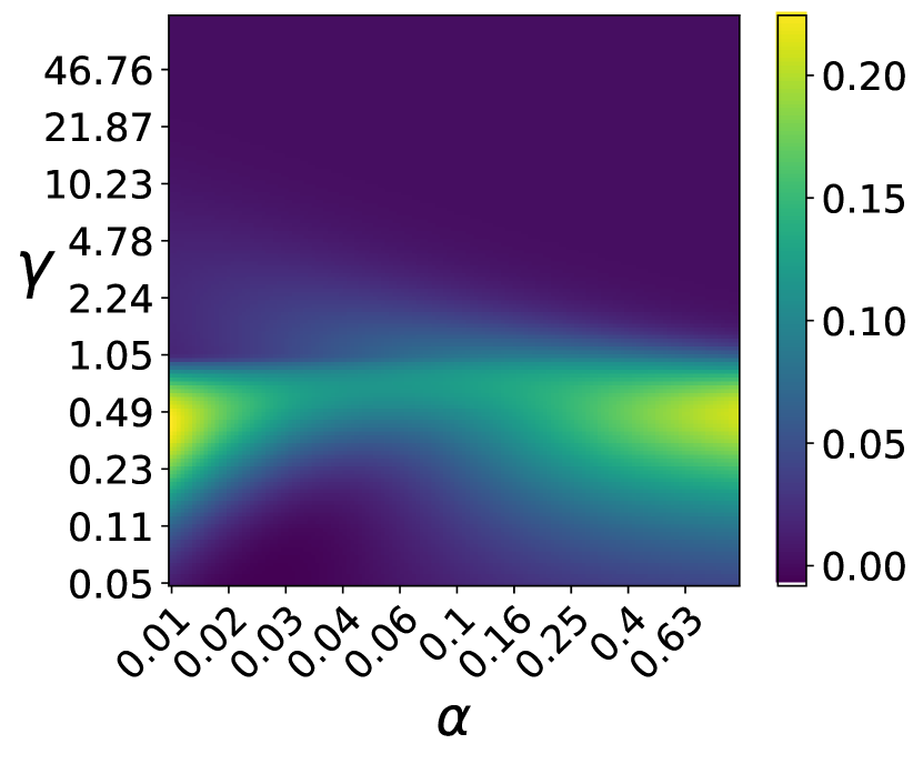
(b) $\textbf{Variance}_{\text{clean}}$

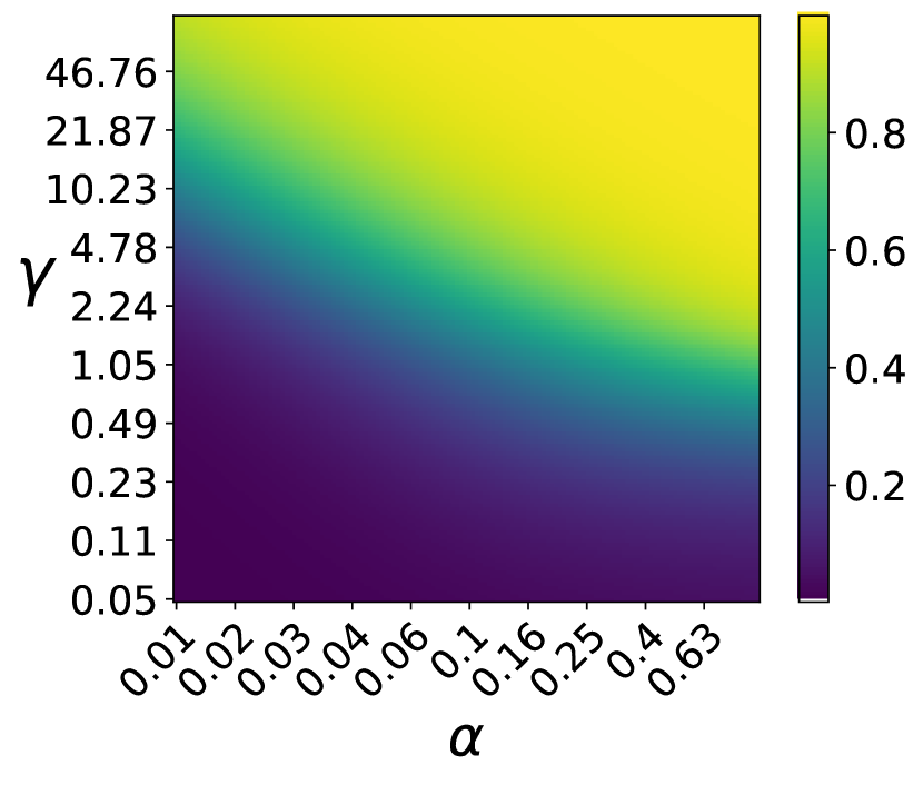
(c) $\textbf{Variance}_{\text{noise}}/\kappa$

Figure 13: Expressions of $\textbf{Bias}^{2}$, $\textbf{Variance}_{\text{clean}}$ and $\textbf{Variance}_{\text{noise}}/\kappa$ in Theorem 3.2

A.6 Variants of Theorem 3.2

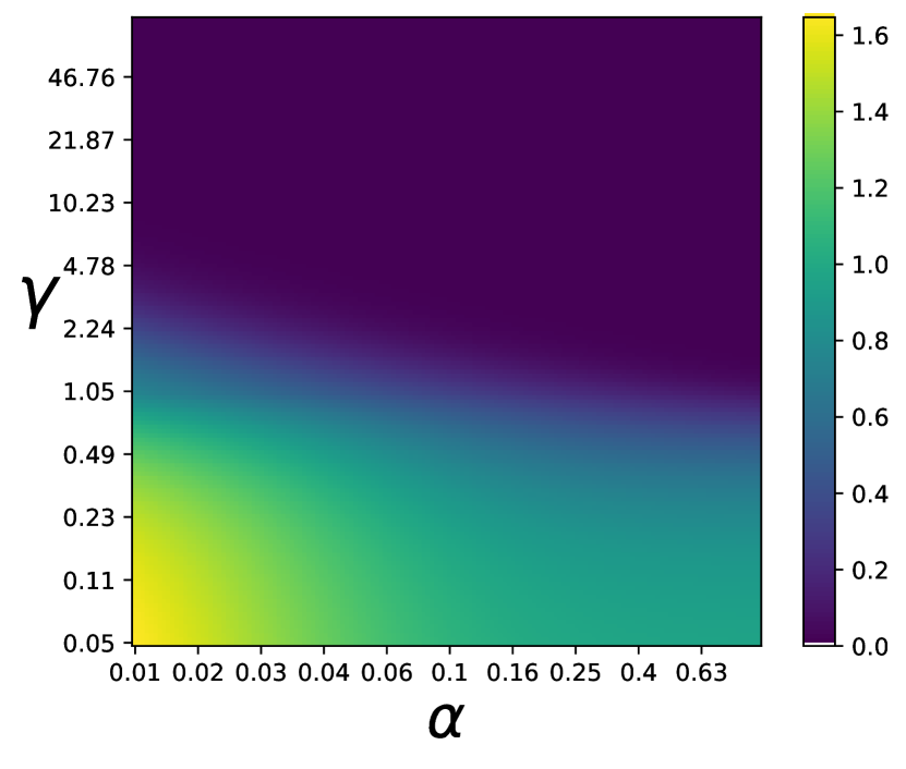
(a) Risk ($\kappa=0$)

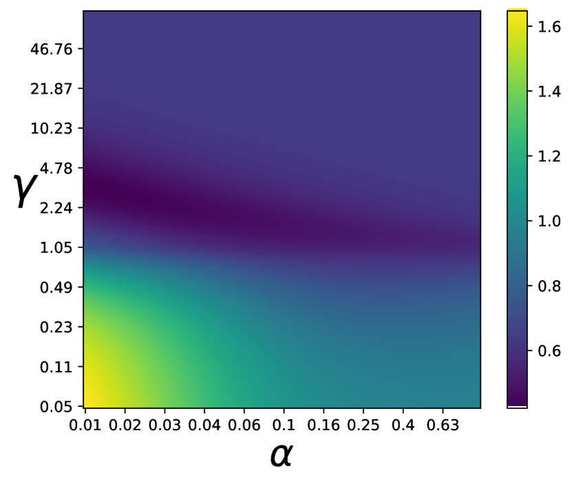
(b) Risk ($\kappa=0.64$)

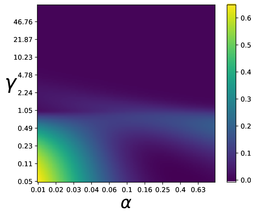
(c) Variance ($\kappa=0$)

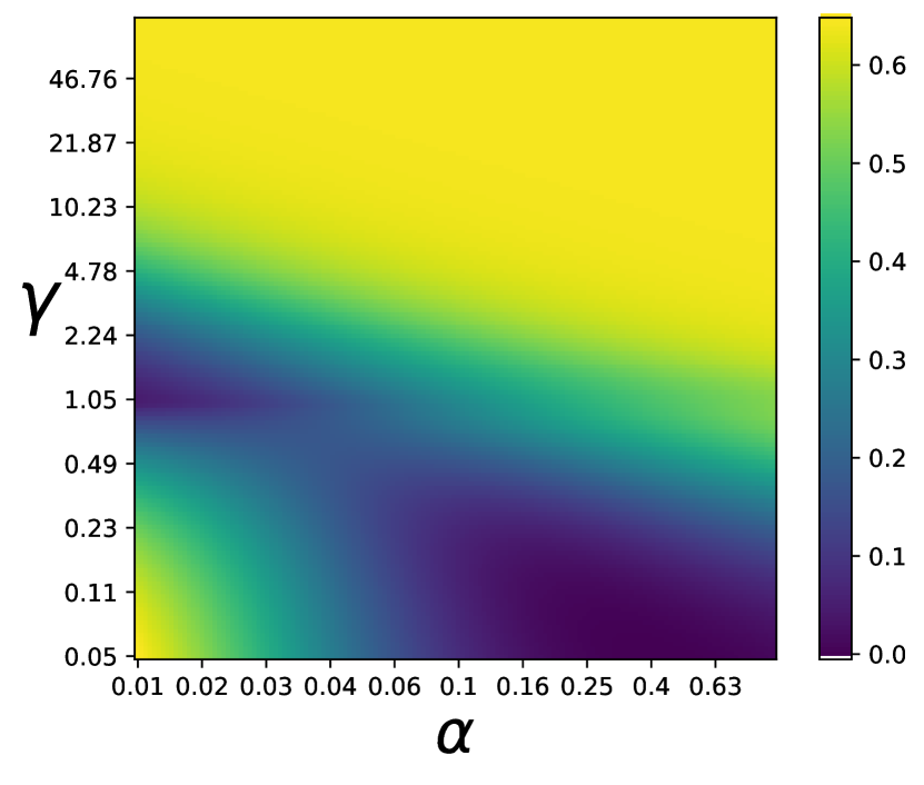
(d) Variance ($\kappa=0.64$)

Figure 14: Expressions of the risk and variance under different noise levels with $\tau=\gamma$. We let $\lambda_{0}=0.05$.

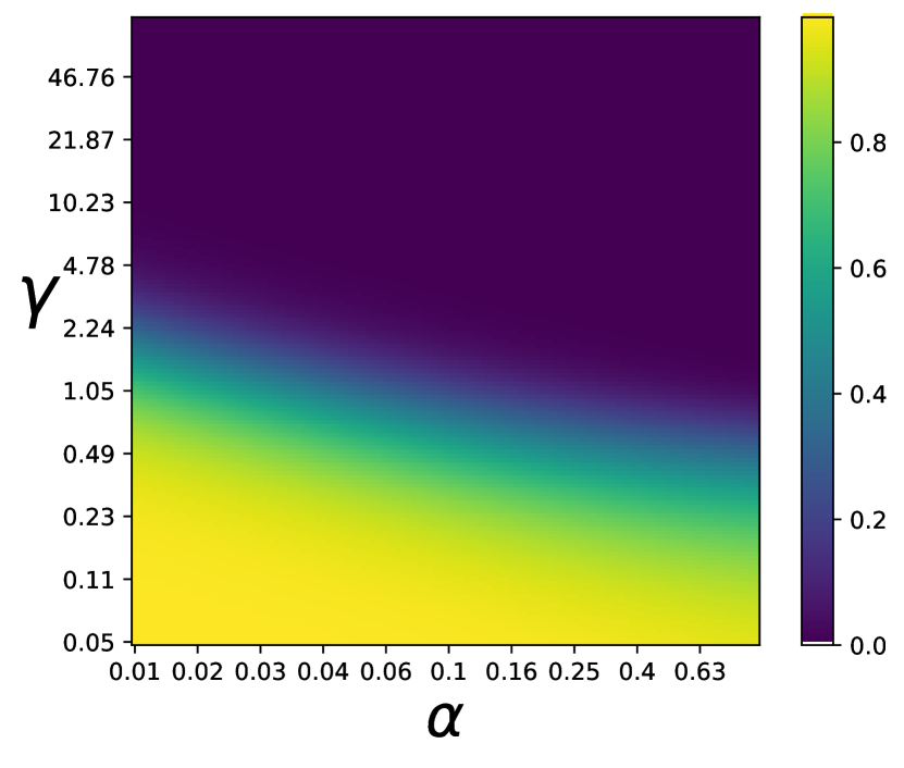
(a) $\textbf{Bias}^{2}$

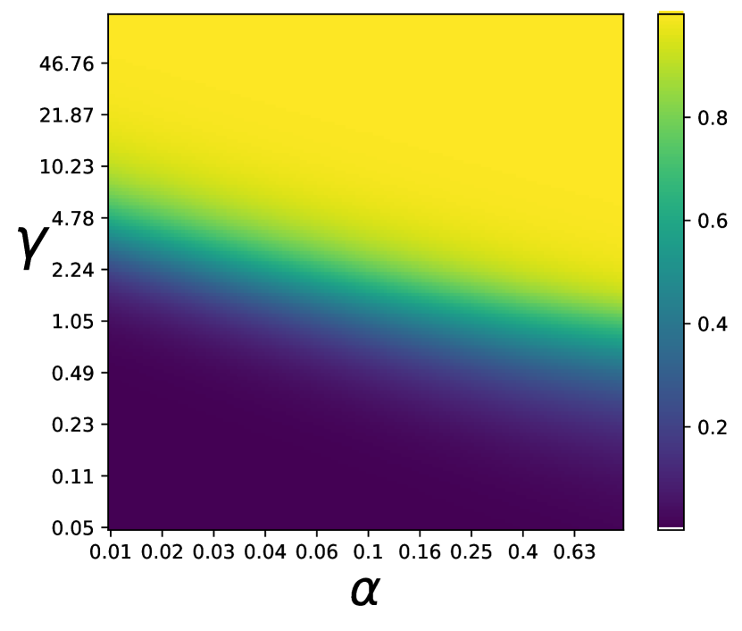
(b) $\textbf{Variance}_{\text{noise}}/\kappa$

Figure 15: Expressions of $\textbf{Bias}^{2}$ and $\textbf{Variance}_{\text{noise}}/\kappa$ with $\tau=\gamma$.

In Theorem 3.2 we let $\bm{\mu}$’s entries be drawn from $\mathcal{N}(0,1/q)$ so that $q$ does not appear in the expression of the risk. Alternatively we can let $\bm{\mu}$’s entries be drawn from $\mathcal{N}(0,1/d)$ and assume $q/d=\tau$. Then the risk and its decomposition are dependent on $\gamma,\tau,\alpha$. Similar to the proof in A.4, we can show that in this case we only have to replace $\lambda_{0}$ in the setting of Theorem 3.1 with $\lambda_{0}/(\tau\alpha)$ to get the expressions of risk. We further let $\tau=\gamma$ and plot the risk, Variance, $\textbf{Bias}^{2}$, $\textbf{Variance}_{\text{clean}}$ (i.e., Variance with $\kappa=0$), $\textbf{Variance}_{\text{noise}}$ in Figures 14 and 15.

A.7 Connection to the observation made by Golubeva et al. [2020]

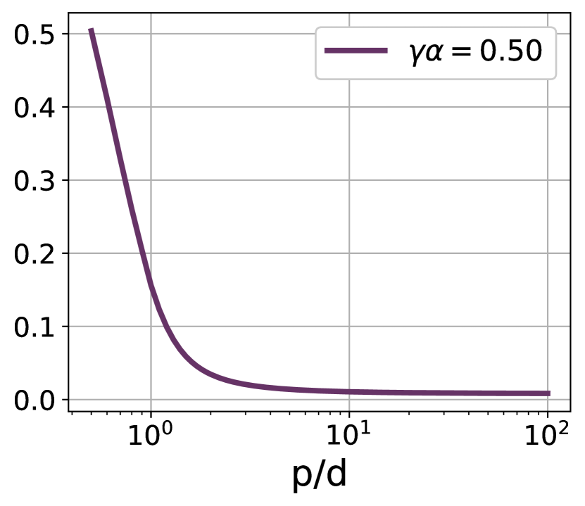
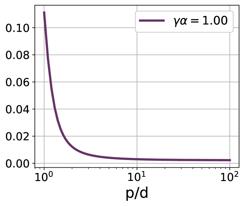
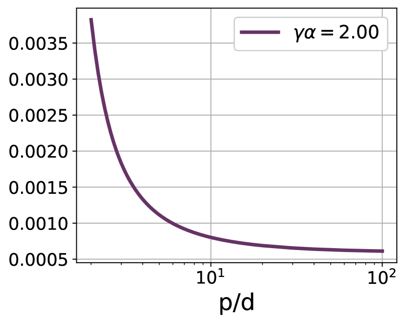
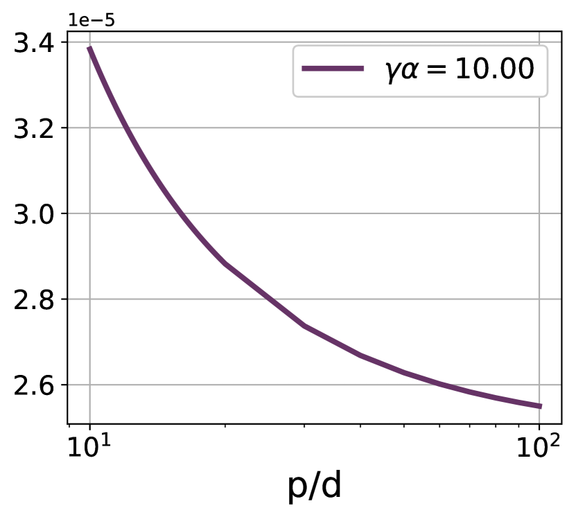
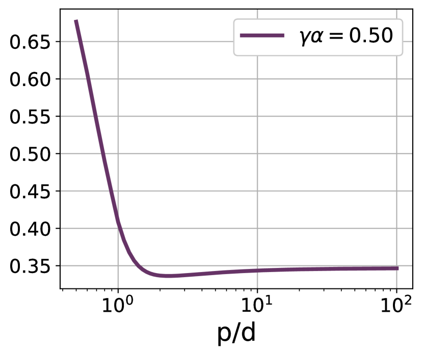
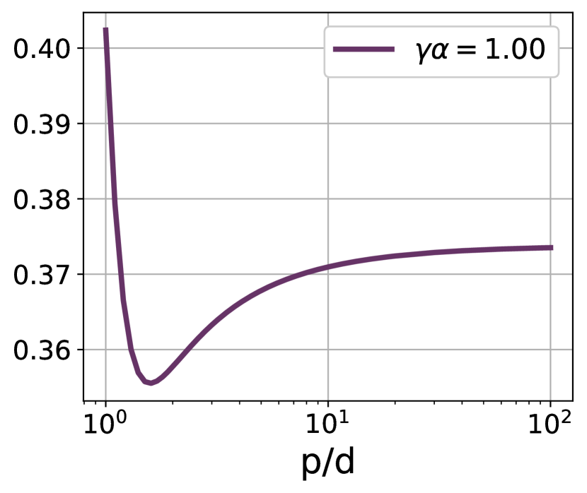
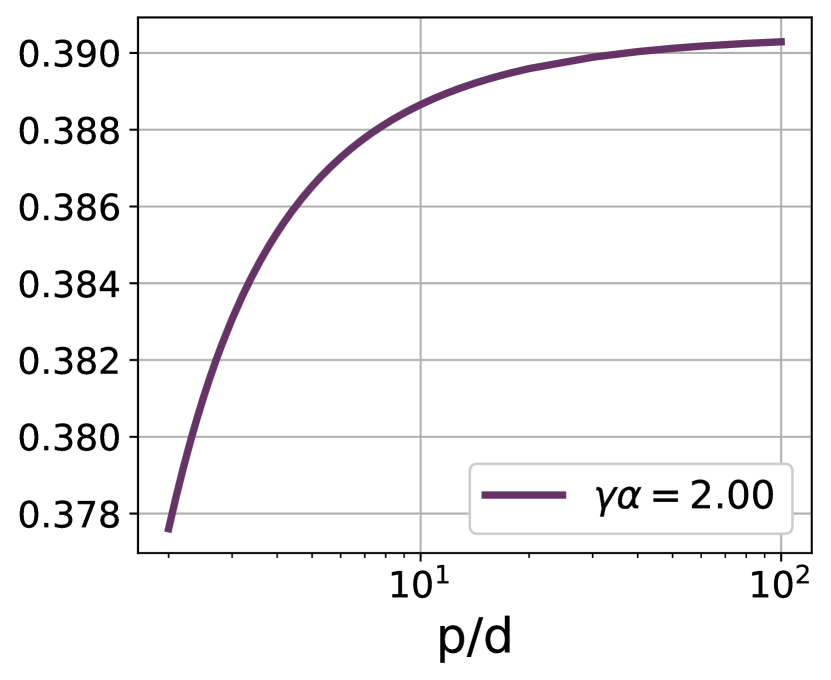
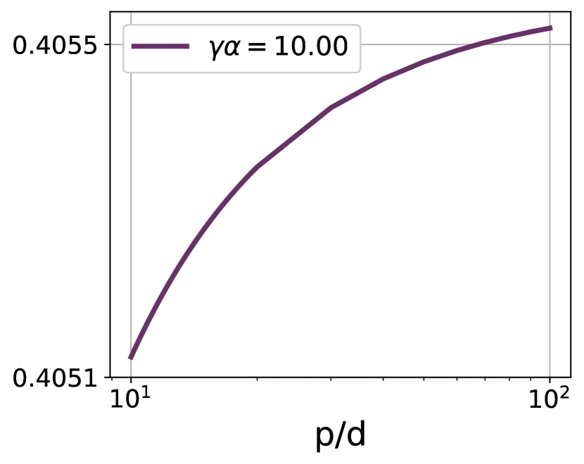
Figure 16: Risk curve with fixed $\gamma\alpha$. Top: $\kappa=0$, the test loss decreases with width. Bottom: $\kappa=0.64$, the test is either U-shaped or increasing.

Our Theorem 3.2 supports the empirical observation in Golubeva et al. [2020] that increasing width while fixing the number of parameters (by reducing density) improves generalization. This distinguishes the impact of width from the effect of increasing model capacity. In our experiments, we fix $\gamma\alpha$ and plot the risk curve with varying $\gamma$ (subject to $\alpha\leq 1$) in Figure 16. For $\kappa=0$, the test loss decreases with width. However, in the presence of large noise, the curve’s shape can be altered. For $\kappa=0.64$, the test loss exhibits either a U-shaped curve or an increasing trend.

Appendix B Additional Results for Random Feature Ridge Regression with Different $n/d$ Ratios

Figure 17 shows the shape of total variance when $\lambda=0.2$. Figures 18 and 19 show the shape of $\frac{1}{\sigma^{2}}\textbf{Variance}_{\text{noise}}$ with $\lambda=0.2$ and $0.01$, respectively.

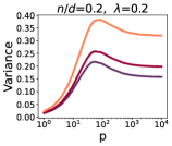
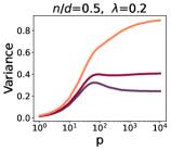
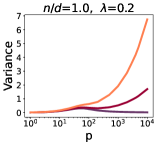
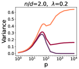
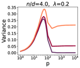
Figure 17: We plot the total variance in random feature ridge regression while fixing $d=100$ and $\lambda=0.2$, and varying $\sigma^{2}$. Legends show the values of $\sigma^{2}$, and titles show the values of $n/d$.

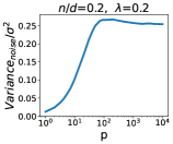
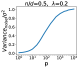
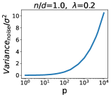
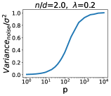
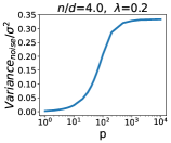
Figure 18: $\frac{1}{\sigma^{2}}\textbf{Variance}_{\text{noise}}$ under different values of $n/d$ with $\lambda=0.2$.

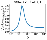
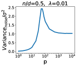
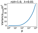
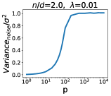
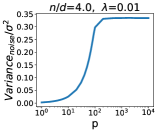
Figure 19: $\frac{1}{\sigma^{2}}\textbf{Variance}_{\text{noise}}$ under different values of $n/d$ with $\lambda=0.01$.

Appendix C Experimental Setting Details for Neural Networks

All experiments are implemented using PyTorch. We use eight Nvidia A40 to run the experiments.

C.1 Noise Types

Symmetric noise

Symmetric noise is generated by randomly shuffling the labels of certain fraction of examples.

Asymmetric noise

Asymmetric noise is class-dependent. We follow the scheme proposed in Patrini et al. [2017] which is also widely used in robust method papers (e.g., ELR Liu et al. [2020] and DivideMix Li et al. [2020]). For CIFAR-10, labels are randomly flipped according to the following map: TRUCK$\rightarrow$AUTOMOBILE, BIRD$\rightarrow$AIRPLANE, DEER$\rightarrow$HORSE, CAT$\rightarrow$DOG, DOG$\rightarrow$CAT. For CIFAR-100, since the 100 classes are grouped into 20 superclasses, e.g. AQUATIC MAMMALS contains BEAVER, DOLPHIN, OTTER, SEAL and WHALE, we flip labels of each class into the next one circularly within super-classes. For both datasets, the fraction of mislabeled examples in the training set is the noise level.

Web Noise

Red Stanford Car Jiang et al. [2020] contains images crawled from web, with label noise introduced through text-to-image and image-to-image search. There are 10 different noise levels {0%, 5% 10%, 15%, 20%, 30%, 40%, 60%, 80%} for this dataset and we choose 40% and 80%. For each noise level, the mislabeled web images can only be downloaded from the provided URLs. The training splits and labels are in provided files . The original dataset size is 8144. For 80% noise, there are 6469 web images. However, 590 of the URL links are not functional and among the downloaded JPG files 1871 are corrupted/unopenable, hence we end up with 1675 clean examples and 4008 noisy examples, i.e., the actual noise level is 70.53%. For 40% noise, there are 3241 web images with 313 non-downloadable and 963 not unopenable. Therefore the actual noise level is 29.03%.

C.2 Empirically Measuring Bias and Variance

To empirically examine the transition in variance shape as suggested by Theorem 3.1, we adopt the unbiased estimator proposed in Yang et al. [2020]. Specifically, we randomly divide the training set for each model into $N$ subsets (with $N=20$ for MNIST and $N=5$ for CIFAR-10). For each subset, we train a separate model and compute the variance of the network output across these subsets. We use the mean squared error (MSE) loss on both datasets, as the bias-variance decomposition is only well-defined for MSE (refer to Eq. 1). While Yang et al. [2020] also proposed an estimator for cross-entropy loss, it is biased and may introduce skewed results.

C.3 Training Details for Sections 4.2 and 4.3

We see weight decay and $\ell_{2}$ regularization as equivalent terms. Thus, when we specify $\lambda=0.001$, it indicates that we employ a weight decay value of 0.001. The width of a two-layer network is controlled by the number of hidden neurons. The width of a ResNet is controlled by the number of convolutional layer filters: for width $w$, there are $w$, $2w$, $4w$, $8w$ filters in each layer of the four Residual Blocks, respectively. When reducing the density of a model, we randomly select a certain fraction of its weights and then keep them zero throughout the training.

MNIST and CIFAR-10 with MSE loss and Symmetric noise. We train two-layer ReLU networks on MNIST and ResNet34 on CIFAR-10. On MNIST, we train each model for 200 epochs using SGD with batch size 64, momentum 0.9, initial learning rate 0.1, learning rate decay of 0.1 every 50 epochs. On CIFAR-10 we train each model for 1000 epochs using SGD with batch size 128, momentum 0.9, initial learning rate 0.1, learning rate decay of 0.1 every 400 epochs.

CIFAR-10/100 with CE loss and Asymmetric/Symmetric noise On both datasets, we train ResNet34 for 500 epochs using SGD with batch size 128, momentum 0.9, initial learning rate 0.1, learning rate decay of 0.1 every 100 epochs.

InceptionResNet-v2 on Red Stanford Car We train each model for 160 epochs with an initial learning rate of 0.1, and a weight decay of $1\times 10^{-5}$ using SGD and momentum of 0.9 with a batch size of 32. We anneal the learning rate by a factor of 10 at epochs 80 and 120, respectively. We use Cross Entropy loss.

C.4 Training Details for Section 4.4

ELR leverages the early learning phenomenon where the network fits clean examples first and then mislabeled examples. It hinders learning wrong labels by regularizing the loss with a term that encourages the alignment between the model’s prediction and the running average of the predictions in previous rounds. DivideMix dynamically discards labels that are highly likely to be noisy and trains the model in a semi-supervised manner. For both ELR and DivideMix we use the same setup as in the original papers Liu et al. [2020], Li et al. [2020].

ELR We train ResNet-34 using SGD with momentum 0.9, a weight decay of 0.001, and a batch size of 128. The network is trained for 120 epochs on CIFAR-10 and 150 epochs on CIFAR-100. The learning rate is 0.02 at initialization, and decayed by a factor of 100 at epochs 40 and 80 for CIFAR-10 and at epochs 80 and 120 for CIFAR-100. We use $0.7$ for the temporal ensembling parameter, and $3$ for the ELR regularization coefficient.

DivideMix We train ResNet-34 for 200 epochs using SGD with batch size $64$, momentum $0.9$, initial learning rate $0.02$, a weight decay of $5\times 10^{-4}$, and a learning rate decay of $0.1$ at epoch 150. We use $150$ for the unsupervised loss weight.

Appendix D Additional Experimental Results for Section 4

D.1 Effect of Width

Additional results for Figures 6 and 7. Test accuracy, $\textbf{Bias}^{2}$ and Variance are shown in Figures 20 to 23.

Effect of Sample Size. We use MSE loss on MNIST and CE loss on CIFAR-10. We consider $\lambda=0.001$ and 60% noise for both datasets. Plots of test accuracy are shown in Figure 24.

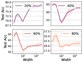
(a)

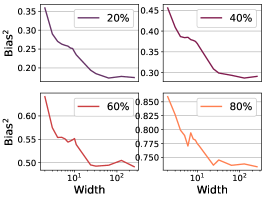
(b)

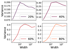
(c)

Figure 20: CIFAR-10, MSE loss, $\lambda=0.0005$

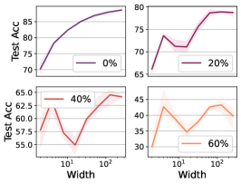
(a)

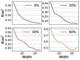
(b)

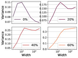
(c)

Figure 21: CIFAR-10, MSE loss, $\lambda=0.001$

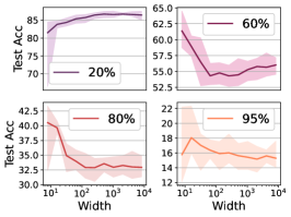
(a)

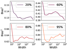
(b)

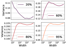
(c)

Figure 22: MNIST, MSE loss, $\lambda=0$

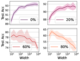
(a)

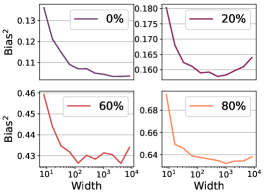
(b)

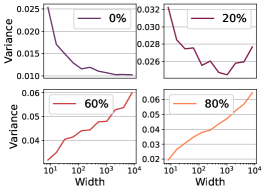
(c)

Figure 23: MNIST, MSE loss, $\lambda=0.001$

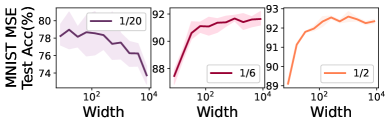
(a)

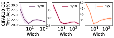
(b)

Figure 24: We plot test accuracy against width while varying sample size. We use MSE loss with $\lambda=0.001$ on MNIST and CE loss with $\lambda=0.001$ on CIFAR-10.

D.2 Effect of Density

Joint effect of width and density When studying the joint effect of width and density, we utilize MSE loss to measure bias and variance. We set $\lambda=0$ for MNIST and $\lambda=0.0005$ for CIFAR-10. The results are presented in Figures 11, 25, and 26. In both settings, models with the smallest density achieve the highest accuracy, and models with very small density achieve the optimal loss.

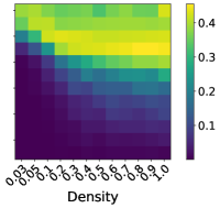
Figure 25: Variance under varied width and density on CIFAR-10.

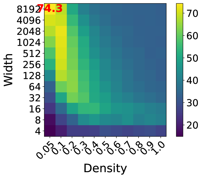
(a) Test Acc. (MNIST)

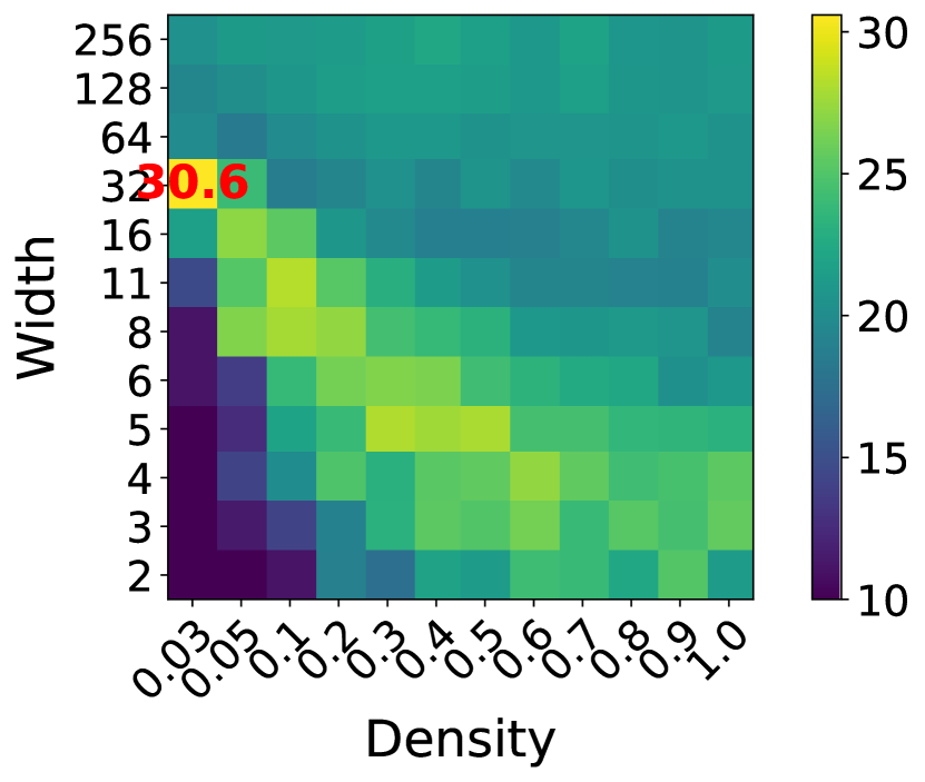
(b) Test Acc. (CIFAR-10)

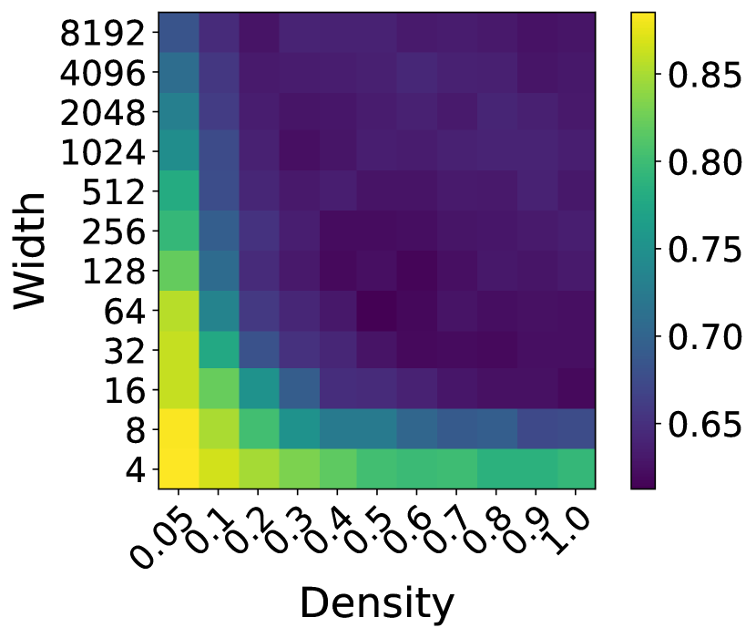
(c) $\textbf{Bias}^{2}$ (MNIST)

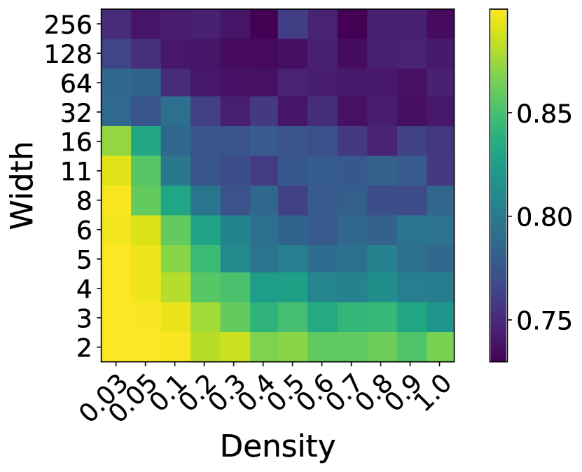
(d) $\textbf{Bias}^{2}$ (CIFAR-10)

Figure 26: Test accuracy and bias under varied width and density. Red numbers show the highest accuracy.

Smaller density vs. stronger $l_{2}$ regularization We train ResNet34 with a width of 16 on CIFAR-10, using 50% symmetric noise. We compare the results obtained by varying $\lambda$ (weight decay) and by varying the model density. Figure 11(d) shows the test loss and 27 shows the test accuracy.

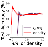
Figure 27: Test accuracy obtained by varying $\lambda$ (weight decay) or by varying model density.

D.3 When Robust Methods are Applied

In addition to the experiments presented in the main paper, we provide results for the following experiments conducted on CIFAR-10/100: width experiments with ELR under 80% noise (Figure 28), density experiments with ELR (Figure 29), density experiments with DivideMix under 60% noise (Figure 30). Furthermore, we show the results of density experiments on Red Stanford Car with 70% noise, where InceptionResNet-v2 is trained using ELR in Figure 31. In the plots, the purple solid line represents test loss and the blue dashed line represents test accuracy.

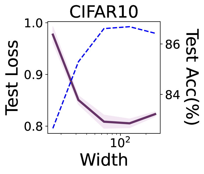
(a) ELR, Sym, 60%

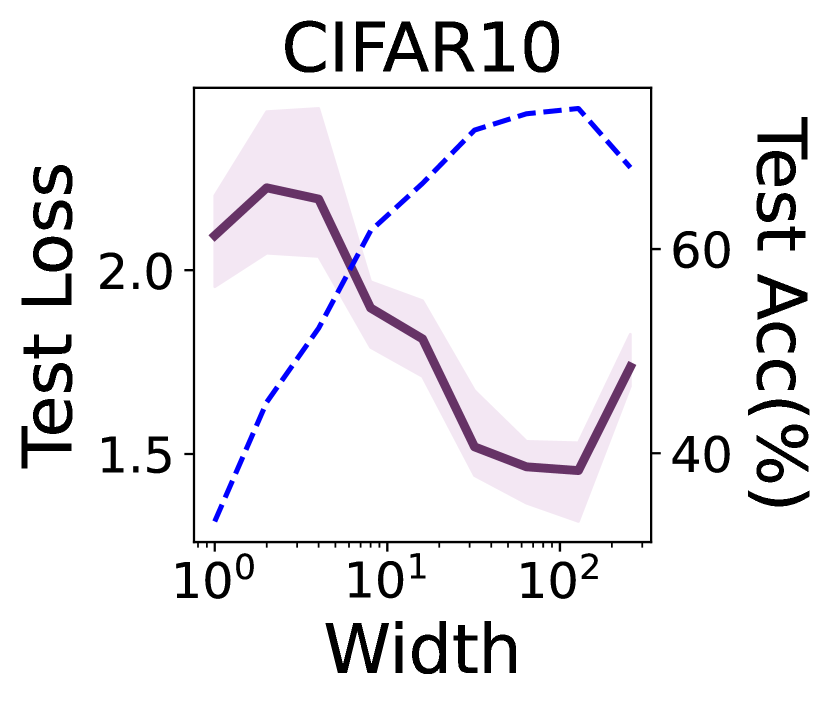
(b) ELR, Sym, 80%

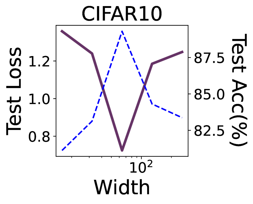
(c) ELR, Asym, 35%

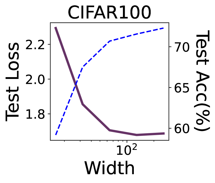
(d) ELR, Sym, 30%

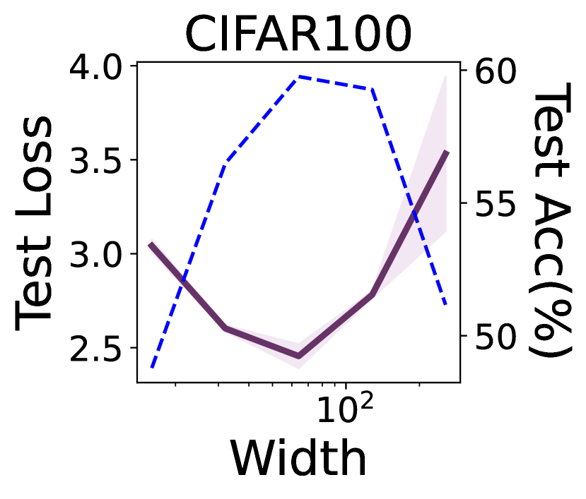
(e) ELR, Sym, 60%

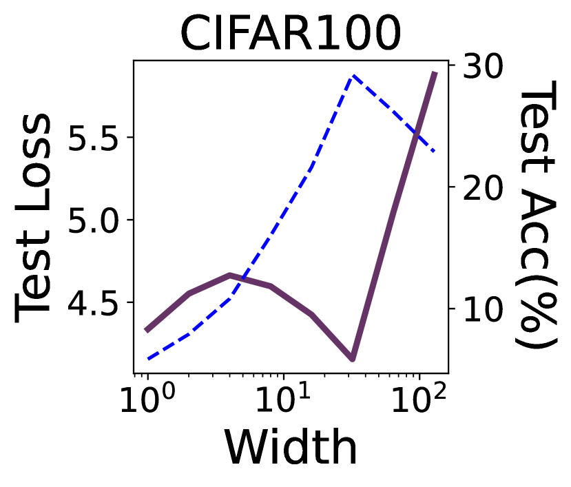
(f) ELR, Sym, 80%

Figure 28: Additional results for the effect of width when ELR is used. The top row displays the results on CIFAR-10, and the bottom row displays the results on CIFAR-100.

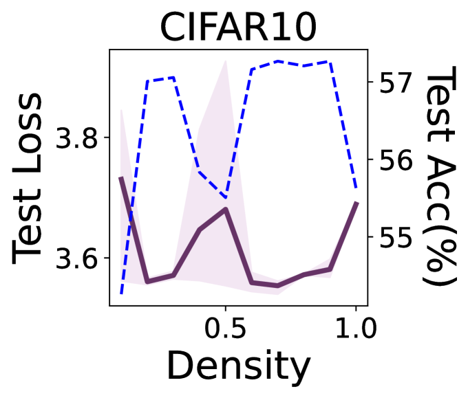
(a) C10, Asym 30%, width 128

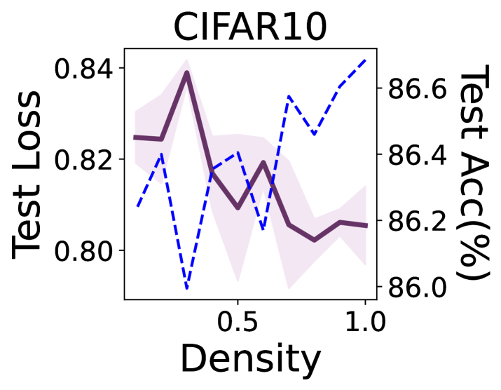
(b) C10, Sym 60%, width 128

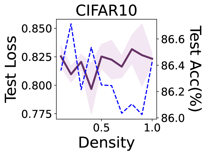
(c) C10, Sym 60%, width 256

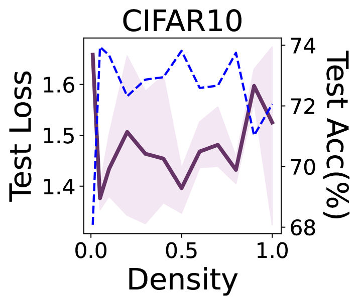
(d) C10, Sym 80%, width 128

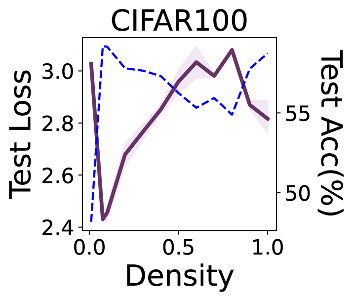
(e) C100, Sym 60%, width 128

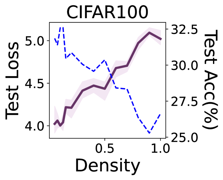
(f) C100, Sym 80%, width 64

Figure 29: Effect of density when ELR is used.

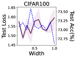
Figure 30: Effect of density when DivideMix is used. We train the model on CIFAR-100 and set width to 64.

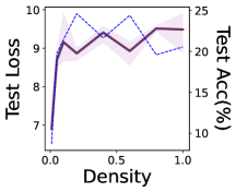
Figure 31: Effect of density when we train an InceptionResNetV2 on Red Stanford Cars.

Appendix E Investigating the Complexity of Learned Functions

A hypothesis proposed by Belkin et al. [2019] for double descent suggests that the learning algorithm possesses the right inductive bias towards "low complexity" functions that generalize well while fitting the training set. It posits that larger model sizes, which correspond to richer function classes, provide the algorithm with more choices to discover functions with lower complexity. Given our finding that large noise alters the correlation between model size and generalization, a natural question arises: "Does large noise also change the correlation between model size and the complexity of learned functions?" In this section, we present empirical evidence suggesting the possibility of an affirmative answer. Recently, Kalimeris et al. [2019] qualitatively measured the complexity of neural networks based on how much their predictions could be explained by a smaller model. However, this approach assumes that "smaller models have lower complexity," which may not hold in our case. Instead, we consider the following three measures:

• Trajectory length of the first layers bias. $\sum_{t\in T}\frac{\|\bm{b}_{1}^{(t+1)}-\bm{b}_{1}^{t}\|_{2}}{\alpha_{t}\epsilon_{f^{(t)}}}$ where $T$ is a set of iteration indices, $\bm{b}_{1}^{(t)}$ is the parameter of the first layer bias at iteration $t$, and $\epsilon_{f^{(t)}}$ is the gradient of the loss w.r.t. the network’s output at epoch $t$. Loukas et al. [2021] shows that, under certain conditions, the above can be both upper and lower bounded in terms of the Lipschitz constants of functions represented by the network at iterations in $T$ (see their Theorem 1). This implies that the first layer bias travels longer during training when it is fitting a more complex function.

• Variance of the first layer bias $\text{avg}_{t\in T}\|\bm{b}_{1}^{(t)}-\text{avg}_{t\in T}\bm{b}_{1}^{(t)}\|_{2}^{2}$. Loukas et al. [2021] also provides a lower bound for the above in terms of the Lipschitz constant and $\epsilon_{f^{(t)}}$ (their Corollary 2). Thus a larger Lipschitz constant leads to a higher lower bound, meaning that when fitting a lower complexity function, the network’s bias will update more frequently during training.

• Product of spectral norms of the layer parameters. This is known as an upper bound for the network’s Lipschitz constant Szegedy et al. [2013]. For convolutional layers, the spectral norm is computed using the FFT-based algorithm in Sedghi et al. [2018].

Our experimental setup is the same as that of Loukas et al. [2021] (Task 2 in Section 6). We train CNNs on CIFAR-10 DOG vs AIRPLANE. The CNN consists of one identity layer, two convolutional layers with a kernel size of 5, a fully connected ReLU layer with a size of 384, and a linear layer. The width of the CNN is controlled by the number of convolutional channels, with $16w$ channels in each convolutional layer for width $w$. We employ binary cross-entropy (BCE) loss and train the models for 200 epochs using vanilla SGD with a batch size of 1. We apply exponential learning rate decay with a factor of $10^{-50}$. The trajectory length and variance are computed at every epoch, reflecting the complexity of the CNN’s represented function at each stage. The results are depicted in Figure 32, showing that noise can alter the relative complexity of functions learned by models with increasing width or density. This trend is more pronounced in the case of width (Figures 32(a) and 32(c)), where both quantities decrease under 0% noise and increase under 40% noise as width increases. Figure 33 presents the product of layer-wise spectral norms of the neural network at the final epoch, showing a similar pattern. These results suggests that label noise can invert the originally negative correlation between size and complexity/smoothness.

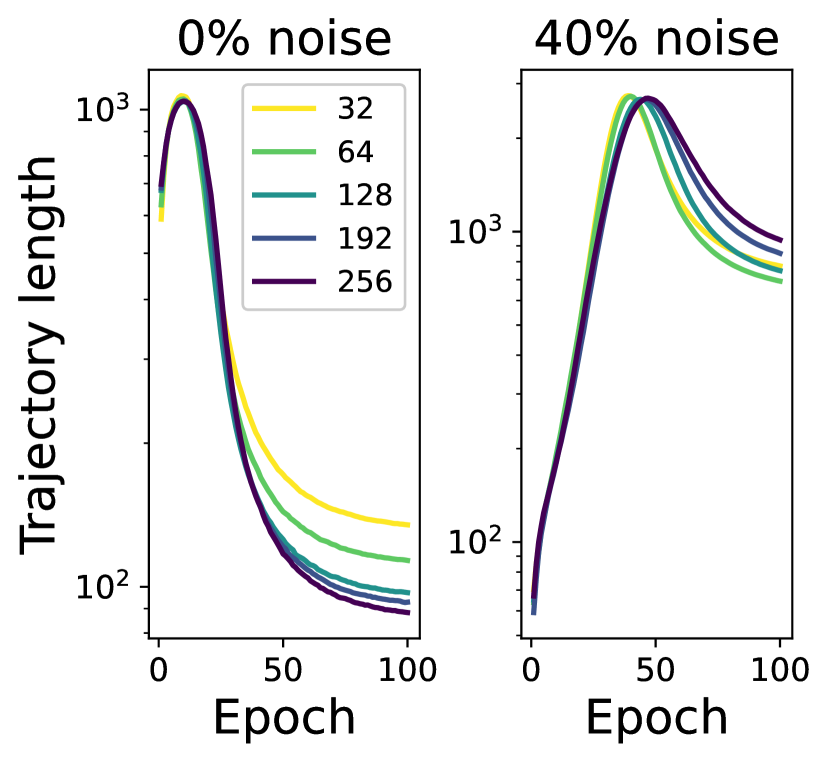
(a) Trajectory, width

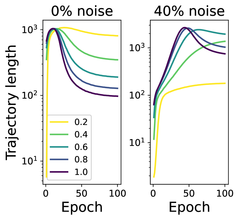
(b) Trajectory, density

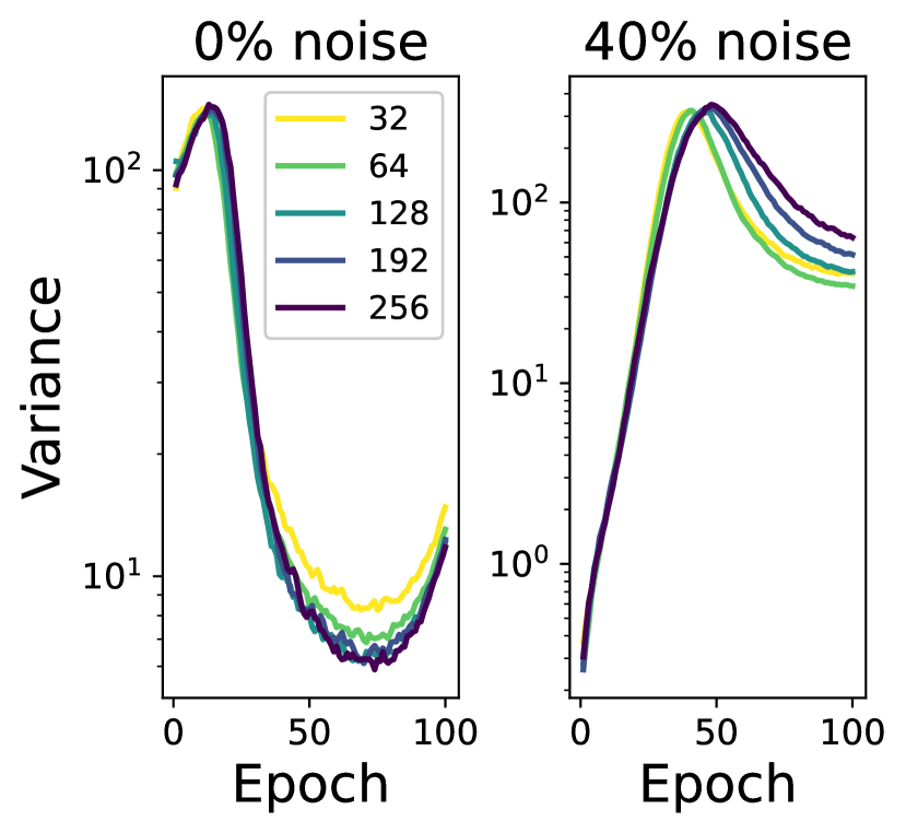
(c) Variance, width

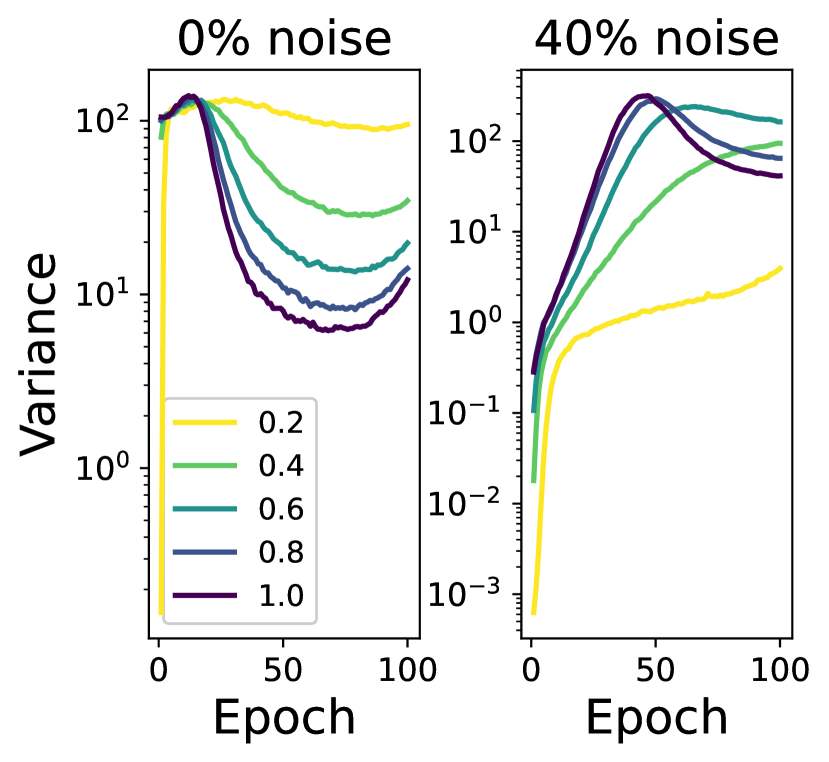
(d) Variance, density

Figure 32: Trajectory length and variance of the first layer bias during each epoch. When varying the density we fix the width to 128.

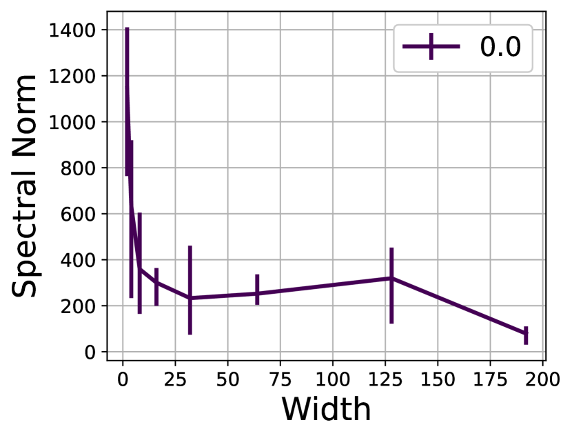
(a) 0% noise, width

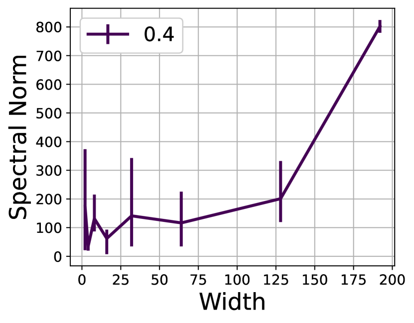
(b) 40% noise, width

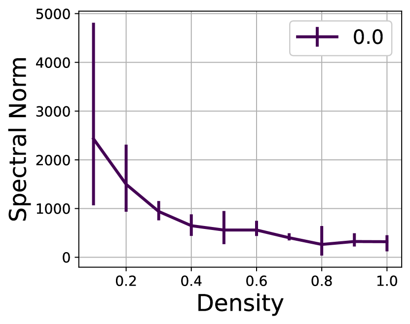
(c) 0% noise, density

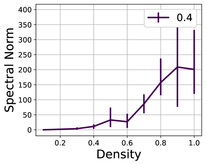
(d) 40% noise, density

Figure 33: When width or density increases, spectral norm decreases under 0% noise but increases under 40% noise.

Appendix F Potential Connection to Benign/Catastrophic Overfitting

The term ‘benign overfitting’ describes the phenomenon where models trained to overfit the training set still achieve nearly optimal generalization performance Bartlett et al. [2020], Tsigler and Bartlett [2020], Chatterji et al. [2021], Cao et al. [2022], Frei et al. [2022], Mallinar et al. [2022]. Recently, Cao et al. [2022] demonstrated that sufficiently large models exhibit benign overfitting when the product of sample size and signal-to-noise ratio (SNR) is large, and catastrophic overfitting occurs otherwise. Notably, this condition coincides with the condition in our theory (Section 3) where the final ascent does not occur, since the SNR is represented as $1/\sigma^{2}$ in our setting. Consequently, our findings can be interpreted in the context of benign/catastrophic overfitting: when the noise-to-sample-size ratio is large, a ‘sufficiently large’ model overfits catastrophically, implying that increasing the model size towards a sufficient extent may worsen generalization. Indeed, neural networks and various other real interpolating methods typically operate in the ‘tempered overfitting’ regime Mallinar et al. [2022]. Our results suggest that the condition for benign overfitting identified in Cao et al. [2022] can potentially be extended to assess the relative ‘benignity’ of tempered overfitting across different model sizes. The theoretical establishment of this connection could be a valuable direction for future research.

References

- Devlin et al. (2018) Jacob Devlin, Ming-Wei Chang, Kenton Lee, and Kristina Toutanova. Bert: Pre-training of deep bidirectional transformers for language understanding. arXiv preprint arXiv:1810.04805, 2018.
- Dosovitskiy et al. (2020) Alexey Dosovitskiy, Lucas Beyer, Alexander Kolesnikov, Dirk Weissenborn, Xiaohua Zhai, Thomas Unterthiner, Mostafa Dehghani, Matthias Minderer, Georg Heigold, Sylvain Gelly, et al. An image is worth 16x16 words: Transformers for image recognition at scale. arXiv preprint arXiv:2010.11929, 2020.
- Brown et al. (2020) Tom Brown, Benjamin Mann, Nick Ryder, Melanie Subbiah, Jared D Kaplan, Prafulla Dhariwal, Arvind Neelakantan, Pranav Shyam, Girish Sastry, Amanda Askell, et al. Language models are few-shot learners. Advances in neural information processing systems, 33:1877–1901, 2020.
- Radford et al. (2021) Alec Radford, Jong Wook Kim, Chris Hallacy, Aditya Ramesh, Gabriel Goh, Sandhini Agarwal, Girish Sastry, Amanda Askell, Pamela Mishkin, Jack Clark, et al. Learning transferable visual models from natural language supervision. In International conference on machine learning, pages 8748–8763. PMLR, 2021.
- Krishna et al. (2016) Ranjay A Krishna, Kenji Hata, Stephanie Chen, Joshua Kravitz, David A Shamma, Li Fei-Fei, and Michael S Bernstein. Embracing error to enable rapid crowdsourcing. In Proceedings of the 2016 CHI conference on human factors in computing systems, pages 3167–3179, 2016.
- Belkin et al. (2019) Mikhail Belkin, Daniel Hsu, Siyuan Ma, and Soumik Mandal. Reconciling modern machine-learning practice and the classical bias–variance trade-off. Proceedings of the National Academy of Sciences, 116(32):15849–15854, 2019.
- Spigler et al. (2019) Stefano Spigler, Mario Geiger, Stéphane d’Ascoli, Levent Sagun, Giulio Biroli, and Matthieu Wyart. A jamming transition from under-to over-parametrization affects generalization in deep learning. Journal of Physics A: Mathematical and Theoretical, 52(47):474001, 2019.
- Yang et al. (2020) Zitong Yang, Yaodong Yu, Chong You, Jacob Steinhardt, and Yi Ma. Rethinking bias-variance trade-off for generalization of neural networks. In International Conference on Machine Learning, pages 10767–10777. PMLR, 2020.
- Adlam and Pennington (2020a) Ben Adlam and Jeffrey Pennington. Understanding double descent requires a fine-grained bias-variance decomposition. Advances in neural information processing systems, 33:11022–11032, 2020a.
- Liu et al. (2020) Sheng Liu, Jonathan Niles-Weed, Narges Razavian, and Carlos Fernandez-Granda. Early-learning regularization prevents memorization of noisy labels. Advances in neural information processing systems, 33:20331–20342, 2020.
- Li et al. (2020) Junnan Li, Richard Socher, and Steven CH Hoi. Dividemix: Learning with noisy labels as semi-supervised learning. arXiv preprint arXiv:2002.07394, 2020.
- LeCun (1998) Yann LeCun. The mnist database of handwritten digits. http://yann. lecun. com/exdb/mnist/, 1998.
- He et al. (2016) Kaiming He, Xiangyu Zhang, Shaoqing Ren, and Jian Sun. Deep residual learning for image recognition. In Proceedings of the IEEE conference on computer vision and pattern recognition, pages 770–778, 2016.
- Krizhevsky et al. (2009) Alex Krizhevsky, Geoffrey Hinton, et al. Learning multiple layers of features from tiny images. 2009.
- Szegedy et al. (2017) Christian Szegedy, Sergey Ioffe, Vincent Vanhoucke, and Alexander A Alemi. Inception-v4, inception-resnet and the impact of residual connections on learning. In Thirty-first AAAI conference on artificial intelligence, 2017.
- Jiang et al. (2020) Lu Jiang, Di Huang, Mason Liu, and Weilong Yang. Beyond synthetic noise: Deep learning on controlled noisy labels. In International Conference on Machine Learning, pages 4804–4815. PMLR, 2020.
- Neyshabur et al. (2014) Behnam Neyshabur, Ryota Tomioka, and Nathan Srebro. In search of the real inductive bias: On the role of implicit regularization in deep learning. arXiv preprint arXiv:1412.6614, 2014.
- Belkin et al. (2020) Mikhail Belkin, Daniel Hsu, and Ji Xu. Two models of double descent for weak features. SIAM Journal on Mathematics of Data Science, 2(4):1167–1180, 2020.
- Derezinski et al. (2020) Michal Derezinski, Feynman T Liang, and Michael W Mahoney. Exact expressions for double descent and implicit regularization via surrogate random design. Advances in neural information processing systems, 33:5152–5164, 2020.
- Kuzborskij et al. (2021) Ilja Kuzborskij, Csaba Szepesvári, Omar Rivasplata, Amal Rannen-Triki, and Razvan Pascanu. On the role of optimization in double descent: A least squares study. Advances in Neural Information Processing Systems, 34, 2021.
- Hastie et al. (2019) Trevor Hastie, Andrea Montanari, Saharon Rosset, and Ryan J Tibshirani. Surprises in high-dimensional ridgeless least squares interpolation. arXiv preprint arXiv:1903.08560, 2019.
- Mei and Montanari (2019) Song Mei and Andrea Montanari. The generalization error of random features regression: Precise asymptotics and the double descent curve. Communications on Pure and Applied Mathematics, 2019.
- d’Ascoli et al. (2020) Stéphane d’Ascoli, Maria Refinetti, Giulio Biroli, and Florent Krzakala. Double trouble in double descent: Bias and variance (s) in the lazy regime. In International Conference on Machine Learning, pages 2280–2290. PMLR, 2020.
- Adlam and Pennington (2020b) Ben Adlam and Jeffrey Pennington. The neural tangent kernel in high dimensions: Triple descent and a multi-scale theory of generalization. volume 119. PMLR, 2020b.
- Nakkiran et al. (2021) Preetum Nakkiran, Gal Kaplun, Yamini Bansal, Tristan Yang, Boaz Barak, and Ilya Sutskever. Deep double descent: Where bigger models and more data hurt. Journal of Statistical Mechanics: Theory and Experiment, 2021(12):124003, 2021.
- Frankle and Carbin (2018) Jonathan Frankle and Michael Carbin. The lottery ticket hypothesis: Finding sparse, trainable neural networks. arXiv preprint arXiv:1803.03635, 2018.
- Lee et al. (2018) Namhoon Lee, Thalaiyasingam Ajanthan, and Philip HS Torr. Snip: Single-shot network pruning based on connection sensitivity. arXiv preprint arXiv:1810.02340, 2018.
- Frankle et al. (2019) Jonathan Frankle, Gintare Karolina Dziugaite, Daniel M Roy, and Michael Carbin. Stabilizing the lottery ticket hypothesis. arXiv preprint arXiv:1903.01611, 2019.
- Wang et al. (2020) Chaoqi Wang, Guodong Zhang, and Roger Grosse. Picking winning tickets before training by preserving gradient flow. arXiv preprint arXiv:2002.07376, 2020.
- Frankle et al. (2020) Jonathan Frankle, Gintare Karolina Dziugaite, Daniel M Roy, and Michael Carbin. Pruning neural networks at initialization: Why are we missing the mark? arXiv preprint arXiv:2009.08576, 2020.
- Tanaka et al. (2020) Hidenori Tanaka, Daniel Kunin, Daniel L Yamins, and Surya Ganguli. Pruning neural networks without any data by iteratively conserving synaptic flow. Advances in Neural Information Processing Systems, 33:6377–6389, 2020.
- Jin et al. (2022) Tian Jin, Michael Carbin, Daniel M Roy, Jonathan Frankle, and Gintare Karolina Dziugaite. Pruning’s effect on generalization through the lens of training and regularization. arXiv preprint arXiv:2210.13738, 2022.
- Renda et al. (2020) Alex Renda, Jonathan Frankle, and Michael Carbin. Comparing rewinding and fine-tuning in neural network pruning. arXiv preprint arXiv:2003.02389, 2020.
- Zhang and Sabuncu (2018) Zhilu Zhang and Mert Sabuncu. Generalized cross entropy loss for training deep neural networks with noisy labels. In Advances in neural information processing systems, pages 8778–8788, 2018.
- Jiang et al. (2018) Lu Jiang, Zhengyuan Zhou, Thomas Leung, Li-Jia Li, and Li Fei-Fei. Mentornet: Learning data-driven curriculum for very deep neural networks on corrupted labels. In International Conference on Machine Learning, pages 2309–2318, 2018.
- Han et al. (2018) Bo Han, Quanming Yao, Xingrui Yu, Gang Niu, Miao Xu, Weihua Hu, Ivor Tsang, and Masashi Sugiyama. Co-teaching: Robust training of deep neural networks with extremely noisy labels. In Advances in neural information processing systems, pages 8527–8537, 2018.
- Mirzasoleiman et al. (2020) Baharan Mirzasoleiman, Kaidi Cao, and Jure Leskovec. Coresets for robust training of deep neural networks against noisy labels. Advances in Neural Information Processing Systems, 33, 2020.
- Advani et al. (2020) Madhu S Advani, Andrew M Saxe, and Haim Sompolinsky. High-dimensional dynamics of generalization error in neural networks. Neural Networks, 132:428–446, 2020.
- Bartlett et al. (2020) Peter L Bartlett, Philip M Long, Gábor Lugosi, and Alexander Tsigler. Benign overfitting in linear regression. Proceedings of the National Academy of Sciences, 117(48):30063–30070, 2020.
- Golubeva et al. (2020) Anna Golubeva, Behnam Neyshabur, and Guy Gur-Ari. Are wider nets better given the same number of parameters? arXiv preprint arXiv:2010.14495, 2020.
- Patrini et al. (2017) Giorgio Patrini, Alessandro Rozza, Aditya Krishna Menon, Richard Nock, and Lizhen Qu. Making deep neural networks robust to label noise: A loss correction approach. In Proceedings of the IEEE Conference on Computer Vision and Pattern Recognition, pages 1944–1952, 2017.
- Bai and Silverstein (2010) Zhidong Bai and Jack W Silverstein. Spectral analysis of large dimensional random matrices, volume 20. Springer, 2010.
- Kalimeris et al. (2019) Dimitris Kalimeris, Gal Kaplun, Preetum Nakkiran, Benjamin Edelman, Tristan Yang, Boaz Barak, and Haofeng Zhang. Sgd on neural networks learns functions of increasing complexity. Advances in neural information processing systems, 32, 2019.
- Loukas et al. (2021) Andreas Loukas, Marinos Poiitis, and Stefanie Jegelka. What training reveals about neural network complexity. Advances in Neural Information Processing Systems, 34, 2021.
- Szegedy et al. (2013) Christian Szegedy, Wojciech Zaremba, Ilya Sutskever, Joan Bruna, Dumitru Erhan, Ian Goodfellow, and Rob Fergus. Intriguing properties of neural networks. arXiv preprint arXiv:1312.6199, 2013.
- Sedghi et al. (2018) Hanie Sedghi, Vineet Gupta, and Philip M Long. The singular values of convolutional layers. arXiv preprint arXiv:1805.10408, 2018.
- Tsigler and Bartlett (2020) Alexander Tsigler and Peter L Bartlett. Benign overfitting in ridge regression. arXiv preprint arXiv:2009.14286, 2020.
- Chatterji et al. (2021) Niladri S Chatterji, Philip M Long, and Peter L Bartlett. The interplay between implicit bias and benign overfitting in two-layer linear networks. arXiv preprint arXiv:2108.11489, 2021.
- Cao et al. (2022) Yuan Cao, Zixiang Chen, Mikhail Belkin, and Quanquan Gu. Benign overfitting in two-layer convolutional neural networks. arXiv preprint arXiv:2202.06526, 2022.
- Frei et al. (2022) Spencer Frei, Niladri S Chatterji, and Peter Bartlett. Benign overfitting without linearity: Neural network classifiers trained by gradient descent for noisy linear data. In Conference on Learning Theory, pages 2668–2703. PMLR, 2022.
- Mallinar et al. (2022) Neil Mallinar, James B Simon, Amirhesam Abedsoltan, Parthe Pandit, Mikhail Belkin, and Preetum Nakkiran. Benign, tempered, or catastrophic: A taxonomy of overfitting. arXiv preprint arXiv:2207.06569, 2022.