Correcting Convexity Bias in Function and Functional Estimate
Abstract
A general framework with a series of different methods is proposed to improve the estimate of convex function (or functional) values when only noisy observations of the true input are available. Technically, our methods catch the bias introduced by the convexity and remove this bias from a baseline estimate. Theoretical analysis are conducted to show that the proposed methods can strictly reduce the expected estimate error under mild conditions. When applied, the methods require no specific knowledge about the problem except the convexity and the evaluation of the function. Therefore, they can serve as off-the-shelf tools to obtain good estimate for a wide range of problems, including optimization problems with random objective functions or constraints, and functionals of probability distributions such as the entropy and the Wasserstein distance. Numerical experiments on a wide variety of problems show that our methods can significantly improve the quality of the estimate compared with the baseline method.
1 Introduction
In this paper, we study the problem of estimating function/functional values when uncertainty exists on the input value. Specifically, let be a function or functional, and be its input domain. We want to estimate for some , while only having access to a set of observations sampled from a probability distribution on with . Let be the observations. By the law of large numbers, the average of the observations, , is close to when is large. Therefore, a straightforward estimate of is to use . However, since is not necessarily linear, biases may exist when is used as an estimate. For example, when is convex, the Jensen’s inequality
reveals positive bias when is used to estimate . Taking into consideration the special properties of (such as convexity/concavity), it is possible to find estimate methods that have less bias and outperform the straightforward estimate using the sample average.
The function/functional value estimate problem appears in many applications, such as the estimate of functionals of probability distributions (e.g. expectation, entropy, distance etc) or the estimate of optimal value of optimization problems with noisy constraints. Some of these problems have been under investigation for a long time, with many methods proposed. For instance, the James-Stein estimator of the expectation of Gaussian distributions [18, 12], the estimate of entropy [16, 25, 17, 9, 21, 19, 11], mutual information [17, 14, 8, 15], other functionals of probability distributions [23, 13, 1, 10], etc. Besides, the estimate of the minimizers of quadratic functions has also been studied in recent works [7, 6]. These works usually study a specific class of problems and propose methods that perform well on these problems. Besides methods, related theoretical analysis are also rich in the literature [2, 13, 24, 4]. The works mentioned here are not meant to be comprehensive. For more detailed discussion of the literature, readers can refer to the reviews in [20, 17, 13]
In this work, instead, we propose a general framework that can improve the estimate for all convex or concave functions/functionals. Our methods produce improved estimate for by estimating the bias introduced by convexity/concavity using noisy observations and removing that bias from the naive estimate . Concretely, we either shift by an appropriate amount and use as a new estimate, or scale by a factor and use as a new estimate. These “debiasing quantities” and are derived to minimize the square error of the estimate, i.e.
The so derived debiasing quantities and are in population sense, i.e. they inevitably depend on unknown quantities such as and . With only the observations in hand, we use bootstrap to approximate these population debiasing quantities and obtain “empirical” debiasing quantities and (See Section 2 for details). Theoretical analysis are conducted to show that the and obtained using bootstrap appropriately can indeed reduce the square error of the estimate. In the following is an informal statement of our main theorems 2 and 3.
Theorem 1.
(Informal main theorem) Let be a convex function on and be a probability distribution on with . Let and be the shifting and scaling debiasing quantities computed using samples drawn from . Under some assumptions on , , and the bootstrap method, when is sufficiently large, we have
and
Besides the bootstrap method, other method can be employed to estimate the debiasing quantities when more information of is available. One “covariance estimate” method that makes use of ’s second-order curvature is also introduced in Section 2.
Finally, extensive numerical experiments are conducted on a series of problems, from simple convex functions, to optimization problems with stochastic objective function and constrains, and then to the estimate of entropy and Wasserstein distance of probability distributions. The same framework is applied to all the problems, with the only difference being the methods used to solve the problems themselves. In the experiments, our methods can reduce both the expected bias and the expected square error by a significant amount compared with the naive estimate. This shows that the proposed framework can serve as a handy and convenient method to improve the estimate of functions/functionals without requiring specific domain knowledge except convexity/concavity.
2 Problem settings and methods
2.1 Problem settings
Without loss of generality, we introduce our method using convex functions on Euclidean spaces. Let be a convex function with . Let be a probability distribution on that satisfies . Given noisy observations sampled i.i.d from , our goal is to estimate using only the observations. As mentioned in the introduction, a naive estimate of is to use the function value at the sample average of the observations, , where . When the function is continuous at , this estimate is consistent. However, bias exists due to convexity. By the Jensen’s inequality we have , where the expectation is taken over the sampling of . This bias may be large if the curvature of is big or the number of available observations is small. To reduce the convexity bias, we design methods to correct the naive estimate . We explore two possible ways of changing : the shifting method and the scaling method. The shifting method takes an additive approach. We estimate a debiasing quantity , add it to , and use as an improved estimate for . On the other hand, the scaling method takes a multiplicative approach. We estimate another debiasing quantity , multiply it to , and use as an improved estimate for . In the following subsections we introduce the two methods in detail.
2.2 The shifting method
In the shifting method, we find an additive debiasing quantity such that is a better estimate for than . We measure the quality of the estimate using the squared error
| (1) |
and find to minimize (1). Treating as a constant and expanding (1), we obtain a quadratic function of ,
whose minimum is achieved at
| (2) |
Hence, ideally we can use the defined in (2) as the debiasing quantity.
In practise, however, and are unknown, and can only be approximated using noisy observation . For general and , we can use bootstrap [5] to estimate the in (2). bootstrap uses a uniform distribution on to approximate . Denote and let be the uniform distribution on . For , define
| (3) |
where are i.i.d. sampled from . Then, the empirical distribution of is an estimate of the distribution of . Hence, the shifting debiasing quantity can be approximated by
Since , we have when is large. Therefore, we can use
| (4) |
as an approximation of . With this definition of , the steps of the shifting method with bootstrap is listed in Algorithm 1.
The covariance estimate method
bootstrap is not the only approach to estimate the debiasing quantity , especially when more knowledge about the problem is available. For example, when the distribution is concentrated in a region where is close to a quadratic function, we can estimate by estimating the covariance of . To see this, assume is close to its second Taylor polynomial at , then for we have
| (5) |
Taking expectation, note that , we have
where is the covariance matrix of . Let be the covariance of , then we have and
Therefore, once we have some knowledge on , e.g. having access to a matrix , we can obtain an estimate of without using bootstrap:
| (6) |
An algorithm using the covariance estimate method takes similar inputs and outputs as Algorithm 1, replacing the bootstrap steps in line 2-6 by computing the in (6). We skip the step-by-step algorithm here.
2.3 The scaling method
The scaling method can be applied when is always positive (or negative) for any . In this case, we find a multiplicative debiasing quantity such that becomes a good estimate for . Still consider the squared error, which becomes
Treating as a constant and minimizing the squared error as a quadratic function of gives the following ideal choice of :
| (7) |
In practice, we can still use bootstrap to obtain an estimate of the in (7). Recall the choice of in (3). Using the uniform distribution on as an approximation of , and as an approximation of , we can take
| (8) |
as an approximation of . An algorithm using the scaling method is given in Algorithm 2.
2.4 Dealing with functionals
The methods above can be easily applied to the cases where is a convex/concave functional. Taking a functional of probability distribution, , as an example. Suppose is a distribution on and is convex with respect to . Such functional can be the entropy of , or the distance from to some other probability distributions (e.g. the KL divergence, the Wasserstein distance). Let be points in i.i.d. sampled from . Then, the Dirac delta distributions can be understood as noisy observations of . In this case, the naive estimate of is , where is the empirical distribution . To estimate the debiasing quantities with bootstrap, for and , let be i.i.d. samples taken uniformly from , and let Then, for the shifting method we can take
| (9) |
and for the scaling method we can take
| (10) |
3 Theoretical results
In this section, we provide theoretical results which show that our debiasing methods can reduce the expected squared error of the estimate. In the statement of the theorems, without loss of generality, we consider and as a convex function of . In the theorems and the proofs, we use Einstein notations to represent tensor contractions involving tensors with rank . For some examples, if are matrices, represents the matrix product ; if and , gives a matrix by contracting the last two dimensions of with the two dimensions of ; if is a function and are vectors, means the sum
The shifting method.
We first make some assumptions on the input distribution and the function . In the following, the norm is by default the norm for vectors and matrices.
Assumption 1.
The probability distribution has up to 8-th finite moments.
Assumption 2.
has finite fourth-order derivatives.
Under the assumptions above, the following main result shows that the shifting method can strictly reduce the expected squared error, as long as is at least at the same order of .
Theorem 2.
Suppose Assumption 1 and 2 hold. Consider the shifting debiasing method using the debiasing quantity defined in (4). Denote , be the second and third centered moment tensors of . Define
Then, if is sufficiently large, for some constant , and
| (11) |
we have
| (12) |
where the expectation is taken on both the sampling of and the bootstrap.
Actually, the assumptions for the theorem above do not require to be convex or concave. The debiasing method is effective as long as the quantity is larger than the other three terms in the condition 11. Roughly speaking, this requires the second derivative of is large compared with its first and third derivatives. Though, the condition is easier to hold when is convex or concave, otherwise might be very small.
The condition (11) can be simplified if we problems with certain properties. for example, if is symmetric with respect to , then we have , and hence . If we further assume that is quadratic, we have the following corollary derived from Theorem 2:
Corollary 1.
Let be a quadratic function with being a positive definite matrix and being a scalar. Let be a probability distribution on that satisfies . Suppose is symmetric with respect to . Then, the shifting debias method can reduce the expected squared error as long as
By this corollary, the shifting method works everywhere for quadratic functions as long as is large enough. This is possible because is a hyperparameter that we can choose freely as long as the computational resource is sufficient. The following corollary states the condition for the shifting method to work in the limit case in which is pushed to infinity:
Corollary 2.
The scaling method.
Next, we study the scaling method, and show a similar results as that for the shifting method. For the ease of analysis, we make some additional assumptions on and :
Assumption 3.
The probability distribution has finite moment of all orders.
Assumption 4.
There exists a constant , such that for any .
Remark 1.
Under the new assumptions, we have the following theorem whose proof is given in Section 7.
Theorem 3.
Suppose Assumption 2, 3 and 4 hold. Consider the scaling debiasing method using the debiasing quantity defined in (8). Let , , , , , be defined in the same as those in Theorem 2. Define
Then, if is sufficiently large, for some constant , and
| (14) |
we have
| (15) |
where the expectation is taken on both the sampling of and the bootstrap.
3.1 Proof sketch of Theorem 2
In this section, we show the idea of the proof for Theorem 2. The proof for Theorem 3 takes a similar approach, with more involved analysis. As an illustration, some arguments in this section might not be rigorous. Strict proofs for both Theorem 2 and 3 are given in later sections.
Notations
In this proof sketch, we write if there exists a constant independent with such that always holds. We use to denote higher-order-terms containing or (and) with total orders . Given observations , we use to denote the random variable given by the average of uniformly drawn samples from .
When taking expectation, we use to denote the expectation over both the sampling of and the choice of during bootstrap, and use to denote the expectation over based on a fixed set of . Let . For any matrix and vector , denote . We note that this is not a norm when is not positive definite.
To prove Theorem 2, first notice that
Hence, we only need to show . Let
Then, we have and , and
Since and do not depend on the sampling of , by the law of total expectation, we have
and similarly . Therefore,
| (16) |
Among the three terms on the right hand side, and are positive. As an expected debiasing quantity, has a negative correlation with , hence is negative. Next, we will estimate the three terms, and show that under the condition 11 the negative term has larger absolute value than the first two terms. Hence, (16) is negative in total.
Estimate of
Taking a Taylor expansion for at , by Assumption 2, we have
Taking expectation over , noting that , we have
| (17) |
The second equality above follows the Lemma 2. Then, a Taylor expansion of at further gives
| (18) | ||||
| (19) |
In Lemma 6, we show that generally we have (strictly speaking, we need to take the expectation of its square). Also, . Therefore, from 19 we can obtain
Finally, by showing
we have the following estimate for :
| (20) |
Note that the leading term in the estimate has order . This is also the leading term in all the following estimates. Finally we compare the coefficients of the leading terms and complete the proof by showing that the total coefficient is negative. The higher-order-terms can be made sufficiently small when is sufficiently large.
Estimate of
First, we have
Still using a Taylor expansion of at , substituting , we have
Then, expanding at gives
By Lemma 2, we have
Therefore,
| (21) |
Estimate of
A Taylor expansion of at gives
| (22) |
For the third term on the right hand side of 22, recall that the estimate for gives , which implies via the Cauchy-Schwarz inequality.
For the second term, note that the leading term of has a negative sign, this second term can be shown to be negative. This term represents the goodness of the debiasing quantity, and is used to offset all other positive terms, including and . Specifically, by (19), we have
Then, we show that
(details in Section 6). Therefore, we have
| (23) |
The leading term of the estimate above has the same magnitude as the estimate for . However, this negative part will take over considering the factor before .
Next, we consider the first term on the right hand side of 22. We need a finer representation for . By Lemma 3, we can improve (17) into
| (24) |
Taylor expansions of and at further give
Therefore,
| (25) |
The last term in (25) is obviously . For the other two terms, we have the following estimate (see the details in Section 6):
Altogether, we have
And for we have
| (26) |
3.1.1 Putting together
4 Numerical experiments
In this section we show numerical results of the debiasing methods proposed in Section 2. As a general framework of debiasing convex/concave functions, we test our methods on a wide variety of problems ranging from simple convex functions, optimization problems, to functionals of probability distributions. Specifically, we test the following seven problems: (P1) Quadratic functions, (P2) Fourth-order polynomials, (P3) Rational functions, (P4) Unconstrained optimization problems with random objective functions, (P5) Constrained optimization problems with random constraints, (P6) Entropy of discrete probability distribution, (P7) Wasserstein distance between two probability distributions. For all the problems, we apply both the shifting and scaling methods using bootstrap. The covariance estimate method is tested on a subset of problems for which it is easy to obtain an estimate of the Hessian at .
4.1 P1: Quadratic functions
We consider simple multivariate quadratic functions
| (P1) |
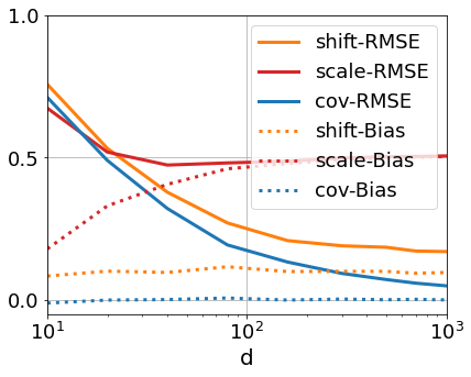
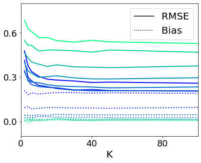
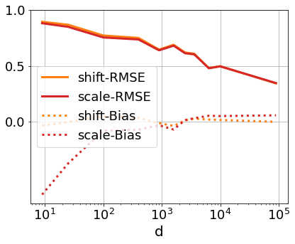
with and being a positive definite matrix. Obviously, is a convex function with respect to . As described in previous sections, given and a probability distribution on which satisfies , we estimate using samples from . The debiasing methods are tested for many different ’s and ’s. For each and , the experiment is repeated by times, and in each experiment we first sample a new set of noisy observations and then run the debiasing methods.
To measure and compare the performance of our debiasing methods, we compute the root mean squared error (RMSE) and the average bias of the estimates across experiments, and compare the values with that of the naive estimate. Concretely, let and be the estimate given by the debiasing method and the naive method in the -th experiment, respectively, we compute and compare the following two relative quantities:
| (28) |
By the definitions, when the debiasing method is effective, we expect and . The closer these quantities are to zero, the more effective the debiasing method. These two errors will also be studied in the experiments for other problems.
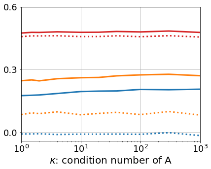
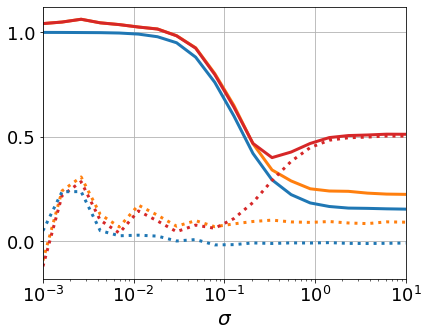
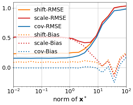
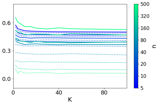
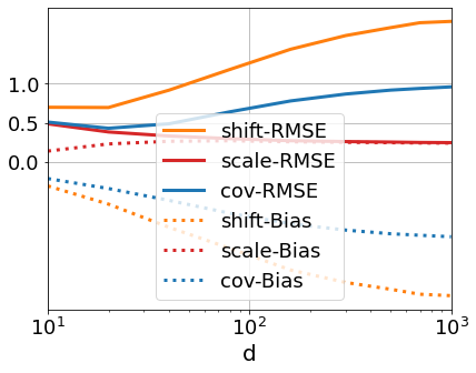
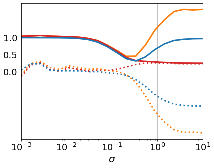
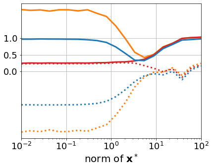
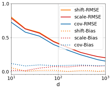
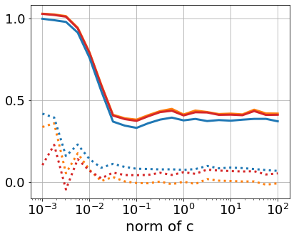
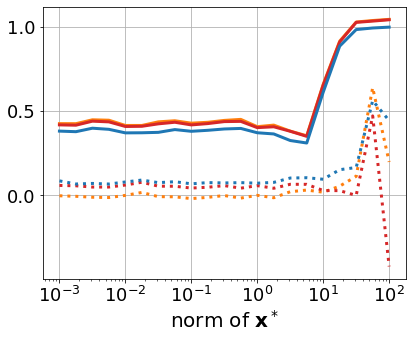
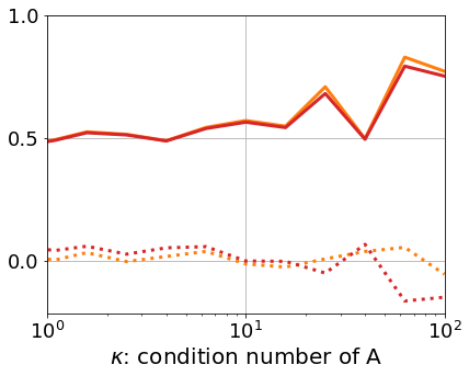
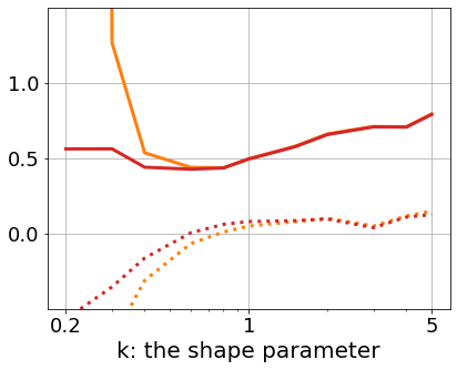
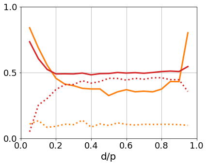
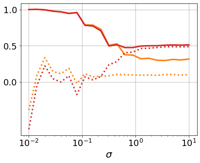
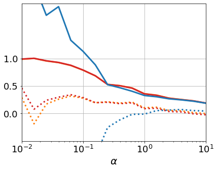
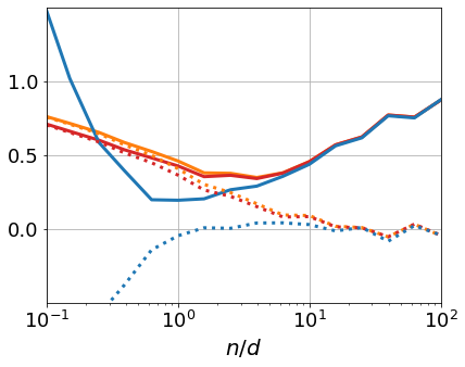
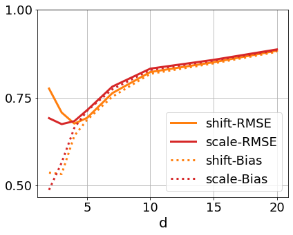
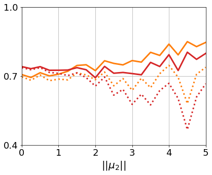
Before the debiasing methods are applied, a generic positive definite matrix is generated by its eigenvalue decomposition. Concretely, we generate a diagonal matrix with positive entries, and an orthogonal matrix , and then let . We take as an isotropic Gaussian distribution centered at , i.e. . The experiment results for (P1) are shown in Figure 1 and 2. In the experiments, we study the performance of all the three debiasing methods (shifting, scaling, covariance estimate) for problems with different dimensions (Figure 1 left), different condition numbers of (Figure 1 middle), different noisy strength (Figure 1 right), and different norm of (Figure 2 left). Throughout these experiments, we take noisy observations of , and do rounds of resampling when bootstrap is applied. The figures show that the shifting debiasing method and the covariance estimate method can usually significantly reduce the estimate error and bias, while the scaling method does not perform as well when the dimension is large or the noise is strong. The debiasing methods become less effective when the noise level is low or is large, in which case the noise observations are (effectively) close to and the naive estimate is already good. The experiments on the condition number of show that our methods are not sensitive to the spectrum of . Here we remark that the covariance estimate method performs especially well because the function is quadratic, hence the Hessian matrix has all information about the function.
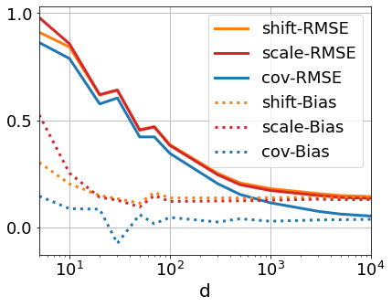
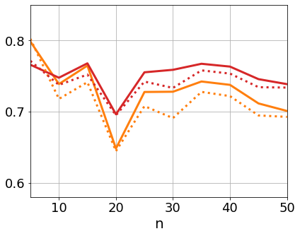
For the bootstrap methods, we also study the number of resampling rounds required for different . Results in Figure 2 show that a constant is usually sufficient to approach best-achievable performance for any . The RMSE almost stops decreasing after even when is much bigger. This shows that our theories in Section 3 can potentially be improved.
4.2 P2: Fourth-order polynomials
We then consider a higher-order polynomial function given by
| (P2) |
where and is a positive definite matrix. Compared with P1, this function has non-uniform curvature. It is flat when is small and grows fast when is large. In P2, we consider similar experiment settings as those for . We test the methods against problems with different dimensions, noise levels, and norms of . The results are shown in Figures 3. We see that for this problem only the scaling method performs well in most cases. The covariance estimate method works when and lie in specific ranges. The shifting method sometimes even performs worse than the naive estimate. Experiments on the condition number of still show that the methods are insensitive with . We ignore the figure here.
4.3 P3: Rational functions
Next, we consider a rational function
| (P3) |
where is the input and , are positive numbers. This function is convex for , . Hence, in the experiments, we take a coordinate-wise exponential distribution as . Fixing , we test our methods on problems with different dimensions, magnitudes of , and . Note that changing the magnitude of is equivalent with changing in the opposite direction. Results in Figure 4 show that the three debiasing methods perform similarly. They become more effective when the dimension of the problem increases. When is small or is large, the debiasing methods do not provide much improvement compared with the naive estimate. This is because in these cases the function is almost linear around and the convexity bias is small.
4.4 P4: Unconstrained optimization problems
When the objective function is parameterized by a parameter vector, the optimal value of some optimization problems is a convex or concave function of the parameters. For instance, let be the optimal value of the following minimization problem given some ,
| (29) |
where , are functions of . Then, is a concave function of because it is the minimum of a family of affine functions [3]. Therefore, our debiasing methods can be applied when we are interested in the minimum value of (29) at but can only get access to its noisy observations.
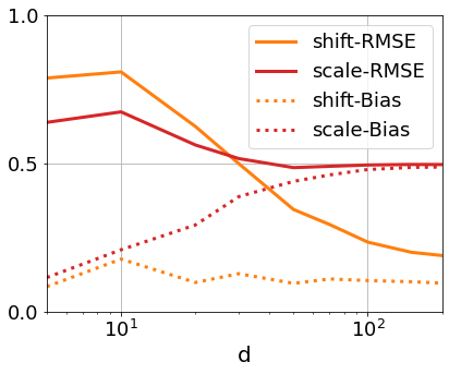
In the experiments, we consider specifically the minimization of a quadratic function when the Hessian of the objective function has some randomness, i.e. the concave function we debias is
| (P4) |
where is a positive definite matrix with randomness, and is a fixed vector. We easily have . Given a generic groundtruth Hessian matrix , where is the eigenvalue decomposition of and , we generate noisy observations of by sampling
where are independent random variables that follows the gamma distribution with shape and scale , whose density function is and expectation is . This makes sure that all noisy observations are positive definite.
Fixing and , Figure 5 shows the RMSEs and biases of the shifting and scaling methods for different dimensions, condition numbers of , and the shape parameter . Note that the actual dimension of the problem is . The results show that our methods are generally effective. The methods perform better when the dimension is higher, or the condition number of is not too large. When is small, i.e. the variance of the data distribution is large, the shifting method does not work well, while the scaling method keeps working well.
4.5 P5: Constrained optimization problem
Convex debiasing methods can also be applied to constrained optimization problems with randomness. The randomness can appear on the constraints. Consider
| (30) |
Fixing and , let be the optimal value of (30) given . Suppose strong duality holds, then
which shows that is the maximum of affine functions of . Therefore, is convex. The debiasing methods applies when we are interested in the optimal value at some while only its noisy observations can be obtained.
In the experiments, we estimate
| (P5) |
where , is a positive definite matrix, , and . Given , we take as an isotropic Gaussian distribution centered at , i.e. . Throughout the experiments, we fix and , and test the methods for different dimensions, ratio of , and noise level . Figure 6 shows the results. We see that both methods can significantly reduce the bias and RMSE, while the shifting method usually outperforms the scaling method. Better performance is achieved when is large, is not too close to , or is large.
4.6 P6: Entropy
Next, we test the estimate of entropy for discrete probability distributions, i.e.
| (P6) |
where satisfies and . We generate the groundtruth distribution from symmetric Dirichlet distribution with parameter . Noisy observations of are the empirical distributions of single samples from . In the experiments, we fix , and study the performance of the debiasing methods for problems with different dimension , , and the ratio of and .
For this problem, the covariance estimate method takes simple form. Let be the average of noisy observations of . Then, the covariance matrix is , and the Hessian of the entropy functional (viewed as a function of vector ) is . Hence, we have , and the debiased estimate is . It is the same as the classical debiasing scheme in [16].
The results are shown in Figure 7. For well-behaved problems, all three methods perform similarly. They can all significantly reduce the bias and error. When is small, i.e. the distribution is sparse, or when is small compared with , the bootstrap methods perform better than the covariance estimate method. We remark here that the experiments are part of the effort to show the wide applicability of our methods. Many delicate methods have been developed specifically for the entropy estimate problem, and we do not expect our methods to outperform all of them on this specific problem. Hence, we do not compare our methods with state-of-the-art methods here.
4.7 P7: Wasserstein distance
Finally, we estimate the 2-Wasserstein distance between a pair of distributions (, ) on , defined by
| (P7) |
where is a coupling of and whose two marginals are and , respectively. In the experiments, and are taken as Gaussian distributions and , where are two vectors fixed for all trials. Noisy observations of and are empirical distributions of i.i.d. samples of the distributions. The Wasserstein distance between empirical distributions are computed by a linear programming problem. Specifically, let be an empirical distribution on , be an empirical distribution on , is given by the following problem
| (31) |
where denotes the all-one vector with proper size.
In the experiments, without loss of generality, we take . We consider , and fix , . Figure 8 shows the results for problems with different dimension , , and . Results show that our methods can improve the naive estimate. The improvement gets smaller when the dimension is higher. This might be caused by the essential difficulty of estimating the Wasserstein distance in high dimensional spaces [22].
5 Summary
In this work, we propose a general framework to correct the bias introduced by convexity/concavity when estimating the value of functions or functionals. Our methods do not require domain knowledge of the objective functions, and can be applied as long as noisy observations of the groundtruth input are available. Numerical experiments on a wide range of problems show the effectiveness of our methods.
While our methods have general applicability, their performance may not be optimal on specific problems. For example, extensive researches are conducted on the estimate of entropy, and some proposed methods might have better empirical or theoretical properties than our methods. We emphasize that the value of our approach lies mostly on its generality—it can serve as an off-the-shelf tool to debias the estimate of convex functions and obtain improvement upon the naive estimate using the sample mean.
Nevertheless, the gain is not free—it comes with a price of additional computational cost. Compared with the naive estimate, our methods with bootstrap requires evaluating the function for multiple times. For some applications, such as optimization problems, evaluating the function can be expensive. Though, what to blame is not the methods, but the limited observations and knowledge on the problem. This is the cost of generality. If we have more domain knowledge, the covariance estimate method can be applied without high computational cost.
6 Proof of Theorem 2
6.1 Notations.
In the proof, we write if there exists a constant independent with such that always holds. When using these notations, the dimension is treated as a constant. We use to denote higher-order-terms appearing in the Taylor expansion. Specifically, for quantities and integer , denotes (sum of) terms with form with . When taking expectation, we use to denote the expectation over both the sampling of and the sampling of during bootstrap, and use to denote the expectation over the sampling of based on a fixed set of . The norm always means 2-norm. We use to denote the Hessian matrix of at , i.e. . For any matrix and vector , denote .
We use Einstein notations mostly when tensors with dimension are involved. When only vectors and matrices are involved, we still use the conventional matrix product notations. For vectors, we use superscript as the index of entries, and subscript as the index of the vector in a set of vectors. Entries are denoted by lower case letters. For example, the -th noisy observation vector is given by .
6.2 Main proof
To prove the theorem, first notice that
Hence, we only need to show . Let
Then, we have and , and
Note that and do not depend on the sampling of , by the law of total expectation, we have
and similarly . Therefore,
| (32) |
Next, we estimate the three terms on the right hand side of (32) separately. In the estimates below, we take terms as leading terms, and show that there is no term with lower order.
6.2.1 Estimate of .
In the proof, we will extensively use the Taylor expansion of and its derivatives. The results are given in Lemma 1. By the the Taylor expansion (59) in Lemma 1, we have
Taking expectation over , note that , we have
According to Lemma 2 and 3, we have
By the Taylor expansion (61) for , for any vector , we have
Therefore, for we have
Let
Then, we have
| (33) |
Taking square and expectation for (33), there exists a constant such that
| (34) |
Next, we give estimates to the terms in (34). We will use results in Lemma 6. First, Letting be the eigenvalue of with largest absolute value, we have
Therefore,
| (35) |
Next, for , we have
| (36) |
where the fourth to the fifth line is given by Lemma 6. Similarly, we can obtain . And by Lemma 7 and similar derivations, we can obtain . For , the Taylor expansion 62 gives
Taking square and by Lemma 6 we have . Therefore, considering , back to (34) we have
| (37) |
Next, by we obtain
Note that the terms with powers of become small quantities (no bigger than ) after taking expectation, we have
Thus,
Further notice that
Finally, since , we have the following estimate for :
| (38) |
6.2.2 Estimate of .
6.2.3 Estimate of
Taking Taylor expansion for , we have
| (42) |
We will estimate the three terms above using the estimate (33) for .
For the first term on the right hand side of (42), there exists a constant , such that
| (43) |
We first consider the first term on the right hand side of (43). For convenience, let , and . Then, we have , and
For the right hand side, we have
| (44) |
For the first term above, because of the independence of and , we have
| (45) |
For the second term in (44), by Lemma 6 we have
| (46) |
| (47) |
Next, we consider the second term on the right hand side of (43). Using the same notations as above, we have
For the right hand side, we have
| (48) |
By the independence of and , we obtain
| (49) |
Therefore, we have
| (50) |
For the third term in (43), recall that , , and , by Hölder’s inequality we have
| (51) |
For the second term on the right hand side of (42), there exists a constant , such that
| (53) |
where the estimate of follows similarly the estimate of
when we deal with .
For the first term on the right hand side of (53), we have
Note that from the fourth to the fifth line we are moving terms with into the term, and adding terms, which are also no bigger than . Hence, back to (53) we have
| (54) |
For the third term on the right hand side of (42), recall that , we have
| (55) |
6.2.4 Putting together.
6.3 Lemmas
In this section we provide and prove several lemmas used in the proof above. These lemmas may also be used in the proof of Theorem 3.
The first lemma gives Taylor expansions for and its derivatives based on Assumption 2. The results are standard in calculus, hence we ignore the proof.
Lemma 1.
Let be a function satisfying Assumption 2. Then, for any , we have the following Taylor expansions for and its derivatives:
| (59) | ||||
| (60) | ||||
| (61) | ||||
| (62) |
The next two lemmas deal with the expectation of quadratic forms and third order monomials over the choice of .
Lemma 2.
Let be the uniform distribution on points , and . Let be the empirical mean of samples i.i.d. sampled from , i.e. , . Let be an arbitrary matrix. Then,
Proof.
We ignore the subscript in the expectation. Obviously, we have and . Hence,
∎
Lemma 3.
Let be the uniform distribution on points , and . Let be the empirical mean of samples i.i.d. sampled by , i.e. , . Let be an arbitrary tensor. Then,
Proof.
The next lemma deals with the residual term of .
Lemma 4.
Let be the uniform distribution on points , and . Let be the empirical mean of samples i.i.d. sampled by , i.e. , . Then,
Proof.
The next two lemmas estimates the moments of , and . The first one is a general result for moments of the average of i.i.d random variables.
Lemma 5.
Let be a random variable taking values on , and are i.i.d copies of . Let . Let be a positive integer. Assume , and has up to -th order finite moments. Then, for any , we have .
Proof.
We first show the results for even . Consider the set
Let be the number of elements in . Then, is a number that depends only on . When is an even number, we have
| (66) |
The right hand side of (66) is the multinomial expansion of , organized according to the powers of different ’s in each term, and are positive integers related with multinomial coefficients. depends on and , but is independent with . Since , the expectation of is nonzero only when there is no that equals to . Hence, (66) equals to
| (67) |
Because are independent, we have . By the finite moment assumption of , we can find a constant such that holds for any . Then, we have
Moreover, since , we have , and hence
This completes the proof for even .
For odd , note that . The result follows by a Cauchy-Schwartz inequality:
∎
Lemma 6.
Let be a probability distribution on that satisfies Assumption 1, and be i.i.d samples from . Let , and . Then, for any positive integer , we have
Proof.
Finally, we study using similar approaches.
Lemma 7.
Let be a probability distribution on that satisfies Assumption 1, and is the uniform ditribution on . Consider i.i.d sampled from , and i.i.d sampled from . Let , and . Then, for any positive integer , we have
where the expectation is taken on both and .
Proof.
Following the proof of Lemma 5, fixing , for even number we have
| (68) |
When we consider the sampling of , we need to take an expectation of (68) over . For each term in the sums in (68), we have
where the first to the second line is given by the Hölder’s inequality, and the second to the third line is given by Lemma 6. Substituting the estimate above to (63), we have that there exists a constant independent with , such that
For odd we can show the result similar to the proof of Lemma 5 using the Cauchy-Schwartz inequality. ∎
7 Proof of Theorem 3
7.1 Additional notations
In this section, we will expand our use of the hot notations. We use to denote higher-order-terms with coefficients depending on or derivatives of evaluated at . For example,
can be represented by . By Lemma 1, , , and can be represented by . (Note that in the Taylor expansion the coefficients depends on , which is treated as a constant.) Hence, any can be represented by . Moreover, we use to denote higher-order-terms that expectations with respect to are taken for some parts. For example,
can be represented by . Using the Hölder’s inequality and Jensen’s inequality, it is easy to show that the does not change the order of the expectation of the higher-order-terms. For any , we have
7.2 Main proof
We take a similar path as the proof of Theorem 2. Specifically, in this section we consider another defined as , then we have
which gives the same form as the shifting debiasing, but with a different debiasing quantity. To prove the theorem, we still show .
We first decompose to separate the effect of the sampling of and the sampling of . Recall that
Define , , and
| (69) |
Then, we have
Denote
Then, we can write . Since , we know , and hence
| (70) |
Next, we estimate the terms in (70).
7.2.1 Estimate of
By Assumption 4, has a positive lower bound . Hence, we have and
Substituting the lower bounds into , we have
Therefore, by the Hölder’s inequality and the Jensen’s inequality,
For the , terms, by Lemma 10, we have
For the , , , and terms, by Lemma 11, they are all . Therefore, we have the following estimate for :
| (71) |
7.2.2 Estimate of
7.2.3 Estimate of
7.2.4 Estimate of
Note that
We first simplify the problem by noticing that and are both close to . Specifically, let
Then,
| (74) |
By the lower bound of and the Hölder’s inequality, we have
| (75) |
For the term in (75) with and , note that this term contains fourth-order monomials of and . Similar to the analysis in Section 7.2.1, we know this term has order . For the other term, by Jensen’s inequality we have
For the term on the last line, a Taylor expansion at gives
Therefore, we have
and back to (75) we have , and hence
Next, we study . By the definition of and , using the theorem of total expectation, we have
| (76) |
Taylor expansion of at gives
Here, the higher-order-terms notation means these terms depends on the derivatives of at . We note that a Taylor expansion of these derivatives at will replace the dependency on , and by powers of . It will not lower the order of the terms, Hence, the higher-order-terms can be written as . Plugging the Taylor expansions into (76), since , we obtain
| (77) |
where denotes higher-order-terms in which expectations over are taken for some terms. Similarly, we have
| (78) |
Combining (77) and (78), (76) becomes
| (79) |
Expanding and at , similar to arguments above Equation (77), we have
Moreover, by the analysis (40) in Section 6.2.2, we have
Back to (76), we have
Hence, for , we have
and for we have the same estimate
| (80) |
7.2.5 Estimate of
To estimate , we first study . Recall that
To simplify notations, we use , , to represent , , and when no confusion is caused. Our intuition is that is close to and is close to . Hence, we will try to expand and at . First, applying the identity for , we have
| (81) |
We will estimate the three terms in (81). We start from the first and the second terms.
For the first term , expanding at gives
| (82) |
For the second term in (81), we first expand and . For , similar to (82) we have
| (83) |
For , we have
| (84) |
We still replace by . Combining (83) and (84), we have
Therefore,
| (85) |
Combining (82) and (85), we have
Let . By Lemma 2 and 3, we have
| (86) |
Let
be the higher-order-terms in (86), and . Then, we have
Also let , then
| (87) |
Next, we come to estimate using the decomposition (87). Similar to (34), we have
| (88) |
Since is a fixed matrix, it is easy to show that
For , except the factors, it consists the sum of terms. All terms and their products are after taking expectation. (This can be shown rigorously by taking Taylor expansions of , , and at and applying Lemma 8 and 9.) Therefore, . For the higher-order-terms , by Lemma 8 and 9, we easily have .
For , by the lower bound of , we have
By Lemma 11, . By (84), the leading term of is a second-order term. Hence, the leading term of has order , which gives . Totally, we have . For , by a Taylor expansion of at , we have
| (89) |
Note that the leading term of is the term, which gives
Hence,
Finally, back to (88), we have
| (90) |
7.2.6 Estimate of
7.2.7 Estimate of
We take the same technique as in the proof of Theorem 2. Specifically, a Taylor expansion of at gives
| (92) |
Recall that when estimating we have the decomposition (87) :
and , , , , we have
| (93) |
and
| (94) |
Substituting (93) and (94) into (92), we have
| (95) |
For the first and the third terms in (95), note that and are fixed matrices. Following the proof in Section 6.2.3, we have
| (96) |
and
| (97) |
For the second term in (95), we define a tensor as
Then, by the Taylor expansion for (89), we have
Therefore, can be written as
and we have
| (98) |
Note that is a fixed tensor. Repeating the analysis that gives (50) with replacing , we have
| (99) |
7.2.8 Putting together
7.3 Lemmas
In this subsection we provide lemmas used in the proof of Theorem 3. Note that we will also make use of the lemmas in Section 6.
The first two lemmas are counterparts of Lemma 6 and 7 under the new assumption 3. The proof is similar to the proof of those Lemmas.
Lemma 8.
Let be a probability distribution on that satisfies Assumption 3, and are i.i.d sampled from . Let , and . Then, for any positive integer , we have
Lemma 9.
Let be a probability distribution on that satisfies Assumption 3, and is the uniform ditribution on . Consider i.i.d sampled from , and i.i.d sampled from . Let , and . Then, for any positive integer , we have
where the expectation is taken on both and .
The next two lemmas characterize the moments of , , and , . The and are defined in (69).
Lemma 10.
Under the same assumptions in Theorem 3, for any positive integer , we have
Proof.
First, we consider . Without loss of generality, assume is an even number. By the law of total expectation, we have
| (103) |
For , let , and be an i.i.d. copy of . Then, . Since are finite, we have . Let and . Then, by the Hölder’s inequality, for any , we have . Therefore, applying Lemma 5, we have
which implies
Back to (103), we have
| (104) |
Lemma 11.
Under the assumptions of Theorem 3, for any positive integer , we have
References
- [1] Jayadev Acharya, Alon Orlitsky, Ananda Theertha Suresh, and Himanshu Tyagi. Estimating rényi entropy of discrete distributions. IEEE Transactions on Information Theory, 63(1):38–56, 2016.
- [2] András Antos and Ioannis Kontoyiannis. Convergence properties of functional estimates for discrete distributions. Random Structures & Algorithms, 19(3-4):163–193, 2001.
- [3] Stephen Boyd, Stephen P Boyd, and Lieven Vandenberghe. Convex optimization. Cambridge university press, 2004.
- [4] Yuheng Bu, Shaofeng Zou, Yingbin Liang, and Venugopal V Veeravalli. Estimation of kl divergence: Optimal minimax rate. IEEE Transactions on Information Theory, 64(4):2648–2674, 2018.
- [5] Bradley Efron. Bootstrap methods: another look at the jackknife. In Breakthroughs in statistics, pages 569–593. Springer, 1992.
- [6] Philip Etter and Lexing Ying. Operator shifting for general noisy matrix systems. arXiv e-prints, pages arXiv–2104, 2021.
- [7] Philip A Etter and Lexing Ying. Operator shifting for noisy elliptic systems. arXiv preprint arXiv:2010.09656, 2020.
- [8] Shuyang Gao, Greg Ver Steeg, and Aram Galstyan. Efficient estimation of mutual information for strongly dependent variables. In Artificial intelligence and statistics, pages 277–286. PMLR, 2015.
- [9] Peter Grassberger. Entropy estimates from insufficient samplings. arXiv preprint physics/0307138, 2003.
- [10] Yanjun Han, Jiantao Jiao, and Tsachy Weissman. Minimax estimation of divergences between discrete distributions. IEEE Journal on Selected Areas in Information Theory, 1(3):814–823, 2020.
- [11] Yanjun Han, Jiantao Jiao, Tsachy Weissman, and Yihong Wu. Optimal rates of entropy estimation over lipschitz balls. The Annals of Statistics, 48(6):3228–3250, 2020.
- [12] William James and Charles Stein. Estimation with quadratic loss. In Breakthroughs in statistics, pages 443–460. Springer, 1992.
- [13] Jiantao Jiao, Kartik Venkat, Yanjun Han, and Tsachy Weissman. Minimax estimation of functionals of discrete distributions. IEEE Transactions on Information Theory, 61(5):2835–2885, 2015.
- [14] Alexander Kraskov, Harald Stögbauer, and Peter Grassberger. Estimating mutual information. Physical review E, 69(6):066138, 2004.
- [15] Tomáš Marek, P Tichavsky, G Dohnal, et al. On the estimation of mutual information. J. A, Dohnal G, editors, 2008.
- [16] George Miller. Note on the bias of information estimates. Information theory in psychology: Problems and methods, 1955.
- [17] Liam Paninski. Estimation of entropy and mutual information. Neural computation, 15(6):1191–1253, 2003.
- [18] Charles Stein. Variate normal distribution. In Proceedings of the Third Berkeley Symposium on Mathematical Statistics and Probability: Contributions to the Theory of Statistics, volume 1, page 197. University of California Press, 1956.
- [19] Paul Valiant and Gregory Valiant. Estimating the unseen: improved estimators for entropy and other properties. Advances in Neural Information Processing Systems, 26, 2013.
- [20] Sergio Verdú. Empirical estimation of information measures: A literature guide. Entropy, 21(8):720, 2019.
- [21] Vincent Q Vu, Bin Yu, and Robert E Kass. Coverage-adjusted entropy estimation. Statistics in medicine, 26(21):4039–4060, 2007.
- [22] Jonathan Weed and Francis Bach. Sharp asymptotic and finite-sample rates of convergence of empirical measures in wasserstein distance. Bernoulli, 25(4A):2620–2648, 2019.
- [23] David H Wolpert and David R Wolf. Estimating functions of probability distributions from a finite set of samples. Physical Review E, 52(6):6841, 1995.
- [24] Yihong Wu and Pengkun Yang. Minimax rates of entropy estimation on large alphabets via best polynomial approximation. IEEE Transactions on Information Theory, 62(6):3702–3720, 2016.
- [25] Samuel Zahl. Jackknifing an index of diversity. Ecology, 58(4):907–913, 1977.