Private Estimation with Public Data

Abstract

We initiate the study of differentially private (DP) estimation with access to a small amount of public data. For private estimation of $d$-dimensional Gaussians, we assume that the public data comes from a Gaussian that may have vanishing similarity in total variation distance with the underlying Gaussian of the private data. We show that under the constraints of pure or concentrated DP, $d+1$ public data samples are sufficient to remove any dependence on the range parameters of the private data distribution from the private sample complexity, which is known to be otherwise necessary without public data. For separated Gaussian mixtures, we assume that the underlying public and private distributions are the same, and we consider two settings: (1) when given a dimension-independent amount of public data, the private sample complexity can be improved polynomially in terms of the number of mixture components, and any dependence on the range parameters of the distribution can be removed in the approximate DP case; (2) when given an amount of public data linear in the dimension, the private sample complexity can be made independent of range parameters even under concentrated DP, and additional improvements can be made to the overall sample complexity.

1 Introduction

Differential privacy (DP) [DMNS06] guarantees the privacy of every point in a dataset. This is a strong requirement, and often gives rise to qualitatively new requirements when performing private data analysis. For instance, for the problem of private mean estimation (under pure or concentrated DP), the analyst must specify a guess for the unknown parameter, and needs more data to get an accurate estimate depending on how good their guess is. This cost can be prohibitive in cases where the data domain may be unfamiliar.

Fortunately, in many cases, it is natural to assume that there exists an additional public dataset. This public dataset may vary in both size and quality. For example, one could imagine that a fraction of users opt out of privacy considerations, giving a small set of public in-distribution data. Alternatively, it is common to pretrain models on large amounts of public data from the web, which may be orders of magnitude larger than the private data but significantly out of distribution. In a variety of such settings, this public data can yield dramatic theoretical and empirical improvements to utility in private data analysis (see discussion in Section 1.3). We seek to answer the following question:

How can one take advantage of public data for private estimation?

We initiate the study of differentially private statistical estimation with a supplementary public dataset. In particular, our goal is to understand when a small amount of public data can significantly reduce the cost of private estimation.

1.1 Results

We investigate private estimation with public data through the canonical problems of learning Gaussians and mixtures of Gaussians.

Gaussians.

In the case of pure and concentrated differential privacy, exactly $d+1$ public points are sufficient to remove any dependence on “range parameters” in the private sample complexity, even when the underlying Gaussian distribution of the public data bears almost no similarity to that of the private data. We start with following result for the scenario when the two distributions are the same.

Theorem 1.1.

For all $\alpha,\beta,\varepsilon>0$ and $d\geq 1$ there exists a computationally efficient $\frac{\varepsilon^{2}}{2}$-zCDP (and a computationally inefficient $(\varepsilon,0)$-DP) algorithm $\mathcal{M}$ that takes $n$ private samples and $d+1$ public samples from a $d$-dimensional Gaussian $D$, and is private with respect to the private samples, such that if

$$n=O\mathopen{}\mathclose{{}\left(\frac{d^{2}}{\alpha^{2}}+\frac{d^{2}}{\alpha\varepsilon}}\right)\cdot\mathrm{polylog}\mathopen{}\mathclose{{}\left(d,\frac{1}{\beta},\frac{1}{\alpha}}\right),$$

then $\mathcal{M}$ estimates the parameters of $D$ to within total variation error $\alpha$ with probability at least $1-\beta$.

Without public data, the analyst would be required to specify a bound $R$ on the $\ell_{2}$ norm of the mean and a bound $K$ on the condition number of the covariance, and the private sample complexity would scale logarithmically in terms of these parameters (which we denote as range parameters). Thus, this cost could be arbitrarily large, or even infinite, given poor a priori knowledge of the problem. Note that these requirements are not due to suboptimality of current private algorithms. Packing lower bounds for estimation under pure and concentrated DP show that dependence on range parameters is an inherent cost of privacy. However, this dependence can be entirely eliminated at the price of $d+1$ public data points, which is less public data than the non-private $\Theta(\tfrac{d^{2}}{\alpha^{2}})$ sample complexity of the problem. For estimating Gaussians with identity or known covariance (that is, mean estimation) it turns out that just one public sample suffices to remove all dependence on range parameters.

The next natural question to ask is: what if our public data does not come from the same distribution as our private data? Indeed, in practical settings, there may be significant domain shift between data that is publicly available and the private data of interest. Our next result shows that we can relax this assumption: it suffices that our public data comes from another Gaussian that is at most $\gamma<1$ away in total variation distance from the underlying private data distribution.

Theorem 1.2.

For all $\alpha,\beta,\varepsilon>0$, $d\geq 1$, and $0\leq\gamma<1$, there exists a computationally efficient $\frac{\varepsilon^{2}}{2}$-zCDP (and a computationally inefficient $(\varepsilon,0)$-DP) algorithm $\mathcal{M}$ that takes $n$ private samples from a $d$-dimensional Gaussian $D$, and $d+1$ public samples from a $d$-dimensional Gaussian $\widetilde{D}$ with $\mathrm{d_{TV}}(D,\widetilde{D})\leq\gamma$, and is private with respect to the private samples, such that if

$$n=O\mathopen{}\mathclose{{}\left(\frac{d^{2}}{\alpha^{2}}+\frac{d^{2}}{\alpha\varepsilon}}\right)\cdot\mathrm{polylog}\mathopen{}\mathclose{{}\left(d,\frac{1}{\beta},\frac{1}{\alpha},\frac{1}{1-\gamma}}\right),$$

then $\mathcal{M}$ estimates the parameters of $D$ to within total variation error $\alpha$ with probability at least $1-\beta$.

The upper bound on the total variation gap $\gamma$ results in the sample complexity picking up an extra $\mathrm{polylog}(\tfrac{1}{1-\gamma})$ factor. For instance, even when the public and private distributions have total variation distance $1-1/d^{100}$ (that is, they are almost entirely dissimilar), we incur only an extra $\mathrm{polylog}(d)$ factor in the sample complexity. In particular, note that the public dataset may be simultaneously quite small and significantly out of distribution with respect to the private data.

Mixtures of Gaussians.

We focus on estimation of mixtures of $k$ separated Gaussians in $d$ dimensions. Specifically, we assume that, given mixture components $\mathcal{N}(\mu_{i},\Sigma_{i})$ with respective mixing weights $w_{i}$ for $i\in[k]$ (with $w_{i}\geq w_{\min}$), then for each $i\neq j$,

$$\mathopen{}\mathclose{{}\left\lVert\mu_{i}-\mu_{j}}\right\rVert_{2}\geq\widetilde{\Omega}\mathopen{}\mathclose{{}\left(\sqrt{k}+\frac{1}{\sqrt{w_{i}}}+\frac{1}{\sqrt{w_{j}}}}\right)\cdot\max\mathopen{}\mathclose{{}\left\{\sqrt{\|\Sigma_{i}\|_{2}},\sqrt{\|\Sigma_{j}\|_{2}}}\right\}.$$ (1)

Private estimation of such mixtures of Gaussians (without public data) was previously studied by [KSSU19]. Their algorithms proceed in two stages: first, a clustering step to isolate the samples from each component, and an estimation step, which estimates the parameters of each individual Gaussian using the isolated samples from each component. Our algorithms follow a similar structure, but employ the public data at appropriate points in the procedure to enable substantial savings.

We provide two flavours of results for learning mixtures of Gaussians. First, we investigate the setting when we have a very small, dimension-independent amount of public data.

Theorem 1.3.

For all $\alpha,\beta,\varepsilon,\delta>0$, there exists an $(\varepsilon,\delta)$-DP algorithm $\mathcal{M}$ that takes $n$ private samples and $m$ public samples from a Gaussian mixture $D$ satisfying (1), such that if

$$n=O\mathopen{}\mathclose{{}\left(\frac{d^{2}}{w_{\min}\alpha^{2}}+\frac{d^{2}}{w_{\min}\alpha\varepsilon}+\frac{d^{1.5}k^{2.5}}{\varepsilon}}\right)\cdot\mathrm{polylog}\mathopen{}\mathclose{{}\left(d,k,\frac{1}{\beta},\frac{1}{\alpha},\frac{1}{\varepsilon},\frac{1}{\delta}}\right)~{}~{}~{}\text{and}~{}~{}~{}m=O\mathopen{}\mathclose{{}\left(\frac{\log(k/\beta)}{w_{\min}}}\right),$$

then $\mathcal{M}$ estimates the parameters of $D$ to within total variation error $\alpha$ with probability at least $1-\beta$.

Theorem 1.4.

For all $\alpha,\beta,\rho>0$, there exists an $\rho$-zCDP algorithm $\mathcal{M}$ that takes $n$ private samples and $m$ public samples from a Gaussian mixture $D$ satisfying (1), such that if for each $i\in[k]$, $\|\mu_{i}\|_{2}\leq R$ and $\mathbb{I}\preceq\Sigma_{i}\preceq K\mathbb{I}$, and

$$n=O\mathopen{}\mathclose{{}\left(\frac{d^{2}}{w_{\min}\alpha^{2}}+\frac{d^{2}}{w_{\min}\alpha\sqrt{\rho}}+\frac{d^{1.5}k^{2.5}}{\sqrt{\rho}}}\right)\cdot\mathrm{polylog}\mathopen{}\mathclose{{}\left(d,k,K,R,\frac{1}{\beta},\frac{1}{\alpha},\frac{1}{\rho}}\right)~{}~{}~{}\text{and}~{}~{}~{}m=O\mathopen{}\mathclose{{}\left(\frac{\log(k/\beta)}{w_{\min}}}\right),$$

then $\mathcal{M}$ estimates the parameters of $D$ to within total variation error $\alpha$ with probability at least $1-\beta$.

Our results differ from the prior work of [KSSU19] in the following ways: (1) we have results for both approximate DP and zCDP, as opposed to just approximate DP in [KSSU19]; (2) the private sample complexity due to the clustering step does not involve any dependence on the range parameters; and (3) the sample complexity due to the clustering step is now $O(d^{1.5}k^{2.5})$, as opposed to $O(d^{1.5}k^{9.06})$, which is a significant improvement, and shows up only due to applications of private PCA under better sensitivity guarantees. As far as the private sample complexity in the component estimation process is concerned, in the case of approximate DP, we have expressions independent of distribution parameters owing to the recent Gaussian learner by [AL21].

Finally, we investigate Gaussian mixture estimation with an amount of public data which is linear in the dimension.

Theorem 1.5.

For all $\alpha,\beta,\varepsilon,\delta>0$, there exists an $(\varepsilon,\delta)$-DP algorithm $\mathcal{M}$ that takes $n$ private samples and $m$ public samples from a Gaussian mixture $D$ satisfying (1), such that if

$$n=O\mathopen{}\mathclose{{}\left(\frac{d^{2}}{w_{\min}\alpha^{2}}+\frac{d^{2}}{w_{\min}\alpha\varepsilon}}\right)\cdot\mathrm{polylog}\mathopen{}\mathclose{{}\left(d,k,\frac{1}{\beta},\frac{1}{\alpha},\frac{1}{\varepsilon},\frac{1}{\delta}}\right)~{}~{}~{}\text{and}~{}~{}~{}m=O\mathopen{}\mathclose{{}\left(\frac{d\log(k/\beta)}{w_{\min}}}\right),$$

then $\mathcal{M}$ estimates the parameters of $D$ to within total variation error $\alpha$ with probability at least $1-\beta$.

Theorem 1.6.

For all $\alpha,\beta,\rho>0$, there exists an $\rho$-zCDP algorithm $\mathcal{M}$ that takes $n$ private samples and $m$ public samples from a Gaussian mixture $D$ satisfying (1), such that if

$$n=O\mathopen{}\mathclose{{}\left(\frac{d^{2}}{w_{\min}\alpha^{2}}+\frac{d^{2}}{w_{\min}\alpha\sqrt{\rho}}}\right)\cdot\mathrm{polylog}\mathopen{}\mathclose{{}\left(d,k,\frac{1}{\beta},\frac{1}{\alpha},\frac{1}{\rho}}\right)~{}~{}~{}\text{and}~{}~{}~{}m=O\mathopen{}\mathclose{{}\left(\frac{d\log(k/\beta)}{w_{\min}}}\right),$$

then $\mathcal{M}$ estimates the parameters of $D$ to within total variation error $\alpha$ with probability at least $1-\beta$.

Using $\widetilde{O}(d/w_{\min})$ public samples establishes all the advantages that using $\widetilde{O}(1/w_{\min})$ public samples gives, but additionally improves the private sample complexity even further. As we will describe in the technical overview, the clustering process is done entirely using the public data, and ends up removing the term due to private PCA from the private sample complexity in both approximate DP and zCDP regimes. Additionally, in the zCDP case, we do not have any dependence on distribution range parameters even in the component estimation process because we can use results from Theorem 1.1 this time.

1.2 Technical Overview

1.2.1 Estimating Gaussians

To start, we make the simple observation that for identity covariance Gaussians $\mathcal{N}(\mu,\mathbb{I})$, a single public sample is sufficient to remove the a priori assumption that $\|\mu\|_{2}\leq R$, which is required to obtain a finite sample complexity under pure and concentrated DP. Given a single public sample $\widetilde{X}$, Gaussian concentration implies that with probability at least $1-\beta$, the true mean lies within $\widetilde{O}(\sqrt{d})$ of $\widetilde{X}$. Hence, setting $R=\widetilde{O}(\sqrt{d})$ and starting with our coarse estimate $\widetilde{X}$, we can directly apply the $\tfrac{\varepsilon^{2}}{2}$-zCDP “clip-and-noise” Gaussian mechanism to get a sample complexity of $\widetilde{O}(\tfrac{d}{\alpha^{2}}+\tfrac{d}{\varepsilon\alpha})$, or the efficient $\varepsilon$-DP algorithm from [HKM22] to arrive at a $\widetilde{O}(\tfrac{d}{\alpha^{2}\varepsilon})$ sample complexity with no dependence on $R$ in either case.

We apply the same strategy to estimate the parameters of a general $d$-dimensional Gaussian. First, we compute the sample mean and covariance of $d+1$ public samples. Then we shift our private samples with respect to the public sample mean, and then rescale them according to the public sample covariance. The distribution of the resulting transformed private samples satisfy, with probability at least $1-\beta$ over public samples, $\mathrm{poly}(d,\tfrac{1}{\beta})$ range bounds on both the norm of the mean and the condition number of the covariance. This means we can apply either the concentrated DP Gaussian learner from [KLSU19] or the pure DP Gaussian learner from [BKSW19] (followed by inverting the shift and scale) to arrive at a successful learner matching the private sample complexity up to logarithmic factors of these learners that require these a priori range bounds, but now without any dependence on them.

Finally, we extend our results to the case where the public data comes from a Gaussian that is at most $\gamma$ far in TV distance from the private data distribution. We translate the $\gamma$-TV bound on the public and the private data distributions to a bound on the differences in their parameters. Taking this into account when applying our shift and rescaling with the public data yields $\mathrm{poly}(d,\tfrac{1}{\beta},\tfrac{1}{1-\gamma})$ range bounds on the transformed private data distribution’s parameters, which suffices to apply the same private learners as described earlier.

1.2.2 Estimating Gaussian Mixtures

The general process of estimating the parameters of Gaussian mixtures involves separating the mixture components by using techniques like PCA, followed by their isolation, and finally by individual component estimation. In other words, the components are first projected onto a low-dimensional subspace of $\mathbb{R}^{d}$, which separates the large mixture components from the rest, given that the separation in the original space is enough. The subspace is computed with respect to the available data, that is, it is chosen to be the top $k$ subspace of the data matrix, which preserves the original distances between the individual components, but shrinks down each component so that the intra-component distances are small but inter-component distances are large still. This allows us to separate a group of components from the rest. Repeating this process on each group, we can narrow down to a single Gaussian in each group, and estimate its parameters.

This has been the high-level idea in a lot of prior work, both non-private [VW02, AM05] and private [KSSU19]. In our setting, we utilise the public data available in different settings at various points to establish these tasks, while having a low cost in the sample complexity of the private data. Given a lower bound on the mixing weights ($w_{\min}$), we consider two settings in terms of the availability of the public data: (1) when there is very little available – $\widetilde{O}(1/w_{\min})$; and (2) when there is a lot more available – $\widetilde{O}(d/w_{\min})$. The key challenge, as indicated, is accurate clustering of data.

Public Data Sample Complexity: $\widetilde{O}(1/w_{\min})$

Clustering.

This is the more challenging setting of the two because there is not enough public data for techniques such as PCA to give accurate results. We therefore have to rely on the private data for these tasks, and use their private counterparts to get the desired results.

1. Superclustering to reduce sensitivity for Private PCA: The main goal, as in most private estimation tasks, is to reduce the amount of noise added for privacy in order to get better accuracy. This boils down to limiting the sensitivity of the target empirical function of the data. For this, we would like to make sure that the range of the data (to which, we scale the noise) is very tight – in our context, it means that we would like to have a ball that contains a group of mixture components, which are very close to one another, having close to the smallest possible radius. We can limit the data to within this ball, and the sensitivity for the next step would be reduced. To get such a ball, we use the public data, and come up with a “superclustering” algorithm, which does exactly that. This algorithm essentially relies on the concentration properties of high-dimensional Gaussians – it finds the radius of the largest Gaussian and a point (as the centre) within that Gaussian, and additively grows the ball until it stops finding more points. This gives a ball whose radius is an $O(k)$ approximation to the radius of the largest Gaussian. We use this ball to isolate the same components in the private data, and perform private PCA to separate the components within. Getting this tight ball is crucial to reduce the cost of private PCA in terms of the sample complexity compared to the prior work of [KSSU19].

2. Private PCA: We use the well-known private PCA algorithm that has been previously analysed in [DTTZ14, KSSU19] for this.

3. Partitioning in low dimensions: The next task is to partition the components in the low-dimensional subspace in a way that there is no overlap. For this, we use an algorithm that is similar to the “terrific ball” algorithm of [KSSU19], and relies upon the accuracy guarantees of the private PCA step. It uses both public and private data, and looks for a terrific ball within them. If there is one, indicating that there is more than one component in that subset of the datasets, it partitions the datasets (and the components), and queues the partitions for further work. Otherwise, it just adds that subset of the private dataset to the set of discovered clusters.

4. The whole process is repeated on all the remaining partitions.

Component Estimation.

The final task is to estimate the parameters of the $k$ isolated components. In the $(\varepsilon,\delta)$-DP setting, we simply apply the private Gaussian learner of [AL21] to each component, which enables us to learn with no dependence in the sample complexity on the range parameters of the Gaussian itself (among other available choices, were the $(\varepsilon,\delta)$-DP learners from [KMSSU21, KMV21, TCKMS21], but this one had the joint best sample complexity with [TCKMS21]). In the $\rho$-zCDP setting, we use the Gaussian learner from [KLSU19], instead. Note that in this setting, the private sample complexity does depend on the range parameters of the Gaussians, themselves.

Public Data Sample Complexity: $\widetilde{O}(d/w_{\min})$

Clustering.

In the second setting, clustering is easier in terms of the tasks that need to be done privately – it can be done entirely by using the public dataset itself. This time, the number of public samples is enough to be able to accurately do PCA on the public data, hence, perform clustering using just the public data itself. This improves the private data sample complexity by removing the term due to private PCA altogether.

1. No supercustering involved: The first change in the clustering algorithm is eliminating the superclustering step.

2. PCA: We essentially get the projection matrix for the top $k$ subspace of the data using non-private PCA, and work within that subspace using the public data to further partition the two datasets (and the components).

3. Partitioning in low dimensions: The algorithm for partitioning in the low-dimensional subspace is similar to the private partitioner used in the previous case, except that there is no need for privacy in this case.

4. The whole process is repeated on all the remaining partitions.

Component Estimation.

Once the components are separated, as before, we individually estimate them using the partitions of the private dataset privately. In the $(\varepsilon,\delta)$-DP setting, we again use the learner from [AL21], which ensures parameter-free private data sample complexity in this process. In the $\rho$-zCDP setting though, we use our own zCDP learner from this text (Theorem 1.1), which uses the public data, as well, to ensure parameter-free private data sample complexity for this process.

1.3 Related Work

A large part of our work focuses on using public data to remove the dependence on range parameters in private estimation. Understanding these dependences without public data has been a topic of significant study. [KV18] investigated private estimation of univariate Gaussians, showing that logarithmic dependences on the range parameters were both necessary and sufficient for pure differential privacy, but by using stability-based histograms [KKMN09, BNS16a], they could be removed under approximate differential privacy. Similar results have been shown in the multivariate setting: while logarithmic dependences are necessary and sufficient under pure or concentrated DP [KLSU19], they can be removed under approximate DP [AAK21, KMSSU21, TCKMS21, AL21, KMV21, LKO21]. More broadly, a common theme is that the dependences which are intrinsic to pure or concentrated DP can be eliminated by relaxing to approximate DP. Our results demonstrate that instead of relaxing the privacy definition for all the data, one can achieve the same goal by employing a much smaller amount of public data.

Our investigation fits more broadly into a line of work employing public data for private data analysis. Works, both theoretical and empirical, investigate the role of public data in private query release, synthetic data generation, and prediction [JE13, BNS16, ABM19, NB20, BCMNUW20, BMN20, LVSUW21]. For distribution-free classification with public and private data, it was shown in [ABM19] that, roughly speaking, if a hypothesis class is privately learnable with a small amount of public data ($o(1/\alpha)$), it is privately learnable with no public data. For density estimation, we show that the family of unbounded Gaussians is learnable with a small amount of public data ($\alpha$-independent), despite the fact that it is not learnable with only private data.

Additionally, a number of empirical works study the efficacy of public data in private machine learning, including methods such as public pre-training [ACGMMTZ16, PCSTE19, TB21, LWAFF21, YZCL21, LTLH22, Yu+22], using public data to compute useful statistics about the private gradients [ZWB21, YZCL21, KRRT21, AGMRSSSTT21], or using unlabeled public data to train a student model [PAEGT17, PSMRTE18, BTGT18].

Another setting with mixed privacy guarantees is when different users may require local versus central differential privacy [AKZHL17]. Mean estimation has also been studied in this setting [ADK19].

2 Preliminaries

2.1 Notation

We define some notation here to be used throughout the paper.

• Public data is denoted by $\widetilde{X}=(\widetilde{X}_{1},\dots,\widetilde{X}_{m})$, with each $\widetilde{X}_{i}\in\mathbb{R}^{d}$. Private data is denoted by $X=(X_{1},\dots,X_{n})$, with each $X_{j}\in\mathbb{R}^{d}$.

• We denote a ball of radius $r>0$ centred around a point $c\in\mathbb{R}^{d}$ by $B_{r}(c)$.

• For a set $S$, we denote its power set by $\mathcal{P}(S)$.

2.2 Useful Concentration Inequalities

We first state a multiplicative Chernoff bound.

Lemma 2.1 (Multiplicative Chernoff).

Let $X_{1},\dots,X_{m}$ be independent Bernoulli random variables, and let $X$ be their sum. If $p={\mathbb{E}\mathopen{}\mathclose{{}\left(X_{i}}\right)}$, then for $0\leq\delta_{1}\leq 1$ and $\delta_{2}\geq 0$,

$${\mathbb{P}\mathopen{}\mathclose{{}\left(X\leq(1-\delta_{1})pm}\right)}\leq e^{-\frac{\delta_{1}^{2}pm}{2}}$$

and

$${\mathbb{P}\mathopen{}\mathclose{{}\left(X\leq(1+\delta_{2})pm}\right)}\leq e^{-\frac{\delta_{2}^{2}pm}{2+\delta_{2}}}.$$

Next, we state Bernstein’s inequality.

Lemma 2.2 (Bernstein’s Inequality).

Let $X_{1},\dots,X_{m}$ be independent Bernoulli random variables. Let $p={\mathbb{E}\mathopen{}\mathclose{{}\left(X_{i}}\right)}$. Then for $m\geq\frac{5p}{2\varepsilon^{2}}\ln(2/\beta)$ and $\varepsilon\leq p/4$,

$${\mathbb{P}\mathopen{}\mathclose{{}\left(\mathopen{}\mathclose{{}\left|\frac{1}{m}\sum{X_{i}}-p}\right|\geq\varepsilon}\right)}\leq 2e^{-\varepsilon^{2}m/2(p+\varepsilon)}\leq\beta.$$

Now, we state the Hanson-Wright inequality about quadratic forms.

Lemma 2.3 (Hanson-Wright inequality [HW71]).

Let $X\sim\mathcal{N}(0,\mathbb{I}_{d\times d})$ and let $A$ be a $d\times d$ matrix. Then for all $t>0$, the following two bounds hold:

$${\mathbb{P}\mathopen{}\mathclose{{}\left(X^{T}AX-\mathrm{tr}(A)\geq 2\|A\|_{F}\sqrt{t}+2\|A\|_{2}t}\right)}\leq\exp(-t);$$

$${\mathbb{P}\mathopen{}\mathclose{{}\left(X^{T}AX-\mathrm{tr}(A)\leq-2\|A\|_{F}\sqrt{t}}\right)}\leq\exp(-t).$$

We mention an inequality that bounds the tails of a one-dimensional Gaussian $\mathcal{N}(\mu,\sigma^{2})$.

Lemma 2.4 ($1$-D Gaussian Concentration).

Let $Z\sim\mathcal{N}(\mu,\sigma^{2})$. Then,

$${\mathbb{P}\mathopen{}\mathclose{{}\left(|Z-\mu|\leq t\sigma}\right)}\leq 2e^{-\frac{t^{2}}{2}}.$$

Next, we state a concentration inequality for $0$-mean Laplace random variables.

Lemma 2.5 (Laplace Concentration).

Let $Z\sim\mathrm{Lap}(t)$. Then ${\mathbb{P}\mathopen{}\mathclose{{}\left(\mathopen{}\mathclose{{}\left|Z}\right|>t\cdot\ln(1/\beta)}\right)}\leq\beta.$

We now mention an anti-concentration inequality for weighted $\chi^{2}$ distributions from [ZZ18]. We adjust the constants appropriately in the following theorem as per the specifications in the aforementioned article.

Lemma 2.6 (Theorem 6 from [ZZ18]).

Let $Z\sim\mathcal{N}(0,1)$, $a>0$, and $Y=aZ$. Then for $\tau\geq a$, we have the following.

$${\mathbb{P}\mathopen{}\mathclose{{}\left(Y\geq a+\tau}\right)}\geq 0.06e^{-\frac{3\tau}{2a}}$$

The following are standard concentration results for the empirical mean and covariance of a set of Gaussian vectors (see, e.g., [DKKLMS16]).

Lemma 2.7.

Let $X_{1},\dots,X_{n}$ be i.i.d. samples from $\mathcal{N}(0,\mathbb{I}_{d\times d})$. Then we have that

$${\mathbb{P}\mathopen{}\mathclose{{}\left(\mathopen{}\mathclose{{}\left\|\frac{1}{n}\sum_{i\in[n]}X_{i}}\right\|_{2}\geq t}\right)}\leq 4\exp(c_{1}d-c_{2}nt^{2});$$

$${\mathbb{P}\mathopen{}\mathclose{{}\left(\mathopen{}\mathclose{{}\left\|\frac{1}{n}\sum_{i\in[n]}X_{i}X_{i}^{T}-I}\right\|_{2}\geq t}\right)}\leq 4\exp(c_{3}d-c_{4}n\min(t,t^{2})),$$

where $c_{1},c_{2},c_{3},c_{4}>0$ are some absolute constants.

2.3 Gaussian Mixtures

Here, we provide preliminaries for the problem of parameter estimation of mixtures of Gaussians. Let $\mathsf{Sym}_{d}^{+}$ denote set of all $d\times d$, symmetric, and positive semidefinite matrices. Let $\mathcal{G}(d)=\{\mathcal{N}(\mu,\Sigma):\mu\in\mathbb{R}^{d},\Sigma\in\mathsf{Sym}_{d}^{+}\}$ be the family of $d$-dimensional Gaussians. We can now define the class $\mathcal{G}(d,k)$ of mixtures of Gaussians as follows.

Definition 2.8 (Gaussian Mixtures).

The class of Gaussian $k$-mixtures in $\mathbb{R}^{d}$ is

$$\mathcal{G}(d,k)\coloneqq\mathopen{}\mathclose{{}\left\{\sum\limits_{i=1}^{k}{w_{i}G_{i}}:G_{1},\dots,G_{k}\in\mathcal{G}(d),w_{1},\dots,w_{k}>0,\sum_{i=1}^{k}w_{i}=1}\right\}.$$

We can specify a Gaussian mixture by a set of $k$ tuples as: $\{(\mu_{1},\Sigma_{1},w_{1}),\dots,(\mu_{k},\Sigma_{k},w_{k})\},$ where each tuple represents the mean, covariance matrix, and mixing weight of one of its components. Additionally, for each $i$, we refer to $\sigma_{i}^{2}=\mathopen{}\mathclose{{}\left\lVert\Sigma_{i}}\right\rVert_{2}$ as the maximum directional variance of component $i$.

We assume that the mixing weight of each component is lower bounded by $w_{\min}$. We impose a separation condition for mixtures of Gaussians to be able to learn them.

Definition 2.9 (Separated Mixtures).

For $s>0$, a Gaussian mixtures $\mathcal{D}\in\mathcal{G}(d,k)$ is $s$-separated if

$$\forall 1\leq i<j\leq k,~{}~{}~{}\mathopen{}\mathclose{{}\left\lVert\mu_{i}-\mu_{j}}\right\rVert_{2}\geq\mathopen{}\mathclose{{}\left(s+\frac{10}{\sqrt{w_{i}}}+\frac{10}{\sqrt{w_{j}}}}\right)\cdot\max\{\sigma_{i},\sigma_{j}\}.$$

We denote the family of separated Gaussian mixtures by $\mathcal{G}(d,k,s)$.

Now, we define what it means to “learn” a Gaussian mixture in our setting.

Definition 2.10 ($(\alpha,\beta)$-Learning).

Let $\mathcal{D}\in\mathcal{G}(d,k)$ be parameterized by $\{(\mu_{1},\Sigma_{1},w_{1}),\dots,(\mu_{k},\Sigma_{k},w_{k})\}$. We say that an algorithm $(\alpha,\beta)$-learns $\mathcal{D}$, if on being given sample-access to $\mathcal{D}$, it outputs with probablity at least $1-\beta$ a distribution $\widehat{\mathcal{D}}\in\mathcal{G}(d,k)$ parameterised by $\{(\widehat{\mu}_{1},\widehat{\Sigma}_{1},\widehat{w}_{1}),\dots,(\widehat{\mu}_{k},\widehat{\Sigma}_{k},\widehat{w}_{k})\}$, such that there exists a permutation $\pi:[k]\rightarrow[k]$, for which the following conditions hold.

1. For all $1\leq i\leq k$, $\mathrm{d_{TV}}(\mathcal{N}(\mu_{i},\Sigma_{i}),\mathcal{N}(\widehat{\mu}_{\pi(i)},\widehat{\Sigma}_{\pi(i)}))\leq O(\alpha)$.

2. For all $1\leq i\leq k$, $\mathopen{}\mathclose{{}\left|w_{i}-\widehat{w}_{\pi(i)}}\right|\leq O\mathopen{}\mathclose{{}\left(\tfrac{\alpha}{k}}\right)$.

Note that the above two conditions together imply that $\mathrm{d_{TV}}(\mathcal{D},\widehat{\mathcal{D}})\leq\alpha$.

Finally, we define the “median radius” of a Gaussian.

Definition 2.11.

Let $G\coloneqq\mathcal{N}(\mu,\Sigma)$ be a $d$-dimensional Gaussian, and $R>0$. Then $R$ is called the median radius of $G$, if the $G$-measure of $\mathit{B}_{R}\mathopen{}\mathclose{{}\left(\mu}\right)$ is exactly $1/2$.

The following is an anti-concentration lemma from [AK01] about Gaussians. It lower bounds the distance of a sample from a Gaussian from any arbitrary point in space.

Lemma 2.12 (Lemma 6 from [AK01]).

Let $G\coloneqq\mathcal{N}(\mu,\Sigma)$ be a Gaussian in $\mathbb{R}^{d}$ with median radius $R$, and let $\sigma^{2}=\|\Sigma\|$. Suppose $z\in\mathbb{R}^{d}$ is an arbitrary point, and $x\sim G$. Then for all $t\geq 1$, with probability at least $1-2e^{-t}$,

$$\|x-z\|^{2}\geq(\max\{R-t\sigma,0\})^{2}+\|z-\mu\|^{2}-2\sqrt{2t}\sigma\|z-\mu\|.$$

2.4 Robustness of PCA to Noise

Principal Component Analysis (PCA) is one of the main tools in learning mixtures of Gaussians. It is common to project the entire data onto the top-$k$ principal directions (a subspace, which would approximately contain all the means of the $k$ components). Ideally, PCA should eliminate directions that are not so useful, whilst maintaining the distances among the Gaussian components. This would allow us to cluster the data in low dimensions easily based on the most useful directions, while not having to worry about the rest of the directions that do not give us useful information for this process. For the purpose of doing PCA under differential privacy, we would like to have results for PCA when there is noise involved in the process of obtaining DP guarantees.

Let $X\in\mathbb{R}^{n\times d}$ be the dataset obtained from the mixture of Gaussians in question. Suppose $A\in\mathbb{R}^{n\times d}$, such that for each $i$, $A_{i}$ is the true mean of the Gaussian from which $X_{i}$ has been sampled. Let $n_{j}$ denote the number of points in $X$ belonging to component $j$. The following lemma gives guarantees for PCA when we have a noisy approximation to the top-$k$ subspace of the dataset.

Lemma 2.13 (Lemma 3.1 from [KSSU19]).

Let $X\in\mathbb{R}^{n\times d}$ be a collection of $n$ datapoints from $k$ clusters each centered at $\mu_{1},\mu_{2},...,\mu_{k}$. Let $A\in\mathbb{R}^{n\times d}$ be the corresponding matrix of (unknown) centers (for each $j$ we place the center $\mu_{c(j)}$ with $c(j)$ denoting the clustering point $X_{j}$ belongs to). Let $\Pi_{V_{k}}\in\mathbb{R}^{d\times d}$ denote the $k$-PCA projection of $X$’s rows. Let $\Pi_{U}\in\mathbb{R}^{d\times d}$ be a projection such that for some bound $B\geq 0$ it holds that $\|X^{T}X-(X\Pi_{U})^{T}(X\Pi_{U})\|_{2}\leq\|X^{T}X-(X\Pi_{V_{k}})^{T}(X\Pi_{V_{k}})\|_{2}+B$. Denote $\bar{\mu_{i}}$ as the empirical mean of all points in cluster $i$ and denote $\hat{\mu_{i}}$ as the projection of the empirical mean $\hat{\mu_{i}}=\Pi_{U}\bar{\mu_{i}}$. Then

$$\|\bar{\mu_{i}}-\hat{\mu_{i}}\|_{2}\leq\tfrac{1}{\sqrt{n_{i}}}\|X-A\|_{2}+\sqrt{\tfrac{B}{n_{i}}}$$

The next lemma bounds the singular values of a matrix $X$ that is sampled from a mixture of Gaussians, but centred around $A$.

Lemma 2.14 (Lemma 3.2 from [KSSU19]).

Let $X\in\mathbb{R}^{n\times d}$ be a sample from $\mathcal{D}\in\mathcal{G}(d,k)$, and let $A\in\mathbb{R}^{n\times d}$ be the matrix where each row $i$ is the (unknown) mean of the Gaussian from which $X_{i}$ was sampled. For each $i$, let $\sigma^{2}_{i}$ denote the maximum directional variance of component $i$, and $w_{i}$ denote its mixing weight. Define $\sigma^{2}=\max\limits_{i}\{\sigma^{2}_{i}\}$ and $w_{\min}=\min\limits_{i}\{w_{i}\}$. If

$$n\geq\frac{1}{w_{\min}}\mathopen{}\mathclose{{}\left(\xi_{1}d+\xi_{2}\log\mathopen{}\mathclose{{}\left(\frac{2k}{\beta}}\right)}\right),$$

where $\xi_{1},\xi_{2}$ are universal constants, then with probability at least $1-\beta$,

$$\frac{\sqrt{nw_{\min}}\sigma}{4}\leq\mathopen{}\mathclose{{}\left\lVert X-A}\right\rVert_{2}\leq 4\sqrt{n\sum\limits_{i=1}^{k}{w_{i}\sigma^{2}_{i}}}.$$

2.5 Privacy Preliminaries

We start with different definitions of differential privacy.

Definition 2.15 (Differential Privacy (DP) [DMNS06]).

A randomized algorithm $M:\mathcal{X}^{n}\rightarrow\mathcal{Y}$ satisfies $(\varepsilon,\delta)$-differential privacy ($(\varepsilon,\delta)$-DP) if for every pair of neighboring datasets $X,X^{\prime}\in\mathcal{X}^{n}$ (i.e., datasets that differ in exactly one entry),

$$\forall Y\subseteq\mathcal{Y}~{}~{}~{}{\mathbb{P}\mathopen{}\mathclose{{}\left(M(X)\in Y}\right)}\leq e^{\varepsilon}\cdot{\mathbb{P}\mathopen{}\mathclose{{}\left(M(X^{\prime})\in Y}\right)}+\delta.$$

When $\delta=0$, we say that $M$ satisfies $\varepsilon$-differential privacy or pure differential privacy.

Definition 2.16 (Concentrated Differential Privacy (zCDP) [BS16]).

A randomized algorithm $M:\mathcal{X}^{n}\rightarrow\mathcal{Y}$ satisfies $\rho$-zCDP if for every pair of neighboring datasets $X,X^{\prime}\in\mathcal{X}^{n}$,

$$\forall\alpha\in(1,\infty)~{}~{}~{}D_{\alpha}\mathopen{}\mathclose{{}\left(M(X)||M(X^{\prime})}\right)\leq\rho\alpha,$$

where $D_{\alpha}\mathopen{}\mathclose{{}\left(M(X)||M(X^{\prime})}\right)$ is the $\alpha$-Rényi divergence between $M(X)$ and $M(X^{\prime})$.

Note that $(\varepsilon,0)$-DP implies $\frac{\varepsilon^{2}}{2}$-zCDP, which implies $(\varepsilon\sqrt{\log(1/\delta)},\delta)$-DP for every $\delta>0$ [BS16]. Now, we define the notion of “private algorithms with public data”, algorithms that take public data samples and private data samples as input, and guarantee differential privacy with respect to the private data.

Definition 2.17 (Private Algorithms with Public Data).

Let $\widetilde{\mathcal{X}}$ be the domain of public data and $\mathcal{X}$ be the domain of private data. A randomized algorithm $M:\widetilde{\mathcal{X}}^{m}\times\mathcal{X}^{n}\to\mathcal{Y}$ taking in public and private data satisfies $(\varepsilon,\delta)$-DP (or $\rho$-zCDP) with respect to the private data if for any public dataset $\widetilde{X}\in\widetilde{\mathcal{X}}^{m}$, the resulting randomized algorithm $M(\widetilde{X},\cdot):\mathcal{X}^{n}\to\mathcal{Y}$ is $(\varepsilon,\delta)$-DP (or $\rho$-zCDP, respectively).

These definitions of DP are closed under post-processing, and can be composed with graceful degradation of the privacy parameters.

Lemma 2.18 (Post-Processing [DMNS06, BS16]).

If $M:\mathcal{X}^{n}\rightarrow\mathcal{Y}$ is $(\varepsilon,\delta)$-DP, and $P:\mathcal{Y}\rightarrow\mathcal{Z}$ is any randomized function, then the algorithm $P\circ M$ is $(\varepsilon,\delta)$-DP. Similarly if $M$ is $\rho$-zCDP then the algorithm $P\circ M$ is $\rho$-zCDP.

Lemma 2.19 (Composition of DP [DMNS06, DRV10, BS16]).

If $M$ is an adaptive composition of differentially private algorithms $M_{1},\dots,M_{T}$, then the following all hold:

1. If $M_{1},\dots,M_{T}$ are $(\varepsilon_{1},\delta_{1}),\dots,(\varepsilon_{T},\delta_{T})$-DP then $M$ is $(\varepsilon,\delta)$-DP for

   $$\varepsilon=\sum_{t}\varepsilon_{t}~{}~{}~{}~{}\textrm{and}~{}~{}~{}~{}\delta=\sum_{t}\delta_{t}.$$

2. If $M_{1},\dots,M_{T}$ are $(\varepsilon_{0},\delta_{1}),\dots,(\varepsilon_{0},\delta_{T})$-DP for some $\varepsilon_{0}\leq 1$, then for every $\delta_{0}>0$, $M$ is $(\varepsilon,\delta)$-DP for

   $$\varepsilon=\varepsilon_{0}\sqrt{6T\log(1/\delta_{0})}~{}~{}~{}~{}\textrm{and}~{}~{}~{}~{}\delta=\delta_{0}+\sum_{t}\delta_{t}$$

3. If $M_{1},\dots,M_{T}$ are $\rho_{1},\dots,\rho_{T}$-zCDP then $M$ is $\rho$-zCDP for $\rho=\sum_{t}\rho_{t}$.

2.5.1 Known Differentially Private Mechanisms

We state standard results on achieving differential privacy via noise addition proportional to the sensitivity [DMNS06].

Definition 2.20 (Sensitivity).

Let $f:\mathcal{X}^{n}\to\mathbb{R}^{d}$ be a function, its $\ell_{1}$-sensitivity and $\ell_{2}$-sensitivity are

$$\Delta_{f,1}=\max_{X\sim X^{\prime}\in\mathcal{X}^{n}}\|f(X)-f(X^{\prime})\|_{1}~{}~{}~{}~{}\textrm{and}~{}~{}~{}~{}\Delta_{f,2}=\max_{X\sim X^{\prime}\in\mathcal{X}^{n}}\|f(X)-f(X^{\prime})\|_{2},$$

respectively. Here, $X\sim X^{\prime}$ denotes that $X$ and $X^{\prime}$ are neighboring datasets (i.e., those that differ in exactly one entry).

For functions with bounded $\ell_{1}$-sensitivity, we can achieve $\varepsilon$-DP by adding noise from a Laplace distribution proportional to $\ell_{1}$-sensitivity. For functions taking values in $\mathbb{R}^{d}$ for large $d$ it is more useful to add noise from a Gaussian distribution proportional to the $\ell_{2}$-sensitivity, to get $(\varepsilon,\delta)$-DP and $\rho$-zCDP.

Lemma 2.21 (Laplace Mechanism).

Let $f:\mathcal{X}^{n}\to\mathbb{R}^{d}$ be a function with $\ell_{1}$-sensitivity $\Delta_{f,1}$. Then the Laplace mechanism

$$M(X)=f(X)+\mathrm{Lap}\mathopen{}\mathclose{{}\left(\frac{\Delta_{f,1}}{\varepsilon}}\right)^{\otimes d}$$

satisfies $\varepsilon$-DP.

Lemma 2.22 (Gaussian Mechanism).

Let $f:\mathcal{X}^{n}\to\mathbb{R}^{d}$ be a function with $\ell_{2}$-sensitivity $\Delta_{f,2}$. Then the Gaussian mechanism

$$M(X)=f(X)+\mathcal{N}\mathopen{}\mathclose{{}\left(0,\mathopen{}\mathclose{{}\left(\frac{\Delta_{f,2}\sqrt{2\ln(2/\delta)}}{\varepsilon}}\right)^{2}\cdot\mathbb{I}_{d\times d}}\right)$$

satisfies $(\varepsilon,\delta)$-DP. Similarly, the Gaussian mechanism

$$M_{f}(X)=f(X)+\mathcal{N}\mathopen{}\mathclose{{}\left(0,\mathopen{}\mathclose{{}\left(\frac{\Delta_{f,2}}{\sqrt{2\rho}}}\right)^{2}\cdot\mathbb{I}_{d\times d}}\right)$$

satisfies $\rho$-zCDP.

Next, we mention a very basic pure DP algorithm that computes the cardinality of a dataset as a simple application of Lemma 2.21.

Lemma 2.23 ($\mathrm{PCount}$).

Let $X=(X_{1},\dots,X_{n})$ be a set of points from some data universe $\chi$. Then for all $\varepsilon>0$ and $0<\beta<1$, there exists an $\varepsilon$-DP mechanism ($\mathrm{PCount}:\chi^{*}\to\mathbb{R}$) that on input $X$ outputs $n^{\prime}$, such that with probability at least $1-\beta$, $\mathopen{}\mathclose{{}\left|n-n^{\prime}}\right|\leq\tfrac{\ln(1/\beta)}{\varepsilon}$.

Proof.

The algorithm is just the following. Step 1: sample $\gamma\sim\mathrm{Lap}\mathopen{}\mathclose{{}\left(\tfrac{1}{\varepsilon}}\right)$. Step 2: output $\mathopen{}\mathclose{{}\left|X}\right|+\gamma$.

Since the sensitivity of $\mathopen{}\mathclose{{}\left|X}\right|$ is $1$, by Lemma 2.21, $\mathrm{PCount}$ is $\varepsilon$-DP.

Next, by the guarantees of Lemma 2.5, $\mathopen{}\mathclose{{}\left|\gamma}\right|\leq\tfrac{\ln(1/\beta)}{\varepsilon}$ with probability at least $1-\beta$. ∎

Now, we mention three results from prior work for learning high-dimensional Gaussians under approximate DP, $z$CDP, and pure DP constraints, respectively.

Lemma 2.24 ($\mathrm{DPGaussianEstimator}$).

Let $\Sigma\in\mathbb{R}^{d\times d}$ be symmetric and positive-definite, and $\mu\in\mathbb{R}^{d}$. For all $0<\alpha,\beta<1$, if given $n_{GE}$ independent samples from $\mathcal{N}(\mu,\Sigma)$, then the following algorithms output a symmetric and positive-definite $\widehat{\Sigma}\in\mathbb{R}^{d\times d}$, and a vector $\widehat{\mu}\in\mathbb{R}^{d}$, such that with probability at least $1-\beta$, $\mathrm{d_{TV}}(\mathcal{N}(\mu,\Sigma),\mathcal{N}(\widehat{\mu},\widehat{\Sigma}))\leq\alpha$.

1. For the $(\varepsilon,\delta)$-DP Gaussian estimator from [AL21],

   $$n_{GE}=O\mathopen{}\mathclose{{}\left(\frac{d^{2}+\log\mathopen{}\mathclose{{}\left(\frac{1}{\beta}}\right)}{\alpha^{2}}+\frac{\mathopen{}\mathclose{{}\left(d^{2}\sqrt{\log\mathopen{}\mathclose{{}\left(\frac{1}{\delta}}\right)}+d\log\mathopen{}\mathclose{{}\left(\frac{1}{\delta}}\right)}\right)\cdot\mathrm{polylog}\mathopen{}\mathclose{{}\left(d,\frac{1}{\alpha},\frac{1}{\beta},\frac{1}{\varepsilon},\log\mathopen{}\mathclose{{}\left(\frac{1}{\delta}}\right)}\right)}{\alpha\varepsilon}}\right).$$

2. For the $\rho$-zCDP Gaussian estimator from [KLSU19], for $\mathbb{I}\preceq\Sigma\preceq K\mathbb{I}$ and $\|\mu\|\leq R$ (where $K\geq 1$ and $R>0$),

   $$n_{GE} =O\mathopen{}\mathclose{{}\left(\frac{d^{2}+\log\mathopen{}\mathclose{{}\left(\frac{1}{\beta}}\right)}{\alpha^{2}}+\frac{d^{2}\cdot\mathrm{polylog}\mathopen{}\mathclose{{}\left(\frac{d}{\alpha\beta\rho}}\right)+d\log\mathopen{}\mathclose{{}\left(\frac{d\log(R)}{\alpha\beta\rho}}\right)}{\alpha\sqrt{\rho}}}\right.$$

   $$\qquad\qquad\qquad\qquad\qquad\mathopen{}\mathclose{{}\left.+\frac{d^{1.5}\sqrt{\log(K)}\cdot\mathrm{polylog}\mathopen{}\mathclose{{}\left(\frac{d\log(K)}{\rho\beta}}\right)+\sqrt{d\log\mathopen{}\mathclose{{}\left(\frac{Rd}{\beta}}\right)}}{\sqrt{\rho}}}\right).$$

3. For the (computationally inefficient) $\varepsilon$-DP Gaussian estimator from [BKSW19], for $\mathbb{I}\preceq\Sigma\preceq K\mathbb{I}$ and $\|\mu\|\leq R$ (where $K\geq 1$ and $R>0$),

   $$n_{GE}=O\mathopen{}\mathclose{{}\left(\frac{d^{2}+\log\mathopen{}\mathclose{{}\left(\frac{1}{\beta}}\right)}{\alpha^{2}}+\frac{d\log\mathopen{}\mathclose{{}\left(\frac{dR}{\alpha}}\right)+d^{2}\log\mathopen{}\mathclose{{}\left(\frac{dK}{\alpha}}\right)+\log\mathopen{}\mathclose{{}\left(\frac{1}{\beta}}\right)}{\alpha\varepsilon}}\right).$$

3 Estimating Gaussians

We discuss our results for estimating multivariate Gaussians with access to a limited amount of public data. We start with the case of estimating Gaussians when we have some public data coming from the same distribution as private data. After that, we demonstrate that this distributional assumption on the private and the public data can be relaxed – the public data can come from another Gaussian that is at most $\gamma$ away in TV distance from the underlying (Gaussian) distribution of the private data.

3.1 Same Public and Private Distributions

3.1.1 Unknown Mean and Identity Covariance with $1$ Public Sample

As a warm-up, we consider the case where the covariance is known to be identity, and the only thing left to do is estimating the unknown mean $\mu\in\mathbb{R}^{d}$. In this setting, we are given a single public sample $\widetilde{X}$, along with private samples $X_{1},\dots,X_{n}$, where the $\widetilde{X}$ and the $X_{j}$ are drawn from a $d$-dimensional Gaussian $\mathcal{N}(\mu,\mathbb{I})$ independently. We observe that a single public sample is sufficient to get a “good enough” coarse estimate of $\mu$, allowing us to apply existing private algorithms for a finer estimate. This is captured in the following Claim 3.1, which is an application of Lemma 2.3, in the case where $A=\mathbb{I}$ and $t=\log(1/\beta)$.

Claim 3.1.

Suppose we get a sample $\widetilde{X}\sim\mathcal{N}(\mu,\mathbb{I})$. Then with probability at least $1-\beta$, $\|\mu-\widetilde{X}\|_{2}\leq\sqrt{d+2\sqrt{d\log(\tfrac{1}{\beta})}+2\log(\tfrac{1}{\beta})}$.

We restate existing pure and concentrated DP algorithms for Gaussian mean estimation below.

Lemma 3.2 (Known Private Mean Estimators for Identity Covariance Gaussians).

For all $\alpha,\beta,\varepsilon,\rho>0$, there exist $\varepsilon$-DP and $\rho$-zCDP algorithms that take $n>0$ samples from $\mathcal{N}(\mu,\mathbb{I})$ over $\mathbb{R}^{d}$, where $\|\mu\|_{2}\leq R$, and output estimate $\widehat{\mu}\in\mathbb{R}^{d}$, such that with probability at least $1-\beta$, $\mathrm{d_{TV}}(\mathcal{N}(\mu,\mathbb{I}),\mathcal{N}(\widehat{\mu},\mathbb{I}))\leq\alpha$, as long as the following bounds on $n$ hold.

1. For the $\rho$-zCDP “clip-and-noise” algorithm via the Gaussian Mechanism,

   $$n=\widetilde{O}\mathopen{}\mathclose{{}\left(\frac{d+\log\mathopen{}\mathclose{{}\left(\frac{1}{\beta}}\right)}{\alpha^{2}}+\frac{\sqrt{d}(R+\sqrt{d})\log\mathopen{}\mathclose{{}\left(\frac{1}{\beta}}\right)}{\alpha\sqrt{\rho}}}\right).$$

2. For the (computationally inefficient) $\varepsilon$-DP algorithm from [BKSW19],

   $$n=O\mathopen{}\mathclose{{}\left(\frac{d+\log\mathopen{}\mathclose{{}\left(\frac{1}{\beta}}\right)}{\alpha^{2}}+\frac{d\log\mathopen{}\mathclose{{}\left(\frac{dR}{\alpha}}\right)+\log\mathopen{}\mathclose{{}\left(\frac{1}{\beta}}\right)}{\alpha\varepsilon}}\right).$$

3. For the $\varepsilon$-DP algorithm from [HKM22],

   $$n=\widetilde{O}\mathopen{}\mathclose{{}\left(\frac{d+\log\mathopen{}\mathclose{{}\left(\frac{1}{\beta}}\right)}{\alpha^{2}}+\frac{d+\log\mathopen{}\mathclose{{}\left(\frac{1}{\beta}}\right)}{\alpha^{2}\varepsilon}+\frac{d\log R+\min\{d,\log R\}\cdot\log\mathopen{}\mathclose{{}\left(\frac{1}{\beta}}\right)}{\varepsilon}}\right).$$

In the above, the “clip-and-noise” mechanism simply clips all the points in the dataset to within radius $\lambda\coloneq R+\sqrt{d+2\sqrt{d\log(\tfrac{n}{\beta})}+2\log(\tfrac{n}{\beta})}$ around the origin, and outputs the noisy empirical mean of the clipped points via the Gaussian mechanism. Note that the $\ell_{2}$ sensitivity of the empirical mean is now $\tfrac{2\lambda}{n}$, therefore, the magnitude of the noise vector added to the empirical mean is at most $\widetilde{O}\mathopen{}\mathclose{{}\left(\tfrac{\sqrt{d}\lambda}{\sqrt{\rho}n}}\right)$ with high probability, which is less than $\alpha$ when $n\geq\widetilde{O}\mathopen{}\mathclose{{}\left(\tfrac{\sqrt{d}\lambda}{\sqrt{\rho}\alpha}}\right)$. This is $\rho$-zCDP from Lemma 2.22.

We now show how Claim 3.1, combined with the results above, yields $1$-public-sample, private mean estimation algorithms. Notably, our private sample complexity no longer depends on a range bound $R$, allowing us to use a fixed sample size to estimate the family of all identity covariance Gaussians over $\mathbb{R}^{d}$.

Theorem 3.3 (Private Gaussian Mean Estimation with Public Data).

For all $\alpha,\beta,\varepsilon,\rho>0$, there exist $\varepsilon$-DP and $\rho$-zCDP algorithms that take $1$ public sample $\widetilde{X}$ and $n>0$ private samples $X=(X_{1},\dots,X_{n})$ from $\mathcal{N}(\mu,\mathbb{I})$ over $\mathbb{R}^{d}$, are private with respect to the private samples $X$, and outputs estimate $\widehat{\mu}\in\mathbb{R}^{d}$, such that with probability at least $1-\beta$, $\mathrm{d_{TV}}(\mathcal{N}(\mu,\mathbb{I}),\mathcal{N}(\widehat{\mu},\mathbb{I}))\leq\alpha$, as long as the following bounds on $n$ hold.

1. For the $\rho$-zCDP “clip-and-noise” algorithm via the Gaussian Mechanism and $1$ public sample,

   $$n=\widetilde{O}\mathopen{}\mathclose{{}\left(\frac{d+\log\mathopen{}\mathclose{{}\left(\frac{1}{\beta}}\right)}{\alpha^{2}}+\frac{d\log\mathopen{}\mathclose{{}\left(\frac{1}{\beta}}\right)}{\alpha\sqrt{\rho}}}\right).$$

2. For the (inefficient) $\varepsilon$-DP algorithm via [BKSW19] and $1$ public sample,

   $$n=O\mathopen{}\mathclose{{}\left(\frac{d+\log\mathopen{}\mathclose{{}\left(\frac{1}{\beta}}\right)}{\alpha^{2}}+\frac{d\log\mathopen{}\mathclose{{}\left(\frac{d\log(1/\beta)}{\alpha}}\right)+\log\mathopen{}\mathclose{{}\left(\frac{1}{\beta}}\right)}{\alpha\varepsilon}}\right).$$

3. For the (efficient) $\varepsilon$-DP algorithm via [HKM22] and $1$ public sample,

   $$n=\widetilde{O}\mathopen{}\mathclose{{}\left(\frac{d+\log\mathopen{}\mathclose{{}\left(\frac{1}{\beta}}\right)}{\alpha^{2}}+\frac{d+\log\mathopen{}\mathclose{{}\left(\frac{1}{\beta}}\right)}{\alpha^{2}\varepsilon}}\right).$$

Proof.

For concreteness, we look at (1), however an analogous argument suffices for (2) and (3). Say we draw our one public sample $\widetilde{X}$, and form a shifted private dataset $Y_{1},\dots,Y_{n}$, each $Y_{j}\coloneq X_{j}-\widetilde{X}$. Define $\lambda\coloneq\sqrt{d+2\sqrt{d\log(\tfrac{2}{\beta})}+2\log(\tfrac{2}{\beta})}$ and $\mu_{Y}\coloneq{\mathbb{E}\mathopen{}\mathclose{{}\left(Y_{1}}\right)}=\mu-\widetilde{X}$. By Claim 3.1, we have that with probability $\geq 1-\beta/2$ over the sampling of $\widetilde{X}$, $\|\mu_{Y}\|_{2}\leq\lambda$. Hence, we set $R=\lambda$ and target failure probability $\beta/2$, and run the zCDP mean estimation algorithm from Lemma 3.2 on $Y_{1},\dots,Y_{n}$. Suppose the output of the algorithm is $\widehat{\mu}_{Y}$. Then we return $\widehat{\mu}=\widehat{\mu}_{Y}+\widetilde{X}$.

By union bound, with probability $\geq 1-\beta$, we have that our private data distribution satisfies the range requirements for our private algorithm’s guarantees to hold and that our private algorithm succeeds. In this case, we have $\|\mu-\widehat{\mu}\|_{2}=\|(\mu-\widetilde{X})-(\widehat{\mu}-\widetilde{X})\|_{2}=\|\mu_{Y}-\widehat{\mu}_{Y}\|_{2}$, so $\mathrm{d_{TV}}(\mathcal{N}(\widehat{\mu},\mathbb{I}),\mathcal{N}(\mu,\mathbb{I}))=\mathrm{d_{TV}}(\mathcal{N}(\widehat{\mu}_{Y},\mathbb{I}),\mathcal{N}(\mu_{Y},\mathbb{I}))\leq\alpha$. Plugging in $R=\lambda$ and target failure probability $\beta/2$ into the algorithm’s sample complexity in Lemma 3.2 gives us the desired sample complexity.

Notice that $\widehat{\mu}_{Y}$ is $\rho$-zCDP with respect to $Y_{1},\dots,Y_{n}$, which implies that $\widehat{\mu}$ is $\rho$-zCDP with respect to private data $X_{1},\dots,X_{n}$. To see why, note that for any fixed $\widetilde{X}$, the private algorithm from Lemma 3.2 is robust to arbitrary change in $Y_{j}$, and therefore, to any change in $X_{j}$ because each $X_{j}$ maps to exactly one $Y_{j}$. By the post-processing guarantee of zCDP (Lemma 2.18), $\widehat{\mu}$ is also private with respect to $X$. ∎

We remark that the above 1-public-sample private mean estimators can also be used to estimate the mean of a Gaussian with arbitrary known covariance, by reducing to the identity covariance case via rescaling with the known covariance.

3.1.2 Unknown Mean and Covariance with $d+1$ Public Samples

Next, we study the case where the covariance is also unknown. In this setting, we are given $d+1$ public samples $\widetilde{X}_{1},\dots,\widetilde{X}_{d+1}$ and $n$ private samples $X_{1},\dots,X_{n}$, where all the $\widetilde{X}_{i}$ and $X_{j}$ are drawn from an unknown, $d$-dimensional Gaussian $\mathcal{N}(\mu,\Sigma)$ independently. We extend the same high-level idea from the identity covariance case: we use public data to do coarse estimation, and then use the coarse estimate to transform the private data, reducing to the bounded case that can be solved using the existing private algorithms. Specifically, we use the $d+1$ public samples for a “public data preconditioning” step (Algorithm 1).

Input: Public samples $\widetilde{X}=(\widetilde{X}_{1},\dots,\widetilde{X}_{d+1})$. Failure probability $\beta>0$.

Output: $\widehat{\mu}\in\mathbb{R}^{d}$, $\widehat{\Sigma}\in\mathbb{R}^{d\times d}$, $L\in\mathbb{R}$, $U\in\mathbb{R}$.

// Compute the empirical mean and covariance of $\widetilde{X}$.

$$\widehat{\mu}\leftarrow\frac{1}{d+1}\sum_{i=1}^{d+1}\widetilde{X}_{i}~{}~{}~{}\text{and}~{}~{}~{}\widehat{\Sigma}\leftarrow\frac{1}{d}\sum_{i=1}^{d+1}(\widetilde{X}_{i}-\widehat{\mu})(\widetilde{X}_{i}-\widehat{\mu})^{T}$$

// Compute $L$ and $U$.

$$L\leftarrow\frac{d}{4d+4\sqrt{2d\log\mathopen{}\mathclose{{}\left(\frac{3}{\beta}}\right)}+2\log\mathopen{}\mathclose{{}\left(\frac{3}{\beta}}\right)}~{}~{}~{}\text{and}~{}~{}~{}U\leftarrow\frac{9d^{2}}{\beta^{2}}$$

Return $(\widehat{\mu},\widehat{\Sigma},L,U)$.

Algorithm 1 Public Data Preconditioner $\mathrm{PubPreconditioner}_{\beta}(\widetilde{X})$

The preconditioning parameters output by Algorithm 1 are used to recenter, then rescale our private data $X_{1},\dots,X_{n}$. The transformed private data, which we denote by $Y_{1},\dots,Y_{n}$, is then fed as input to an existing $\mathrm{DPGaussianEstimator}$ (from Lemma 2.22), which outputs estimates $\widehat{\mu}_{Y}$ and $\widehat{\Sigma}_{Y}$. We apply the inverse of the preconditioning transform to $\widehat{\mu}_{Y}$ and $\widehat{\Sigma}_{Y}$ to obtain our final estimates. This process is summarized in Algorithm 2.

Input: Public samples $\widetilde{X}=(\widetilde{X}_{1},\dots,\widetilde{X}_{d+1})$. Private samples $X=(X_{1},\dots,X_{n}$). Error tolerance $\alpha>0$, failure probability $\beta>0$. Privacy parameters $\mathrm{PrivParams}\subseteq\mathbb{R}$.

Output: $\widehat{\mu}_{X}\in\mathbb{R}^{d}$, $\widehat{\Sigma}_{X}\in\mathbb{R}^{d\times d}$

// Precondition the private data using the public dataset.

$(\widehat{\mu},\widehat{\Sigma},L,U)\leftarrow\mathrm{PubPreconditioner}_{\frac{\beta}{2}}(\widetilde{X})$.

For $j\in[n]$ 

      Set $Y_{j}\leftarrow\frac{1}{\sqrt{L}}\widehat{\Sigma}^{-1/2}(X_{j}-\widehat{\mu})$.

     

      // Set range parameters for private applications.

     

$$R=\sqrt{\frac{U}{L}}\cdot\sqrt{\log\mathopen{}\mathclose{{}\left(\frac{6}{\beta}}\right)}~{}~{}~{}\text{and}~{}~{}~{}K=\frac{U}{L}$$

     // Estimate Gaussian using private data and private algorithm.

      Set $Y\leftarrow(Y_{1},\dots,Y_{n})$ and $(\widehat{\mu}_{Y},\widehat{\Sigma}_{Y})\leftarrow\mathrm{DPGaussianEstimator}_{\alpha,\frac{\beta}{2},\mathrm{PrivParams},R,K}(Y)$.

      Set

$$\widehat{\mu}_{X}\leftarrow\sqrt{L}\widehat{\Sigma}^{1/2}\widehat{\mu}_{Y}+\widehat{\mu}~{}~{}~{}\text{and}~{}~{}~{}\widehat{\Sigma}_{X}\leftarrow L\widehat{\Sigma}^{1/2}\widehat{\Sigma}_{Y}\widehat{\Sigma}^{1/2}$$

Return $\widehat{\mu}_{X},\widehat{\Sigma}_{X}$.

Algorithm 2 Public-Private Gaussian Estimator $\mathrm{PubDPGaussianEstimator}_{\alpha,\beta,\mathrm{PrivParams}}(\widetilde{X},X)$

The key step needed to establish the correctness of this algorithm is ensuring that, with high probability over the sampling of public data, the parameters of the true distribution underlying $Y_{1},\dots,Y_{n}$ indeed satisfy tight range bounds that could help $\mathrm{DPGaussianEstimator}$ provide the desired success guarantee with parameter-free, private sample complexity. In other words, the mean of the transformed Gaussian lies in a known $\mathrm{poly}(d,\tfrac{1}{\beta})$ ball, and the condition number of its covariance is in $\mathrm{poly}(d,\tfrac{1}{\beta})$.

Lemma 3.4 (Public Data Preconditioning).

For all $\beta>0$, there exists an algorithm that takes $d+1$ independent samples $\widetilde{X}=(\widetilde{X}_{1},\dots,\widetilde{X}_{d+1})$ from a Gaussian $\mathcal{N}(\mu,\Sigma)$ over $\mathbb{R}^{d}$, and outputs $\widehat{\mu}\in\mathbb{R}^{d}$, $\widehat{\Sigma}\in\mathbb{R}^{d\times d}$, $L\in\mathbb{R}$, and $U\in\mathbb{R}$, such that letting $\Sigma_{Y}\coloneq\tfrac{1}{L}\widehat{\Sigma}^{-1/2}\Sigma\widehat{\Sigma}^{-1/2}$ and $\mu_{Y}\coloneq\tfrac{1}{\sqrt{L}}\widehat{\Sigma}^{-1/2}(\mu-\widehat{\mu})$, then with probability at least $1-\beta$ over the sampling of the data,

1. $\mathbb{I}\preceq\Sigma_{Y}\preceq\tfrac{U}{L}\mathbb{I}$

2. $\|\mu_{Y}\|\leq\sqrt{\tfrac{U}{L}}\cdot\sqrt{5\log\mathopen{}\mathclose{{}\left(\tfrac{3}{\beta}}\right)}$

where $\tfrac{U}{L}=O\mathopen{}\mathclose{{}\left(\tfrac{d^{2}\log\mathopen{}\mathclose{{}\left(\tfrac{1}{\beta}}\right)}{\beta^{2}}}\right)$.

The Lemma follows from results on the well-studied problem of bounding the singular values of a random Gaussian matrix. We employ the following facts stated in [SST06].

Fact 3.5 (Singular Values of Gaussian Matrices [SST06]).

Let $Z\in\mathbb{R}^{d\times d}$ be a matrix with each $Z_{ij}\sim N(0,1)$ independently. Denote by $\sigma_{d}(Z)$ the smallest singular value of $Z$, and by $\sigma_{1}(Z)$ its largest singular value. Then we have the following.

1. ${\mathbb{P}\mathopen{}\mathclose{{}\left(|\sigma_{d}(Z)|\leq\tfrac{\beta}{\sqrt{d}}}\right)}\leq\beta$

2. ${\mathbb{P}\mathopen{}\mathclose{{}\left(|\sigma_{1}(Z)|\geq 2\sqrt{d}+\sqrt{2\log\mathopen{}\mathclose{{}\left(\tfrac{1}{\beta}}\right)}}\right)}\leq\beta$

We also use another fact about the distributions of the empirical mean and covariance of standard normal random variables.

Fact 3.6 (Properties of Wishart Distribution).

Let $Z_{1},\dots,Z_{m+1}$, $W_{1},\dots,W_{m}$ be chosen i.i.d. from $\mathcal{N}(0,\mathbb{I})$ over $\mathbb{R}^{d}$. Suppose $\widehat{\mu}=\tfrac{1}{m+1}\sum\limits_{i=1}^{m+1}{Z_{i}}$. Then

$$\frac{1}{m}\sum\limits_{i=1}^{m+1}{(Z_{i}-\widehat{\mu})(Z_{i}-\widehat{\mu})^{T}}\sim\frac{1}{m}\sum\limits_{i=1}^{m}{W_{i}W_{i}^{T}}\sim\frac{1}{m}\mathcal{W}_{d}(m,\mathbb{I}).$$

In other words, the two quantities are identically distributed according to the scaled, $d$-dimensional Wishart distribution with $m$ degrees of freedom.

Proof of Lemma 3.4.

We prove the theorem by proving the utility of Algorithm 1. Note that the quantities $L,U$, as defined in Algorithm 1, satisfy $\tfrac{U}{L}=O\mathopen{}\mathclose{{}\left(\tfrac{d^{2}\log(\tfrac{1}{\beta})}{\beta^{2}}}\right)$.

To prove part (1), where we wish to bound the eigenvalues of $\Sigma_{Y}$, we note using the properties of Loewner ordering, and the symmetric nature of $\widehat{\Sigma},\Sigma$ that

$$\mathbb{I}\preceq\frac{1}{L}\widehat{\Sigma}^{-1/2}\Sigma\widehat{\Sigma}^{-1/2}\preceq\frac{U}{L}\mathbb{I} \iff L\widehat{\Sigma}\preceq\Sigma\preceq U\widehat{\Sigma}$$

$$\iff L\Sigma^{-1/2}\widehat{\Sigma}\Sigma^{-1/2}\preceq\mathbb{I}\preceq U\Sigma^{-1/2}\widehat{\Sigma}\Sigma^{-1/2}.$$

Therefore, it is sufficient to prove the final inequality. Let $\widehat{\Sigma}_{Z}\coloneq\Sigma^{-1/2}\widehat{\Sigma}\Sigma^{-1/2}$. Then

$$\widehat{\Sigma}_{Z}=\frac{1}{d}\sum_{i=1}^{d+1}(\Sigma^{-1/2}(\widetilde{X}_{i}-\widehat{\mu}))(\Sigma^{-1/2}(\widetilde{X}_{i}-\widehat{\mu}))^{T}=\frac{1}{d}\sum_{i=1}^{d+1}(Z_{i}-\widehat{\mu}_{Z})(Z_{i}-\widehat{\mu}_{Z})^{T}$$

where for each $i\in[d+1]$, $Z_{i}\coloneq\Sigma^{-1/2}(X_{i}-\mu)\sim N(0,\mathbb{I})$ independently and $\widehat{\mu}_{Z}\coloneq\Sigma^{-1/2}(\widehat{\mu}-\mu)=\tfrac{1}{d+1}\sum_{i=1}^{d+1}Z_{i}$. Therefore, it suffices to show $L\widehat{\Sigma}_{Z}\preceq\mathbb{I}$ and $\mathbb{I}\preceq U\widehat{\Sigma}_{Z}$. For $i\in[d]$, let $W_{i}\sim\mathcal{N}(0,\mathbb{I})$ independently. Then Fact 3.6 says that $\widehat{\Sigma}_{Z}$ is identically distributed to $\frac{1}{d}\sum_{i=1}^{d}W_{i}W_{i}^{T}$. From here, we can apply the bounds from Fact 3.5 by noting that $\lambda_{d}(\widehat{\Sigma}_{Z})\sim\tfrac{1}{d}\sigma_{d}\mathopen{}\mathclose{{}\left(\begin{bmatrix}W_{1},\dots,W_{d}\end{bmatrix}}\right)^{2}$ and $\lambda_{1}(\widehat{\Sigma}_{Z})\sim\tfrac{1}{d}\sigma_{1}\mathopen{}\mathclose{{}\left(\begin{bmatrix}W_{1},\dots,W_{d}\end{bmatrix}}\right)^{2}$.

1. With probability $\geq 1-\tfrac{\beta}{3}$, $\tfrac{1}{d}\sigma_{d}\mathopen{}\mathclose{{}\left(\begin{bmatrix}W_{1},\dots,W_{d}\end{bmatrix}}\right)^{2}>\tfrac{(\beta/3)^{2}}{d^{2}}\implies\lambda_{d}(\widehat{\Sigma}_{Z})>\tfrac{(\beta/3)^{2}}{d^{2}}\implies U\widehat{\Sigma}_{Z}\succeq\mathbb{I}$.

2. With probability $\geq 1-\tfrac{\beta}{3}$, $\sigma_{1}(\widehat{\Sigma}_{Z})=\tfrac{1}{d}\sigma_{1}\mathopen{}\mathclose{{}\left(\begin{bmatrix}W_{1},\dots,W_{d}\end{bmatrix}}\right)^{2}<\tfrac{\mathopen{}\mathclose{{}\left(2\sqrt{d}+\sqrt{2\log(3/\beta)}}\right)^{2}}{d}\implies\lambda_{1}(\widehat{\Sigma}_{Z})<\tfrac{\mathopen{}\mathclose{{}\left(2\sqrt{d}+\sqrt{2\log(3/\beta)}}\right)^{2}}{d}\implies L\widehat{\Sigma}_{Z}\preceq\mathbb{I}$.

Taking the union bound, (1) holds with probability at least $1-\tfrac{2\beta}{3}$.

Next, we prove the bound on $\mu_{Y}$ in (2). We have

$$\mu_{Y}=\frac{1}{\sqrt{L}}\widehat{\Sigma}^{-1/2}(\mu-\widehat{\mu})=\frac{1}{\sqrt{L}}\widehat{\Sigma}^{-1/2}\mathopen{}\mathclose{{}\left(\mu-\frac{1}{d+1}\sum_{i=1}^{d+1}(\Sigma^{1/2}Z_{i}+\mu)}\right)=-\frac{1}{\sqrt{L}}\widehat{\Sigma}^{-1/2}\Sigma^{1/2}\widehat{\mu}_{Z}.$$

Since $\widehat{\mu}_{Z}$ is identically distributed to $\frac{1}{\sqrt{d+1}}Z_{1}$, applying Lemma 2.3 with $t=\log(3/\beta)$ and $A=\mathbb{I}$ implies that with probability $\geq 1-\beta/3$,

$$\|\widehat{\mu}_{Z}\|_{2}\leq\sqrt{\frac{d+2\sqrt{d\log(3/\beta)}+2\log(3/\beta)}{d+1}}$$

From (1), we know that $\mathopen{}\mathclose{{}\left\|\tfrac{1}{L}\widehat{\Sigma}^{-1/2}\Sigma\widehat{\Sigma}^{-1/2}}\right\|_{2}\leq\tfrac{U}{L}$. Hence, $\mathopen{}\mathclose{{}\left\|-\frac{1}{\sqrt{L}}\widehat{\Sigma}^{-1/2}\Sigma^{1/2}}\right\|_{2}\leq\sqrt{U/L}$. This implies that

$$\|\mu_{Y}\|_{2}\leq\mathopen{}\mathclose{{}\left\|-\frac{1}{\sqrt{L}}\widehat{\Sigma}^{-1/2}\Sigma^{1/2}}\right\|_{2}\cdot\mathopen{}\mathclose{{}\left\|\widehat{\mu}_{Z}}\right\|_{2}\leq\sqrt{\frac{U}{L}}\cdot\sqrt{\frac{d+2\sqrt{d\log(3/\beta)}+2\log(3/\beta)}{d+1}}$$

which implies (2). Applying the union bound again, we have the claim. ∎

Algorithm 2, indeed, is a $(d+1)$-public-sample, private algorithm satisfying privacy with respect to private data $X_{1},\dots,X_{n}$, and the required accuracy guarantees. This follows from the guarantees of public data preconditioning (as stated in the aforementioned Lemma 3.4) combined with the guarantees of existing $\mathrm{DPGaussianEstimator}$ (stated in Lemma 2.24). Again, we note that our sample complexity no longer depends on the a priori bounds on the mean and the covariance of the unknown private data distribution.

Theorem 3.7 (Private Gaussian Estimation with Public Data).

For all $\alpha,\beta,\varepsilon,\rho>0$, there exist $\varepsilon$-DP and $\rho$-zCDP algorithms that take $d+1$ public samples $\widetilde{X}=(\widetilde{X}_{1},\dots,\widetilde{X}_{d+1})$ and $n$ private samples $X=(X_{1},\dots,X_{n})$ from an unknown, $d$-dimensional Gaussian $\mathcal{N}(\mu,\Sigma)$, and are private with respect to the private samples, and return $\widehat{\mu}_{X}\in\mathbb{R}^{d}$ and $\widehat{\Sigma}_{X}\in\mathbb{R}^{d\times d}$, such that $\mathrm{d_{TV}}(\mathcal{N}(\widehat{\mu}_{X},\widehat{\Sigma}_{X}),\mathcal{N}(\mu,\Sigma))\leq\alpha$ with probability at least $1-\beta$, as long as the following bounds on $n$ hold.

1. For $\rho$-zCDP (with computational efficiency) via [KLSU19] and $d+1$ public samples,

   $$n=O\mathopen{}\mathclose{{}\left(\frac{d^{2}+\log\mathopen{}\mathclose{{}\left(\frac{1}{\beta}}\right)}{\alpha^{2}}+\frac{d^{2}\cdot\mathrm{polylog}\mathopen{}\mathclose{{}\left(\frac{d}{\alpha\beta\rho}}\right)}{\alpha\sqrt{\rho}}}\right).$$

2. For $\varepsilon$-DP (without computational efficiency) via [BKSW19] and $d+1$ public samples,

   $$n=O\mathopen{}\mathclose{{}\left(\frac{d^{2}+\log\mathopen{}\mathclose{{}\left(\frac{1}{\beta}}\right)}{\alpha^{2}}+\frac{d^{2}\log\mathopen{}\mathclose{{}\left(\frac{d}{\alpha\beta}}\right)}{\alpha\varepsilon}}\right).$$

Proof.

We prove the privacy and the utility guarantees for Algorithm 2. In this proof, we will work in the $\rho$-zCDP regime (where, $\mathrm{PrivParams}=\{\rho\}$) using the Gaussian estimator of [KLSU19] (the second algorithm in Lemma 2.24), and the analogous guarantees in the $\varepsilon$-DP case (where $\mathrm{PrivParams}=\{\varepsilon\}$) would follow by the same argument (but by using the third algorithm from Lemma 2.24, instead).

We start by proving the utility guarantees first. Applying our public data preconditioner (Algorithm 1 with public data $\widetilde{X}$ as input) on $X$ with target failure probability $\beta/2$ yields $Y_{1},\dots,Y_{n}$, such that for each $j\in[n]$, $Y_{j}\sim\mathcal{N}(\mu_{Y},\Sigma_{Y})$, where $\mu_{Y}$ and $\Sigma_{Y}$ are quantites as defined in Lemma 3.4. Then with probability $\geq 1-\tfrac{\beta}{2}$ over the sampling of public data, we have $\mathbb{I}\preceq\Sigma_{Y}\preceq\tfrac{U}{L}\mathbb{I}$ and $\|\mu_{Y}\|_{2}\leq\sqrt{\tfrac{U}{L}}\cdot\sqrt{5\log(\tfrac{6}{\beta})}$ (Lemma 3.4). Hence, we can set $K=\tfrac{U}{L}=O(d^{2}\log(\tfrac{1}{\beta})/\beta^{2})$, and $R=\sqrt{\tfrac{U}{L}}\cdot\sqrt{5\log(\tfrac{6}{\beta})}=O(d\log(\tfrac{1}{\beta})/\beta)$, and run the $\rho$-zCDP Gaussian estimator on $Y_{1},\dots,Y_{n}$ with target failure probability $\beta/2$. We obtain our private sample complexity, which is now independent of the range parameters of the underlying distribution, by plugging in these values into the private Gaussian estimator’s sample complexity.

Under these parameter settings and sample complexity, by Lemma 2.24 and the union bound, we have that with probability $\geq 1-\beta$, the algorithm succeeds in outputting $\widehat{\mu}_{Y}$ and $\widehat{\Sigma}_{Y}$, such that $\mathrm{d_{TV}}(\mathcal{N}(\widehat{\mu}_{Y},\widehat{\Sigma}_{Y}),\mathcal{N}(\mu_{Y},\Sigma_{Y}))\leq\alpha$. We output the estimates $\widehat{\Sigma}_{X}\coloneq L\widehat{\Sigma}^{1/2}\widehat{\Sigma}_{Y}\widehat{\Sigma}^{1/2}$ and $\widehat{\mu}_{X}\coloneq\sqrt{L}\widehat{\Sigma}^{1/2}\widehat{\mu}_{Y}+\widehat{\mu}$. Denoting $A\coloneq\frac{1}{L}\widehat{\Sigma}^{-1}$, by the properties of the Mahalanobis norm, $\|\cdot\|_{\Sigma}$:

$$\|\widehat{\Sigma}_{X}-\Sigma\|_{\Sigma} =\|A^{1/2}\widehat{\Sigma}_{X}A^{1/2}-A^{1/2}\Sigma A^{1/2}\|_{A^{1/2}\Sigma A^{1/2}}=\|\widehat{\Sigma}_{Y}-\Sigma_{Y}\|_{\Sigma_{Y}}$$

$$\|\widehat{\mu}_{X}-\mu\|_{\Sigma} =\|A^{1/2}\widehat{\mu}_{X}-A^{1/2}\mu\|_{A^{1/2}\Sigma A^{1/2}}=\|(\widehat{\mu}_{Y}+A^{1/2}\widehat{\mu})-(\mu_{Y}+A^{1/2}\widehat{\mu})\|_{\Sigma_{Y}}=\|\widehat{\mu}_{Y}-\mu_{Y}\|_{\Sigma_{Y}}$$

which implies that $\mathrm{d_{TV}}(\mathcal{N}(\widehat{\mu}_{X},\widehat{\Sigma}_{X}),\mathcal{N}(\mu,\Sigma))=\mathrm{d_{TV}}(\mathcal{N}(\widehat{\mu}_{Y},\widehat{\Sigma}_{Y}),\mathcal{N}(\mu_{Y},\Sigma_{Y}))\leq\alpha$.

To argue about privacy, note that releasing $\widehat{\mu}_{X}$ and $\widehat{\Sigma}_{X}$ is $\rho$-zCDP with respect to $Y$, since it is post-processing (Lemma 2.18) of the output ($\widehat{\mu}_{Y},\widehat{\Sigma}_{Y}$) of a $\rho$-zCDP algorithm using public information. To argue about the $\rho$-zCDP of our algorithm with respect to the private dataset $X$, note that for any fixed public dataset $\widetilde{X}$, the application of $\mathrm{DPGaussianEstimator}$ from Lemma 2.24 is robust to changing one sample $Y_{j}$ arbitrarily. Since each $X_{j}$ maps to exactly one $Y_{j}$, $\mathrm{DPGaussianEstimator}$ is robust against changing any $X_{j}$ arbitrarily, as well. This gives us the final privacy guarantee with respect to $X$. ∎

3.2 Different Public Data and Private Data Distributions

In this section, we give results for the scenario, where the public data does not come from the same distribution as that of the private data. Specifically, we show that in the case where our public data comes from another Gaussian within TV distance $\gamma$ of our private data distribution, a slight modification of Algorithm 1 (public data preconditioning) will also work to reduce our unbounded private estimation problem to a bounded one.

3.2.1 Technical Lemmata

We start by stating results about different distance metrics for distributions. Let $\mathrm{d_{H}}(\cdot,\cdot)$ denote the Hellinger distance between two distributions, and let $\mathrm{d_{TV}}(\cdot,\cdot)$ denote their total variation (TV) distance. We start with a known fact about the relation between $\mathrm{d_{H}}(\cdot,\cdot)^{2}$ and $\mathrm{d_{TV}}(\cdot,\cdot)$.

Lemma 3.8 (Hellinger Distance vs. TV Distance).

Let $P,Q$ be distributions over $R^{d}$. Then $\mathrm{d_{H}}(P,Q)^{2}\leq\mathrm{d_{TV}}(P,Q)$.

Next, we state the expression for Hellinger distance between two univariate Gaussians.

Lemma 3.9 (Hellinger Distance for Gaussians).

Let $G_{1}\equiv\mathcal{N}(\mu_{1},\sigma_{1}^{2}),G_{2}\equiv\mathcal{N}(\mu_{2},\sigma_{2}^{2})$ be Gaussians over $\mathbb{R}$. Then

$$\mathrm{d_{H}}(G_{1},G_{2})^{2}=1-\sqrt{\frac{2\sigma_{1}\sigma_{2}}{\sigma_{1}^{2}+\sigma_{2}^{2}}}\cdot e^{-\frac{(\mu_{1}-\mu_{2})^{2}}{4(\sigma_{1}^{2}+\sigma_{2}^{2})}}.$$

Now, we lower-bound the Hellinger distance between two univariate Gaussians.

Lemma 3.10 (Hellinger Distance Lower Bounds).

Let $G_{1}\equiv\mathcal{N}(\mu_{1},\sigma_{1}^{2}),G_{2}\equiv\mathcal{N}(\mu_{2},\sigma_{2}^{2})$ be Gaussians over $\mathbb{R}$. Suppose $\sigma_{\max}=\max\{\sigma_{1},\sigma_{2}\}$. Then $\mathrm{d_{H}}(G_{1},G_{2})^{2}\geq\mathrm{d_{H}}(\mathcal{N}(\mu_{1},\sigma_{\max}^{2}),\mathcal{N}(\mu_{2},\sigma_{\max}^{2}))^{2}$ and $\mathrm{d_{H}}(G_{1},G_{2})^{2}\geq\mathrm{d_{H}}(\mathcal{N}(0,\sigma_{1}^{2}),\mathcal{N}(0,\sigma_{2}^{2}))^{2}$.

Proof.

Using Lemma 3.9, we have the following.

$$\mathrm{d_{H}}(G_{1},G_{2})^{2} =1-\sqrt{\frac{2\sigma_{1}\sigma_{2}}{\sigma_{1}^{2}+\sigma_{2}^{2}}}\cdot e^{-\frac{(\mu_{1}-\mu_{2})^{2}}{4(\sigma_{1}^{2}+\sigma_{2}^{2})}}$$

$$\geq 1-e^{-\frac{(\mu_{1}-\mu_{2})^{2}}{4(\sigma_{1}^{2}+\sigma_{2}^{2})}}$$

$$\geq 1-e^{-\frac{(\mu_{1}-\mu_{2})^{2}}{8\sigma_{\max}^{2}}}$$

$$=\mathrm{d_{H}}(\mathcal{N}(\mu_{1},\sigma_{\max}^{2}),\mathcal{N}(\mu_{2},\sigma_{\max}^{2}))^{2}$$

In the above, the second line follows from AM-GM inequality, that is, $\tfrac{\sigma_{1}^{2}+\sigma_{2}^{2}}{2}\geq\sigma_{1}\sigma_{2}$. This proves the first part. Now, we prove the second part.

$$\mathrm{d_{H}}(G_{1},G_{2})^{2} =1-\sqrt{\frac{2\sigma_{1}\sigma_{2}}{\sigma_{1}^{2}+\sigma_{2}^{2}}}\cdot e^{-\frac{(\mu_{1}-\mu_{2})^{2}}{4(\sigma_{1}^{2}+\sigma_{2}^{2})}}$$

$$\geq 1-\sqrt{\frac{2\sigma_{1}\sigma_{2}}{\sigma_{1}^{2}+\sigma_{2}^{2}}}$$

$$=\mathrm{d_{H}}(\mathcal{N}(0,\sigma_{1}^{2}),\mathcal{N}(0,\sigma_{2}^{2}))^{2}$$

In the above, the second line follows from the fact that $e^{-x}\leq 1$ for $x\geq 0$. This completes our proof. ∎

The next lemma describes the relation between the parameters of two univariate Gaussians when their TV distance is upper-bounded.

Lemma 3.11 (TV Distance and Gaussian Parameters).

Let $G_{1}\equiv\mathcal{N}(\mu_{1},\sigma_{1}^{2}),G_{2}\equiv\mathcal{N}(\mu_{2},\sigma_{2}^{2})$ be Gaussians over $\mathbb{R}$. Suppose $\sigma_{\max}=\max\{\sigma_{1},\sigma_{2}\}$ and $\sigma_{\min}=\min\{\sigma_{1},\sigma_{2}\}$. If $\mathrm{d_{TV}}(G_{1},G_{2})\leq\alpha$, then

$$\frac{(\mu_{2}-\mu_{1})^{2}}{\sigma_{\max}^{2}}\leq\frac{8\alpha}{1-\alpha}~{}~{}~{}\text{and}~{}~{}~{}\frac{\sigma_{\max}}{\sigma_{\min}}\leq\frac{2}{(1-\alpha)^{2}}.$$

Proof.

We have the following from Lemmata 3.8 and 3.10.

$$\alpha \geq\mathrm{d_{TV}}(G_{1},G_{2})$$

$$\geq\mathrm{d_{H}}(\mathcal{N}(\mu_{1},\sigma_{\max}^{2}),\mathcal{N}(\mu_{2},\sigma_{\max}^{2}))^{2}$$

$$=1-e^{-\frac{(\mu_{1}-\mu_{2})^{2}}{8\sigma_{\max}^{2}}}$$

$$\iff e^{-\frac{(\mu_{1}-\mu_{2})^{2}}{8\sigma_{\max}^{2}}} \geq 1-\alpha$$

$$\iff\frac{(\mu_{2}-\mu_{1})^{2}}{\sigma_{\max}^{2}} \leq 8\ln\mathopen{}\mathclose{{}\left(\frac{1}{1-\alpha}}\right)$$

$$\leq\frac{8\alpha}{1-\alpha}$$

The last line holds because $\tfrac{1}{1-\alpha}=1+\tfrac{\alpha}{1-\alpha}$, and $x\geq\ln(1+x)$ for all $x\in\mathbb{R}$.

For the second part, we apply Lemmata 3.8 and 3.10 again to get the following.

$$\alpha \geq\mathrm{d_{TV}}(G_{1},G_{2})$$

$$\geq\mathrm{d_{H}}(\mathcal{N}(0,\sigma_{1}^{2}),\mathcal{N}(0,\sigma_{2}^{2}))^{2}$$

$$=1-\sqrt{\frac{2\sigma_{1}\sigma_{2}}{\sigma_{1}^{2}+\sigma_{2}^{2}}}$$

$$\iff\frac{1}{(1-\alpha)^{2}} \geq\frac{\sigma_{1}^{2}+\sigma_{2}^{2}}{2\sigma_{1}\sigma_{2}}$$

$$\iff\frac{2}{(1-\alpha)^{2}} \geq\frac{\sigma_{1}}{\sigma_{2}}+\frac{\sigma_{2}}{\sigma_{1}}$$

$$=\frac{\sigma_{\max}}{\sigma_{\min}}+\frac{\sigma_{\min}}{\sigma_{\max}}$$

$$\implies\frac{2}{(1-\alpha)^{2}} \geq\frac{\sigma_{\max}}{\sigma_{\min}}$$

∎

Finally, we state a multivariate analogue of Lemma 3.11.

Lemma 3.12.

Suppose $\mathrm{d_{TV}}(\mathcal{N}(\mu,\Sigma),\mathcal{N}(\widetilde{\mu},\widetilde{\Sigma}))\leq\gamma$ for some $\gamma<1$. Then

1. $\frac{(1-\gamma)^{4}}{4}\widetilde{\Sigma}\preceq\Sigma\preceq\frac{4}{(1-\gamma)^{4}}\widetilde{\Sigma}$

2. $(\mu-\widetilde{\mu})(\mu-\widetilde{\mu})^{T}\preceq\frac{8\gamma}{1-\gamma}(\Sigma+\widetilde{\Sigma})$

Proof.

Let $G_{1}\equiv\mathcal{N}(\mu,\Sigma)$ and $G_{2}\equiv\mathcal{N}(\widetilde{\mu},\widetilde{\Sigma})$. For any unit vector $v\in\mathbb{R}^{d}$, denote by $v^{T}G_{i}$ the distribution over $\mathbb{R}$ obtained by sampling $x\sim G_{i}$ and outputting $v^{T}x$. A data-processing inequality for the TV distance gives us that, for any unit vector $v\in\mathbb{R}^{d}$,

$$\mathrm{d_{TV}}(\mathcal{N}(v^{T}\mu,v^{T}\Sigma v),\mathcal{N}(v^{T}\widetilde{\mu},v^{T}\widetilde{\Sigma}v))=\mathrm{d_{TV}}(v^{T}G_{1},v^{T}G_{2})\leq\mathrm{d_{TV}}(G_{1},G_{2})$$

where the first equality comes from the fact that the projection of a Gaussian is also Gaussian, with the above parameters.

By the second univariate bound in Lemma 3.11, we have that for every unit vector $v\in\mathbb{R}^{d}$,

$$\frac{(1-\gamma)^{4}}{4}\leq\frac{v^{T}\Sigma v}{v^{T}\widetilde{\Sigma}v}\leq\frac{4}{(1-\gamma)^{4}}.$$

Rearranging the above gives us (1).

For (2), we have that for every unit vector $v\in\mathbb{R}^{d}$,

$$\frac{v^{T}(\widetilde{\mu}-\mu)(\widetilde{\mu}-\mu)^{T}v}{v^{T}(\Sigma+\widetilde{\Sigma})v}=\frac{(v^{T}\widetilde{\mu}-v^{T}\mu)^{2}}{v^{T}\Sigma v+v^{T}\widetilde{\Sigma}v}\leq\frac{(v^{T}\widetilde{\mu}-v^{T}\mu)^{2}}{\max\{v^{T}\Sigma v,v^{T}\widetilde{\Sigma}v\}}\leq\frac{8\gamma}{1-\gamma}$$

where the last inequality comes from applying the first univariate bound in Lemma 3.11. Rearranging the above gives us (2). ∎

3.2.2 Unknown Mean and Covariance with $d+1$ Public Samples

Let $L,U$ be quantities, as defined in Algorithm 1, and let $L_{\gamma}=\tfrac{(1-\gamma)^{4}}{4}\cdot L$ and $U_{\gamma}=\tfrac{4}{(1-\gamma)^{4}}\cdot U$ for $0\leq\gamma<1$. The following is an analogue of Lemma 3.4 for the case, where we apply Algorithm 1 (public data preconditioning) with public data that comes from a Gaussian that is at most $\gamma$-far in TV distance from the private data distribution.

Lemma 3.13 ($\gamma$-Far Public Data Preconditioning).

For all $\beta>0$, there exists an algorithm that takes $d+1$ independent samples $\widetilde{X}=(\widetilde{X}_{1},\dots,\widetilde{X}_{d+1})$ from a Gaussian $\mathcal{N}(\widetilde{\mu},\widetilde{\Sigma})$ over $\mathbb{R}^{d}$, and outputs $\widehat{\mu}\in\mathbb{R}^{d}$, $\widehat{\Sigma}\in\mathbb{R}^{d\times d}$, $L_{\gamma}\in\mathbb{R}$, and $U_{\gamma}\in\mathbb{R}$, such that for a Gaussian $\mathcal{N}(\mu,\Sigma)$ over $\mathbb{R}^{d}$ with $0\leq\mathrm{d_{TV}}(\mathcal{N}(\mu,\Sigma),\mathcal{N}(\widetilde{\mu},\widetilde{\Sigma}))\leq\gamma<1$, if $\Sigma_{Y}=\tfrac{1}{L_{\gamma}}\widehat{\Sigma}^{-1/2}\Sigma\widehat{\Sigma}^{-1/2}$ and $\mu_{Y}=\tfrac{1}{\sqrt{L_{\gamma}}}\widehat{\Sigma}^{-1/2}(\mu-\widehat{\mu})$, then with probability at least $1-\beta$ over the sampling of the data,

1. $\mathbb{I}\preceq\Sigma_{Y}\preceq\tfrac{U_{\gamma}}{L_{\gamma}}\mathbb{I}$

2. $\|\mu_{Y}\|_{2}\leq\sqrt{\tfrac{U_{\gamma}}{L_{\gamma}}}\cdot\mathopen{}\mathclose{{}\left(\sqrt{\tfrac{10\gamma}{1-\gamma}}+\sqrt{5\log\mathopen{}\mathclose{{}\left(\tfrac{3}{\beta}}\right)}}\right)$

where $\tfrac{U_{\gamma}}{L_{\gamma}}=O\mathopen{}\mathclose{{}\left(\frac{d^{2}\log\mathopen{}\mathclose{{}\left(\tfrac{1}{\beta}}\right)}{\beta^{2}(1-\gamma)^{8}}}\right)$.

Proof.

We prove the lemma by proving the utility of a modified version of Algorithm 1, which returns $L_{\gamma}$ and $U_{\gamma}$, instead of $L$ and $U$, respectively. The result follows from tracing through the proof of Lemma 3.4, and applying Lemma 3.12 as necessary. We highlight the differences.

We start with (1). By the same chain of equivalences in the proof of Lemma 3.4, it suffices to show that $L_{\gamma}\Sigma^{-1/2}\widehat{\Sigma}\Sigma^{-1/2}\preceq\mathbb{I}\preceq U_{\gamma}\Sigma^{-1/2}\widehat{\Sigma}\Sigma^{-1/2}$. We have the following.

$$\Sigma^{-1/2}\widehat{\Sigma}\Sigma^{-1/2} =\Sigma^{-1/2}\mathopen{}\mathclose{{}\left(\frac{1}{d}\sum_{i=1}^{d+1}((\widetilde{\Sigma}^{1/2}Z_{i}+\widetilde{\mu})-\widehat{\mu})((\widetilde{\Sigma}^{1/2}Z_{i}+\widetilde{\mu})-\widehat{\mu})^{T}}\right)\Sigma^{-1/2}$$

$$=\Sigma^{-1/2}\mathopen{}\mathclose{{}\left(\frac{1}{d}\sum_{i=1}^{d+1}(\widetilde{\Sigma}^{1/2}(Z_{i}-\widehat{\mu}_{Z}))(\widetilde{\Sigma}^{1/2}(Z_{i}-\widehat{\mu}_{Z}))^{T}}\right)\Sigma^{-1/2}$$

$$=\Sigma^{-1/2}\widetilde{\Sigma}^{1/2}\widehat{\Sigma}_{Z}\widetilde{\Sigma}^{1/2}\Sigma^{-1/2}$$

In the above, $Z_{i}$, $\widehat{\mu}_{Z}$, and $\widehat{\Sigma}_{Z}$ are quantities, as defined in the proof of Lemma 3.4. From the same proof, we know that with probability $\geq 1-\beta/3$, we have $U\widehat{\Sigma}_{Z}\succeq\mathbb{I}$, which implies that

$$U\Sigma^{-1/2}\widetilde{\Sigma}^{1/2}\widehat{\Sigma}_{Z}\widetilde{\Sigma}^{1/2}\Sigma^{-1/2}\succeq\Sigma^{-1/2}\widetilde{\Sigma}\Sigma^{-1/2}\succeq\frac{(1-\gamma)^{4}}{4}\cdot\mathbb{I}$$

where the last inequality follows from (1) in Lemma 3.12. Recalling that we set $U_{\gamma}=\tfrac{4}{(1-\gamma)^{4}}\cdot U$, and rearranging gives us that $U_{\gamma}\Sigma^{-1/2}\widehat{\Sigma}\Sigma^{-1/2}\succeq\mathbb{I}$, as desired. Similarly, with probability $\geq 1-\beta/3$, $L\widehat{\Sigma}_{Z}\preceq\mathbb{I}$, which implies that

$$L\Sigma^{-1/2}\widetilde{\Sigma}^{1/2}\widehat{\Sigma}_{Z}\widetilde{\Sigma}^{1/2}\Sigma^{-1/2}\preceq\Sigma^{-1/2}\widetilde{\Sigma}\Sigma^{-1/2}\preceq\frac{4}{(1-\gamma)^{4}}\cdot\mathbb{I}$$

which again, after rearranging, allows us to conclude $L_{\gamma}\Sigma^{-1/2}\widehat{\Sigma}\Sigma^{-1/2}\preceq\mathbb{I}$.

It remains to verify that (2) holds. Write

$$\mu_{Y}=\frac{1}{\sqrt{L_{\gamma}}}\widehat{\Sigma}^{-1/2}(\mu-\widehat{\mu})=\frac{1}{\sqrt{L_{\gamma}}}\widehat{\Sigma}^{-1/2}(\mu-\widetilde{\mu}-\widetilde{\Sigma}^{1/2}\widehat{\mu}_{Z})=\frac{1}{\sqrt{L_{\gamma}}}\widehat{\Sigma}^{-1/2}(\mu-\widetilde{\mu})-\frac{1}{\sqrt{L_{\gamma}}}\widehat{\Sigma}^{-1/2}\widetilde{\Sigma}^{1/2}\widehat{\mu}_{Z}.$$

We bound the two terms separately. Note that the second term appears in the proof of Lemma 3.4. By the same argument as in that proof, we claim that with probability $\geq 1-\tfrac{\beta}{3}$, $\|\widehat{\mu}_{Z}\|_{2}\leq\sqrt{\tfrac{d+2\sqrt{d\log(3/\beta)}+2\log(3/\beta)}{d+1}}$. When we indeed have $U\widehat{\Sigma}_{Z}\succeq\mathbb{I}$ (that is, our events from (1) occur), we have $\mathopen{}\mathclose{{}\left\|\widehat{\Sigma}^{-1/2}\widetilde{\Sigma}^{1/2}}\right\|_{2}\leq\sqrt{U}$. Taking the union bound, with probability $\geq 1-\beta$,

$$\mathopen{}\mathclose{{}\left\|-\frac{1}{\sqrt{L_{\gamma}}}\widehat{\Sigma}^{-1/2}\widetilde{\Sigma}^{1/2}\widehat{\mu}_{Z}}\right\|_{2}\leq\sqrt{\frac{U}{L_{\gamma}}}\cdot\sqrt{\frac{d+2\sqrt{d\log(3/\beta)}+2\log(3/\beta)}{d+1}}.$$

Now, we argue that the first term is also bounded. First, we apply Lemma 3.12 to get

$$(\mu-\tilde{\mu})(\mu-\tilde{\mu})^{T}\preceq\frac{8\gamma}{1-\gamma}(\Sigma+\widetilde{\Sigma})\preceq\frac{8\gamma}{1-\gamma}\mathopen{}\mathclose{{}\left(\frac{4}{(1-\gamma)^{4}}\widetilde{\Sigma}+\widetilde{\Sigma}}\right)\preceq\frac{40\gamma}{(1-\gamma)^{5}}\widetilde{\Sigma}.$$

Note that $U\widehat{\Sigma}_{Z}\succeq\mathbb{I}\implies\widetilde{\Sigma}\preceq U\widehat{\Sigma}$. Plugging this in above, and rearranging gives

$$\widehat{\Sigma}^{-1/2}(\mu-\tilde{\mu})(\mu-\tilde{\mu})^{T}\widehat{\Sigma}^{-1/2}\preceq\frac{4}{(1-\gamma)^{4}}\cdot U\cdot\frac{10\gamma}{1-\gamma}\cdot\mathbb{I}=U_{\gamma}\cdot\frac{10\gamma}{1-\gamma}\cdot\mathbb{I}.$$

Thus, we have

$$\mathopen{}\mathclose{{}\left\|\frac{1}{\sqrt{L_{\gamma}}}\widehat{\Sigma}^{-1/2}(\mu-\tilde{\mu})}\right\|_{2}\leq\frac{1}{\sqrt{L_{\gamma}}}\cdot\sqrt{\lambda_{1}(\widehat{\Sigma}^{-1/2}(\mu-\tilde{\mu})(\mu-\tilde{\mu})^{T}\widehat{\Sigma}^{-1/2})}\leq\sqrt{\frac{U_{\gamma}}{L_{\gamma}}}\cdot\sqrt{\frac{10\gamma}{1-\gamma}}.$$

Combining the two terms gives us

$$\|\mu_{Y}\|_{2}\leq\sqrt{\frac{U_{\gamma}}{L_{\gamma}}}\cdot\mathopen{}\mathclose{{}\left(\sqrt{\frac{10\gamma}{1-\gamma}}+\sqrt{\frac{d+2\sqrt{d\log(3/\beta)}+2\log(3/\beta)}{d+1}}}\right)$$

which completes the proof. ∎

Lemma 3.13, combined with guarantees of the Gaussian estimators from Lemma 2.24, allows us to conclude the following analogue to Theorem 3.7.

Theorem 3.14 ($\gamma$-Far Public-Private Gaussian Estimation).

For all $\alpha,\beta,\varepsilon,\rho>0$, there exist $\varepsilon$-DP and $\rho$-zCDP algorithms that take $d+1$ public samples $\widetilde{X}=(\widetilde{X}_{1},\dots,\widetilde{X}_{d+1})$ and $n$ private samples $X=(X_{1},\dots,X_{n})$ from unknown, $d$-dimensional Gaussians $\mathcal{N}(\widetilde{\mu},\widetilde{\Sigma})$ and $\mathcal{N}(\mu,\Sigma)$, respectively, such that $0\leq\mathrm{d_{TV}}(\mathcal{N}(\mu,\Sigma),\mathcal{N}(\widetilde{\mu},\widetilde{\Sigma}))\leq\gamma<1$, and are private with respect to the private samples, and return $\widehat{\mu}_{X}\in\mathbb{R}^{d}$ and $\widehat{\Sigma}_{X}\in\mathbb{R}^{d\times d}$, such that $\mathrm{d_{TV}}(\mathcal{N}(\widehat{\mu}_{X},\widehat{\Sigma}_{X}),\mathcal{N}(\mu,\Sigma))\leq\alpha$ with probability at least $1-\beta$, as long as the following bounds on $n$ hold.

1. For $\rho$-zCDP (with computational efficiency) via [KLSU19] and $d+1$ public samples,

   $$n=O\mathopen{}\mathclose{{}\left(\frac{d^{2}+\log\mathopen{}\mathclose{{}\left(\frac{1}{\beta}}\right)}{\alpha^{2}}+\frac{d^{2}\cdot\mathrm{polylog}\mathopen{}\mathclose{{}\left(\frac{d}{\alpha\beta\rho}}\right)+d\log\mathopen{}\mathclose{{}\left(\frac{d}{\alpha\beta\rho(1-\gamma)}}\right)}{\alpha\sqrt{\rho}}+\frac{d^{1.5}\cdot\mathrm{polylog}\mathopen{}\mathclose{{}\left(\frac{d}{\beta\rho(1-\gamma)}}\right)}{\sqrt{\rho}}}\right).$$

2. For $\varepsilon$-DP (without computational efficiency) via [BKSW19] and $d+1$ public samples,

   $$n=O\mathopen{}\mathclose{{}\left(\frac{d^{2}+\log\mathopen{}\mathclose{{}\left(\frac{1}{\beta}}\right)}{\alpha^{2}}+\frac{d^{2}\log\mathopen{}\mathclose{{}\left(\frac{d}{\alpha\beta(1-\gamma)}}\right)}{\alpha\varepsilon}}\right).$$

Proof.

The theorem follows from the privacy and the utility guarantees of a modified version of Algorithm 2, which uses the modified version of Algorithm 1 as outlined in Lemma 3.13 (outputting $L_{\gamma}$ and $U_{\gamma}$ instead of $L$ and $U$). The proof remains the same as that of Theorem 3.7. ∎

4 Estimating Gaussian Mixtures

In this section, we state our algorithms to learn mixtures of well-separated Gaussians under differential privacy, when we have trace amounts of public data available to us. We then provide theoretical guarantees for privacy of our algorithms with respect to the private data samples, along with its utility. We analyse two cases here: when we have $\widetilde{O}(1/w_{\min})$ public samples available to us, and when we have $\widetilde{O}(d/w_{\min})$ public samples available.

The general scheme of our algorithms is similar to that of the non-private algorithm for learning Mixtures of Gaussians by [AM05], and the private algorithm (with no public data available) by [KSSU19]. Many algorithms for learning mixtures of Gaussians follow a specific outline – use PCA to project the data onto a low-dimensional subspace, which would separate the largest Gaussian from the rest; partition the dataset again, if there is more than one Gaussian present, otherwise isolate the lone Gaussian; estimate the parameters of that Gaussian; repeat the process on the remaining points. Our algorithms are also spectral algorithms that rely upon techniques, like PCA, but use their private counterparts at various stages.

The difference in the aforementioned cases, where we have $O(1/w_{\min})$ and $O(d/w_{\min})$ public samples available, is that in the former, we have very few public samples, but they are enough to be able to isolate a group of nearby clusters (called, a “supercluster”), which we could then use for an application of private PCA. In the latter case, we wouldn’t need to apply private PCA at all because the number of public samples is enough to be able to do non-private PCA accurately.

Assumption.

We make an assumption about the shape of the covariances of all Gaussians, which essentially says that the Gaussians are not too flat or degenerate. Let $N$ be the total number of points sampled from $D\in\mathcal{G}(d,k,s)$. We formalise this as follows.

$$\forall i\in[k],~{}~{}~{}\|\Sigma_{i}\|_{F}\sqrt{\log(Nk/\beta)}\leq\frac{1}{8}\mathrm{tr}(\Sigma_{i})~{}~{}~{}\text{and}~{}~{}~{}\|\Sigma_{i}\|_{2}\log^{2}(Nk/\beta)\leq\frac{1}{8}\mathrm{tr}(\Sigma_{i})$$ (2)

Note that this implies that $d\geq 8\log^{2}(Nk/\beta)$ because $\mathrm{tr}(\Sigma_{i})\leq d\|\Sigma_{i}\|_{2}$. We also assume that $\beta<1/2$.

Notation.

We define some notation before moving on to the technical content for Gaussian mixtures. We say that a Gaussian $\mathcal{N}(\mu,\Sigma)$ in high dimensions satisfying Assumption (2) is contained within $S\subseteq\mathbb{R}^{d}$, if $\mathit{B}_{\sqrt{\frac{3}{2}\mathrm{tr}(\Sigma)}}\mathopen{}\mathclose{{}\left(\mu}\right)\subseteq S$. For a low-dimensional Gaussian $\mathcal{N}(\mu^{\prime},\Sigma^{\prime})$ in $\ell<d$ dimensions, we say that a set $S\subseteq\mathbb{R}^{d}$ contains the Gaussian for fixed $0<\beta<1$ and $N\geq 1$, if $\mathit{B}_{\sqrt{\|\Sigma^{\prime}\|_{2}}\sqrt{2\ell\ln(2N\ell/\beta)}}\mathopen{}\mathclose{{}\left(\mu^{\prime}}\right)\subseteq S$. Also, given $D\in\mathcal{G}(d,k,s)$, we say that $B\subseteq\mathbb{R}^{d}$ is pure, if for each Gaussian component $i$, $B$ either contains the Gaussian $\mathcal{N}(\mu_{i},\Sigma_{i})$, or $\mathit{B}_{\sqrt{\frac{3}{2}\mathrm{tr}(\Sigma_{i})}}\mathopen{}\mathclose{{}\left(\mu_{i}}\right)\cap B=\emptyset$. Similarly, given a set of points $T$ from $D$, we say that $S\subseteq T$ is clean, if for every $i\in[k]$, $S$ has all points from component $i$ that lie in $T$, or it has none of them. We sometimes say that for a clean $S_{1}\subseteq T$, $S_{2}$ is a clean subset of $S_{1}$ if $S_{2}\subseteq S_{1}$ and $S_{2}$ is clean with respect to $T$.

4.1 Deterministic Regularity Conditions

Here, we state a few results that would be useful in solving the problems in the next two subsections. The following condition bounds the number of points from each component of a Gaussian mixture.

Condition 4.1 (Sample Frequency).

Suppose we have $n$ samples from a mixture of Gaussians $D=\{(\mu_{1},\Sigma_{1},w_{1}),\dots,(\mu_{k},\Sigma_{k},w_{k})\}\in\mathcal{G}(d,k,s)$ satisfying Assumption (2). Then for each $i\in[k]$, the number of samples from component $i$ lies in $\mathopen{}\mathclose{{}\left[\tfrac{nw_{i}}{2},\tfrac{3nw_{i}}{2}}\right]$. Furthermore, if $w_{i}\geq\tfrac{4\alpha}{9k}$, then the number of points from component $i$ lies in $\mathopen{}\mathclose{{}\left[n(w_{i}-\tfrac{\alpha}{9k}),n(w_{i}+\tfrac{\alpha}{9k})}\right]$.

The next condition bounds the distance of any point sampled from a Gaussian mixture from the mean of its respective component.

Condition 4.2 (Intra-Gaussian Distances From Mean).

Suppose we have $n$ samples from a mixture of Gaussians $D=\{(\mu_{1},\Sigma_{1},w_{1}),\dots,(\mu_{k},\Sigma_{k},w_{k})\}\in\mathcal{G}(d,k,s)$ satisfying Assumption (2). Then for each $i\in[k]$, if $x$ is one of the samples from component $i$, then $\tfrac{3}{4}\mathrm{tr}(\Sigma_{i})\leq\|x-\mu_{i}\|^{2}\leq\tfrac{3}{2}\mathrm{tr}(\Sigma_{i})$.

This condition bounds the distance between any two points sampled from the same component of a Gaussian mixture.

Condition 4.3 (Intra-Gaussian Distances Between Points).

Suppose we have $n$ samples from $D=\{(\mu_{1},\Sigma_{1},w_{1}),\dots,(\mu_{k},\Sigma_{k},w_{k})\}\in\mathcal{G}(d,k,s)$ satisfying Assumption (2). Then for each $i\in[k]$, if $x,y$ are two of the samples from component $i$, then $\tfrac{3}{2}\mathrm{tr}(\Sigma_{i})\leq\|x-y\|^{2}\leq 3\mathrm{tr}(\Sigma_{i})$.

This final condition quantifies the minimum distance between any two points from different components of a Gaussian mixture.

Condition 4.4 (Inter-Gaussian Distances).

Suppose we have $n$ samples from a mixture of Gaussians $D=\{(\mu_{1},\Sigma_{1},w_{1}),\dots,(\mu_{k},\Sigma_{k},w_{k})\}\in\mathcal{G}(d,k,s)$ satisfying Assumption (2), where $s\geq\Omega(\sqrt{\ln(n/\beta)})$. Then for any $i,j\in[k]$ with $i\neq j$, if $x$ is one of the samples from component $i$, and $y$ is one of the samples from component $j$, then $\|x-y\|\geq\tfrac{\sqrt{\max\{\mathrm{tr}(\Sigma_{i}),\mathrm{tr}(\Sigma_{j})\}}}{4}$.

We state another condition that says that in low dimensions, too, the distance between the mean of a Gaussian from all its points is bounded, and it is true for all the components of the mixture.

Condition 4.5 (Intra-Gaussian Distances from Mean in Low Dimensions).

Suppose we have $n$ samples from $D=\{(\mu_{1},\Sigma_{1},w_{1}),\dots,(\mu_{k},\Sigma_{k},w_{k})\}\in\mathcal{G}(\ell,k)$. For each $i\in[k]$, let $\sigma_{i}^{2}=\|\Sigma_{i}\|_{2}$. Then for any $i\in[k]$ and a fixed $0<\beta<1$, if $x$ is a datapoint sampled from $\mathcal{N}(\mu_{i},\Sigma_{i})$, then $\|\mu_{i}-x\|\leq\sigma_{i}\sqrt{2\ell\ln(2n\ell/\beta)}$.

The final condition about low-dimensional Gaussian mixtures bounds the distance between two points from the same component.

Condition 4.6 (Intra-Gaussian Distances Between Points in Low Dimensions).

Suppose we have $n$ samples from $D=\{(\mu_{1},\Sigma_{1},w_{1}),\dots,(\mu_{k},\Sigma_{k},w_{k})\}\in\mathcal{G}(\ell,k)$. For each $i\in[k]$, let $\sigma_{i}^{2}=\|\Sigma_{i}\|_{2}$. Then for any $i\in[k]$ and a fixed $0<\beta<1$, if $x,y$ are a datapoints sampled from $\mathcal{N}(\mu_{i},\Sigma_{i})$, then $\|x-y\|\leq 2\sigma_{i}\sqrt{2\ell\ln(2n\ell/\beta)}$.

Now, we prove that the above conditions hold with high probability.

Lemma 4.7.

Suppose we have $n$ samples from $D\in\mathcal{G}(d,k,s)$ satisfying Assumption (2). If

$$n\geq\max\mathopen{}\mathclose{{}\left\{\frac{12}{w_{\min}}\ln(2k/\beta),\frac{405k^{2}}{2\alpha^{2}}\ln(2k/\beta)}\right\},$$

then Condition 4.1 holds with probability at least $1-\beta$.

Proof.

We simply use Lemma 2.1 $k$ times with $p\geq w_{\min}$, and Lemma 2.2 $k$ times, and take the union bound. ∎

Lemma 4.8.

Suppose we have $n$ samples from $D\in\mathcal{G}(d,k,s)$ satisfying Assumption (2). Then Condition 4.2 holds with probability at least $1-\beta$.

Proof.

From the Hanson-Wright inequality (Lemma 2.3), $\forall i,\forall x\sim\mathcal{N}(\mu_{i},\Sigma_{i})$, we have that

$$\mathrm{tr}(\Sigma_{i})-2\|\Sigma_{i}\|_{F}\sqrt{\log(n/\beta)}\leq\|x-\mu_{i}\|_{2}^{2}\leq\mathrm{tr}(\Sigma_{i})+2\|\Sigma_{i}\|_{F}\sqrt{\log(n/\beta)}+2\|\Sigma_{i}\|_{2}\log(n/\beta).$$

assumption (2), combined with the above, gives us the required result. ∎

Lemma 4.9.

Suppose we have $n$ samples from $D\in\mathcal{G}(d,k,s)$ satisfying Assumption (2). Then Condition 4.3 holds with probability at least $1-\beta$.

Proof.

For every $i$ and for any $x,y\sim\mathcal{N}(\mu_{i},\Sigma_{i})$, we have that $x-y\sim\mathcal{N}(0,2\Sigma_{i})$. Using Assumption (2) and Lemma 2.3 again, we have the result. ∎

The following is a quantification of the median radius of a Gaussian in terms of the trace of its covariance.

Lemma 4.10.

Suppose we have $n$ samples from $D=\{(\mu_{1},\Sigma_{1},w_{1}),\dots,(\mu_{k},\Sigma_{k},w_{k})\}\in\mathcal{G}(d,k,s)$ satisfying Assumption (2). Then for each $i\in[k]$, the median radius $R_{i}$ of component $i$ lies in $\mathopen{}\mathclose{{}\left(\sqrt{\tfrac{3}{4}\mathrm{tr}(\Sigma_{i})},\sqrt{\tfrac{3}{2}\mathrm{tr}(\Sigma_{i})}}\right)$.

Proof.

For each $i\in[k]$, let $a_{i}=\sqrt{\tfrac{3}{4}\mathrm{tr}(\Sigma_{i})}$ and $b_{i}=\sqrt{\tfrac{3}{2}\mathrm{tr}(\Sigma_{i})}$. We know from the proof of Lemma 4.8 that for a given $i\in[k]$, $1-\tfrac{\beta}{k}$ of the probability mass of $G_{i}\coloneqq\mathcal{N}(\mu_{i},\Sigma_{i})$ lies in $\mathit{B}_{b_{i}}\mathopen{}\mathclose{{}\left(\mu_{i}}\right)\setminus\mathit{B}_{a_{i}}\mathopen{}\mathclose{{}\left(\mu_{i}}\right)$. Let $\beta_{1}\leq\beta/k$ be the probability mass of $G_{i}$ in $\mathit{B}_{a_{i}}\mathopen{}\mathclose{{}\left(\mu_{i}}\right)$, and let $\beta_{2}=\beta/k-\beta_{1}$. We know that $\beta_{1}<1/2$, therefore, $R_{i}>a_{i}$. Since the mass of $G_{i}$ outside $\mathit{B}_{b_{i}}\mathopen{}\mathclose{{}\left(\mu_{i}}\right)$ is $\beta_{2}<1/2$, it must be the case that $R_{i}<b_{i}$. Hence, the claim. ∎

Lemma 4.11.

Suppose we have $n$ samples from $D\in\mathcal{G}(d,k,s)$ satisfying Assumption (2). If $s\geq\Omega(\sqrt{\ln(n/\beta)})$, then Condition 4.4 holds with probability at least $1-2\beta$.

Proof.

For this, we will use Lemmata 2.12 and 4.10. We know from Lemma 2.12 that with probability at least $1-\beta/m$, for any given $i\in[k]$, and $x$ sampled from $G_{i}\coloneqq\mathcal{N}(\mu_{i},\Sigma_{i})$ in the dataset sampled from $D$,

$$\|x-z\|^{2}\geq(\max\{R_{i}-\ln(\beta/2m)\sigma_{i},0\})^{2}+\|z-\mu_{i}\|^{2}-2\sqrt{2\ln(\beta/2m)}\sigma_{i}\|z-\mu_{i}\|.$$

For any $j\in[k]$ with $j\neq i$, let $z=\mu_{j}$. Suppose $R_{i}$ and $R_{j}$ are the median radii of $G_{i}$ and $G_{j}$, respectively. WLOG, let’s assume that $R_{i}\geq R_{j}$. Then we have the following.

$$\|x-\mu_{j}\|^{2} \geq(\max\{R_{i}-\ln(2m/\beta)\sigma_{i},0\})^{2}+\|\mu_{j}-\mu_{i}\|^{2}-2\sqrt{2\ln(2m/\beta)}\sigma_{i}\|\mu_{j}-\mu_{i}\|$$

$$\geq(\max\{R_{i}-\ln(2m/\beta)\sigma_{i},0\})^{2}+\frac{\|\mu_{j}-\mu_{i}\|^{2}}{2}$$ (Separation condition and Assumption (2).)

Now, let $y\sim G_{j}$. Due to our separation condition, we know that,

$$2\sqrt{2\ln(2m/\beta)}\sigma_{j}\leq\frac{\|\mu_{j}-\mu_{i}\|}{2\sqrt{2}}\leq\frac{\|x-\mu_{j}\|}{2}.$$

We apply Lemma 2.12 again with $z=x$.

$$\|x-y\|^{2} \geq(\max\{R_{j}-\ln(2m/\beta)\sigma_{j},0\})^{2}+\|x-\mu_{j}\|^{2}-2\sqrt{2\ln(2m/\beta)}\sigma_{j}\|x-\mu_{j}\|$$

$$\geq(\max\{R_{j}-\ln(2m/\beta)\sigma_{j},0\})^{2}+\frac{\|x-\mu_{j}\|^{2}}{2}$$ (Separation condition.)

$$\geq(\max\{R_{j}-\ln(2m/\beta)\sigma_{j},0\})^{2}+\frac{(\max\{R_{i}-\ln(2m/\beta)\sigma_{i},0\})^{2}}{4}+\frac{\|\mu_{j}-\mu_{i}\|^{2}}{8}$$

$$\geq\frac{\mathrm{tr}(\Sigma_{j})}{4}+\frac{\mathrm{tr}(\Sigma_{i})}{16}+\frac{\|\mu_{j}-\mu_{i}\|^{2}}{8}$$ (Assumption (2).)

$$\geq\frac{\mathrm{tr}(\Sigma_{i})}{16}$$

This proves the lemma. ∎

Lemma 4.12.

Suppose we have $n$ samples from $D=\{(\mu_{1},\Sigma_{1},w_{1}),\dots,(\mu_{k},\Sigma_{k},w_{k})\}\in\mathcal{G}(\ell,k)$. Then for a fixed $0<\beta<1$, Condition 4.5 holds with probability at least $1-\beta$.

Proof.

Fix $i\in[k]$, $x$ be an arbitrary sample from component $i$, and an eigenvector of $\Sigma_{i}$ $v$. In that direction, using Lemma 2.4, we know that with probability at least $1-\tfrac{\beta}{n\ell}$, $\|(x-\mu_{i})vv^{T}\|\leq\sigma_{i}\sqrt{2\ln(2n\ell/\beta)}$. Applying the union bound in all $\ell$ directions of $\Sigma_{i}$, we have that with probability at least $1-\tfrac{\beta}{n}$, $\|x-\mu_{i}\|\leq\sigma_{i}\sqrt{2\ell\ln(2n\ell/\beta)}$. Applying the union bound again over all $n$ points, we get the required result. ∎

Lemma 4.13.

Suppose we have $n$ samples from $D=\{(\mu_{1},\Sigma_{1},w_{1}),\dots,(\mu_{k},\Sigma_{k},w_{k})\}\in\mathcal{G}(\ell,k)$. Then for a fixed $0<\beta<1$, Condition 4.6 holds with probability at least $1-\beta$.

Proof.

The proof just involves application of triangle inequality for any pairs of points from the same component, along with Lemma 4.12. ∎

4.2 $\widetilde{O}(1/w_{\min})$ Public Samples

In this subsection, we assume that we have $\widetilde{O}(1/w_{\min})$ public samples available. Here, the number of public samples is not enough to be able to do PCA accurately, so we, instead, try to use them to isolate the superclusters in the data, and perform private actions, like private PCA and private estimation algorithms, on the private data based on that information.

We start with a superclustering algorithm for public data. It first computes a constant-factor approximation to the diameter ($\approx r$) of the largest Gaussian in the public dataset by finding the largest minimum pairwise distance among all points. It then tries to find a supercluster around the point ($x$) that has the largest minimum distance to all other points. The idea is that $\mathit{B}_{r}\mathopen{}\mathclose{{}\left(x}\right)$ will have a lot of points, but if $\mathit{B}_{r+r}\mathopen{}\mathclose{{}\left(x}\right)$ doesn’t have any more points, and $\mathit{B}_{r+2r}\mathopen{}\mathclose{{}\left(x}\right)$ doesn’t have any more points either, then it must be the case that with high probability, no other Gaussian would have a point in $\mathit{B}_{2r}\mathopen{}\mathclose{{}\left(x}\right)$. This follows from the concentration properties of high-dimensional Gaussians, and the fact that $r$ approximates the diameter of the largest Gaussian. If we do encounter more points in either $\mathit{B}_{2r}\mathopen{}\mathclose{{}\left(x}\right)$ or $\mathit{B}_{3r}\mathopen{}\mathclose{{}\left(x}\right)$, we expand the ball by $O(r)$ and check for these conditions again. We show that the ball returned by the algorithm is of size at most $O(kr)$, and that it contains the Gaussian corresponding to the point $x$.

Input: Samples $\widetilde{X}_{1},\dots,\widetilde{X}_{m^{\prime}}\in\mathbb{R}^{d}$. Parameters $\beta,k,m>0$.

Output: Centre $c\in\mathbb{R}^{d}$ and radius $R\in\mathbb{R}$.

Let $r\leftarrow 16\cdot\max\limits_{x\in\widetilde{X}}\min\limits_{y\in\widetilde{X}}\|x-y\|$.

Let $c\leftarrow\operatorname*{arg\,max}\limits_{x\in\widetilde{X}}\min\limits_{y\in\widetilde{X}}\|x-y\|$.

Set $pure\leftarrow\textsc{False}$.

Let $R\leftarrow r$.

For $i\leftarrow 1,\dots,k$ 

      Let $m_{i}\leftarrow\mathopen{}\mathclose{{}\left|\mathit{B}_{R}\mathopen{}\mathclose{{}\left(c}\right)\cap\widetilde{X}}\right|$.

      If $\mathopen{}\mathclose{{}\left|\mathit{B}_{R+r}\mathopen{}\mathclose{{}\left(c}\right)\cap\widetilde{X}}\right|=m_{i}$ 

           If $pure=\textsc{True}$ 

                Return $\mathit{B}_{R}\mathopen{}\mathclose{{}\left(c}\right)$

               

               elif $\mathopen{}\mathclose{{}\left|\mathit{B}_{R+2r}\mathopen{}\mathclose{{}\left(c}\right)\cap\widetilde{X}}\right|=m_{i}$ 

                     Return $(c,R+r)$

                    

                    Else

                          $pure=\textsc{False}$

                          $R\leftarrow R+3r$

                         

                         

                         

                         Else

                               If $\mathopen{}\mathclose{{}\left|\mathit{B}_{R+2r}\mathopen{}\mathclose{{}\left(c}\right)\cap\widetilde{X}}\right|=\mathopen{}\mathclose{{}\left|\mathit{B}_{R+r}\mathopen{}\mathclose{{}\left(c}\right)\cap\widetilde{X}}\right|$ 

                                    $pure=\textsc{True}$

                                   

                                   Else

                                         $pure=\textsc{False}$

                                        

                                        $R\leftarrow R+2r$

                                        

                                        

                                        

                                        

Return $(c,R)$.

Algorithm 3 Superclustering on Public Data $\mathrm{SC}_{k,m}(\widetilde{X})$

We now state the main result about Algorithm 3.

Theorem 4.14.

There exists an algorithm, which if given a clean subset of

$$m\geq O\mathopen{}\mathclose{{}\left(\frac{\ln(k/\beta)}{w_{\min}}}\right)$$

points from $D\in\mathcal{G}(d,k)$, where $D$ satisfies Assumption (2), it outputs $c\in\mathbb{R}^{d}$ and $R\in\mathbb{R}$, such that the following holds, given Conditions 4.1 to 4.4 hold.

1. $\mathit{B}_{R}\mathopen{}\mathclose{{}\left(c}\right)$ is pure.

2. Let $\Sigma^{\prime}$ be the covariance of the largest Gaussian (covariance with maximum trace) contained in $\mathit{B}_{R}\mathopen{}\mathclose{{}\left(c}\right)$. Then $R\in O(k\sqrt{\mathrm{tr}(\Sigma^{\prime})})$.

Proof.

Let $\mathcal{N}(\mu,\Sigma)$ be the largest Gaussian that has points in $\widetilde{X}$. First, we claim that $r\in\Theta(\sqrt{\mathrm{tr}(\Sigma)})$. We know from Lemma 4.11, that the minimum distance between $x\sim\mathcal{N}(\mu_{i},\Sigma_{i})$ and $y\sim\mathcal{N}(\mu_{j},\Sigma_{j})$ for $i\neq j$ is lower bounded by $\tfrac{\sqrt{\max\{\mathrm{tr}(\Sigma_{i}),\mathrm{tr}(\Sigma_{j})\}}}{4}$. We also know from Lemma 4.9 that for any $i\in[k]$, and any $x,z\sim\mathcal{N}(\mu_{i},\Sigma_{i})$, $\|x-z\|\geq\sqrt{\tfrac{3}{2}\mathrm{tr}(\Sigma_{i})}$. Let $y\in\widetilde{X}$, such that $y$ is sampled from component $j\neq i$ and is closest to $x$, that is, $y$ is the closest point to $x$ that has not been sampled from component $i$ to which $x$ belongs. This means that distance between $x$ and its nearest point is at least $\min\mathopen{}\mathclose{{}\left\{\sqrt{\tfrac{3}{2}\mathrm{tr}(\Sigma_{i})},\tfrac{\sqrt{\max\{\mathrm{tr}(\Sigma_{i}),\mathrm{tr}(\Sigma_{j})\}}}{4}}\right\}\geq\min\mathopen{}\mathclose{{}\left\{\sqrt{\tfrac{3}{2}\mathrm{tr}(\Sigma_{i})},\tfrac{\sqrt{\mathrm{tr}(\Sigma_{i})}}{4}}\right\}$. We also know from Lemma 4.9 that for any $x,z\sim\mathcal{N}(\mu_{i},\Sigma_{i})$, $\|x-z\|\leq\sqrt{3\mathrm{tr}(\Sigma_{i})}$. This means that the point in $\widetilde{X}$ that is closest to $x$ is at most $\sqrt{3\mathrm{tr}(\Sigma_{i})}$ far from $x$. This shows that the distance between $x$ and the point in $\widetilde{X}$ that is closest to $x$ lies in $\mathopen{}\mathclose{{}\left[\tfrac{\sqrt{\mathrm{tr}(\Sigma_{i})}}{4},\sqrt{3\mathrm{tr}(\Sigma_{i})}}\right]$. This is true for any point in $\widetilde{X}$. Therefore, the largest minimum distance has to lie in the interval $\mathopen{}\mathclose{{}\left[\tfrac{\sqrt{\mathrm{tr}(\Sigma)}}{4},\sqrt{3\mathrm{tr}(\Sigma)}}\right]$. This shows that $r\in\Theta(\sqrt{\mathrm{tr}(\Sigma)})$.

We use this to show that $\mathit{B}_{R}\mathopen{}\mathclose{{}\left(c}\right)$ is pure. We prove the following claims for that.

Claim 4.15.

If at the end of any iteration, the algorithm doesn’t exit the loop, but calls any of the return steps within the loop instead, then the returned ball is pure.

Proof.

Suppose it happens in iteration $i$. Consider the case where the return statement was called in the elif block. If $\mathit{B}_{R}\mathopen{}\mathclose{{}\left(c}\right)$ were intersecting with a component, then $\mathit{B}_{R+r}\mathopen{}\mathclose{{}\left(c}\right)$ would contain it (Lemmata 4.8 and 4.9) because $r$ is large enough. Now, we need to show that $\mathit{B}_{R+r}\mathopen{}\mathclose{{}\left(c}\right)$ doesn’t intersect with any new component. By construction, it must mean that $\mathopen{}\mathclose{{}\left|\mathit{B}_{R}\mathopen{}\mathclose{{}\left(c}\right)\cap\widetilde{X}}\right|=m_{i}$, but $\mathopen{}\mathclose{{}\left|\mathit{B}_{R+r}\mathopen{}\mathclose{{}\left(c}\right)\cap\widetilde{X}}\right|=m_{i}$ and $\mathopen{}\mathclose{{}\left|\mathit{B}_{R+2r}\mathopen{}\mathclose{{}\left(c}\right)\cap\widetilde{X}}\right|=m_{i}$. If $\mathit{B}_{R+r}\mathopen{}\mathclose{{}\left(c}\right)$ intersects with another component that it doesn’t fully contain, then it must be the case that the component would have at least one more point in $\mathit{B}_{R+2r}\mathopen{}\mathclose{{}\left(c}\right)\setminus\mathit{B}_{R+r}\mathopen{}\mathclose{{}\left(c}\right)$ and would be contained in that region (by Lemma 4.8) because $r$ is large enough. Since that doesn’t happen, there cannot be any component that is partially contained in $\mathit{B}_{R+r}\mathopen{}\mathclose{{}\left(c}\right)$. Therefore, $\mathit{B}_{R+r}\mathopen{}\mathclose{{}\left(c}\right)$ is pure.

If return were called because $pure$ were true, then it must have been the case that in iteration $i-1$, before the final update to $R$, $pure$ must have been set to True because $\mathit{B}_{R+r}\mathopen{}\mathclose{{}\left(c}\right)$ found new points, but $\mathit{B}_{R+2r}\mathopen{}\mathclose{{}\left(c}\right)$ couldn’t. In all other case, $pure$ is set to False. Since in iteration $i$, $\mathit{B}_{R+r}\mathopen{}\mathclose{{}\left(c}\right)$ couldn’t find new points either, by the same reasoning as above, $\mathit{B}_{R}\mathopen{}\mathclose{{}\left(c}\right)$ must be pure. ∎

Claim 4.16.

In iteration $i$, either the algorithm exits with a pure ball containing at least $i-1$ components, or at the end of iteration $i$, $\mathit{B}_{R}\mathopen{}\mathclose{{}\left(c}\right)$ contains at least $i$ components.

Proof.

We show this by induction on $i$, as defined in Algorithm 3.
Base Case: At the beginning of the first iteration, $R=r$. But we know from Lemmata 4.9 and 4.8 that $r$ is big enough that the mean of the Gaussian from which $c$ has been sampled, along with all other points from the same Gaussian would be contained in $\mathit{B}_{r}\mathopen{}\mathclose{{}\left(c}\right)$ because the mean of the Gaussian is at most $\sqrt{\tfrac{3}{2}\mathrm{tr}(\Sigma)}$ away from $c$ and all other points from the same component are at most $\sqrt{3\mathrm{tr}(\Sigma)}$ away from $c$. Now, if the algorithm does not exit after the end of the iteration, our base case holds because we have at least one component in the ball at end of the iteration. If the algorithm exited, it must be the case that $\mathit{B}_{2r}\mathopen{}\mathclose{{}\left(c}\right)$ is pure (from the above claim) and has at least one component.
Inductive Step: Suppose for $i\geq 1$, assume that at the end of iteration $i$, $\mathit{B}_{R}\mathopen{}\mathclose{{}\left(c}\right)$ contains at least $i$ Gaussian components, or that it exits with at least $i-1$ components. If the algorithm exits in iteration $i$, we are done. So, we assume that it doesn’t. In iteration $i+1$, if the algorithm exits and returns a ball, then it is pure (by the claim above and the inductive hypothesis), and has at least $i$ components. So, we’re done. Otherwise, either $\mathit{B}_{R+r}\mathopen{}\mathclose{{}\left(c}\right)$ or $\mathit{B}_{R+2r}\mathopen{}\mathclose{{}\left(c}\right)$ finds new points. If $\mathit{B}_{R+r}\mathopen{}\mathclose{{}\left(c}\right)$ finds new points, it is fully containing a component not previously contained within $\mathit{B}_{R}\mathopen{}\mathclose{{}\left(c}\right)$, or it is intersecting with new components. In the former case, a new component is added by the end of the iteration, and our claim holds. This holds in the latter case, too, by Lemmata 4.8 and 4.9 because $\mathit{B}_{R+2r}\mathopen{}\mathclose{{}\left(c}\right)$ would contain that new component. So, we have contained at least $i+1$ components at the end of iteration $i+1$. If $\mathit{B}_{R+r}\mathopen{}\mathclose{{}\left(c}\right)$ has no new points, but $\mathit{B}_{R+2r}\mathopen{}\mathclose{{}\left(c}\right)$ does, then these must be points from a new component. Therefore, $\mathit{B}_{R+3r}\mathopen{}\mathclose{{}\left(c}\right)$ would completely contain the new component by Lemmata 4.8 and 4.9. So, we have $i+1$ components again by the end of the iteration. ∎

From the above argument, we have that either the algorithm exited in the loop, and returned a pure ball, or it had $k$ components at the end of iteration $k$, in which case, the returned ball is again pure. This gives us the first part of the theorem.

Now, we prove the second part. Let $c\in\widetilde{X}$ be as defined in Algorithm 3. Let $\Sigma$ be the covariance of the largest Gaussian $G$ in $\widetilde{X}$. Suppose $c$ was sampled from component $G^{\prime}\coloneqq\mathcal{N}(\mu^{\prime},\Sigma^{\prime})$. If $\mathrm{tr}(\Sigma)=\mathrm{tr}(\Sigma^{\prime})$, then by the proof above, $r\in\Theta(\sqrt{\mathrm{tr}(\Sigma)})$. Suppose $\mathrm{tr}(\Sigma^{\prime})<\mathrm{tr}(\Sigma)$. Then in the worst case, the nearest point to $c$ is $\sqrt{3\mathrm{tr}(\Sigma^{\prime})}$ away from $c$. It is possible in this case that all points from the largest Gaussian had nearest points $\tfrac{\sqrt{\mathrm{tr}(\Sigma)}}{4}$ away from them, but $\sqrt{3\mathrm{tr}(\Sigma^{\prime})}\geq\tfrac{\sqrt{\mathrm{tr}(\Sigma)}}{4}$. In this case $r$ would still be $16\sqrt{3}$-factor approximation of $\sqrt{\mathrm{tr}(\Sigma^{\prime})}$. We know that the returned ball $\mathit{B}_{R}\mathopen{}\mathclose{{}\left(c}\right)$ contains the component of $c$. Also, the loop of the algorithm runs at most $k$ times, where in each iteration, $R$ can only increase additively by $3r$. Therefore, the final radius can be at most $(3k+1)r\in O(k\sqrt{\mathrm{tr}(\Sigma^{\prime})}$. This proves the second part of the theorem. ∎

Now, we restate a folklore private algorithm for obtaining a projection matrix of the top-$k$ subspace of a dataset via PCA, along with its main result. Here, we just talk about its utility, but focus on the privacy later when we instantiate it for different forms of differential privacy. Given a dataset, it simply truncates all points to within a given range, computes the empirical covariance matrix, then adds random noise to each entry of the matrix that is sampled from a Gaussian distribution scaled according to the appropriate privacy parameters depending on the notion of privacy. In the algorithm, $f_{PCA}(\mathrm{PrivParams})$ denotes an appropriate function of the privacy parameters, which we would set according to the type of differential privacy guarantee we require.

Input: Private samples $X=(X_{1},\dots,X_{n^{\prime}})\in\mathbb{R}^{n^{\prime}\times d}$. Radius $r\in\mathbb{R}$. Parameters $\mathrm{PrivParams}\subset\mathbb{R},\ell>0$.

Output: Projection matrix $\Pi\in\mathbb{R}^{d\times d}$.

Let $f_{PCA}$ be an appropriate function of the elements of $\mathrm{PrivParams}$ to ensure DP.

Set $\sigma_{P}\leftarrow 2r^{2}f_{PCA}(\mathrm{PrivParams})$.

Truncate all points of $X$ to within $\mathit{B}_{r}\mathopen{}\mathclose{{}\left(0}\right)$ to get dataset $Y$.

Let $E\in\mathbb{R}^{d\times d}$, such that for all $i,j\in[d]$ with $i\leq j$, $E_{i,j}\sim\mathcal{N}(0,\sigma_{P}^{2})$ and $E_{j,i}\leftarrow E_{i,j}$.

Let $\Pi$ be the projection matrix of the top-$\ell$ subspace of $Z\leftarrow Y^{T}Y+E$.

Return $\Pi$.

Algorithm 4 DP PCA $\mathrm{PrivPCA}_{\mathrm{PrivParams},\ell}(X,r)$

Theorem 4.17 (Theorem 9 from [DTTZ14]).

Let $X,Y,Z,\ell,c,r,\sigma_{P}$ be quantities as defined in Algorithm 4, $C_{\ell}$ be the best rank-$\ell$ approximation to $Y^{T}Y$, and $\widehat{C}_{\ell}$ be the rank-$\ell$ approximation to $Z$. Then with probability at least $1-\beta$,

$$\|Y^{T}Y-\widehat{C}_{\ell}\|_{2}\leq\|Y^{T}Y-C_{\ell}\|_{2}+O\mathopen{}\mathclose{{}\left(\sigma_{P}\sqrt{d}+\sigma_{P}\sqrt{\ln(1/\beta)}}\right).$$

We get the following corollary using Theorem 4.17 and Lemmata 2.13 and 2.14.

Corollary 4.18.

Let $X,Y,Z,\ell,c,r,\sigma_{P},\Pi$ be quantities as defined in Algorithm 4, such that $X$ is a clean subset of $n$ samples from a mixture of $k$ Gaussians $D$ satisfying Assumption (2), and $X$ contains points from $k^{\prime}$ components. Suppose $w_{\min}$ is the minimum mixing weight of a components with respect to $D$. Let $\sigma_{\max}^{2}$ be the largest directional variance of any component that has points in $X$, and $\Sigma$ be the covariance of the Gaussian with largest trace that has points in $X$. If $r\in O(k\sqrt{\mathrm{tr}(\Sigma)})$, all points in $X$ lie within $\mathit{B}_{r}\mathopen{}\mathclose{{}\left(0}\right)$, and

$$n\geq O\mathopen{}\mathclose{{}\left(\frac{d}{w_{\min}}+d^{1.5}k^{2}f_{PCA}(\mathrm{PrivParams})+\frac{\ln(k/\beta)}{w_{\min}}}\right),$$

then with probability at least $1-O(\beta)$, for each component $(\mu^{\prime},\Sigma^{\prime},w^{\prime})$ that has points in $X$,

$$\|\mu^{\prime}-\mu^{\prime}\Pi\|\leq O\mathopen{}\mathclose{{}\left(\frac{\sigma_{\max}}{\sqrt{w^{\prime}}}}\right).$$

Proof.

By construction of our algorithm and our assumption on $r$, we know that $O\mathopen{}\mathclose{{}\left(\sigma_{P}\sqrt{d}+\sigma_{P}\sqrt{\ln(1/\beta)}}\right)\in f_{PCA}(\mathrm{PrivParams})\cdot O\mathopen{}\mathclose{{}\left(d^{1.5}k^{2}+dk^{2}\sqrt{\ln(1/\beta)}}\right)\in f_{PCA}(\mathrm{PrivParams})\cdot O\mathopen{}\mathclose{{}\left(d^{1.5}k^{2}}\right)$ (since $D$ satisfies Assumption (2)). Using Lemma 2.7 and our bound on $n$, we know that for each component $(\mu^{\prime},\Sigma^{\prime},w^{\prime})$, the empirical mean of all the points from that Gaussian in $X$ would be at most $\tfrac{\sqrt{\|\Sigma^{\prime}\|_{2}}}{\sqrt{w^{\prime}}}$ away from $\mu^{\prime}$. By the same reasoning, the empirical mean of the same projected points would be at most $\tfrac{\sqrt{\|\Sigma^{\prime}\|_{2}}}{\sqrt{w^{\prime}}}$ away from $\mu^{\prime}\Pi$ because the projection of a Gaussian is still a Gaussian. Lemmata 2.13 and 2.14, and Theorem 4.17 together guarantee that the distance between the empirical mean of those points and that of the projected points of that component would be at most $O\mathopen{}\mathclose{{}\left(\tfrac{\sigma_{\max}}{\sqrt{w^{\prime}}}}\right)$. Applying the triangle inequality gives us the result. ∎

Now, we mention a result about the sensitivity of $Y^{T}Y$ in Algorithm 4, which would be used in later subsections.

Lemma 4.19.

In Algorithm 4, the $\ell_{2}$ sensitivity of $Y^{T}Y$ is $2r^{2}$.

Proof.

Since all points in $X$ are truncated to within $\mathit{B}_{r}\mathopen{}\mathclose{{}\left(0}\right)$, for all $i$, $\|X_{i}\|\leq r$. Therefore, for a neighbouring dataset $X^{\prime}$, and corresponding truncated dataset $Y^{\prime}$, $\|Y^{T}Y-Y^{\prime T}Y^{\prime}\|_{F}\leq 2r^{2}$. ∎

Next, we describe an algorithm for partitioning the data after the PCA step has been performed. For this, we assume that the data is in low-dimensions ($\ell$-dimensional), where Condition 2 may not hold, but there is at least one cluster that is well-separated from the other points, or there is just one cluster in the whole dataset. We provide a private partitioner for private and public data for this regime, which in the first case, returns a partition of the datasets that contains their clean subsets, and in the second case, it returns the same cluster itself. For this, we define the following queries (akin to those in [KSSU19]) that would be used for the public and the private data (respectively) in the algorithm.

$$\mathrm{Q_{Pub}}(X,c,r,t) \coloneqq\mathopen{}\mathclose{{}\left(\mathopen{}\mathclose{{}\left|X\cap\mathit{B}_{r}\mathopen{}\mathclose{{}\left(c}\right)}\right|\geq t}\right)\wedge$$

$$\qquad\mathopen{}\mathclose{{}\left(\mathopen{}\mathclose{{}\left|X\cap(\mathit{B}_{11r}\mathopen{}\mathclose{{}\left(c}\right)\setminus\mathit{B}_{r}\mathopen{}\mathclose{{}\left(c}\right))}\right|=0}\right)\wedge$$

$$\qquad\mathopen{}\mathclose{{}\left(\mathopen{}\mathclose{{}\left|X\cap(\mathbb{R}^{d}\setminus\mathit{B}_{11r}\mathopen{}\mathclose{{}\left(c}\right))}\right|\geq t}\right)$$ (3)

$$\mathrm{Q_{Priv}}(X,c,r,t,\mathrm{PrivParams}) \coloneqq\mathopen{}\mathclose{{}\left(\mathrm{PCount}_{\mathrm{PrivParams}}(X\cap\mathit{B}_{r}\mathopen{}\mathclose{{}\left(c}\right))\geq t}\right)\wedge$$

$$\qquad\mathopen{}\mathclose{{}\left(\mathrm{PCount}_{\mathrm{PrivParams}}(X\cap(\mathit{B}_{5r}\mathopen{}\mathclose{{}\left(c}\right)\setminus\mathit{B}_{r}\mathopen{}\mathclose{{}\left(c}\right)))<\frac{t}{320}}\right)\wedge$$

$$\qquad\mathopen{}\mathclose{{}\left(\mathrm{PCount}_{\mathrm{PrivParams}}(X\cap(\mathbb{R}^{d}\setminus\mathit{B}_{5r}\mathopen{}\mathclose{{}\left(c}\right)))\geq t}\right)$$ (4)

Just like in [KSSU19], we define the notion of a terrific ball. We say a ball $\mathit{B}_{r}\mathopen{}\mathclose{{}\left(c}\right)$ is $(\gamma,t)$-terrific with respect to some dataset $X$ for $\gamma>1,t>0$, if (1) $\mathit{B}_{r}\mathopen{}\mathclose{{}\left(c}\right)$ contains at least $t$ points from $X$, (2) $\mathit{B}_{\gamma r}\mathopen{}\mathclose{{}\left(c}\right)\setminus\mathit{B}_{r}\mathopen{}\mathclose{{}\left(c}\right)$ contains at most $\tfrac{t}{80}$ points from $X$, and (3) $\mathbb{R}^{d}\setminus\mathit{B}_{\gamma r}\mathopen{}\mathclose{{}\left(c}\right)$ contains at least $t$ points from $X$. We sometimes omit the parameter $t$ when the context is clear.

Input: Private Samples $\widetilde{Z}_{1},\dots,\widetilde{Z}_{n^{\prime}}\in\mathbb{R}^{d}$. Public Samples $\widetilde{Y}_{1},\dots,\widetilde{Y}_{m^{\prime}}\in\mathbb{R}^{d}$. Parameters $n\geq n^{\prime},m\geq m^{\prime},w_{\min}>0$. Privacy Parameters $\mathrm{PrivParams}$.

Output: A tuple of centre $c\in\mathbb{R}^{d}$, radius $R\in\mathbb{R}$, or $\bot$.

For $i\leftarrow 0,\dots,\log(r_{\max}/r_{\min})$ 

      $r_{i}\leftarrow\tfrac{r_{\max}}{2^{i}}$

      For $j\leftarrow 1,\dots,m^{\prime}$ 

           $c_{j}\leftarrow\widetilde{Y}_{j}$

           If $\mathrm{Q_{Pub}}(\widetilde{Y},c_{j},r_{i},\tfrac{mw_{\min}}{2})=\textsc{True}$ 

                If $\mathrm{Q_{Priv}}(\widetilde{Z},c_{j},2r_{i},\tfrac{nw_{\min}}{4},\mathrm{PrivParams})=\textsc{True}$ 

                     Return $(c=c_{j},R=2r_{i})$.

                    

                    Else

                          Return $\bot$.

                         

                         

                         

                         

                         

                         

                         

                         

Return $\bot$.

Algorithm 5 DP Partitioner $\mathrm{DPLowDimPartitioner}_{n,m,w_{\min},\mathrm{PrivParams}}(\widetilde{Y},\widetilde{Z},r_{\max},r_{\min})$

Now, we prove the main theorem about the utility of Algorithm 5. In the following, $f_{\mathrm{PCount}}(\mathrm{PrivParams})$ denotes an appropriate function of the privacy parameters based on the accuracy guarantees of $\mathrm{PCount}$ (Lemma 2.23) depending on the notion of DP being used. We prove the privacy guarantees in later sections.

Theorem 4.20.

Let $Y$ be a clean subset of a set of public samples from $D\in\mathcal{G}(d,k)$, $Z$ be a clean subset of private samples from $D$, $\Pi$ be a projection matrix to $\ell$ dimensions, $\widetilde{Y}=Y\Pi$, $\widetilde{Z}=Z\Pi$ be the input to Algorithm 5, $r_{\max},r_{\min}>0$, such that for some $j\in[m^{\prime}]$, $\widetilde{Y}\cap\mathit{B}_{r_{\max}}\mathopen{}\mathclose{{}\left(\widetilde{Y}_{i}}\right)=\widetilde{Y}$ and $\widetilde{Z}\cap\mathit{B}_{r_{\max}}\mathopen{}\mathclose{{}\left(\widetilde{Y}_{i}}\right)=\widetilde{Z}$ and $\mathit{B}_{r_{\max}}\mathopen{}\mathclose{{}\left(\widetilde{Y}_{i}}\right)$ is pure with respect to the components of $D$ projected on to the subspace of $\Pi$ having points in $\widetilde{Y}$ (and $\widetilde{Z}$). Suppose $\sigma_{\max}^{2}$ is the largest directional variance among the Gaussians that have points in $Y$. Let that Gaussian be $\mathcal{N}(\mu,\Sigma)$. Suppose,

$$n\geq O\mathopen{}\mathclose{{}\left(\frac{d\ln(k/\beta)}{w_{\min}}+\frac{\ln(1/\beta)}{w_{\min}\cdot f_{\mathrm{PCount}}(\mathrm{PrivParams})}}\right)$$

and

$$m\geq O\mathopen{}\mathclose{{}\left(\frac{\ln(k/\beta)}{w_{\min}}}\right).$$

Then we have the following with probability at least $1-4\beta$.

1. Suppose there are at least two Gaussians that have points in $Y$, and the same Gaussians have points in $Z$. For any other Gaussian $\mathcal{N}(\mu^{\prime},\Sigma^{\prime})$ that has points in $Y$ and $Z$, suppose for $N=m+n$, $\|\mu\Pi-\mu^{\prime}\Pi\|\geq\Omega(\sigma_{\max}\sqrt{\ell\ln(N\ell/\beta)})$. Let $r_{\min}\leq\sigma_{\max}\sqrt{2\ell\ln(2N\ell/\beta)}$. Then the ball returned by Algorithm 5 is pure with respect to the components of $D$ projected by $\Pi$, which have points in $\widetilde{Y}$, such that $\mathbb{R}^{d}\setminus\mathit{B}_{R}\mathopen{}\mathclose{{}\left(c}\right)$ only contains components from $D$ projected by $\Pi$ that have points in $\widetilde{Y}$ (alternatively, $\widetilde{Z}$), and so does $\mathit{B}_{R}\mathopen{}\mathclose{{}\left(c}\right)$.

2. Suppose there is only one Gaussian that has points in $Y$ and $Z$. Then the algorithm returns $\bot$.

Proof.

We first prove the first part of the theorem. In this case, we know that there exists a ball of some radius $r>0$ and some centre $c\in\widetilde{Y}$, such that $\mathit{B}_{r}\mathopen{}\mathclose{{}\left(c}\right)$ has the required properties. We prove the existence of such a ball first. Let $c\in\widetilde{Y}$ be a point, such that the corresponding Gaussian to $c$ in $d$ dimensions is $\mathcal{N}(\mu,\Sigma)$ (with $\|\Sigma\|=\sigma_{\max}^{2}$). For any Gaussian $\mathcal{N}(\mu^{\prime},\Sigma^{\prime})$ that has points in $Y$, in the subspace of $\Pi$, $\|\mu\Pi-\mu^{\prime}\Pi\|\geq 103\sigma_{\max}\sqrt{\ell\ln(N\ell/\beta)}$. Now, we know that for any Gaussian $\mathcal{N}(\mu^{\prime\prime},\Sigma^{\prime\prime})$, in this subspace, for any $y\sim\mathcal{N}(\mu^{\prime\prime},\Sigma^{\prime\prime})$ that lies in $Y$ and any $z\sim\mathcal{N}(\mu^{\prime\prime},\Sigma^{\prime\prime})$ that lies in $Z$, $\|y\Pi-\mu^{\prime\prime}\Pi\|,\|z\Pi-\mu^{\prime\prime}\Pi\|\leq\sqrt{\|\Pi\Sigma^{\prime\prime}\Pi\|_{2}}\sqrt{2\ell\ln(2N\ell/\beta)}$ from Lemma 4.12. The triangle inequality implies that for any $y,z\sim\mathcal{N}(\mu,\Sigma)$ with $y\in Y$ and $z\in Z$, and $a,b\sim\mathcal{N}(\mu^{\prime},\Sigma^{\prime})$ with $a\in Y$ and $b\in Z$, $\|y\Pi-a\Pi\|,\|z\Pi-b\Pi\|\geq 100\sigma_{\max}^{2}\sqrt{\ell\ln(2N\ell/\beta)}$. Given that $\mathit{B}_{2\sigma_{\max}\sqrt{2\ln(2N\ell/\beta)}}\mathopen{}\mathclose{{}\left(c}\right)$ contains all points in $Y\Pi$ and $Z\Pi$, whose Gaussian in high dimensions is $\mathcal{N}(\mu,\Sigma)$, and contains the Gaussian in low dimensions, this ball satisfies the required properties.

Now, let’s say the algorithm returns a ball $B=\mathit{B}_{2r_{i}}\mathopen{}\mathclose{{}\left(c_{j}}\right)$. We know that in this case, because the radius $r_{i}$ decreases when $i$ increases, $r_{i}\geq 2\sigma_{\max}\sqrt{2\ell\ln(2N\ell/\beta)}$. Because $r_{i}$ is bigger than the largest possible diameter of any Gaussian component in the $\ell$-dimensional subspace, $\mathit{B}_{r_{i}}\mathopen{}\mathclose{{}\left(c_{j}}\right)$ must be, at least, containing the component of $c_{j}$ in that subspace. We know that the shell $S=\mathit{B}_{11r_{i}}\mathopen{}\mathclose{{}\left(c_{j}}\right)\setminus\mathit{B}_{r_{i}}\mathopen{}\mathclose{{}\left(c_{j}}\right)$ has no points from any component in $\widetilde{Y}$ (by construction). For any component inside $\mathit{B}_{r_{i}}\mathopen{}\mathclose{{}\left(c_{j}}\right)$ (either partially or completely), the distance between the mean of any such component from the mean of any other component that is completely outside $\mathit{B}_{r_{i}}\mathopen{}\mathclose{{}\left(c_{j}}\right)$ has to be at least $10r_{i}-2\times\tfrac{r_{i}}{2}=9r_{i}$ (because $r_{i}$ is at least twice the maximum distance from the mean of a Gaussian to any of its points in that subspace). If there a component, whose mean lies in the shell $T=\mathit{B}_{\frac{21r_{i}}{2}}\mathopen{}\mathclose{{}\left(c_{j}}\right)\setminus\mathit{B}_{\frac{3r_{i}}{2}}\mathopen{}\mathclose{{}\left(c_{j}}\right)$, it would be completely contained inside $S$, and we would see points of $\widetilde{Y}$ in $S$, which would be a contradiction. Therefore, the means of all components that lie completely outside $\mathit{B}_{r_{i}}\mathopen{}\mathclose{{}\left(c_{j}}\right)$ must be within $\mathbb{R}^{d}\setminus\mathit{B}_{\frac{21r_{i}}{2}}\mathopen{}\mathclose{{}\left(c_{j}}\right)$, which means that they would be entirely contained within $\mathbb{R}^{d}\setminus\mathit{B}_{10r_{i}}\mathopen{}\mathclose{{}\left(c_{j}}\right)$ (because of Lemma 4.12). Therefore, $B$ cannot have any component that lies completely outside $\mathit{B}_{r_{i}}\mathopen{}\mathclose{{}\left(c_{j}}\right)$. By similar reasoning, the mean of any component that partially intersects with $\mathit{B}_{r_{i}}\mathopen{}\mathclose{{}\left(c_{j}}\right)$ has to be within $\mathit{B}_{\frac{3r_{i}}{2}}\mathopen{}\mathclose{{}\left(c_{j}}\right)$. Therefore, by Lemma 4.12 again, that component would be contained within $\mathit{B}_{2r_{i}}\mathopen{}\mathclose{{}\left(c_{j}}\right)$. Therefore, the ball $B$ is pure. By the construction of the query $\mathrm{Q_{Priv}}$, our sample complexity (of $n$), and the guarantees of $\mathrm{PCount}$, with probability at least $1-3\beta$, we know that the noise in each call to $\mathrm{PCount}$ cannot be more than $\tfrac{nw_{\min}}{1280}$ (Lemma 2.23). We also know that the number of points from each component is at least $\tfrac{nw_{\min}}{2}$ (from Lemma 4.7). Since $\mathit{B}_{2r_{i}}\mathopen{}\mathclose{{}\left(c_{j}}\right)$ is pure, it must have at least $\tfrac{nw_{\min}}{2}$ points in it, so the noisy answer via $\mathrm{PCount}$ would be at least $\tfrac{nw_{\min}}{4}$. Similarly, since there is no Gaussian component even partially contained within $\mathit{B}_{10r_{i}}\mathopen{}\mathclose{{}\left(c_{j}}\right)\setminus\mathit{B}_{2r_{i}}\mathopen{}\mathclose{{}\left(c_{j}}\right)$, the noisy answer will be less than $\tfrac{nw_{\min}}{1280}$. Finally, since there is at least one component in $\mathbb{R}^{d}\setminus\mathit{B}_{10r_{i}}\mathopen{}\mathclose{{}\left(c_{j}}\right)$, the noisy answer of $\mathrm{PCount}$ would be over $\tfrac{nw_{\min}}{4}$. So, $\mathrm{Q_{Priv}}$ would return True. This proves the first part of the theorem.

Now, we prove the second part of the theorem. It is sufficient to show that there exists no $5$-terrific ball in the private dataset $\widetilde{Z}$ when all the data is coming from a single Gaussian. First, we claim that if there is a $5$-terrific ball in a dataset $X$, then there exists a $3$-terrific ball, too. The argument is simple. Suppose $\mathit{B}_{r}\mathopen{}\mathclose{{}\left(c}\right)$ is a $5$-terrific ball, then it is easy to see that $\mathit{B}_{r^{\prime}}\mathopen{}\mathclose{{}\left(c}\right)$ for $r^{\prime}=\tfrac{5r}{3}$ is a $3$-terrific ball. This is because $\mathit{B}_{r^{\prime}}\mathopen{}\mathclose{{}\left(c}\right)$ would contain more points that $\mathit{B}_{r}\mathopen{}\mathclose{{}\left(c}\right)$, hence, $\mathit{B}_{3r^{\prime}}\mathopen{}\mathclose{{}\left(c}\right)\setminus\mathit{B}_{r^{\prime}}\mathopen{}\mathclose{{}\left(c}\right)$ would contain fewer points than $\mathit{B}_{5r}\mathopen{}\mathclose{{}\left(c}\right)\setminus\mathit{B}_{r}\mathopen{}\mathclose{{}\left(c}\right)$. Since $\mathbb{R}^{d}\setminus\mathit{B}_{5r}\mathopen{}\mathclose{{}\left(c}\right)=\mathbb{R}^{d}\setminus\mathit{B}_{3r^{\prime}}\mathopen{}\mathclose{{}\left(c}\right)$, the final constraint would hold, as well. Hence, the claim. So now, it is sufficient to show that there exists no $3$-terrific ball with respect to $\widetilde{Z}$.

We prove this via contradiction. We know that due to our sample complexity (bound on $n$), the noise in each call to $\mathrm{PCount}$ is at most $\tfrac{nw_{\min}}{1280}$. Therefore, for a query $\mathrm{Q_{Priv}}(\widetilde{Z},c^{\prime},r^{\prime},\tfrac{nw_{\min}}{4},\mathrm{PrivParams})$ to return a ball $\mathit{B}_{r^{\prime}}\mathopen{}\mathclose{{}\left(c^{\prime}}\right)$, $\mathit{B}_{r^{\prime}}\mathopen{}\mathclose{{}\left(c^{\prime}}\right)$ and $\mathbb{R}^{d}\setminus\mathit{B}_{5r^{\prime}}\mathopen{}\mathclose{{}\left(c^{\prime}}\right)$ must contain at least $\tfrac{nw_{\min}}{8}$ points from $\widetilde{Z}$, and $\mathit{B}_{5r^{\prime}}\mathopen{}\mathclose{{}\left(c^{\prime}}\right)\setminus\mathit{B}_{r^{\prime}}\mathopen{}\mathclose{{}\left(c^{\prime}}\right)$ must contain at most $\tfrac{nw_{\min}}{640}$ points from $\widetilde{Z}$. This implies the existence of a $3$-terrific ball of radius $r$ with respect to $\widetilde{Z}$. This means that there exists a unit vector $v$ such that on projecting all the data on to $v$, we would have an three adjacent intervals along the vector $I_{1},I_{2},I_{3}$ of length $2r$ each along the direction of $v$, such that $I_{1}$ and $I_{3}$ together contain at most $\tfrac{nw_{\min}}{640}$ points, $I_{2}$ contains at least $\tfrac{nw_{\min}}{8}$ points, and the rest of the line contains at least $\tfrac{nw_{\min}}{8}$ points. Suppose the mixing weight of the Gaussian in question is $w_{i}$. Lemma 4.7 shows that the number of points in $\widetilde{Z}$ is $Cnw_{i}$, where $\tfrac{1}{2}\leq C\leq\tfrac{3}{2}$. A straightforward application of Chernoff bound (Lemma 2.1) and the union bound over all $2^{O(d)}$ unit vectors in a cover of the unit sphere in $\mathbb{R}^{d}$, along with our sample complexity, implies that the probability mass contained in $I_{2}$ and the part of line excluding $I_{1}$, $I_{2}$, and $I_{3}$ (which we call, $I_{4}$) is at least $\tfrac{w_{\min}}{8Cw_{i}}$ each, and the mass contained in $I_{1}\cup I_{3}$ is strictly less than $\tfrac{w_{\min}}{160Cw_{i}}$. We show that this is impossible when the underlying distribution along $v$ is a (one-dimensional) Gaussian.

Suppose the variance along $v$ of the said Gaussian is $\sigma^{2}$. WLOG, we will assume that its mean is $0$. Note that for the said condition about the probability mass to be true, $I_{2}$ must contain the mean. This is because of the symmetry about the mean and unimodality of one-dimensional Gaussians – if $I_{2}$ does not contain the mean, then either $I_{1}$ or $I_{3}$ would be closer to the mean, and would contain more mass than $I_{2}$ because all three of these intervals are of the same length. Next, we show that the total mass contained within $I_{1}$ and $I_{3}$ is minimised when the mean is at the centre of $I_{2}$. After that, it would be sufficient to show that in this configuration, the probability mass contained within $I_{1}$ and $I_{3}$ together is at least $\tfrac{w_{\min}}{160Cw_{i}}$ when the mass contained in $I_{2}$ and $I_{4}$ each is at least $\tfrac{w_{\min}}{8Cw_{i}}$. Let $0\leq r_{1}\leq r$ and $r_{2}=2r-r_{1}$, such that one end point of $I_{2}$ is $r_{1}$ away from the mean, and the other end point is $r_{2}$ away from the mean. Then the probability mass contained within $I_{1}\cup I_{3}$ is

$$\frac{1}{\sqrt{2\pi\sigma}}\int\limits_{r_{1}}^{r_{1}+2r}{e^{-\frac{t^{2}}{2\sigma^{2}}}dt}+\frac{1}{\sqrt{2\pi\sigma}}\int\limits_{r_{2}}^{r_{2}+2r}{e^{-\frac{t^{2}}{2\sigma^{2}}}dt}=\frac{1}{\sqrt{2\pi}}\int\limits_{r_{1}/\sigma}^{(r_{1}+2r)/\sigma}{e^{-\frac{t^{2}}{2}}dt}+\frac{1}{\sqrt{2\pi}}\int\limits_{(2r-r_{1})/\sigma}^{(4r-r_{1})/\sigma}{e^{-\frac{t^{2}}{2}}dt}.$$

Define $f(r_{1})=\frac{1}{\sqrt{2\pi}}\int\limits_{r_{1}/\sigma}^{(r_{1}+2r)/\sigma}{e^{-\frac{t^{2}}{2}}dt}+\frac{1}{\sqrt{2\pi}}\int\limits_{(2r-r_{1})/\sigma}^{(4r-r_{1})/\sigma}{e^{-\frac{t^{2}}{2}}dt}$. Then we have the following.

$$\frac{df(r_{1})}{dr_{1}}=\frac{1}{\sqrt{2\pi}}\mathopen{}\mathclose{{}\left[\frac{1}{\sigma}\cdot e^{-\frac{(r_{1}+2r)^{2}}{2\sigma^{2}}}-\frac{1}{\sigma}\cdot e^{-\frac{r_{1}^{2}}{2\sigma^{2}}}-\frac{1}{\sigma}\cdot e^{-\frac{(4r-r_{1})^{2}}{2\sigma^{2}}}+\frac{1}{\sigma}\cdot e^{-\frac{(2r-r_{1})^{2}}{2\sigma^{2}}}}\right]$$

Within the interval $[0,r]$, setting the above to $0$, we have $r_{1}=r$. It can be checked that for all $r_{1}\in[0,r]$, $\tfrac{d^{2}f(r_{1})}{dr_{1}^{2}}>0$. This means that within $[0,r]$, $f$ is minimised at $r_{1}=r$. Therefore, for the rest of the proof, we would concentrate on lower bounding the quantity $q(r)=\frac{2}{\sqrt{2\pi}}\int\limits_{r/\sigma}^{3r/\sigma}{e^{-\frac{t^{2}}{2}}dt}$. We define $p(r)=\frac{2}{\sqrt{2\pi}}\int\limits_{0}^{r/\sigma}{e^{-\frac{t^{2}}{2}}dt}$ to be the mass of $I_{2}$ in this regime, and $\lambda(r)=\frac{2}{\sqrt{2\pi}}\int\limits_{3r/\sigma}^{\infty}{e^{-\frac{t^{2}}{2}}dt}$ to be the mass of $I_{4}$. We consider three cases.

Case 1: $r^{2}=\sigma^{2}+\tau$, $0\leq\tau\leq\sigma^{2}$.

Noting that $e^{-x+0.25}\geq e^{-x^{2}}$ for $x\in[0,1]$ and $\tfrac{1}{\sqrt{2}}\leq\tfrac{r}{\sqrt{2}\sigma}\leq 1$, we have the following.

$$\frac{w_{\min}}{8Cw_{i}}\leq p(r)=\frac{2}{\sqrt{\pi}}\int\limits_{0}^{r/\sqrt{2}\sigma}{e^{-s^{2}}ds}\leq\frac{2e^{\frac{1}{4}}}{\sqrt{\pi}}\int\limits_{0}^{r/\sqrt{2}\sigma}{e^{-s}ds}=\frac{2e^{\frac{1}{4}}}{\sqrt{\pi}}\cdot\mathopen{}\mathclose{{}\left(1-e^{-\frac{r}{\sqrt{2}\sigma}}}\right)$$

Now, we compute $q(r)$.

$$q(r) =\frac{2}{\sqrt{\pi}}\int\limits_{r/\sqrt{2}\sigma}^{3r/\sqrt{2}\sigma}{e^{-s^{2}}ds}$$

$$=\frac{2}{\sqrt{\pi}}\mathopen{}\mathclose{{}\left[\int\limits_{r/\sqrt{2}\sigma}^{1}{e^{-s^{2}}ds}+\int\limits_{1}^{3/\sqrt{2}}{e^{-s^{2}}ds}+\int\limits_{3/\sqrt{2}}^{3r/\sqrt{2}\sigma}{e^{-s^{2}}ds}}\right]$$

$$\geq\frac{2}{\sqrt{\pi}}\mathopen{}\mathclose{{}\left[\int\limits_{r/\sqrt{2}\sigma}^{1}{e^{-s}ds}+\int\limits_{1}^{3/\sqrt{2}}{e^{-s^{2}}ds}+\int\limits_{3/\sqrt{2}}^{3r/\sqrt{2}\sigma}{e^{-\frac{3rs}{\sqrt{2}\sigma}}ds}}\right]$$

$$=\frac{2}{\sqrt{\pi}}\mathopen{}\mathclose{{}\left[e^{-\frac{r}{\sqrt{2}\sigma}}-\frac{1}{e}+\int\limits_{1}^{3/\sqrt{2}}{e^{-s^{2}}ds}+\frac{\sqrt{2}\sigma}{3r}\cdot e^{-\frac{9r}{2\sigma}}-\frac{\sqrt{2}\sigma}{3r}\cdot e^{-\frac{9r^{2}}{2\sigma^{2}}}}\right]$$

$$\geq\frac{2}{\sqrt{pi}}\mathopen{}\mathclose{{}\left[\int\limits_{1}^{3/\sqrt{2}}{e^{-s^{2}}ds}-\frac{1}{e}+e^{-\frac{r}{\sqrt{2}\sigma}}+\frac{1}{3}\cdot e^{-\frac{9r}{2\sigma}}-\frac{1}{3}\cdot e^{-\frac{9r^{2}}{2\sigma^{2}}}}\right]$$

$$>\frac{2e^{\frac{1}{4}}}{20\sqrt{\pi}}\cdot\mathopen{}\mathclose{{}\left(1-e^{-\frac{r}{\sqrt{2}\sigma}}}\right)$$

$$\geq\frac{w_{\min}}{160Cw_{i}}$$

We have a contradiction. Thus, in this case, the probability mass in $I_{1}\cup I_{3}$ has to be at least $\tfrac{w_{\min}}{160Cw_{i}}$.

Case 2: $r^{2}=\sigma^{2}+\tau$, $\tau\geq\sigma^{2}$.

We have the following upper bound on $\lambda(r)$ using Lemma 2.4.

$$\lambda(r)=\frac{2}{\sqrt{2\pi}}\int\limits_{3r/\sigma}^{\infty}{e^{-\frac{t^{2}}{2}}dt}\leq 2e^{-\frac{9r^{2}}{2\sigma^{2}}}$$

We know that $\lambda(r)\geq\tfrac{w_{\min}}{8Cw_{i}}$. This implies that $\tfrac{r^{2}}{\sigma^{2}}\leq\tfrac{2}{9}\ln\mathopen{}\mathclose{{}\left(\tfrac{16Cw_{i}}{w_{\min}}}\right)$. This is also equivalent to $\tfrac{w_{\min}}{16Cw_{i}}\leq\tfrac{1}{e^{9}}$. Lemma 2.6 gives us the following lower bound on $1-p(r)$.

$$1-p(r)=\frac{2}{\sqrt{2\pi}}\int\limits_{r/\sigma}^{\infty}{e^{-\frac{t^{2}}{2}}dt}\geq 0.06e^{-\frac{3r^{2}}{2\sigma^{2}}+\frac{3}{2}}=(0.06)e^{\frac{3}{2}}e^{-\frac{3r^{2}}{2\sigma^{2}}}$$

This gives us the following lower bound on $q(r)$.

$$q(r) =\frac{2}{\sqrt{2\pi}}\int\limits_{r/\sigma}^{\infty}{e^{-\frac{t^{2}}{2}}dt}-\frac{2}{\sqrt{2\pi}}\int\limits_{3r/\sigma}^{\infty}{e^{-\frac{t^{2}}{2}}dt}$$

$$\geq(0.06)e^{\frac{3}{2}}e^{-\frac{3r^{2}}{2}}-2e^{-\frac{9r^{2}}{2\sigma^{2}}}$$

$$\geq(0.03)e^{\frac{3}{2}}e^{-\frac{3r^{2}}{2}} r^{2}\geq 2\sigma^{2}$$ (For .)

$$\geq(0.03)e^{\frac{3}{2}}e^{-\frac{3}{2}\cdot\frac{2}{9}\ln\mathopen{}\mathclose{{}\left(\frac{16Cw_{i}}{w_{\min}}}\right)}$$

$$=(0.03)e^{\frac{3}{2}}\cdot\mathopen{}\mathclose{{}\left(\frac{w_{\min}}{16Cw_{i}}}\right)^{\frac{1}{3}}$$

$$\geq\frac{w_{\min}}{160Cw_{i}} \tfrac{w_{\min}}{16Cw_{i}}\leq\tfrac{1}{e^{9}}$$ (In the regime .)

This gives us a contradiction for the second case, as well.

Case 3: $r^{2}=\sigma^{2}-\tau$, $0\leq\tau<\sigma^{2}$.

This final case has two sub-cases to analyse: $9r^{2}\leq 2\sigma^{2}$ and $9r^{2}>2\sigma^{2}$. In the first instance, we have the following bounds on $p(r)$.

$$\frac{w_{\min}}{8Cw_{i}}\leq p(r)=\frac{2}{\sqrt{2\pi}}\int\limits_{0}^{r/\sigma}{e^{-\frac{t^{2}}{2}}dt}\leq\frac{2r}{\sqrt{2\pi}\sigma}$$

Next, we lower bound $p(3r)$.

$$p(3r)=\frac{2}{\sqrt{2\pi}}\int\limits_{0}^{3r/\sigma}{e^{-\frac{t^{2}}{2}}dt}\geq\frac{2}{\sqrt{2\pi}}\cdot\frac{3r}{\sigma}\cdot e^{-\frac{9r^{2}}{2\sigma^{2}}}\geq\frac{6r}{e\sqrt{2\pi}\sigma}$$

This gives us the following lower bound on $q(r)$.

$$q(r) =\frac{2}{\sqrt{2\pi}}\int\limits_{0}^{3r/\sigma}{e^{-\frac{t^{2}}{2}}dt}-\frac{2}{\sqrt{2\pi}}\int\limits_{0}^{r/\sigma}{e^{-\frac{t^{2}}{2}}dt}$$

$$\geq\frac{6r}{e\sqrt{2\pi}\sigma}-\frac{2r}{\sqrt{2\pi}\sigma}$$

$$>\frac{r}{5\sqrt{2\pi}\sigma}$$

$$>\frac{w_{\min}}{160Cw_{i}}$$

This shows that this situation is impossible. So, we move on to the final instance, that is, when $\tfrac{2\sigma^{2}}{9}<r^{2}<\sigma^{2}$. Just as we did in Case 1, we bound $p(r)$. We get the following.

$$\frac{w_{\min}}{8Cw_{i}}\leq p(r)\leq\frac{2e^{\frac{1}{4}}}{\sqrt{\pi}}\cdot\mathopen{}\mathclose{{}\left(1-e^{-\frac{r}{\sqrt{2}\sigma}}}\right)$$

We lower bound $p(3r)$ again.

$$p(3r) =\frac{2}{\sqrt{\pi}}\int\limits_{0}^{1}{e^{-s^{2}}ds}+\frac{2}{\sqrt{\pi}}\int\limits_{1}^{3r/\sqrt{2}\sigma}{e^{-s^{2}}ds}$$

$$\geq\frac{2}{\sqrt{\pi}}\int\limits_{0}^{1}{e^{-s^{2}}ds}+\frac{2}{\sqrt{\pi}}\int\limits_{0}^{3r/\sqrt{2}\sigma}{e^{-\frac{3rs}{\sqrt{2}\sigma}}ds}$$

$$=\frac{2}{\sqrt{\pi}}\int\limits_{0}^{1}{e^{-s^{2}}ds}+\frac{2}{\sqrt{\pi}}\cdot\frac{\sqrt{2}\sigma}{3r}\mathopen{}\mathclose{{}\left[e^{-\frac{3r}{\sqrt{2}\sigma}}-e^{-\frac{9r^{2}}{2\sigma^{2}}}}\right]$$

$$\geq\frac{2}{\sqrt{\pi}}\int\limits_{0}^{1}{e^{-s^{2}}ds}+\frac{2\sqrt{2}}{3\sqrt{\pi}}\mathopen{}\mathclose{{}\left[e^{-\frac{3r}{\sqrt{2}\sigma}}-e^{-\frac{9r^{2}}{2\sigma^{2}}}}\right]$$

Now, we lower bound $q(r)$.

$$q(r) =\frac{2}{\sqrt{2\pi}}\int\limits_{0}^{3r/\sigma}{e^{-\frac{t^{2}}{2}}dt}-\frac{2}{\sqrt{2\pi}}\int\limits_{0}^{r/\sigma}{e^{-\frac{t^{2}}{2}}dt}$$

$$\geq\frac{2}{\sqrt{\pi}}\int\limits_{0}^{1}{e^{-s^{2}}ds}+\frac{2\sqrt{2}}{3\sqrt{\pi}}\mathopen{}\mathclose{{}\left[e^{-\frac{3r}{\sqrt{2}\sigma}}-e^{-\frac{9r^{2}}{2\sigma^{2}}}}\right]-\frac{2e^{\frac{1}{4}}}{\sqrt{\pi}}\cdot\mathopen{}\mathclose{{}\left(1-e^{-\frac{r}{\sqrt{2}\sigma}}}\right)$$

$$\geq\frac{1}{20}\cdot\frac{2e^{\frac{1}{4}}}{\sqrt{\pi}}\cdot\mathopen{}\mathclose{{}\left(1-e^{-\frac{r}{\sqrt{2}\sigma}}}\right) \tfrac{2\sigma^{2}}{9}\leq r^{2}\leq\sigma^{2}$$ (For .)

$$\geq\frac{w_{\min}}{160Cw_{i}}$$

This gives us the final contradiction, hence, completing the proof for Case 3.

Therefore, there cannot be such intervals on the line of $v$. This means that there cannot be any such direction, where such intervals exist, which means that there cannot be a $3$-terrific ball with respect to $\widetilde{Z}$, implying that the algorithm could not have found a $5$-terrific ball with respect to $\widetilde{Z}$. By the construction of the algorithm, the output would be $\bot$. This completes the proof of the theorem. ∎

We now state the main private algorithm for clustering points from a Gaussian mixture (Algorithm 6) that utilises the public data available to it, along with a theorem describing its utility guarantees. In the theorem, $f_{PCA}^{\prime}$ and $f_{\mathrm{PCount}}^{\prime}$ denote appropriate functions of the privacy parameters in terms of the previously mentioned functions $f_{PCA}$ and $f_{\mathrm{PCount}}$, respectively. Note that the output of the algorithm itself is not private, but the intermediate steps involved are. Since its output will not be released to public, and will just be utilised by our main private estimation algorithm, there will be no violation of privacy in the end. This algorithm is a general private framework, which could be instantiated for approximate DP and zCDP by choosing the right parameters and privacy primitives, for example, it would use approximate DP PCA algorithm for the former, and zCDP PCA algorithm for the latter. It first uses Algorithm 3 on the public data to find a supercluster that tightly bounds a group of clusters. Since the private data is sampled from the same distribution as the public data, it uses that supercluster to isolate the points in the private dataset corresponding to the components contained within the supercluster. Next, it uses private PCA to project the data on to the top-$k$ subspace, and then works within that subspace to either determine if the data is coming from a single Gaussian, or to partition the dataset into clean subsets in case it is coming from at least two Gaussians. In the former case, it adds the set of private points in the original $d$-dimensional space to the output (which contains sets of points). In the latter case, it just proceeds to work on the partitions independently.

Input: Private samples $X=(X_{1},\dots,X_{n})\in\mathbb{R}^{n\times d}$. Public samples $\widetilde{X}=(\widetilde{X}_{1},\dots,\widetilde{X}_{m})\in\mathbb{R}^{m\times d}$. Parameters $\mathrm{PrivParams}\subset\mathbb{R},\beta,k,w_{\min}>0$.

Output: Set $C\subset\mathcal{P}(X)$.

Let $Y\leftarrow\widetilde{X}$ and $Z\leftarrow X$.

Let $C\leftarrow\emptyset$.

Let $Q_{\mathrm{Priv}}$ and $Q_{\mathrm{Pub}}$ be queues of sets of points.

Add set $Z$ to $Q_{\mathrm{Priv}}$, and set $Y$ to $Q_{\mathrm{Pub}}$.

$\mathrm{PrivParams}^{\prime}$ be the set of privacy parameters modified as per composition based on $\mathrm{PrivParams}$.

Set $count\leftarrow 0$ and $i\leftarrow 1$.

While $count<k$ and $i\leq 2k$ 

      Pop $Q_{\mathrm{Priv}}$ to get $Z$, and $Q_{\mathrm{Pub}}$ to get $Y$.

      // Run superclustering algorithm on the public dataset.

      Set $(c_{i},R_{i})\leftarrow\mathrm{SC}_{k,m}(Y)$.

      // Partition both datasets on the basis of the supercluster.

      $Y^{i}\leftarrow Y\cap\mathit{B}_{R_{i}}\mathopen{}\mathclose{{}\left(c_{i}}\right)$ and $Z^{i}\leftarrow Z\cap\mathit{B}_{R_{i}}\mathopen{}\mathclose{{}\left(c_{i}}\right)$.

      Add $Z\setminus Z^{i}$ to $Q_{\mathrm{Priv}}$, and $Y\setminus Y^{i}$ to $Q_{\mathrm{Pub}}$.

      // Private PCA: project points of both datasets onto returned subspace.

      Let $M^{i}\in\mathbb{R}^{|Z^{i}|\times d}$, such that each row $M_{j}^{i}\leftarrow c_{i}$.

      $\Pi_{i}\leftarrow\mathrm{PrivPCA}_{\mathrm{PrivParams}^{\prime},k}(Z^{i}-M^{i},R_{i})$.

      $Y^{\prime}\leftarrow(Y^{i}-M^{i})\Pi_{i}$ and $Z^{\prime}\leftarrow(Z^{i}-M^{i})\Pi_{i}$.

      // If there is only one Gaussian, add it to $C$, otherwise further partition the datasets.

      $B\leftarrow\mathrm{DPLowDimPartitioner}_{n,m,w_{\min},\mathrm{PrivParams}^{\prime}}(Z^{\prime},Y^{\prime},R_{i},\tfrac{R_{i}}{\sqrt{d}})$.

      If $B=\bot$ 

           $C\leftarrow C\cup\{Z^{i}\}$.

           $count\leftarrow count+1$.

          

          Else

                $B$ is an ordered pair $(c_{i}^{\prime},r_{i}^{\prime})$.

                $S^{\prime}\leftarrow\mathit{B}_{r_{i}^{\prime}}\mathopen{}\mathclose{{}\left(c^{\prime}}\right)\cap Y^{\prime}$ and $T^{\prime}\leftarrow\mathit{B}_{r_{i}^{\prime}}\mathopen{}\mathclose{{}\left(c^{\prime}}\right)\cap Z^{\prime}$.

                Let $S$ be points in $Y^{i}$ corresponding to $S^{\prime}$, and $T$ be points in $Z^{i}$ corresponding to $T^{\prime}$.

                Add $S$ to $Q_{\mathrm{Pub}}$ and $T$ to $Q_{\mathrm{Priv}}$.

                Add $Y^{i}\setminus S$ to $Q_{\mathrm{Pub}}$ and $Z^{i}\setminus T$ to $Q_{\mathrm{Priv}}$.

               

                $i\leftarrow i+1$

               

               

Return $C$.

Algorithm 6 DP GMM Hard Clustering $\mathrm{DPHardClustering}_{\mathrm{PrivParams},\beta,k,w_{\min}}(\widetilde{X},X)$

Theorem 4.21.

There exists an algorithm (Algorithm 6) that takes $n$ private samples $X$, and $m$ public samples from $D\in\mathcal{G}(d,k,s)$ satisfying Assumption (2), and outputs a partition $C$ of $X$, such that given Conditions 4.1 to 4.6 hold, and

$$s\geq\Omega(\sqrt{k\ln((n+m)k/\beta)}),$$

$$n\geq O\mathopen{}\mathclose{{}\left(\frac{d\ln(k/\beta)}{w_{\min}}+d^{1.5}k^{2.5}f_{PCA}^{\prime}(\mathrm{PrivParams})+\frac{\sqrt{k}\ln(k/\beta)}{w_{\min}\cdot f_{\mathrm{PCount}}^{\prime}(\mathrm{PrivParams})}}\right),$$

and

$$m\geq O\mathopen{}\mathclose{{}\left(\frac{\ln(k/\beta)}{w_{\min}}}\right),$$

then with probability at least $1-O(\beta)$, $\mathopen{}\mathclose{{}\left|C}\right|=k$ and each $S\in C$ is clean and non-empty.

Proof.

It is enough to show that $\forall i\geq 0$, at the end of the $i$-th iteration, (1) a new Gaussian component is isolated in $C$ and $count$ equals the number of isolated components in $C$, (2) or the private dataset $X$ is further partitioned into non-empty, clean subsets, and the public dataset $\widetilde{X}$ is further partitioned into clean subsets, such that $\mathopen{}\mathclose{{}\left|Q_{\mathrm{Pub}}}\right|=\mathopen{}\mathclose{{}\left|Q_{\mathrm{Priv}}}\right|$ and for each $j\in[\mathopen{}\mathclose{{}\left|Q_{\mathrm{Pub}}}\right|]$, $Q_{\mathrm{Pub}}[j]$ and $Q_{\mathrm{Priv}}[j]$ have points from the same Gaussian components. We can prove this via induction on $i$.

Base Case: The end of the $0$-th iteration essentially means the actual start of the loop. In this case, we know that $Q_{\mathrm{Pub}}$ and $Q_{\mathrm{Priv}}$ are clean subsets of $\widetilde{X}$ and $X$, respectively. Therefore, the claim trivially holds in this case.

Inductive Step: We assume for all iterations, up to and including some $i\geq 0$, the claim holds. Then we show that it holds for iteration $i+1$, as well. By the inductive hypothesis, we know that $Z$ and $Y$ are clean subsets, and contain points from the same components. When the superclustering algorithm (Algorithm 3) is called, it finds a pure ball that will either contain the whole dataset $Y$ (hence, $Z$ because the ball is pure), or it partitions $Y$ into clean subsets (Theorem 4.14). Since the components from which the points in $Y$ and $Z$ come from are the same, $\mathit{B}_{R_{i}}\mathopen{}\mathclose{{}\left(c_{i}}\right)$ would contain points from the same components from $Z$ as in $Y$ (because the deterministic regularity conditions hold). So, adding $Z\setminus Z^{i}$ to $Q_{\mathrm{Priv}}$ and $Y\setminus Y^{i}$ to $Q_{\mathrm{Pub}}$ ensures that the partition of $Z$ added to the back of $Q_{\mathrm{Priv}}$ is clean and contains the points from the same components as those that have points in $Y\setminus Y^{i}$ (which itself gets added to the back of $Q_{\mathrm{Pub}}$), which preserves the ordering of the set of components in the two queues.

If there is just one component that has points in $Y^{i}$ (hence, in $Z^{i}$), then after projecting the data points on to the subspace of $\Pi_{i}$, and feeding the projected datasets to Algorithm 5, we will get $\bot$ (by the guarantees from Theorem 4.20) with probability at least $1-\tfrac{\beta}{2k}$. Because $Z^{i}$ is a clean subset, $C$ now contains one more clean subset of $X$, and we have isolated a new component, and updated the value of $count$ to reflect the change.

Suppose there are at least two components that have points in $Y^{i}$ (hence, in $Z^{i}$). Then we know from Theorem 4.14, that if $\Sigma$ is the covariance having the largest trace among all components that have points in $Y^{i}$ (hence, in $Z^{i}$), then $R_{i}\in O(k\sqrt{\mathrm{tr}(\Sigma)})$. Let the largest directional variance among the Gaussians that have points in $Z^{i}$ (hence, in $Y^{i}$) be $\sigma_{\max}^{2}$, its mean be $\mu$, and its mixing weight be $w$. From the guarantees in Corollary 4.18, we know that $\|\mu-\mu\Pi_{i}\|\leq O\mathopen{}\mathclose{{}\left(\tfrac{\sigma_{\max}}{\sqrt{w}}}\right)$ with probability at least $1-\tfrac{\beta}{2k}$. Because of the separation condition, applying the triangle inequality, we know that the distance between $\mu\Pi_{i}$ and the projected mean of any other Gaussian having points in $Z^{i}\Pi$ is at least $\Omega(\sigma_{\max}\sqrt{k\ln((n+m)k)/\beta})$. Then from the guarantees of Theorem 4.20, we have that a ball is returned, and it is pure with respect to the components of the mixture projected by $\Pi_{i}$ that have points in $Z^{i}\Pi$. Therefore, subsets $S^{\prime}$ and $T^{\prime}$ are clean, and so are $S$ and $T$. This implies that $Y^{i}\setminus S$ and $Z^{i}\setminus T$ are clean, too. By adding them in order to $Q_{\mathrm{Pub}}$ and $Q_{\mathrm{Priv}}$ respectively, we partition the datasets $\widetilde{X}$ and $X$ further into clean subsets, and preserve the ordering of the components in the respective queues. This proves the claim.

Note that before the PCA step, we recentre the points in both $Y^{i}$ and $Z^{i}$ for the ease of analysis later when we provide guarantees for privacy. It does not affect correctness of any step of the algorithm because it is just recentering of data.

Now, we just have to show that the number of iterations we allow is enough with high probability. Because we have $k$ components in the mixture, we can only partition into clean subsets at most $k-1$ times. For each component, the loop will run at most one time. So, $2k-1$ iterations are enough to capture all the components, and $\mathopen{}\mathclose{{}\left|C}\right|=k$. Taking the union bound over all possible $2k-1$ iterations, we have the required result. ∎

We finally state the private algorithm (Algorithm 7) for estimating the parameters of mixtures of Gaussians, along with a theorem highlighting its utility guarantees. Just like the DP clustering algorithm above, it is a private framework that could instantiated for approximate DP and zCDP settings by using the corresponding private algorithms. It calls Algorithm 6 to cluster the points according to their respective components, then calls private estimators to estimate the parameters of the respective components. It finally uses $\mathrm{PCount}$ to estimate their mixing weights based on the private data.

Input: Private samples $X=(X_{1},\dots,X_{n})\in\mathbb{R}^{n\times d}$. Public samples $\widetilde{X}=(\widetilde{X}_{1},\dots,\widetilde{X}_{m})\in\mathbb{R}^{m\times d}$. Parameters $\mathrm{PrivParams}\subset\mathbb{R},\beta,k,w_{\min}>0$.

Output: Set $\widehat{D}=\{(\widehat{\mu}_{1},\widehat{\Sigma}_{1},\widehat{w}_{1}),\dots,(\widehat{\mu}_{k},\widehat{\Sigma}_{k},\widehat{w}_{k})\}$.

// Clustering.

Set $C\leftarrow\mathrm{DPHardClustering}_{\mathrm{PrivParams},\beta,k,w_{\min}}(X,\widetilde{X})$.

// Parameter estimation.

$\widehat{D}\leftarrow\emptyset$.

For $i\leftarrow 1,\dots,k$ 

      Set $(\widehat{\mu}_{i},\widehat{\Sigma}_{i})\leftarrow\mathrm{DPGaussianEstimator}_{\mathrm{PrivParams},\frac{\beta}{k}}(C_{i})$.

      Set $\widehat{w}_{i}\leftarrow\max\mathopen{}\mathclose{{}\left\{\tfrac{1}{n}\cdot\mathrm{PCount}_{\mathrm{PrivParams}}(\mathopen{}\mathclose{{}\left|C_{i}}\right|),\tfrac{\alpha}{2k}}\right\}$.

      $\widehat{D}\leftarrow\widehat{D}\cup\{(\widehat{\mu}_{i},\widehat{\Sigma}_{i},\widehat{w}_{i})\}$.

     

     

Return $\widehat{D}$.

Algorithm 7 DP GMM Hard Estimator $\mathrm{DPHardEstimator}_{\mathrm{PrivParams},\alpha,\beta,k,w_{\min}}(\widetilde{X},X)$

Theorem 4.22.

For all $\alpha,\beta>0$ and sets of privacy parameters $\mathrm{PrivParams}$, there exists an algorithm (Algorithm 7) that takes $n$ private samples and $m$ public samples from $D\in\mathcal{G}(d,k,s)$, such that if $D=\{(\mu_{1},\Sigma_{1},w_{1}),\dots,(\mu_{k},\Sigma_{k},w_{k})\}$ satisfies Assumption (2), and

$$s =\Omega(\sqrt{k\ln((n+m)k/\beta)})$$

$$n =O\mathopen{}\mathclose{{}\left(\frac{n_{GE}\ln(k/\beta)}{w_{\min}}+\frac{d\ln(k/\beta)}{w_{\min}}+d^{1.5}k^{2.5}f_{PCA}^{\prime}(\mathrm{PrivParams})+\frac{\sqrt{k}\ln(k/\beta)}{w_{\min}\cdot f_{\mathrm{PCount}}^{\prime}(\mathrm{PrivParams})}}\right)$$

$$m =O\mathopen{}\mathclose{{}\left(\frac{\ln(k/\beta)}{w_{\min}}}\right),$$

where $n_{GE}$ is the sample complexity of privately learning a Gaussian using Lemma 2.24 according to the type of DP required, then it $(\alpha,\beta)$-learns $D$.

Proof.

By our sample complexity bound and Theorem 4.21, with probability at least $1-\tfrac{\beta}{3}$, for each $i\in[k]$, $C_{i}$ is clean with respect to $X$. Therefore, each $C_{i}$ can be used to learn an independent component.

Next, by the guarantees of Lemma 2.24, for each $i\in[k]$, $\mathrm{d_{TV}}(\mathcal{N}(\widehat{\mu}_{i},\widehat{\Sigma}_{i}),\mathcal{N}(\mu_{i},\Sigma_{i}))\leq\alpha$ with probability at least $1-\tfrac{\beta}{3k}$.

Finally, using Lemmata 4.7 and 2.23, along with our sample complexity, we know that the error due to each call to $\mathrm{PCount}$ is at most $\tfrac{\alpha}{2k}$ with probability at least $1-\tfrac{\beta}{3k}$, and that the error due to sampling is at most $\tfrac{\alpha}{2k}$. We apply the triangle inequality to get the final error of $\tfrac{\alpha}{k}$ for each mixing weight.

Applying the union bound over all failure events (including the failures of Conditions 4.1 to 4.6), we have the desired result. ∎

4.2.1 $(\varepsilon,\delta)$-DP Algorithm

Here, we describe our results under approximate DP constraints, and instantiate Algorithms 4, 6, and 7 for this version of DP. We will not restate the entire algorithms, but just describe how $\mathrm{PrivParams}$ and the sample complexity in these different algorithms change. We now state the main theorem of our section.

Theorem 4.23.

For all $\alpha,\beta,\varepsilon,\delta>0$, there exists an $(O(\varepsilon),O(\delta))$-DP algorithm $\mathcal{M}$ that takes $n$ private samples and $m$ public samples from $D\in\mathcal{G}(d,k,s)$, and is private with respect to the private samples, such that if $D=\{(\mu_{1},\Sigma_{1},w_{1}),\dots,(\mu_{k},\Sigma_{k},w_{k})\}$ satisfies Assumption (2), and

$$s =\Omega(\sqrt{k\ln((n+m)k/\beta)})$$

$$n =O\mathopen{}\mathclose{{}\left(\frac{d^{2}\ln\mathopen{}\mathclose{{}\left(\frac{k}{\beta}}\right)}{w_{\min}\alpha^{2}}+\frac{(d^{2}\log(k/\delta)+d\log^{1.5}(k/\delta))\cdot\mathrm{polylog}\mathopen{}\mathclose{{}\left(d,\frac{k}{\beta},\frac{1}{\alpha},\frac{\sqrt{k}}{\varepsilon},\ln\mathopen{}\mathclose{{}\left(\frac{k}{\delta}}\right)}\right)}{w_{\min}\alpha\varepsilon}}\right.$$

$$\hskip 73.40816pt\mathopen{}\mathclose{{}\left.+\frac{d^{1.5}k^{2.5}\log\mathopen{}\mathclose{{}\left(\frac{k}{\delta}}\right)}{\varepsilon}}\right)$$

$$m =O\mathopen{}\mathclose{{}\left(\frac{\log(k/\beta)}{w_{\min}}}\right),$$

then $\mathcal{M}$ $(\alpha,\beta)$-learns $D$.

Proof.

We mainly focus on the privacy guarantees here because the accuracy would follow from Theorem 4.22 after setting the parameters appropriately. Note that the privacy parameters in this case in the set $\mathrm{PrivParams}$ are $\varepsilon,\delta$. As per the advanced composition guarantees of DP (Lemma 2.19), we set the privacy parameters in $\mathrm{PrivParams}^{\prime}$ in Algorithm 6 to be $\varepsilon^{\prime}=\tfrac{\varepsilon}{\sqrt{12k\log(1/\delta)}}$ and $\delta^{\prime}=\tfrac{\delta}{4k}$. Define $\varepsilon_{0}=\sqrt{k}\varepsilon^{\prime}$.

Now, we show that the intermediate steps in the call to Algorithm 6 yield $(\varepsilon,\delta)$-DP. We don’t release the output of that step itself, but use it in subsequent steps. The clusters are formed on the basis of intersection of the privately formed balls with the private dataset, and are then used subsequently in other private algorithms. So, the final algorithm would be private, as well. Thus, it is enough to prove the privacy guarantees of those intermediate steps that yield the said balls.

In Algorithm 6, we start working on the private dataset $X$ inside the loop, specifically, when we use private PCA. In each iteration $i$, we ensure that each row of the input to Algorithm 4 ($Z^{i}-M^{i}$) has norm at most $R_{i}$ by virtue of selecting points that lie in a ball of radius $R_{i}$, and by recentering the points appropriately. Then by Lemma 4.19, the sensitivity of $Y^{T}Y$ in Algorithm 4 is at most $2R_{i}^{2}$. Therefore, adding Gaussian noise calibrated to $\varepsilon^{\prime},\delta^{\prime}$ to $Y^{T}Y$, that is, setting $f_{PCA}(\varepsilon^{\prime},\delta^{\prime})=\tfrac{\sqrt{2\ln(2/\delta^{\prime})}}{\varepsilon^{\prime}}$, implying that $\sigma_{P}=\tfrac{2R_{i}^{2}\sqrt{2\ln(2/\delta^{\prime})}}{\varepsilon^{\prime}}$ is enough to ensure $(\varepsilon^{\prime},\delta^{\prime})$-DP in this step (Lemmata 2.22 and 2.18). The next step in Algorithm 6 that works with the private data is at the call to Algorithm 5. In this algorithm, only one call to $\mathrm{PCount}$ is performed, and this is the only time it works with the private dataset. Therefore, by the guarantees of Lemma 2.23, we know that this step is $\varepsilon^{\prime}$-DP. The next steps are either partitioning the private data or adding the isolated private data to $C$. Since neither of those sets are being released to public, there is no privacy loss here. Therefore, each iteration is $(2\varepsilon^{\prime},\delta^{\prime})$-DP (by Lemma 2.19). Applying composition over all $2k$ iterations, we have that all operations together in the entire run of the loop in the algorithm are $(2\varepsilon,\delta)$-DP.

In Theorem 4.21, setting $f_{PCA}^{\prime}(\mathrm{PrivParams})=f_{PCA}(\varepsilon_{0},\delta_{0})\in O\mathopen{}\mathclose{{}\left(\tfrac{\log(k/\delta)}{\varepsilon}}\right)$ give us the right sample complexity for accuracy for all calls to Algorithm 4 (by Lemma 2.19), since we already multiply the $\sqrt{k}$ factor in the numerator. Similarly, setting $f_{\mathrm{PCount}}^{\prime}(\mathrm{PrivParams})=f_{\mathrm{PCount}}(\varepsilon_{0})=\tfrac{\varepsilon}{\sqrt{12\log(1/\delta)}}$ in Theorem 4.21 gives us the right sample complexity for all calls to Algorithm 5.

Now, each call to the approximate-DP Gaussian learner (Lemma 2.24) is on a disjoint part of the private dataset $X$. Therefore, all the $k$ calls together are $(\varepsilon,\delta)$-DP because changing one point in $X$ can change one point in only one of the clusters. By the same reasoning, all calls to $\mathrm{PCount}$ together are $(\varepsilon,\delta)$-DP.

As far as the accuracy goes, the first two terms in the sample complexity ensures that enough points go to each call to the Gaussian estimator from Lemma 2.24 and to each call to $\mathrm{PCount}$ because of Lemma 4.7. Therefore, our GMM estimator $(\alpha,\beta)$-learns the mixture. ∎

4.2.2 $\rho$-zCDP Algorithm

Here, we state our results under zCDP, and instantiate Algorithms 4, 6, and 7 for this version of DP.

Theorem 4.24.

For all $\alpha,\beta,\rho>0$, there exists an $O(\rho)$-zCDP algorithm $\mathcal{M}$ that takes $n$ private samples and $m$ public samples from $D\in\mathcal{G}(d,k,s)$, and is private with respect to the private samples, such that if $D=\{(\mu_{1},\Sigma_{1},w_{1}),\dots,(\mu_{k},\Sigma_{k},w_{k})\}$ satisfies Assumption (2), for each $i\in[k]$, $\|\mu_{i}\|\leq R$ and $\mathbb{I}\preceq\Sigma_{i}\preceq K\mathbb{I}$, and

$$s =\Omega(\sqrt{k\ln((n+m)k/\beta)})$$

$$n =O\mathopen{}\mathclose{{}\left(\frac{d^{2}\ln\mathopen{}\mathclose{{}\left(\frac{k}{\beta}}\right)}{w_{\min}\alpha^{2}}+\frac{d^{2}\cdot\mathrm{polylog}\mathopen{}\mathclose{{}\left(\frac{dk}{\alpha\beta\rho}}\right)+d\log\mathopen{}\mathclose{{}\left(\frac{dk\log(R)}{\alpha\beta\rho}}\right)}{w_{\min}\alpha\sqrt{\rho}}}\right.$$

$$\hskip 73.40816pt\mathopen{}\mathclose{{}\left.+\frac{d^{1.5}\sqrt{k\log(K)}\cdot\mathrm{polylog}\mathopen{}\mathclose{{}\left(\frac{dk\log(K)}{\rho\beta}}\right)+\sqrt{dk\log\mathopen{}\mathclose{{}\left(\frac{Rdk}{\beta}}\right)}+d^{1.5}k^{2.5}}{\sqrt{\rho}}}\right)$$

$$m =O\mathopen{}\mathclose{{}\left(\frac{\log(k/\beta)}{w_{\min}}}\right),$$

then $\mathcal{M}$ $(\alpha,\beta)$-learns $D$.

Proof.

Again, we focus on the privacy guarantees because the accuracy would follow from Theorem 4.22 after setting the parameters correctly. Note that the privacy parameter in this case in the set $\mathrm{PrivParams}$ is $\rho$. As per the advanced composition guarantees of DP (Lemma 2.19), we set the privacy parameter in $\mathrm{PrivParams}^{\prime}$ in Algorithm 6 to be $\rho^{\prime}=\tfrac{\rho}{2k}$.

Now, we show that the intermediate steps in the call to Algorithm 6 yield $O(\rho)$-zCDP. As before, it is enough to prove the privacy guarantees of those intermediate steps, since the output of the algorithm itself wouldn’t be released, but would be used by Algorithm 7, instead.

In Algorithm 6, we start working on the private dataset $X$ inside the loop, specifically, when we use private PCA. In each iteration $i$, by the same argument as in the proof of Theorem 4.23, the sensitivity of $Y^{T}Y$ in the call to Algorithm 4 is $2R_{i}^{2}$. Therefore, adding Gaussian noise calibrated to $\rho^{\prime}$ to $Y^{T}Y$, that is, setting $f_{PCA}(\rho^{\prime})=\tfrac{1}{\sqrt{2\rho^{\prime}}}$, implying that $\sigma_{P}=\tfrac{2R_{i}^{2}}{\sqrt{2\rho^{\prime}}}$ is enough to ensure $\rho^{\prime}$-zCDP in this step (Lemmata 2.22 and 2.18). The next step in Algorithm 6 that works with the private data is at the call to Algorithm 5. In this algorithm, only one call to $\mathrm{PCount}$ is performed, and this is the only time it works with the private dataset. Therefore, by the guarantees of Lemma 2.23, we know that this step is $\rho^{\prime}$-zCDP. Therefore, each iteration is $2\rho^{\prime}$-zCDP (by Lemma 2.19). Applying composition over all $2k$ iterations, we have that all operations together in the entire run of the loop in the algorithm are $2\rho$-zCDP.

In Theorem 4.21, setting $f_{PCA}^{\prime}(\mathrm{PrivParams})=f_{PCA}(\rho)\in O\mathopen{}\mathclose{{}\left(\tfrac{1}{\sqrt{\rho}}}\right)$ give us the right sample complexity for accuracy for all calls to Algorithm 4 (by Lemma 2.19), since we already multiply the $\sqrt{k}$ factor in the numerator. Similarly, setting $f_{\mathrm{PCount}}^{\prime}(\mathrm{PrivParams})=f_{\mathrm{PCount}}(\sqrt{2\rho})=\sqrt{2\rho}$ in Theorem 4.21 gives us the right sample complexity for all calls to Algorithm 5.

Now, each call to the zCDP Gaussian learner (Lemma 2.24) is on a disjoint part of the private dataset $X$. Therefore, all the $k$ calls together are $\rho$-zCDP because changing one point in $X$ can change one point in only one of the clusters. By the same reasoning, all calls to $\mathrm{PCount}$ together are $\rho$-zCDP.

For the accuracy guarantees, the first two terms in the sample complexity ensures that enough points go to each call to the Gaussian estimator from Lemma 2.24 and to each call to $\mathrm{PCount}$ because of Lemma 4.7. Therefore, our GMM estimator $(\alpha,\beta)$-learns the mixture. ∎

4.3 $\widetilde{O}(d/w_{\min})$ Public Samples

In this subsection, we assume that we have $\widetilde{O}(d/w_{\min})$ public data samples available. In this case, the number of public samples is enough to do PCA accurately. So, the approach would be much simpler than before, since we don’t need to find a supercluster anymore. Also, because we have enough public samples, we could simply use the public dataset itself to partition the data when in low dimensions. Therefore, the entire clustering operations to partition the private dataset could be done using the public dataset itself, without having to touch the private dataset at all. As in the previous subsection, we will first give a general private algorithm for estimating the GMM, but will instantiate it separately for approximate DP and zCDP.

We start with the low-dimensional partitioner first, which just uses the public dataset, and the public query, as defined in 3.

Input: Public Samples $\widetilde{Y}_{1},\dots,\widetilde{Y}_{m^{\prime}}\in\mathbb{R}^{d}$. Parameters $m\geq m^{\prime},w_{\min}>0$.

Output: A tuple of centre $c\in\mathbb{R}^{d}$, radius $R\in\mathbb{R}$, or $\bot$.

For $i\leftarrow 0,\dots,\log(r_{\max}/r_{\min})$ 

      $r_{i}\leftarrow\tfrac{r_{\max}}{2^{i}}$

      For $j\leftarrow 1,\dots,m^{\prime}$ 

           $c_{j}\leftarrow\widetilde{Y}_{j}$

           If $\mathrm{Q_{Pub}}(\widetilde{Y},c_{j},r_{i},\tfrac{mw_{\min}}{2})=\textsc{True}$ 

                Return $(c=c_{j},R=2r_{i})$.

               

               

               

               

               

               

Return $\bot$.

Algorithm 8 Partitioning in Low Dimensions $\mathrm{LowDimPartitioner}_{m,w_{\min}}(\widetilde{Y},r_{\max},r_{\min})$

Theorem 4.25.

Let $Y$ be a clean subset of a set of public samples from $D\in\mathcal{G}(d,k)$, $\Pi$ be a projection matrix to $\ell$ dimensions, $\widetilde{Y}=Y\Pi$ be the input to Algorithm 8, $r_{\max},r_{\min}>0$, such that for some $j\in[m^{\prime}]$, $\widetilde{Y}\cap\mathit{B}_{r_{\max}}\mathopen{}\mathclose{{}\left(\widetilde{Y}_{i}}\right)=\widetilde{Y}$ and $\mathit{B}_{r_{\max}}\mathopen{}\mathclose{{}\left(\widetilde{Y}_{i}}\right)$ is pure with respect to the components of $D$ projected on to the subspace of $\Pi$ having points in $\widetilde{Y}$. Suppose $\sigma_{\max}^{2}$ is the largest directional variance among the Gaussians that have points in $Y$. Let that Gaussian be $\mathcal{N}(\mu,\Sigma)$. Suppose,

$$m\geq O\mathopen{}\mathclose{{}\left(\frac{d\ln(k/\beta)}{w_{\min}}}\right).$$

Then we have the following with probability at least $1-\beta$.

1. Suppose there are at least two Gaussians that have points in $Y$. For any other Gaussian $\mathcal{N}(\mu^{\prime},\Sigma^{\prime})$ that has points in $Y$, suppose for $N>m$, $\|\mu\Pi-\mu^{\prime}\Pi\|\geq\Omega(\sigma_{\max}\sqrt{\ell\ln(N\ell/\beta)})$. Let $r_{\min}\leq\sigma_{\max}\sqrt{2\ell\ln(2N\ell/\beta)}$. Then the ball returned by Algorithm 8 is pure with respect to the components of $D$ projected by $\Pi$, which have points in $\widetilde{Y}$, such that $\mathbb{R}^{d}\setminus\mathit{B}_{R}\mathopen{}\mathclose{{}\left(c}\right)$ only contains components from $D$ projected by $\Pi$ that have points in $\widetilde{Y}$, and so does $\mathit{B}_{R}\mathopen{}\mathclose{{}\left(c}\right)$.

2. Suppose there is only one Gaussian that has points in $Y$. Then the algorithm returns $\bot$.

Proof.

The proof for the first part is the same as that for the first part of Theorem 4.20. So, we don’t discuss that any further.

For the next part, note that we could relax the query $\mathrm{Q_{Pub}}$ by modifying the second constraint to say $\mathopen{}\mathclose{{}\left|X\cap(\mathit{B}_{11r}\mathopen{}\mathclose{{}\left(c}\right)\setminus\mathit{B}_{r}\mathopen{}\mathclose{{}\left(c}\right))}\right|<\tfrac{t}{320}$. If the answer to the original query is true, then the answer to the modified query would be true, as well. In other words, if the answer to the modified query is false, then the answer to the original query is false, too. Therefore, it is enough to show that with probability at least $1-\beta$, there cannot be an $11$-terrific ball in $\widetilde{Y}$. As argued in the proof of Theorem 4.20, it is enough to show that there exists no $3$-terrific ball in $\widetilde{Y}$. We already proved this in the proof of Theorem 4.20. Hence, we have the claim. ∎

Next, we provide a clustering algorithm to partition the private dataset that just operates on the public dataset (Algorithm 9). The algorithm is the same as Algorithm 6, but uses the public data solely to partition the private data. It uses tools like PCA and Algorithm 8 on public data.

Input: Private samples $X=(X_{1},\dots,X_{n})\in\mathbb{R}^{n\times d}$. Public samples $\widetilde{X}=(\widetilde{X}_{1},\dots,\widetilde{X}_{m})\in\mathbb{R}^{m\times d}$. Parameters $\beta,k,w_{\min}>0$.

Output: Set $C\subset\mathcal{P}(X)$.

Let $Y\leftarrow\widetilde{X}$ and $Z\leftarrow X$.

Let $C\leftarrow\emptyset$.

Let $Q_{\mathrm{Priv}}$ and $Q_{\mathrm{Pub}}$ be queues of sets of points.

Add set $Z$ to $Q_{\mathrm{Priv}}$, and set $Y$ to $Q_{\mathrm{Pub}}$.

Set $count\leftarrow 0$ and $i\leftarrow 1$.

While $count<k$ and $i\leq 2k$ 

      Pop $Q_{\mathrm{Priv}}$ to get $Z$, and $Q_{\mathrm{Pub}}$ to get $Y$.

      // PCA: project points of both datasets onto returned subspace.

      Let $\Pi_{i}$ be the top-$k$ subspace of $Y^{T}Y$.

      $Y^{\prime}\leftarrow Y\Pi_{i}$ and $Z^{\prime}\leftarrow Z\Pi_{i}$.

      // If there is only one Gaussian, add it to $C$, otherwise further partition the datasets.

      Let $R_{i}\leftarrow 4\max\limits_{y_{1},y_{2}\in Y}\{\|y_{1}-y_{2}\|\}$ and $r_{i}\leftarrow\tfrac{\sqrt{2k\ln(2(n+m)k/\beta)}}{4\sqrt{d}}\min\limits_{y_{1},y_{2}\in Y}\{\|y_{1}-y_{2}\|\}$.

      $B\leftarrow\mathrm{LowDimPartitioner}_{m,w_{\min}}(Y^{\prime},R_{i},r_{i})$.

      If $B=\bot$ 

           $C\leftarrow C\cup\{Z^{i}\}$.

           $count\leftarrow count+1$.

          

          Else

                $B$ is an ordered pair $(c_{i}^{\prime},r_{i}^{\prime})$.

                $S^{\prime}\leftarrow\mathit{B}_{r_{i}^{\prime}}\mathopen{}\mathclose{{}\left(c^{\prime}}\right)\cap Y^{\prime}$ and $T^{\prime}\leftarrow\mathit{B}_{r_{i}^{\prime}}\mathopen{}\mathclose{{}\left(c^{\prime}}\right)\cap Z^{\prime}$.

                Let $S$ be points in $Y^{i}$ corresponding to $S^{\prime}$, and $T$ be points in $Z^{i}$ corresponding to $T^{\prime}$.

                Add $S$ to $Q_{\mathrm{Pub}}$ and $T$ to $Q_{\mathrm{Priv}}$.

                Add $Y^{i}\setminus S$ to $Q_{\mathrm{Pub}}$ and $Z^{i}\setminus T$ to $Q_{\mathrm{Priv}}$.

               

                $i\leftarrow i+1$

               

               

Return $C$.

Algorithm 9 GMM Easy Clustering $\mathrm{EasyClustering}_{\beta,k,w_{\min}}(\widetilde{X},X)$

Theorem 4.26.

There exists an algorithm (Algorithm 9) that takes $n$ private samples $X$, and $m$ public samples from $D\in\mathcal{G}(d,k,s)$ satisfying Assumption (2), and outputs a partition $C$ of $X$, such that given Conditions 4.1 to 4.6 hold, and

$$s\geq\Omega(\sqrt{k\ln((n+m)k/\beta)}),$$

and

$$m\geq O\mathopen{}\mathclose{{}\left(\frac{d\ln(k/\beta)}{w_{\min}}}\right),$$

then with probability at least $1-O(\beta)$, $\mathopen{}\mathclose{{}\left|C}\right|=k$ and each $S\in C$ is clean and non-empty.

Proof.

As in the proof of Theorem 4.21, it is enough to show that $\forall i\geq 0$, at the end of the $i$-th iteration, (1) a new Gaussian component is isolated in $C$ and $count$ equals the number of isolated components in $C$, (2) or the private dataset $X$ is further partitioned into non-empty, clean subsets, and the public dataset $\widetilde{X}$ is further partitioned into clean subsets, such that $\mathopen{}\mathclose{{}\left|Q_{\mathrm{Pub}}}\right|=\mathopen{}\mathclose{{}\left|Q_{\mathrm{Priv}}}\right|$ and for each $j\in[\mathopen{}\mathclose{{}\left|Q_{\mathrm{Pub}}}\right|]$, $Q_{\mathrm{Pub}}[j]$ and $Q_{\mathrm{Priv}}[j]$ have points from the same Gaussian components. We can prove this via induction on $i$.

Base Case: The proof is exactly the same as in the proof of Theorem 4.21.

Inductive Step: We assume for all iterations, up to and including some $i\geq 0$, the claim holds. Then we show that it holds for iteration $i+1$, as well. By the inductive hypothesis, we know that $Z$ and $Y$ are clean subsets, and contain points from the same components.

We first reason about the correctness of the PCA step. Using Lemma 2.7 and our bound on $m$, we know that for each component $(\mu^{\prime},\Sigma^{\prime},w^{\prime})$, the empirical mean of all the points from that Gaussian in $\widetilde{X}$ would be at most $\tfrac{\sqrt{\|\Sigma^{\prime}\|_{2}}}{\sqrt{w^{\prime}}}$ away from $\mu^{\prime}$. By the same reasoning, the empirical mean of the same projected points would be at most $\tfrac{\sqrt{\|\Sigma^{\prime}\|_{2}}}{\sqrt{w^{\prime}}}$ away from $\mu^{\prime}\Pi$ because the projection of a Gaussian is still a Gaussian. Lemmata 2.13 (by setting $B=0$) and 2.14 together guarantee that the distance between the empirical mean of those points and that of the projected points of that component would be at most $O\mathopen{}\mathclose{{}\left(\tfrac{\sigma_{\max}}{\sqrt{w^{\prime}}}}\right)$. The triangle inequality implies that $\|\mu^{\prime}-\mu^{\prime}\Pi\|\leq O\mathopen{}\mathclose{{}\left(\tfrac{\sigma_{\max}}{\sqrt{w^{\prime}}}}\right)$. This happens with probability at least $1-\tfrac{\beta}{2k}$.

Now, if there is just one component that has points in $Y$ (hence, in $Z$), then on feeding $Y^{\prime}$ to Algorithm 5, we will get $\bot$ (by the guarantees from Theorem 4.20) with probability at least $1-\tfrac{\beta}{2k}$. Because $Z$ is a clean subset, $C$ now contains one more clean subset of $X$, and we have isolated a new component, and updated the value of $count$ to reflect the change.

Suppose there are at least two components that have points in $Y$ (hence, in $Z$). Let the largest directional variance among the Gaussians that have points in $Y$ be $\sigma_{\max}^{2}$, its mean be $\mu$, and its mixing weight be $w$. From the guarantees of the PCA step, we know that $\|\mu-\mu\Pi_{i}\|\leq O\mathopen{}\mathclose{{}\left(\tfrac{\sigma_{\max}}{\sqrt{w}}}\right)$. Because of the separation condition, applying the triangle inequality, we know that the distance between $\mu\Pi_{i}$ and the projected mean of any other Gaussian having points in $Z\Pi$ is at least $\Omega(\sigma_{\max}\sqrt{k\ln((n+m)k)/\beta})$. Also, we know by the construction of the algorithm that for any $y\in Y$, $Y\subseteq\mathit{B}_{R_{i}}\mathopen{}\mathclose{{}\left(y}\right)$, and from Lemmata 4.8, 4.9 and 4.11 that $\mathit{B}_{R_{i}}\mathopen{}\mathclose{{}\left(y}\right)$ would contain all the components of $D$ that have points in $Y$. Also, by Lemmata 4.9, and 4.11, $r_{i}\leq\sigma_{\max}\sqrt{2k\ln(2(n+m)k/\beta)}$. Then from the guarantees of Theorem 4.25, we have that a ball is returned, and it is pure with respect to the components of the mixture projected by $\Pi_{i}$ that have points in $Y^{\prime}$. Therefore, subsets $S^{\prime}$ and $T^{\prime}$ are clean, and so are $S$ and $T$. This implies that $Y\setminus S$ and $Z\setminus T$ are clean, too. By adding them in order to $Q_{\mathrm{Pub}}$ and $Q_{\mathrm{Priv}}$ respectively, we partition the datasets $\widetilde{X}$ and $X$ further into clean subsets, and preserve the ordering of the components in the respective queues. This proves the claim.

As argued before in the proof Theorem 4.21, allowing up to $2k$ iterations is enough. Therefore, we get a clean partition of $X$. ∎

Finally, we provide the DP algorithm for learning GMM’s in this regime of public data. The algorithm is the same as Algorithm 7, except that it calls Algorithm 9, instead of Algorithm 6.

Input: Private samples $X=(X_{1},\dots,X_{n})\in\mathbb{R}^{n\times d}$. Public samples $\widetilde{X}=(\widetilde{X}_{1},\dots,\widetilde{X}_{m})\in\mathbb{R}^{m\times d}$. Parameters $\mathrm{PrivParams}\subset\mathbb{R},\beta,k,w_{\min}>0$.

Output: Set $\widehat{D}=\{(\widehat{\mu}_{1},\widehat{\Sigma}_{1},\widehat{w}_{1}),\dots,(\widehat{\mu}_{k},\widehat{\Sigma}_{k},\widehat{w}_{k})\}$.

// Clustering.

Set $C\leftarrow\mathrm{EasyClustering}_{\beta,k,w_{\min}}(X,\widetilde{X})$.

// Parameter estimation.

$\widehat{D}\leftarrow\emptyset$.

For $i\leftarrow 1,\dots,k$ 

      Set $(\widehat{\mu}_{i},\widehat{\Sigma}_{i})\leftarrow\mathrm{DPGaussianEstimator}_{\mathrm{PrivParams},\frac{\beta}{k}}(C_{i})$.

      Set $\widehat{w}_{i}\leftarrow\max\mathopen{}\mathclose{{}\left\{\tfrac{1}{n}\cdot\mathrm{PCount}_{\mathrm{PrivParams}}(\mathopen{}\mathclose{{}\left|C_{i}}\right|),\tfrac{\alpha}{2k}}\right\}$.

      $\widehat{D}\leftarrow\widehat{D}\cup\{(\widehat{\mu}_{i},\widehat{\Sigma}_{i},\widehat{w}_{i})\}$.

     

     

Return $\widehat{D}$.

Algorithm 10 DP GMM Easy Estimator $\mathrm{DPEasyEstimator}_{\mathrm{PrivParams},\alpha,\beta,k,w_{\min}}(\widetilde{X},X)$

Theorem 4.27.

For all $\alpha,\beta>0$ and sets of privacy parameters $\mathrm{PrivParams}$, there exists an algorithm (Algorithm 10) that takes $n$ private samples and $m$ public samples from $D\in\mathcal{G}(d,k,s)$, such that if $D=\{(\mu_{1},\Sigma_{1},w_{1}),\dots,(\mu_{k},\Sigma_{k},w_{k})\}$ satisfies Assumption (2), and

$$s =\Omega(\sqrt{k\ln((n+m)k/\beta)})$$

$$n =O\mathopen{}\mathclose{{}\left(\frac{n_{GE}\ln(k/\beta)}{w_{\min}}}\right)$$

$$m =O\mathopen{}\mathclose{{}\left(\frac{d\ln(k/\beta)}{w_{\min}}}\right),$$

where $n_{GE}$ is the sample complexity of privately learning a Gaussian using Lemma 2.24 and Theorem 3.7 according to the type of DP required, then it $(\alpha,\beta)$-learns $D$.

Proof.

By Theorem 4.26, we know that with probability at least $1-\tfrac{\beta}{3}$, $\mathopen{}\mathclose{{}\left|C}\right|=k$, and for each $i\in[k]$, $C_{i}$ is a clean subset of $X$.

Next, by the guarantees of Lemma 2.24 and Theorem 3.7, for each $i\in[k]$, with probability at least $1-\tfrac{\beta}{3k}$, $\mathrm{d_{TV}}(\mathcal{N}(\widehat{\mu}_{i},\widehat{\Sigma}_{i}),\mathcal{N}(\mu_{i},\Sigma_{i}))\leq\alpha$.

Finally, by the same argument as in the proof of Theorem 4.22, the mixing weights are estimated accurately, as well.

Therefore, taking the union bound over all failure events, we have the required result. ∎

4.3.1 $(\varepsilon,\delta)$-DP Algorithm

Here, we instantiate Algorithm 10 for the case of approximate DP.

Theorem 4.28.

For all $\alpha,\beta,\varepsilon,\delta>0$, there exists an $(O(\varepsilon),O(\delta))$-DP algorithm $\mathcal{M}$ that takes $n$ private samples and $m$ public samples from $D\in\mathcal{G}(d,k,s)$, and is private with respect to the private samples, such that if $D=\{(\mu_{1},\Sigma_{1},w_{1}),\dots,(\mu_{k},\Sigma_{k},w_{k})\}$ satisfies Assumption (2), and

$$s =\Omega(\sqrt{k\ln((n+m)k/\beta)})$$

$$n =O\mathopen{}\mathclose{{}\left(\frac{d^{2}\ln\mathopen{}\mathclose{{}\left(\frac{k}{\beta}}\right)}{w_{\min}\alpha^{2}}+\frac{(d^{2}\log(k/\delta)+d\log^{1.5}(k/\delta))\cdot\mathrm{polylog}\mathopen{}\mathclose{{}\left(d,\frac{k}{\beta},\frac{1}{\alpha},\frac{\sqrt{k}}{\varepsilon},\ln\mathopen{}\mathclose{{}\left(\frac{k}{\delta}}\right)}\right)}{w_{\min}\alpha\varepsilon}}\right)$$

$$m =O\mathopen{}\mathclose{{}\left(\frac{d\log(k/\beta)}{w_{\min}}}\right),$$

then $\mathcal{M}$ $(\alpha,\beta)$-learns $D$.

Proof.

We again focus on the privacy guarantees here because the accuracy would follow from Theorem 4.27 after setting the parameters appropriately. Note that the privacy parameters in this case in the set $\mathrm{PrivParams}$ are $\varepsilon,\delta$. We just have to show the privacy guarantees for the calls to the Gaussian estimator and $\mathrm{PCount}$ because all other steps involve computations on the public dataset.

By the same argument as in the proof for Theorem 4.23, all $k$ calls together to the approximate DP learner from Lemma 2.24 are $(\varepsilon,\delta)$-DP, and all calls together to $\mathrm{PCount}$ are $(\varepsilon,\delta)$-DP. Therefore, we get $(2\varepsilon,2\delta)$-DP guarantee in the end.

For the accuracy goal, the sample complexity ensures that enough points go to each call to the Gaussian estimator from Lemma 2.24 and to each call to $\mathrm{PCount}$ because of Lemma 4.7. Therefore, our GMM estimator $(\alpha,\beta)$-learns the mixture. ∎

4.3.2 $\rho$-zCDP Algorithm

Finally, we instantiate Algorithm 10 for the case of zCDP. Note that we don’t need any bounds on the range parameters in this case because we are using the Gaussian learner from Section 3.

Theorem 4.29.

For all $\alpha,\beta,\rho>0$, there exists an $O(\rho)$-zCDP algorithm $\mathcal{M}$ that takes $n$ private samples and $m$ public samples from $D\in\mathcal{G}(d,k,s)$, and is private with respect to the private samples, such that if $D=\{(\mu_{1},\Sigma_{1},w_{1}),\dots,(\mu_{k},\Sigma_{k},w_{k})\}$ satisfies Assumption (2), and

$$s =\Omega(\sqrt{k\ln((n+m)k/\beta)})$$

$$n =O\mathopen{}\mathclose{{}\left(\frac{d^{2}\ln\mathopen{}\mathclose{{}\left(\frac{k}{\beta}}\right)}{w_{\min}\alpha^{2}}+\frac{d^{2}\cdot\mathrm{polylog}\mathopen{}\mathclose{{}\left(\frac{dk}{\alpha\beta\rho}}\right)}{w_{\min}\alpha\sqrt{\rho}}}\right)$$

$$m =O\mathopen{}\mathclose{{}\left(\frac{d\log(k/\beta)}{w_{\min}}}\right),$$

then $\mathcal{M}$ $(\alpha,\beta)$-learns $D$.

Proof.

We mainly prove the privacy guarantees because the accuracy would follow from Theorem 4.27 after setting the parameters correctly. Note that the privacy parameter in this case in the set $\mathrm{PrivParams}$ is $\rho$.

Using the same argument as in the proof of Theorem 4.23, we have $\rho$-zCDP for all $k$ calls to the learner in Section 3 (by Theorem 3.7), and $\rho$-zCDP for all calls together to $\mathrm{PCount}$. Therefore, we have $2\rho$-zCDP in the end.

By the same argument as before, the sample complexity is enough to send enough points to each call to the learner in Section 3 and to $\mathrm{PCount}$. Therefore, our GMM estimator $(\alpha,\beta)$-learns the mixture. ∎

Appendix A A Proof-of-Concept Numerical Result

For Gaussian mean estimation, our approach is relatively simple to implement on top of an existing private algorithm. We offer some proof-of-concept simulations that demonstrate the effectiveness of public data in private statistical estimation. In Figure 1, we show plots that evaluate 1-public-sample private mean estimation (the algorithm described in Section 3.1.1).

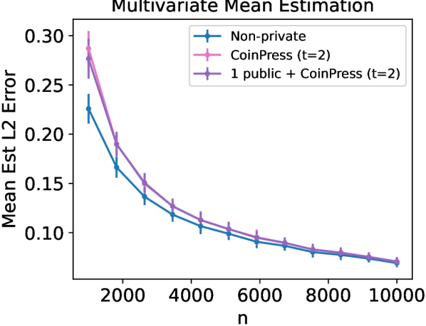
(a) $k=10$

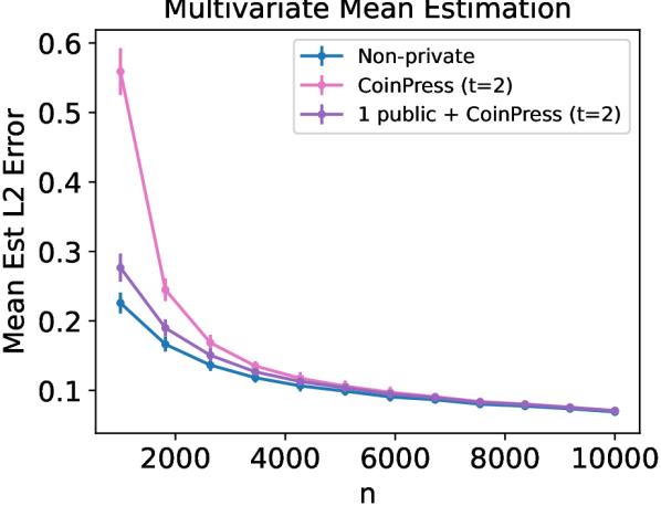
(b) $k=100$

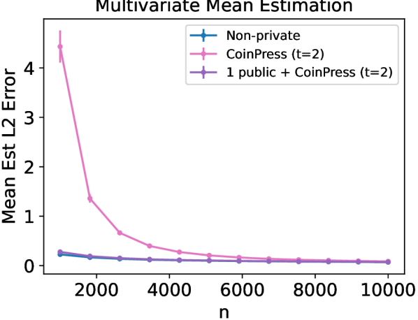
(c) $k=1000$

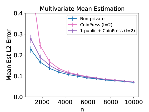
(d) $k=100$ (zoomed in)

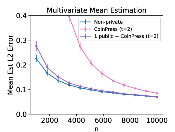
(e) $k=1000$ (zoomed in)

Figure 1: Comparing the error of CoinPress [BDKU20] under its best setting, against CoinPress with 1 public sample for mean estimation of $\mathcal{N}(k\cdot[1,...,1]^{T},I_{d})$ for $d=50$, targeting zCDP at $\rho=0.5$. Larger $k$ corresponds to weaker a priori bounds on the mean for CoinPress. For large $k$, a single public sample significantly improves results.

We examine the effect of $1$ public sample on the performance of CoinPress [BDKU20] with its best parameter setting ($t=2$), in a case where the initial a priori bounds on the mean are weak. Concretely, we draw $n$ samples from a $d=50$ dimensional Gaussian $\mathcal{N}(\mu_{k},I_{d})$, where $\mu_{k}=k\cdot[1,...,1]^{T}$ and correspondingly set our a priori bound $R=k\sqrt{d}$ for CoinPress. We show results for $k\in[10,100,1000]$, representing varying levels of strength in our a prior bounds on the mean.

We follow the evaluation protocol from [BDKU20]: we target zCDP with $\rho=0.5$, and at each sample size $n$ we run the estimator 100 times and report the $10\%$ trimmed mean of error from the ground truth (we additionally report the $10\%$ trimmed standard deviation as error bars). We also follow their practice of treating target failure probabilities $\beta_{i}$ of various steps of the algorithm as hyperparameters that can be tuned for the best empirical results. The new step we introduce (using the public sample to set $R$ based on $d,\beta$) uses $\beta=0.01$, which is the same value used for all the $\beta_{i}$’s in CoinPress.

The numerical result demonstrates the promise of utilizing public data for private data analysis, and confirms the takeaway that very little public data can help greatly when a priori knowledge of the private data is weak. As is visible from the plots, the error of our public-private algorithm tracks the non-private algorithm closer when a priori bounds on the mean are weak $(k=1000$ case).

Note that these results are only meant to be a proof-of-concept simulation to demonstrate the promise of public data – thorough tuning and evaluation of these algorithms (which is necessary to bring these algorithms to practice) is an important direction for future work.

References

• [AAK21] Ishaq Aden-Ali, Hassan Ashtiani and Gautam Kamath “On the Sample Complexity of Privately Learning Unbounded High-Dimensional Gaussians” In Proceedings of the 32nd International Conference on Algorithmic Learning Theory, ALT ’21 JMLR, Inc., 2021, pp. 185–216
• [ABM19] Noga Alon, Raef Bassily and Shay Moran “Limits of Private Learning with Access to Public Data” In Advances in Neural Information Processing Systems 32, NeurIPS ’19 Curran Associates, Inc., 2019, pp. 10342–10352
• [ACGMMTZ16] Martin Abadi, Andy Chu, Ian Goodfellow, H Brendan McMahan, Ilya Mironov, Kunal Talwar and Li Zhang “Deep Learning with Differential Privacy” In Proceedings of the 2016 ACM Conference on Computer and Communications Security, CCS ’16 New York, NY, USA: ACM, 2016, pp. 308–318
• [ADK19] Brendan Avent, Yatharth Dubey and Aleksandra Korolova “The Power of the Hybrid Model for Mean Estimation” In Proceedings on Privacy Enhancing Technologies 2020.4 Sciendo, 2019, pp. 48–68
• [AGMRSSSTT21] Ehsan Amid, Arun Ganesh, Rajiv Mathews, Swaroop Ramaswamy, Shuang Song, Thomas Steinke, Vinith M Suriyakumar, Om Thakkar and Abhradeep Thakurta “Public Data-Assisted Mirror Descent for Private Model Training” In arXiv preprint arXiv:2112.00193, 2021
• [AK01] Sanjeev Arora and Ravi Kannan “Learning mixtures of arbitrary Gaussians” In Proceedings of the 33rd Annual ACM Symposium on the Theory of Computing, STOC ’01 New York, NY, USA: ACM, 2001, pp. 247–257
• [AKZHL17] Brendan Avent, Aleksandra Korolova, David Zeber, Torgeir Hovden and Benjamin Livshits “BLENDER: Enabling Local Search with a Hybrid Differential Privacy Model” In 26th USENIX Security Symposium, USENIX Security ’17 USENIX Association, 2017, pp. 747–764
• [AL21] Hassan Ashtiani and Christopher Liaw “Private and polynomial time algorithms for learning Gaussians and beyond” In arXiv preprint arXiv:2111.11320, 2021
• [AM05] Dimitris Achlioptas and Frank McSherry “On Spectral Learning of Mixtures of Distributions” In Proceedings of the 18th Annual Conference on Learning Theory, COLT ’05 Springer, 2005, pp. 458–469
• [BCMNUW20] Raef Bassily, Albert Cheu, Shay Moran, Aleksandar Nikolov, Jonathan Ullman and Steven Wu “Private Query Release Assisted by Public Data” In Proceedings of the 37th International Conference on Machine Learning, ICML ’20 JMLR, Inc., 2020, pp. 695–703
• [BDKU20] Sourav Biswas, Yihe Dong, Gautam Kamath and Jonathan Ullman “CoinPress: Practical Private Mean and Covariance Estimation” In Advances in Neural Information Processing Systems 33, NeurIPS ’20 Curran Associates, Inc., 2020, pp. 14475–14485
• [BKSW19] Mark Bun, Gautam Kamath, Thomas Steinke and Zhiwei Steven Wu “Private Hypothesis Selection” In Advances in Neural Information Processing Systems 32, NeurIPS ’19 Curran Associates, Inc., 2019, pp. 156–167
• [BMN20] Raef Bassily, Shay Moran and Anupama Nandi “Learning from Mixtures of Private and Public Populations” In Advances in Neural Information Processing Systems 33, NeurIPS ’20 Curran Associates, Inc., 2020, pp. 2947–2957
• [BNS16] Amos Beimel, Kobbi Nissim and Uri Stemmer “Private Learning and Sanitization: Pure vs. Approximate Differential Privacy” In Theory of Computing 12.1, 2016, pp. 1–61
• [BNS16a] Mark Bun, Kobbi Nissim and Uri Stemmer “Simultaneous Private Learning of Multiple Concepts” In Proceedings of the 7th Conference on Innovations in Theoretical Computer Science, ITCS ’16 New York, NY, USA: ACM, 2016, pp. 369–380
• [BS16] Mark Bun and Thomas Steinke “Concentrated Differential Privacy: Simplifications, Extensions, and Lower Bounds” In Proceedings of the 14th Conference on Theory of Cryptography, TCC ’16-B Berlin, Heidelberg: Springer, 2016, pp. 635–658
• [BTGT18] Raef Bassily, Om Thakkar and Abhradeep Guha Thakurta “Model-Agnostic Private Learning” In Advances in Neural Information Processing Systems 31, NeurIPS ’18 Curran Associates, Inc., 2018, pp. 7102–7112
• [DKKLMS16] Ilias Diakonikolas, Gautam Kamath, Daniel M. Kane, Jerry Li, Ankur Moitra and Alistair Stewart “Robust Estimators in High Dimensions without the Computational Intractability” In Proceedings of the 57th Annual IEEE Symposium on Foundations of Computer Science, FOCS ’16 Washington, DC, USA: IEEE Computer Society, 2016, pp. 655–664
• [DMNS06] Cynthia Dwork, Frank McSherry, Kobbi Nissim and Adam Smith “Calibrating Noise to Sensitivity in Private Data Analysis” In Proceedings of the 3rd Conference on Theory of Cryptography, TCC ’06 Berlin, Heidelberg: Springer, 2006, pp. 265–284
• [DRV10] Cynthia Dwork, Guy N. Rothblum and Salil Vadhan “Boosting and Differential Privacy” In Proceedings of the 51st Annual IEEE Symposium on Foundations of Computer Science, FOCS ’10 Washington, DC, USA: IEEE Computer Society, 2010, pp. 51–60
• [DS01] K Davidson and Stanislaw J Szarek “Local operator theory, random matrices and Banach spaces, Handbook of the geometry of Banach spaces, Vol. I, 317–366” North-Holland, Amsterdam, 2001
• [DTTZ14] Cynthia Dwork, Kunal Talwar, Abhradeep Thakurta and Li Zhang “Analyze Gauss: Optimal Bounds for Privacy-Preserving Principal Component Analysis” In Proceedings of the 46th Annual ACM Symposium on the Theory of Computing, STOC ’14 New York, NY, USA: ACM, 2014, pp. 11–20
• [Ede88] Alan Edelman “Eigenvalues and Condition Numbers of Random Matrices” In SIAM J. Matrix Anal. Appl. 9.4 USA: Society for IndustrialApplied Mathematics, 1988, pp. 543–560 DOI: 10.1137/0609045
• [HKM22] Samuel B Hopkins, Gautam Kamath and Mahbod Majid “Efficient Mean Estimation with Pure Differential Privacy via a Sum-of-Squares Exponential Mechanism” In Proceedings of the 54th Annual ACM Symposium on the Theory of Computing, STOC ’22 New York, NY, USA: ACM, 2022
• [HW71] David Lee Hanson and Farroll Tim Wright “A Bound on Tail Probabilities for Quadratic Forms in Independent Random Variables” In The Annals of Mathematical Statistics 42.3 The Institute of Mathematical Statistics, 1971, pp. 1079–1083
• [JE13] Zhanglong Ji and Charles Elkan “Differential Privacy Based on Importance Weighting” In Machine Learning 93.1 Springer, 2013, pp. 163–183
• [KKMN09] Aleksandra Korolova, Krishnaram Kenthapadi, Nina Mishra and Alexandros Ntoulas “Releasing Search Queries and Clicks Privately” In Proceedings of the 18th International World Wide Web Conference, WWW ’09 New York, NY, USA: ACM, 2009, pp. 171–180
• [KLSU19] Gautam Kamath, Jerry Li, Vikrant Singhal and Jonathan Ullman “Privately Learning High-Dimensional Distributions” In Proceedings of the 32nd Annual Conference on Learning Theory, COLT ’19, 2019, pp. 1853–1902
• [KMSSU21] Gautam Kamath, Argyris Mouzakis, Vikrant Singhal, Thomas Steinke and Jonathan Ullman “A Private and Computationally-Efficient Estimator for Unbounded Gaussians” arXiv, 2021 DOI: 10.48550/ARXIV.2111.04609
• [KMV21] Pravesh K Kothari, Pasin Manurangsi and Ameya Velingker “Private Robust Estimation by Stabilizing Convex Relaxations” In arXiv preprint arXiv:2112.03548, 2021
• [KRRT21] Peter Kairouz, Mónica Ribero, Keith Rush and Abhradeep Thakurta “(Nearly) Dimension Independent Private ERM with AdaGrad Rates via Publicly Estimated Subspaces” In Proceedings of the 34th Annual Conference on Learning Theory, COLT ’21, 2021, pp. 2717–2746
• [KSSU19] Gautam Kamath, Or Sheffet, Vikrant Singhal and Jonathan Ullman “Differentially Private Algorithms for Learning Mixtures of Separated Gaussians” In Advances in Neural Information Processing Systems 32, NeurIPS ’19 Curran Associates, Inc., 2019, pp. 168–180
• [KV18] Vishesh Karwa and Salil Vadhan “Finite Sample Differentially Private Confidence Intervals” In Proceedings of the 9th Conference on Innovations in Theoretical Computer Science, ITCS ’18 Dagstuhl, Germany: Schloss Dagstuhl–Leibniz-Zentrum fuer Informatik, 2018, pp. 44:1–44:9
• [LKO21] Xiyang Liu, Weihao Kong and Sewoong Oh “Differential privacy and robust statistics in high dimensions” In arXiv preprint arXiv:2111.06578, 2021
• [LTLH22] Xuechen Li, Florian Tramèr, Percy Liang and Tatsunori Hashimoto “Large Language Models Can Be Strong Differentially Private Learners” In Proceedings of the 10th International Conference on Learning Representations, ICLR ’22, 2022
• [LVSUW21] Terrance Liu, Giuseppe Vietri, Thomas Steinke, Jonathan Ullman and Steven Wu “Leveraging Public Data for Practical Private Query Release” In Proceedings of the 38th International Conference on Machine Learning, ICML ’21 JMLR, Inc., 2021, pp. 6968–6977
• [LWAFF21] Zelun Luo, Daniel J Wu, Ehsan Adeli and Li Fei-Fei “Scalable Differential Privacy with Sparse Network Finetuning” In Proceedings of the 2021 IEEE Computer Society Conference on Computer Vision and Pattern Recognition, CVPR ’21 Washington, DC, USA: IEEE Computer Society, 2021, pp. 5059–5068
• [NB20] Anupama Nandi and Raef Bassily “Privately Answering Classification Queries in the Agnostic PAC Model” In Proceedings of the 31st International Conference on Algorithmic Learning Theory, ALT ’20 JMLR, Inc., 2020, pp. 687–703
• [PAEGT17] Nicolas Papernot, Martín Abadi, Ulfar Erlingsson, Ian Goodfellow and Kunal Talwar “Semi-supervised knowledge transfer for deep learning from private training data” In Proceedings of the 5th International Conference on Learning Representations, ICLR ’17, 2017
• [PCSTE19] Nicolas Papernot, Steve Chien, Shuang Song, Abhradeep Thakurta and Ulfar Erlingsson “Making the Shoe Fit: Architectures, Initializations, and Tuning for Learning with Privacy”, https://openreview.net/forum?id=rJg851rYwH, 2019
• [PSMRTE18] Nicolas Papernot, Shuang Song, Ilya Mironov, Ananth Raghunathan, Kunal Talwar and Úlfar Erlingsson “Scalable Private Learning with PATE” In Proceedings of the 6th International Conference on Learning Representations, ICLR ’18, 2018
• [SST06] Arvind Sankar, Daniel A. Spielman and Shang-Hua Teng “Smoothed Analysis of the Condition Numbers and Growth Factors of Matrices” In SIAM J. Matrix Anal. Appl. 28.2 USA: Society for IndustrialApplied Mathematics, 2006, pp. 446–476 DOI: 10.1137/S0895479803436202
• [TB21] Florian Tramèr and Dan Boneh “Differentially Private Learning Needs Better Features (or Much More Data)” In Proceedings of the 9th International Conference on Learning Representations, ICLR ’21, 2021
• [TCKMS21] Eliad Tsfadia, Edith Cohen, Haim Kaplan, Yishay Mansour and Uri Stemmer “FriendlyCore: Practical Differentially Private Aggregation” In arXiv preprint arXiv:2110.10132, 2021
• [VW02] Santosh Vempala and Grant Wang “A Spectral Algorithm for Learning Mixtures of Distributions” In Proceedings of the 43rd Annual IEEE Symposium on Foundations of Computer Science, FOCS ’02 Washington, DC, USA: IEEE Computer Society, 2002, pp. 113–123
• [Yu+22] Da Yu, Saurabh Naik, Arturs Backurs, Sivakanth Gopi, Huseyin A Inan, Gautam Kamath, Janardhan Kulkarni, Yin Tat Lee, Andre Manoel, Lukas Wutschitz, Sergey Yekhanin and Huishuai Zhang “Differentially Private Fine-tuning of Language Models” In Proceedings of the 10th International Conference on Learning Representations, ICLR ’22, 2022
• [YZCL21] Da Yu, Huishuai Zhang, Wei Chen and Tie-Yan Liu “Do Not Let Privacy Overbill Utility: Gradient Embedding Perturbation for Private Learning” In Proceedings of the 9th International Conference on Learning Representations, ICLR ’21, 2021
• [ZWB21] Yingxue Zhou, Zhiwei Steven Wu and Arindam Banerjee “Bypassing the Ambient Dimension: Private SGD with Gradient Subspace Identification” In Proceedings of the 9th International Conference on Learning Representations, ICLR ’21, 2021
• [ZZ18] Anru R. Zhang and Yuchen Zhou “On the Non-asymptotic and Sharp Lower Tail Bounds of Random Variables” arXiv, 2018 DOI: 10.48550/ARXIV.1810.09006