Light beam interacting with electron medium. Exact solutions of the model and their possible applications to photon entanglement problem

Abstract

We consider a model for describing a QED system consisting of a photon beam interacting with quantized charged spinless particles. We restrict ourselves by a photon beam that consists of photons with two different momenta moving in the same direction. Photons with each moment may have two possible linear polarizations. The exact solutions correspond to two independent subsystems, one of which corresponds to the electron medium and another one is described by vectors in the photon Hilbert subspace and is representing a set of some quasi-photons that do not interact with each other. In addition, we find exact solution of the model that correspond to the same system placed in a constant magnetic field. As an example, of possible applications, we use the solutions of the model for calculating entanglement of the photon beam by quantized electron medium and by a constant magnetic field. Thus, we calculate the entanglement measures (the information and the Schmidt ones) of the photon beam as functions of the applied magnetic field and parameters of the electron medium.

Keywords: Entanglement, two-qubit systems, magnetic field.

1 Introduction

Exactly solvable models in quantum mechanics and QFT play important role for understanding different physical phenomena, see e.g. Refs. [1, 2, 3, 4]. Here, we consider a model for describing a QED system consisting of a photon beam interacting with quantized charged spinless particles (Klein-Gordon particles that are called for simplicity electrons in what follows). We restrict ourselves by a photon beam that consists of photons with two different momenta $\mathbf{k}_{s}=\kappa_{s}\mathbf{n}$, $s=1,2$ (frequencies), moving in the same direction defined by a unit vector $\mathbf{n.}$ Photons with each moment may have two possible linear polarizations $\lambda=1,2$. In the beginning, we consider the electron subsystem consisting of one spinless particle. Both quantized fields (electromagnetic and the Klein-Gordon one) are placed in a box of the volume $V=L^{3}$ and periodic conditions are supposed. For such a model we find some exact solutions, see Sec. 2. In these solutions we interpret $\rho=V^{-1}$ as the electron density, believing that now the model describes the photon beam interacting with many charged spinless particles (particles that interact with the photon beam but do not interact with each other) the totality of which we call below the electron medium. The exact solutions correspond to two independent subsystems, one of which is the electron medium and another one is described by vectors in the photon Hilbert subspace and is representing a set of some quasi-photons that do not interact with each other. In addition, we find exact solution of the model that correspond to the same system placed in a constant magnetic field. As an example, we use the obtained solutions of the model for calculating entanglement of the photon beam by quantized electron medium and by a constant magnetic field, see 3. Some final remark can be found in Sec. 4. In the Appendix 6 we have placed a necessary technical information, which is used in analyzing entanglement in two-qubit systems.

2 Photon beam interacting with quantum spinless electron medium

2.1 General

We consider a model system which consists of a photon subsystem and a subsystem of quantized charged relativistic spinless particles (the Klein-Gordon particles). The photon subsystem under consideration (the photon beam) consists of a finite number of photons with linear polarizations moving in the same direction defined by a unit vector $\mathbf{n}$ (we assume that $\mathbf{n}$ is directed along the axis $z,$ i.e., $\mathbf{n}=(0,0,1)$. Here, we restrict ourselves by a photon beam that consists of photons with two different momenta $\mathbf{k}_{s}=\kappa_{s}\mathbf{n}$, $s=1,2$ (frequencies), photons with each moment may have two possible linear polarizations $\lambda=1,2$. We also suppose that particles from the electron medium interact with the photon beam but do not interact with each other. Both quantized fields (electromagnetic and the electron one) are placed in a box of the volume $V=L^{3}$ and periodic conditions are supposed. The later conditions imply that momenta of the photons of the beam are quantized,

$$\kappa_{s}=\kappa_{0}d_{s},\quad\kappa_{0}=2\pi L^{-1},\quad d_{s}\in\mathbb{N},\quad s=1,2\,.$$

The operator-valued potentials $\hat{A}^{\mu}(\mathbf{r})$, $\mathbf{r}=(x^{1},x^{2},x^{3}=z)$ of the hoton beam are chosen in the Coulomb gauge $\partial_{\mu}\hat{A}^{\mu}=0$ as: $\hat{A}^{\mu}(\mathbf{r})=(0,\mathbf{\hat{A}}(\mathbf{r}))$, $\operatorname{div}\mathbf{\hat{A}}(\mathbf{r})=0$. The nonzero vector potential depends, in fact, only on the coordinate $z$,

$$\mathbf{\hat{A}}\left(\mathbf{r}\right)=\mathbf{\hat{A}}\left(z\right)=\sum_{s=1,2}\sum_{\lambda=1,2}\sqrt{\frac{1}{2\kappa_{s}V}}\left\{\hat{a}_{s\mathbf{,}\lambda}\exp\left[i\kappa_{s}z\right]+\hat{a}_{s\mathbf{,}\lambda}^{\dagger}\exp\left[-i\kappa_{s}z\right]\right\}\mathbf{e}_{\lambda}\,.$$

Here $\hat{a}_{s,\lambda}$ and $\hat{a}_{s,\lambda}^{\dagger}$ are free photon creation and annihilation operators satisfying Bose-type commutation relations:

$$\left[\hat{a}_{s\mathbf{,}\lambda},\hat{a}_{s^{\prime},\lambda^{\prime}}\right]=0,\ \left[\hat{a}_{s\mathbf{,}\lambda},\hat{a}_{s^{\prime},\lambda^{\prime}}^{\dagger}\right]=\delta_{s,s^{\prime}}\delta_{\lambda,\lambda^{\prime}},\ s,s^{\prime}=1,2,\ \ \lambda,\lambda^{\prime}=1,2\,,d$$

where $\mathbf{e}_{\lambda}$ are real polarization vectors, $(\mathbf{e}_{\lambda}\mathbf{e}_{\lambda^{\prime}})=\delta_{\lambda,\lambda^{\prime}}$, $(\mathbf{ne}_{\lambda})=0$. The photon operators are acting in a photon Fock space $\mathfrak{H}_{\mathrm{\gamma}}$ constructing by the creation and annihilation operators and a vacuum vector $\left|0\right\rangle_{\mathrm{\gamma}}$, $\hat{a}_{s,\lambda}\left|0\right\rangle_{\mathrm{\gamma}}=0$, $\forall s,\lambda$. Vectors from the photon Fock space are denoted by $\left|\Psi\right\rangle_{\mathrm{\gamma}}$, $\left|\Psi\right\rangle_{\mathrm{\gamma}}\in\mathfrak{H}_{\mathrm{\gamma}}$.

The free photon Hamiltonian has the form:

$$\hat{H}_{\mathrm{\gamma}}=\sum_{s=1,2}\sum_{\lambda=1,2}\kappa_{s}\hat{a}_{s,\lambda}^{\dagger}\hat{a}_{s,\lambda}\,.$$

On the quantum level, electrons are described by a scalar field $\varphi(\mathbf{r})$ (the Klein-Gordon field) interacting with a classical external electromagnetic field of the form $A_{\mathrm{ext}}^{\mu}(\mathbf{r})=(A_{\mathrm{ext}}^{0}=0,\mathbf{A}_{\mathrm{ext}}(r))$, $\mathbf{A_{\mathrm{ext}}(r})=(A\mathbf{{}_{\mathrm{ext}}}^{k}(\mathbf{r}))$, $\mu=0,\dots,3$, $k=1,2,3$. We suppose that this field does not violate the vacuum stability, see [5, 6]. After canonical quantization (see [7, 6]) the scalar field and its canonical momentum $\pi(\mathbf{r})$ become operators $\hat{\varphi}(\mathbf{r})$ and $\hat{\pi}(\mathbf{r}).$ The corresponding Heisenberg operators $\hat{\varphi}(x)$ and $\hat{\pi}(x)$, $x=(x^{\mu})=(x^{0}=t,\mathbf{r})$, satisfy equal-time nonzero commutation relations:

$$[\hat{\varphi}(x),\hat{\pi}(x^{\prime})]_{t=t^{\prime}}=i\delta(\mathbf{r}-\mathbf{r}^{\prime})\,.$$ (1)

The scalar field operators are acting in an electron Fock space $\mathfrak{H}_{\mathrm{e}}$ constructed by a set of creation and annihilation operators of scalar particles interacting with the external field and by a corresponding vacuum vector $\left|0\right\rangle_{\mathrm{e}}$, see e.g. the two latter references. Vectors from the electron Fock space are denoted as $\left|\Psi\right\rangle_{\mathrm{e}}\subset\mathfrak{H}_{\mathrm{e}}$. The Fock space $\mathfrak{H}$ of the complete system is a tensor product of the photon Fock space and the electron Fock space, $\mathfrak{H=H}_{\mathrm{\gamma}}\otimes\mathfrak{H}_{\mathrm{e}}$. Vectors from the Fock space $\mathfrak{H}$ are denoted by $\left|\Psi\right\rangle$ such that, $\left|\Psi\right\rangle\in\mathfrak{H}$.

The Hamiltonian of the complete system has the following form (see, e.g. [6]):

$$\hat{H} = \int\left\{\hat{\pi}^{+}(\mathbf{r})\hat{\pi}(\mathbf{r})+\hat{\varphi}^{+}\left(\mathbf{r}\right)\left[\mathbf{\hat{P}}_{\mathrm{\gamma}}^{2}(\mathbf{r})+m^{2}\right]\hat{\varphi}\left(\mathbf{r}\right)\right\}d\mathbf{r}+\hat{H}_{\mathrm{\gamma}}\ ,$$

$$\mathbf{\hat{P}}_{\mathrm{\gamma}}(\mathbf{r}) = \mathbf{\hat{p}}+e\left[\mathbf{\hat{A}(}z)+\mathbf{A_{\mathrm{ext}}(r})\right]\,.$$ (2)

Here $m$ is the electron mass and $e>0$ is the absolute value of the electron charge.

Consider the amplitude

$$\varphi_{\mathrm{\gamma}}(x)=\ _{\mathrm{e}}\left\langle 0\right|\hat{\varphi}(\mathbf{r})\left|\boldsymbol{\Psi}\left(t\right)\right\rangle,\,$$ (3)

which is the projection of the vector $\left|\mathbf{\Psi}(t)\right\rangle$ onto a one-electron state remaining at the same time an abstract vector in the photon Fock space. We interpret $\varphi_{\mathrm{\gamma}}(x)$ as a state vector of photons interacting with an electron. In similar manner, one can introduce many-electron or positron amplitudes and interpreted them as state vectors of photons interacting with many charged particles.

To derive an equation for the state vector (3) we take into account that has the vector $\left|\mathbf{\Psi}(t)\right\rangle$ satisfies the Schrödinger equation with the Hamiltonian (2),

$$i\partial_{t}\left|\boldsymbol{\Psi}\left(t\right)\right\rangle=\hat{H}\left|\boldsymbol{\Psi}\left(t\right)\right\rangle\,.$$ (4)

Then with account taken of both Eqs. (3) and (4) and the commutation relations (1), we obtain:

$$\ i\partial_{t}\varphi_{\mathrm{\gamma}}(x) = \ {}_{\mathrm{e}}\left\langle 0\right|\hat{\varphi}(\mathbf{r})\hat{H}\left|\boldsymbol{\Psi}\left(t\right)\right\rangle=\ _{\mathrm{e}}\left\langle 0\right|\hat{H}\hat{\varphi}(\mathbf{r})+\left[\hat{\varphi}(\mathbf{r}),\hat{H}\right]\left|\boldsymbol{\Psi}\left(t\right)\right\rangle$$

$$= \chi_{\mathrm{\gamma}}(x)+\hat{H}_{\mathrm{\gamma}}\varphi_{\mathrm{\gamma}}(x)+\Delta\ ,\ \ \chi_{\mathrm{\gamma}}(x)=i\ _{\mathrm{e}}\left\langle 0\right|\hat{\pi}^{+}(\mathbf{r})\left|\boldsymbol{\Psi}\left(t\right)\right\rangle\,,$$ (5)

where the vector $\chi_{\mathrm{\gamma}}(x)$ satisfies the following equation

$$\ i\partial_{t}\chi_{\mathrm{\gamma}}(x) = i\ _{\mathrm{e}}\left\langle 0\right|\hat{\pi}^{+}(\mathbf{r})\hat{H}\left|\boldsymbol{\Psi}\left(t\right)\right\rangle=i\ _{\mathrm{e}}\left\langle 0\right|\hat{H}\hat{\pi}^{+}(\mathbf{r})+\left[\hat{\pi}^{+}(\mathbf{r}),\hat{H}\right]\left|\boldsymbol{\Psi}\left(t\right)\right\rangle$$ (6)

$$= \left[\mathbf{\hat{P}}_{\mathrm{\gamma}}^{2}(\mathbf{r})+m^{2}\right]\varphi_{\mathrm{\gamma}}(x)+\hat{H}_{\mathrm{\gamma}}\chi_{\mathrm{\gamma}}(x)+\Delta\,,$$

and the vector $\Delta$ contains many-particle amplitudes that are related to processes of virtual pair creation. We note that the vector $\Delta$ contains higher-order contributions in the fine structure constant. That is why, we neglect this term in what follows. With $\Delta=0$ equations (5) and (6) are reduced to a set of two coupled equations for the vectors $\chi_{\mathrm{\gamma}}(x)$ and $\varphi_{\mathrm{\gamma}}(x)$. This set implies the following second-order equation for the vector $\varphi_{\mathrm{\gamma}}(x)$:

$$\left[(i\partial_{t}-\hat{H}_{\mathrm{\gamma}})^{2}-\mathbf{\hat{P}}_{\mathrm{\gamma}}^{2}(\mathbf{r})-m^{2}\right]\varphi_{\mathrm{\gamma}}(x)=0\,.$$ (7)

It is convenient to pass from the vector $\varphi_{\mathrm{\gamma}}(x)$ to a vector $\Phi_{\mathrm{\gamma}}(x)$,

$$\Phi_{\mathrm{\gamma}}(x)=\exp\left(i\hat{H}_{\mathrm{\gamma}}t\right)\varphi_{\mathrm{\gamma}}(x)\,.$$

As it follows from Eq. (7) the vector $\Phi_{\mathrm{\gamma}}(x)$ satisfies a Klein-Gordon like equation:

$$\left(\hat{P}_{\mu}\hat{P}^{\mu}-m^{2}\right)\Phi_{\mathrm{\gamma}}(x)=0\ ,$$ (8)

$$\hat{P}^{\mu}=i\partial^{\mu}+e\left[\hat{A}^{\mu}(u)+A_{\mathrm{ext}}^{\mu}(\mathbf{r})\right]\ ,\ \hat{A}^{\mu}(u)=\left(0,\mathbf{\hat{A}}(u)\right)\ ,$$

$$\mathbf{\hat{A}}(u)=\frac{1}{e}\sum_{s=1,2}\sum_{\lambda=1,2}\sqrt{\frac{\varepsilon}{2\kappa_{s}}}\left[\hat{a}_{s,\lambda}\exp\left(-i\kappa_{s}u\right)+\hat{a}_{s,\lambda}^{\dagger}\exp\left(i\kappa_{s}u\right)\right]\mathbf{e}_{\lambda}\ ,$$

$$\ u=t-z,\ \partial_{\mu}=\left(\partial_{t},\mathbf{\nabla}\right),\ \varepsilon=\alpha\rho,\ \alpha=e^{2}/\hbar c=1/137\,.$$

As was already said, we interpret $\rho=V^{-1}=L^{-3}$ as the electron media density. The quantity $\varepsilon$ characterizes the strength of the interaction between the quantum charged particles and the photon beam.

2.2 The system in the absence of an external field

First we consider the case without the external electromagnetic field, $A_{\mathrm{ext}}^{\mu}(\mathbf{r})=0$. Then equation (8) admits the following integrals of motion:

$$\left[\hat{G}_{\nu},\left(\hat{P}_{\mu}\hat{P}^{\mu}-m^{2}\right)\right]=0,\ \ \hat{G}_{\nu}=i\partial_{\nu}+n_{\nu}\hat{H}_{\mathrm{\gamma}},\ \ n^{\mu}=(1,0,0,1)\ ,$$

$$[\hat{G}_{\mu},\hat{G}_{\nu}]=0\ ,\ \ [\hat{G}_{\mu},\hat{P}_{\nu}]=0,\ \mu,\nu=0,1,2,3\,.$$ (9)

In this case, we look for solutions of Eq. (8) that are eigenvectors for the operators $\hat{G}_{\mu}$,

$$\hat{G}_{\mu}\Phi_{\mathrm{\gamma}}(x)=g_{\mu}\Phi_{\mathrm{\gamma}}(x)\,.$$ (10)

With account taken of Eqs. (10) such solutions $\Phi_{\mathrm{\gamma}}(x)$ satisfy the following equation:

$$\left[\hat{H}_{\mathrm{K}}-\frac{g^{2}-m^{2}}{2(ng)}\right]\Phi_{\mathrm{\gamma}}(x)=0,\ \ \hat{H}_{\mathrm{K}}=\hat{H}_{\mathrm{\gamma}}+\frac{e\left(\mathbf{p\hat{A}}\right)}{\left(ng\right)}+\frac{e^{2}\mathbf{\hat{A}}^{2}}{2\left(ng\right)}\,,$$

where $ng=g_{0}+g_{3}$. The latter fact implies that the operator $\hat{H}_{\mathrm{K}}$ commutes with the one $\hat{P}_{\mu}\hat{P}^{\mu}-m$ on solutions, which means:

$$\left[\hat{H}_{\mathrm{K}},\left(\hat{P}_{\mu}\hat{P}^{\mu}-m^{2}\right)\right]\Phi_{\mathrm{\gamma}}(x)=0\,,$$

and therefore the operator $\hat{H}_{\mathrm{K}}$ is also an integral of motion. The operator $\hat{G}_{\mu}\,$can be represented in the form:

$$\hat{G}_{\mu}=(\hat{P}_{\mathrm{K}})_{\mu}+n_{\mu}\hat{H}_{\mathrm{K}},\ \ (\hat{P}_{\mathrm{K}})_{\mu}=i\partial_{\mu}-n_{\mu}\left(\hat{H}_{\mathrm{K}}-\hat{H}_{\mathrm{\gamma}}\right)\,.$$ (11)

Since the operator $(\hat{P}_{\mathrm{K}})_{\mu}$ is a linear combinations of the integrals of motion $\hat{G}_{\mu}$ and $\hat{H}_{\mathrm{K}}$, it also is an integral of motion.

Thus, we may find solutions of Eqs. (8) and (10), that are at the same time eigenvectors of the integrals of motion $(\hat{P}_{\mathrm{K}})_{\mu}$ and $\hat{H}_{\mathrm{K}}$:

$$(\hat{P}_{\mathrm{K}})_{\mu}\ \Phi_{\mathrm{\gamma}}(x) = p_{\mu}\Phi_{\mathrm{\gamma}}(x)\ ,$$

$$\hat{H}_{\mathrm{K}}\Phi_{\mathrm{\gamma}}(x) = E_{\mathrm{ph}}\Phi_{\mathrm{\gamma}}(x)\,.$$ (12)

This consideration becomes consistent if $p^{2}=p_{0}^{2}+\mathbf{p}^{2}=m^{2}$. Without loss of generality, we can set $\mathbf{p}_{\perp}=(p^{1},p^{2})=0$ in the case under consideration. Then $(ng)=(np)=p_{0}+p_{3}$. Besides, it follows from the above equations that

$$g_{\mu}=p_{\mu}+n_{\mu}E_{\mathrm{ph}}\Longrightarrow g_{0}=p_{0}+E_{\mathrm{ph}},\ \ g_{3}=p_{3}-E_{\mathrm{ph}}\,.$$ (13)

The operator $\hat{G}^{\mu}$ can be interpreted as a four-momentum operator of an electron and the photon beam and its eigenvalues $g_{\mu}$ as the energy-momentum of such a system. Switching off the electron-photon interaction, $\hat{G}^{\mu}$ is reduced to the sum of the energy momentum operator $i\partial_{\mu}$ of the electron and of the energy-momentum operator of the photon beam $n_{\mu}\hat{H}_{\mathrm{\gamma}}$. Thus, the system splits into two independent subsystems - a system of quasi-photons and a system of electrons, so that the energy-momentum vector of the system $g^{\mu}$ is the sum (13) of the energy-momentum $p^{\mu}$ of an electron and the momentum energy of the quasi-photons $n^{\mu}E_{\mathrm{ph}}$.

Solving Eq. (10), we represent the vector $\Phi_{\mathrm{\gamma}}(x)$ in the following form:

$$\Phi_{\mathrm{\gamma}}(x)=\hat{U}\Phi_{\mathrm{\gamma}}^{\left(1\right)}(x),\ \ \hat{U}=\exp\left(i\hat{H}_{\mathrm{\gamma}}u\right)\,.$$ (14)

Since $\hat{U}^{\dagger}\hat{G}_{\mu}\hat{U}=i\partial_{\mu}$, we obtain:

$$i\partial_{\mu}\Phi_{\mathrm{\gamma}}^{\left(1\right)}(x)=g_{\mu}\Phi_{\mathrm{\gamma}}^{\left(1\right)}(x)\Longrightarrow\Phi_{\mathrm{\gamma}}^{\left(1\right)}(x)=\exp\left(-igx\right)\Phi_{\mathrm{ph}}\,,$$

where the vector $\Phi_{\mathrm{ph}}\in\mathfrak{H}_{\mathrm{\gamma}}$ does not depend on $x$.

With account taken of Eqs. (14) and (12) as well as the operator relation $\hat{Q}^{\mu}=eU^{\dagger}\hat{A}^{\mu}\left(u\right)U=e\hat{A}^{\mu}\left(0\right)=(0,\mathbf{\hat{Q}})$, one can verify that the vector $\Phi_{\mathrm{ph}}$ satisfies the stationary Schrödinger equation:

$$\hat{H}_{\mathrm{ph}}\Phi_{\mathrm{ph}}=E_{\mathrm{ph}}\Phi_{\mathrm{ph}}\ ,\ \hat{H}_{\mathrm{ph}}=\hat{U}^{\dagger}\hat{H}_{\mathrm{K}}\hat{U}=\hat{H}_{\mathrm{\gamma}}+\frac{\mathbf{\hat{Q}}^{2}}{2\left(np\right)}\,.$$ (15)

Let us perform a linear canonical transformation from the free photon creation and annihilation operators $\hat{a}^{\dagger}$ and $\hat{a}$ to new creation and annihilation operators $\hat{c}^{\dagger}$ and $\hat{c}$,

$$\hat{a}=u\hat{c}-v\hat{c}^{\dagger},\ \ \hat{a}^{\dagger}=\hat{c}^{\dagger}u^{\dagger}-\hat{c}v^{\dagger},\ [\hat{c}_{s,\lambda},\hat{c}_{s^{\prime},\lambda^{\prime}}^{\dagger}]=\delta_{s,s^{\prime}}\delta_{\lambda,\lambda^{\prime}}\,,$$ (16)

where $uu^{\dagger}-vv^{\dagger}=1$ and $vu^{T}-uv^{T}=0$. We call the operators $\hat{c}^{\dagger}$ and $\hat{c}$ quasi-photon operators in what follows.

First of all, we choose the matrices $u=(u_{s,\lambda;s^{\prime},\lambda^{\prime}})$, $v=(v_{s,\lambda;s^{\prime},\lambda^{\prime}})$ to vanish all the terms linear in the quasi-photon operators in the Hamiltonian $\hat{H}_{\mathrm{ph}}$. Such matrices $u$ and $v$ and the column $\gamma$ have the form:

$$u_{s,\lambda;s^{\prime},\lambda^{\prime}}=u_{s,s^{\prime}}\delta_{\lambda,\lambda^{\prime}},\ \ v_{s,\lambda;s^{\prime},\lambda^{\prime}}=v_{s,s^{\prime}}\delta_{\lambda,\lambda^{\prime}}\ ,$$

$$u_{s,s^{\prime}}=F_{s,s^{\prime}}^{+}q_{s,s^{\prime}},\ \ v_{s,s^{\prime}}=F_{s,s^{\prime}}^{-}q_{s,s^{\prime}},\ \ F_{s,s^{\prime}}^{\pm}=\frac{1}{2}\left(\sqrt{\frac{\tau_{s^{\prime}}}{\kappa_{s}}}\pm\sqrt{\frac{\kappa_{s}}{\tau_{s^{\prime}}}}\right)\ ,$$

$$q_{s,s^{\prime}}=\frac{q_{s^{\prime}}}{\tau_{s^{\prime}}^{2}-\kappa_{s}^{2}},\ \ q_{s}\sqrt{\sum_{l=1,2}\left(\tau_{s}^{2}-\kappa_{l}^{2}\right)^{-2}}=1,\quad s=1,2\,,$$ (17)

where the quantities $\tau_{s}$ are roots of the algebraic equation

$$\epsilon\sum_{l=1,2}\left(\tau_{s}^{2}-\kappa_{l}^{2}\right)^{-1}=1,\ \ \epsilon=\varepsilon/\left(np\right)\,.$$ (18)

Note that there is no summation over the repeated indices in Eqs. (17).

Hamiltonian (15) is diagonal with respect to the operators $\hat{a}_{s\mathbf{,}\lambda}^{\dagger}$ and $\hat{a}_{s\mathbf{,}\lambda}$ at $\epsilon=0$. That is why we chose roots of equation (18) to satisfy the conditions $r_{s}^{2}(\epsilon=0)=\kappa_{s}^{2}$. Thus, we obtain:

$$\tau_{1}^{2} =A+B,\ r_{2}^{2}=A-B,\ A=\epsilon+\frac{\kappa_{1}^{2}+\kappa_{2}^{2}}{2}\ ,$$

$$\ B =\mathrm{sgn}(\kappa_{1}-\kappa_{2})\sqrt{\epsilon^{2}+\left(\frac{\kappa_{1}^{2}-\kappa_{2}^{2}}{2}\right)^{2}}\,,$$

where $\mathrm{sgn}(x)=1$, $x\geq 0$, and $\mathrm{sgn}(x)=-1$, $x<0$.

In terms of the quasi-photon operators, Hamiltonian (15) takes the form:

$$\hat{H}_{\mathrm{ph}}=\sum_{s=1,2}\sum_{\lambda=1,2}\tau_{s}\hat{c}_{s,\lambda}^{\dagger}\hat{c}_{s,\lambda}+H_{0},\ H_{0}=\sum_{s=1,2}\left(\tau_{s}-\kappa_{s}\right),\ \ \tau_{s}>0\,.$$

The eigenvalue problem (15) has the following solution:

$$E_{\mathrm{ph}} = \sum_{s=1,2}\sum_{\lambda=1,2}\tau_{s}N_{s,\lambda}+H_{0}\ ,\ N_{s,\lambda}\in\mathbb{N}\ ,$$

$$\left|\Phi_{\mathrm{ph}}\right\rangle = \left[\prod_{\lambda=1,2}\frac{\left(\hat{c}_{1,\lambda}^{\dagger}\right)^{N_{1,\lambda}}}{\sqrt{N_{1,\lambda}!}}\left|0_{1}\right\rangle_{c}\right]\otimes\left[\prod_{\lambda^{\prime}=1,2}\frac{\left(\hat{c}_{2,\lambda^{\prime}}^{\dagger}\right)^{N_{2,\lambda^{\prime}}}}{\sqrt{N_{2,\lambda^{\prime}}!}}\left|0_{2}\right\rangle_{c}\right]\,,$$ (19)

where $\left|0_{s}\right\rangle_{c}$ are partial vacua of the quasi-photon of the first ($s=1$) and the second kind ($s=2$), respectively.

Let us consider the case where the parameter $\epsilon$ is small, in particular,

$$\epsilon\ll\Delta\kappa=\left|\kappa_{2}-\kappa_{1}\right|\,.$$ (20)

Then approximate solutions of the characteristic equation (18) read:

$$r_{s}=\kappa_{s}+\frac{\epsilon}{2\kappa_{s}}+\frac{2\kappa_{s}+\kappa_{1}^{2}+\kappa_{2}^{2}}{8\kappa_{s}^{3}}\sum_{l\neq s}\frac{\epsilon^{2}}{\kappa_{s}^{2}-\kappa_{l}^{2}}+O(\epsilon^{3})\,,$$

such that:

$$u_{s,s^{\prime}} = \delta_{s,s^{\prime}}+\frac{(1-\delta_{s,s^{\prime}})\epsilon}{2\sqrt{\kappa_{1}\kappa_{2}}(\kappa_{s^{\prime}}-\kappa_{s})}+O(\epsilon^{2}),$$

$$v_{s,s^{\prime}} = \frac{\epsilon}{2\sqrt{\kappa_{1}\kappa_{2}}(\kappa_{s^{\prime}}+\kappa_{s})}+O(\epsilon^{2})\,.$$ (21)

2.3 The system in a constant uniform magnetic field

Here we consider the system under consideration placed in the external constant and uniform magnetic field $\mathbf{B}$ directed along the photon beam, $\mathbf{B}=(0,0,B>0)$. In fact, the external field affects directly only electrons, but then, due to the electron–photon interaction, it affects photons as well.

The Hamiltonian of the system has the form (2), where $\mathbf{A_{\mathrm{ext}}(r})$ is the vector potential of the constant magnetic field taken in the Landau gauge, $\mathbf{A}_{\mathrm{ext}}(\mathbf{r})=(-Bx^{2},0,0)$. In this case, equation (8) admits three integrals of motion $\hat{G}_{\mu}$, $\mu=0$, $1$, $3$, where $\hat{G}_{\mu}$ are given by Eqs. (9). Then we look for solutions of Eq. (8) that are eigenvectors for the integrals of motion,

$$\hat{G}_{\mu}\Phi_{\mathrm{\gamma}}(x)=g_{\mu}\Phi_{\mathrm{\gamma}}(x),\ \ \mu=0,1,3\,.$$ (22)

With account taken of Eqs. (22) one can see that vectors $\Phi_{\mathrm{\gamma}}(x)$ satisfy the following equation:

$$\left[\hat{H}_{\mathrm{K}}^{\prime}-\frac{g_{0}-g_{3}}{2}\right]\Phi_{\mathrm{\gamma}}(x)=0\ ,$$ (23)

$$\ \hat{H}_{\mathrm{K}}^{\prime}=\hat{H}_{\mathrm{\gamma}}+\frac{1}{2(ng)}\left\{\left[eBx^{2}-g^{1}-e\hat{A}^{1}(u)\right]^{2}+\left[i\partial_{2}-e\hat{A}^{2}(u)\right]^{2}+m^{2}\right\}\,.$$

The latter fact implies that the operator $\hat{H}_{\mathrm{K}}^{\prime}$ commutes with the operator $\hat{P}_{\mu}\hat{P}^{\mu}-m$ on solutions of Eq. (23), therefore, it is also an integral of motion.

Let us suppose that vectors $\Phi_{\mathrm{\gamma}}(x)$ are solutions of the eigenvalue problem

$$\hat{H}_{\mathrm{K}}^{\prime}\Phi_{\mathrm{\gamma}}(x)=E_{\mathrm{K}}\Phi_{\mathrm{\gamma}}(x)\,.$$ (24)

Then Eq. (23) is satisfies identically, if $g_{0}=E_{\mathrm{K}}+ng/2$. It follows from Eq. (22) that

$$\Phi_{\mathrm{\gamma}}(x)=\exp\left[-i(g_{0}t+g_{1}x^{1}+g_{3}z)\right]\hat{U}\Phi_{\mathrm{K}}(x^{2})\,,$$ (25)

where the operator $\hat{U}$ is given by Eq. (14). Substituting Eq. (25) into Eq. (24), we obtain:

$$\hat{H}_{\mathrm{K}}\Phi_{\mathrm{K}}(x^{2})=E_{\mathrm{K}}\Phi_{\mathrm{K}}(x^{2})\ ,$$

$$\hat{H}_{\mathrm{K}}=\hat{H}_{\mathrm{\gamma}}+\frac{1}{2(ng)}\left[\left(eBx^{2}-g^{1}-\hat{Q}^{1}\right)^{2}+(i\partial_{2}-\hat{Q}^{2})^{2}+m^{2}\right]\,.$$ (26)

The operator $\hat{G}_{\mu}$ can be represented in the form (11), where the operator $\hat{H}_{\mathrm{K}}$ is given by Eq. (26). We may find solutions of Eqs. (8) and (22), that are at the same time eigenvectors of the integrals of motion $(\hat{P}_{\mathrm{K}})_{\mu}$ and $\hat{H}_{\mathrm{K}}$:

$$(\hat{P}_{\mathrm{K}})_{\mu}\ \Phi_{\mathrm{\gamma}}(x) = p_{\mu}\Phi_{\mathrm{\gamma}}(x),\ \ \ \ \mu=0,1,3\ ,$$ (27)

$$\hat{H}_{\mathrm{K}}\Phi_{\mathrm{\gamma}}(x) = E_{\mathrm{ph}}\Phi_{\mathrm{\gamma}}(x)\,,$$ (28)

It follows from Eqs. (22) and (27)-(28) that

$$g_{0}=p_{0}+E_{\mathrm{ph}},\ \ g_{1}=p_{1},\ \ g_{3}=p_{3}-E_{\mathrm{ph}},\ \ ng=np\,.$$

At this stage, we, following the pioneer work by Malkin and Man‘ko [8], introduce new creation $\hat{c}_{0}^{\dagger}$ and annihilation $\hat{c}_{0}$ operators, $[\hat{c}_{0},\hat{c}_{0}^{\dagger}]=1$,

$$\hat{c}_{0}=(2)^{-1/2}\left(\eta+\partial_{\eta}\right),\ \ \hat{c}_{0}^{\dagger}=(2)^{-1/2}\left(\eta-\partial_{\eta}\right),\ (eB)^{1/2}\eta=\left(eBx^{2}-g^{1}\right)\ ,$$

$$x^{2}=\sqrt{\frac{1}{2eB}}\left(\hat{c}_{0}-\hat{c}_{0}^{\dagger}\right)+g^{1},\ \ \partial_{2}=\sqrt{\frac{eB}{2}}\left(\hat{c}_{0}+\hat{c}_{0}^{\dagger}\right)\,,$$

that, in fact, describe circular motion of charged particles in the magnetic field. The latter operators commute with all the quasi-photon operators $\hat{c}_{s\mathbf{,}\lambda}$ and $\hat{c}_{s^{\prime},\lambda^{\prime}}^{\dagger}$, $s,s^{\prime}=1,2$. It is convenient to introduce the operators $\hat{c}_{0,\lambda}^{\dagger}=\hat{c}_{0}^{\dagger}\delta_{\lambda,1}$ and $\hat{c}_{0,\lambda}=\hat{c}_{0}\delta_{\lambda,1}$.

One can see that the Hamiltonian $\hat{H}_{\mathrm{K}}$ is a quadratic operator with respect to the extended set of creation $\hat{c}_{s,\lambda}^{\dagger}$ and annihilation $\hat{c}_{s,\lambda}$, $s=0,1,2$,$\ \lambda=1,2$ operators. Then with the help of the linear canonical transformation (16), one can diagonalize the Hamiltonian $\hat{H}_{\mathrm{K}}$. The diagonalized Hamiltonian is represented as a sum of two commuting terms, the one $H_{\mathrm{e}}$ corresponds to the electron subsystem, while the second one $H_{\mathrm{ph}}$ to the subsystem of the quasi-photons,

$$\hat{H}_{\mathrm{K}} = H_{\mathrm{ph}}+H_{\mathrm{e}},\ \ H_{\mathrm{e}}=\tau_{0}\hat{c}_{0}^{\dagger}\hat{c}_{0}+\left[m^{2}(np)^{-1}-\omega\right]/2,\ \omega=eB(np)^{-1}\ ,\$$

$$H_{\mathrm{ph}} = \sum_{s=1,2}\sum_{\lambda=1,2}\tau_{s}c_{s,\lambda}^{\dagger}c_{s,\lambda}-\sum_{s=1,2}\sum_{\lambda,\lambda^{\prime}=1,2}\tau_{k,\lambda^{\prime}}\left|v_{s,\lambda;k,\lambda^{\prime}}\right|^{2}+\frac{\epsilon}{2}\left(\kappa_{1}^{-1}+\kappa_{2}^{-1}\right)\,.$$

Eigenvalues $E_{\mathrm{K}}$ and $E_{\mathrm{ph}}$ are:

$$E_{\mathrm{K}} = E_{\mathrm{ph}}+\tau_{0}N_{0}\ +\left[m^{2}(np)^{-1}+\omega\right]/2\,,$$

$$E_{\mathrm{ph}} = \sum_{s=1,2}\sum_{\lambda=1,2}\tau_{s}N_{s,\lambda}+H_{0},\ N_{0}\in\mathbb{N},\ \ N_{s,\lambda}\in\mathbb{N}\,.$$ (29)

With account taken of Eqs. (29), we obtain from the equation $g_{0}=E_{\mathrm{K}}+np/2$ that

$$p_{0}^{2}=eB\left(2\frac{\tau_{0}}{\omega}N_{0}+1\right)+p_{3}^{2}+m^{2}\,.$$

Quantities $r_{k,\lambda}$ are positive roots of the equation

$$\sum_{s=1,2}\frac{\epsilon}{\tau_{k,\lambda}^{2}-\kappa_{s}^{2}}=1+\frac{\left(-1\right)^{\lambda-1}\omega}{\tau_{k,\lambda}},\ \ \tau_{0,\lambda}=\tau_{0}\delta_{\lambda,1},\ \ k=0,1,2\,,$$ (30)

satisfying the conditions $\tau_{k,\lambda}(\epsilon=0)=\kappa_{s}$.

In what follows, we only need explicit expressions for the matrices $u_{s,\lambda;k,\lambda^{\prime}}$ and $v_{s,\lambda;k,\lambda^{\prime}}$ with $s,k=1,2$, and $\lambda=1,2$. They are:

$$u_{s,\lambda;k,\lambda^{\prime}} = \left[\left(\sqrt{\frac{\tau_{k,\lambda^{\prime}}}{\kappa_{s}}}+\sqrt{\frac{\kappa_{s}}{\tau_{k,\lambda^{\prime}}}}\right)\frac{(-1)^{\lambda^{\prime}-1}\delta_{\lambda,1}-i\delta_{\lambda,2}}{2\left(\tau_{k,\lambda^{\prime}}-\kappa_{s}^{2}\right)}\right]q_{k,\lambda^{\prime}}\ ,$$ (31)

$$v_{s,\lambda;k,\lambda^{\prime}} = \left[\left(\sqrt{\frac{\tau_{k,\lambda^{\prime}}}{\kappa_{s}}}-\sqrt{\frac{\kappa_{s}}{\tau_{k,\lambda^{\prime}}}}\right)\frac{(-1)^{\lambda^{\prime}-1}\delta_{\lambda,1}-i\delta_{\lambda,2}}{2\left(\tau_{k,\lambda^{\prime}}-\kappa_{s}^{2}\right)}\right]q_{k,\lambda^{\prime}}\ ,$$ (32)

$$q_{k,\lambda} = \left[\frac{\left(-1\right)^{\lambda}\omega}{\tau_{k,\lambda}^{3}\epsilon}+2\sum_{s=1,2}\left(\tau_{k,\lambda}-\kappa_{s}^{2}\right)^{-2}\right]^{-1/2}\,.$$ (33)

Stationary states of the complete system have the form $\left|\Phi_{\mathrm{ph}}\right\rangle\otimes\left|\Phi_{\mathrm{e}}\right\rangle$, where $\left|\Phi_{\mathrm{ph}}\right\rangle$ are states (19) of the quasi-photons and $\left|\Phi_{\mathrm{e}}\right\rangle$ are some states vectors of the electron subsystem, explicit forms of which is not important for our purposes.

In what follows, we consider the parameter $\epsilon$ to be small, in particular, it satisfies Eq. (20). In this case, it follows from Eq. (30) that

$$\tau_{k,\lambda}=\kappa_{k}+\frac{\epsilon/2}{\kappa_{k}+(-1)^{\lambda-1}\omega}+O(\epsilon^{2}),\ \ k,\lambda=1,2\,.$$

3 Entanglement of the photon beam by the electron medium and external magnetic field

Below, we use exact solutions of the model for calculating entanglement of the photon beam by quantized electron medium and by a constant magnetic field. In this respect, we recall that the entanglement is a genuine quantum property which is associated with a quantum non-separability of parts of a composite system. Entangled states became a powerful tool for studying principal questions both in quantum theory and in quantum computation and information theory [9, 10, 11, 12, 13]. Quantum entanglement has applications in emerging quantum computing and quantum cryptography technologies, and has been used to perform quantum teleportation experimentally. We note that peremptory experimental confirmation of the existence of the quantum entanglement is presented e.g. in the latter references. In particular, it was studied a measuring correlations between states of electronic spins in diamonds, in which the violation of a Bell inequality was verified. Recently it was proposed a two-qubit photonic quantum processor that implements two consecutive quantum gates on the same pair of polarization-encoded qubits [14]. Different views on what is actually happening in the process of quantum entanglement may be related to different interpretations of quantum mechanics. We believe that the complete understanding of the nature of quantum entanglement still requires a detailed consideration of a variety of relatively simple cases, not only in nonrelativistic quantum mechanics, but in QFT as well. This explains recent interest in study general problems of quantum entanglement in QFT [15, 16], and in considering specific examples in QFT of systems with unstable vacuum [17, 18, 19, 20, 21, 22, 23]. Some possibilities to control the degree of entanglement of photon beams by changing external conditions were considered in Refs. [24, 25, 26].

3.1 Entanglement in the absence of an external field

Here we calculate the entanglement of the photon beam only by the electron medium in the absence of an external field, using results presented in Sec. 2.2. We recall, that in this case transversal momenta of all the electrons from the electron medium are chosen to be zero.

As a result of comparatively cumbersome calculations, it can be seen that

$$\hat{c}_{1,\lambda_{1}}^{+}\hat{c}_{2,\lambda_{2}}^{+}\left|0\right\rangle_{c}=\hat{c}_{1,\lambda_{1}}^{+}\hat{c}_{2,\lambda_{2}}^{+}\left|0\right\rangle+M,\ \ M=O\left(\epsilon\right)\,,$$ (34)

where $M$ is a vector of many (more than two) photon states, and $\left|0\right\rangle_{c}=\left|0_{1}\right\rangle_{c}\otimes\left|0_{2}\right\rangle_{c}$ is the vacuum of the quasi-photons.

We believe that a free photon nonentangled beam after passing through a macro region filled with charged particles, is deformed namely to the form (34). The vector $\hat{c}_{1,2}^{+}\hat{c}_{2,1}^{+}\left|0\right\rangle$ represents a two-photon entangled state of initial free photons. Being normalized this vector reads:

$$C\hat{c}_{1,\lambda_{1}}^{+}\hat{c}_{2,\lambda_{2}}^{+}\left|0\right\rangle=\left|\lambda_{1},\lambda_{2}\right\rangle,\ C=\left\langle 0\right|\hat{c}_{2,\lambda_{2}}\hat{c}_{1,\lambda_{1}}\hat{c}_{1,\lambda_{1}}^{+}\hat{c}_{2,\lambda_{2}}^{+}\left|0\right\rangle^{-1/2}\,,$$

where $C$ is a normalization constant. Let’s assume that it is possible to have an analyzer extracting this state for measuring its entanglement. Then the measure of the entanglement of the initial photon beam can be identify with the measure of the entanglement of the state $\left|\lambda_{1},\lambda_{2}\right\rangle$. Below we calculate von Neumann and Schmidt measure (see Appendix 6) of such an entanglement.

With account taken of Eqs. (16)-(17), we obtain:

$$\left|\lambda_{1},\lambda_{2}\right\rangle=C\sum_{s,s^{\prime}}u_{s^{\prime},1}u_{s,2}\hat{a}_{s,\lambda_{1}}^{\dagger}\hat{a}_{s^{\prime},\lambda_{2}}^{\dagger}\,,$$ (35)

It follows from Eq. (21) that for $\Delta^{-1}\kappa\ll 1$ contributions of the terms $u_{1,1}u_{1,2}\hat{a}_{1,\lambda_{1}}^{\dagger}\hat{a}_{1,\lambda_{2}}^{\dagger}\left|0\right\rangle$ and $u_{2,1}u_{2,2}\hat{a}_{2,\lambda_{1}}^{\dagger}\hat{a}_{2,\lambda_{2}}^{\dagger}\left|0\right\rangle$ to state (35) are small compared to other contributions. Then

$$\left|\lambda_{1},\lambda_{2}\right\rangle=C\left(u_{2,1}u_{1,2}\hat{a}_{1,\lambda_{2}}^{\dagger}\hat{a}_{2,\lambda_{1}}^{\dagger}+u_{1,1}u_{2,2}\hat{a}_{2,\lambda_{2}}^{\dagger}\hat{a}_{1,\lambda_{1}}^{\dagger}\right)\left|0\right\rangle\ +O\left(\Delta^{-1}\kappa\right)\,,$$

$$C=\left[\left(u_{2,1}u_{1,2}\right)^{2}+\left(u_{1,1}u_{2,2}\right)^{2}\right]^{-1/2}\,.$$

In the case under consideration, the computational bases (48) can be chosen as:

$$\left|\theta_{1}\right\rangle=\hat{a}_{1,\lambda_{2}}^{\dagger}\hat{a}_{2,\lambda_{1}}^{\dagger}\left|0\right\rangle,\ \ \left|\theta_{2}\right\rangle=\hat{a}_{2,\lambda_{2}}^{\dagger}\hat{a}_{1,\lambda_{1}}^{\dagger}\left|0\right\rangle\,.$$

In terms of such a bases the states $\left|\lambda_{1},\lambda_{2}\right\rangle$ are:

$$\left|\lambda_{1},\lambda_{2}\right\rangle=\sum_{j=1}^{2}v_{j}\left|\theta_{j}\right\rangle\ ,$$

$$v_{1}=\frac{u_{2,1}u_{1,2}}{\sqrt{\left(u_{2,1}u_{1,2}\right)^{2}+\left(u_{1,1}u_{2,2}\right)^{2}}},\ v_{2}=\frac{u_{1,1}u_{2,2}}{\sqrt{\left(u_{2,1}u_{1,2}\right)^{2}+\left(u_{1,1}u_{2,2}\right)^{2}}}\,.$$

The density matrix $\hat{\rho}$, corresponding to the pure state $\left|\lambda_{1},\lambda_{2}\right\rangle$ has the form $\hat{\rho}=\left|\lambda_{1},\lambda_{2}\right\rangle\left\langle\lambda_{1},\lambda_{2}\right|$.

The entanglement measure between the subsystems of free photons can be calculated as the information or Schmidt measure of a reduced density matrix $\hat{\rho}^{(1)}$ corresponding to the subsystem of the free photon of first type (the same result can be obtained by using the reduced density matrix $\hat{\rho}^{(2)}$, corresponding to the subsystem of the free photon of second type). The reduced density matrix $\hat{\rho}^{(1)}$ can be obtained by calculating the trace of the general density matrix $\hat{\rho}$ over the subsystem of free photons of the second type,

$$\hat{\rho}^{(1)}=\mathrm{tr}_{2}\hat{\rho}=\sum_{\lambda=1,2}\left\langle 0_{1}\right|\hat{a}_{2,\lambda}\hat{\rho}\hat{a}_{2,\lambda}^{\dagger}\left|0_{1}\right\rangle\,,$$ (36)

where $\mathrm{tr}_{s}\hat{\rho}$ is partial trace has been taken over one subsystem, either first type $s=1$ or $s=2$. By $\mathrm{tr}\hat{\rho}$ without a subscript, the complete trace is denoted.

For two photons with the same polarizations, $\lambda_{1}=\lambda_{2}$ the reduced density matrix $\hat{\rho}^{(1)}$ represents a pure state,

$$\left.\hat{\rho}^{(1)}\right|_{\lambda_{1}=\lambda_{2}=\lambda}=\left(v_{1}^{2}+v_{2}^{2}\right)\ \left|1,\lambda\right\rangle\left\langle 1,\lambda\right|,\ \ \left|1,\lambda\right\rangle=\hat{a}_{1,\lambda}^{\dagger}\ \left|0_{1}\right\rangle\,.$$

For two photons with different polarizations, we have an entangled state

$$\left.\hat{\rho}^{(1)}\right|_{\lambda_{1}\neq\lambda_{2}}=v_{1}^{2}\ \left|1,\lambda_{2}\right\rangle\left\langle 1,\lambda_{2}\right|+v_{2}^{2}\ \left|1,\lambda_{1}\right\rangle\left\langle 1,\lambda_{1}\right|,\ \ \mathrm{tr}\hat{\rho}^{(1)}=1\,.$$ (37)

Representation (37) for the reduced density matrix $\hat{\rho}^{(1)}$ allows us to calculate the corresponding von Neumann entropy (49),

$$S\left(\hat{\rho}^{(1)}\right)=-\mathrm{tr}\left(\hat{\rho}^{(1)}\ln\hat{\rho}^{(1)}\right)=-\sum_{a=1,2}\beta_{a}\log_{2}\ \beta_{a}\,,$$

where $\beta_{a}$, $a=1$, $2$, are eigenvalues of the operator $\hat{\rho}^{(1)}$,

$$\beta_{2}=1-\beta_{1}\ ,\ \ \beta_{1}=\frac{\left(u_{2,1}u_{1,2}\right)^{2}}{\left(u_{2,1}u_{1,2}\right)^{2}+\left(u_{1,1}u_{2,2}\right)^{2}}=\left\{1+\right.$$

$$\left.\left[\frac{\kappa_{1}-\kappa_{2}+\mathrm{sgn}(\kappa_{1}-\kappa_{2})\sqrt{4\epsilon^{2}+(\kappa_{1}^{2}-\kappa_{2}^{2})^{2}}}{\kappa_{1}-\kappa_{2}-\mathrm{sgn}(\kappa_{1}-\kappa_{2})\sqrt{4\epsilon^{2}+(\kappa_{1}^{2}-\kappa_{2}^{2})^{2}}}\frac{(r_{1}+\kappa_{1})(r_{2}+\kappa_{2})}{(r_{1}+\kappa_{2})(r_{2}+\kappa_{1})}\right]^{2}\right\}^{-1}=$$

$$\frac{\left(\epsilon/\Delta\kappa\right)^{4}}{(4\kappa_{1}\kappa_{2})^{2}}+O(\epsilon^{5})\,,$$ (38)

The asymptotic behavior of the information measure follows from Eq. (38),

$$S\left(\hat{\rho}^{(1)}\right)=\frac{\Phi_{0}\left(2,1\right)}{2\ln 2}\left[\epsilon^{4}\left(1-\ln\left(\Phi_{0}\left(2,1\right)/2\right)\right)-4\epsilon^{4}\ln\epsilon\right],$$

$$\Phi_{0}\left(2,1\right)=\frac{2(\Delta\kappa)^{-4}}{(4\kappa_{1}\kappa_{2})^{2}}\,.$$

In the case under consideration the Schmidt measure (57) reads:

$$E_{\mathrm{S}}(\Psi(\lambda_{1},\lambda_{2}))=\epsilon^{4}\Phi_{0}\left(2,1\right)\,.$$

3.2 Entanglement in the presence of a constant uniform magnetic field

Here we calculate the entanglement of the photon beam by the electron medium in the presence of the external constant magnetic field, using results presented in Sec. 2.3.

Consider the state vector $\left|\Phi_{\mathrm{ph}}\right\rangle$ with only two quasi-photons, one of the first kind, and another of the second kind, and with anti-parallel polarizations, which we take as $\lambda_{1}=2$ and $\lambda_{2}=1$. Such a state vector corresponds to $N_{1,1}=N_{2,2}=0$ and $N_{1,2}=N_{2,1}=1$ and has the form $\hat{c}_{1,2}^{\dagger}\hat{c}_{2,1}^{\dagger}\left|0\right\rangle_{c}$. As a result of comparatively cumbersome calculations, it can be seen that in this case

$$\hat{c}_{1,2}^{\dagger}\hat{c}_{2,1}^{\dagger}\left|0\right\rangle_{c}=\hat{c}_{1,2}^{\dagger}\hat{c}_{2,1}^{\dagger}\left|0\right\rangle+M,\ \ M=O\left(\epsilon^{2}\right)\,,$$ (39)

where $M$ is a vector of many (more than two) photon states, and $\left|0\right\rangle_{c}=\left|0_{1}\right\rangle_{c}\otimes\left|0_{2}\right\rangle_{c}$ is the vacuum of the quasi-photons. We believe that a free photon nonentangled beam after passing through a macro region filled with charged particles moving in the magnetic field, is deformed namely to the form (39). The vector $\hat{c}_{1,2}^{+}\hat{c}_{2,1}^{+}\left|0\right\rangle$ represents a two-photon entangled state of initial free photons.

$$\left|2,1\right\rangle=C\ \hat{c}_{1,2}^{\dagger}\hat{c}_{2,1}^{\dagger}\left|0\right\rangle,\ \ C=\left\langle 0\right|\hat{c}_{2,1}\hat{c}_{1,2}\hat{c}_{1,2}^{\dagger}\hat{c}_{2,1}^{\dagger}\left|0\right\rangle^{-1/2}\,.$$ (40)

Let’s assume that it is possible to have an analyzer extracting this state for measuring its entanglement. Then the measure of the entanglement of the initial photon beam can be identify with the measure of the entanglement of the state (40). Below we calculate von Neumann and Schmidt measure (see Appendix 6) of such an entanglement.

With account taken of Eqs. (16), (31)-(33), we obtain:

$$\left|2,1\right\rangle=C\sum_{s=1,2}\sum_{\lambda=1,2}u_{s,\lambda}\tilde{u}_{s^{\prime},\lambda^{\prime}}\hat{a}_{s,\lambda}^{\dagger}\hat{a}_{s^{\prime},\lambda^{\prime}}^{\dagger}\left|0\right\rangle,$$

$$u_{s,\lambda}=u_{s,\lambda;1,2},\quad\tilde{u}_{s,\lambda}=u_{s,\lambda;2,1}\,.$$ (41)

One can see that in the approximation under consideration we have to neglect terms of the form $u_{1,\lambda}\tilde{u}_{1,\lambda^{\prime}}a_{1,\lambda}^{+}a_{1,\lambda^{\prime}}^{+}\left|0\right\rangle$ and $u_{2,\lambda}\tilde{u}_{2,\lambda^{\prime}}a_{2,\lambda}^{+}a_{2,\lambda^{\prime}}^{+}\left|0\right\rangle$ (that correspond to transitions with the same frequencies) in the right hand side of Eq. (41). Thus, we obtain

$$\left|2,1\right\rangle=C\sum_{\lambda,\lambda^{\prime}}\left[u_{1,\lambda}\tilde{u}_{2,\lambda^{\prime}}+u_{2,\lambda^{\prime}}\tilde{u}_{1,\lambda}\right]\hat{a}_{1,\lambda}^{+}\hat{a}_{2,\lambda^{\prime}}^{+}\left|0\right\rangle+O\left(\left(\Delta\kappa\right)^{-1}\right)\ ,$$ (42)

$$C=\left(\sum_{\lambda,\lambda^{\prime}}\left|u_{1,\lambda}\tilde{u}_{2,\lambda^{\prime}}+u_{2,\lambda^{\prime}}\tilde{u}_{1,\lambda}\right|^{2}\right)^{-1/2}\,.$$

Introducing the computational basis,

$$\left|\vartheta_{1}\right\rangle=a_{1,1}^{+}a_{2,1}^{+}\left|0\right\rangle,\quad\left|\vartheta_{2}\right\rangle=a_{1,1}^{+}a_{2,2}^{+}\left|0\right\rangle,$$

$$\left|\vartheta_{3}\right\rangle=a_{1,2}^{+}a_{2,1}^{+}\left|0\right\rangle,\ \,\,\ \left|\vartheta_{4}\right\rangle=a_{1,1}^{+}a_{2,1}^{+}\left|0\right\rangle\,,$$

we rewrite vector (42) as:

$$\left|2,1\right\rangle=C\sum_{j=1}^{4}\upsilon_{j}\left|\vartheta_{j}\right\rangle,\quad C=\left(\sum_{i=1}^{4}\mid\upsilon_{i}\mid^{2}\right)^{-1/2},$$

$$\upsilon_{1}=u_{1,1}\tilde{u}_{2,1}+u_{2,1}\tilde{u}_{1,1},\ \ \upsilon_{2}=u_{1,1}\tilde{u}_{2,2}+u_{2,2}\tilde{u}_{1,1}\ ,$$

$$\upsilon_{3}=u_{1,2}\tilde{u}_{2,1}+u_{2,1}\tilde{u}_{1,2},\ \ \upsilon_{4}=u_{1,2}\tilde{u}_{2,2}+u_{2,2}\tilde{u}_{1,2}\,.$$

We use the explicit forms of the matrices $u$ from Eq. (31) and of the square roots $r_{k\lambda}$ from Eq. (30) to calculate the quantities $\upsilon_{i}$. They latter are:

$$\upsilon_{1}=-(a+b),\quad\upsilon_{2}=-i(a-b),\quad\upsilon_{3}=-\upsilon_{2},$$

$$\upsilon_{4}=\upsilon_{1}\ ,\ \ C=\frac{1}{2}\left|a^{2}+b^{2}\right|^{-1}\,$$

where

$$a=\frac{\left(\sqrt{\frac{\kappa_{1}}{\tau_{21}}}+\sqrt{\frac{\tau_{21}}{\kappa_{1}}}\right)\left(\sqrt{\frac{\kappa_{2}}{\tau_{12}}}+\sqrt{\frac{\tau_{12}}{\kappa_{2}}}\right)}{4\left(\tau_{12}^{2}-\kappa_{2}^{2}\right)\left(\tau_{21}^{2}-\kappa_{1}^{2}\right)\sqrt{\frac{2}{\left(\tau_{21}^{2}-\kappa_{1}^{2}\right)^{2}}+\frac{2}{\left(\tau_{21}^{2}-\kappa_{2}^{2}\right)^{2}}-\frac{\omega}{\tau_{21}^{3}\epsilon}}\sqrt{\frac{2}{\left(\tau_{12}^{2}-\kappa_{1}^{2}\right)^{2}}+\frac{2}{\left(\tau_{12}^{2}-\kappa_{2}^{2}\right)^{2}}+\frac{\omega}{\tau_{12}^{3}\epsilon}}}\ ,$$

$$b=\frac{\left(\sqrt{\frac{\kappa_{1}}{\tau_{12}}}+\sqrt{\frac{\tau_{12}}{\kappa_{1}}}\right)\left(\sqrt{\frac{\kappa_{2}}{\tau_{21}}}+\sqrt{\frac{\tau_{21}}{\kappa_{2}}}\right)}{4\left(\tau_{12}^{2}-\kappa_{1}^{2}\right)\left(\tau_{21}^{2}-\kappa_{2}^{2}\right)\sqrt{\frac{2}{\left(\tau_{21}^{2}-\kappa_{1}^{2}\right)^{2}}+\frac{2}{\left(\tau_{21}^{2}-\kappa_{2}^{2}\right)^{2}}-\frac{\omega}{\tau_{21}^{3}\epsilon}}\sqrt{\frac{2}{\left(\tau_{12}^{2}-\kappa_{1}^{2}\right)^{2}}+\frac{2}{\left(\tau_{12}^{2}-\kappa_{2}^{2}\right)^{2}}+\frac{\omega}{\tau_{12}^{3}\epsilon}}}\,.$$

Let us calculate the information entanglement measure of the state $\left|2,1\right\rangle$ using definition (49) as the von Neumann entropy of the reduced density operator $\hat{\rho}^{(1)}$ (given by Eq. (36)) of the subsystem of the first photon,

$$E(\left|2,1\right\rangle)=-\mathrm{tr}\left(\hat{\rho}^{\left(1\right)}\log_{2}\hat{\rho}^{\left(1\right)}\right)=-\sum_{a=1,2}\lambda_{a}\log_{2}\lambda_{a}\,,$$

where $\lambda_{a}$, $a=1,2$, are eigenvalues of $\hat{\rho}^{(1)}$. Then we obtain the quantity $y$ defined by Eq. (56):

$$y = \left|\frac{a^{2}-b^{2}}{a^{2}+b^{2}}\right|=\left|1-\frac{\epsilon^{4}}{8(\kappa_{1}-\kappa_{2})^{4}(\omega-\kappa_{1})^{2}(\omega+\kappa_{2})^{2}}\right|+O(\epsilon^{4})$$

$$= 1-\epsilon^{4}\Phi_{\omega}\left(2,1\right)+O(\epsilon^{4}),\ \ 0\leq\epsilon^{4}\Phi\left(2,1\right)<1\ ,$$

$$\Phi_{\omega}\left(2,1\right) = \frac{\left(\Delta\kappa\right)^{-4}}{8(\omega-\kappa_{1})^{2}(\omega+\kappa_{2})^{2}},\ \ \lim_{B\rightarrow 0}\Phi_{\omega}\left(2,1\right)=\Phi_{0}\left(2,1\right)\,.$$

The asymptotic behavior of the information measure $E(\left|1,2\right\rangle)$ as $\epsilon\rightarrow 0$ has the form:

$$E(\left|2,1\right\rangle)=\frac{\Phi_{\omega}\left(2,1\right)}{2\ln 2}\left[\epsilon^{4}\left(1-\ln\left(\Phi_{\omega}\left(2,1\right)/2\right)\right)-4\epsilon^{4}\ln\epsilon\right]\,.$$

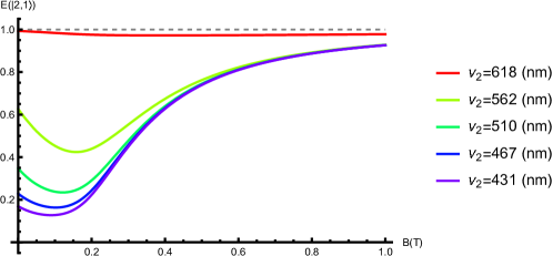
Figure 1: Dependence of the information measure on the parameter $\omega$.

Fig 1. shows the behavior of the measure $E(\left|2,1\right\rangle)$ versus the parameter $\omega$ for the first photon of the wavelength $\nu_{1}=2\pi\kappa_{1}^{-1}=625\ \mathrm{nm}$ and the wavelengths $\nu_{2}=2\pi\kappa_{2}^{-1}$ of the second photon. The magnetic field strength $B$ changes from zero to $1\mathrm{T}$, the momentum projection $np=p_{0}-p_{z}$ is chosen as $2.5\cdot 10^{7\ }\mathrm{\ m}^{-1}$, the electron density is chosen as $\rho=2.6\cdot 10^{20}\mathrm{el\ m}^{-3}$. Note that the entanglement decreases with increasing $\Delta\kappa$ for all the values of $\omega$. We see that turning on of a "weak" magnetic field $B\lesssim 0.1\mathrm{T}$ leads to a decrease of the entanglement, and a further increase of the magnetic field strength leads to the increase of the entanglement.

Fig 2. shows the behavior of the measure $E(\left|2,1\right\rangle)$ on the electron density calculated for the wave length of the first photon $\nu_{1}=2\pi\kappa_{1}^{-1}=625\ \mathrm{nm}$ and for the wave length of the second photon $\nu_{2}=2\pi\kappa_{2}^{-1}=562\ \mathrm{nm}$, whereas the parameter $np$ is equal $2.5\cdot 10^{7\ }\mathrm{\ m}^{-1}$. We see that an increase in density leads to an increase in entanglement. But as the magnetic field increases, the effect of density on entanglement becomes weaker.

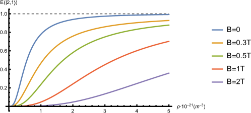
Figure 2: Dependence of the information measure on the electron density for different strengths of the magnetic field.

An increase in the parameter $np$ leads to a sharp decrease in the effect of photon entanglement (see. Fig. 3 for $\nu_{1}=2\pi\kappa_{1}^{-1}=625\ \mathrm{nm}$ and $\nu_{2}=2\pi\kappa_{2}^{-1}=562\ \mathrm{nm}$).

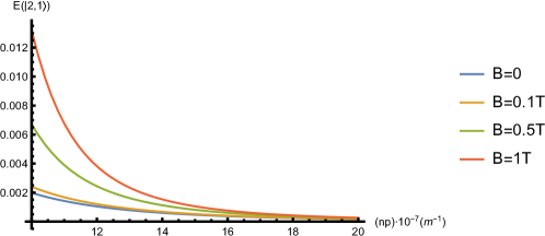
Figure 3: Dependence of the information measure on the parameter $np$.

In the case under consideration the Schmidt measure (57) reads:

$$E_{\mathrm{S}}(\left|2,1\right\rangle)=\frac{1-y^{2}}{2}\sim\epsilon^{4}\Phi\left(2,1\right),\ \ \epsilon\rightarrow 0\,.$$

Numerical calculations for the the Schmidt measure are given almost by the same plot as for the information measure.

Let us consider a state $\left|\Phi_{\mathrm{ph}}\right\rangle$ with two quasi-photons, one of the first kind, and another one of the second kind and with parallel polarizations $\lambda_{1}=1$ and$\ \lambda_{2}=1$. Such a state vector corresponds to $N_{1,1}=N_{2,1}=1$, $N_{1,2}=N_{2,2}=0$ and has the form

$$\left|1,1\right\rangle=C\ \hat{c}_{1,1}^{\dagger}\hat{c}_{2,1}^{\dagger}\left|0\right\rangle\ ,\ \ C=\left\langle 0\right|\hat{c}_{2,1}\hat{c}_{1,1}\hat{c}_{1,1}^{\dagger}\hat{c}_{2,1}^{\dagger}\left|0\right\rangle^{-1/2}\,.$$

One can easily see that in this case, both the information measure of the state $\left|1,1\right\rangle$ are zero $E(\left|1,1\right\rangle)=E_{\mathrm{S}}(\left|1,1\right\rangle)=0$. The same result holds true for the state $\left|2,2\right\rangle=c_{1,2}^{+}c_{2,2}^{+}\left|0\right\rangle$ with two quasi-photons, one of the first kind, and another one of the second kind and with the parallel polarizations $\lambda_{1}=2$,$\ \lambda_{2}=2$, $E(\left|2,2\right\rangle)=E_{\mathrm{S}}(\left|2,2\right\rangle)=0$.

4 Some concluding remarks

A model for describing the QED system consisting of a photon beam interacting with quantized charged spinless media is proposed. The model allows exact analytical analysis which demonstrates that the above system can be reduced to two separate subsystems one related to the charged medium and another one consists of noninteracting quasi-photons. Two versions of the model are considered one without any external field and another one with a constant magnetic field. The charged medium is represented by identical relativistic Bose particles and is characterized by its density and by the energy-momentum of the particles. We believe that the exact solutions of the model could be useful in model descriptions such real physical phenomena as photon entanglement, splitting and fusion of photons (see Ref. [36]) and so on. Using the exact solutions of the model, the problem of photon entanglement is considered. Namely, it is demonstrated that two photons moving in the same direction with different frequencies and with any of two possible linear polarizations, can be in a controlled way entangled by passing through an electron medium without and with applying an external constant magnetic field. We succeeded to express the corresponding entanglement measures (the information and the Schmidt ones) via the parameters characteristic of the problem, such as photon frequencies, magnitude of the magnetic field, and parameters of the electron medium. We have found that, in the general case, the entanglement measures depends on the magnitude of the applied magnetic field and hence can be controlled by the latter. As a rule, the entanglement increases with increasing the magnetic field (with increasing the cyclotron frequency). It should be noted that we did not consider resonance cases where cyclotron frequency approaches photon frequencies. Obviously, the entanglement depends on the parameters that specify the electron medium such as the electron density and electron energy and momentum. We did not study this dependence in detail, these characteristics were fixed by choosing a natural, small parameter in our calculations. The aim of the latter consideration was to demonstrate a possibility for entangling photon beams by the help of an external magnetic field. In contrast with the well-known possibilities of doing this by using crystal devices, the present way allows one to change easily and continuously the entanglement measure.

5 Acknowledgments

The work is supported by Russian Science Foundation, grant No. 19-12-00042.

6 Appendix. Entanglement in two-qubit systems

We recall that a qubit is a two-level quantum-mechanical system with the Hilbert space $\mathcal{H}=\mathbb{C}^{2}$. Vectors in the space $\mathcal{H}$ are two columns $\left|\psi\right\rangle=(\psi_{1},\psi_{2})^{T}$. The scalar product reads: $\langle\psi^{\prime}\left|\psi\right\rangle=\psi_{1}^{\prime\ast}\psi_{1}+\psi_{2}^{\prime\ast}\psi_{2}$. An orthogonal basis $\left|a\right\rangle$, $a=0$, $1$ in $\mathcal{H}$ can be chosen as: $\left|0\right\rangle=(1,0)^{T}$, $\left|1\right\rangle=(0,1)^{T}$, $\langle a\left|a^{\prime}\right\rangle=\delta_{aa^{\prime}}$, $\sum_{a=0,1}\left|a\right\rangle\langle a\mid\ =I$, where $I$ is $2\times 2$ unit matrix.

Examples include the spin of the electron in which the two levels can be taken as spin up and spin down; or the polarization of a single photon in which the two states can be taken to be the vertical polarization and the horizontal polarization.

Let us consider a system, composed of two qubit subsystems $A$ and $B$ with the Hilbert space $\mathcal{H}_{AB}=\mathcal{H}_{A}\otimes\mathcal{H}_{B}$ where $\mathcal{H}_{A}=\mathbb{C}^{2}\$and $\mathcal{H}_{B}=\mathbb{C}^{2}$. The composite system is a four level and is also called the two-qubit system. If $\left|a\right\rangle_{A}$ and $\left|b\right\rangle_{B}$, $a$, $b=0$, $1$, are orthonormal bases in the spaces $\mathcal{H}_{A}$ and $\mathcal{H}_{B}$ respectively, then $\left|\alpha b\right\rangle=\left|a\right\rangle\otimes\left|b\right\rangle$ is a complete and orthonormalized bases in $\mathcal{H}_{AB}$, which is called computational bases,

$$\ \left|\alpha b\right\rangle=\left|a\right\rangle\otimes\left|b\right\rangle=\left(a_{1}b_{1},a_{1}b_{2},a_{2}b_{1},a_{2}b_{2}\right)^{T}\,,$$

$$\ \langle\alpha b\left|\alpha^{\prime}b^{\prime}\right\rangle=\delta_{\alpha\alpha^{\prime}}\delta_{bb^{\prime}}\ ,\ \sum_{\alpha,b=0,1}\left|\alpha b\right\rangle\langle\alpha b\mid\ =\mathbf{I}\,.$$

where $\mathbf{I}$ is $4\times 4$ unit matrix. The vectors of the computational bases are eigenstates of the operator $\sigma_{z}\otimes\sigma_{z}=\mathrm{diag}(1,-1,-1,1)$, namely $\left[\sigma_{z}\otimes\sigma_{z}\right]\left|aa^{\prime}\right\rangle=(-1)^{(a+a^{\prime})}\left|aa^{\prime}\right\rangle$. The basis is often denoted as $\left|\Theta\right\rangle_{s}$,$\ s=1,2,3,4$,

$$\left|\Theta\right\rangle_{1} =\left|00\right\rangle=\left(\begin{array}[c]{cccc}1&0&0&0\end{array}\right)^{T},\ \ \left|\Theta\right\rangle_{2}=\left|01\right\rangle=\left(\begin{array}[c]{cccc}0&1&0&0\end{array}\right)^{T}\ ,$$ (45)

$$\left|\Theta\right\rangle_{3} =\left|10\right\rangle=\left(\begin{array}[c]{cccc}0&0&1&0\end{array}\right)^{T},\ \ \left|\Theta\right\rangle_{4}=\left|11\right\rangle=\left(\begin{array}[c]{cccc}0&0&0&1\end{array}\right)^{T}\,.$$ (48)

A pure state $\left|\Psi\right\rangle_{AB}\in\mathcal{H}_{AB}$ is called separable if and only it can be represented as $\left|\Psi\right\rangle_{AB}=\left|\Psi\right\rangle_{A}\otimes\left|\Psi\right\rangle_{B}$, $\left|\Psi\right\rangle_{A}\in\mathcal{H}_{A}$,$\ \left|\Psi\right\rangle_{B}\in\mathcal{H}_{B}$. Respectively, a state $\left|\Psi\right\rangle_{AB}$ is entangled if it is not separable.

A measure of the entanglement is a real positive number $E(\left|\Psi\right\rangle_{AB})\in\mathbb{R}_{+}$ which is assigned to each state $\left|\Psi\right\rangle_{AB}$. The measure of entanglement is zero for separable states, and assumes its maximum $1$ for maximally entangled states.

An entanglement measure $E(\left|\Psi\right\rangle_{AB})$ of a state $\left|\Psi\right\rangle_{AB}$ of a two-qubit system was proposed by Bennett in Ref. [27]. It reads:

$$E\left(\left|\Psi\right\rangle_{AB}\right)=S\left(\hat{\rho}_{A}\right)=S\left(\hat{\rho}_{B}\right)\ ,$$

$$S\left(\hat{\rho}_{A}\right)=-\mathrm{tr}\left(\hat{\rho}_{A}\log\hat{\rho}_{A}\right),\ \ S\left(\hat{\rho}_{B}\right)=-\mathrm{tr}\left(\hat{\rho}_{B}\log\hat{\rho}_{B}\right)\,,$$ (49)

where $S(\hat{\rho}_{A})$ is von Neumann entropy of a statistical operator $\hat{\rho}_{A}$ of the subsystem $A$, whereas $S(\hat{\rho}_{B})$ is von Neumann entropy of the statistical operator $\hat{\rho}_{B}$ of the subsystem $B$ (one can see that $S(\rho_{A})=S(\rho_{B})$). For a pure state $\left|\Psi\right\rangle_{AB}$, we have:

$$\hat{\rho}_{A}=\mathrm{tr}_{B}\hat{\rho}_{AB}=\sum_{b}\langle b\left|\hat{\rho}_{AB}\mid b\right\rangle\,,$$

$$\hat{\rho}_{B}=\mathrm{tr}_{A}\hat{\rho}_{AB}=\sum_{a}\langle a\left|\hat{\rho}_{AB}\mid a\right\rangle,\quad\hat{\rho}_{AB}=\ _{AB}\mid\Psi\rangle\langle\Psi\mid_{AB}\,.$$

In the case of a pure state, its reduced statistical operators have nonzero quantum entropy, whereas the entropy of the initial pure state is always zero. By definition, a pure state of a two-qubit system is maximally entangled if its reduced statistical operators are proportional to the identity operators.

Let us decompose the state $\left|\Psi\right\rangle_{AB}$ and the operator $\hat{\rho}_{AB}$ in the computational bases,

$$\left|\Psi\right\rangle_{AB}=\sum_{s=1}^{4}\upsilon_{s}\left|\Theta\right\rangle_{s}\Longrightarrow$$

$$\hat{\rho}_{AB}=\left[\upsilon_{1}\left|00\right\rangle+\upsilon_{2}\left|01\right\rangle+\upsilon_{3}\left|10\right\rangle+\upsilon_{4}\left|11\right\rangle\right]\times$$

$$\qquad\quad\left[\upsilon_{1}^{\ast}\langle 00\mid+\upsilon_{2}^{\ast}\langle 01\mid+\upsilon_{3}^{\ast}\langle 10\mid+\upsilon_{4}^{\ast}\langle 11\mid\right]\,.$$

Then, with account taken of the relations

$$\left|0\right\rangle\langle 0\mid\ =\mathrm{diag}\left(1,0\right),\qquad\,\,\,\,\left|1\right\rangle\langle 1\mid\ =\mathrm{diag}\left(0,1\right)\,,$$

$$\left|0\right\rangle\langle 1\mid\ =\mathrm{antidiag}\left(1,0\right),\quad\left|1\right\rangle\langle 0\mid=\mathrm{antidiag}\left(0,1\right)\,,$$

where states $\left|a\right\rangle$ basis vectors in the Hilbert space $\mathcal{H}_{A}$, we obtain:

$$\hat{\rho}_{A}=\ _{B}\langle 0\mid\hat{\rho}_{AB}\left|0\right\rangle_{B}+\ _{B}\langle 1\mid\hat{\rho}_{AB}\left|1\right\rangle_{B}=$$

$$\mid\upsilon_{1}\mid^{2}\left|0\right\rangle\langle 0\mid+\upsilon_{1}\upsilon_{3}^{\ast}\left|0\right\rangle\langle 1\mid+\mid\upsilon_{2}\mid^{2}\left|0\right\rangle\langle 0\mid+\upsilon_{2}\upsilon_{4}^{\ast}\left|0\right\rangle\langle 1\mid$$

$$+\upsilon_{3}\upsilon_{1}^{\ast}\left|1\right\rangle\langle 0\mid+\mid\upsilon_{3}\mid^{2}\left|1\right\rangle\langle 1\mid+\upsilon_{4}\upsilon_{2}^{\ast}\left|1\right\rangle\langle 0\mid+\mid\upsilon_{4}\mid^{2}\left|1\right\rangle\langle 1\mid\ =\left(\begin{array}[c]{ll}\rho_{11}^{\left(A\right)}&\rho_{12}^{\left(A\right)}\\ \rho_{21}^{\left(A\right)}&\rho_{22}^{\left(A\right)}\end{array}\right),$$ (52)

$$\rho_{11}^{\left(A\right)}=\mid\upsilon_{1}\mid^{2}+\mid\upsilon_{2}\mid^{2},\ \rho_{12}^{\left(A\right)}=\upsilon_{1}\upsilon_{3}^{\ast}+\upsilon_{2}\upsilon_{4}^{\ast}\ ,$$

$$\rho_{21}^{\left(A\right)}=\upsilon_{3}\upsilon_{1}^{\ast}+\upsilon_{4}\upsilon_{2}^{\ast},\ \ \rho_{22}^{\left(A\right)}=\mid\upsilon_{3}\mid^{2}+\mid\upsilon_{4}\mid^{2}\,.$$

Calculating the entanglement measure, we can use eigenvalues of the matrix $\hat{\rho}_{A}$,

$$\hat{\rho}^{\left(A\right)}P_{a}=\lambda_{a}P_{a},\ \ \lambda_{a}=\frac{1}{2}\left[\rho_{11}^{\left(A\right)}+\rho_{22}^{\left(A\right)}+\left(-1\right)^{a}y\right],\ a=1,2;$$

$$P_{a}=\left(\begin{array}[c]{c}\frac{\rho_{11}^{\left(A\right)}-\rho_{22}^{\left(A\right)}+\left(-1\right)^{a}y}{2\rho_{21}^{\left(A\right)}}\\ 1\end{array}\right),\ y=\sqrt[+]{\left(\rho_{11}^{\left(A\right)}-\rho_{22}^{\left(A\right)}\right)^{2}+4\left|\rho_{12}^{\left(A\right)}\right|^{2}}$$ (55)

$$=\sqrt{\left(\mid\upsilon_{1}\mid^{2}+\mid\upsilon_{2}\mid^{2}-\mid\upsilon_{4}\mid^{2}-\mid\upsilon_{3}\mid^{2}\right)^{2}+4\left|\upsilon_{1}\upsilon_{3}^{\ast}+\upsilon_{2}\upsilon_{4}^{\ast}\right|^{2}}\,.$$ (56)

Thus, we obtain

$$E\left(\Psi\right)=-\sum_{a=1,2}\lambda_{a}\log_{2}\lambda_{a}=-\left[z\log_{2}z+\left(1-z\right)\log_{2}(1-z)\right],\ \ z=\frac{1+y}{2},$$

and by convention we adopt that $0\log_{2}0\equiv 0$ (see, e.g., Ref. [11]).

It is also known that for a pure two-qubit state one can recognize entanglement by evaluating the so-called Schmidt measure $E_{\mathrm{S}}(\Psi)$, which is the trace of the squared reduced density operators,

$$E_{\mathrm{S}}(\Psi)=1-\mathrm{tr}\left[\left(\hat{\rho}^{(1)}\right)^{2}\right]=1-\sum_{a=1,2}^{2}\lambda_{a}^{2}=$$

$$1-\left[\left(\rho_{11}^{\left(A\right)}\right)^{2}+\left(\rho_{22}^{\left(A\right)}\right)^{2}+2\left|\rho_{12}^{\left(A\right)}\right|^{2}\right]\,.$$ (57)

The Schmidt measure can be considered as an alternative to the information entanglement measure.

References

- [1] F. Bloch and A. Nordsieck, Phys. Rev. 52, 54 (1937)
- [2] N. N. Bogoliubov and D. V. Shirkov, Introduction to the theories to the quantized fields (John Wiley & Sons, New York 1980)
- [3] S. Albeverio, F. Gesztesy, R. Hoegh-Krohn, and H. Holden, Solvable Models in Quantum Mechanics (Springer, Berlin Heidelberg 1988)
- [4] V. G. Bagrov and D. M. Gitman, Exact Solutions of Relativistic Wave Equations (Springer, Dordrecht, 1990)
- [5] E. S. Fradkin, D. M. Gitman, and Sh. M. Shvartsman, Quantum Electrodynam6ics with Unstable Vacuum, (Springer-Verlag, Berlin 1991)
- [6] S.P. Gavrilov and D.M. Gitman, Sov. Phys. Journ. 23, 491 (1980)
- [7] S. Schweber, An Introduction to Relativistic Quantum Field Theory (Harper & Row, New York 1961)
- [8] I.A. Malkin and V.I. Man’ko, Zh. Eksp. Teor. Fiz. 55, 1014(1968)
- [9] J. S. Bell, Speakable and unspeakable in quantum mechanics (Cambridge Univ. Press, New York 1987)
- [10] J. Preskill, Course Information for Physics 219/Computer Science 219, Quantum Computation (Formerly Physics 229), http://theory.caltech.edu/~preskill/ph219/index.html#lecture
- [11] M. A. Nielsen and I.L. Chuang, Quantum computation and quantum information (Cambridge University Press, Cambridge 2000)
- [12] R. Alicki and M. Fannes, Quantum Dynamical Systems (Oxford University Press, New York 2001)
- [13] I. S. Oliveira, et al. NMB Quantum Information Processing, (Elsevier, Amsterdam 2007)
- [14] S. Barz, I. Kassal, M. Ringbauer, Y. O. Lipp, B. Dakic, A. Aspuru-Guzik, and P. Walther, Nature: Scientific Reports 4, 6115, (2014)
- [15] T. Nishioka, Reviews of Modern Physics 90:3, 035007 (2018)
- [16] E. Witten, Reviews of Modern Physics 90:4, 045003 (2018)
- [17] D. Campo and R. Parentani, Phys. Rev. D 72, 045015 (2005)
- [18] S-Y Lin, C-H Chou and B.L. Hu, Phys. Rev. D 81, 084018 (2010)
- [19] J. Adamek, X. Busch and R. Parentani, Phys. Rev. D 87, 124039 (2013)
- [20] X. Busch and R. Parentani, Phys. Rev. D 88, 045023 (2013)
- [21] D E Bruschi, N Friis, I Fuentes and S Weinfurtner, New Journ. Phys. 15, 113016 (2013)
- [22] S. Finazzi, and I. Carusotto, Physical Review A 90(3), 033607 (2014)
- [23] S. P. Gavrilov, D. M. Gitman and A. A. Shishmarev, Phys. Rev. A 91, 052106 (2015)
- [24] A.D. Levin, D.M. Gitman and R.A. Castro, Eur. Phys. J C 74(9), 1 (2014)
- [25] V.G. Bagrov, D.M. Gitman, A.D. Levin, and M. S. Meireles, Intern. Journ. Quantum Information, 15(1), 1750006 (2017)
- [26] D.M. Gitman, A.D. Levin, M. S. Meireles, A.A. Shishmarev, and R.A. Castro, Int. Journ. Mod. Phys. A 33(21), 1850128 (2018)
- [27] C. H. Bennett, H. J. Bernstein, S. Popescu, and B. Schumacher, Phys. Rev. A 53, 2046 (1996)
- [28] W. K. Wootters, Phys. Rev. Lett. 80, 2245 (1998)
- [29] A. Peres, Phys. Rev. Lett. 77, 1413 (1996); M. Horodecki, P. Horodecki, and R. Horodecki, Phys. Lett A 223, 1 (1996)
- [30] K. Życzkowski, P. Horodecki, A. Sanpera, and M. Lewenstein, Phys. Rev. A 58, 883 (1998)
- [31] G. Vidal and R.F. Werner, Phys. Rev. A 65, 032314 (2002)
- [32] V. Vedral, M.B. Plenio, K. Jacobs, and P.L. Knight, Phys. Rev. A 56, 4452 (1997)
- [33] O. Rudolph, Phys. Rev. A 67, 032312 (2003)
- [34] J. Lee, M.S. Kim, Časlav Bruker, Phys. Rev. Lett. 91, 087902 (2003)
- [35] J. Eisert, and H.J. Briegel, Phys. Rev. A 64, 022306 (2001)
- [36] A. I. Smirnov, Izv. Vyssh. Ucheb. Zaved. Fiz. (9) 132 (1974)