The depth of the banana and the impulse stripe illumination for diffuse optical tomography

Abstract.

The stripe illumination lies between the illumination in the spatial-frequency domain and the point illumination. Although the stripe illumination has a periodic structure as the illumination in the spatial-frequency domain, light from the stripe illumination can reach deep regions in biological tissue since it can be regarded as an array of point illuminations. For a pair of a source and a detector, the shape of light paths which connect the source and detector is called the banana shape. First, we investigate the depth of the banana. In the case of the zero boundary condition, we found that the depth of the center of the banana is $d_{\rm SD}/(2\sqrt{2})$, where $d_{\rm SD}$ is the distance between the source and detector on the boundary. In general, the depth is about $0.3d_{\rm SD}$ when $d_{\rm SD}\approx 2\,{\rm cm}$ and the ratio of refractive indices on the boundary is about $1.37$. Next, we perform diffuse optical tomography for the stripe illumination against forward data taken by Monte Carlo simulation. We consider an impulse illumination of the shape of a stripe. This time-resolved measurement is more informative than conventional continuous-wave measurements in the spatial-frequency domain.

1. Introduction

Conventionally in diffuse optical tomography, light has been illuminated and detected with optical fibers. Noncontact diffuse optical tomography can be achieved when a laser beam is sent to a sample to which no optical fiber is attached and the detected light is measured by a CCD or CMOS camera. As an alternative noncontact diffuse optical tomography, measurements in the spatial frequency domain has been proposed (See [1] and references therein).

When the measurement is performed in the spatial frequency domain, the penetration depth of near-infrared light can be controlled by the spatial frequency. Light with high spatial frequencies can reach shallow regions and is reflected back to the surface of the sample. In other words, spatially oscillating light cannot reach deep regions compared with a planar light which uniformly illuminates the surface or a pencil beam which is illuminated at a point on the surface.

In this paper, we consider diffuse optical tomography with the impulse stripe illumination. Since the stripe illumination can be regarded as the illumination with multiple spatial frequencies, on one hand, it is the measurement in the spatial frequency domain. On the other hand, the stripe illumination can be regarded as an array of point illuminations. Hence the stripe illumination acts as a bridge between measurements in the real spatial domain and spatial frequency domain. Moreover, we send an impulse of near-infrared light for the stripe illumination and consider the time-resolved measurement.

For the conventional near-infrared measurement of one point illumination and one point detection, trajectories of the detected light in the sample is known to form a banana shape [2, 3]. This photon-path structure also takes place periodically for the stripe illumination when the outgoing light at dark regions between bright stripes is detected and only light from adjacent bright stripes is dominant in the detected light. In this paper, we consider the shape of the banana. We found that the depth of the center of the banana is about $0.3$ of the source-detector distance for typical measurements for biological tissue.

The remainder of the paper is organized as follows. In Sec. 2, we consider the banana shape for diffuse light. In Sec. 3, the impulse stripe illumination is introduced. In Sec. 4, we obtain tomographic images for the forward data computed by Monte Carlo simulation. Finally, concluding remarks are given in Sec. LABEL:concl.

2. Banana

Let $\boldsymbol{\mathrm{r}}=(\boldsymbol{\mathrm{\rho}},z)$ be a vector in $\mathbb{R}^{3}$, where $\boldsymbol{\mathrm{\rho}}\in\mathbb{R}^{2}$ is a vector in the $x$-$y$ plane. Let $\Omega$ be the half-space ($z>0$):

$$\Omega=\left\{\boldsymbol{\mathrm{r}}\in\mathbb{R}^{3};\;-\infty<x<\infty,\;-\infty<y<\infty,\;0<z<\infty\right\}.$$ (1)

Let $\partial\Omega$ be the boundary of $\Omega$, i.e., the $x$-$y$ plane. Suppose that $\Omega$ is occupied by a medium in which near-infrared light propagates. The outside $\mathbb{R}^{3}\setminus\overline{\Omega}$ is air.

Suppose that light is illuminated at $\boldsymbol{\mathrm{r}}_{s}\in\partial\Omega$ and detected at another point $\boldsymbol{\mathrm{r}}_{d}\in\partial\Omega$. Let $\boldsymbol{\mathrm{r}}_{s}=(x_{s},0,0^{+})^{T}$ and $\boldsymbol{\mathrm{r}}_{d}=(x_{d},0,0)^{T}$ with $-x_{s}=x_{d}=d_{\rm SD}/2>0$, i.e, $d_{\rm SD}$ is the distance between the source and detector. We consider the diffusion equation given by

$$\left\{\begin{aligned} -D_{0}\Delta u+\mu_{a}(\boldsymbol{\mathrm{r}})u=\delta(\boldsymbol{\mathrm{r}}-\boldsymbol{\mathrm{r}}_{s}),&\quad\boldsymbol{\mathrm{r}}\in\Omega,\\ -D_{0}\frac{\partial}{\partial z}u+\frac{1}{\zeta}u=0,&\quad\boldsymbol{\mathrm{r}}\in\partial\Omega,\end{aligned}\right.$$ (2)

where $D_{0}=1/(3\mu_{s}^{\prime})$ with $\mu_{s}^{\prime}$ the reduced scattering coefficient. We assume the diffuse surface reflection and give the constant $\zeta$ by

$$\zeta=2\frac{1+R}{1-R},\quad R=-1.4399\mathfrak{n}^{-2}+0.7099\mathfrak{n}^{-1}+0.6681+0.0636\mathfrak{n},$$ (3)

where $\mathfrak{n}$ is the refractive index of the medium.

To investigate the propagation of the detected light, we assume a point absorber at $\boldsymbol{\mathrm{r}}_{0}=(x_{0},0,z_{0})^{T}$:

$$\mu_{a}(\boldsymbol{\mathrm{r}})=\bar{\mu}_{a}+\eta\delta(\boldsymbol{\mathrm{r}}-\boldsymbol{\mathrm{r}}_{0}),$$ (4)

where $\delta(\cdot)$ is the Dirac delta function, and $\bar{\mu}_{a}>0$, $\eta\geq 0$ are constants. We assume that $\eta$ is small so that the Born approximation (below) holds.

The Green’s function $G(\boldsymbol{\mathrm{r}},\boldsymbol{\mathrm{r}}^{\prime})$ is introduced as

$$\left\{\begin{aligned} -D_{0}\Delta G+\bar{\mu}_{a}G=\delta(\boldsymbol{\mathrm{r}}-\boldsymbol{\mathrm{r}}^{\prime}),&\quad\boldsymbol{\mathrm{r}}\in\Omega,\\ -D_{0}\frac{\partial}{\partial z}G+\frac{1}{\zeta}G=0,&\quad\boldsymbol{\mathrm{r}}\in\partial\Omega.\end{aligned}\right.$$ (5)

Thus, the following identity is derived.

$$u(\boldsymbol{\mathrm{r}};\boldsymbol{\mathrm{r}}_{0},\boldsymbol{\mathrm{r}}_{s})=G(\boldsymbol{\mathrm{r}},\boldsymbol{\mathrm{r}}_{s})-\eta G(\boldsymbol{\mathrm{r}},\boldsymbol{\mathrm{r}}_{0})u(\boldsymbol{\mathrm{r}}_{0})$$ (6)

With the Born approximation, we have $u\approx u_{B}$, where

$$u_{B}(\boldsymbol{\mathrm{r}};\boldsymbol{\mathrm{r}}_{0},\boldsymbol{\mathrm{r}}_{s})=G(\boldsymbol{\mathrm{r}},\boldsymbol{\mathrm{r}}_{s})-\eta G(\boldsymbol{\mathrm{r}},\boldsymbol{\mathrm{r}}_{0})G(\boldsymbol{\mathrm{r}}_{0},\boldsymbol{\mathrm{r}}_{s})$$ (7)

We have (see Appendix A)

$$G(\boldsymbol{\mathrm{r}}_{0},\boldsymbol{\mathrm{r}}_{s}) =\frac{z_{e}}{2\pi D_{0}}\int_{0}^{\infty}qJ_{0}(q|x_{0}-x_{s}|)\frac{e^{-\lambda(q)z_{0}}}{1+\lambda(q)z_{e}}\,dq,$$ (8)

$$G(\boldsymbol{\mathrm{r}}_{0},\boldsymbol{\mathrm{r}}_{d}) =\frac{z_{e}}{2\pi D_{0}}\int_{0}^{\infty}qJ_{0}(q|x_{0}-x_{d}|)\frac{e^{-\lambda(q)z_{0}}}{1+\lambda(q)z_{e}}\,dq,$$

where

$$\lambda(q)=\sqrt{\frac{\mu_{a}}{D_{0}}+q^{2}},\quad z_{e}=\zeta D_{0}.$$ (9)

Since

$$\frac{\partial}{\partial z_{0}}u_{B}(\boldsymbol{\mathrm{r}}_{d};\boldsymbol{\mathrm{r}}_{0},\boldsymbol{\mathrm{r}}_{s})$$ (10)

$$=-\eta\left[\frac{\partial G(\boldsymbol{\mathrm{r}}_{d},\boldsymbol{\mathrm{r}}_{0})}{\partial z_{0}}G(\boldsymbol{\mathrm{r}}_{0},\boldsymbol{\mathrm{r}}_{s})+G(\boldsymbol{\mathrm{r}}_{d},\boldsymbol{\mathrm{r}}_{0})\frac{\partial G(\boldsymbol{\mathrm{r}}_{0},\boldsymbol{\mathrm{r}}_{s})}{\partial z_{0}}\right],$$

we obtain

$$\frac{\partial}{\partial z_{0}}u_{B}(\boldsymbol{\mathrm{r}}_{d};\boldsymbol{\mathrm{r}}_{0},\boldsymbol{\mathrm{r}}_{s})=\eta\left(\frac{z_{e}}{2\pi D_{0}}\right)^{2}$$ (11)

$$\times\Biggl{[}\left(\int_{0}^{\infty}qJ_{0}(q|x_{0}-x_{d}|)\frac{\lambda(q)e^{-\lambda(q)z_{0}}}{1+\lambda(q)z_{e}}\,dq\right)$$

$$\times\left(\int_{0}^{\infty}qJ_{0}(q|x_{0}-x_{s}|)\frac{e^{-\lambda(q)z_{0}}}{1+\lambda(q)z_{e}}\,dq\right)$$

$$+\left(\int_{0}^{\infty}qJ_{0}(q|x_{0}-x_{d}|)\frac{e^{-\lambda(q)z_{0}}}{1+\lambda(q)z_{e}}\,dq\right)$$

$$\times\left(\int_{0}^{\infty}qJ_{0}(q|x_{0}-x_{s}|)\frac{\lambda(q)e^{-\lambda(q)z_{0}}}{1+\lambda(q)z_{e}}\,dq\right)\Biggr{]}.$$

Let us investigate the position of the center of the banana shape by moving the point absorber. First let us consider the case of $\eta=0$. The reciprocal property $G(\boldsymbol{\mathrm{r}},\boldsymbol{\mathrm{r}}^{\prime})=G(\boldsymbol{\mathrm{r}}^{\prime},\boldsymbol{\mathrm{r}})$ of the Green’s function implies that the banana is symmetric about $\boldsymbol{\mathrm{r}}_{s}$ and $\boldsymbol{\mathrm{r}}_{d}$. Hence, hereafter we will set $x_{0}=0$.

Suppose $\eta$ is positive. If the point absorber is placed at the center of the banana, the detected light $u(\boldsymbol{\mathrm{r}}_{d};\boldsymbol{\mathrm{r}}_{0},\boldsymbol{\mathrm{r}}_{s})$ should take the minimum value. In this case, we have $\frac{\partial}{\partial z_{0}}u_{B}(\boldsymbol{\mathrm{r}}_{d};\boldsymbol{\mathrm{r}}_{0},\boldsymbol{\mathrm{r}}_{s})=0$. The condition implies

$$\int_{0}^{\infty}qJ_{0}\left(\frac{qd_{\rm SD}}{2}\right)\frac{\lambda(q)e^{-\lambda(q)z_{0}}}{1+\lambda(q)z_{e}}\,dq=0.$$ (12)

By using $qdq=\lambda d\lambda$ and putting $x=\lambda d_{\rm SD}/2$, we have

$$\int_{\sqrt{\frac{\mu_{a}}{D_{0}}}}^{\infty}J_{0}\left(\frac{d_{\rm SD}}{2}\sqrt{\lambda^{2}-\frac{\mu_{a}}{D_{0}}}\right)\frac{\lambda^{2}e^{-\lambda z_{0}}}{1+\lambda z_{e}}\,d\lambda$$ (13)

$$=\left(\frac{2}{d_{\rm SD}}\right)^{3}\int_{a}^{\infty}J_{0}\left(\sqrt{x^{2}-a^{2}}\right)\frac{x^{2}e^{-wx}}{1+bx}\,dx$$

$$=0,$$

where

$$a=\frac{d_{\rm SD}}{2}\sqrt{\frac{\bar{\mu}_{a}}{D_{0}}},\quad b=\frac{2z_{e}}{d_{\rm SD}},\quad w=\frac{2z_{0}}{d_{\rm SD}}.$$ (14)

Thus the problem reduces to the problem of finding the zero of the following function $\Lambda(w)$:

$$\Lambda(w;a,b)=\int_{a}^{\infty}J_{0}\left(\sqrt{x^{2}-a^{2}}\right)\frac{x^{2}e^{-wx}}{1+bx}\,dx.$$ (15)

Assuming $\bar{\mu}_{a}$ is small, let us set $a=0$. For large $w$,

$$\Lambda(w;0,b)=\int_{0}^{\infty}J_{0}(x)\frac{x^{2}e^{-wx}}{1+bx}\,dx\approx\int_{0}^{\infty}x^{2}e^{-wx}\,dx=\frac{2}{w^{3}}.$$ (16)

When $w=0$, we have

$$\Lambda(0;0,b) =\int_{0}^{\infty}J_{0}(x)\frac{x^{2}}{1+bx}\,dx$$ (17)

$$=\frac{1}{b}\int_{0}^{\infty}J_{0}(x)x\,dx-\frac{1}{b}\int_{0}^{\infty}J_{0}(x)\frac{x}{1+bx}\,dx$$

$$=-\frac{1}{b^{3}}\int_{0}^{\infty}J_{0}(t/b)\frac{t}{1+t}\,dt$$

$$=-\frac{1}{b^{2}}+\frac{\pi}{2b^{3}}\left(H_{0}\left(\frac{1}{b}\right)-Y_{0}\left(\frac{1}{b}\right)\right)<0,$$

where we used the Hankel transform $\int_{0}^{\infty}J_{0}(qx)x\,dx=\delta(q)/q$. Here, the Struve function $H_{0}$ and Bessel function of the second kind $Y_{0}$ are given by

$$H_{0}(x) =\frac{1}{\sqrt{\pi}}\sum_{n=0}^{\infty}\frac{(-1)^{n}x^{2n+1}}{[(2n+1)!!]2^{n}\Gamma(n+3/2)},$$ (18)

$$Y_{0}(x) =\frac{1}{\pi}\left.\left(\frac{\partial J_{\nu}(x)}{\partial\nu}-\frac{\partial J_{-\nu}(x)}{\partial\nu}\right)\right|_{\nu=0}$$

$$=\frac{2}{\pi}J_{0}(x)\ln\frac{x}{2}-\frac{2}{\pi}\sum_{n=0}^{\infty}\frac{(-1)^{n}}{(n!)^{2}}\left(\frac{x}{2}\right)^{2n}\psi(n+1),$$

where $\psi$ is the digamma function. The facts that $\Lambda(w;0,b)$ is positive for large $w$ and negative for small $w>0$ imply that $\Lambda(w;0,b)$ has a zero.

In the case of $b=0$ (i.e., the zero boundary condition $z_{e}=0$), we obtain

$$\Lambda(w;0,0)=\int_{0}^{\infty}J_{0}(x)x^{2}e^{-wx}\,dx=\frac{\sqrt{w^{2}+1}(2w^{2}-1)}{(1+w^{2})^{3}}.$$ (19)

The function $\Lambda(w;0,0)$ is plotted in Fig. 1. Hence in this case $\Lambda(w;0,0)$ becomes zero at

$$w=\frac{1}{\sqrt{2}}\approx 0.7$$ (20)

That is,

$$z_{0}=\frac{d_{\rm SD}}{2\sqrt{2}}\approx 0.35d_{\rm SD}.$$ (21)

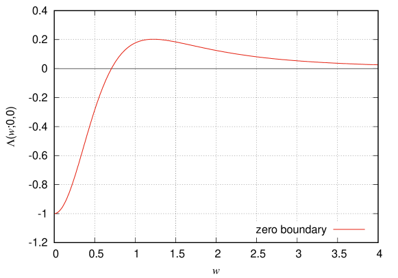
Figure 1. The function $\Lambda(w;0,0)$ in (19) is plotted.

In general for nonzero $b>0$ (i.e., the Robin boundary condition $z_{e}>0$), $\Lambda(w;0,b)$ is numerically obtained as shown in Figs. 2 and 3. For example, for $\mathfrak{n}=1.33$, the zero of $\Lambda(w;0,b)$ is about $w=0.61$ for $d_{\rm SD}=30\,{\rm mm}$. In this case, $z_{0}=9\,{\rm mm}$, i.e., $z_{0}/d_{\rm SD}=0.3$. Moreover, the zero of $\Lambda(w;0,b)$ is about $w=0.60$ for $d_{\rm SD}=30\,{\rm mm}$ and $\mathfrak{n}=1.37$. In this case, $z_{0}=9\,{\rm mm}$ ($z_{0}/d_{\rm SD}=0.3$). For $d_{\rm SD}=20\,{\rm mm}$ and $\mathfrak{n}=1.37$, the zero of $\Lambda(w;0,b)$ is about $w=0.56$, which results in $z_{0}=5.6\,{\rm mm}$ ($z_{0}/d_{\rm SD}=0.28$).

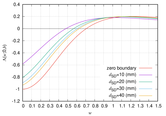
Figure 2. The function $\Lambda(w;0,b)$ ($b=2z_{e}/d_{\rm SD}$) is plotted for different $d_{\rm SD}$ for $\mathfrak{n}=1.33$, $D_{0}=1/3$ ($\mu_{s}^{\prime}=1\,{\rm mm}$).

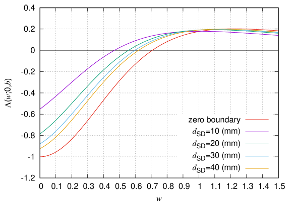
Figure 3. The function $\Lambda(w;0,b)$ ($b=2z_{e}/d_{\rm SD}$) is plotted for different $d_{\rm SD}$ for $\mathfrak{n}=1.37$, $D_{0}=1/3$ ($\mu_{s}^{\prime}=1\,{\rm mm}$).

3. Impulse stripe illumination

Let $c_{0}$ be the speed of light in vacuum. Then $c=c_{0}/\mathfrak{n}$ is the speed of light in the medium. Let $T>0$ be the observation time. The diffuse fluence rate $u(\boldsymbol{\mathrm{r}},t)$ for the impulse illumination obeys the following diffusion equation.

$$\left\{\begin{aligned} \frac{1}{c}\frac{\partial}{\partial t}u-D_{0}\Delta u+\mu_{a}(\boldsymbol{\mathrm{r}})u=f,&\quad(x,t)\in\Omega\times(0,T),\\ -D_{0}\frac{\partial}{\partial z}u+\frac{1}{\zeta}u=0,&\quad(x,t)\in\partial\Omega\times(0,T),\\ u=0,&\quad\boldsymbol{\mathrm{r}}\in\Omega,\quad t=0,\end{aligned}\right.$$ (22)

where $f(\boldsymbol{\mathrm{r}},t)$ is the incident beam. The source term $f(\boldsymbol{\mathrm{r}},t)$ is given by

$$f(\boldsymbol{\mathrm{r}},t)=f_{0}a(\boldsymbol{\mathrm{\rho}})\delta(t)\delta(z),$$ (23)

where $f_{0}>0$ is a constant which is determined by the beam. Let $L,\ell$ be the pitch and scan step, respectively. The function $a(\boldsymbol{\mathrm{\rho}})$ is given by

$$a(\boldsymbol{\mathrm{\rho}})=a_{n}(\boldsymbol{\mathrm{\rho}})=\sum_{j=-\infty}^{\infty}\delta\left(x-jL-\frac{2n-1}{2}\ell\right),$$ (24)

where $n=1,\dots,N_{f}$ and $N_{f}$ is the number of scans. For illumination, we set

$$L=32\,{\rm mm},\quad\ell=2\,{\rm mm},\quad N_{f}=16.$$ (25)

We define

$$p_{l}=\frac{2\pi l}{L},\quad l\in\mathbb{Z}.$$ (26)

Then the function $a_{n}(\boldsymbol{\mathrm{\rho}})$ can be written as

$$a_{n}(\boldsymbol{\mathrm{\rho}})=\frac{1}{L}\sum_{l=-\infty}^{\infty}e^{ip_{l}x}e^{-ip_{l}(2n-1)\ell/2},$$ (27)

where we used the Poisson sum formula,

$$\sum_{j=-\infty}^{\infty}\delta(x-2\pi j)=\frac{1}{2\pi}\sum_{l=-\infty}^{\infty}e^{ilx}.$$ (28)

The expression (27) implies that the solution to (22) can be expressed as

$$u(\boldsymbol{\mathrm{r}},t)=\sum_{l=-\infty}^{\infty}u_{l}(\boldsymbol{\mathrm{r}},t),$$ (29)

where $u_{l}$ ($l=-\infty,\dots,\infty$) is the solution of (22) for

$$f(\boldsymbol{\mathrm{r}},t)=f_{l}(\boldsymbol{\mathrm{r}},t)=\frac{f_{0}}{L}e^{ip_{l}x}e^{-ip_{l}(2n-1)\ell/2}\delta(t)\delta(z).$$ (30)

For constant $\mu_{a}$, it is known that the penetration depth (i.e., the decay rate of $u(\boldsymbol{\mathrm{r}})$ in the $z$-direction) depends on the spatial frequency $p_{l}$. We have asymptotically [1, 4]

$$u_{l}(\boldsymbol{\mathrm{r}},t)\sim\mbox{const.}\times e^{-z\sqrt{\mu_{\rm eff}^{2}+p_{l}^{2}}},$$ (31)

where

$$\mu_{\rm eff}=\sqrt{3\mu_{a}(\mu_{a}+\mu_{s}^{\prime})}.$$ (32)

Since $u$ is given by the sum of $u_{l}$ in (29), the diffuse light $u$ penetrates deeper than the light by a single sinusoidal illumination.

Next, we consider the relation between the pitch $L$ and the penetration depth. The outgoing light is detected at $\boldsymbol{\mathrm{r}}_{d}^{(m,n)}={{}^{t}}(x_{d}^{(m,n)},y,0)$, where $y\in\mathbb{R}$ and

$$x_{d}^{(m,n)}=\frac{2m-1}{2}L+(n-1)\ell\quad(m=1,\dots,N_{d})$$ (33)

for each $n=1,\dots,N_{f}$. For each $n$, light is detected at $N_{d}$ points. In total, light is measured at $N_{d}N_{f}$ points in the $x$-axis. We set

$$N_{d}=3.$$ (34)

Let us consider the separation between the source at $(2n-1)\ell/2$ and $x_{d}^{(1,n)}$. This distance $d_{\rm SD}$ is given by

$$d_{\rm SD}=\frac{L-\ell}{2}=15\,{\rm mm},$$ (35)

where we put $L=32\,{\rm mm}$ and $\ell=2\,{\rm mm}$. Assuming the relation $z_{0}\approx 0.3d_{\rm SD}$, we find that the depth of the banana is

$$z_{0}\approx 4.5\,{\rm mm}.$$ (36)

The above formula $d_{\rm SD}=(L-\ell)/2$ implies that the information at a deep tissue can be extracted with large $L$.

4. Diffuse optical tomography

In our numerical experiment by Monte Carlo simulation, an absorber bar ($\mu_{a}=0.02\,{\rm mm}^{-1}$, $\mu_{s}=10\,{\rm mm}^{-1}$, ${\rm g}=0.9$) is embedded along the $y$-axis. Here, $\mu_{s}$ is the scattering coefficient, ${\rm g}$ is the scattering asymmetry parameter, and $\mu_{s}^{\prime}=(1-{\rm g})\mu_{s}$. In the $x$-$z$ plane, the positions of four corners of the absorber rectangle are $(58,4)$, $(58,10)$, $(64,4)$, and $(64,10)$ in the unit of ${\rm mm}$. The Monte Carlo simulation was performed in a box ($0\leq x\leq 128\,{\rm mm}$, $0\leq y\leq 128\,{\rm mm}$, $0\leq z\leq 40\,{\rm mm}$) with voxel size $2\,{\rm mm}\,\times\,2\,{\rm mm}\,\times\,2\,{\rm mm}$. The Robin boundary condition is considered on the illumination plane (i.e., according to the Fresnel reflection a part of outgoing photons reenters the medium instead of exiting it). The zero boundary condition is imposed on other boundaries. The cross section of the absorber is a square on a side of $6\,{\rm mm}$. In the depth direction along the $z$-axis, the absorber rod exists in $4\,{\rm mm}\leq z\leq 10\,{\rm mm}$. In the medium, we set

$$\bar{\mu}_{a}=0.01\,{\rm mm}^{-1},\quad\mu_{s}^{\prime}=1\,{\rm mm}^{-1},\quad\mathfrak{n}=1.4.$$ (37)

Let us extend the interval $(0,T)$ to $(-\infty,\infty)$ by the limit $T\to\infty$ and zero extension for $t<0$, we consider the Fourier transform as

$$v^{n}(\boldsymbol{\mathrm{r}},\omega)=\int_{-\infty}^{\infty}e^{-i\omega t}u(\boldsymbol{\mathrm{r}},t)\,dt$$ (38)

for $n=1,\dots,N_{f}$.

We write the absorption coefficient $\mu_{a}(\boldsymbol{\mathrm{r}})$ as

$$\mu_{a}(\boldsymbol{\mathrm{r}})=\bar{\mu}_{a}+\delta\mu_{a}(\boldsymbol{\mathrm{r}})\ ,$$ (39)

where $\bar{\mu}_{a}$ is a positive constant and $\left.\mu_{a}\right|_{\partial\Omega}=\bar{\mu}_{a}$. We have

$$\left\{\begin{aligned} -D_{0}\Delta v^{n}+\left(\alpha(\omega)+\delta\mu_{a}(\boldsymbol{\mathrm{r}})\right)v^{n}=f_{0}a_{n}(\boldsymbol{\mathrm{\rho}})\delta(z),&\quad x\in\Omega,\\ -D_{0}\frac{\partial}{\partial z}v^{n}+\frac{1}{\zeta}v^{n}=0,&\quad x\in\partial\Omega,\end{aligned}\right.$$ (40)

where

$$\alpha(\omega)=\bar{\mu}_{a}+\frac{i\omega}{c}.$$ (41)

Let us consider the Green’s function $G_{\omega}(\boldsymbol{\mathrm{r}},\boldsymbol{\mathrm{r}}^{\prime})$ for (40), which satisfies

$$\left\{\begin{aligned} -D_{0}\Delta G_{\omega}+\alpha(\omega)G_{\omega}=\delta(\boldsymbol{\mathrm{r}}-\boldsymbol{\mathrm{r}}^{\prime}),&\quad x\in\Omega,\\ -D_{0}\frac{\partial}{\partial z}G_{\omega}+\frac{1}{\zeta}G_{\omega}=0,&\quad x\in\partial\Omega.\end{aligned}\right.$$ (42)

We obtain

$$G_{\omega}(\boldsymbol{\mathrm{r}},\boldsymbol{\mathrm{r}}^{\prime}) =\frac{1}{(2\pi)^{2}}\int_{\mathbb{R}^{2}}e^{i\boldsymbol{\mathrm{q}}\cdot(\boldsymbol{\mathrm{\rho}}-\boldsymbol{\mathrm{\rho}}^{\prime})}H_{\omega}(|\boldsymbol{\mathrm{q}}|,z,z^{\prime})\,d\boldsymbol{\mathrm{q}},$$ (43)

where

$$Q_{\omega}(q)=\sqrt{\frac{\alpha(\omega)}{D_{0}}+q^{2}},$$ (44)

and

$$H_{\omega}(q,z,z^{\prime})=\frac{1}{2D_{0}Q_{\omega}(q)}$$ (45)

$$\times\left[e^{-Q_{\omega}(q)|z-z^{\prime}|}-\frac{1-Q_{\omega}(q)z_{e}}{1+Q_{\omega}(q)z_{e}}e^{-Q_{\omega}(q)|z+z^{\prime}|}\right].$$

Let $v_{0}^{n}$ be the solution of the diffusion equation in (40) for which $\delta\mu_{a}$ is removed. We have

$$v_{0}^{n}(\boldsymbol{\mathrm{r}},\omega) =f_{0}\sum_{j=-\infty}^{\infty}\int_{-\infty}^{\infty}G_{\omega}\left(\boldsymbol{\mathrm{r}};jL+\frac{2n-1}{2}\ell,y^{\prime},0\right)\,dy^{\prime}$$ (46)

$$=\frac{f_{0}}{L}\sum_{l=-\infty}^{\infty}H_{\omega}(p_{l},z,0)e^{ip_{l}x}e^{-ip_{l}(2n-1)\ell/2}$$

$$=v_{0}^{n}(x,z,\omega),$$

where the Green’s function was expressed as $G_{\omega}(\boldsymbol{\mathrm{r}},\boldsymbol{\mathrm{r}}^{\prime})=G_{\omega}(\boldsymbol{\mathrm{r}};x^{\prime},y^{\prime},z^{\prime})$.

Within the diffusion approximation we have

$$\ln{\frac{v_{0}^{n}(\boldsymbol{\mathrm{r}}_{d}^{(j)},\omega)}{v^{n}(\boldsymbol{\mathrm{r}}_{d}^{(j)},\omega)}}\approx\ln{\frac{I_{0}^{n}(\boldsymbol{\mathrm{r}}_{d}^{(j)},-\boldsymbol{\hat{\mathrm{z}}},\omega)}{I^{n}(\boldsymbol{\mathrm{r}}_{d}^{(j)},-\boldsymbol{\hat{\mathrm{z}}},\omega)}},$$ (47)

where $\boldsymbol{\hat{\mathrm{z}}}={{}^{t}}(0,0,1)$. Here, $I_{0}^{n}(\boldsymbol{\mathrm{r}}_{d}^{(j)},-\boldsymbol{\hat{\mathrm{z}}},\omega)$ and $I^{n}(\boldsymbol{\mathrm{r}}_{d}^{(j)},-\boldsymbol{\hat{\mathrm{z}}},\omega)$ are Fourier transforms of specific intensities in the outer normal direction at $\boldsymbol{\mathrm{r}}_{d}^{(j)}$ for $\mu_{a}=\bar{\mu}_{a}$ and $\mu_{a}=\bar{\mu}_{a}+\delta\mu_{a}$ with the $n$th scan.

We will discretize $\omega$ as

$$\omega_{k}=k\Delta\omega,\quad k=1,\dots,N_{\omega},$$ (48)

where $N_{\omega}$ is the number of points for $\omega$.

We note that

$$\int_{-\infty}^{\infty}G_{\omega}(\boldsymbol{\mathrm{r}},\boldsymbol{\mathrm{r}}^{\prime})\,dy^{\prime}$$ (49)

$$=\frac{1}{2\pi}\int_{-\infty}^{\infty}e^{iq(x-x^{\prime})}\frac{1}{2D_{0}Q_{\omega}(q)}$$

$$\times\left[e^{-Q_{\omega}(q)|z-z^{\prime}|}-\frac{1-Q_{\omega}(q)z_{e}}{1+Q_{\omega}(q)z_{e}}e^{\ -Q_{\omega}(q)|z+z^{\prime}|}\right]\,dq$$

$$=\frac{1}{\pi}\int_{0}^{\infty}\cos[q(x-x^{\prime})]\frac{1}{2D_{0}Q_{\omega}(q)}$$

$$\times\left[e^{-Q_{\omega}(q)|z-z^{\prime}|}-\frac{1-Q_{\omega}(q)z_{e}}{1+Q_{\omega}(q)z_{e}}e^{\ -Q_{\omega}(q)|z+z^{\prime}|}\right]\,dq$$

$$=H_{\omega}(x-x^{\prime},z,z^{\prime}).$$

The numerical computation of $H_{\omega}$ is described in Appendix B.

We define

$$\psi^{n}(x_{d}^{(m,n)},\omega)=\ln{\frac{\left\langle I_{0}^{n}(\boldsymbol{\mathrm{r}}_{d}^{(m,n)},-\boldsymbol{\hat{\mathrm{z}}},\omega)\right\rangle}{\left\langle I^{n}(\boldsymbol{\mathrm{r}}_{d}^{(m,n)},-\boldsymbol{\hat{\mathrm{z}}},\omega)\right\rangle}},$$ (50)

where $\langle\cdot\rangle$ denotes the average over $y$.

Since $\delta\mu_{a}$ does not depend on $y$, we write

$$\delta\mu_{a}(\boldsymbol{\mathrm{r}})=\eta(x,z).$$ (51)

We note the identity:

$$v^{n}(\boldsymbol{\mathrm{r}},\omega)=v_{0}^{n}(\boldsymbol{\mathrm{r}},\omega)-\int_{\Omega}G_{\omega}(\boldsymbol{\mathrm{r}},\boldsymbol{\mathrm{r}}^{\prime})\delta\mu_{a}(\boldsymbol{\mathrm{r}}^{\prime})v^{n}(\boldsymbol{\mathrm{r}}^{\prime},\omega)\,d\boldsymbol{\mathrm{r}}^{\prime}.$$ (52)

Since $v_{0}^{n}$ is independent of $y$, the above identity implies $v^{n}(\boldsymbol{\mathrm{r}},\omega)=v^{n}(x,z,\omega)$ is also independent of $y$. We have

$$v^{n}(x,z,\omega)=v_{0}^{n}(x,z,\omega)$$ (53)

$$-\int_{0}^{\infty}\int_{-\infty}^{\infty}H_{\omega}(x-x^{\prime},z,z^{\prime})\eta(x^{\prime},z^{\prime})v^{n}(x^{\prime},z^{\prime},\omega)\,dx^{\prime}dz^{\prime}.$$

By the (first) Born approximation,

$$v^{n}\approx v_{0}^{n}+v_{1}^{n},$$ (54)

where

$$v_{1}^{n}(x,z,\omega) =-\int_{0}^{\infty}\int_{-\infty}^{\infty}v_{0}^{n}(x^{\prime},z^{\prime},\omega)$$ (55)

$$\times H_{\omega}(x-x^{\prime},z,z^{\prime})\eta(x^{\prime},z^{\prime})\,dx^{\prime}dz^{\prime}.$$

Let us write

$$\left(K_{1}\eta\right)(x,\omega)=-v_{1}^{n}(x,0,\omega),$$ (56)

and introduce operator $\check{K}_{1}$ as

$$\left(\check{K}_{1}\eta\right)(x,\omega)=\frac{1}{v_{0}^{n}(x,0,\omega)}\left(K_{1}\eta\right)(x,\omega).$$ (57)

For boundary values of $v^{n},v_{0}^{n}$, we note that

$$\psi=\psi^{n}(x,\omega)=\ln\frac{v_{0}^{n}(x,0,\omega)}{v^{n}(x,0,\omega)}.$$ (58)

Let us consider the Rytov approximation:

$$\psi\approx\psi_{R}=-\frac{v_{1}^{n}}{v_{0}^{n}}.$$ (59)

We introduce the forward operator $J$ such that

$$\psi_{R}=J\eta.$$ (60)

We have

$$\left(J\eta\right)(x,\omega)=\left(\check{K}_{1}\eta\right)(x,\omega)$$ (61)

$$=\frac{1}{v_{0}^{n}(x,0,\omega)}\int_{0}^{\infty}\int_{-\infty}^{\infty}H_{\omega}(x-x^{\prime},0,z^{\prime})$$

$$\times v_{0}^{n}(x^{\prime},z^{\prime},\omega)\eta(x^{\prime},z^{\prime})\,dx^{\prime}dz^{\prime}.$$

Let us write

$$\eta\approx\mathcal{J}\psi,$$ (62)

where

$$\mathcal{J}=J_{\rm reg}^{+}.$$ (63)

Here, $J_{\rm reg}^{+}$ is the regularized pseudoinverse of $J$.

We set

$$\nu_{1}=m+(n-1)N_{d},$$ (64)

where

$$1\leq m\leq N_{d},\quad 1\leq n\leq N_{f}.$$ (65)

We can introduce vector $\boldsymbol{\mathrm{\psi}}$ as

$$\{\boldsymbol{\mathrm{\psi}}(\omega_{k})\}_{\nu_{1}}=\psi^{n}(x_{d}^{(m,n)},\omega_{k}),\quad 1\leq\nu_{1}\leq N_{f}N_{d}=N_{\nu_{1}},$$ (66)

where $k=1,\dots,N_{\omega}$.

Suppose that in the medium the inhomogeneity exists in the region $[x_{\rm min},x_{\rm max}]\times[z_{\rm min},z_{\rm max}]$, where $x_{\rm min},x_{\rm max}$ ($x_{\rm min}<x_{\rm max}$), and $z_{\rm min},z_{\rm max}$ ($0<z_{\rm min}<z_{\rm max}$) are constants. We discretize $x,z$ as

$$x_{j_{1}}=(j_{1}-1)\Delta x+x_{\rm min}\quad(j_{1}=1,\dots,N_{x}),\quad\Delta x=\frac{x_{\rm max}-x_{\rm min}}{N_{x}-1},$$ (67)

$$z_{j_{2}}=(j_{2}-1)\Delta z+z_{\rm min}\quad(j_{2}=1,\dots,N_{z}),\quad\Delta z=\frac{z_{\rm max}-z_{\rm min}}{N_{z}-1}.$$

We set

$$\nu_{2}=j_{1}+(j_{2}-1)N_{x},$$ (68)

where

$$1\leq j_{1}\leq N_{x},\quad 1\leq j_{2}\leq N_{z}.$$ (69)

We define $\boldsymbol{\mathrm{K}}_{0}(\omega_{k})\in\mathbb{C}^{N_{\nu_{1}}+NxNz}$, $1\leq k\leq N_{\omega}$, as

$$\{\boldsymbol{\mathrm{K}}_{0}(\omega_{k})\}_{\nu_{1}} =-v_{0}^{n}(x_{d}^{(m,n)},0,\omega_{k}),$$ (70)

$$\{\boldsymbol{\mathrm{K}}_{0}(\omega_{k})\}_{N_{\nu_{1}}+\nu_{2}} =-v_{0}^{n}(x_{j_{1}},z_{j_{2}},\omega_{k}).$$

For given a vector $\boldsymbol{\mathrm{b}}\in\mathbb{R}^{N_{x}N_{z}}$, we define

$$\boldsymbol{\mathrm{K}}_{1}(\omega_{k};\boldsymbol{\mathrm{b}})\in\mathbb{C}^{N_{\nu_{1}}+N_{x}N_{z}},\quad 1\leq k\leq N_{\omega},$$ (71)

as

$$\{\boldsymbol{\mathrm{K}}_{1}(\omega_{k};\boldsymbol{\mathrm{b}})\}_{\nu_{1}}=-\sum_{j_{1}^{\prime}=1}^{N_{x}}\sum_{j_{2}^{\prime}=1}^{N_{z}}H_{\omega_{k}}\left(x_{d}^{(m,n)}-x_{j_{1}^{\prime}},0,z_{j_{2}^{\prime}}\right)$$ (72)

$$\times\{\boldsymbol{\mathrm{b}}\}_{\nu_{2}^{\prime}}\{\boldsymbol{\mathrm{K}}_{0}(\omega_{k})\}_{N_{\nu_{1}}+\nu_{2}^{\prime}}\,\Delta x\Delta z,$$

$$\{\boldsymbol{\mathrm{K}}_{1}(\omega_{k};\boldsymbol{\mathrm{b}})\}_{N_{\nu_{1}}+\nu_{2}}=-\sum_{j_{1}^{\prime}=1}^{N_{x}}\sum_{j_{2}^{\prime}=1}^{N_{z}}H_{\omega_{k}}\left(x_{j_{1}}-x_{j_{1}^{\prime}},z_{j_{2}},z_{j_{2}^{\prime}}\right)$$ (73)

$$\times\{\boldsymbol{\mathrm{b}}\}_{\nu_{2}^{\prime}}\{\boldsymbol{\mathrm{K}}_{0}(\omega_{k})\}_{N_{\nu_{1}}+\nu_{2}^{\prime}}\,\Delta x\Delta z,$$

where $\nu_{2}=j_{1}+(j_{2}-1)N_{x}$, $\nu_{2}^{\prime}=j_{1}^{\prime}+(j_{2}^{\prime}-1)N_{x}$. We note that

$$v_{1}^{n}\left(x_{d}^{(m,n)},0,\omega\right) =-\left\{\boldsymbol{\mathrm{K}}_{1}(\omega;\boldsymbol{\mathrm{\eta}})\right\}_{\nu_{1}},$$ (74)

$$v_{1}^{n}\left(x_{j_{1}},z_{j_{2}},\omega\right) =-\left\{\boldsymbol{\mathrm{K}}_{1}(\omega;\boldsymbol{\mathrm{\eta}})\right\}_{N_{\nu_{1}}+\nu_{2}}.$$

Using this $\boldsymbol{\mathrm{K}}_{1}$, we introduce

$$\left\{\boldsymbol{\mathrm{J}}(\boldsymbol{\mathrm{b}})\right\}_{\nu_{1}+(k-1)N_{\nu_{1}}}=-\frac{1}{\{\boldsymbol{\mathrm{K}}_{0}(\omega_{k})\}_{\nu_{1}}}\left\{\boldsymbol{\mathrm{K}}_{1}(\omega_{k};\boldsymbol{\mathrm{b}})\right\}_{\nu_{1}}$$ (75)

for $\nu_{1}=1,\dots,N_{\nu_{1}}$.

We obtain

$$(K_{1}\eta)(\boldsymbol{\mathrm{r}},\omega)=\int_{\Omega}G_{\omega}(\boldsymbol{\mathrm{r}},\boldsymbol{\mathrm{r}}^{\prime})\eta(x^{\prime},z^{\prime})v_{0}^{n}(\boldsymbol{\mathrm{r}}^{\prime},\omega)\,d\boldsymbol{\mathrm{r}}^{\prime}$$ (76)

$$\approx\frac{f_{0}z_{e}}{LD_{0}}\sum_{j_{1}=1}^{N_{x}}\sum_{j_{2}=1}^{N_{z}}\eta(x_{j_{1}},z_{j_{2}})H_{\omega}(x-x_{j_{1}},z,z_{j_{2}})$$

$$\times\sum_{l=-N_{p}}^{N_{p}}\frac{e^{-Q_{\omega}(p_{l})z_{j_{2}}}}{1+Q_{\omega}(p_{l})z_{e}}e^{ip_{l}x_{j_{1}}}e^{-ip_{l}(2n-1)\ell/2}\,\Delta x\Delta z,$$

where $N_{p}$ is a positive integer. Thus, the operator $J$ is given as a matrix $\underline{J}\in\mathbb{C}^{N_{\nu_{1}}N_{\omega}\times N_{x}N_{z}}$:

$$\{\underline{J}\}_{\nu_{1}+(k-1)N_{\nu_{1}},\nu_{2}}=-\frac{f_{0}z_{e}}{LD_{0}\{\boldsymbol{\mathrm{K}}_{0}\}_{\nu_{1}}}H_{\omega_{k}}(x_{d}^{(m,n)}-x_{j_{1}},0,z_{j_{2}})$$ (77)

$$\times\sum_{l=-N_{p}}^{N_{p}}\frac{e^{-Q_{\omega_{k}}(p_{l})z_{j_{2}}}}{1+Q_{\omega_{k}}(p_{l})z_{e}}e^{ip_{l}x_{j_{1}}m}e^{-ip_{l}(2n-1)\ell/2}\,\Delta x\Delta z.$$

Here, $\mathcal{J}$ is the Moore-Penrose pseudoinverse with a regularizer such as the truncated singular value decomposition:

$$\underline{\mathcal{J}}=\underline{J}_{\rm reg}^{+}\in\mathbb{C}^{N_{x}N_{z}\times N_{\nu_{1}}N_{\omega}}.$$ (78)

Within the Rytov approximation,

$$\boldsymbol{\mathrm{\eta}}=\underline{\mathcal{J}}\boldsymbol{\mathrm{\psi}},$$ (79)

where

$$\{\boldsymbol{\mathrm{\eta}}\}_{\nu_{2}}=\eta(x_{j_{1}},z_{j_{2}}),\quad 1\leq j_{1}\leq N_{x},\quad 1\leq j_{2}\leq N_{z}.$$ (80)

We solve $\boldsymbol{\mathrm{\psi}}=\underline{J}\boldsymbol{\mathrm{\eta}}$ according to Appendix C.

Let us write

$$\mu_{a}(\boldsymbol{\mathrm{r}})=\mu_{a}(x,z).$$ (81)

The reconstructed $\mu_{a}(\boldsymbol{\mathrm{r}})$ is obtained as

$$\mu_{a}(x_{j_{1}},z_{j_{2}})\approx\bar{\mu}_{a}+\left\{\boldsymbol{\mathrm{\eta}}\right\}_{\nu_{2}}.$$ (82)

The result is plotted in Fig. 4. The reconstruction was done in $[x_{\rm min},x_{\rm max}]\times[z_{\rm min},z_{\rm max}]=[0,\,128\,{\rm mm}]\times[0,\,20\,{\rm mm}]$. For the reconstructed $\mu_{a}$, we found $\max_{j_{1},j_{2}}\mu_{a}(x_{j_{1}},z_{j_{2}})=0.102\,{\rm mm}^{-1}$, $\min_{j_{1},j_{2}}\mu_{a}(x_{j_{1}},z_{j_{2}})=-0.0836\,{\rm mm}^{-1}$. In particular in the reconstructed absorber rod, $\mu_{a}$ takes the peak value $0.0924\,{\rm mm}^{-1}$ at $(x,z)=(68\,{\rm mm},\;6\,{\rm mm})$. Since the true absorption coefficient in the rod is $0.02\,{\rm mm}^{-1}$, the reconstructed value overestimates $\mu_{a}$. This partially attributes to the fact that the nonlinear inverse problem was linearized when tomographic images were computed.

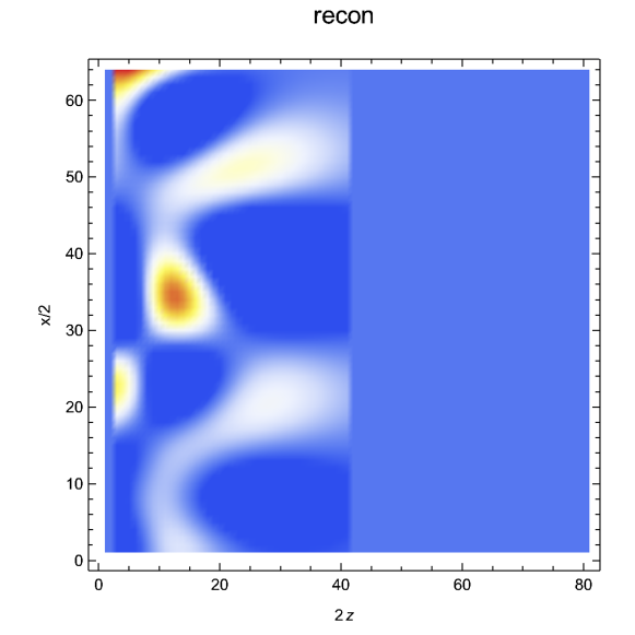
Figure 4. The reconstructed $\mu_{a}$ in (82).

5. Concluding remarks

In this paper, the time-resolved measurement for the stripe illumination was proposed. The penetration depth of near-infrared light can be controlled with the pitch $L$ of the stripe.

Although the diffuse optical tomography was tested by using the forward data from Monte Carlo simulation, the proposed impulse stripe illumination will be realized by single-photon avalanche diode (SPAD) arrays [5].

In the present formulation, the bright part of the stripe illumination was modeled by the Dirac delta function as shown in (24). It is a future issue to consider the finite width of the stripe.

Since the proposed optical tomography uses time-resolved data, a natural next step is the reconstruction of both the absorption and reduced scattering coefficients. The reconstruction of two parameters by the Rytov approximation [6] will be utilized for the stripe illumination.

Funding.

MM acknowledges support from JSPS KAKENHI Grant No. JP17K05572 and JP18K03438, and JST PRESTO Grant Number JPMJPR2027. KK acknowledges support from JSPS KAKENHI Grant No. JP16K04985, JP17H06102, JP18H01497, JP18H05240.

Disclosures.

The authors declare no conflicts of interest.

Appendix A Green’s function

Let us consider the Green’s function which satisfies (5). The Fourier transform is employed as

$$\widetilde{G}(\boldsymbol{\mathrm{q}},z,\boldsymbol{\mathrm{r}}^{\prime})=\int_{\mathbb{R}^{2}}e^{-i\boldsymbol{\mathrm{q}}\cdot\boldsymbol{\mathrm{\rho}}}G(\boldsymbol{\mathrm{r}},\boldsymbol{\mathrm{r}}^{\prime})\,d\boldsymbol{\mathrm{\rho}}.$$ (83)

We have

$$\left\{\begin{aligned} \partial_{z}^{2}\widetilde{G}-\lambda(q)^{2}\widetilde{G}=\frac{-1}{D_{0}}e^{-i\boldsymbol{\mathrm{q}}\cdot\boldsymbol{\mathrm{\rho}}^{\prime}}\delta(z-z^{\prime}),&\quad z>0,\\ -z_{e}\partial_{z}\widetilde{G}+\widetilde{G}=0,&\quad z=0.\end{aligned}\right.$$ (84)

We can write

$$\widetilde{G}=\left\{\begin{aligned} A_{1}e^{\lambda z}+A_{2}e^{-\lambda z},&\quad 0<z<z^{\prime},\\ Be^{-\lambda z},&\quad z>z^{\prime}.\end{aligned}\right.$$ (85)

We have

$$(1-\lambda z_{e})A_{1}+(1+\lambda z_{e})A_{2}=0,$$ (86)

$$A_{1}e^{\lambda z^{\prime}}+A_{2}e^{-\lambda z^{\prime}}=Be^{-\lambda z^{\prime}},$$ (87)

and the jump condition

$$-Be^{-\lambda z^{\prime}}-A_{1}e^{\lambda z^{\prime}}+A_{2}e^{-\lambda z^{\prime}}=\frac{-1}{\lambda D_{0}}e^{-i\boldsymbol{\mathrm{q}}\cdot\boldsymbol{\mathrm{\rho}}^{\prime}}.$$ (88)

From the conditions (86), (87), and (88), we obtain

$$A_{1} =\frac{1}{2\lambda D_{0}}e^{-i\boldsymbol{\mathrm{q}}\cdot\boldsymbol{\mathrm{\rho}}^{\prime}}e^{-\lambda z^{\prime}},$$ (89)

$$A_{2} =\frac{z_{e}\lambda-1}{z_{e}\lambda+1}\frac{1}{2\lambda D_{0}}e^{-i\boldsymbol{\mathrm{q}}\cdot\boldsymbol{\mathrm{\rho}}^{\prime}}e^{-\lambda z^{\prime}},$$

$$B =\frac{1}{2\lambda D_{0}}e^{-i\boldsymbol{\mathrm{q}}\cdot\boldsymbol{\mathrm{\rho}}^{\prime}}\left(e^{\lambda z^{\prime}}+\frac{z_{e}\lambda-1}{z_{e}\lambda+1}e^{-\lambda z^{\prime}}\right).$$

Let $z^{\prime}\to 0$. We obtain

$$\widetilde{G}(\boldsymbol{\mathrm{q}},z,\boldsymbol{\mathrm{r}}^{\prime})=\frac{z_{e}}{D_{0}}e^{-i\boldsymbol{\mathrm{q}}\cdot\boldsymbol{\mathrm{\rho}}^{\prime}}\frac{1}{z_{e}\lambda(q)+1}e^{-\lambda(q)z},\quad z>0,\quad z^{\prime}=0.$$ (90)

Therefore,

$$G(\boldsymbol{\mathrm{r}},\boldsymbol{\mathrm{r}}^{\prime}) =\frac{1}{(2\pi)^{2}}\int_{\mathbb{R}^{2}}e^{i\boldsymbol{\mathrm{q}}\cdot\boldsymbol{\mathrm{\rho}}}\widetilde{G}(\boldsymbol{\mathrm{q}},z,\boldsymbol{\mathrm{r}}^{\prime})\,d\boldsymbol{\mathrm{q}}$$ (91)

$$=\frac{z_{e}}{(2\pi)^{2}D_{0}}\int_{\mathbb{R}^{2}}e^{i\boldsymbol{\mathrm{q}}\cdot(\boldsymbol{\mathrm{\rho}}-\boldsymbol{\mathrm{\rho}}^{\prime})}\frac{e^{-\lambda(q)z}}{1+\lambda(q)z_{e}}\,d\boldsymbol{\mathrm{q}},\quad z>0,\quad z^{\prime}=0.$$

We have

$$G(\boldsymbol{\mathrm{r}}_{0},\boldsymbol{\mathrm{r}}_{s}) =\frac{z_{e}}{(2\pi)^{2}D_{0}}\int_{\mathbb{R}^{2}}e^{-iq_{x}(x_{0}-x_{s})}\frac{e^{-\lambda(q)z_{0}}}{1+\lambda(q)z_{e}}\,d\boldsymbol{\mathrm{q}}$$ (92)

$$=\frac{z_{e}}{(2\pi)^{2}D_{0}}\int_{0}^{2\pi}\int_{0}^{\infty}e^{-iq(x_{0}-x_{s})\cos\varphi}\frac{e^{-\lambda(q)z_{0}}}{1+\lambda(q)z_{e}}q\,dqd\varphi$$

$$=\frac{z_{e}}{2\pi D_{0}}\int_{0}^{\infty}qJ_{0}(q|x_{0}-x_{s}|)\frac{e^{-\lambda(q)z_{0}}}{1+\lambda(q)z_{e}}\,dq.$$

Similarly we have

$$G(\boldsymbol{\mathrm{r}}_{0},\boldsymbol{\mathrm{r}}_{d})=\frac{z_{e}}{2\pi D_{0}}\int_{0}^{\infty}qJ_{0}(q|x_{0}-x_{d}|)\frac{e^{-\lambda(q)z_{0}}}{1+\lambda(q)z_{e}}\,dq.$$ (93)

Appendix B Computation of $H_{\omega}$

The function $H_{\omega}$ in (45) is written as

$$H_{\omega}(x,z,z^{\prime})=\int_{0}^{\infty}F(q;x,z,z^{\prime})\,dq,$$ (94)

where

$$F(q;x,z,z^{\prime}) =\frac{1}{2\pi D_{0}Q_{\omega}(q)}\cos(qx)$$ (95)

$$\times\left[e^{-Q_{\omega}(q)|z-z^{\prime}|}-\frac{1-Q_{\omega}(q)z_{e}}{1+Q_{\omega}(q)z_{e}}e^{-Q_{\omega}(q)|z+z^{\prime}|}\right].$$

The integral can be evaluated by the double-exponential formula [7, 8, 9]. Define

$$\phi(\tau)=\frac{\tau}{1-e^{-6\sinh{\tau}}}$$ (96)

with

$$\phi^{\prime}(\tau)=\frac{1-(1+6\tau\cosh{\tau})e^{-6\sinh{\tau}}}{\left(1-e^{-6\sinh{\\ tau}}\right)^{2}}.$$ (97)

We have

$$\int_{0}^{\infty}F(q;x,z,z^{\prime})\,dq\approx\frac{\pi}{|x|}\sum_{k=-N_{k}}^{N_{k}}F\left(\frac{\pi}{h|x|}\phi\left(kh+\frac{h}{2}\right);x,z,z^{\prime}\right)$$ (98)

$$\times\phi^{\prime}\left(kh+\frac{h}{2}\right),$$

where $N_{k}>0$ is an integer and $h$ is a mesh size.

Appendix C Pseudoinverse

Let us consider

$$\boldsymbol{\mathrm{\eta}}=\underline{J}_{\rm reg}^{+}\boldsymbol{\mathrm{\psi}}.$$ (99)

C.1. Underdetermined

In this case,

$$\underline{J}_{\rm reg}^{+}=\underline{J}^{*}\underline{M}_{\rm reg}^{-1},\quad\underline{M}=\underline{J}\,\underline{J}^{*}.$$ (100)

Here, $*$ denotes the Hermitian conjugate and ${\rm reg}$ means that the pesudoinverse is regularized by discarding singular values that are smaller than $\sigma_{0}$. Let $\sigma_{j}^{2}$ and $\boldsymbol{\mathrm{v}}_{j}$ be the eigenvalues and eigenvectors of the matrix $\underline{M}$:

$$\underline{M}\boldsymbol{\mathrm{z}}_{j}=\sigma_{j}^{2}\boldsymbol{\mathrm{z}}_{j}.$$ (101)

We obtain

$$\boldsymbol{\mathrm{\eta}}=\sum_{j\atop\sigma_{j}>\sigma_{0}}\frac{1}{\sigma_{j}^{2}}\left(\boldsymbol{\mathrm{z}}_{j}^{*}\boldsymbol{\mathrm{\psi}}\right)\underline{J}^{*}\boldsymbol{\mathrm{z}}_{j}.$$ (102)

C.2. Overdetermined

In this case,

$$\underline{J}_{\rm reg}^{+}=\underline{M}_{\rm reg}^{-1}\underline{J}^{*},\quad\underline{M}=\underline{J}^{*}\,\underline{J}.$$ (103)

After solving the eigenproblem $\underline{M}\boldsymbol{\mathrm{z}}_{j}=\sigma_{j}^{2}\boldsymbol{\mathrm{z}}_{j}$, we obtain

$$\boldsymbol{\mathrm{\eta}}_{1}=\sum_{j\atop\sigma_{j}>\sigma_{0}}\frac{1}{\sigma_{j}^{2}}\left(\boldsymbol{\mathrm{z}}_{j}^{*}\underline{J}^{*}\boldsymbol{\mathrm{\psi}}\right)\boldsymbol{\mathrm{z}}_{j}.$$ (104)

References

[1]
D. J. Cuccia, F. Bevilacqua, A. J. Durkin, F. R. Ayers, and B. J. Tromberg,
“Quantitation and mapping of tissue optical properties using modulated imaging,”
J. Biomed. Opt. 14, 024012 (2009).
[2]
C. Hock, K. Villringer, F. Müller-Spahn, R. Wenzel, H. Heekeren, S. Schuh-Hofer, M. Hofmann, S. Minoshima, M. Schwaiger, U. Dirnagl, and A. Villringer,
“Decrease in parietal cerebral hemoglobin oxygenation during performance of a verbal fluency task in patients with Alzheimer’s disease monitored by means of near-infrared spectroscopy (NIRS)–correlation with simultaneous rCBF-PET measurements,”
Brain Res. 755, 293–303 (1997).
[3]
V. Quaresima and M. Ferrari,
“Functional near-infrared spectroscopy (fNIRS) for assessing cerebral cortex function during human behavior in natural/social situations: A concise review,”
Org. Res. Meth. 22, 46–68 (2019)
[4]
M. Machida, Y. Hoshi, K. Kagawa, and K. Takada,
“Decay behavior and optical parameter identification for spatial-frequency domain imaging by the radiative transport equation,”
J. Opt. Soc. Am. A 37, 2020–2031 (2020).
[5]
C. Bruschini, H. Homulle, I. M. Antolovic, S. Burri, and E. Charbon,
“Single-photon avalanche diode imagers in biophotonics: review and outlook”
Light: Sci. Appl. 8, 87 (2019).
[6]
V. A. Markel and J.n C. Schotlan,
“Symmetries, inversion formulas, and image reconstruction for optical tomography,”
Phys. Rev. E 70, 056616 (2004).
[7]
T. Ooura and M. Mori,
“The double exponential formula for oscillatory functions over the half infinite interval,”
J. Comput. Appl. Math. 38, 353–360 (1991).
[8]
T. Ooura and M. Mori,
“A robust double exponential formula for Fourier-type integrals,”
J. Comput. Appl. Math. 112, 229–241 (1999).
[9]
H. Ogata,
“A numerical integration formula based on the Bessel functions,”
Publ. RIMS, Kyoto Univ. 41, 949–970 (2005).