Imprints of LGI violation in Mesons

Kiran Sharma kirans@iitbhilai.ac.in Department of Physics, Indian Institute of Technology Bhilai, India    Aryabrat Mahapatra 21ph05015@iitbbs.ac.in School of Basic Sciences, Indian Institute of Technology Bhubaneswar, India    Prasanta K. Panigrahi panigrahi.iiser@gmail.com Indian Institute of Science Education and Research Kolkata, India    Sudhanwa Patra sudhanwa@iitbhilai.ac.in Department of Physics, Indian Institute of Technology Bhilai, India
Abstract

Quantum mechanics has always proven emphatically as one of the main cornerstones in all of the science since its inception. Initially, it has also faced many skeptics from many scientific proponents of its complete description of reality. However, John Bell once devised a theorem on quantitative grounds to show how local realism is expressed in quantum mechanics. As Bell’s inequality claims the non-existence of local hidden variable theories, on the same footing we have Leggett-Garg’s Inequality (LGI), which sets a quantum-classical limit for temporally correlated quantum systems. In the context of particle physics specially in the field of neutrino and meson oscillations, one can conveniently implement LGI to test the quantum foundations at the probability level. Here, we discuss the significant LGI violation characteristics in B- and K-mesons oscillations taking into account their decoherence, CP violation and decay parameters. Also, we discuss and comment on the behavior or effect of decoherence and decay widths playing out from the perspective of LGI by taking their available values from various experiments. This may help us to understand the underlying principles and techniques of neutral meson open quantum systems.

Introduction:-
Right from the advent of quantum mechanics, we saw appealing success in all of its predictions and found flourishing consistent results based on real-life applications. However, some scientific proponents questioned the very core ideas and principles of quantum mechanics. Among them, the most notable strike came in 1935, when Albert Einstein, Boris Podolsky and Nathan Rosen published the famous EPR paradox EPR claimed doubts about the indeterministic framework and formalism of quantum mechanics. The fundamental assumption on which EPR argument rest is the principle of locality  Griffith . They argued the interpretation of Copenhagen formalism is incomplete where wave functions instantaneously collapse upon apparently non-local measurement. They propose the non-local hidden variable theory in order to make quantum mechanics deterministic or to preserve the common sense locality. However, in 1964, John Bell devised a quantitative mechanism through inequalities to test these hidden variable theories. It was found that these theories violate Bell’s inequality and are incompatible with quantum mechanics. These Bell inequalities turn the EPR argument completely on its head and forbids any local hidden variable theory and indeed, it proves that any correlations that arise in quantum mechanics cannot arise in any classical or macroscopic system.

In the same outline, Leggett and Garg introduced Leggett-Garg Inequality LGI which attempts to test quantum foundations in various correlated quantum systems by considering certain classical assumptions. This mathematical inequality fulfills the macroscopic physical theories and explains the quantum behavior upon its violation just like Bell inequality. We will implement this technique in open quantum systems open_quantum_system of the neutral meson-antimeson oscillatory system which is a two-state decaying system that can act as a bipartite entangled system.

In this work, we have started with setting up the measurement inequalities from the LGI formalism. Then, we have given a formal introduction to the fundamental description of meson oscillations and their respective probabilities, where we have assumed that CP remains conserved in the entire propagation states of mesons. Further, we have extended our oscillatory systems by laying down a more general description where we not only take account of their CP violation but also treat them as open quantum systems. We calculated their probabilities and drew their correlation with LGI function. Finally, we thoroughly analyzed the behavior of LGI function in response to various intervals of time. Although, there has been a lot of successful work done on this subject correlation ; Banerjee:2014vga ; Naikoo:2019gme ; Naikoo:2018vug ; Budroni ; Naikoo:2019eec ; Naikoo:2017fos ; Dixit ; Gangopadhyay ; Saha ; Shafaq:2021lju ; Joarder ; however, we have highlighted certain imprints of LGI violations that attempt to bring out some specific behavior of LGI function, which is perhaps unique and distinct from other works. We have collectively shown various definite combinations of decay and decoherence effects in our open meson quantum systems. From there, we have specifically studied the amount of violation of LGI function and how close the violation goes to the maximal violation of the quantum mechanical system, then we infer it with intuitive arguments and interpretations. Also in the end, we spotted a very peculiar behavior of LGI function when we formulate our system consistent with CP conservation.

I Theoretical framework

In this section, we will resort to the understanding of the theoretical background of LGI and meson oscillations. We generalize a methodology to define a correlation function in LGI in terms of macroscopic variables which can only take two values. This mechanism has wide applicability in testing LGI violation from photon systems photons to diamond defect centers, NMR systems NMR , solar neutrinos neutrinos ; Shafaq:2021lju and more. Then we will discuss the phenomenology of the two-state oscillatory system of K- and B-mesons which are generally produced in strong and electromagnetic interactions and they decay by weak interactions. Finally, we will be using the probabilistic approach of decaying systems decay ; correlation to study various measures of quantum correlations in $B\bar{B}$ and $K\bar{K}$ oscillation systems.

I.1 LGI Formalism:

The sole motive to propose LGI is to understand how macroscopic realism accounts for quantum systems and how the idea of certainties and superposition of the classical world can govern the principles in the microscopic domain. The assumptions on which the entire paradigm of LGI rests are macroscopic realism and noninvasive measurability Assumptions . According to Leggett and Garg, macroscopic realism is the worldview in which attributes of macroscopic systems exist independent of external measurement and observation. And noninvasive measurability says that a result of observation is not influenced anyway by the mere act of measurement unlike what Copenhagen interpretation demands. Classical physics works definitively very well relying on these assumptions, while quantum mechanics goes downright inconsistent.

I.1.1 Setting up LGI in terms of correlation functions:

Suppose, if we consider a macroscopic variable that can take on two values, $Q=\pm 1$, and its two-time correlation function neutrinos

$\displaystyle C_{ij}=\langle\hat{Q(t_{i})}\hat{Q(t_{j})}\rangle$ (1)

where $\hat{Q(t)}$ is the operator corresponding to the observable Q.If macroscopic realism and noninvasive measurability are obeyed, then the Leggett-Garg inequality places classical limits on a combination of the correlations: for three measurements,

$\displaystyle-3\leq C_{12}+C_{23}-C_{13}\leq 1$ (2)

In general, there can be LGIs corresponding to an n-measurement Leggett-Garg parameter,

$\displaystyle-n\leq K_{n}\leq n-2,\hskip 8.2511ptn=3,5,7,..$
$\displaystyle-(n-2)\leq K_{n}\leq n-2,\hskip 8.2511ptn=4,5,6,..$ (3)

where, $K_{n}=C_{12}+...+C_{n-1\hskip 1.42271ptn}-C_{n1}$ We can prove these inequalities in the following way:
The correlation function $C_{ij}$ is defined as;

$\displaystyle C_{ij}=\sum_{Q_{i},Q_{j}=\pm 1}Q_{i}Q_{j}P_{ij}(Q_{i},Q_{j})$ (4)

where $P_{i,j}(Q_{i},Q_{j})$ is the joint probability of measuring $Q_{i}=\pm 1$ at time $t_{i}$ and $Q_{j}=\pm 1$ at time $t_{j}$
Now, we can express the above joint probability in terms of some third possible measurement observable at a different time taking these same values;

$\displaystyle P_{ij}(Q_{i},Q_{j})=\sum_{Q_{k}=\pm 1,k\neq i,j}P_{ij}(Q_{1},Q_{2},Q_{3})$ (5)

where $Q_{3}$ is the value of Q at $t=t_{3}$.

So, we know $K_{3}=C_{12}+C_{23}-C_{13}$ and hence $K_{3}$ can be written as

$\displaystyle K_{3}=\sum_{Q_{i},Q_{j}=\pm 1}(\sum_{Q_{k},k\neq 1,2}P(Q_{1},Q_{2},Q_{3})+$
$\displaystyle\sum_{Q_{k},k\neq 2,3}P(Q_{1},Q_{2},Q_{3})-\sum_{Q_{k},k\neq 1,3}P(Q_{1},Q_{2},Q_{3}))$ (6)

Now, using the fact of normalization of probabilities, we can write, $\Sigma=1$. So, then $K_{3}$ will reduce to the equation;

$\displaystyle K_{3}=1-4\left(P(+,-,+)+P(-,+,-)\right)$ (7)

Then the minimum and maximum bounds for $K_{3}$ will go as:

$\displaystyle-3\leq C_{12}+C_{23}-C_{13}\leq 1$ (8)

Finally, equation (8) gives the so-called Leggett-Garg Inequality for a three-measurement correlation.

I.1.2 LGI Violation

As this correlation function has been laid out based on classical assumption, so they can be well treated as classical physical observables. If this is so, then classical observables commute with each other and so they follow the symmetric relation among them. Thus, the correlation function $C_{ij}=\langle Q_{i}Q_{j}\rangle$ can be given as:

$\displaystyle C_{ij}=\frac{1}{2}\langle Q_{i}Q_{j}+Q_{j}Q_{i}\rangle$ (9)

Suppose, let we view these parameters as quantum mechanical observables. It can be possible to express them in the basis of the linear combination of Pauli matrices i.e., $\hat{Q_{i}}={\boldsymbol{a_{i}}}.\hat{\sigma}$, then we find that

$\displaystyle C_{ij}$ $\displaystyle=$ $\displaystyle\frac{1}{2}\langle Q_{i}Q_{j}+Q_{j}Q_{i}\rangle={\boldsymbol{a_{i}}}.{\boldsymbol{a_{j}}}$ (10)
$\displaystyle\left(\because({\boldsymbol{\sigma}}.{\boldsymbol{A}})({\boldsymbol{\sigma}}.{\boldsymbol{B}})={\boldsymbol{A}}.{\boldsymbol{B}}+i{\boldsymbol{\sigma}}.({\boldsymbol{A}}\times{\boldsymbol{B}})\right)$
$\displaystyle\implies K_{3}$ $\displaystyle=$ $\displaystyle\cos{\theta_{1}}+\cos{\theta_{2}}-\cos{(\theta_{1}+\theta_{2})}$ (11)

where, $\theta_{1}$ is the angle between vectors ${\boldsymbol{a_{1}}}$ and ${\boldsymbol{a_{2}}}$, $\theta_{2}$ is between vectors ${\boldsymbol{a_{2}}}$ and ${\boldsymbol{a_{3}}}$.

Now, to get the upper limit of $K_{3}$, we have to choose a specific set of value for $\theta s$. We see when $\theta_{1}=\theta_{2}=\theta_{3}=\frac{\pi}{3}$ we get the maximum value of $K_{3}$:

$\displaystyle max(K_{3})=1.5$ (12)

This is beyond the predicted value of LGI, hence these quantum mechanical observables indeed violates the inequality.

Now, we can draw an analogy between LGI and Bell Inequality. Since, we saw again in quantum mechanics unlike classical observables we find,

$\displaystyle\left[Q_{i},Q_{j}\right]=2i\hat{\sigma}.({\boldsymbol{a_{i}}}\times{\boldsymbol{a_{j}}})$ (13)

instead of zero. Thus, it violates LGI in the quantum regime. Bell inequality sets a lower bound and an upper bound for spatially correlated events. Similarly, LGI sets the limits for temporally correlated events. Hence, LGIs are also known as temporal Bell inequalities.

I.2 K- and B-Mesons Oscillations:

Mesons are the class of subatomic particles composed of a quark and an anti-quark bound state. These quark and anti-quark bound states are found as $\pi^{+}(u\bar{d})$, $\pi^{-}(u\bar{d})$, $K^{0}(\bar{s}d)$, $K^{+}(\bar{s}u)$, $\bar{K^{0}}(s\bar{d})$, $B^{0}_{d}(d\bar{b})$, $\bar{B^{0}_{s}}(\bar{s}b)$, etc. with charges 1, -1, 0, 1, 0, 0, 0. The neutral K meson, $K^{0}$ and B meson, $B^{0}$ and their respective antiparticles, $\bar{K^{0}}$ and $\bar{B^{0}}$ form a very exceptional quantum-mechanical two-state system, which has many key roles in elementary particle physics. Their physics has helped us to unveil frameworks to understand various aspects such as prediction of quark masses, study of CKM matrix and their mixing ratios, and the amount of CP asymmetries in their respective decays. These mesons are generally produced in strong or electromagnetic interactions, which conserves their quark flavor, and they decay by weak interactions. Since the mesons are unstable, they eventually decay into lighter mesons having lighter quark masses and also into neutrinos, electrons, etc.; or in other words, they can decay semi-leptonically ($l$, $\nu_{l}$ and $\pi$) or hadronically ($\pi$). In semileptonic decays of K-mesons into the final state of pions with a particular distinct charge;

$$K^{0}\rightarrow l^{+}\nu_{l}\pi^{-}\hskip 12.80365pt\bar{K^{0}}\rightarrow l^{-}\bar{\nu_{l}}\pi^{+}$$

For hadronic decays, these K-mesons can result in two or three pions depending upon the state of superposition of $K^{0}$ and $\bar{K^{0}}$. Suppose, if we take the system of $K^{0}\bar{K^{0}}$ vacuum oscillation with the assumption of CP conservation in the decay of neutral kaons in the weak interaction. In this regard, the observed states of kaons will appear:

$\displaystyle|K_{1}^{0}\rangle=\frac{1}{\sqrt{2}}\left[|K^{0}\rangle+|\bar{K^{0}}\rangle\right]$ (14)
$\displaystyle|K_{2}^{0}\rangle=\frac{1}{\sqrt{2}}\left[|K^{0}\rangle-|\bar{K^{0}}\rangle\right]$ (15)

$|K_{1}^{0}\rangle$ and $|K_{2}^{0}\rangle$ are the physical states that are available and are referred as short-lived mass eigenstates with proper lifetime $\tau_{1}$ and long-lived mass eigenstates with proper lifetime $\tau_{2}$ respectively. Each of them has a unique life-time. According to the assumptions these linear combination states will form the CP eigenstates.

$\displaystyle\hat{C}\hat{P}|K_{1}^{0}\rangle=+|K_{1}^{0}\rangle$ (16)
$\displaystyle\hat{C}\hat{P}|K_{2}^{0}\rangle=-|K_{2}^{0}\rangle$ (17)

Also, these states can be expressed back for $|K^{0}\rangle$ and $|\bar{K^{0}}\rangle$ states;

$\displaystyle|K^{0}\rangle=\frac{1}{\sqrt{2}}\left[|K_{1}^{0}\rangle+|K_{2}^{0}\rangle\right]$ (18)
$\displaystyle|\bar{K^{0}}\rangle=\frac{1}{\sqrt{2}}\left[|K_{1}^{0}\rangle-|K_{2}^{0}\rangle\right]$ (19)

Further if we wish to study the decay effects of kaons in a particular direction (say z) then by virtue of conservation of angular momentum the whole composite system of kaons will be correlated by the standard singlet configuration;

$\displaystyle|\Phi\rangle$ $\displaystyle=$ $\displaystyle\frac{1}{\sqrt{2}}\left[|K^{0}(z)\bar{K^{0}}(-z)\rangle+|\bar{K^{0}}(z)|K^{0}(-z)\rangle\right]$ (20)
$\displaystyle=$ $\displaystyle\frac{1}{\sqrt{2}}\left[|K_{2}^{0}(z)K_{1}^{0}(-z)\rangle+|K_{1}^{0}(z)K_{2}^{0}(-z)\rangle\right]$

The evolution of a $K^{0}\bar{K^{0}}$ oscillatory system in time can be studied by the time dependent Schrödinger equation:

$\displaystyle i\frac{d}{dt}\begin{pmatrix}K^{0}(t)\\ \bar{K^{0}}(t)\end{pmatrix}=\begin{pmatrix}H_{11}&H_{12}\\ H_{21}&H_{22}\end{pmatrix}\begin{pmatrix}K^{0}(t)\\ \bar{K^{0}}(t)\end{pmatrix}$ (21)

The Hamiltonian matrix is composed of a hermitian $M$, the energy part of the oscillation and also an anti-hermitian $\Gamma$ which is responsible for the decay of oscillations and is equal to the inverse of proper lifetime;

$\displaystyle H=M-\frac{i}{2}\Gamma$ (22)

Therefore, the kaon state can be written as:

$\displaystyle\ket{\psi}=\begin{pmatrix}a\\ b\end{pmatrix}=a\begin{pmatrix}1\\ 0\end{pmatrix}+b\begin{pmatrix}0\\ 1\end{pmatrix}$ (23)

where, $\ket{K^{0}}=\begin{pmatrix}1\\ 0\end{pmatrix}$ and $\ket{\bar{K^{0}}}=\begin{pmatrix}0\\ 1\end{pmatrix}$.

Thus,

$\displaystyle\psi(t)=e^{-iHt}\psi(0)$
$\displaystyle\text{or}\hskip 8.5359pt\begin{pmatrix}K^{0}(t)\\ \bar{K^{0}}(t)\end{pmatrix}=e^{-\frac{\Gamma}{2}}e^{-iMt}\begin{pmatrix}K^{0}(0)\\ \bar{K^{0}}(0)\end{pmatrix}$ (24)

If the system initially starts with only $\ket{K^{0}}$ state, then after time $t$, the propagation state will be:

$\displaystyle\ket{\psi(t)}=\frac{1}{\sqrt{2}}\left[e^{-(im_{1}+\Gamma_{1}/2)}\ket{K^{0}_{1}}+e^{-(im_{2}+\Gamma_{2}/2)}\ket{K^{0}_{2}}\right]$

Now, we can determine the corresponding probabilities;

$\displaystyle P_{K^{0}}=\frac{1}{4}\left[e^{-\Gamma_{1}t}+e^{-\Gamma_{2}t}+2e^{-(\Gamma_{1}+\Gamma_{2})t/2}\cos{(\Delta m_{K}t)}\right]$

and

$\displaystyle P_{\bar{K^{0}}}=\frac{1}{4}\left[e^{-\Gamma_{1}t}+e^{-\Gamma_{2}t}-2e^{-(\Gamma_{1}+\Gamma_{2})t/2}\cos{(\Delta m_{K}t)}\right]$

where, $\Delta m_{K}=|m_{1}-m_{2}|$ is $K_{1}^{0}-K_{2}^{0}$ mass difference. Equations (I.2) and (I.2); give the probabilities of state $\ket{K^{0}}$ remaining in the same itself and making the transition to its antiparticle state respectively Radoje . In the same way, we can study the $B^{0}_{d}-\bar{B^{0}_{d}}$ and $B^{0}_{s}-\bar{B^{0}_{s}}$ oscillations (neutral $B$-mesons). We can do the similar time evolution and determine their probabilities with the corresponding neutral B-mesons parameters.

I.3 Quantum Correlations in K- and B-Mesons oscillations:

We have dealt with our systems so far considering a closed quantum system, however the systems which we encounter in real physical systems involve a significant degree of interactions with its environment. So we implement the mathematical formalism of quantum operations which is a very important tool for describing the dynamics of open quantum systems. We have to treat the states involved in our system as some mixed states instead of pure states and evolve them accordingly Banks:1983by . The evolution of states should be carried through considering our system as a sub-system embedded in an exterior environment, thus the evolution of sub-system will differ from the system significantly Nielsen . This will further lead to damping effects in our meson oscillation systems which originates in the form of decoherence in our open quantum states. This quantum decoherence effect can be understood using the Liouville-Lindblad formalism for open quantum systems Lindblad . The evolution of density matrix $\rho$ for the oscillatory system will be governed by;

$\displaystyle\frac{\partial\rho}{\partial t}=-i\left[H,\rho\right]+D[\rho]$ (28)

where $D[\rho]$ is the term that causes the non-unitary evolution of the system, which is termed as decoherence. Here, our sub-system is $K^{0}-\bar{K^{0}}$ meson system which is the principal system, and the environment that it is interacting which is attributed by our action of measurement. The principal system and environment together forms a closed quantum system then our system-environment composite state will be characterized as $\rho\otimes\rho_{env}$. Now, performing a partial trace over the environment we will end up with the reduce state of sub-system alone:

$\displaystyle\mathcal{E}(\rho)=tr_{env}\left[U(\rho\otimes\rho_{env})U^{\dagger}\right]$ (29)

Here, $U$ is responsible for the transformation of entire composite system. If there is any other $\tilde{U}$ operator which only transforms the sub-system alone and has no interaction with environment, then our final state will be as usual $\mathcal{E}(\rho)=\tilde{U}\rho\tilde{U}^{\dagger}$. This can be further put in a elegant representation known as operator-sum representation:

$\displaystyle\mathcal{E}(\rho)$ $\displaystyle=$ $\displaystyle\sum_{i}\bra{e_{i}}U\left[\rho\otimes\ket{e_{0}}\bra{e_{0}}\right]U^{\dagger}\ket{e_{i}}$ (30)
$\displaystyle=$ $\displaystyle\sum_{i}\mathcal{K}_{i}\rho\mathcal{K}_{i}^{\dagger}$

where $\mathcal{K}_{i}=\bra{e_{i}}U\ket{e_{0}}$ is an operator on the state space of the principal system. The operators {$\mathcal{K}_{i}$} are known as operation elements for the quantum operation $\mathcal{E}$. The {$\ket{e_{i}}$} is an orthonormal basis for the environment state space and $\rho_{env}=\ket{e_{0}}\bra{e_{0}}$ is its initial state. The operation elements satisfy the completeness property i.e., $tr(\mathcal{E}(\rho))=1$, this follows $\mathcal{K}_{i}$ operators to feature as trace preserve operations;

$\displaystyle\sum_{i}\mathcal{K}_{i}^{\dagger}\mathcal{K}_{i}=I$ (31)

These $\mathcal{K}_{i}$ are also known as Kraus operators Kraus . Now, as our principal system is $K^{0}-\bar{K^{0}}$ oscillation system, we can choose our orthonormal basis as {$\ket{K^{0}},\ket{\bar{K^{0}}},\ket{0}$}, where $\ket{0}$ is a vacuum state. This basis will span the entire Hilbert space of our composite system Banerjee:2014vga ; Caban ; Naikoo:2019gme .

$\displaystyle\ket{K^{0}}=\begin{pmatrix}1\\ 0\\ 0\end{pmatrix};\ket{\bar{K^{0}}}=\begin{pmatrix}0\\ 1\\ 0\end{pmatrix};\ket{0}=\begin{pmatrix}0\\ 0\\ 1\end{pmatrix}$ (32)

If we proceed ahead with the general case of kaon oscillation by incorporating the CP violation measure Sarkar in the oscillating states, then our new long and short lived states will take the form:

$\displaystyle\ket{K_{S}}=\frac{1}{\sqrt{1+|\epsilon|^{2}}}\left(\ket{K_{1}^{0}}+\epsilon\ket{\bar{K_{2}^{0}}}\right)$
$\displaystyle\ket{K_{L}}=\frac{1}{\sqrt{1+|\epsilon|^{2}}}\left(\epsilon\ket{K_{1}^{0}}+\ket{\bar{K_{2}^{0}}}\right)$ (33)

where $\epsilon$ is the CP violating parameter. Then the evolution of density matrix for our principal system is:

$\displaystyle\rho(t)=\sum_{i=0}\mathcal{K}_{i}(t)\rho(0)\mathcal{K}_{i}^{\dagger}(t)$ (34)

Kraus operators here are expressed in the following way Naikoo:2018vug :

$\displaystyle\mathcal{K}_{0}$ $\displaystyle=$ $\displaystyle\ket{0}\bra{0}$
$\displaystyle\mathcal{K}_{1}$ $\displaystyle=$ $\displaystyle\mathcal{C}_{1+}(\ket{K^{0}}\bra{K^{0}}+\ket{\bar{K^{0}}}\bra{\bar{K^{0}}})$
$\displaystyle+\mathcal{C}_{1-}(\frac{1+\epsilon}{1-\epsilon}\ket{K^{0}}\bra{\bar{K^{0}}}+\frac{1-\epsilon}{1+\epsilon}\ket{\bar{K^{0}}}\bra{K^{0}})$
$\displaystyle\mathcal{K}_{2}$ $\displaystyle=$ $\displaystyle\mathcal{C}_{2}(\frac{1}{1+\epsilon}\ket{0}\bra{K^{0}}+\frac{1}{1-\epsilon}\ket{0}\bra{\bar{K^{0}}})$
$\displaystyle\mathcal{K}_{3}$ $\displaystyle=$ $\displaystyle\mathcal{C}_{3+}\frac{1}{1+\epsilon}\ket{0}\bra{K^{0}}+\mathcal{C}_{3-}\frac{1}{1-\epsilon}\ket{0}\bra{\bar{K^{0}}}$
$\displaystyle\mathcal{K}_{4}$ $\displaystyle=$ $\displaystyle\mathcal{C}_{4}(\ket{K^{0}}\bra{K^{0}}+\ket{\bar{K^{0}}}\bra{\bar{K^{0}}}$
$\displaystyle+\frac{1+\epsilon}{1-\epsilon}\ket{K^{0}}\bra{\bar{K^{0}}}+\frac{1-\epsilon}{1+\epsilon}\ket{\bar{K^{0}}}\bra{K^{0}})$
$\displaystyle\mathcal{K}_{5}$ $\displaystyle=$ $\displaystyle\mathcal{C}_{5}(\ket{K^{0}}\bra{K^{0}}+\ket{\bar{K^{0}}}\bra{\bar{K^{0}}}$ (35)
$\displaystyle-\frac{1+\epsilon}{1-\epsilon}\ket{K^{0}}\bra{\bar{K^{0}}}-\frac{1-\epsilon}{1+\epsilon}\ket{\bar{K^{0}}}\bra{K^{0}})$

The coefficients are as follows:

$\displaystyle\mathcal{C}_{1\pm}$ $\displaystyle=$ $\displaystyle\frac{1}{2}\left[e^{-(2im_{S}+\Gamma_{S}+\lambda)t/2}\pm e^{-(2im_{L}+\Gamma_{L}+\lambda)t/2}\right]$
$\displaystyle\mathcal{C}_{2}$ $\displaystyle=$ $\displaystyle\sqrt{\frac{1+|\epsilon|^{2}}{2}\left(1-e^{-\Gamma_{S}t}-\delta_{L}^{2}\frac{|1-e^{-(\Gamma+\lambda-i\Delta m)t}|^{2}}{1-e^{-\Gamma_{L}t}}\right)}$
$\displaystyle\mathcal{C}_{3\pm}$ $\displaystyle=$ $\displaystyle\sqrt{\frac{1+|\epsilon|^{2}}{2(1-e^{-\Gamma_{L}t})}}\left[1-e^{-\Gamma_{L}t}\pm(1-e^{-(\Gamma+\lambda-i\Delta m)t})\right]$
$\displaystyle\mathcal{C}_{4}$ $\displaystyle=$ $\displaystyle\frac{e^{-\Gamma_{S}t/2}}{2}\sqrt{1-e^{-\lambda t}}$
$\displaystyle\mathcal{C}_{5}$ $\displaystyle=$ $\displaystyle\frac{e^{-\Gamma_{L}t/2}}{2}\sqrt{1-e^{-\lambda t}}$ (36)

Now, for the evolution of density matrices for the oscillations of $K^{0}-\bar{K^{0}}$, we can evolve it by the help of these Kraus operators.
When the system was initially at $\ket{K^{0}}$ state:

$\displaystyle\rho_{K^{0}}(t)$ $\displaystyle=$ $\displaystyle\sum_{i}\mathcal{K}_{i}\rho_{K^{0}}(0)\mathcal{K}_{i}^{\dagger}$
$\displaystyle=$ $\displaystyle\mathcal{K}_{0}\rho_{K^{0}}(0)\mathcal{K}_{0}^{\dagger}+\mathcal{K}_{1}\rho_{K^{0}}(0)\mathcal{K}_{1}^{\dagger}+...+\mathcal{K}_{5}\rho_{K^{0}}(0)\mathcal{K}_{5}^{\dagger}$

Similarly, if the system was initially at $\ket{\bar{K^{0}}}$ state:

$\displaystyle\rho_{\bar{K^{0}}}(t)$ $\displaystyle=$ $\displaystyle\sum_{i}\mathcal{K}_{i}\rho_{\bar{K^{0}}}(0)\mathcal{K}_{i}^{\dagger}$ (38)

The $\rho_{K^{0}}(0)$ and $\rho_{\bar{K^{0}}}(0)$ are the corresponding initial density operators for the pure states $\ket{K^{0}}\bra{K^{0}}$ and $\ket{\bar{K^{0}}}\bra{\bar{K^{0}}}$ respectively. Using these, we can construct the respective evolved density operators (as solved in Appendix [A]) from equations (I.3) and (I.3) in the following form:

$\displaystyle\rho_{K^{0}}(t)=\frac{1}{2}e^{-\Gamma t}\begin{pmatrix}a_{ch}+e^{-\lambda t}a_{c}&(\frac{1-\epsilon}{1+\epsilon})^{*}(-a_{sh}-ie^{-\lambda t}a_{s})&0\\ (\frac{1-\epsilon}{1+\epsilon})(-a_{sh}+ie^{-\lambda t}a_{s})&|\frac{1-\epsilon}{1+\epsilon}|^{2}(a_{ch}-e^{-\lambda t}a_{c})&0\\ 0&0&\rho_{33}(t)\\ \end{pmatrix}$
$\displaystyle\rho_{\bar{K^{0}}}(t)=\frac{1}{2}e^{-\Gamma t}\begin{pmatrix}|\frac{1+\epsilon}{1-\epsilon}|^{2}(a_{ch}+e^{-\lambda t}a_{c})&(\frac{1+\epsilon}{1-\epsilon})(-a_{sh}+ie^{-\lambda t}a_{s})&0\\ (\frac{1+\epsilon}{1-\epsilon})^{*}(-a_{sh}-ie^{-\lambda t}a_{s})&(a_{ch}-e^{-\lambda t}a_{c})&0\\ 0&0&\tilde{\rho_{33}}(t)\\ \end{pmatrix}$ (39)

The notations used for the matrix elements denotes these following terms:

  • $a_{ch}=\cosh{\left(\frac{\Delta\Gamma t}{2}\right)}$

  • $a_{sh}=\sinh{\left(\frac{\Delta\Gamma t}{2}\right)}$

  • $a_{c}=\cos{(\Delta mt)}$

  • $a_{s}=\sin{(\Delta mt)}$

  • $\epsilon=\text{CP violating parameter}$

  • $\Delta\Gamma=\Gamma_{S}-\Gamma_{L}$, difference of decay widths

  • $\Gamma=\frac{1}{2}(\Gamma_{L}+\Gamma_{S})$ is the mean decay width

  • $\Delta m=m_{L}-m_{S}$, mass difference

Equations (I.3), give density matrices at time $t$, whose diagonal elements give probabilities for making transition from one state to the other at time $t$, and all other off-diagonal elements describe the superposition states of all states involved. If the initial system starts out with state $\ket{\bar{K^{0}}}$ and probability of remaining in the same state at time $t$ will therefore be given by;

$\displaystyle P_{\bar{K}^{0}\bar{K}^{0}}=\frac{e^{-\Gamma t}}{2}\left[\cosh{\left(\frac{\Delta\Gamma t}{2}\right)}+e^{-\lambda t}\cos{(\Delta mt)}\right]$ (40)

Similarly, other probabilities at time $t$ can be found from the density matrices in equations (I.3).

II Analysis for $3$-measurement LGI parameter $K_{3}$

The two-time correlations which is defined in equation (4), can now be redefined in the context of Kraus operators Castillo ; Paz ; Huelga ; Kofler .

$\displaystyle C(t_{i},t_{j})$ $\displaystyle=$ $\displaystyle p(^{+}t_{i})q(^{+}t_{j}|^{+}t_{i})-p(^{+}t_{i})q(^{-}t_{j}|^{+}t_{i})$
$\displaystyle-p(^{-}t_{i})q(^{+}t_{j}|^{-}t_{i})+p(^{-}t_{i})q(^{-}t_{j}|^{-}t_{i})$

Here, $p(^{a}t_{i})$ gives the probability of getting the result $a=\pm 1$ at $t_{i}$ means initially the system has this probability of remaining in one of the states corresponding to the value of $a=\pm 1$ and $q(^{b}t_{j}|^{a}t_{i})$ gives the conditional probability (or also known as transition probability) which describes that the system has this probability of making transition to another state or remaining in that state (i.e., $b=\pm 1$) at $t_{j}$ given that the system in the either of one state corresponding to $a=\pm 1$ at $t_{i}$. We know that the probability of a quantum state ($\ket{\psi}=\sum_{i}c_{i}\ket{\phi_{i}}$) to be in one of its basis state is equal to the expectation value of projector operator corresponding to that basis state, i.e., $|c_{i}|^{2}=\langle\hat{P_{i}}\rangle$, where $\hat{P_{i}}$ is the projector operator for that basis state. This expectation value further with its density operator can be expressed as $\langle\hat{P_{i}}\rangle=Tr\{\hat{P_{i}}\hat{\rho}\}$. Thus, we can define the probabilities in equation (II) as:

$\displaystyle p(^{a}t_{i})=Tr\{\Pi^{a}\rho(t_{i})\}=Tr\{\Pi^{a}\sum_{\mu}\mathcal{K}_{\mu}(t_{i})\rho(0)\mathcal{K}_{\mu}^{\dagger}(t_{i})\}$

where, $\Pi^{a}$ is the density operator for the dichotomic operator $\hat{Q}$ depending on the value of $a=\pm 1$. Here, we can take $a=+1$ for $\ket{K^{0}}$ and $a=-1$ for $\ket{\bar{K^{0}}}$, $\ket{0}$ states for $Q$ observable and LGI parameter $K_{3}$ in equation(8) will still remain the same Budroni . Further, dichotomic operator can be defined as $\Pi=\Pi^{+}-\Pi^{-}=\Pi_{K^{0}}-(\Pi_{\bar{K^{0}}}+\Pi_{0})$, where $\Pi_{x}=\ket{x}\bra{x}$ Wilde . Also, since $|c_{i}|^{2}=\langle\hat{P_{i}}\rangle$, i.e., $\bra{\psi_{i}}\rho\ket{\psi_{i}}=Tr\{\hat{P_{i}}\hat{\rho}\}$ or in our case $\bra{\psi_{a}}\rho\ket{\psi_{a}}=Tr\{\Pi^{a}\rho\}$, then we can show;

$\displaystyle\rho^{a}$ $\displaystyle=$ $\displaystyle\ket{\psi_{a}}\bra{\psi_{a}}=\ket{\psi_{a}}\left(\frac{\bra{\psi_{a}}\rho\ket{\psi_{a}}}{Tr\{\Pi^{a}\rho\}}\right)\bra{\psi_{a}}$
$\displaystyle\implies\rho^{a}(t_{i})$ $\displaystyle=$ $\displaystyle\frac{\Pi^{a}\rho(t_{i})\Pi^{a}}{Tr\{\Pi^{a}\rho(t_{i})\}}$ (43)
$\displaystyle=$ $\displaystyle\frac{\Pi^{a}\sum_{\mu}\mathcal{K}_{\mu}(t_{i})\rho(0)\mathcal{K}_{\mu}^{\dagger}(t_{i})\Pi^{a}}{p(^{a}t_{i})}$

In order to compute the probability $q(^{b}t_{j}|^{a}t_{i})$, we have to further evolve this density matrix to $t_{j}$, which would go like $\sum_{\nu}\mathcal{K}_{\nu}(t_{j}-t_{i})\rho^{a}(t_{i})\mathcal{K}_{\nu}^{\dagger}(t_{j}-t_{i})$, hence, now in general probability is described as:

$\displaystyle p(^{a}t_{i})q(^{b}t_{j}|^{a}t_{i})=$

Finally, using this expression of probability we can compute all terms in equation (II) which will yield the two-time correlation function $C(t_{i},t_{j})$ in the following form (Appendix [B]):

$\displaystyle C(t_{i},t_{j})=1-2p(^{+}t_{i})-2p(^{+}t_{j})+4Re[g(t_{i},t_{j})]$ (45)

where,

$\displaystyle g(t_{i},t_{j})=Tr\left\{\Pi^{+}\sum_{\nu}\mathcal{K}_{\nu}(t_{j}-t_{i})\Pi^{+}\rho(t_{i})\mathcal{K}_{\nu}^{\dagger}(t_{j}-t_{i})\right\}$

To simplify our work, we can now invoke stationary state assumption due to which two-time correlations will depend only on the time difference between two instants and this is also what noninvasive measurement of LGI formalism claims Huelga . Also, now the probabilities $p(^{a}t_{i})$ will remain independent of time since the density operators won’t change through time. Also, this will lead to $g(t_{i},t_{j})$ expression to depend only on the time interval between initial and final instant of time, i.e. as $g(t_{j}-t_{i})$. So, now the correlation function can be given as:

$\displaystyle C(t_{i},t_{j})=1-4p^{+}+4Re[g(t_{j}-t_{i})]$ (47)

If we lay down equal time interval settings as $t_{1}=0$, $t_{2}=\tau$, $t_{3}=2\tau$ and if our system starts out with initial state $\ket{\bar{K^{0}}}$ then $p(^{a}t_{i})=P_{\bar{K}^{0}K^{0}}$, (from equations (I.3) we have);

$\displaystyle P_{\bar{K}^{0}K^{0}}=\frac{e^{-\Gamma t}}{2}\left|\frac{p}{q}\right|^{2}\left[\cosh{\left(\frac{\Delta\Gamma t}{2}\right)}+e^{-\lambda t}\cos{(\Delta mt)}\right]$ (48)

where $\frac{p}{q}=\frac{1+\epsilon}{1-\epsilon}$. The correlation function $C_{12}$ in all these settings will then become:

$\displaystyle C_{12}=1-4P_{\bar{K^{0}}K^{0}}+4Re[g(\Delta t)]$ (49)

where,

$\displaystyle g(t_{1},t_{2})=2P_{\bar{K^{0}}K^{0}}P_{\bar{K^{0}}\bar{K^{0}}}+\left|\frac{p}{q}\right|^{2}\frac{e^{-2\Gamma\Delta t}(e^{-2\lambda\Delta t}-1)}{4}$

The final form of LGI function under all these settings can be written as following Naikoo:2018vug ; Naikoo:2019eec ; Naikoo:2017fos :

K3=14PK¯0K0(Δt)+8PK¯0K0(Δt)PK¯0K¯0(Δt)subscript𝐾314subscript𝑃superscript¯𝐾0superscript𝐾0Δ𝑡8subscript𝑃superscript¯𝐾0superscript𝐾0Δ𝑡subscript𝑃superscript¯𝐾0superscript¯𝐾0Δ𝑡\displaystyle K_{3}=1-4P_{\bar{K}^{0}K^{0}}(\Delta t)+8P_{\bar{K}^{0}K^{0}}(\Delta t)P_{\bar{K}^{0}\bar{K}^{0}}(\Delta t)
$\displaystyle+\left|{{\frac{p}{q}}}\right|^{2}e^{-2\Gamma\Delta t}\left(e^{-2\lambda\Delta t}-1\right)$ (51)
Refer to caption
Figure 1: Plot of $K_{3}$ vs $\Delta t$ when the system initially started out with $\ket{\bar{K^{0}}}$ state. The red shaded curve shows the variation for oscillations with decay and decoherence (i.e, $\Gamma\neq 0$;$\lambda\neq 0$). The green bold curve shows the variation for oscillations with decay and without decoherence (i.e, $\Gamma\neq 0$;$\lambda=0$). The horizontal black line denotes the maximum value of $K_{3}$ allowed by LGI. The CP violating parameter is taken to be $\frac{q}{p}=\frac{1-\epsilon}{1+\epsilon}$ where $|\epsilon|=2.28\times 10^{-3}$ HFLAV:2016hnz , $\Delta\Gamma=1.1174\times 10^{10}s^{-1}$ and the value of meson mixing parameter $\Delta m=5.302\times 10^{9}s^{-1}$  HFLAV:2016hnz . In the middle, there is a zoomed view of the peak region of plot where horizontally it varies from $0.25\times 10^{-10}s$ to $1.25\times 10^{-10}s$ and vertically from 1.00 to 1.10, which gives further validation of how distinct is behavior of both the cases at a closer level.

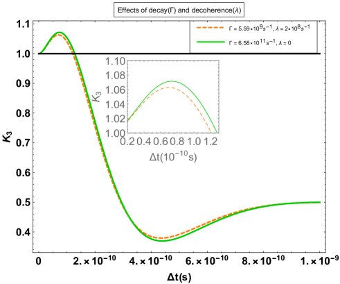
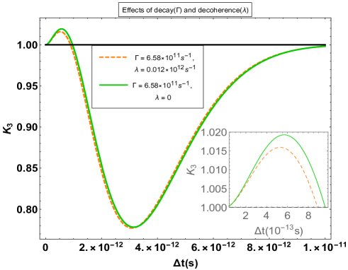
We see from FIG. 1, that there is a very clear violation of the upper bound limit of $K_{3}$ which goes beyond 1 specifically for almost all the values between $\Delta t=0$ and $2\times 10^{-10}s$ depicted on the plot. Particularly, when the value of $\Delta t$ is around or equal to $10^{-10}s$ maximum violation is attained for the case when both parameters are involved in the oscillation. Also, we see the behavior of curves corresponding to when both decay and decoherence persist in the system and when there is no decoherence is almost the same. However, for the case when there is no decoherence it can be well observed that, when the interval of $\Delta t$ is $10^{-10}s$ the maximal violation obtained is greater as compared to the case when there were both decay and decoherence. This means the system of meson oscillation tends to exhibit maximal temporal correlation when its flavour eigen states are coherent than when it is not.

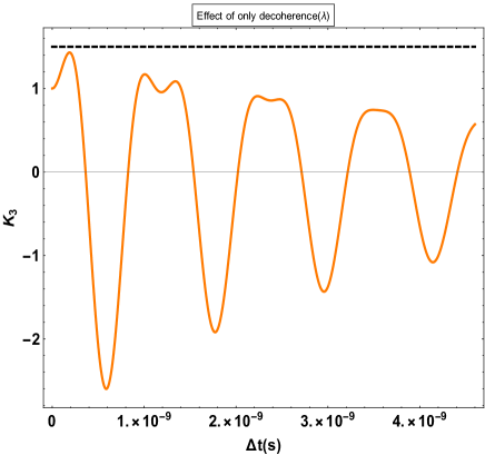
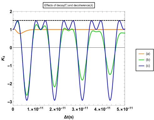
Suppose, now if we turn off both the decay and decoherence effects governing in these oscillations will lead to a different scenario. The expressions for probabilities and LGI function will change as:

  • Removing decay effects:

    $\displaystyle P_{\bar{K}^{0}\bar{K}^{0}}=\frac{1}{2}\left[1+e^{-\lambda t}\cos{(\Delta mt)}\right]$ (52)
    K3=14PK¯0K0(Δt)+8PK¯0K0(Δt)PK¯0K¯0(Δt)subscript𝐾314subscript𝑃superscript¯𝐾0superscript𝐾0Δ𝑡8subscript𝑃superscript¯𝐾0superscript𝐾0Δ𝑡subscript𝑃superscript¯𝐾0superscript¯𝐾0Δ𝑡\displaystyle K_{3}=1-4P_{\bar{K}^{0}K^{0}}(\Delta t)+8P_{\bar{K}^{0}K^{0}}(\Delta t)P_{\bar{K}^{0}\bar{K}^{0}}(\Delta t)
    $\displaystyle+\left|{{\frac{p}{q}}}\right|^{2}\left(e^{-2\lambda\Delta t}-1\right)$ (53)
Refer to caption
Figure 2: Plot for $K_{3}$ vs $\Delta t$ when decay effect is completely neglected and decoherence is taken into account. The horizontal shaded line denotes the maximum quantum mechanical violation for $K_{3}$.
  • Removing decay and decoherence effects:

    $\displaystyle P_{\bar{K}^{0}\bar{K}^{0}}=\frac{1}{2}\left[1+\cos{(\Delta mt)}\right]$ (54)
    $\displaystyle K_{3}=1-4P_{\bar{K}^{0}K^{0}}(\Delta t)+8P_{\bar{K}^{0}K^{0}}(\Delta t)P_{\bar{K}^{0}\bar{K}^{0}}(\Delta t)$ (55)
Refer to caption
Figure 3: Plot for $K_{3}$ vs $\Delta t$ when both decay and decoherence effects are completely neglected.The horizontal shaded line denotes the maximum quantum mechanical violation for $K_{3}$.

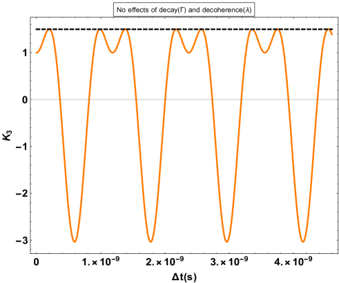
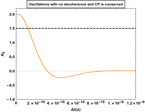
From FIG. 2 & FIG. 3, intuitively we get the violations again, here we can see the oscillatory behavior of probabilities which is still preserved in both the cases, this feature exists because the decay effect is completely neglected. However, in the latter case, the decoherence effect is too neglected making it look like a very ideal oscillatory system. Thus, again the meson system is completely coherent, and we see the maximal violation at successive intervals of $\Delta t$ where it attains the upper saturation bound of $1.5$. In the other case, we see the behavior of the curve is attenuating where the strength of amplitude decreases successively with the same $\Delta t$ interval. This happens because the temporal frequency or mixing parameter of mesons $\Delta m$ is kept fixed. The upper limit maximum violation in the FIG. 2 is achieved around when the value of $\Delta t=0.2\times 10^{-9}s$ which is just below $K_{3}=1.5$ and the violation gradually decreases at successive intervals of $\Delta t$. In contrast, FIG. 3 depicts the maximum violation is always repeated after every successive $\Delta t$. This particular sort of behavior if persists in mesons then we can exploit it in various interferometry examinations leading to the test of noninvasive measurability Joarder . Now, we can properly make an illustrative comparison in the following figure which will sum up all the different cases in a single picture.

Refer to caption
Figure 4: Plot for $K_{3}$ vs $\Delta t$ for three different cases, i.e., (a). oscillations without decay and decoherence given by red ($\Gamma\neq 0$ & $\lambda\neq 0$), (b). oscillations without decay and with decoherence given by green ($\Gamma=0$ & $\lambda\neq 0$) and (c). oscillations with decay and decoherence given by blue ($\Gamma=0$ & $\lambda=0$). The horizontal shaded line denotes the maximum quantum mechanical violation for $K_{3}$.

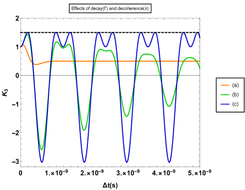
Now, from FIG. 4, it is indicative that how the practical situation of oscillation i.e., when both decay and decoherence are involved is very different from the response of other scenarios. We see maximum violation is achieved only for specific interval $\Delta t$, as we saw in FIG. 1, otherwise, it always saturates to lower limit of LGI $K_{3}=0.5$ for intervals $\Delta t\geq 10^{-9}s$. Also again from FIG 1, we can verify that the upper quantum bound, $K_{3}=1.5$ never attained in this case which is far from the upper quantum saturation mark. The important outtake which we can derive from FIG. 1 & 4 is whenever we have a system that is completely devoid of decay effects $\Gamma=0$ (or practically we can say observing a system at very negligible time interval which is just comparable to their lifetime), then we find that system to always attaining the maximal violation of $K_{3}=1.5$ or attains the maximum value just below it. Also, when we completely cut down the interaction of environment ($\lambda=0$) then it turns out to act as a very coherent oscillation system. This allows one to infer that if there is no quantum decoherence in flavor oscillations of meson system then it will always saturate the temporal Tsirelson bound cirel'son for at least a specific temporally separated $\Delta t$ and correlated flavor states. This means particularly these temporally correlated states will exhibit maximal entanglement in time compared to any other cases. This is just like the maximal violation of Bell inequality for a given bipartite two-qubit state Maximal_violation .

So far, what we have observed is all about the $K$-mesons, now we can turn to $B_{d}$-mesons. Here too, we are going to have the same behavior for variation of $K_{3}$. But still, there can be some subtleties to watch out for since both mesons have different quark contents, thereby, making them have different decay modes, mixing parameters, etc.

Refer to caption
Figure 5: Plot for $K_{3}$ vs $\Delta t$. Again, the red shaded curve and green bold curve corresponds to $\Gamma\neq 0$; $\lambda\neq 0$ and $\Gamma\neq 0$; $\lambda=0$ respectively. The horizontal black line denotes the maximum value of $K_{3}$ allowed by LGI. The CP violating parameter is taken to be $\left|\frac{q}{p}\right|=1.010$ DAmbrosio:2006hes . Other values are taken as $\Delta\Gamma=0$ and $\Delta m=0.5064\times 10^{12}s^{-1}$ ParticleDataGroup:2016lqr
Refer to caption
Figure 6: Plot for $K_{3}$ vs $\Delta t$ for three different cases: (a). $\Gamma\neq 0$ & $\lambda\neq 0$, (b). $\Gamma=0$ & $\lambda\neq 0$ and (c). $\Gamma=0$ & $\lambda=0$. The horizontal shaded line denotes the maximum quantum mechanical violation for $K_{3}$.

Now, FIG. 5 and 6 gives very similar responses to what we found in $K$-mesons. Here also, we see whenever there is complete coherence in the oscillations or practically if we study the system for a very small time intervals compared to the lifetimes, then we find the system maximally violates the LGI or saturates the Tsirelson bound (upper quantum bound; $K_{3}=1.5$). However, in $B_{d}$-mesons for the case when both decay and decoherence are involved, there is little different behavior unlike in $K$-mesons. The upper limit of $K_{3}$ value as predicted by LGI (or also $K_{3}>1$) for K-mesons is only reached for very short instant and otherwise it takes the constant value of $K_{3}=0.5$ for all the higher intervals $\Delta t$. But in $B_{d}$-mesons, except for some small interval, its value always stays at 1.

Suppose, if we digress back to the study of meson oscillation in the context of CP conservation in the section [I.2], we can refer to their probabilities and construct the correlation and LGI function accordingly. Again invoking the equal time interval measurement assumption on the $K$-meson oscillation when initially it was started with $\ket{K^{0}}$ state, then we would yield the following results from the definitions as stated in equations (4) and (I.1.1);

$\displaystyle C_{12}(\Delta t)=2(P_{K^{0}K^{0}}(\Delta t)-P_{K^{0}\bar{K^{0}}}(\Delta t))$ (56)

&

$\displaystyle K_{3}=2C_{12}(\Delta t)-C_{12}(2\Delta t)$ (57)

where $P_{K^{0}K^{0}}$ and $P_{K^{0}\bar{K^{0}}}$ are the expressions of probabilities as given in equations (I.2) and (I.2).

Refer to caption
Figure 7: Plot for $K_{3}$ vs $\Delta t$ for CP eigenstates of $K$-mesons. The horizontal shaded line denotes the maximum quantum mechanical violation for $K_{3}$.

In the context of oscillations of CP eigenstates of $K$-mesons has even more weird results to show. The value of $K_{3}$ for some intervals of $\Delta t$, crosses over the maximum quantum mechanical correlated value of 1.5. We can see for some initial small interval of $\Delta t$, it takes the value of $K_{3}=2$, also much like the non-CP states, as we saw earlier, the behavior of $K_{3}$ over various successive intervals of $\Delta t$ remains pretty much the same, except it takes different values for $K_{3}$. From the perspective of LGI, the value of K crossing over the mark of temporal Tsirelson bound has something more to hint that the measurement leads to greater wave function collapse than the projective measurements we saw earlier. Other experiments have already shown these sort of enhanced violations in LGI, like at $PT$ symmetry breaking point Karthik:2019wbp ; Wang . May be this could be just signifying that the natural systems of mesons are never CP conserved so this could state that they are unphysical phenomena that are just limited to theoretical analysis in the context of LGI. A similar result will also follow for $B$-meson oscillation system.

III Conclusion

The study of LGI has revealed productive outcomes in deciphering the actual behavior of physical systems. Implementing LGI in our understanding of mesons oscillation system has equally been very useful in knowing various intrinsic aspects governing the role of oscillations. We found how these oscillation systems can be treated as an exemplary open quantum system where we saw how the interaction of the environment with the system plays out the role of decoherence Shafaq:2021lju . LGI further helped us know how much maximum correlation exists between the oscillating states in account of both decay and decoherence. Decoherence generally suppresses the LGI violation compared to the situation when oscillations take place coherently. Temporal Tsirelson bound is nearly or fully achieved only whenever decay effects are neglected, i.e., taking measurements at small intervals comparable to their mean proper lifetime. The persisting oscillation behavior obtained in few cases can be put into use to carry out loophole free interferometric test at the experimental level as has been performed out in ref. Joarder and the references therein using heralded single photons. Finally, we also produced the naive treatment of meson oscillation in terms of CP eigenstates which showed weird results of LGI violation, where the violations were over enhanced (or crossing the mark of Tsirelson bound).This could signify some hidden phenomenon playing out, or may be it could be stating a mere unphysical phenomenon where CP is supposed to be conserved in the weak interaction and mesons decay via the weak interaction. Thus, LGI helps us to unfold various aspects behind the $K$- and $B-$ meson physics at its intricate features.

IV Acknowledgement

One of the author, KS wants to thank Prof. Prasanta K Panigrahi for the hospitality and useful discussions during her research visit on April 2022, at IISER, Kolkata. KS is also thankful to the Ministry of Education, Govt of India for financial support. Also, Aryabrat Mahapatra, a second year student of MSc from IIT Bhubaneswar would like to acknowledge Dr. Sudhanwa Patra for the fruitful discussion during the internship period of June-July, 2022.

Appendix A Evolution of density matrix in time using Kraus representation

The evolution of density matrix for the oscillations of $K^{0}-\bar{K^{0}}$ when the initial state is $\ket{K^{0}}$;

$\displaystyle\rho_{K^{0}}(t)$ $\displaystyle=$ $\displaystyle\sum_{i}\mathcal{K}_{i}\rho_{K^{0}}(0)\mathcal{K}_{i}^{\dagger}$
$\displaystyle=$ $\displaystyle\mathcal{K}_{0}\rho_{K^{0}}(0)\mathcal{K}_{0}^{\dagger}+\mathcal{K}_{1}\rho_{K^{0}}(0)\mathcal{K}_{1}^{\dagger}+...+\mathcal{K}_{5}\rho_{K^{0}}(0)\mathcal{K}_{5}^{\dagger}$

where $\rho_{K^{0}}(0)=\ket{K^{0}}\bra{K^{0}}$,    i.e.,  $\rho_{K^{0}}(0)=\begin{pmatrix}1\\ 0\\ 0\end{pmatrix}\begin{pmatrix}1&0&0\end{pmatrix}=\begin{pmatrix}1&0&0\\ 0&0&0\\ 0&0&0\end{pmatrix}.$ So,

$\displaystyle\mathcal{K}_{0}\rho_{K^{0}}(0)\mathcal{K}_{0}^{\dagger}$ $\displaystyle=$ $\displaystyle(\ket{0}\bra{0})(\ket{K^{0}}\bra{K^{0}})(\ket{0}\bra{0})^{\dagger}=0$
$\displaystyle\mathcal{K}_{1}\rho_{K^{0}}(0)\mathcal{K}_{1}^{\dagger}$ $\displaystyle=$ $\displaystyle(\mathcal{C}_{1+}(\ket{K^{0}}\bra{K^{0}}+\ket{\bar{K^{0}}}\bra{\bar{K^{0}}}+\mathcal{C}_{1-}(\frac{1+\epsilon}{1-\epsilon}\ket{K^{0}}\bra{\bar{K^{0}}}+\frac{1-\epsilon}{1+\epsilon}\ket{\bar{K^{0}}}\bra{K^{0}}))(\ket{K^{0}}\bra{K^{0}})$
$\displaystyle(\mathcal{C}_{1+}(\ket{K^{0}}\bra{K^{0}}+\ket{\bar{K^{0}}}\bra{\bar{K^{0}}}+\mathcal{C}_{1-}(\frac{1+\epsilon}{1-\epsilon}\ket{K^{0}}\bra{\bar{K^{0}}}+\frac{1-\epsilon}{1+\epsilon}\ket{\bar{K^{0}}}\bra{K^{0}}))^{\dagger}$
$\displaystyle=$ $\displaystyle|\mathcal{C}_{1+}|^{2}\ket{K^{0}}\bra{K^{0}}+\mathcal{C}_{1+}\mathcal{C}_{1-}^{*}(\frac{1-\epsilon}{1+\epsilon})^{*}\ket{K^{0}}\bra{\bar{K^{0}}}+\mathcal{C}_{1+}^{*}\mathcal{C}_{1-}(\frac{1-\epsilon}{1+\epsilon})\ket{\bar{K^{0}}}\bra{K^{0}}+|\mathcal{C}_{1-}|^{2}|\frac{1-\epsilon}{1+\epsilon}|^{2}\ket{\bar{K^{0}}}\bra{\bar{K^{0}}}$
$\displaystyle=$ $\displaystyle\begin{pmatrix}|\mathcal{C}_{1+}|^{2}&\mathcal{C}_{1+}\mathcal{C}_{1-}^{*}(\frac{1-\epsilon}{1+\epsilon})^{*}&0\\ \mathcal{C}_{1+}^{*}\mathcal{C}_{1-}(\frac{1-\epsilon}{1+\epsilon})&|\mathcal{C}_{1-}|^{2}|\frac{1-\epsilon}{1+\epsilon}|^{2}&0\\ 0&0&0\\ \end{pmatrix}$
$\displaystyle\mathcal{K}_{2}\rho_{K^{0}}(0)\mathcal{K}_{2}^{\dagger}$ $\displaystyle=$ $\displaystyle(\mathcal{C}_{2}(\frac{1}{1+\epsilon}\ket{0}\bra{K^{0}}+\frac{1}{1-\epsilon}\ket{0}\bra{\bar{K^{0}}}))(\ket{K^{0}}\bra{K^{0}})(\mathcal{C}_{2}(\frac{1}{1+\epsilon}\ket{0}\bra{K^{0}}+\frac{1}{1-\epsilon}\ket{0}\bra{\bar{K^{0}}}))^{\dagger}$
$\displaystyle=$ $\displaystyle|\mathcal{C}_{2}|^{2}\left|\frac{1}{1+\epsilon}\right|^{2}\ket{0}\bra{0}$
$\displaystyle=$ $\displaystyle\begin{pmatrix}0&0&0\\ 0&0&0\\ 0&0&|\mathcal{C}_{2}|^{2}\left|\frac{1}{1+\epsilon}\right|^{2}\\ \end{pmatrix}$
$\displaystyle\mathcal{K}_{3}\rho_{K^{0}}(0)\mathcal{K}_{3}^{\dagger}$ $\displaystyle=$ $\displaystyle(\mathcal{C}_{3+}\frac{1}{1+\epsilon}\ket{0}\bra{K^{0}}+\mathcal{C}_{3-}\frac{1}{1-\epsilon}\ket{0}\bra{\bar{K^{0}}})(\ket{K^{0}}\bra{K^{0}})(\mathcal{C}_{3+}\frac{1}{1+\epsilon}\ket{0}\bra{K^{0}}+\mathcal{C}_{3-}\frac{1}{1-\epsilon}\ket{0}\bra{\bar{K^{0}}})^{\dagger}$
$\displaystyle=$ $\displaystyle|\mathcal{C}_{3+}|^{2}\left|\frac{1}{1+\epsilon}\right|^{2}\ket{0}\bra{0}$
$\displaystyle=$ $\displaystyle\begin{pmatrix}0&0&0\\ 0&0&0\\ 0&0&|\mathcal{C}_{3+}|^{2}\left|\frac{1}{1+\epsilon}\right|^{2}\\ \end{pmatrix}$
$\displaystyle\mathcal{K}_{4}\rho_{K^{0}}(0)\mathcal{K}_{4}^{\dagger}$ $\displaystyle=$ $\displaystyle(\mathcal{C}_{4}(\ket{K^{0}}\bra{K^{0}}+\ket{\bar{K^{0}}}\bra{\bar{K^{0}}}+\frac{1+\epsilon}{1-\epsilon}\ket{K^{0}}\bra{\bar{K^{0}}}+\frac{1-\epsilon}{1+\epsilon}\ket{\bar{K^{0}}}\bra{K^{0}}))(\ket{K^{0}}\bra{K^{0}})$
$\displaystyle(\mathcal{C}_{4}(\ket{K^{0}}\bra{K^{0}}+\ket{\bar{K^{0}}}\bra{\bar{K^{0}}}+\frac{1+\epsilon}{1-\epsilon}\ket{K^{0}}\bra{\bar{K^{0}}}+\frac{1-\epsilon}{1+\epsilon}\ket{\bar{K^{0}}}\bra{K^{0}}))^{\dagger}$
$\displaystyle=$ $\displaystyle|\mathcal{C}_{4}|^{2}\ket{K^{0}}\bra{K^{0}}+|\mathcal{C}_{4}|^{2}(\frac{1-\epsilon}{1+\epsilon})^{*}\ket{K^{0}}\bra{\bar{K^{0}}}+|\mathcal{C}_{4}|^{2}\left(\frac{1-\epsilon}{1+\epsilon}\right)^{*}\ket{\bar{K^{0}}}\bra{K^{0}}+|\mathcal{C}_{4}|^{2}\left|\frac{1-\epsilon}{1+\epsilon}\right|^{2}\ket{\bar{K^{0}}}\bra{\bar{K^{0}}}$
$\displaystyle=$ $\displaystyle\begin{pmatrix}|\mathcal{C}_{4}|^{2}&|\mathcal{C}_{4}|^{2}(\frac{1-\epsilon}{1+\epsilon})^{*}&0\\ |\mathcal{C}_{4}|^{2}(\frac{1-\epsilon}{1+\epsilon})&|\mathcal{C}_{4}|^{2}\left|\frac{1-\epsilon}{1+\epsilon}\right|^{2}&0\\ 0&0&0\end{pmatrix}$
$\displaystyle\mathcal{K}_{5}\rho_{K^{0}}(0)\mathcal{K}_{5}^{\dagger}$ $\displaystyle=$ $\displaystyle(\mathcal{C}_{5}(\ket{K^{0}}\bra{K^{0}}+\ket{\bar{K^{0}}}\bra{\bar{K^{0}}}-\frac{1+\epsilon}{1-\epsilon}\ket{K^{0}}\bra{\bar{K^{0}}}-\frac{1-\epsilon}{1+\epsilon}\ket{\bar{K^{0}}}\bra{K^{0}}))(\ket{K^{0}}\bra{K^{0}})$
$\displaystyle(\mathcal{C}_{5}(\ket{K^{0}}\bra{K^{0}}+\ket{\bar{K^{0}}}\bra{\bar{K^{0}}}-\frac{1+\epsilon}{1-\epsilon}\ket{K^{0}}\bra{\bar{K^{0}}}-\frac{1-\epsilon}{1+\epsilon}\ket{\bar{K^{0}}}\bra{K^{0}}))^{\dagger}$
$\displaystyle=$ $\displaystyle|\mathcal{C}_{5}|^{2}\ket{K^{0}}\bra{K^{0}}-|\mathcal{C}_{5}|^{2}(\frac{1-\epsilon}{1+\epsilon})^{*}\ket{K^{0}}\bra{\bar{K^{0}}}-|\mathcal{C}_{5}|^{2}\left(\frac{1-\epsilon}{1+\epsilon}\right)\ket{\bar{K^{0}}}\bra{K^{0}}+|\mathcal{C}_{5}|^{2}\left|\frac{1-\epsilon}{1+\epsilon}\right|^{2}\ket{\bar{K^{0}}}\bra{\bar{K^{0}}}$
$\displaystyle=$ $\displaystyle\begin{pmatrix}|\mathcal{C}_{5}|^{2}&-|\mathcal{C}_{5}|^{2}(\frac{1-\epsilon}{1+\epsilon})^{*}&0\\ -|\mathcal{C}_{5}|^{2}(\frac{1-\epsilon}{1+\epsilon})&|\mathcal{C}_{5}|^{2}\left|\frac{1-\epsilon}{1+\epsilon}\right|^{2}&0\\ 0&0&0\end{pmatrix}$
$\displaystyle\therefore\rho_{K^{0}}(t)=\begin{pmatrix}|\mathcal{C}_{1+}|^{2}+|\mathcal{C}_{4}|^{2}+|\mathcal{C}_{5}|^{2}&(\frac{1-\epsilon}{1+\epsilon})^{*}(\mathcal{C}_{1+}\mathcal{C}_{1-}^{*}+|\mathcal{C}_{4}|^{2}-|\mathcal{C}_{5}|^{2})&0\\ (\frac{1-\epsilon}{1+\epsilon})(\mathcal{C}_{1+}\mathcal{C}_{1-}^{*}+|\mathcal{C}_{4}|^{2}-|\mathcal{C}_{5}|^{2})&\left|\frac{1-\epsilon}{1+\epsilon}\right|^{2}(|\mathcal{C}_{1-}|^{2}+|\mathcal{C}_{4}|^{2}+|\mathcal{C}_{5}|^{2})&0\\ 0&0&\left|\frac{1}{1+\epsilon}\right|^{2}(|\mathcal{C}_{2}|^{2}+|\mathcal{C}_{3+}|^{2})\end{pmatrix}$

Now, using the coefficient values from equations (I.3), we will get the desired matrix as given in equation (I.3).

Appendix B Computing the two-time correlation function in terms of Kraus operators

The general expression for probabilities as obtained earlier is:

$\displaystyle p(^{a}t_{i})q(^{b}t_{j}|^{a}t_{i})=Tr\left\{\Pi^{b}\sum_{\nu,\mu}\mathcal{K}_{\nu}(t_{j}-t_{i})\Pi^{a}\sum_{\mu}\mathcal{K}_{\mu}(t_{i})\rho(0)\mathcal{K}_{\mu}^{\dagger}(t_{i})\Pi^{a}\mathcal{K}_{\nu}^{\dagger}(t_{j}-t_{i})\right\}$

The projector operators for the dichotomic observable which are involved here also satisfies a relation as $\Pi^{+}+\Pi^{-}=I$ The two-time correlation function is expanded in these probabilities as Castillo :

$\displaystyle C(t_{i},t_{j})=p(^{+}t_{i})q(^{+}t_{j}|^{+}t_{i})-p(^{+}t_{i})q(^{-}t_{j}|^{+}t_{i})-p(^{-}t_{i})q(^{+}t_{j}|^{-}t_{i})+p(^{-}t_{i})q(^{-}t_{j}|^{-}t_{i})$

where,

$\displaystyle p(^{+}t_{i})q(^{+}t_{j}|^{+}t_{i})$ $\displaystyle=$ $\displaystyle Tr\left\{\Pi^{+}\sum_{\nu,\mu}\mathcal{K}_{\nu}(t_{j}-t_{i})\Pi^{+}\mathcal{K}_{\mu}(t_{i})\rho(0)\mathcal{K}_{\mu}^{\dagger}(t_{i})\Pi^{+}\mathcal{K}_{\nu}^{\dagger}(t_{j}-t_{i})\right\}$
$\displaystyle p(^{-}t_{i})q(^{-}t_{j}|^{-}t_{i})$ $\displaystyle=$ $\displaystyle Tr\left\{\Pi^{-}\sum_{\nu,\mu}\mathcal{K}_{\nu}(t_{j}-t_{i})\Pi^{-}\mathcal{K}_{\mu}(t_{i})\rho(0)\mathcal{K}_{\mu}^{\dagger}(t_{i})\Pi^{-}\mathcal{K}_{\nu}^{\dagger}(t_{j}-t_{i})\right\}$
$\displaystyle=$ $\displaystyle Tr\left\{(I-\Pi^{+})\sum_{\nu,\mu}\mathcal{K}_{\nu}(t_{j}-t_{i})(I-\Pi^{+})\mathcal{K}_{\mu}(t_{i})\rho(0)\mathcal{K}_{\mu}^{\dagger}(t_{i})(I-\Pi^{+})\mathcal{K}_{\nu}^{\dagger}(t_{j}-t_{i})\right\}$
$\displaystyle=$ $\displaystyle Tr\left\{\sum_{\nu,\mu}\mathcal{K}_{\nu}(t_{j}-t_{i})(I-\Pi^{+})\mathcal{K}_{\mu}(t_{i})\rho(0)\mathcal{K}_{\mu}^{\dagger}(t_{i})(I-\Pi^{+})\mathcal{K}_{\nu}^{\dagger}(t_{j}-t_{i})\right\}$
$\displaystyle-Tr\left\{\Pi^{+}\sum_{\nu,\mu}\mathcal{K}_{\nu}(t_{j}-t_{i})(I-\Pi^{+})\mathcal{K}_{\mu}(t_{i})\rho(0)\mathcal{K}_{\mu}^{\dagger}(t_{i})(I-\Pi^{+})\mathcal{K}_{\nu}^{\dagger}(t_{j}-t_{i})\right\}$
$\displaystyle=$

$Tr\left\{\sum_{\nu,\mu}\mathcal{K}_{\nu}(t_{j}-t_{i})\mathcal{K}_{\mu}(t_{i})\rho(0)\mathcal{K}_{\mu}^{\dagger}(t_{i})\mathcal{K}_{\nu}^{\dagger}(t_{j}-t_{i})\right\}-Tr\left\{\sum_{\nu,\mu}\mathcal{K}_{\nu}(t_{j}-t_{i})\mathcal{K}_{\mu}(t_{i})\rho(0)\mathcal{K}_{\mu}^{\dagger}(t_{i})\Pi^{+}\mathcal{K}_{\nu}^{\dagger}(t_{j}-t_{i})\right\}$

$-Tr\left\{\sum_{\nu,\mu}\mathcal{K}_{\nu}(t_{j}-t_{i})\Pi^{+}\mathcal{K}_{\mu}(t_{i})\rho(0)\mathcal{K}_{\mu}^{\dagger}(t_{i})\mathcal{K}_{\nu}^{\dagger}(t_{j}-t_{i})\right\}+Tr\left\{\sum_{\nu,\mu}\mathcal{K}_{\nu}(t_{j}-t_{i})\Pi^{+}\mathcal{K}_{\mu}(t_{i})\rho(0)\mathcal{K}_{\mu}^{\dagger}(t_{i})\Pi^{+}\mathcal{K}_{\nu}^{\dagger}(t_{j}-t_{i})\right\}$

$-Tr\left\{\Pi^{+}\sum_{\nu,\mu}\mathcal{K}_{\nu}(t_{j}-t_{i})\mathcal{K}_{\mu}(t_{i})\rho(0)\mathcal{K}_{\mu}^{\dagger}(t_{i})\mathcal{K}_{\nu}^{\dagger}(t_{j}-t_{i})\right\}+Tr\left\{\Pi^{+}\sum_{\nu,\mu}\mathcal{K}_{\nu}(t_{j}-t_{i})\mathcal{K}_{\mu}(t_{i})\rho(0)\mathcal{K}_{\mu}^{\dagger}(t_{i})\Pi^{+}\mathcal{K}_{\nu}^{\dagger}(t_{j}-t_{i})\right\}$

$+Tr\left\{\Pi^{+}\sum_{\nu,\mu}\mathcal{K}_{\nu}(t_{j}-t_{i})\Pi^{+}\mathcal{K}_{\mu}(t_{i})\rho(0)\mathcal{K}_{\mu}^{\dagger}(t_{i})\mathcal{K}_{\nu}^{\dagger}(t_{j}-t_{i})\right\}-Tr\left\{\Pi^{+}\sum_{\nu,\mu}\mathcal{K}_{\nu}(t_{j}-t_{i})\Pi^{+}\mathcal{K}_{\mu}(t_{i})\rho(0)\mathcal{K}_{\mu}^{\dagger}(t_{i})\Pi^{+}\mathcal{K}_{\nu}^{\dagger}(t_{j}-t_{i})\right\}$

$\displaystyle p(^{-}t_{i})q(^{+}t_{j}|^{-}t_{i})$ $\displaystyle=$ $\displaystyle Tr\left\{\Pi^{+}\sum_{\nu,\mu}\mathcal{K}_{\nu}(t_{j}-t_{i})\Pi^{-}\mathcal{K}_{\mu}(t_{i})\rho(0)\mathcal{K}_{\mu}^{\dagger}(t_{i})\Pi^{-}\mathcal{K}_{\nu}^{\dagger}(t_{j}-t_{i})\right\}$
$\displaystyle=$ $\displaystyle Tr\left\{\Pi^{+}\sum_{\nu,\mu}\mathcal{K}_{\nu}(t_{j}-t_{i})(I-\Pi^{+})\mathcal{K}_{\mu}(t_{i})\rho(0)\mathcal{K}_{\mu}^{\dagger}(t_{i})(I-\Pi^{+})\mathcal{K}_{\nu}^{\dagger}(t_{j}-t_{i})\right\}$
$\displaystyle=$

$Tr\left\{\Pi^{+}\sum_{\nu,\mu}\mathcal{K}_{\nu}(t_{j}-t_{i})\mathcal{K}_{\mu}(t_{i})\rho(0)\mathcal{K}_{\mu}^{\dagger}(t_{i})\mathcal{K}_{\nu}^{\dagger}(t_{j}-t_{i})\right\}-Tr\left\{\Pi^{+}\sum_{\nu,\mu}\mathcal{K}_{\nu}(t_{j}-t_{i})\mathcal{K}_{\mu}(t_{i})\rho(0)\mathcal{K}_{\mu}^{\dagger}(t_{i})\Pi^{+}\mathcal{K}_{\nu}^{\dagger}(t_{j}-t_{i})\right\}$

$-Tr\left\{\Pi^{+}\sum_{\nu,\mu}\mathcal{K}_{\nu}(t_{j}-t_{i})\Pi^{+}\mathcal{K}_{\mu}(t_{i})\rho(0)\mathcal{K}_{\mu}^{\dagger}(t_{i})\mathcal{K}_{\nu}^{\dagger}(t_{j}-t_{i})\right\}+Tr\left\{\Pi^{+}\sum_{\nu,\mu}\mathcal{K}_{\nu}(t_{j}-t_{i})\Pi^{+}\mathcal{K}_{\mu}(t_{i})\rho(0)\mathcal{K}_{\mu}^{\dagger}(t_{i})\Pi^{+}\mathcal{K}_{\nu}^{\dagger}(t_{j}-t_{i})\right\}$

$\displaystyle p(^{+}t_{i})q(^{-}t_{j}|^{+}t_{i})$ $\displaystyle=$ $\displaystyle Tr\left\{\Pi^{-}\sum_{\nu,\mu}\mathcal{K}_{\nu}(t_{j}-t_{i})\Pi^{+}\mathcal{K}_{\mu}(t_{i})\rho(0)\mathcal{K}_{\mu}^{\dagger}(t_{i})\Pi^{+}\mathcal{K}_{\nu}^{\dagger}(t_{j}-t_{i})\right\}$
$\displaystyle=$ $\displaystyle Tr\left\{(I-\Pi^{+})\sum_{\nu,\mu}\mathcal{K}_{\nu}(t_{j}-t_{i})\Pi^{+}\mathcal{K}_{\mu}(t_{i})\rho(0)\mathcal{K}_{\mu}^{\dagger}(t_{i})\Pi^{+}\mathcal{K}_{\nu}^{\dagger}(t_{j}-t_{i})\right\}$
$\displaystyle=$

$Tr\left\{\sum_{\nu,\mu}\mathcal{K}_{\nu}(t_{j}-t_{i})\mathcal{K}_{\mu}(t_{i})\rho(0)\mathcal{K}_{\mu}^{\dagger}(t_{i})\mathcal{K}_{\nu}^{\dagger}(t_{j}-t_{i})\right\}-Tr\left\{\Pi^{+}\sum_{\nu,\mu}\mathcal{K}_{\nu}(t_{j}-t_{i})\Pi^{+}\mathcal{K}_{\mu}(t_{i})\rho(0)\mathcal{K}_{\mu}^{\dagger}(t_{i})\Pi^{+}\mathcal{K}_{\nu}^{\dagger}(t_{j}-t_{i})\right\}$

Thus, correlation function will now become:

$\displaystyle C(t_{i},t_{j})$ $\displaystyle=$

$1-2Tr\left\{\Pi^{+}\sum_{\nu,\mu}\mathcal{K}_{\nu}(t_{j}-t_{i})\mathcal{K}_{\mu}(t_{i})\rho(0)\mathcal{K}_{\mu}^{\dagger}(t_{i})\mathcal{K}_{\nu}^{\dagger}(t_{j}-t_{i})\right\}-Tr\left\{\sum_{\nu,\mu}\mathcal{K}_{\nu}(t_{j}-t_{i})\Pi^{+}\mathcal{K}_{\mu}(t_{i})\rho(0)\mathcal{K}_{\mu}^{\dagger}(t_{i})\mathcal{K}_{\nu}^{\dagger}(t_{j}-t_{i})\right\}$

$-Tr\left\{\sum_{\nu,\mu}\mathcal{K}_{\nu}(t_{j}-t_{i})\mathcal{K}_{\mu}(t_{i})\rho(0)\mathcal{K}_{\mu}^{\dagger}(t_{i})\Pi^{+}\mathcal{K}_{\nu}^{\dagger}(t_{j}-t_{i})\right\}+2Tr\left\{\Pi^{+}\sum_{\nu,\mu}\mathcal{K}_{\nu}(t_{j}-t_{i})\Pi^{+}\mathcal{K}_{\mu}(t_{i})\rho(0)\mathcal{K}_{\mu}^{\dagger}(t_{i})\mathcal{K}_{\nu}^{\dagger}(t_{j}-t_{i})\right\}$

$+Tr\left\{\Pi^{+}\sum_{\nu,\mu}\mathcal{K}_{\nu}(t_{j}-t_{i})\mathcal{K}_{\mu}(t_{i})\rho(0)\mathcal{K}_{\mu}^{\dagger}(t_{i})\Pi^{+}\mathcal{K}_{\nu}^{\dagger}(t_{j}-t_{i})\right\}$

The second term gives the probability of getting $+1$ when $\rho(0)$ is evolved till $t_{j}$ and third and fourth terms gives the probability of getting $+1$ when $\rho(0)$ is evolved till $t_{i}$,i.e. as following:

$\displaystyle p(^{+}t_{i})$ $\displaystyle=$ $\displaystyle Tr\left\{\sum_{\mu}\Pi^{+}\mathcal{K}_{\mu}(t_{i})\rho(0)\mathcal{K}_{\mu}^{\dagger}(t_{i})\right\}$
$\displaystyle=$ $\displaystyle Tr\left\{\sum_{\nu,\mu}\mathcal{K}_{\nu}(t_{j}-t_{i})\left[\Pi^{+}\mathcal{K}_{\mu}(t_{i})\rho(0)\mathcal{K}_{\mu}^{\dagger}(t_{i})\right]\mathcal{K}_{\nu}^{\dagger}(t_{j}-t_{i})\right\}$

The last two terms can be further rewritten as $2g(t_{i},t_{j})$ and its hermitian conjugate, where,

$\displaystyle g(t_{i},t_{j})=Tr\left\{\rho(0)\sum_{\nu,\mu}\mathcal{K}^{\dagger}_{\mu}(t_{i})\mathcal{K}^{\dagger}_{\nu}(t_{j}-t_{i})\Pi^{+}\mathcal{K}_{\nu}(t_{j}-t_{i})\mathcal{K}_{\mu}(t_{i})\right\}$

or

$\displaystyle g(t_{i},t_{j})$ $\displaystyle=$ $\displaystyle Tr\left\{\sum_{\nu,\mu}\Pi^{+}\mathcal{K}_{\nu}(t_{j}-t_{i})\Pi^{+}\mathcal{K}_{\mu}(t_{i})\rho(0){K}^{\dagger}_{\mu}(t_{i})\mathcal{K}^{\dagger}_{\nu}(t_{j}-t_{i})\right\}$
$\displaystyle=$ $\displaystyle Tr\left\{\Pi^{+}\sum_{\nu}\mathcal{K}_{\nu}(t_{j}-t_{i})\rho(t_{i})\mathcal{K}^{\dagger}_{\nu}(t_{j}-t_{i})\right\}$

Hence, two-time correlation can be written as in equation (45), i.e.;

$\displaystyle C(t_{i},t_{j})=1-2p(^{+}t_{i})-2p(^{+}t_{j})+4Re[g(t_{i},t_{j})]$

References

  • (1) A. Einstein, B. Podolsky, and N. Rosen Phys. Rev. 47, 777 – Published 15 May 1935
  • (2) Griffith, D., Introduction to Quantum Mechanics 2014. Essex: Pearson.
  • (3) Leggett, A.J. and Garg, A., 1985. Quantum mechanics versus macroscopic realism: Is the flux there when nobody looks?. Physical Review Letters, 54(9), p.857.
  • (4) Breuer, H.P. and Petruccione, F., 2002. The theory of open quantum systems. Oxford University Press on Demand.
  • (5) Banerjee, S., Alok, A.K. and MacKenzie, R., 2016. Quantum correlations in B and K meson systems. The European Physical Journal Plus, 131(5), pp.1-8.
  • (6) S. Banerjee, A. K. Alok and R. MacKenzie, Eur. Phys. J. Plus 131, no.5, 129 (2016) doi:10.1140/epjp/i2016-16129-0 [arXiv:1409.1034 [hep-ph]].
  • (7) J. Naikoo, S. Kumari, S. Banerjee and A. K. Pan
  • (8) J. Naikoo, A. K. Alok and S. Banerjee, Phys. Rev. D 97, no.5, 053008 (2018) doi:10.1103/PhysRevD.97.053008 [arXiv:1802.04265 [hep-ph]].
  • (9) Budroni, C. and Emary, C., 2014. Temporal quantum correlations and Leggett-Garg inequalities in multilevel systems. Physical review letters, 113(5), p.050401.
  • (10) J. Naikoo, A. Kumar Alok, S. Banerjee and S. Uma Sankar, Phys. Rev. D 99, no.9, 095001 (2019) doi:10.1103/PhysRevD.99.095001 [arXiv:1901.10859 [hep-ph]].
  • (11) J. Naikoo, A. K. Alok, S. Banerjee, S. Uma Sankar, G. Guarnieri, C. Schultze and B. C. Hiesmayr, Nucl. Phys. B 951, 114872 (2020) doi:10.1016/j.nuclphysb.2019.114872 [arXiv:1710.05562 [hep-ph]].
  • (12) Dixit, K., Naikoo, J., Banerjee, S. and Alok, A.K., 2019. Study of coherence and mixedness in meson and neutrino systems. The European Physical Journal C, 79(2), pp.1-7.
  • (13) Gangopadhyay, D., Home, D. and Roy, A.S., 2013. Probing the Leggett-Garg inequality for oscillating neutral kaons and neutrinos. Physical Review A, 88(2), p.022115.
  • (14) Saha, D., Mal, S., Panigrahi, P.K. and Home, D., 2015. Wigner’s form of the Leggett-Garg inequality, the no-signaling-in-time condition, and unsharp measurements. Physical Review A, 91(3), p.032117.
  • (15) S. Shafaq, T. Kushwaha and P. Mehta, [arXiv:2112.12726 [hep-ph]].
  • (16) Joarder, K., Saha, D., Home, D. and Sinha, U., 2022. Loophole-free interferometric test of macrorealism using heralded single photons. PRX Quantum, 3(1), p.010307.
  • (17) Goggin, M.E., Almeida, M.P., Barbieri, M., Lanyon, B.P., O’brien, J.L., White, A.G. and Pryde, G.J., 2011. Violation of the Leggett–Garg inequality with weak measurements of photons. Proceedings of the National Academy of Sciences, 108(4), pp.1256-1261.
  • (18) Katiyar, H., Brodutch, A., Lu, D. and Laflamme, R., 2017. Experimental violation of the Leggett–Garg inequality in a three-level system. New Journal of Physics, 19(2), p.023033.
  • (19) Murskyj, M., 2015. Testing the Leggett-Garg inequality with solar neutrinos (Doctoral dissertation, Massachusetts Institute of Technology).
  • (20) Weron, A., Rajagopal, A.K. and Weron, K., 1985. Quantum theory of decaying systems from the canonical decomposition of dynamical semigroups. Physical Review A, 31(3), p.1736.
  • (21) Emary, C., Lambert, N. and Nori, F., 2013. Leggett–garg inequalities. Reports on Progress in Physics, 77(1), p.016001.
  • (22) R. Belusevic, Springer Tracts Mod. Phys. 153, 1-182 (1999) KEK-PREPRINT-97-264.
  • (23) T. Banks, L. Susskind and M. E. Peskin, Nucl. Phys. B 244, 125-134 (1984) doi:10.1016/0550-3213(84)90184-6
  • (24) Nielsen, M.A. and Chuang, I., 2002. Quantum computation and quantum information.
  • (25) G. Lindblad, Commun. Math. Phys. 48, 119 (1976).
  • (26) Kraus, K., Böhm, A., Dollard, J.D. and Wootters, W.H. eds., 1983. States, Effects, and Operations Fundamental Notions of Quantum Theory: Lectures in Mathematical Physics at the University of Texas at Austin. Berlin, Heidelberg: Springer Berlin Heidelberg.
  • (27) Caban, P., Rembieliński, J., Smoliński, K.A. and Walczak, Z., 2005. Unstable particles as open quantum systems. Physical Review A, 72(3), p.032106. , J. Phys. G 47, no.9, 095004 (2020) doi:10.1088/1361-6471/ab9f9b [arXiv:1906.05995 [hep-ph]].
  • (28) Sarkar, U., 2007. Particle and Astroparticle physics. CRC Press.
  • (29) Castillo, J.C., Rodríguez, F.J. and Quiroga, L., 2013. Enhanced violation of a Leggett-Garg inequality under nonequilibrium thermal conditions. Physical Review A, 88(2), p.022104.
  • (30) Paz, J.P. and Mahler, G., 1993. Proposed test for temporal Bell inequalities. Physical review letters, 71(20), p.3235.
  • (31) Kofler, J. and Brukner, Č., 2008. Conditions for quantum violation of macroscopic realism. Physical review letters, 101(9), p.090403.
  • (32) Huelga, S.F., Marshall, T.W. and Santos, E., 1996. Temporal Bell-type inequalities for two-level Rydberg atoms coupled to a high-Q resonator. Physical Review A, 54(3), p.1798.
  • (33) Wilde, M.M., McCracken, J.M. and Mizel, A., 2010. Could light harvesting complexes exhibit non-classical effects at room temperature?. Proceedings of the Royal Society A: Mathematical, Physical and Engineering Sciences, 466(2117), pp.1347-1363.
  • (34) Y. Amhis et al. [HFLAV], Eur. Phys. J. C 77, no.12, 895 (2017) doi:10.1140/epjc/s10052-017-5058-4 [arXiv:1612.07233 [hep-ex]].
  • (35) Wang, K., Emary, C., Zhan, X., Bian, Z., Li, J. and Xue, P., 2017. Beyond the temporal Tsirelson bound: an experimental test of Leggett-Garg inequalities in a three-level system. arXiv preprint arXiv:1701.02454.
  • (36) XIANG Yang 2010 Chin. Phys. Lett. 27 120301
  • (37) G. D’Ambrosio et al. [KLOE], JHEP 12, 011 (2006) doi:10.1088/1126-6708/2006/12/011 [arXiv:hep-ex/0610034 [hep-ex]].
  • (38) C. Patrignani et al. [Particle Data Group], Chin. Phys. C 40, no.10, 100001 (2016) doi:10.1088/1674-1137/40/10/100001
  • (39) H. S. Karthik, A. Shenoy Hejamadi and A. R. U. Devi, Phys. Rev. A 103, no.3, 032420 (2021) doi:10.1103/PhysRevA.103.032420 [arXiv:1907.02879 [quant-ph]].
  • (40) Wang, K., Emary, C., Zhan, X., Bian, Z., Li, J. and Xue, P., 2017. Enhanced violations of Leggett-Garg inequalities in an experimental three-level system. Optics express, 25(25), pp.31462-31470.